Marzo-2017-prueba

Consulta de ejemplares
Vol. 88. núm. 1 (2017)
Marzo


Taxonomía y Sistemática


A new species of the genus Monstrilla (Copepoda: Monstrilloida: Monstrillidae) from the Gulf of California, Mexico
Eduardo Suárez-Morales a, *, Karl E. Velázquez-Ornelas b
a El Colegio de la Frontera Sur, Avenida Centenario Km 5.5, 77014 Chetumal, Quintana Roo, Mexico
b Universidad Nacional Autónoma de México, Instituto de Ciencias del Mar y Limnología, Unidad Mazatlán, Joel Montes Camarena s/n, 82040 Mazatlán, Sinaloa, Mexico
*Corresponding author: esuarez@ecosur.mx (E. Suárez-Morales)
Received: 23 September 2023; accepted: 24 June 2024
http://zoobank.org/urn:lsid:zoobank.org:pub:55476587-382E-4014-9EB2-F111CFF305DC
Abstract
Based on deep-water (700-750 m) biological samples obtained from the southern Gulf of California, Pacific coast of Mexico, a new species of the monstrilloid copepod genus Monstrilla Dana, 1849 is described based on a single subadult female collected close to the bottom with an epibenthic sledge. Monstrilla hendrickxi sp. n. is distinguished by a unique combination of characters including: 1) no trace of eyes; 2) strong, thick antennules with segments 2-4 partly fused; 3) strongly developed apical elements on antennular segment 5 and spinous processes on segments 2-5; and 4) bilobed fifth legs with 2 apical setae on the exopodal lobe and a digitiform, unarmed endopodal lobe. The new species exhibits some affinity with surface-dwelling species of Monstrilla that have 2 setae on the exopodal lobes of the fifth legs. This is the fifth record of a species of the order Monstrilloida in the Gulf of California. The present discovery in deep oceanic waters significantly adds to our knowledge of the habitat range of this copepod order and likely anticipate further interesting findings of monstrilloids in deep waters worldwide.
Keywords: Parasitic copepods; Taxonomy; Sledge; Zooplankton; Monstrillids
(http://creativecommons.org/licenses/by-nc-nd/4.0/).
Una especie nueva del género Monstrilla (Copepoda: Monstrilloida: Monstrillidae)
del golfo de California, México
Resumen
Con base en muestras biológicas de aguas profundas (700-750 m) obtenidas del sur del golfo de California, costa del Pacífico de México, se describe una especie nueva del género Monstrilla Dana, 1849 con base en una hembra preadulta recolectada con un trineo epibentónico. Monstrilla hendrickxi sp. n. se distingue por una combinación única de caracteres que incluyen: 1) ausencia de estructuras oculares; 2) anténulas robustas, con los segmentos 2-4 parcialmente fusionados; 3) anténula con elementos apicales muy desarrollados en el segmento 5 y procesos espiniformes en los segmentos 2-5; y 4) quinta pata bilobulada, lóbulo exopodal armado con 2 setas apicales, lóbulo endopodal digitiforme, desarmado. La nueva especie tiene afinidad con congéneres de superficie que tienen lóbulos exopodales armados con 2 setas. Este es el quinto registro de monstriloides en el golfo de California. El presente hallazgo aumenta significativamente nuestro conocimiento sobre el intervalo de hábitats de este orden de copépodos y probablemente anticipa más descubrimientos interesantes de monstriloides en aguas profundas de todo el mundo.
Palabras clave: Copépodos parásitos; Taxonomía; Trineo colector; Zooplancton; Monstrílidos
Introduction
Members of the copepod order Monstrilloida Sars, 1901 are, as larvae, endoparasites of benthic marine invertebrates, but their infective early nauplii and their non-feeding reproductive adult and preadult stages are planktonic. The known hosts of the postnaupliar and juvenile stages include benthic polychaetes (species of the families Syllidae, Capitellidae, Serpulidae, and Spionidae), mollusks, and sponges (Huys et al., 2007; Jeon et al., 2018; Suárez-Morales, 2011, 2018; Suárez-Morales et al., 2010, 2014). In plankton, monstrilloids have been reported chiefly from a wide range of shallow coastal habitats including estuaries (Suárez-Morales et al., 2020), coastal embayments (Suárez-Morales, 1994a, b; Suárez-Morales & Gasca, 1990), and coral reefs (Sale et al., 1996), where they can be found in aggregations (Suárez-Morales, 2001). Monstrilloids have been recently reported from rocky shore tidepools as well (Cruz-Lopes de Rosa et al., 2021). Deep oceanic waters, though, would seem to be an unlikely source of monstrilloid specimens for taxonomic study because of the copepods’ limited dispersal capacity in the water column and their need to remain close to their benthic hosts (Suárez-Morales, 2001, 2011, 2018).
The order is currently represented by a single family Monstrillidae Dana, 1849 containing at least 7 valid genera: Monstrilla Dana, 1849; Cymbasoma Thompson, 1888; Monstrillopsis Sars, 1921; Maemonstrilla Grygier & Ohtsuka, 2008; Australomonstrillopsis Suárez-Morales & McKinnon, 2014; Caromiobenella Jeon, Lee & Soh, 2018, and Spinomonstrilla Suárez-Morales, 2019 (Jeon et al., 2016, 2018; Suárez-Morales et al., 2020). Currently, the genus Cymbasoma, with 78 nominal species, is the most diverse within the order (Razouls et al., 2023: Suárez-Morales & McKinnon, 2016; Walter & Boxshall, 2022). The taxonomic examination of a monstrilloid subadult female collected with a deep-water epibenthic sledge operated close to the bottom within a depth range of 700-750 m in oceanic waters of the southern Gulf of California, Mexico, allowed us to recognize this individual as representative of an undescribed species of Monstrilla, which is herein described following upgraded morphological standards and compared with congeneric species (Grygier & Ohtsuka, 1995). This is the third published record of monstrilloid copepods from deep oceanic waters worldwide (see Suárez-Morales & Mercado-Salas, 2023) and the fifth record of monstrilloids in the Gulf of California.
Materials and methods
A subadult female of a monstrilloid copepod was collected with an epibenthic sledge operated in mid-water, close to the bottom off the Pacific coast of northwestern Mexico, in the Gulf of California. The maximum sampling depth was 750 m. Immediately after collection, the organisms from the haul were preserved in 4% formalin with seawater. Sorting of specimens and preliminary observations were made under an Olympus SZ51 stereomicroscope. The single female monstrilloid individual thus found was recognized as a subadult female and tentatively identified as a member of the genus Monstrilla. Further examination was performed under an Olympus BX51 compound microscope with Nomarski DIC optics. Prior to examination, the specimen was partially dissected and swimming legs 1-4 and the cephalothorax, urosome +antennules were mounted in glycerol on glass slides, which were sealed with acrylic nail varnish. The slides have been deposited in the collection of Zooplankton (ECO-CHZ) held at El Colegio de la Frontera Sur (ECOSUR), Unidad Chetumal, in Chetumal, Quintana Roo, Mexico (ECO-CH-Z). Detailed examination allowed us to determine that this specimen represented an undescribed species, which we describe herein following current descriptive standards in monstrilloid taxonomy. The general morphological terminology follows Huys and Boxshall (1991), while the nomenclature of the antennular armature follows Grygier and Ohtsuka (1995).
Description
Order Monstrilloida Sars, 1901
Family Monstrillidae Dana, 1849
Genus Monstrilla Dana, 1849
Monstrilla hendrickxi sp. nov.
(Figs. 1-4)
http://zoobank.org/urn:lsid:zoobank.org:act:708E6CBF-
9C0B-433B-AF6B-5D474B2490E3
Diagnosis. Large (2.9 mm) female subadult Monstrilla with robust, cylindrical cephalothorax representing about 60% of total body length and no trace of eyes. Antennules thick, about 1/3 as long as cephalothorax; antennulary segments 2-4 partly fused, segment 3 with modified setae, segments 2, 4, and 5 each furnished with a conical or spinous process. Segments 4-5 partly fused, latter segment with strongly developed apical spiniform elements. Ventral side of genital double-somite carrying short, corrugate ovigerous spines not reaching beyond distal end of caudal rami. Fifth leg bilobed, exopodal lobe bearing 2 subequally long terminal setae and endopodal lobe digitiform, unarmed. Caudal rami each with 6 setae, innermost of which (VI) shortest and outer proximal one (I) longest.
Description of holotype subadult female. Body robust; shape and tagmosis as usual in female Monstrilla (Suárez-Morales 1994a, 2019). Total body length 2.92 mm, measured from anterior end of cephalothorax to posterior margin of anal somite. Cephalothorax length 1.74 mm, representing about 60% of total body length, containing thick egg mass (Fig. 1A). Oral cone located 0.53 of way back along ventral surface of cephalothorax. Cephalic region with weakly produced forehead (Fig. 2A). All 3 cups of naupliar eye with pigment absent (Figs. 1A, B, 2A, 3D). Preoral area with ventral ornamentation of small, nipple-like cuticular processes (nlp) with adjacent fields of integumental wrinkles and anterior cluster of pores (apc) (Figs. 3D, 4B). Antennules slender, relatively short (588 µm) and thick, corresponding to 33% of cephalothorax length and almost 20 % of total body length (Fig. 1A). Antennules indistinctly 5-segmented (1-5 in Fig. 1B), segment 1 separate but segments 2-5 partly fused (Figs. 1B, 3A), with intersegmental division 2-3 marked by weak constriction. In terms of current nomenclature for antennular armature of female monstrilloid copepods (Grygier & Ohtsuka, 1995), element 1 present on first segment (Fig. 3A). Second segment armed as usual with elements 2v1-3, 2d1,2, and long element IId (Figs. 3A, B, 4C), but additionally with conical process on distal inner margin (arrowed in Fig. 3B). Putative third segment with setiform element 3, but pair of short, spiniform elements replacing usual long, setiform elements IIIv and IIId (Fig. 3A). Putative fourth segment armed with elements 4v1-3, long 4aes, and elements IVd and IVv (Fig. 3A), as well as conical spiniform process on inner proximal margin (arrowed in Fig. 3A). Fifth segment carrying setal elements Vv, Vd, Vm, 61, 2, aesthetasc 6aes, plus only 2 unbranched setae of “b” group (b6 and b3) on outer margin, as well as distal spiniform process at insertion of elements 61, 2, and 6aes (Figs. 2B, 3C). First pedigerous thoracic somite incorporated into cephalothorax, succeeding 3 free pedigerous somites each bearing pair of biramous swimming legs, all 3 together accounting for 31.3% of total body length (Fig. 1A). Endopodites and exopodites of swimming legs 1-4 unequal (exopods longer), triarticulate, and with same setal armature in each leg, except exopod of leg 1 with one fewer seta on the distal segment (Fig. 4D).
Armature formula of swimming legs: leg 1: basis 1-0, endopodite 0-1; 0-1; 1-2-2, exopodite I-1; 0-1; I-2-2; legs 2-4: basis 1-0, endopodite 0-1; 0-1; 1-2-2, exopodite I-1; 0-1; I-2-3. Coxae of legs 1-4 unarmed; each pair medially joined by subrectangular intercoxal sclerite about 1.3 times as long as broad with curved distal margin; anterior surface of sclerites 2-4 ornamented with rows of minute hyaline spinules. Basis separated from coxa posteriorly by diagonal articulation, lacking usual basipodal outer seta in legs 2-4. Outer distal corner of first and third exopodal segments of swimming legs 1-4 each with short, slender spiniform element about 1/3 as long as its segment. All natatory setae lightly and biserially plumose except for spiniform seta on outer distal corner of third exopodal segments, this being lightly setulate along inner side and bearing continuous row of small denticles along outer margin (Fig. 4D). Fifth legs medially conjoined, arising ventrally from posterior margin of fifth pedigerous somite (Fig. 4A), each being represented by elongate bilobed structure with its outer (exopodal) lobe armed with 2 subequally long apical setae. Unarmed and smooth inner (endopodal) lobe arising from proximal inner margin of outer lobe, almost reaching distal tip of latter. Urosome short (length = 389 µm long), accounting for 13.1% of total body length and consisting of fifth pedigerous somite, genital double-somite, 2 free abdominal somites, and caudal rami (Figs. 1C, 4A). Genital double somite representing 28.8% of length of urosome. Preanal somite about half as long as anal somite (Fig. 4A). Medial ventral surface of genital double-somite moderately swollen, bearing basally conjoined and posteriorly directed ovigerous spines (Fig. 4A). These spines (os in Figs. 1D, 4A) relatively short, corresponding to 21% of total body length and reaching to mid-length of caudal setae, each narrowing in its distal half to thin, seemingly socketed, seta-like section (Figs. 1D, 4A). Caudal rami subrectangular, 1.25 times as long as wide, moderately divergent, bearing 3 strong and subequally long terminal setae, as usual in genus (Figs. 1D, 4A), among 6 setal elements in all (I-VI), with innermost seta (VI) being shortest and proximal outer seta (I) being longest (Fig. 4A).

Figure 1. Monstrilla hendrickxi sp. n., from the Gulf of California, holotype female, digital photos. A, Habitus, dorsal view; B, anterior half of cephalothorax with 5- segmented antennules (1-5), ventral view; C, urosome, ventral view, showing ovigerous spines (os) arising from genital double-somite, fifth legs (P5) with 2 distal setae (1, 2), and caudal setae I-VI; D, distal part of ovigerous spines and caudal rami showing setae I-VI, ventral view.
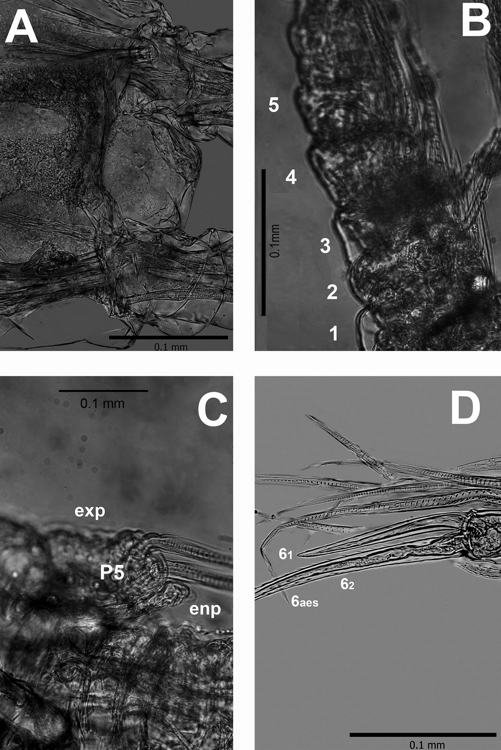
Figure 2. Monstrilla hendrickxi sp. n., from the Gulf of California, holotype female, digital photos. A, Anterior part of cephalothorax showing weakly produced forehead and lack of eyes; B, antennule showing dorsal segmentation; C, fifth leg (P5) showing exopodal (exp) and endopodal (enp) lobes, ventral view; D, apical elements (61, 62, and 6aes) of distal antennular segment.

Figure 3. Monstrilla hendrickxi sp. n., from the Gulf of California, holotype female. A, Antennule showing setation labelled in accordance with Grygier and Ohtsuka’s (1995) nomenclature, ventral view; B, similarly labelled setation of second antennular segment, ventral view, also showing segment’s inner distal conical process (arrow); C, distal (fifth) segment of antennule, ventral view, showing similarly labelled setation and distal process (arrow); D, anterior third of cephalothorax, ventral view, showing integumental ornamentation, including nipple-like processes (nlp), anterior pore cluster (apc), and preoral pores (pp). Scales A-D = 100 µm.

Figure 4. Monstrilla hendrickxi sp. n., from the Gulf of California, holotype female. A, Urosome, ventral view, showing bilobed fifth leg with exopodal (exp) and endopodal (enp) lobes, ovigerous spines (os), and caudal rami setation (I-VI); B, anterior half of cephalothorax, ventral view, showing unlayed internal egg mass (em), oral cone (oc), and nipple-like processes (nlp); C, antennule segments 1-3 (S1-S3), ventral view, showing setation labelled in accordance with Grygier and Ohtsuka’s (1995) nomenclature, including modified setae IIIv and IIId; D, right leg 1, semi-lateral view, showing setation including basipodal seta (bs) and exopodal (exp) and endopodal (enp) rami. Scales A-D = 100 µm.
Taxonomic summary
Type locality. Southern Gulf of California, Mexico (25°53’15” N, 110°10’08” W). Sampling depth between 710 and 750 m.
Material examined. One subadult female (holotype), partially dissected and mounted on 2 semi-permanent glycerin slides sealed with acrylic nail varnish (ECO-CH-Z 11860). Epibenthic sledge, TALUD XVI B cruise, southern Gulf of California, Mexico, 31 May 2014.
Etymology. The specific name, a masculine genitive eponym, honors Dr. Michel E. Hendrickx (ICMyL-UNAM) for his sustained efforts and achievements in exploring the crustacean fauna of the Gulf of California and the Mexican Pacific.
Male. Unknown.
Host. Unknown.
Remarks
The sampling gear used to collect this specimen was an epibenthic sledge, not a plankton net; the latter is more efficient for capturing planktonic adult monstrilloids in surface waters. Epi-mesopelagic monstrilloids collected by sledge type gears have been reported from depths of 118 and 302 m in the North Atlantic (Suárez-Morales & Mercado-Salas, 2023), but those individuals were badly damaged even though the sledge had an attached plankton collector (Brandt et al., 2014). The specimen recovered from the TALUD XVI-B sledge sample was in reasonably good condition for taxonomic study.
The present subadult female monstrilloid from the Gulf of California can be readily assigned to the genus Monstrilla by its possession of the diagnostic generic features for females, including the presence of 2 somites between the genital double-somite and the anal somite, 6 caudal setae, and the oral cone’s location ventrally at nearly mid-length of the cephalothorax (Isaac, 1975; Suárez-Morales, 1994a). Among the species-level diagnostic features of M. hendrickxi sp. n., the most useful for comparison among congeneric species are the antennular structure and armature, the shape of leg 5, and the absence of eyes. These will be considered in sequence below.
The specifically distinctive characters of M. hendrickxi sp. n. include: 1) eyes and eye-related structures absent; 2) antennules relatively short, robust, representing nearly 33% of cephalothorax length, with segments 2-5 partly fused; 3) segments 2-5 furnished with modified setae or strong spiniform processes, 4) fifth antennulary segment with remarkably long, thick apical elements; 5) fifth leg bilobed, with digitiform endopodal lobe unarmed, exopodal lobe with 2 terminal setae; 6) 6 caudal setae, innermost seta (VI) being shortest, proximal outer seta (I) longest. The finding of subadult monstrillids in the plankton is not unusual and some species have been described from these individuals, including the first described monstrilloid copepod, Thaumaleus typica (Krøyer, 1842) (Grygier, 1994), Monstrilla capitellicola Hartman (1961), M. elongata Suárez-Morales, 1994a, and Monstrilla sp. from Hawaii (Suárez-Morales et al., 2014).
Partial or complete fusion of antennular segments 2-5 is found in several other species of Monstrilla, including M. ilhoii Lee & Chang, 2016, M. mariaeugeniae Suárez-Morales & Islas-Landeros, 1993, M. satchmoi Suárez-Morales & Dias, 2001, M. grandis Giesbrecht, 1891, M. gracilicauda Giesbrecht, 1893, and M. elongata Suárez-Morales, 1994a. None of these species displays the remarkable development of apical elements 61, 62, and 6aes observed in M. hendrickxi sp. n. The only available illustration of an antennule of M. nichollsi Davis, 1949 (= C. helgolandica) (Suárez-Morales pers. obs.) (cf. Nicholls, 1944: fig. 26, as Monstrilla sp.) shows a very long apical element on its fifth segment, which is probably identifiable as the aesthetasc 6aes. Elsewhere on the antennule, no congeneric species has modified setal elements IIId and IIIv on segment 3 or large, spiniform or conical processes on segments 2, 4, and 5 like those described in the new species.
Only a few known species originally described as Monstrilla possess a bilobed fifth leg with 2 setae on the outer (exopodal) lobe, 2 of them have been transferred to the genus Caromiobenella: C. helgolandica (Claus, 1863) and C. hamatapex (Grygier & Ohtsuka, 1995); the other species of Monstrilla sharing this character are M. mariaeugeniae, M. capitellicola, and M. leucopis Sars, 1921. Also, both Monstrilla sp. from Hawaii and M. capitellicola from Southern California (Hartman, 1961), likely represented by subadult individuals, also show only 2 setae on the outer lobe, a character conserved through the copepodiid stages CIII-V (Suárez-Morales et al., 2014). The new species M. hendrickxi differs from C. helgolandica, C. hamatapex, M. capitellicola, and M. leucopis, by its possession of a long, digitiform endopodal lobe, which is absent in these 4 species (Chang, 2014; Grygier & Ohtsuka, 1995; Sars, 1921; Zavarzin & Suárez-Morales, 2024). The corresponding endopodal lobe is clearly shorter in M. capitellicola (Hartman, 1961) than in the new species. Monstrilla wandelii Stephensen, 1913, and M. mariaeugeniae both exhibit a small, unarmed subtriangular endopodal lobe (Nicholls, 1944, fig 26; Park, 1967; Suárez-Morales & Islas-Landeros, 1993), which clearly differs from the elongate, digitiform endopodal lobe observed in M. hendrickxi sp. n.. Monstrilla nichollsi, a synonym of C. helgolandica (Suárez-Morales pers. obs.), was named by Davis (1949) based solely on Nicholl’s (1944, fig. 26) illustration of the fifth leg, thus allowing us to add C. helgolandica to the group of monstrillid species with 2 exopodal setae on the fifth leg exopodal lobe. It should be noted that the armature of the fifth leg exopodal lobe is conservative during the immature stages including the preadult CV (Suárez-Morales et al., 2014); changes in this character at the final molt are unlikely.
Monstrilla hendrickxi sp. n. is the only monstrilloid copepod in which no trace of the naupliar eye is present, although weakly developed visual structures have been observed previously in deep-living species (Suárez-Morales & Mercado-Salas, 2023). This contrasts with the usually well-developed, highly pigmented, three-cup naupliar eyes of most known monstrilloids. Functional eyes are probably extremely important for planktonic adult monstrilloids, allowing them, for example, to migrate to different light conditions in the water column and favor their dispersal (Suárez-Morales, 2018; Suárez-Morales & Gasca, 1990). The weak eye development of deep-living monstrilloids is likely an adaptive consequence of their aphotic habitat.
Monstrilla hendrickxi sp. n. is the fifth species of the copepod order Monstrilloida recorded from the Gulf of California, after Monstrilla gibbosa Suárez-Morales & Palomares-García, 1995, Spinomonstrilla spinosa (Park, 1967) (originally reported as Monstrilla spinosa), Cymbasoma californiense Suárez-Morales & Palomares-García, 1999, and recently M. leucopis Sars, 1921 (Suárez-Morales, 2019; Suárez-Morales & Palomares-García, 1999; Suárez-Morales & Velázquez-Ornelas, 2023).
Acknowledgements
We thank Michel E. Hendrickx (ICMyL-UNAM) for kindly allowing us to examine this specimen. Ship time for the TALUD XVI-B cruise was provided by the Coordinación de la Investigación Científica, UNAM, and partly supported by Conacyt (project # 179467). We also thank to an anonymous reviewer for the corrections made to improve this article.
References
Brandt, A., Havermans, C., Janussen, D., Jörger, K. M., Meyer-Löbbecke, A., Schnurr, S. et al. (2014). Composition and abundance of epibenthic-sledge catches in the South Polar Front of the Atlantic. Deep-Sea Research II, 108, 69–75. Doi?
Claus, C.(1863). Die frei lebenden Copepoden mit besonderer Berücksichtigung der Fauna Deutschlands, der Nordsee und des Mittelmeeres. Leipzig: Verlag von Wilhelm Engelmann.
Chang, C. Y. (2014). Two new records of monstrilloid copepods (Crustacea) from Korea. Animal Systematics, Evolution and Diversity, 30, 206–214. https://doi.org/10.5635/ASED.
2014.30.3.206
Cruz-Lopes da Rosa, J., Dias, C. O., Suárez-Morales, E., Weber, L. I., & Gomes-Fischer, L. (2021). Record of Caromiobenella (Copepoda, Monstrilloida) in Brazil and discovery of the male of C. brasiliensis: morphological and molecular evidence. Diversity, 13, 241. https://doi.org/
10.3390/d13060241
Dana, J. D. (1849). Conspectus crustaceorum, quae in orbis terrarum circumnavigatione, Carolo Wilkes, e classe Reipublicae foederatae duce, lexit et descripsit Jacobus D. Dana. Pars II. Proceedings of the American Academy of Arts and Sciences, 2, 9–61.
Davis, C. C. (1949). A preliminary revision of the Monstrilloida, with descriptions of two new species. Transactions of the American Microscopical Society, 68, 245–255. https://doi.org/10.2307/3223221
Giesbrecht, W. (1891). Elenco dei Copepodi pescati dalla R. Corvetta ‘Vettor Pisani’ secondo la loro distribuzione geografica. Atti della Accademia Nazionale dei Lincei, Classe di Scienze Fisiche Matematiche e Naturali Rendiconti, 4, 276–282.
Giesbrecht, W. (1893). Systematik und Faunistik der pelagischen Copepoden des Golfes von Neapel und der angrenzenden Meeres-Abschnitte. Fauna und Flora des Golfes von Neapel und der angrenzenden Meeres-Abschnitte, 19, 1–831.
Grygier, M. J. (1994) [dated 1993]. Identity of Thaumatoessa (= Thaumaleus) typica Krøyer, the first described monstrilloid copepod. Sarsia, 78, 235–242. https://doi.org/10.1080/00364827.1993.10413537
Grygier, M. J., & Ohtsuka, S. (1995). SEM observation of the nauplius of Monstrilla hamatapex, new species, from Japan and an example of upgraded descriptive standards for monstrilloid copepods. Journal of Crustacean Biology, 15, 703–719. https://doi.org/10.1163/193724095X00118
Grygier, M. J., & Ohtsuka, S. (2008). A new genus of monstrilloid copepods (Crustacea) with anteriorly pointing ovigerous spines and related adaptations for subthoracic brooding. Zoological Journal of the Linnean Society, 152, 459–506. https://doi.org/10.1111/j.1096-3642.2007.00381.x
Hartman, O. (1961). A new monstrillid copepod parasitic in capitellid polychaetes in southern California. Zoologischer Anzeiger, 167, 325–334.
Huys, R., & Boxshall, G. A. (1991). Copepod evolution. London: Ray Society.
Huys, R., Llewellyn-Hughes, J., Conroy-Dalton, S., Olson, P. D., Spinks, J. N., & Johnston, D. A. (2007). Extraordinary host switching in siphonostomatoid copepods and the demise of the Monstrilloida: Integrating molecular data, ontogeny and antennulary morphology. Molecular Phylogenetics
and Evolution, 43, 368–378. https://doi.org/10.1016/j.ympev.
2007.02.004
Isaac, M. J. (1975). Copepoda, sub-order: Monstrilloida. Fiches d’Identification du Zooplancton, 144/145, 1–10.
Jeon, D., Lee, W., & Soh, H. Y. (2018). New genus and two new species of monstrilloid copepods (Copepoda: Monstrillidae): integrating morphological, molecular phylogenetic, and ecological evidence. Journal of Crustacean Biology, 38, 45–65. https://doi.org/10.1093 /jcbiol/rux095
Jeon, D., Lim, D., Lee, W., & Soh, H. Y. (2016). First use of molecular evidence to match sexes in the Monstrilloida (Crustacea: Copepoda), and taxonomic implications of the newly recognized and described partly Maemonstrilla-like females of Monstrillopsis longilobata Lee, Kim & Chang, 2016. Peer J, 13,e4938. https://doi.org/10.7717/peerj.4938
Krøyer, H. (1842). Crustacés. In P. E. Gaimard (Ed.), Atlas de Zoologie. Voyages de la Commission Scientifique du Nord en Scandinavie, en Laponie au Spitzberg et aux Feröe pendant les Anneés 1838, 1839 et 1840 sur la Corvette La Recherche, Commandée par M. Fabvre (pl. 41–43). Arthus Bertrand, Paris.
Lee, J., & Chang, C. Y. (2016). A new species of Monstrilla Dana, 1849 (Copepoda: Monstrilloida: Monstrillidae) from Korea, including a key to species from the North-west Pacific. Zootaxa, 4174, 396–409. https://doi.org/10.11646/zootaxa.4174.1.24
Nicholls, A. G. (1944). Littoral Copepoda from South Australia (II) Calanoida, Cyclopoida, Notodelphyoida, Monstrilloida, and Caligoida. Records of the South Australian Museum, 8, 1–62.
Park, T. S. (1967). Two unreported species and one new species of Monstrilla (Copepoda: Monstrilloida) from the Strait of Georgia. Transactions of the American Microscopical Society, 86, 144–152.
Razouls, C., Desreumaux, N., Kouwenberg, J., & de Bovée, F. (2023). Biodiversity of marine planktonic copepods (morphology, geographic distribution, and biological data [2005-2023]). Sorbonne University, CNRS. http://copepodes.obs-banyuls.fr/en [Accessed April 28, 2022]
Sale, P. F, McWilliams, P. S., & Anderson, D. T. (1996). Composition of the near-reef zooplankton at Heron Reef, Great Barrier Reef. Marine Biology, 34, 59–66. https://doi.org/10.1007/BF00390788
Sars, G. O. (1901). An account of the Crustacea of Norway with short descriptions and figures of all the species Vol. IV. Copepoda Calanoida. Bergen: The Bergen Museum.
Sars, G. O. (1921). An account of the Crustacea of Norway with short descriptions and figures of all the species, Vol. VIII. Copepoda Monstrilloida & Notodelphyoida. Bergen: The Bergen Museum.
Stephensen, K. (1913) Account of the Crustacea and the Pycnogonida collected by Dr. V. Nordmann in the summer of 1911 from northern Stromfjord and Giesecke Lake in West Greenland. Meddeleser om Groenland, 51, 55–77.
Suárez-Morales, E. (1994a). Monstrilla elongata, a new monstrilloid copepod (Crustacea: Copepoda: Monstrilloida) from a reef lagoon of the Caribbean coast of Mexico. Proceedings of the Biological Society of Washington, 107, 262–267.
Suárez-Morales, E. (1994b). Thaumaleus quintanarooensis, a new monstrilloid copepod from the Mexican coasts of the Caribbean Sea. Bulletin of Marine Science, 54, 381–384.
Suárez-Morales, E. (2001). An aggregation of monstrilloid copepods in a western Caribbean reef area: ecological and conceptual implications. Crustaceana, 74, 689–696. https://doi.org/10.1163/156854001750377966
Suárez-Morales, E. (2011). Diversity of the Monstrilloida (Crustacea: Copepoda). Plos One, 6, e22915. https://doi.org/10.1371/journal.pone.0022915
Suárez-Morales, E. (2018). Monstrilloid copepods: the best of three worlds. Bulletin of the Southern California Academy of Sciences, 107, 92–103. https://doi.org/10.22201/ib.20078706e.2020.91.3176
Suárez-Morales, E. (2019). A new genus of the Monstrilloida (Copepoda) with large rostral process and metasomal spines, and redescription of Monstrilla spinosa Park, 1967. Crustaceana, 92, 1099–1112. https://doi.org/10.1163/
15685403-00003925
Suárez-Morales, E., & Dias, C. O. (2001). Taxonomic report of some monstrilloids (Copepoda: Monstrilloida) from Brazil with description of four new species. Bulletin de l’Institut Royal des Sciences Naturelles de Belgique Biologie, 71, 65–81.
Suárez-Morales, E., & Gasca, R. (1990). Variación dial del zooplancton asociado a las praderas de Thalassia testudinum en una laguna arrecifal del Caribe Mexicano. Universidad y Ciencia, 7, 57–64.
Suárez-Morales, E., Harris, L. H., Ferrari, F. D., & Gasca, R. (2014). Late postnaupliar development of Monstrilla sp. (Copepoda: Monstrilloida), a protelean endoparasite of benthic polychaetes. Invertebrate Reproduction & Development, 58, 60–73.
Suárez-Morales, E., & Islas-Landeros, M. E. (1993). A new species of Monstrilla (Copepoda: Monstrilloida) from a reef lagoon off the Mexican coast of the Caribbean Sea. Hydrobiologia, 271, 45–48.
Suárez-Morales, E., & McKinnon, A. D. (2014). The Australian Monstrilloida (Crustacea: Copepoda) I. Monstrillopsis Sars, Maemonstrilla Grygier & Ohtsuka, and Australomonstrillopsis gen. nov. Zootaxa, 3779, 301–340. https://doi.org/10.11646/zootaxa.3779.3.1
Suárez-Morales, E., & McKinnon, A. D., (2016). The Australian Monstrilloida (Crustacea: Copepoda) II. Cymbasoma Thompson, 1888. Zootaxa Monographs, 4102, 1–129. https://doi.org/10.11646/zootaxa.4102.1.1
Suárez-Morales, E., & Mercado-Salas, N. F. (2023). Two new species of Cymbasoma (Copepoda: Monstrilloida: Monstrillidae) from the North Atlantic. Journal of Natural History, 57, 1312–1330. https://doi.org/10.5852/ejt.
2024.917.2395
Suárez-Morales, E., Paiva Scardua, M., & Da Silva, P. M. (2010). Occurrence and histopathological effects of Monstrilla sp. (Copepoda: Monstrilloida) and other parasites in the brown mussel Perna perna from Brazil. Journal of the Marine Biological Association of the United Kingdom, 90, 953–958. https://doi.org/10.1017/S0025315409991391
Suárez-Morales, E., & Palomares-García, R. (1995). A new species of Monstrilla (Copepoda: Monstrilloida) from a coastal system of the Baja California Peninsula, Mexico. Journal of Plankton Research, 17, 745–752. https://doi.org/
10.1093/plankt/17.4.745
Suárez-Morales, E., & Palomares-García, R. (1999). Cymbasoma californiense, a new monstrilloid (Crustacea: Copepoda: Monstrilloida) from Baja California, Mexico. Proceedings of the Biological Society of Washington, 112, 189–198.
Suárez-Morales, E., Vásquez-Yeomans, L., & Santoya, L. (2020). A new species of the Cymbasoma longispinosum species-group(Copepoda, Monstrilloida, Monstrillidae) from Belize, western Caribbean Sea. Revista Mexicana de Biodiversidad, 91, e913176. https://doi.org/10.22201/ib.
20078706e.2020.91.3176
Suárez-Morales, E., & Velázquez-Ornelas, K. E. (2023). First record of Monstrilla leucopis G.O. Sars, 1921 (Copepoda: Monstrilloida: Monstrillidae) from the Eastern Pacific. Crustaceana, 96, 1183–1190. https://doi.org/10.1163/156854
03-bja10334
Thompson, I. C. (1888). Copepoda of Madeira and the Canary Islands, with descriptions of new genera and species. Zoological Journal of the Linnean Society, 20, 145–156. https://doi.org/10.1111/j.1096-3642.1888.tb01443.x
Walter, T. C., & Boxshall, G. A. (2022). World of copepods database Cymbasoma Thompson I.C., 1888. Accessed through: World Register of Marine Species (WoRMS)at: https://www.marinespecies.org/aphia.php?p=taxdetails&id=119778 on 2022-04-23
Zavarzin, D., & Suárez-Morales, E. (2024). First record of Caromiobenella helgolandica (Claus, 1863) (Copepoda: Monstrilloida: Monstrillidae) from the Okhotsk Sea. Crustaceana, 97, 151–157. https://doi.org/10.1163/15685403-
bja10345

A new species of Aleuropleurocelus (Hemiptera: Aleyrodidae) and key to the ceanothi group from Mexico
Vicente Emilio Carapia-Ruiz*
Universidad Autónoma del Estado de Morelos, Escuela de Estudios Superiores de Xalostoc, Av. Nicolas Bravo s/n, 62740 Xalostoc, Morelos, Mexico
*Corresponding author: vicente.carapia@uaem.mx (V.E. Carapia-Ruiz)
Received: 25 February 2024; accepted: 24 June 2024
http://zoobank.org/urn:lsid:zoobank.org:pub:4751138D-9FD4-4095-A858-3A6A4F6B8A47
Abstract
A new species of whitefly, Aleuropleurocelus tecomastans, is described. The studied specimens were found in the municipality of Acapulco, State of Guerrero, Mexico on Tecoma stans (L.) (Bignoniaceae) leaves. A dichotomous key to identify members of Aleuropleurocelus group ceanothi, defined by a transverse suture of the molt which reaches the submarginal line, is provided. Photographs of morphological pupal structures are given and diagnostic separation to other related species is discussed.
Keywords: Aleyrodinae; Aleuropleurocelus ceanothi; Whitefly
© 2024 Universidad Nacional Autónoma de México, Instituto de Biología. Este es un artículo Open Access bajo la licencia CC BY-NC-ND
(http://creativecommons.org/licenses/by-nc-nd/4.0/).
Una especie nueva de Aleuropleurocelus (Hemiptera: Aleyrodidae) y clave para el grupo ceanothi de Mexico
Resumen
Una especie nueva de mosca blanca, Aleuropleurocelus tecomastans, es descrita. Los especímenes estudiados fueron encontradosen el municipio de Acapulco, Estado de Guerrero, México sobre Tecoma stans (L.) (Bignoniaceae). Se provee una clave dicotómica para identificación de especies de Aleuropleurocelus grupo ceanothi, definido por una sutura transversa de la muda que termina en la línea submarginal. Se proporcionan fotografías de las estructuras morfológicas del pupario y se analiza la separación diagnóstica en otras especies relacionadas.
Palabras clave: Aleyrodinae; Aleuropleurocelusceanothi; Mosca blanca
Introduction
The genus Aleuropleurocelus was described by Drews and Sampson (1956), comprising 8 species and an identification key to all Californian species was included (Drews & Sampson, 1958). Later Dooley et al. (2010) described A. nevadensis Dooley, while Polaszek and Gill (2011) added A. hyptisemoryi Gill to the genus. Nowadays, 19 species of Mexican species of Aleuropleurocelus are known and have been largely studied by Carapia-Ruiz (2023), Carapia-Ruiz (2020a, b), Carapia-Ruiz and Sánchez-Flores (2019a, b), Carapia-Ruiz et al. (2018a, b, 2020, 2023), Sánchez-Flores and Carapia-Ruiz (2018a, b), Sánchez-Flores et al. (2018a, b, 2020, 2021). The genus is segregated into 3 major groups: abnormis (semioval), nigrans, and ceanothi according to Dooley et al. (2010) and Sánchez-Flores et al. (2021).
The ceanothi group, in which the transverse suture of molt ends at the submarginal line is included, A. granulata (Sampson & Drews), and the morphologically related species A. sampsoni Sánchez-Flores & Carapia-Ruiz and A. pseudogranulata Carapia-Ruiz & Sánchez-Flores. While collecting puparia of Aleyrodidae in Acapulco Guerrero, an unknown species of this group with distinctive characters was found. The objective of this contribution is to describe a new species and provide a key to all species of Aleuropleurocelus group ceanothi.
Materials and methods
The specimens were collected on the underside of the leaves of Tecoma stans (L.). in Acapulco, Guerrero. The specimens once taken were retained ethanol and thus transferred to the Laboratorio de Entomología, Escuela de Estudios Superiores de Xalostoc of the Universidad Autónoma del Estado de Morelos, to be fully processed and mounted in permanent preparation with Canada balsam on slides for further study under stereomicroscope and facilitating identification following specialized literature such as Drews and Sampson (1958), Martin (2004, 2005), and Sanchez-Flores et al. (2021). After preparations, specimens were observed under a Motic BA 320 phase contrast optical microscope considering several magnifications: 4X 100X, 400X and 1,000X. The terminology used follows Drews and Sampson (1956) and Martin (2005). The studied specimens are deposited at Colección Nacional de Insectos (CNIN), Instituto de Biología, Universidad Nacional Autónoma de México. México City, Mexico.
Description
Aleuropleurocelus tecomastans n. sp. Carapia-Ruiz
(Figs. 1-9)
http://zoobank.org/urn:lsid:zoobank.org:act:113654EB-09
53-4C95-9CFB-3FFFF8B3F8BE
Diagnosis. Pupa boat-shaped, transverse molting suture reaches the submarginal line, dorsum and venter black, eye spots with tubercles, abdominal depressions present, middle area of abdominal segments smooth, abdominal VIII setae anterolateral to the vasiform orifice very small.
General form: pupae in situ. Dorsal and ventral surface of pupae black, a thin fringe of wax is distinguished around the body margin.
Specimens on slides: semioval body (Fig. 1). Deflexed submargin. Margin: with 61-68 pairs of marginal teeth with 2-3 acute terminal protrusions (Fig. 2), submargin with a regular band of small tubercles (Fig. 3); subdorsum: with a band of crescent tubercles (Fig. 4). Cephalothorax: longitudinal molting suture with a row of defined tubercles on each side giving the appearance of a zipper, transverse molting suture ends at the apparent margin (submarginal fold), well defined meso-metathoracic suture (Fig. 5), ocular markings (eye spots) indicated by pale coloration and 5-7 pairs of pale tubercles in the subdorsal area near the submarginal line, cephalic setae absent; mid thoracic zone with 2 pairs of setae, the mesothoracic and the metathoracic. Abdomen: dorsum with abdominal segments I-VIII clearly visible in the middle part (Fig. 6). With abdominal depressions in the middle area of the segments (Fig. 7), cuticle in the middle of the abdominal segments smooth. Vasiform orifice: elongated semicordiform (Fig. 8); elevated; operculum with 4 irregular longitudinal furrows and spinules at the apex, completely covering the lingula and most of the vasiform orifice, ring of the orifice defined in its anterior part, abdominal VIII setae anterolateral to the vasiform orifice very small, caudal protuberance developed. Pores, normally as follows: 8 pairs in the cephalic area, 6 on submedian area and 2 posterior to eye spots; 4 pairs in the mesothorax, 2 on submedian area and 2 in the subdorsal area of the mosothorax; medial area of abdominal segments I, III, V, VII with 2 pairs each segment, segment VIII with 2 pairs; subdorsal area of abdominal segments II, IV, V, with 2 pairs of pores in each segment (Fig. 9).
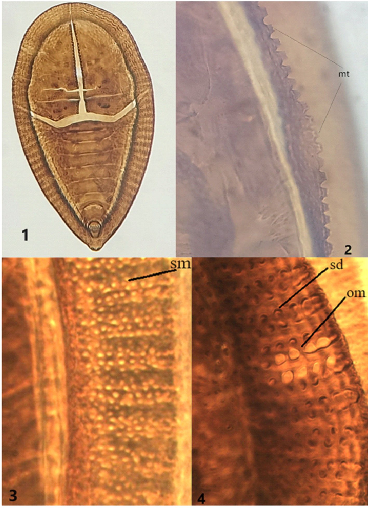
Figures 1-4. Aleuropleurocelus tecomastans.1) Puparium; 2) marginal teeth; 3) submarginal area; 4) subdorsal area. mt = Marginal teeth, om = ocular mark, sd = subdorsum, sm = submargin.
Venter: legs prothoracic, mesothoracic, metathoracic with apical adhesive sac, thoracic adhesive sacs near the base of the first pair of legs, base of the legs with a wide irregular band of 2-4 spinules, thoracic and abdomen cuticle smooth, well defined abdominal setae of segment VIII, posteriorly present a pair of spiracles. Chaetotaxy: a pair of anterior marginal setae present (near marginal teeth), cephalic setae absent, mesothoracic, metathoracic and caudal setae well developed, very small abdominal VIII setae, located anterolateral to the vasiform orifice, and posterior marginal setae small.
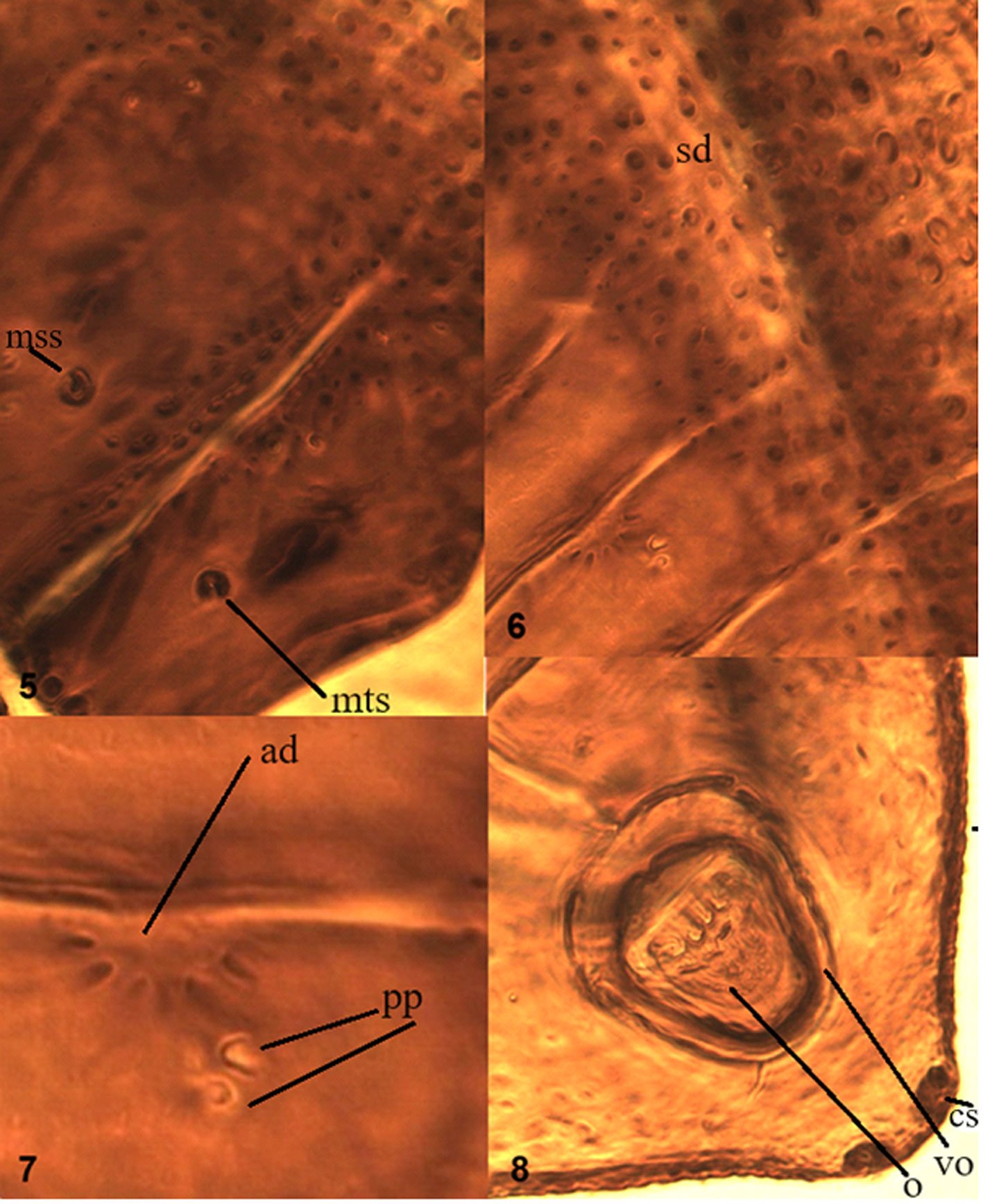
Figures 5-8. Aleuropleurocelus tecomastans.5) Thoracic area; 6) submedia and subdorsal area; 7) depression and pore of abdominal segment IV; 8) vasiform orifice. ad = Abdominal depression, cs = caudal seta, mss = mesothoracic seta, mts = metathoracic seta, o = operculum, pp = pore porete, sd = subdorsum, vo = vasiform orifice.
Measurements. Specimens on slides: body 550-650 µm long by 300-400 µm wide. Submargin approximately 45-55 μm. Cephalothorax: 230-280 μm, longitudinal molting suture, 240-360 μm, transverse molting suture 220-250 μm, the metathorax 30-45 μm long in its middle area, cephalic elongated structures of 8-10 µm long by 3-5 µm wide. Abdomen: abdominal segments length for segment I 22-26 μm, segment II 22-26 μm, segment III 25-30 μm, segment IV 26 -30 μm, segment V 27-32 μm, segment VI 26-29 μm, segment VII 23-27 μm, and segment VIII (from suture VII-VIII to vasiform orifice) 40-50 μm, distance from vasiform orifice to apparent margin 25-35 μm; abdominal depressions segments with approximate length in segment I 3-5 μm long by 10-12 μm wide, in segment II 3-4 μm long by 12-15 μm wide, in segment III 3-4 μm long by 10-13 μm wide, in segment IV 3-4 μm long by 10-14 μm wide, in segment V 5-7 μm long by 10-15 μm wide, in segment VI 5-6 μm long by 9-11 μm wide. Vasiform orifice: 46-50 µm long by 32-38 µm of broad at the widest part; operculum 25-30 μm long by 22-26 μm wide. Venter: Prothoracic legs 75-77 μm long, mesothoracic legs 75-78 μm long, metathoracic legs 85-89 μm long, thoracic adhesive sacs of 16-20 μm in diameter, base of the legs spinules 4 μm long and 2 μm wide. Setae: anterior marginal setae approximately 7 μm long, mesothoracic setae approximately 15 μm long, metathoracic setae approximately 20 μm long, abdominal VIII setae 3-4 μm long, caudal seta approximately 20 μm long, and posterior marginal seta approximately 10 μm long.
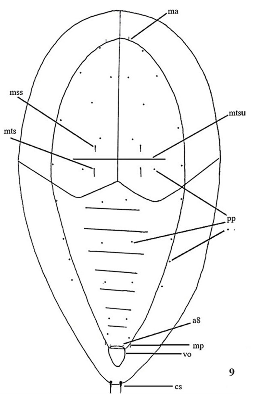
Figure 9. Aleuropleurocelus tecomastans. Pores and setae distribution. a8 = VIII abdominal segment seta, cs = caudal seta, ma = marginal anterior seta, mp = marginal posterior seta, mss = mesothoracic seta, mts = metathoracic seta, mtsu = metathoracic suture, pp = pore porete, vo = vasiform orifice.
Taxonomic summary
Type locality: northeast of Acapulco, Guerrero, Mexico
Type material: holotype, puparium: Acapulco, Guerrero, Mexico, in leaves of Tecoma stans (Bignoniaceae), 8-iv-2021, Col. V. E. Carapia-Ruiz, deposited in CNIN (Colección Nacional de Insectos, Instituto de Biología, Universidad Nacional Autónoma de México, Mexico City, Mexico), HOM-TIP-170. Paratypes: puparia, same data as holotype, 2 deposited in CNIN, HOM-PAR-171, HOM-PAR-172.
Etymology: the suffix name is based on a combination of the host plant’s scientific name where specimens were associated.
Distribution: Acapulco, Guerrero, Mexico.
Plant associations: Tecoma stans (Bignoniaceae).
Remarks.
Aleuropleurocelus tecomastans is placed within the ceanothi group by the transverse molting suture reaches the apparent margin (submarginal line). The new species is similar in apparence to A. granulate, A. sampsoni,and A. pseudogranulata but can be differentiated by the presence of abdominal depressions which is opposite as shown in A. granulata, A. sampsoni, A. pseudogranulata or A. ceanothi. Also A. asciculatus presents a subdorsal fold which is absent in the other species.
Key to species of Aleuropleurocelus group ceanothi
1. With bands of dense wax on dorsum, pores of double wall on dorsum 2
—Without such bands or pores 3
2. (1) Two bands of dense wax on dorsum (1 thin band on subdorsum and 1 wide band on submedian area ornatus Drews & Sampson
— One band of dense wax on subdorsum sampsoni Sánchez Flores & Carapia-Ruiz
3. (1) Tubercles on submedian surface absent 4
—Tubercles on submedian surface present 8
4. (3) Without evident tubercles on subdorsal surface 5
— With evident tubercles on subdorsal surface 6
5. (4) Longitudinal suture of the molt with tubercles on metathorax laingi Drews & Sampson
— Longitudinal suture of the molt without tubercles on metathorax coachellensis Drews & Sampson
6. (4) Subdorsal fold absent 7
— Subdorsal fold present asciculatus Carapia-Ruiz
7. (6) 2 pair of thoracic adhesive sacs, submarginal band with pores erigonium Carapia-Ruiz
— Without tubercles on the anterior and posterior part of the abdominal segments, abdominal depressions present tecomastans n. sp.
8. (3) With 2 pairs of thoracic adhesive sacs, submedian area with tubercles only on the anterior part of the abdominal segments; marginal teeth without 2 or more evident prostructions 9
— With a pair of thoracic adhesive sacs, submedian area with tubercles on the anterior and posterior part of the abdominal segments; marginal teeth with evident prostructions; transversal suture of the molt curved 10
9. (8) Half posterior of puparium in elliptic form sierra (Sampson)
— Half posterior of puparium in triangular form ceanothi (Sampson)
10. (8) Vasiform orifice semicircular, venter of abdomen with posterior area very narrow, transversal suture of the molt almost straight on median area granulata Sampson & Drews
— Vasiform orifice elongated, clearly more long than wide, venter of abdomen with posterior area triangular in form, transversal suture of the molt curved on median area pseudogranulata Carapia-Ruiz
Acknowledgments
To Paul Brawn and David Ovread of the British Museum of Natural History (BMNH) for facilitating a loan of Aleuropleurocelus to study the specimens.
References
Carapia-Ruiz, V. E. (2020a). Descripción de una especie nueva del género Aleuropleurocelus y nuevos registros para Baja California, México. Southwestern Entomologist, 45, 269–274. https://doi.org/10.3958/059.045.0128
Carapia-Ruiz, V. E. (2020b). Description of a new species of the genus Aleuropleurocelus Drews & Sampson (Hemiptera: Aleyrodidae) and a new country record for a species of the genus from Mexico. Acta Zoológica Mexicana (nueva serie), 36, 1–7. https://doi.org/10.21829/azm.2020.3612184
Carapia-Ruiz, V. E. (2023). Dos especies nuevas de Aleuro-
pleurocelus de México, Southwestern Entomologist, 48, 641-648. https://doi.org/10.3958/059.045.0425
Carapia-Ruiz, V. E., & Sánchez-Flores, O. A. (2019a). Descripción de una especie nueva del género Aleuropleurocelus Drews y Sampson (Hemiptera: Aleyrodidae) de California, Estados Unidos. Acta Zoológica Mexicana (nueva serie), 35, 1–4. https://doi.org/10.21829/azm.2019.3501230
Carapia-Ruiz, V. E., & Sánchez-Flores, O. A. (2019b). Descripción de la primera especie pálida del género Aleuropleurocelus. Southwestern Entomologist, 44, 315–319. https://doi.org/10.3958/059.044.0133
Carapia-Ruiz, V. E., Sánchez-Flores, O. A., & García-Ochaeta, J. F. (2023). A new whitefly species, Aleuropleurocelus petenensis sp. nov. (Hemiptera: Aleyrodidae), from Guatemala. Acta Zoológica Mexicana (nueva serie), 39, 1–8. https://doi.org/10.21829/azm.2023.3912470
Carapia-Ruiz, V. E., Sánchez-Flores, O. A., García-Martínez, O., & Castillo-Gutiérrez, A. (2018a). Descripción de dos especies nuevas del género Aleuropleurocelus Drews y Sampson, 1956 (Hemiptera: Aleyrodidae) de México. Insecta Mundi, 0606, 1–13.
Carapia-Ruiz, V. E., Sánchez-Flores, O. A., García-Martínez, O., & Castillo-Gutiérrez, A. (2018b). Descripción de dos especies nuevas del género Aleuropleurocelus Drews y Sampson, 1956 (Hemiptera: Aleyrodidae) de México. Southwestern Entomologist, 43, 517–526.
Carapia-Ruiz, V. E., Sánchez-Flores, O. A., García-Martínez, O., & Castillo-Gutiérrez, A. (2021). Aleuropleurocelus palidonigrans sp. nov. de Guerrero, México, Southwestern Entomologist, 46, 781–786. https://doi.org/10.3958/059.046.
0320
Dooley, J. W., Lambrecht, S., & Honda, J. (2010). Eight new state records of aleyrodine whiteflies found in Clark County, Nevada and three newly described taxa (Hemiptera: Aleyrodidae, Aleyrodinae). Insecta Mundi, 140, 1−36.
Drews, E. A., & Sampson, W. W. (1956). Tetralicia and a new related genus Aleuropleurocelus (Homoptera: Aleyrodidae). Annals Entomological Society of America, 49, 280–283. https://doi.org/10.1093/aesa/49.3.280
Drews, E. A., & Sampson, W. W. (1958). California aleyrodids of the genus Aleuropleurocelus. Annals of the Entomological Society of America, 51, 120–125.
Martin, J. H. (2004). The whiteflies of Belize (Hemiptera: Aleyrodidae) Part 1 — Introduction and account of the subfamily Aleurodicinae Quaintance and Baker. Zootaxa, 681, 1–119. https://dx.doi.org/10.11646/zootaxa.681.1.1
Martin, J. H. (2005). Whiteflies of Belize (Hemiptera: Aleyrodidae). Part 2 — A review of the subfamily Aleyrodinae Westwood. Zootaxa, 1098, 1–116. https://dx.
doi.org/10.11646/zootaxa.1098.1.1
Polaszek, A., & Gill, R. (2011). A new species of whitefly (Hemiptera: Aleyrodidae) and its parasitoid (Hymenoptera: Aphelinidae) from desert lavender in California. Zootaxa, 2750, 51–59. https://doi.org/10.11646/zootaxa.2150.1.5/biota
xa.org
Sánchez-Flores, O. A., & Carapia-Ruiz, V. E. (2018a). Nueva especie de Aleuropleurocelus Drews y Sampson (Hemiptera: Aleyrodidae) y clave para especies del grupo de forma oval. Insecta Mundi, 651, 1–12.
Sánchez-Flores, O. A., & Carapia-Ruiz, V. E. (2018b). Description of two new species of the genus Aleuropleurocelus Drews y Sampson (Hemiptera: Aleyrodidae) from Mexico. Acta Zoológica Mexicana (nueva serie), 34, 1–9. https://doi.org/10.21829/azm.2018.3412145
Sánchez-Flores, O. A., Carapia-Ruiz, V. E., Coronado-Blanco, J. M., & Ruíz-Cancino, E. (2020). Description of Aleuropleurocelus sampsoni sp. nov. (Hemiptera: Aleyrodidae) from Tamaulipas, Mexico. Florida Entomologist, 103, 274–280. https://doi.org/10.1653/024.103.0219
Sánchez-Flores, O. A., Carapia-Ruiz, V. E., García-Martínez, O., & Castillo-Gutiérrez, A. (2018a). Descripción de una especie nueva del género Aleuropleurocelus de México. Southwestern Entomologist, 43, 257–262. https://doi.org/
10.3958/059.043.0116
Sánchez-Flores, O. A., Carapia-Ruiz, V. E., García-Martínez, O., & Castillo-Gutiérrez, A. (2018b). Descripción de una especie nueva del género Aleuropleurocelus (Hemiptera: Aleyrodidae) de México. Acta Zoológica Mexicana (nueva serie), 34, 1–6. https://doi.org/10.21829/azm.2018.3412104
Sánchez-Flores, O. A., García-Ochaeta, J. F., Carapia-Ruiz, V. E., Ruiz-Cancino, E., & Coronado-Blanco, J. M. (2021). New species of Aleuropleurocelus Drews and Sampson (Hemiptera: Aleyrodidae) from Guatemala, with a key to species from the oval group. Proceedings of the Entomological Society of Washington, 123, 615–621. https://doi.org/10.4289/0013-8797.123.3.614

A multigene approach to identify the scorpion species (Arachnida: Scorpiones) of Colima, Mexico, with comments on their venom diversity
Edmundo González-Santillán a, Laura L. Valdez-Velázquez b, *, Ofelia Delgado-Hernández c, Jimena I. Cid-Uribe d, María Teresa Romero-Gutiérrez e, Lourival D. Possani d
a Universidad Nacional Autónoma de México, Instituto de Biología, Departamento de Zoología, Colección Nacional de Arácnidos, Tercer Circuito Exterior s/n, Ciudad Universitaria, Coyoacán, 04510 Ciudad de México, Mexico
b Universidad de Colima, Facultad de Ciencias Químicas y Facultad de Medicina, Km 9 Carretera Colima-Coquimatlán, 28400 Coquimatlán, Colima, Mexico
c Instituto Francisco Possenti, Av. Toluca 621, Olivar de los Padres, Álvaro Obregón, 01780 Mexico City, Mexico
d Universidad Nacional Autónoma de México, Instituto de Biotecnología, Avenida Universidad 2001, Colonia Chamilpa, 62210 Cuernavaca, Morelos, Mexico
e Universidad de Guadalajara, Centro Universitario Tlajomulco, Departamento de Innovación Tecnológica, Carretera Tlajomulco – Santa Fé Km. 3.5 No.595 Lomas de Tejeda, 45641 Tlajomulco de Zúñiga, Jalisco, Mexico
*Corresponding author: lauravaldez@ucol.mx (L.L. Valdez-Velázquez)
Received: 9 October 2023; accepted: 19 March 2024
Abstract
Scorpion species diversity in Colima was investigated with a multigene approach. Fieldwork produced 34 lots of scorpions that were analyzed with 12S rDNA, 16S rDNA, COI, and 28S rDNA genetic markers. Our results confirmed prior phylogenetic results recovering the monophyly of the families Buthidae and Vaejovidae, some species groups, and genera. We recorded 11 described species of scorpions and found 3 putatively undescribed species of Centruroides, 1 of Mesomexovis, and 1 of Vaejovis. Furthermore, we obtained evidence that Centruroides elegans, C. infamatus,and C. limpidus do not occur in Colima, contrary to prior reports. Seven genetically different and medically relevant species of Centruroides for Colima are recorded for the first time. We used the InDRE database (Instituto de Diagnóstico y Referencia Epidemiológicos), which contains georeferenced points of scorpions, to estimate the distribution of the scorpion species found in our fieldwork. Finally, we discuss from a biogeographical, ecological, and medical point of view the presence and origin of the 14 scorpion species found in Colima.
Keywords: Barcoding; Holotype; Medical relevance; Microendemic; New species; Species group; Substrate-specialist
© 2024 Universidad Nacional Autónoma de México, Instituto de Biología. Este es un artículo Open Access bajo la licencia CC BY-NC-ND
(http://creativecommons.org/licenses/by-nc-nd/4.0/).
Una aproximación multigenes para identificar a las especies de alacranes (Arachnida: Scorpiones) de Colima, México, con cometarios sobre la diversidad de sus venenos
Resumen
La diversidad de especies de alacranes de Colima se investigó utilizando una aproximación multigenes. Del trabajo de campo se obtuvieron 34 lotes de alacranes que fueron analizados con los marcadores 12S rDNA, 16S rDNA, COI, y 28S rDNA. La comparación con trabajos de filogenia previos nos permitió confirmar la monofilia de las familias Buthidae y Vaejovidae, de algunos grupos de especies y géneros. Encontramos 11 especies de alacranes descritas, 3 putativamente nuevas de Centruroides, 1 de Mesomexovis y 1 de Vaejovis. También obtuvimos evidencia de que Centruroides elegans, C. infamatus y C. limpidus no están distribuidos en Colima, como se registró en trabajos anteriores. Reportamos 7 especies genéticamente distintas y de importancia médica para Colima. Usamos la base de datos del InDRE (Instituto de Diagnóstico y Referencia Epidemiológicos) que contiene puntos georreferenciados de alacranes para estimar la distribución de las especies que recolectamos en el campo. Finalmente, discutimos desde una perspectiva biogeográfica, ecológica y de importancia médica las 14 especies de alacranes que reportamos para Colima.
Palabras clave: Código de barras; Holotipo; Importancia médica; Microendémico; Especie nueva; Grupo de especies; Sustrato-especialista
Introduction
The knowledge of scorpion diversity in North America has improved recently (González-Santillán & Prendini, 2013; Goodman, Prendini, Francke et al., 2021; Ponce-Saavedra & Francke, 2019; Santibáñez-López et al., 2014); however, much remains to be discovered. Local-scale inventories may be a solution to unveil species communities that, in turn, can help conform regional faunas. This approach has rarely been applied to study scorpion diversity. Furthermore, few local faunal studies have been conducted in Mexico, and only a handful of them have been published; other revisionary contributions included limited fieldwork effort (Baldazo-Monsivais et al., 2012, 2016, 2017).
The International Barcode of Life (iBOL) has grown as a powerful tool for discovering biodiversity, among other applications (https://ibol.org). Scorpion barcoding studies have permitted the identification and delimitation of species in several regions of the world (Fet et al., 2014, 2016; Goodman, Prendini, & Esposito, 2021; Podnar et al., 2021). Despite the high diversity of scorpions in Mexico —an update by Ponce-Saavedra et al. (2023) comprises 311 scorpion species— only 1 mini-barcoding study has been conducted (Goodman, Prendini, & Esposito, 2021). Herein, we present a second scorpion barcoding study for this country but aim at discovering the components of a local scorpion assembly. Colima exhibits a complex topology comprising littorals with a tropical climate and extreme topological variation from sea level to mountain ranges rising to over 4,000 m in approximately 5,600 km2. Colima’s territory supports a rich local flora and fauna (Ramírez-Ruiz & Bretón-González, 2016). Colima lies between the limits of the Nearctic and Neotropical biogeographical Realms (Fig. 1B). Beyond its complexity, Colima represents an enclosed littoral surrounded by mountain ranges and 3 large rivers that divide the territory into 2 sections (Fig. 1), which makes it a well-defined and manageable geographical unit ideal for studying a unique community of scorpions. Thus far, 2 families, 3 subfamilies, 5 genera, and 12 species of scorpions have been identified in Colima (Table 1). The knowledge of scorpion diversity and evolutionary studies in Mexico has steadily been unveiling one of the vastest biodiversity hotspots in the world. For instance, 2 of the most diverse scorpion families and subfamilies, Vaejovidae (Syntropinae) and Buthidae (Centruroidinae), have been treated in recent phylogenetic and taxonomic analyses (Esposito & Prendini, 2019; González-Santillán & Prendini, 2013, 2015).
This contribution aims to survey the scorpion richness in Colima, using not only the COI-barcoding genetic marker but 2 additional mitochondrial markers and 1 nuclear marker to establish a framework to build a stable and predictable taxonomy. Taking advantage of robust phylogenies produced for the 2 families distributed in Colima, we use these topologies as a baseline for comparison to test the presence of several previously reported species and to taxonomically circumscribe our fresh samples. Unlike other barcoding studies, our approach seeks to unveil the richness within the state instead of focusing on delimiting the species of a taxonomic group of scorpions.
Materials and methods
We conducted field collections during May and September 2015-2018 in various ecosystems, including tropical deciduous forest, oak-pine, and tropical forest within the state of Colima, at elevations ranging from 47 to 2,200 m. (Table 2). Logistically, we leveraged our collection sites with the help of private landowners who gave us access to their property. Specimen collection methods included direct collection during the day by moving objects on the ground or by ultraviolet detection during the night. To preserve specimens, ethyl alcohol at 90% was used and stored at -80 °C. Each specimen lot carried a label with coordinates and locality information. We obtained scorpions from 14 localities and sequenced 18 samples of Centruroides from Colima (Table 2).
Table 1
List of families, subfamilies, genera, and species recorded in the state of Colima. *Species of Centruroides cited by Ponce-Saavedra et al. (2016). The species in bold font were not found in Colima in this study. Numbered species were reported by González-Santillán et al. (2019).
| Families | Subfamilies | Species |
| Buthidae | Centruroidinae | 1. Centruroides elegans (Thorell, 1876)* 2. Centruroides hirsutipalpus Ponce-Saavedra & Francke, 2009* 3. Centruroides infamatus (C.L. Koch, 1844)* Centruroides limpidus (Karsch, 1879)* Centruroides ornatus Pocock, 1902 4. Centruroides tecomanus1 Hoffmann, 1932* 5. Centruroides possanii González-Santillán, Galán-Sánchez & Valdez-Velázquez Centruroides new sp 1 Centruroides new sp 2 Centruroides tecomanus 2 |
| Vaejovidae | Syntropinae | 6. Konetontli ilitchi González-Santillán & Prendini, 2015 7. Thorellius cristimanus (Pocock, 1898) 8. Thorellius intrepidus (Thorell, 1876) 9. Mesomexovis aff. occidentalis |
| 10. Vaejovis janssi Williams, 1980 | ||
| Vaejovinae | 11. Vaejovis monticola Sissom, 1989 12. Vaejovis sp. mexicanus group |

Figure 1. Map of the west coast of Mexico. A, Orographic and hydrographic elements of Colima (COL) and the surrounding states of Jalisco (JAL) and Michoacán (MIC). 1, Manantlán Sierra; 2, massive Cerro Grande; 3, Colima Volcano; 4, Marabasco or Cihuatlán River; 5, Armería River; 6, Coahuayana River. B, Biogeographical provinces (Morrone et al., 2017). Area within the green line corresponds to the Sierra Madre del Sur and north Colima Volcano Trans Mexican Volcanic Belt province (Morrone et al., 2017) —notice that both provinces are connected in Colima. Area outside the green line corresponds to the Pacific Lowlands province (Morrone et al., 2017). Orographic components are indicated in gray scale from light low elevation to dark high elevation.
Table 2
Collection sites of the scorpion species used in this study. The number within parenthesis after the species name is the number of samples processed from this locality and included in the phylogenetic analyses as terminals. Superscript numbers indicate sources of sequences as follows: 1Bolaños et al. (2019), 2Esposito et al. (2018), 3Esposito and Prendini (2019), 4González-Santillán and Prendini (2015). Cells filled in grey color are samples obtained from GenBank.
| Species | Municipality | Locality | Latitude | Longitude | Elevation |
| Thorellius cristimanus (2) | Comala | La Yerbabuena | 19°27′59.55″ | -103°41′46.64′′ | 1,358 m |
| Centruroides ornatus (2) | Comala | Agosto | 19°23′51.74′′ | -103°44′03.08′′ | 1,076 m |
| Thorellius cristimanus | |||||
| *Centruroides tecomanus2 | Colima | Comunidad La Capacha | 19°04′58.40′′ | -103°41′24.67′′ | 656 m |
| *Centruroides tecomanus2 | Colima | Tepames | 19°06′22.8′′ | -103°59′11.07′′ | 450 m |
| Thorellius intrepidus (3) | Coquimatlán | El Palapo | 19°11′54.6′′ | -103°54′50′′ | 275 m |
| *Centruroides tecomanus2 | Cuauhtémoc | Camino a Altozano | 19°18′30.19′′ | -103°40′23.83′′ | 789 m |
| Thorellius cristimanus | |||||
| *Centruroides tecomanus1(2) | Cuauhtémoc | Ocotillo | 19°20′00.00′′ | -103°39′02.00′′ | 895 m |
| *Centruroides tecomanus2 | Ixtlahuacán | San Gabriel | 18°54′24.48′′ | -103°44′05.61′′ | 462 m |
| Mesomexovis aff. occidentalis | |||||
| Centruroides hirsutipalpus | Minatitlán | Minatitlán | 19°23′01.73′′ | -104°03′35.19′′ | 703 m |
| Centruroides possanii (2) | Minatitlán | Terrero | 19°26′35.94′′ | -103°57′05.67′′ | 2,200 m |
| Centruroides possanii (2) | Minatitlán | Mirador el Filete | 19°26′40′′ | -103°58′10′′ | 2,137 m |
| Vaejovis sp. (mexicanus group) | |||||
| Centruroides sp. 2 (2) | Manzanillo | La central | 19°08′38.14′′ | -104°26′04.10′′ | 47 m |
| *Centruroides tecomanus1 | |||||
| *Centruroides tecomanus2 | |||||
| Centruroides sp. 1 | Tecomán | Chanchopa | 18°51′58.55′′ | -103°44′10.10′′ | 41 m |
| Thorellius intrepidus (2) | Villa de Álvarez | Rancho Blanco | 19°14′24.71′′ | -103°45′49.45′′ | 455 m |
| Thorellius intrepidus4 | La Huerta (Jal.) | Estación de Biología Chamela | 19°30′14.15′′ | -105°2′16.50′′ | 33 m |
| Centruroides elegans (2) | |||||
| Centruroides suffusus | Durango (Dgo.) | El Salto, 50 km E Durango | 23°45′51.41′′ | -105°19′49.16′′ | 2,847 m |
| Centruroides limpidus | Iguala (Gro.) | Iguala | 18°20′11.87′′ | -99°29′29.65′′ | 823 m |
| Centruroides sculpturatus | Cumpas (Son.) | 18 km NE de Nacozari | 30°16.473′ | -109°50.070′ | 930 m |
| Centruroides noxius | Pantanal (Nay.) | Pantanal | 21°25′24.42′′ | -104°50′47.89′′ | 921 m |
| Centruroides huichol | Nayarit | – | – | – | – |
| Centruroides infamatus115scrp | Guanajuato (Gto.) | Guanajuato | – | – | – |
| Centruroides ornatus2LP1822 | Tandamangapio (Mich.) | Los Tabanos | 19.9749° | – 102.84226° | 223 m |
| Centruroides ornatus3 2003 | Michoacán | – | – | – | – |
| *Centruroides tecomanus11 25scrp | Comala (Col.) | – | – | – | – |
| *Centruroides tecomanus12 2007 | Michoacán | – | – | – | – |
| Mesomexovis occidentalis4 LP 7056 | Acapulco (Gro.) | Cumbres de Llano Largo | 16°49.505 | -99°49.9990 | 317 m |
| Table 2. Continued | |||||
| Species | Municipality | Locality | Latitude | Longitude | Elevation |
| Mesomexovis spadix4LP6373 | León (Gto.) | San Antonio de Padua | 20°34.5170 | -100°57.217 | – |
| Mesomexovis subcristatus4LP 2049 | Tehuacán (Pue.) | Tehuacán, 2 km east | 18°24.0020 | -97°22.8670 | 1435 m |
| Thorellius cristimanus4LP 5325 | Álvaro Obregón (Mich.) | Álvaro Obregón | 19°02.3100 | -102°58.405 | 462 m |
| Thorellius cristimanus4LP 6551 | Coquimatlán (Col.) | Road to Coquimatlán, km 71 | 19°06.7750 | -103°51.1850 | 336 m |
| Thorellius intrepidus4LP 6377 | Comala (Col.) | Comala | 19°19.000 | -103°45.0000 | – |
| Thorellius intrepidus4LP 6379 | Colima (Col.) | Los Ortices | 19°06.0468 | -103°44.0226 | 343 m |
| Vaejovis carolinianus4LP 1576 | South Carolina | – | – | – | – |
| Vaejovis pequeno4LP 6308 | Soyopa (Son.) | Sierra El Encinal, 9 km from crossroad on Highway Mex 16 to El Encinal | 28°35.4120 | -109°27.1480 | 380 m |
| Vaejovis rossmani4LP 2027 | Hidalgo (Tams.) | Conrado Castillo | 23°56.01735 | -99°28.04817 | – |
*Genetically differentiated species.
We also included 8 species from outside the state to test the presence of C. elegans, C. infamatus, and C. limpidus reported previously in the literature (Ponce-Saavedra et al., 2016); C. noxius and C. suffusus for comparative purposes and samples of C. tecomanus and C. ornatus from GenBank with a total of 31 specimens of the genus Centruroides within 4 species groups. Unlike buthids, we obtained 12 samples of vaejovids to include in this analysis. To evaluate the identity of vaejovids, we used the BLAST® suite (https://blast.ncbi.nlm.nih.gov/Blast.cgi) to search for similar sequences deposited in the nucleotide collection database at NCBI. Thorellius has been revised recently (González-Santillán & Prendini, 2018). Therefore, several DNA sequences are available, and fewer sequences of Mesomexovis sp. and Vaejovis sp. were available in GenBank, as they are still unrevised. Using the genetic markers as queries, we obtained 10 additional samples. The total number of taxonomic specimens used for these analyses was 53 (Tables 2, 4).
Genomic DNA was extracted from the legs or pedipalp of specimens using Qiagen Dneasy/trisol method Tissue Kits or a DNAzol Genomic DNA isolation Reagent kit (Molecular Research Center INC, Cincinnati, Oh). We amplified 3 mitochondrial markers, 12S rDNA, 16S rDNA, and the barcode COI, and the nuclear marker 28S rDNA. We performed the Polymerase Chain Reaction with the following thermal profile: an initial denaturation step (3 min at 94°C) followed by 35 cycles including denaturation at 94°C for 30 s, annealing (46-55°C) for 30 s, and extension at 72°C for 30 s, with a final extension step at 72°C for 7 min. The PCR reaction was conducted using PureTaq-Ready-To-Go PCR Beads (GE Healthcare), 2 µl of DNA template, 21 µl of DNA grade H2O, and 1 µl of each direction primer listed in Table 3. We verified PCR products with a 1% agarose-TBE electrophoresis gel stained with CYBR Safe. For purification of the amplified products, we used Ampure Magnetic Beads (Beckman-Coulter) and re-suspended in 40 µl DNA grade water by using a Beckman Coulter Biomek NX 18 robot. Each 8 µl cycle-sequenced reaction mixture included 1 µl of Big Dye, 1 µl of Big Dye Terminating buffer, 1 µl of 3.2 pm primer, and 5 µl of gene amplification product. Cycle-sequenced products were purified with CleanSeq magnetic beads on a Biomex NX robot. Products were re-suspended in EDTA, and 33 µl were processed in an Applied Biosystems, Inc. Prism 3730xl automated DNA sequencer. These products were sequenced with the same primer pairs used for amplification at the Laboratorio de Secuenciación Genómica de la Biodiversidad, at Instituto de Biología and Unidad de Síntesis y Secuenciación de DNA, Instituto de Biotecnología, UNAM. The sequences were edited using Sequencher® version 5.4.6.
Table 3
List of primers used to amplify molecular markers.
| Name | Sequence | Reference |
| 12S rDNA | ||
| 12SAI | AAACTAGGATTAGATACCCTATTAT | Kocher et al. (1989) |
| 12SBI | AAGAGCGACGGGCGATGTGT | Kocher et al. (1989) |
| 16S rDNA | ||
| 16SA | CGCCTGTTTATCAAAAACAT | Simon et al. (1994) |
| 16SB | CTCCGGTTTGAACTCAGATCA | Simon et al. (1994) |
| COI | ||
| HCO | TAAACTTCAGGGTGACCAAAAAATCA | Folmer et al. (1994) |
| LCO1 | GGTCAACAAATCATAAAGATATTGG | Folmer et al. (1994) |
| 28S rDNA | ||
| 28SA | GACCCGTCTTGAAGCACG | Nunn et al. (1996) |
| 28SBout | CCCACAGCGCCAGTTCTGCTTACC | Prendini et al. (2005) |
Each genetic fragment was aligned separately for all terminals with MAFFT using the online server (https://mafft.cbrc.jp/alignment/server/). Since the number of nucleotides per gene was similar, we used the G-ins-i iterative refinement method, as recommended elsewhere (Katoh et al., 2019; Kuraku et al., 2013), and other parameters were kept default. To select the best fit of the substitution model per partition and conduct the phylogenetic analyses, we used IQ-TREE version 2 (Kalyaanamoorthy et al., 2017; Nguyen et al., 2015) and we estimated branch support with 1,000 replicates of the ultrafast bootstrap (UFBOOT) algorithm (Hoang et al., 2018). Furthermore, each genetic marker was analyzed individually to explore its phylogenetic signal and contribution to the final topology. We conducted concatenated and partitioned analyses, handling all matrices in Mesquite (Maddison & Maddison, 2023). For the COI partition we explored the best codon partition per site, but the results had no effect on the topology. Additionally, to evaluate each marker and nucleotide site within each marker, we calculated the gene (GCF) and site (SCF) concordance factors on the topology that we emphasized in the discussion (Mihn et al., 2020).
Distributional records and maps. We obtained records with geographical coordinates of the scorpion species treated here via the Global Biodiversity Information Facility (GBIF) from the InDRE, responsible in Mexico for epidemiological vigilance (Huerta-Jiménez, 2018), and the records published by Ponce-Saavedra et al. (2015). These records were the basis for the species distribution maps depicted in figures 3 to 6. We used the program QGIS 3.16.6-Hannove (QGIS, 2021) to create the distributional maps. The topological model with the data was from Jarvis et al. (2008), and to draw the political boundaries we used shapefiles obtained from Conabio. The biogeographic regionalization of Mexico into provinces and districts follows Morrone et al. (2017) and Morrone (2019).
Results
The gene fragments that we obtained are listed in Table 4 and the main statistics of the alignment and concatenated matrix are in Table 5. Our topology produced a clade representing members of the family Buthidae and another clade representing Vaejovidae (Fig. 2). Within buthids, the first clade included C. huichol and C. noxius, component species of the bertholdii species group (Ponce-Saavedra & Francke, 2019), supported by 95% UFBOOT, 100% GCF, and 40% SCF. The next clade included C. elegans, C. limpidus, and a putative undescribed species with lower support values of 68%, 100%, and 38%, respectively, including members of the elegans group. Although with low support, the bulk of species appeared in the third clade comprising species within the infamatus group, with C. tecomanus, C. infamatus, C. possanii, C. hirsuticauda, C. ornatus, and 2 putative new species. The last clade included C. suffusus and C. sculpturatus, whichPonce-Saavedra and Francke (2019) circumscribed within the infamatus and the elegans species group, respectively (Fig. 2). However, the overall topology retrieved herein is concordant with the North American clade of the genus Centruroides (Esposito & Prendini, 2019).
Table 4
Mitochondrial genetic markers 16S, COI, and 12S and nuclear 28S information for samples analyzed in the study. Dash (-) symbols indicate unavailable sequences.
| Species | NCBI:txid | 16S | 12S | COI | 28S |
| Centruroides elegans | 217897 | Cele_30_16S (PP295377) | Cele_30_12S (PP295301) | Cele_30_COI (PP356615) | Cele_30_28S (PP295328) |
| Cele_31_16S (PP295378) | Cele_31_12S (PP295302) | Cele_31_COI (PP355194) | Cele_31_28S (PP295329) | ||
| Table 4. Continued | |||||
| Species | NCBI:txid | 16S | 12S | COI | 28S |
| Centruroides hirsutipalpus | – | Chir_06_16S (PP295353) | Chir_06_12S (PP295277) | Chir_06_COI (PP356614) | Chir_06_28S (PP295310) |
| Centruroides huichol | 2911785 | Chui_38_16S (PP295385) | Chui_38_12S (PP295309) | Chui_38_COI (PP356613) | Chui_38_28S (PP295335) |
| Centruroides infamatus | 42200 | MF134694 | – | MF134798 | MF134763 |
| Centruroides limpidus | 29941 | Clim_34_16S (PP295381) | Clim_34_12S (PP295305) | Clim_34_COI (PP356612) | Clim_34_28S (PP295332) |
| Centruroides noxius | 6878 | Cnox_36_16S (PP295383) | Cnox_36_12S (PP295307) | Cnox_36_COI (PP356611) | Cnox_36_28S (PP295333) |
| Cnox_37_16S (PP295384) | Cnox_37_12S (PP295308) | Cnox_37_COI (PP356610) | Cnox_37_28S (PP295334) | ||
| Centruroides ornatus | 2338500 | Corn_03_16S (PP295350) | Corn_03_12S (PP295274) | Corn_03_COI (PP355195) | Corn_03_28S (PP295324) |
| Corn_04_16S (PP295351) | Corn_04_12S (PP295275) | Corn_04_COI (PP356609) | Corn_04_28S (PP295325) | ||
| KY981895 | KY981799 | – | KY982086 | ||
| MK479042 | MK478991 | MK479195 | MK479144 | ||
| Centruroides possanii | – | Cpos_10_16S (PP295357) | Cpos_10_12S (PP295281) | – | Cpos_10_28S (PP295314) |
| Cpos_07_16S (PP295354) | Cpos_07_12S (PP295278) | Cpos_07_COI (PP355196) | Cpos_07_28S (PP295312) | ||
| Cpos_08_16S (PP295355) | Cpos_08_12S (PP295279) | Cpos_08_COI (PP356608) | Cpos_08_28S PP295313 | ||
| Cpos_09_16S (PP295356) | Cpos_09_12S (PP295280) | Cpos_09_COI (PP356607) | Cpos_09_28S (PP295323) | ||
| Centruroides sculpturatus | 218467 | Cscu_35_16S (PP295382) | Cscu_35_12S (PP295306) | Cscu_35_COI (PP356606) | Cscu_35_28S (PP295331) |
| Centruroides sp. 1 | 3103037 | Csp1_23_16S (PP295370) | Csp1_23_12S (PP295294) | Csp1_23_COI (PP356604) | Csp1_23_28S (PP295311) |
| Centruroides sp. 2 | Csp2_11_16S (PP295358) | Csp2_11_12S (PP295282) | Csp2_11_COI (PP356603) | Csp2_11_28S (PP295327) | |
| Csp_14_16S (PP295361) | Csp_14_12S (PP295285) | Csp_14_COI (PP356605) | Csp_14_28S (PP295326) | ||
| Centruroides suffusus | 6881 | Csu_33_16S (PP295380) | Csu_33_12S (PP295304) | – | Csu_33_28S (PP295330) |
| Centruroides tecomanus1 | 1028682 | Cte1_12_16S (PP295359) | Cte1_12_12S (PP295283) | Cte1_12_COI (PP356602) | Cte1_12_28S (PP295315) |
| Cte1_17_16S (PP295364) | Cte1_17_12S (PP295288) | Cte1_17_COI (PP355197) | Cte1_17_28S (PP295320) | ||
| Cte1_18_16S (PP295365) | Cte1_18_12S (PP295289) | Cte1_18_COI (PP356601) | Cte1_18_28S (PP295318) | ||
| Centruroides tecomanus2 | Cte2_13_16S (PP295360) | Cte2_13_12S (PP295284) | Cte2_13_COI (PP356600) | Cte2_13_28S (PP295316) | |
| Cte2_15_16S (PP295362) | Cte2_15_12S (PP295286) | Cte2_15_COI (PP355198) | Cte2_15_28S (PP295317) | ||
| Table 4. Continued | |||||
| Species | NCBI:txid | 16S | 12S | COI | 28S |
| Cte2_19_16S (PP295366) | Cte2_19_12S (PP295290) | Cte2_19_COI (PP356599) | Cte2_19_28S (PP295319) | ||
| Cte2_20_16S (PP295367) | Cte2_20_12S (PP295291) | Cte2_20_COI (PP356598) | Cte2_20_28S (PP295321) | ||
| Cte2_21_16S (PP295368) | Cte2_21_12S (PP295292) | Cte2_21_COI (PP356597) | Cte2_21_28S (PP295322) | ||
| Centruroides tecomanus | MF134695 | – | MF134799 | MF134757 | |
| MK479053 | MK479002 | MK479206 | MK479156 | ||
| Mesomexovis sp. | – | Mesp_22_16S (PP295369) | Mesp_22_12S (PP295293) | Mesp_22_COI | Mesp_22_28S (PP295337) |
| Mesomexovis occidentalis | 1532992 | KM274362 | KM274216 | KM274800 | – |
| Mesomexovis spadix | 1532994 | KM274221 | KM274367 | KM274805 | KM274659 |
| Mesomexovis subcristatus | 1532995 | KM274368 | KM274222 | KM274806 | KM274660 |
| Thorellius cristimanus | 1533000 | Tcri_01_16S (PP295348) | Tcri_01_12S (PP295272) | – | Tcri_01_28S (PP295338) |
| Tcri_16_16S (PP295363) | Tcri_16_12S (PP295287) | – | Tcri_16_28S (PP295336) | ||
| Tcri_02_16S (PP295349) | Tcri_02_12S (PP295273) | – | Tcri_02_28S (PP295339) | ||
| Tcri_05_16S (PP295352) | Tcri_05_12S (PP295276) | – | Tcri_05_28S (PP295340) | ||
| KM274420 | KM274274 | KM274858 | KM274712 | ||
| KM274422 | KM274276 | KM274860 | KM274714 | ||
| Thorellius intrepidus | 1533001 | Tint_24__16S (PP295371) | Tint_24_12S (PP295295) | Tint_24_COI (PP355193) | Tint_24_28S (PP295341) |
| Tint_25_16S (PP295372) | Tint_25_12S (PP295296) | Tint_25_COI (PP356616) | Tint_25_28S (PP295342) | ||
| Tint_26_16S (PP295373) | Tint_26_12S (PP295297) | Tint_26_COI (PP356617) | Tint_26_28S (PP295343) | ||
| Tint_27_16S (PP295374) | Tint_27_12S (PP295298) | Tint_27_COI (PP355192) | Tint_27_28S (PP295344) | ||
| Tint_28_16S (PP295375) | Tint_28_12S (PP295299) | Tint_28_COI (PP356618) | Tint_28_28S (PP295345) | ||
| Tint_29_16S (PP295376) | Tint_29_12S (PP295300) | Tint_29_COI (PP356619) | Tint_29_28S (PP295346) | ||
| KM274424 | KM274278 | KM274862 | – | ||
| KM274425 | KM274279 | KM274863 | KM274717 | ||
| Vaejovis sp. | – | Vasp_32_16S (PP295379) | Vasp_32_12S (PP295303) | Vasp_32_COI (PP356620) | Vasp_32_28S (PP295347) |
| Vaejovis carolinianus | 33322 | KM274289 | KM274143 | KM274727 | KM274581 |
| Vaejovis pequeno | 1532951 | KM274293 | KM274147 | KM274731 | KM274585 |
| Vaejovis rossmani | 1532952 | KM274294 | KM274148 | KM274732 | KM274586 |
Table 5
Main statistics of site information per alignment, including parsimony informative sites, (P info) and the concatenated (Conca) alignment of all partitions in a final matrix. The concatenated alignment had 6% missing data.
| Partitions | Terminals/ nucleotide | Site information per alignment | Substitution | |||
| P info | Invariable | Unique | Constant | Model | ||
| 16S | 53/523 | 209 | 285 | 258 | 285 | K3Pu+F+I+G4 |
| 28S | 52/538 | 39 | 494 | 96 | 494 | K2P+I |
| 12S | 51/393 | 153 | 210 | 212 | 210 | TPM2+F+G4 |
| COI | 45/679 | 220 | 420 | 220 | 420 | TIM2+F+G4 |
| Conca | 53/2133 | 621 | 1,409 | 786 | 1,409 | simultaneous |
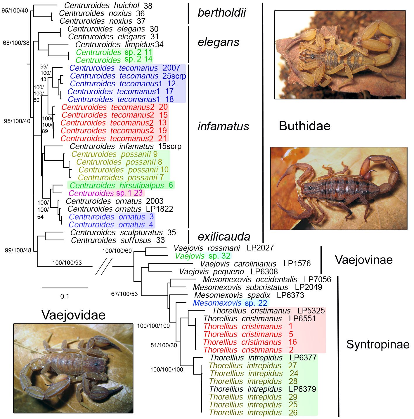
Figure 2. Phylogenetic tree from an analysis of 4 concatenated genetic markers, 3 mitochondrial (12S, 16S, and COI) and 1 nuclear (28S). The topology shows families, subfamilies, and species groups. Numbers beside nodes indicate ultrafast bootstrap/genetic concordance factor/site concordance factor. Colored species represent the 11 species found in our collection within the study area and samples grouping with them distributed inside or outside Colima. Scorpion photos: upper right, Centruroides tecomanus from El Palapo, adult male; middle, Centruroides hirsutipalpus from Sierra de Minatitlán, adult female; lower left, Thorellius intrepidus from El Palapo, adult male.
The Vaejovid clade received full support, except SCF (60%), which included 3 genera: Vaejovis, Mesomexovis, and Thorellius (Fig. 2). The genera occurred in a topology that overall resembles that of González-Santillán and Prendini (2013, 2015); while Vaejovis is a genus within Vaejovinae, Mesomexovis and Thorellius are part of the Syntropinae subfamily. Within Syntropinae, only Thorellius was monophyletic, and T. intrepidus received full support. Additionally, we identified 2 putative new species belonging to the genera Vaejovis and Mesomexovis.
Distributional maps and species geographical ranges. We mined 6,965 records of Mexican scorpions from the InDRE database but retained only 1,000 of the species treated herein. We filtered the records using previously published identified species by specialists and the distribution of the species cited for Colima (González-Santillán & Prendini, 2013, 2018; Lourenço & Sissom, 2000; Ponce-Saavedra et al., 2016; Sissom, 2000).

Figure 3. Map of the west coast of Mexico with georeferenced filtered records from the InDRE database. A, Distribution of Centruroides elegans (circles), records north of Sierra de Manantlán may be misidentifications; B, distribution of Centruroides tecomanus (circles), records in Guerrero (GRO), Guanajuato (GTO), Jalisco (JAL), and Nayarit (NAY) may be misidentifications; Centruroides tecomanus 1 green cross, and Centruroides tecomanus 2 pink crosses. State abbreviations: AUG, Aguascalientes; COL, Colima; MEX, Estado de México; QRO, Querétaro; SLP, San Luis Potosí; ZAC, Zacatecas.

Figure 4. Map of the west coast of Mexico with georeferenced filtered records from the InDRE database and for B additional records from Ponce-Saavedra et al. (2015). A, Distribution of Centruroides infamatus (circles); B, distribution of Centruroides ornatus (circles), our sample in Colima (cross).
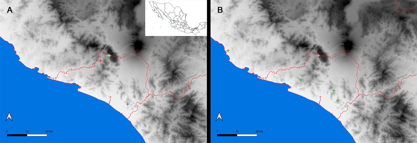
Figure 5. Map of the west coast of Mexico with georeferenced filtered records from the InDRE database. A, Distribution of Centruroides hirsutipalpus (red cross), Centruroides sp. 1 (blue cross), Centruroides sp. 2 (pink cross), and Centruroides possanii (green crosses); B, distribution of Mesomexovis aff. occidentalis sequences in this work and a sample from Chamela Jalisco recorded by González-Santillán (2004), conspecific with our samples in green crosses, Vaejovis sp. (mexicanus group) (pink cross).
The distribution of Centruroides species appears to be restricted by physiographical elements. Centruroides elegans and C. tecomanus are restricted to the coastal lands of Jalisco and Colima, respectively (Fig. 3). The Sierra Madre del Sur appears to be the main barrier to the north of their distribution. The records of these species overlap broadly with a visible gap created by the Sierra de Minatitlán (Fig. 3B) either by subsampling or by an effective geographic barrier.
Centruroides ornatus and C. infamatus, on the other hand, are restricted to the Transmexican Volcanic Belt (TVB) (Fig. 4). While the former species has an entire distribution within this province (Fig. 4B), the latter seems to be distributed in patches, one to the north, along the border of the Chihuahuan desert and the TVB, and the second to the south, between the Balsas Depression and the TVB (Fig. 4A).
Centruroides possanii appears to be a microendemic scorpion species component of the fauna restricted to a massive karstic lone mountain, Cerro Grande (González-Santillán et al., 2019). Two putative undescribed species of Centruroides occupy the extreme east and west of the coastal line of Colima, and C. hirsutipalpus appears restricted to the Sierra Minatitlán (Fig. 5A).
Of the vaejovid species, thus far, the only records for Mesomexovis sp. are in Colima, albeit there is one conspecific record in Chamela, Jalisco (González-Santillán, 2004). The putatively undescribed species of Vaejovis appears restricted to Cerro Grande (Fig. 5B), like Centruroides possanii, potentially another microendemic species. Thorellius intrepidus and T. cristimanus are widely distributed within Colima and across the TVB, the Balsas Depression, and the Sierra Madre del Sur (Fig. 6).
Discussion
Of the 2 families found in Colima, Buthidae comprise 7 species of Centruroides,becoming the most diverse (Table 1, Fig. 2). Our multigene analyses suggest that the previously recorded species C. elegans, C. infamatus, and C. limpidus reported by Ponce-Saavedra et al. (2016) might not be part of the scorpion fauna of Colima, as we demonstrate in the following sections.

Figure 6. Map of the west coast of Mexico with georeferenced filtered records from the InDRE database. A, Distribution of Thorellius intrepidus greensquares, our samples in Colima pink crosses; B, distribution of Thorellius cristimanus greensquares, our samples in Colima pink crosses.
Centruroides elegans and C. limpidus were not found in Colima. Centruroides elegans has an obscure taxonomic history. Firstly, its original description is too general and never indicated a precise type locality, but “Mexico” (Fet & Lowe, 2000). Secondly, although some taxonomic works clarified its former subspecies, the nominal taxon identity of C. elegans remains ambiguous. While Lourenço and Sissom (2000) suggested that this species is distributed in Jalisco, later, González-Santillán (2004) concluded that its distributional limits have never been defined with precision. The 2 exemplars of C. elegans collected in Chamela, Jalisco, grouped with members of the elegans group, sisters to C. limpidus from Iguala, Guerrero, and these in turn, were sister to our 2 exemplars identified as Centruroides new sp. 2 11 and 14 from La Central, in the municipality of Manzanillo (Figs. 2). The distributional data from InDRE of C. elegans is limited right at the northern border of Colima, except for 9 records away from that geographic barrier (Fig. 3A), which we hypothesized as a misidentification due to their position outside the Pacific coastline. Our fieldwork produced no sample conspecific to C. elegans but did produce other genetically distant exemplars. Until denser sampling along the northern border of Colima is conducted, we conclude that C. elegans and by corollary C. limpidus might not be part of the scorpion fauna distributed in Colima as suggested by Ponce-Saavedra and Francke (2013) and Ponce-Saavedra et al. (2016).
Centruroides infamatus may not be part of the Colima scorpion fauna. Centruroides infamatus is another obscure taxon with an ambiguous distributional pattern from published data. Despite its inclusion in phylogenetic analyses (Quijano-Ravel et al., 2019; Towler et al., 2001), its taxonomic circumscription and distribution have never been clarified. Among other problems, the original description indicates “type locality unknown” (Fet & Lowe, 2000). Hoffmann (1932) studied the scorpions from Mexico and realized that the specimens from Michoacán agreed with the original description of the species and proposed that its distribution was expanded to Central Mexico from the Pacific Coast in Sinaloa and Colima to Guanajuato. We included 2 exemplars of C. infamatus, 1 from León, Guanajuato (C. infamatus 15 scrp), and 1 terminal from Tandamangapio municipality, Michoacán (C. infamatus LP1822; Esposito et al., 2018). However, the terminal LP1822 grouped with exemplars of C. ornatus (Fig. 2) and Tandamangapio is approximately 16 km from Sahuayo and Jiquilpan, 2 localities recorded in the redescription of C. ornatus (Ponce-Saavedra et al., 2015).
We plotted 612 records from the InDRE database of C. infamatus to compare the distribution of C. ornatus (Fig. 4A). Although northern Michoacán is almost exclusively occupied by C. ornatus, Jalisco and Michoacán present an overlap with C. infamatus (Fig. 4). Additionally, the InDRE database contains records of C. infamatus from Oaxaca, Puebla, Nayarit, Durango, and Sinaloa (not shown), most likely occupied by other species, implying that most records are misidentifications. The species that morphologically could be confused with C. infamatus in the states of Oaxaca and Puebla are C. baergi, C. nigrovariatus, or C. rodolfoi because the overall base color, body size and carapace pigmentation are similar among the species. The same morphological features are present in specimens from Nayarit and Durango, however, the identity of the populations in these two states have never been studied with a molecular approach and may represent a geographically distinct species.
Nevertheless, recently Ponce-Saavedra et al. (2022) described C. baldazoi for Sinaloa, related morphologically with C. infamatus, potentially a species with which it can be mistaken. Although Ponce-Saavedra and collaborators included C. infamatus in the distribution of Sinaloa and Colima, they failed to indicate precise localities. In summary, the distribution of C. infamatus remains unsolved, attested by the wide distribution reported in the InDRE database. Thus, the infamatus species complex requires comprehensive molecular analyses to delimit its taxonomic circumscription and geographical distribution. On the other hand, our samples of C. ornatus 3 and 4 grouped with C. ornatus LP1822 and with C. ornatus 2003 from Morelia, Michoacán (Esposito & Prendini, 2019), forming a monophyletic group (Fig. 2). Since the samples LP1822 and 2003 lie within the area of C. ornatus proposed by Ponce-Saavedra et al. (2015), we concluded that our exemplars are conspecific with C. ornatus and expanded the distribution southwards, drawing a distributional border in northern Colima (Fig. 4B).
In conclusion, we propose that C. infamatus might not be present in Colima, but further sampling and analyses are needed. Despite the morphological similarity between C. infamatus and C. ornatus, our molecular analysis indicates genetic differences and may present a distinctive distributional pattern yet to be drawn with more samples.
Centruroides tecomanus is a species complex. Due to their morphological similarity with C. limpidus, C. tecomanus was described as C. limpidus tecomanus (Hoffmann, 1932), and the author delimited C. tecomanus distribution to the lowlands of Colima and surmised that its distribution extended to the south along the coastline of Michoacán. But, most importantly, Hoffmann mentioned that on the northern coastline, C. elegans substitutes C. tecomanus. In contrast, the distribution recorded in the InDRE database for C. tecomanus implies that these 2 species present a wide area of sympatry on the coast of Jalisco (Fig. 3).
Ponce-Saavedra et al. (2009) proposed C. tecomanus as a “bona fide species” and assumed its distribution includes the coastline of Michoacán, following Hoffmann (1932). In their molecular and morphological analyses, the authors never included exemplars from Tecomán, Colima, the type locality for the species, assuming that the specimens from Michoacán were conspecific with the populations of Tecomán. Furthermore, Quijano-Ravell et al. (2010) extended the distribution of C. tecomanus to 4 localities in Guerrero and a similar number in Jalisco in a montane area.
The phylogenetic tree presented here substantiates 2 clades of C. tecomanus within the monophyletic infamatus species group (Fig. 2). We hypothesize that these clades may represent potentially distinct sympatric species, emphasizing that our topology obtained full support for these clades with multiple samples. Centruroides tecomanus2 appears to be more common and widely distributed in Colima, whereas C. tecomanus1 is less common, with only 2 localities grouped with Centruroides tecomanus 2007 from Michoacán and from the municipality of Comala, Colima, Centruroides tecomanus (Fig. 3B). Our results suggest that the populations distributed in Michoacán may represent a cryptic, undescribed species; consequently, the exemplars reported in Guerrero (Quijano-Ravell et al., 2010) are unlikely to be conspecific with C. tecomanus. The authors’ discovery of new populations in Jalisco and Guerrero were based entirely on their analyses of morphological characters, precisely the most common way of confusing cryptic species.
Considering that the montane border between Colima and Michoacán is occupied by Centruroides romeroi Quijano-Ravell, de Armas, Francke, Ponce-Saavedra, 2019, it is fair to assume that C. tecomanus1 inhabits coastal ranges following the coastline of Michoacán to the Lázaro Cárdenas delta, where it may be substituted by Centruroides bonito Quijano-Ravell, Teruel, Ponce-Saavedra, 2016 or even other undescribed species. The Balsas River has been proposed to be a geographical barrier for several epigean arachnids, such as Amblypygi and Theraphosidae (Mendoza & Francke, 2017; Schramm et al., 2021) and for small mammals (Ruiz-Vega et al., 2018)
Noteworthy is the locality La Central, right on the border between Colima and Jalisco, a few kilometers southeast of the Marabasco River (Fig. 1A), where we collected 3 putatively different species of Centruroides, the 2 morphotypes of C. tecomanus and Centruroides sp. 2, retrieved within the elegans group (Fig. 2). These findings illustrate the complicated patterns of diversification within this buthid genus in Colima. From a taxonomic perspective, if the identity of C. tecomanus is to be clarified, it is now imperative to analyze molecularly exemplars from Tecomán, Colima, which is the type locality of this species.
Thorellius species exhibit a more restricted distribution in Colima. Thorellius intrepidus and T. cristimanus are widely distributed in several states of the Pacific Lowlands (Fig. 6). However, in a recent revision of the genus, 2 species were described, Thorellius wixarika González-Santillán and Prendini, 2018 and Thorellius tekuani González-Santillán and Prendini, 2018 (Fig. 3 of González-Santillán and Prendini, 2018), that are relevant to these analyses. The former occupies the northwestern territory in Nayarit and Jalisco,whereas the latter inhabits the Balsas Depression of Estado de México, Guerrero, and Michoacán. This observation suggests that the InDRE database contains several misidentifications of both T. intrepidus and T. cristimanus. In fact, the T. wixarika and T. tekuani description was in 2018, and the InDRE database is several years older, hence the complete absence of records. Thus, T. intrepidus inhabits Aguascalientes, Colima, Guanajuato, Jalisco, and Michoacán (Fig. 6A); and T. cristimanus, Colima and Jalisco (González-Santillán & Prendini, 2018) (Fig. 6B). From an ecological point of view, we noticed that the InDRE database only has records with elevations below 700 m, implying that these species prefer tropical to subtropical climates in Colima.
González-Santillán (2004) reported Mesomexovis aff. occidentalis as a putative new species for the Biological Station Chamela, Jalisco. Furthermore, González-Santillán and Prendini (2015) conducted a phylogenetic analysis using morphology and mitochondrial and nuclear DNA, resulting in a topology that suggested that this species was not conspecific to Mesomexovis occidentalis, as Williams (1986)identified it. López-Granados (2019) found further morphological evidence to separate this species, but the evidence was never published. The importance of that work is that, for the first time, exemplars of Mesomexovis from Colima that were conspecific with our samples were included in a phylogenetic analysis. Once more, we demonstrate that Mesomexovis sp. 22 is not conspecific with M. occidentalis using molecular evidence, and it requires a formal separation and description (Fig. 2). Unlike Thorellius species in Colima, Mesomexovis is a widespread species inhabiting tropical to montane habitats with a wider range of elevation (Fig. 5B).
The mexicanus group was recently revisited in a monograph with the delimitation of other species groups and the description of 5 new species (Contreras-Félix & Francke, 2019). The paucity of sequences for the mexicanus group in the NCBI database only permitted retrieval of loci for Vaejovis rossmani LP 2027, a species inhabiting the Sierra Madre Oriental in the states of Tamaulipas and Nuevo León and treated in the Contreras-Félix and Francke (2019) monograph. Our analysis retrieved Vaejovis sp. 32 and Vaejovis rossmani LP 2027 together, which suggests membership of the mexicanus group of Vaejovis. Furthermore, Vaejovis sp. 32also matches the morphological diagnosis presented in Contreras-Felix and Francke (2019). Contreras-Félix et al. (2023) recorded Vaejovis santibagnezi Contreras-Felix and Francke, 2019 in Cerro Grande, where we collected our samples (Fig. 5B). However, the authors failed to present morphological evidence to justify this conclusion. We compared our specimens with the geographically closest V. monticola deposited in the CNAN and with V. santibagnezi and found significant morphological differences. Currently, we are preparing a contribution where we propose the description of a new species. Following this idea, we are inclined to think that, like C. possanii, Vaejovis sp. 32 is also microendemic because of its limitation to disperse throughout tropical valleys from the Cerro Grande massif to other mountain ranges. Finally, we submit that such an evident geographical barrier may apply to several epigean, non-volant arthropods such as the scorpions.
Finally, 2 species absent in our fieldwork are Konetontli ilitchi González-Santillán and Prendini 2015 and Vaejovis janssi Williams, 1980. The latter is endemic to the Socorro Island, part of the Revillagigedo Archipelago (Williams, 1980), and K. ilitchi has been found only inside a cave in the vicinity of Coquimatlán, Colima (González-Santillán & Prendini, 2015). These 2 features in the distribution and biology of the species hindered the possibility of collecting and studying them. Future fieldwork may illuminate the taxonomy and distribution of these elusive species. Finally, Vaejovis monticola, another high elevation dweller of the mexicanus species group (Contreras-Felix & Francke 2019) was absent in our collecting trips. Although its type locality cited by Contreras-Felix and Francke (2019) indicates: “Jalisco, northern side of Nevado de Colima” we submit that it may not be on the southern side in Colima, but extensive fieldwork is needed to confirm this hypothesis.
Biogeographical and ecological considerations
There is strong evidence that the ancestors of the North American Centruroides originated in Gondwana and have dispersed to and diversified in that territory via land bridges, vicariance, and rafting over the Atlantic Ocean, over 50 to 20 Mya (Esposito & Prendini, 2019). However, the movement of this genus towards boreal latitudes within North America is not well understood. Although one could suppose that the colonization of such territories appears to be in pulses at different periods due to the overlap in the distribution of the elegans and infamatus species groups, it is beyond the scope of our study to establish a coherent explanation; besides, our data are incomplete to that end. One startling discovery is that the Colima scorpiofauna comprises 7 distinctive, at least genetically, species of Centruroides (Fig. 2). What biotic, abiotic, or ecological factors produce such species diversity? Is it a combination of all these factors? Is it a case of sympatric speciation? Morphologically, it is sometimes difficult to distinguish some of these species. For instance, the 3 species found in La Central were identified initially as C. tecomanus because they exhibit no morphological variation, at least in traditional characters shown in identification keys (Ponce-Saavedra et al., 2016). It is fundamental to conduct morphological studies with this scorpion community to obtain independent information to precisely delimit these species. Unlike other scorpion groups, Centruroides exhibit conservative morphology. For instance, if we compared Centruroides species to species of the Syntropinae subfamily, we find that syntropines are diverse in ecomorphotypic adaptations that promoted morphological diversification (González-Santillán & Prendini, 2013), while in Centruroides, the persistent errant lifestyle maintains morphology without significant variation. It is astonishing to observe, for instance, C. tecomanus living at sea level in tropical deciduous forests and compare it to C. possanii inhabiting pine-oak forests above 2,000 m elevation; as though, the same “Centruroides bauplan” can survive diametrically different environments following a persistent lifestyle. This final assertion leads us to think that the adaptative changes are in the physiology rather than in the morphology of Centruroides.
Thorellius and Mesomexovis (Syntropinae) are substrate-specialists, since the body plan, more robust and armed with setae and spinules on the legs, allow these species to scrape and dig galleries on clayey, fine-grained substrates (González-Santillán & Prendini, 2013, 2018). Such adaptations come with a drawback because the kind of soil restricts the presence of these scorpions; for instance, rocky or shallow soils represent unhospitable habitats for these species. Like other species in the mexicanus group, Vaejovis sp. 32 and Vaejovis monticola Sissom, 1989 are inhabitants of montane habitats within the intricate topography of Colima.
In summary, the scorpion assemblage distributed in Colima includes errant species such as Centruroides without exaggerated adaptations; pelophilous/lapidicolous species such as Thorellius and Mesomexovis, powerful diggers, commonly found underneath rocks or other debris; and scorpions that can be found inside the leaf litter or under nooks of rocks or trees, such as Vaejovis sp. However, it is enigmatic why the Diplocentridae family, well-represented in Mexico, has not been found in Colima. Only in Colima, out of the 3 relatively small states in Mexico, the other 2 being Morelos (Santibáñez-López et al., 2011) and Aguascalientes (Chávez-Samayoa et al., 2022), where similar scorpiofaunistic surveys have been conducted, the genus Diplocentrus is absent. From a biogeographical point of view, if this family is absent in Colima, it is not trivial and requires further investigation.
As a final remark, we hope we have accomplished our aim of urging arachnologists to examine the benefits of local inventories and the potential use of barcodes at the forefront of discovering and documenting local arachnid diversity.
Medical and pharmacological relevance of some scorpions of Colima
From a medical point of view, it is of utmost importance to identify the species of scorpions in an area and to be able to distinguish hazardous from harmless species. Colima is one of the states with the highest incidence rates of mortality and morbidity caused by intoxication by scorpion sting (ISS) (Chowell et al., 2006; González-Santillán & Possani, 2018). By the 1940s, Colima was at the forefront of ISS and deaths in Mexico. However, with the introduction of a safe and effective antivenom in the 1970s, mortality has diminished, although morbidity is still high (González-Santillán & Possani, 2018).
Due to the medical relevance of scorpionism in Mexico, the venom of some buthid scorpions distributed in Colima has been studied extensively (Table 6). We know that mammalian sodium scorpion toxins (NaScTx) are the chief and sometimes most abundant compound responsible for the toxicity of scorpion venom, although potassium, chlorine, and calcium-gated channels, among others, are also affected by toxic peptides (Cid-Uribe et al., 2019; González-Santillán & Possani 2018). Until now, C. hirsutipalpus, C. ornatus, C. possanii, and C. tecomanus have been studied with a proteomic or transcriptomic approach, demonstrating that these venoms are powerful enough to decimate humans (García-Guerrero et al., 2020; García-Villalvazo et al., 2023, Valdez-Velázquez et al., 2016, 2018). Centruroides tecomanus venom contains at least 13 mammalian toxic compounds (Valdez-Velázquez et al., 2016), of which Ct1a is the main mammalian sodium scorpion toxin component, with a molecular weight of 7,591 Da (Martin et al., 1988). The proteomic analysis of C. ornatus toxic components identified 3 major mammalian NaScTx, CO1, CO2, and CO3, with molecular weights of 7,561.2, 7,614.3, and 7,774.9 Da, respectively (García-Guerrero et al., 2020). On the other hand, the published mass fingerprint of C. hirsutipalpus venom has 4 compounds with similar molecular weight to C. tecomanus peptides, suggesting that these species may have similar or identical NaScTx (Valdez-Velázquez et al., 2018). One of the shared compounds found in C. hirsutipalpus corresponds to the molecular weight of Ct1a (Valdez-Velázquez et al., 2013), which means that Ct1a could be responsible for, or at least contribute to, the high toxicity of this species. Although the molecular components with a weight corresponding to the toxic peptides CO1, CO2, and CO3 are not present in C. hirsutipalpus venom, the mass fingerprint of C. tecomanus reported a peptide with similar molecular weight to CO2 toxin present in C. ornatus (Valdez-Velázquez et al., 2013). Our phylogenetic results show that these species belong to the infamatus group, and it is notable that the molecular weight among some toxins is similar. This observation opens the possibility that the toxin diversity of the mammalian NaScTx may have been inherited from a common ancestor. We realize, however, the need for a more in-depth study to unveil the relationship among these toxic peptides to test such a hypothesis. In contrast, a C. possanii crude venom proteomic study resulted in the identification of 18 NaScTx, of which, CpoNatBet09 was identical to Cll2b and Cii1 from C. limpidus and C. infamatus, respectively (Valdez-Velázquez et al., 2013). This example allows us to present the counterpart of the previous one. Centruroides limpidus in our topology grouped with members of the elegans group and C. possanii within the infamatus group (Fig. 2). We can conclude that the exact sequence match between CpoNatBet09 and Cll2b is most likely due to a selective force that produced convergent evolution. Alternatively, this is a deeper inheritance within the ancestors of the infamatus and elegans group.
The comparisons and hypotheses about venom similarities and species assume that all scorpions used to conduct the experiments to obtain the crude venom were correctly identified. However, the discovery of putative species of Centruroides might question some of these results, particularly those of C. tecomanus. The first author has been collaborating to identify most samples of species used in some of the recently published investigation on venom research (Cid-Uribe et al., 2019; García-Guerrero et al., 2020; Romero-Gutiérrez et al., 2017, Valdez-Velázquez et al., 2018, among others). And in some cases, voucher specimens have been deposited in the CNAN, therefore the taxonomic identity for C. hirsutipalpus, C. ornatus, C. possanii can be readily corroborated.
Table 6
Scorpion species with reported LD50 tested on mice at μg/20g mouse weight scale with the named, most abundant, and likely responsible for high toxicity sodium toxins found in the scorpion species of Colima.
| Species | LD50 | NaScTx | Autor |
| Centruroides hirsutipalpus Ponce-Saavedra and Francke, 2009 | 11.7 ± 1.9 | 26 β-NaTx and 5 α-NaTx (proteome) 71 β-NaTx and 16 α-NaTx (transcriptome) | Valdez-Velázquez et al. (2021) |
| Centruroides ornatus Pocock, 1902 | 13.3 ± 1.7 | Beta toxins: Co1, Co2, Co3, Co52 | García-Guerrrero et al. (2020) |
| Centruroides possanii González-Santillán, Galán-Sánchez, Valdez-Velázquez, 2019 | 13.18 ± 0.7 | CpoNatBet09, CpoNatBet14, CpoNatBet35 (Proteome and transcriptome) | García-Villalvazo et al. (2023) |
| Centruroides tecomanus Hoffmann, 1932 | 10.2 ± 0.3 | Beta toxin Ct1a, Ct7, Ct16, Ct17, Ct28, Ct25, Ct6, Ct13, neutoroxin II.22.5 | Valdez-Velázquez et al. (2013, 2016), Ramírez et al. (1988) |
| Thorellius cristimanus Pocock, 1902 | N/A | 10 β-NaTx and 3 α-NaTx (transcriptome) | Romero-Gutiérrez et al. (2017) |
Because vaejovid scorpions exhibit lower toxin potency, proteomic studies are uncommon. However, the study of the crude venom of Thorellius cristimanus under a transcriptomic and proteomic approachidentified160 potential venom peptides (Romero-Gutiérrez et al., 2017). The authors found a great diversity of channel toxins targeting potassium and calcium ion-channels, numerous enzymes, and NDBP. Nevertheless, none of these toxins appear to affect mammals to endanger their life. Noteworthy are the NDBP compounds with antimicrobial activity (Almaaytah et al., 2014), which potentially may be a source for developing novel commercial antibiotics. More recently, Ibarra-Vega et al. (2023) reported finding the neurotransmitter serotonin and 2 derived or intermediate indoles of serotonin: N-methylserotonin, and bufotenidine. Although serotonin has been reported in other scorpions and the sea snail genus Conus, the other indoles represent the first report in scorpions. The authors proposed that the 3 components are involved in defense and probably prey submission because they produce extreme pain in the victim. Furthermore, N-methylserotonin and bufotenidine showed a similar affinity for serotonin cellular receptors, implying a role in the effect of this neurotransmitter, and thus, it showed promising medical applications.
Integrating taxonomic, distributional, and in our case venom diversity within local scorpion faunas is an interdisciplinary topic uncommon in the literature (Brito & Borges, 2015; Cao et al., 2014), although this exercise has been done in Mexico before (Santibáñez-López et al., 2015). This multidisciplinary work took advantage of a reciprocal illumination exercise. This short synthesis of the diversity of venoms of scorpion of Colima revealed the potential of toxins to be part of the evidence to identify and delimit species (Schaffrath et al., 2018). Moreover, the synthesis provided a glance of the evolution of venoms not only for the medically prominent species of Centruroides but also for vaejovid scorpion species. From the experimental discipline, we learned that it is paramount to maintain vouchers after biochemical or physiological experiments to track down the original material and keep up with the dynamics of taxonomy, a tool requiring empirical information to permit the identification of species to validate past, present, and future discoveries in other biological disciplines.
Acknowledgments
We thank the University of Colima students and Josué López Granados (Facultad de Ciencias, UNAM) for their assistance in collecting scorpions throughout the state of Colima. JICU thanks Conahcyt for granting a postdoctoral scholarship (512560). Collection permits granted by Semarnat included SGPA/DGVS/12063/15, SGPA/DGVS/02139/2022, and FAUT-0305. Finally, we are grateful to the Associate Editor and two reviewers for improving an early version of the manuscript, particularly to Andrés Ojanguren-Afilastro for his critical reading.
References
Almaaytah, A., & Albalas, Q. (2014). Scorpion venom peptides with no disulfide bridges: a review. Peptides, 51, 35−45. https://doi.org/10.1016/j.peptides.2013.10.021
Baldazo-Monsivaiz, J. G., Ponce-Saavedra, J., & Flores-Moreno, M. (2012). Los alacranes (Arachnida: Scorpionida) de importancia médica del estado de Guerrero, México. Dugesiana, 19, 143−150.
Baldazo-Monsivaiz, J. G., Teruel, R., Cortés-Guzmán, A. J., & Canché-Aguilar, I. (2017). Los escorpiones (Arachnida: Scorpiones) del municipio de Chilpancingo de los Bravo, estado de Guerrero, México Entomología Mexicana, 4, 21−27.
Baldazo-Monsivaiz, J. G., Teruel, R., Cortés-Guzmán, A. J., Sánchez-Arriaga, J., López-Flores, M., Reyes-Castelán, A. et al. (2016). Los escorpiones (Arachnida: Scorpiones) del municipio de Taxco de Alarcón, del estado de Guerrero, México. Entomología Mexicana, 3, 75−80.
Bolaños, L. M., Rosenblueth, M., de Lara, A. M., Migueles-Lozano, A., Gil-Aguillón, C., Mateo-Estrada, V. et al. (2019). Cophylogenetic analysis suggests cospeciation between the Scorpion Mycoplasma Clade symbionts and their hosts. Plos One, 14, e0209588 https://doi.org/10.1371/journal.pone.0209588
Brito, G., & Borges, A. (2015). A checklist of the scorpions of Ecuador (Arachnida: Scorpiones), with notes on the distribution and medical significance of some species. Journal of Venomous Animals and Toxins Including Tropical Diseases, 21, 1–23. https://doi.org/10.1186%2Fs40409-015-0023-x
Cao, Z., Di, Z., Wu, Y., & Li, W. (2014). Overview of scorpion species from China and their toxins. Toxins, 6, 796–815. https://doi.org/10.3390/toxins6030796
Cid-Uribe, J. I., Meneses E. P., Batista, C. V. F., Ortiz, E., & Possani, L. D. (2019). Dissecting toxicity: The venom gland transcriptome and the venom proteome of the highly venomous scorpion Centruroides limpidus (Karsch, 1879). Toxins, 247, 1−21. https://doi.org/10.3390/toxins11050247
Contreras-Félix, G. A., & Francke, O. F. (2019). Taxonomic revision of the “mexicanus” group of the genus Vaejovis C. L. Koch, 1836 (Scorpiones: Vaejovidae). Zootaxa, 4596, 1−100. https://doi.org/10.11646/zootaxa.4596.1.1
Contreras-Félix, G. A., del Pozo, O. G., & Navarrete-Heredia, J. L. (2023). A new species of Vaejovis from the mountains of west Mexico (Scorpiones: Vaejovidae). Dugesiana, 30, 229−245. https://doi.org/10.32870/dugesiana.v30i2.7306
Chávez-Samayoa, F., Díaz-Plascencia, J. E., & González-Santillán, E. (2022). Two new species of Vaejovis (Scorpiones: Vaejovidae) belonging to the mexicanus group from Aguascalientes, Mexico, with comments on the homology and function of the hemispermatophore. Zoologischer Anzeiger, 298, 148–169. https://doi.org/10.
1016/j.jcz.2022.04.005
Chowell, G., Díaz-Dueñas, P., Bustos-Saldaña, R., Alemán-Mireles, A., & Fet, V. (2006). Epidemiological and clinical characteristics of scorpionism in Colima, Mexico (2000-2001). Toxicon, 47, 753–758. https://doi.org/10.1016/j.toxicon.2006.02.004
Esposito, L. A., & Prendini, L. (2019). Island ancestors and New World biogeography: a case study from the scorpions (Buthidae: Centruroidinae). Scientific Reports, 9, 3500. https://doi.org/10.1038/s41598-018-33754-8
Fet, V., Graham, M. R., Blagoev, G., Karataş, A., & Karataş, A. (2016). DNA barcoding indicates hidden diversity of Euscorpius (Scorpiones: Euscorpiidae) in Turkey. Euscorpius, 216, 1–13.
Fet, V., Graham, M. R., Webber, M. M., & Blagoev, G. (2014). Two new species of Euscorpius (Scorpiones: Euscorpiidae) from Bulgaria, Serbia, and Greece. Zootaxa, 3894, 83–105. https://doi.org/10.11646/zootaxa.3894.1.7
Fet, V., & Lowe G. (2000). Family Buthidae C. L: Koch, 1837. In V. Fet, W. D. Sissom, G. Lowe, & M. E. Braunwalder (Eds.), Catalog of the scorpions of the World (1758–1998) (pp. 54–286). New York: New York Entomological Society.
Folmer, O., Black, M., Hoeh, W., Lutz, R., & Vrijenhoek, R. (1994). DNA primers for amplification of mitochondrial cytochrome c oxidase subunit I from diverse metazoan invertebrates. Molecular Marine Biology and Biotechnology, 3, 294–299.
García-Guerrero, I. A., Cárcamo-Noriega, E., Gómez-Lagunas, F., González-Santillán, E., Zamudio, F. Z., Gurrola, G. B. et al. (2020). Biochemical characterization of the venom from the Mexican scorpion Centruroides ornatus, a dangerous species to humans. Toxicon, 15, 27–38. https://doi.org/10.1016/j.toxicon.2019.11.004
García-Villalvazo, P. E., Jiménez-Vargas, J. M., Lino-López, G. J., Meneses, E. P., Bermúdez-Guzmán, M. J., Barajas-Saucedo, C. E. et al. (2023). Unveiling the protein components of the secretory-venom gland and venom of the scorpion Centruroides possanii (Buthidae) through omic technologies. Toxins, 15, 1–20. https://doi.org/10.3390/toxins15080498
Goodman, A. M., Prendini, L., & Esposito, L. A. (2021). Systematics of the arboreal Neotropical ‘thorellii’ clade of Centruroides bark scorpions (Buthidae) and the efficacy of mini-barcodes for museum specimens. Diversity, 13, 441. https://doi.org/10.3390/d13090441
Goodman, A. M., Prendini, L., Francke, O. F., & Esposito, L. A. (2021). Systematic revision of the arboreal neotropical “thorellii” clade of Centruroides Marx, 1890, bark scorpions (Buthidae C. L. Koch, 1837) with descriptions of six new species. Bulletin of the American Museum of Natural History, 452, 1–92.
González-Santillán, E. (2004). Diversidad, taxonomía y hábitat de alacranes. In A. N. García, & R. Ayala (Eds.), Artrópodos de Chamela (pp. 25–35). México D.F.: Instituto de Biología, Universidad Nacional Autónoma de México.
González-Santillán, E., Galán-Sánchez, M. A., & Valdez-Velázquez, L. L. (2019). A new species of Centruroides (Scorpiones, Buthidae) from Colima, Mexico. Comptes Rendus Biologies, 342, 9–10. https://doi.org/10.1016/j.crvi.2019.10.002
González-Santillán, E., & Possani, L. D. (2018). North American scorpion species of public health importance with a reappraisal of historical epidemiology. Acta Tropica, 187, 264–274. https://doi.org/10.1016/j.actatropica.2018.08.002
González-Santillán, E., & Prendini, L. (2013). Redefinition and generic revision of the North American vaejovid scorpion subfamily Syntropinae Kraepelin, 1905, with descriptions of six new genera. Bulletin of the American Museum of Natural History, 382, 1–71.
González-Santillán, E., & Prendini, L. (2015). Phylogeny of the North American vaejovid scorpion subfamily Syntropinae Kraepelin, 1905, based on morphology, mitochondrial and nuclear DNA. Cladistics, 31, 341–405. https://doi.org/10.1111/cla.12091
González-Santillán, E., & Prendini, L. (2018). Systematic revision of the North American Syntropine Vaejovid scorpion genera Balsateres, Kuarapu, and Thorellius, with descriptions of three new species. Bulletin of the American Museum of Natural History, 420, 1–81. https://doi.org/10.1206/0003-0090-420.1.1
Hoang, D. T., Chernomor, O., Haeseler, A. von, Minh, B. Q., & Vinh, L. S. (2018) UFBoot2: Improving the ultrafast bootstrap approximation. Molecular Biology and Evolution, 35, 518–522. https://doi.org/10.1093/molbev/msx281
Hoffmann, C. C. (1932). Monografías para la entomología médica de México. Monografía Núm. 2. Los scorpiones de Mexico. Segunda parte, Buthidae. Anales del Instituto de Biología, Universidad Nacional Autónoma de México, 3, 243–361.
Huerta-Jiménez, H. (2018). Actualización de la Colección de Artrópodos con importancia médica (CAIM), Laboratorio de Entomología, InDRE. Version 1.5. Comisión Nacional para el Conocimiento y uso de la Biodiversidad.
Ibarra-Vega, R., Jiménez-Vargas, J. M., Pineda-Contreras, A., Martínez-Martínez, F. J., Barajas-Saucedo, C. E., García-Ortega, H. et al. (2023). Indolealkylamines in the venom of the scorpion Thorellius intrepidus. Toxicon, 233, 107232. https://doi.org/10.1016/j.toxicon.2023.107232
Jarvis, A., Reuter, H. I., Nelson, A. & Guevara, E. (2008). Hole-filled seamless SRTM data V4, International Centre for Tropical Agriculture (CIAT), available from http://srtm.csi.cgiar.org
Kalyaanamoorthy, S., Minh, B. Q., Wong, T. K. F., Haeseler, A. von, & Jermiin, L. S. (2017). ModelFinder: fast model selection for accurate phylogenetic estimates. Nature Methods, 14, 587–589. https://doi.org/10.1038/nmeth.4285
Katoh, K., Rozewicki, J., & Yamada, K. D. (2019). MAFFT online service: multiple sequence alignment, interactive sequence choice and visualization, Briefings in Bioinformatics, 20, 1160–1166. https://doi.org/10.1093/bib/bbx108
Kocher, T. D., Thomas, W. K., Meyer, A., Edwards, S. V., Paabo, S., Villablanca, F. X. et al. (1989). Dynamics of mitochondrial DNA evolution in animals: amplification and sequencing with conserved primers. Proceedings of the National Academy of Sciences, 86, 6196–6200. https://doi.org/10.1073%2Fpnas.86.16.6196
Kuraku, S., Zmasek, C. M., Nishimura, O., & Katoh, K. (2013). aLeaves facilitates on-demand exploration of metazoan gene family trees on MAFFT sequence alignment server with enhanced interactivity, Nucleic Acids Research, 41, W22–W28. https://doi.org/10.1093/nar/gkt389
López-Granados, J. (2019). Análisis filogenético del complejo de especies occidentalis del género Mesomexovis González-Santillán y Prendini, 2013 (Scorpiones: Vaejovidae) basado en evidencia morfológica (Tesis). Facultad de Ciencias, Universidad Nacional Autónoma de México. CDMX.
Lourenço, W. R., & Sissom, W. D. (2000). Scorpiones. In B. J. Llorente, E. González, & N. Papavero (Eds.), Biodiversidad, taxonomía y biogeografía de artrópodos de México: hacia una síntesis de su conocimiento (pp. 115–135). Ciudad de México: Universidad Nacional Autónoma de México.
Maddison, W. P., & Maddison, D. R. (2023). Mesquite: a modular system for evolutionary analysis. Version 3.81. http://www.mesquiteproject.org
Martin, B. M., Carbone, E., Yatani, A., Brown, A. M., Ramírez, A. N., Gurrola, G. B. et al. (1998). Amino acid sequence and physiological characterization of toxins from the venom of the scorpion Centruroides limpidus tecomanus Hoffmann. Toxicon, 26, 785–94. https://doi.org/10.1016/0041-0101(88)90319-4
Mendoza, J., & Francke, O. (2017). Systematic revision of Brachypelma red-kneed tarantulas (Araneae: Theraphosidae), and the use of DNA barcodes to assist in the identification and conservation of CITES-listed species. Invertebrate Systematics, 31, 157–179. https://doi.org/10.1071/IS16023
Minh, B. Q., Hahn, M. W., & Lanfear, R. (2020). New methods to calculate concordance factors for phylogenomic datasets. Molecular Biology and Evolution, 37, 2727–2733. https://doi.org/10.1093/molbev/msaa106
Morrone, J. (2019). Regionalización biogeográfica y evolución biótica de México: encrucijada de la biodiversidad del Nuevo Mundo. Revista Mexicana de Biodiversidad, 90, e902980. https://doi.org/10.22201/ib.20078706e.2019.90.2980
Morrone, J., Escalante, T., & Rodríguez-Tapia, G. (2017). Mexican biogeographic provinces: map and shapefiles. Zootaxa, 4277, 277–279. https://doi.org/10.11646/zootaxa.4277.2.8
Nguyen, L. T., Schmidt, H. A., Haeseler, A. von, & Minh, B. Q. (2015). IQ-TREE: a fast and effective stochastic algorithm for estimating maximum likelihood phylogenies. Molecular Biology and Evolution, 32, 268–274. https://doi.org/10.1093/molbev/msu300
Nunn, G. B., Theisen, B. F., Chirstensen, B., & Arctander, P. (1996). Simplicity-correlated size growth of the nuclear 28S ribosomal RNA D3 expansion segment in the crustacean order Isopoda. Journal of Molecular Evolution, 42, 211–223. https://doi.org/10.1007/bf02198847
Podnar, M., Grbac, I., Tvrtković, N., Hörweg, C., & Haring, E. (2021). Hidden diversity, ancient divergences, and tentative Pleistocene microrefugia of European scorpions (Euscorpiidae: Euscorpiinae) in the eastern Adriatic region. Journal of Zoological Systematics and Evolutionary Research, 59, 1824–1849. https://doi.org/10.1111/jzs.12562
Ponce-Saavedra, J., & Francke, O. F. (2013). Clave para la identificación de especies de alacranes del género Centruroides Marx 1890 (Scorpiones: Buthidae) en el Centro Occidente de México. Biológicas, 15, 52–62.
Ponce-Saavedra, J. y Francke, O. F. (2019). Una especie nueva de alacrán del género Centruroides (Scorpiones: Buthidae) del noroeste de México. Revista Mexicana de Biodiversidad,
90, e902660. https://doi.org/10.22201/ib.20078706e.2019.
90.2660
Ponce-Saavedra, J., Francke, O. F., Cano-Camacho, H., & Hernández-Calderón, E. (2009). Evidencias morfológicas y moleculares que validan como especie a Centruroides tecomanus (Scorpiones, Buthidae). Revista Mexicana de Biodiversidad, 80, 71–84. https://doi.org/10.22201/ib.20078706e.2009.001.585
Ponce-Saavedra, J., Francke, O. F., Quijano-Ravell, A. F., & Santillán, R. C. (2016). Alacranes (Arachnida: Scorpiones) de importancia para la salud pública de México. Folia Entomológica Mexicana, 2, 45–70.
Ponce-Saavedra, J., Jiménez, M. L., Quijano-Ravell, A. F., Vargas-Sandoval, M., Chamé-Vázquez, D., Palacios-Cardiel, C. et al. (2023). The Fauna of Arachnids in the Anthropocene of Mexico, Chapter 2(pp. 18–39) In R. W. Jones, C. P. Ornelas-García, R. Pineda-López, & F. Álvarez (Eds.), Mexican fauna in the Anthropocene. Cham, Switzerland: Springer. https://doi.org/10.1007/978-3-031-17277-9
Ponce-Saavedra, J., Linares-Guillén, J. W., & Quijano-Ravell, A. F. (2022). Una nueva especie de alacrán del género Centruroides Marx (Scorpiones: Buthidae) de la costa Noroeste de México. Acta Zoológica Mexicana (nueva serie), 38, 1–24. https://doi.org/10.21829/azm.2022.3812517
Ponce-Saavedra, J., Quijano-Ravell, A. F., Teruel, R., & Francke, O. F. (2015). Redescription of Centruroides ornatus Pocock, 1902 (Scorpiones: Buthidae), a montane scorpion from Central Mexico. Revista Ibérica de Aracnología, 27, 81–89.
Prendini, L., Weygoldt, P., & Wheeler, W. C. (2005). Systematics of the Damon variegatus group of African whip spiders (Chelicerata: Amblypygi): evidence from behaviour, morphology and DNA. Organisms Diversity & Evolution, 5, 203–236. https://doi.org/10.1016/j.ode.2004.12.004
Quijano-Ravell, A. F., De Armas, L. F., Francke, O. F., & Ponce-Saavedra, J. (2019). A new species of the genus Centruroides Marx (Scorpiones, Buthidae) from western Michoacán state, México using molecular and morphological evidence. Zookeys, 859, 31–48. https://doi.org/10.3897/zookeys.859.33069
Quijano-Ravell, A. F., Ponce-Saavedra, J., Francke, O. F., & Villaseñor-Ramos. M. A. (2010). Nuevos registros y distribución actualizada de Centruroides tecomanus Hoffmann, 1931 (Scorpiones: Buthidae). Ciencia Nicolaita, 52, 179–189.
QGIS.org. (2021). QGIS Geographic Information System. Open-Source Geospatial Foundation Project. http://qgis.org
Ramírez-Ruiz, J. J., & Bretón-González, M. (2016). Fisiografía y geología. In La Biodiversidad en Colima. Estudio de estado (Eds.) (pp. 25–31). México D.F.: Conabio.
Romero-Gutiérrez, T., Peguero-Sánchez, E., Cevallos, M. A., Batista, C. V. F., Ortiz, E., & Possani L. D. (2017). A deeper examination of Thorellius atrox scorpion venom components with omics technologies. Toxins, 9, 399. https://doi.org/10.3390/toxins9120399
Ruiz-Vega, M. L., Hernández-Canchola, G., & León-Paniagua, L. (2018). Molecular systematics and phylogeography of the endemic Osgood’s deermouse Osgoodomys banderanus (Rodentia: Cricetidae) in the lowlands of western Mexico. Molecular Phylogenetics and Evolution, 127, 867–877. https://doi.org/10.1016/j.ympev.2018.06.034
Santibáñez-López, C. E., Francke, O. F., & Córdova-Athanasiadis, M. (2011). The genus Diplocentrus Peters (Scorpiones: Diplocentridae) in Morelos, Mexico. Revista Ibérica de Aracnología, 19, 3–3.
Santibáñez-López, C. E., Francke, O. F., & Prendini, L. (2014). Phylogeny of the North American scorpion genus Diplocentrus Peters, 1861 (Scorpiones: Diplocentridae) based on morphology, nuclear and mitochondrial DNA. Arthropod Systematics & Phylogeny, 72, 257–279. https://doi.org/10.3897/asp.72.e31789
Santibáñez-López, C., Francke, O., Ureta, C., & Possani, L. (2015). Scorpions from Mexico: from species diversity to venom complexity. Toxins, 8, 1–18. https://doi.org/10.3390/toxins8010002
Schaffrath, S., & Predel, R. (2014). A simple protocol for venom peptide barcoding in scorpions. EuPA Open Proteomics, 3, 239–245. https://doi.org/10.1016/j.euprot.2014.02.017
Schramm, F. D., Valdez-Mondragón, A., & Prendini, L. (2021). Volcanism and palaeoclimate change drive diversification of the world’s largest whip spider (Amblypygi). Molecular Ecology, 30, 2872–2890. https://doi.org/10.1111/mec.15924
Simon, C., Frati, F., Beckenbach, A., Crespi, B., Liu, H., & Flook, P. K. (1994). Evolution, weighting, and phylogenetic utility of mitochondrial gene sequences and a compilation of conserved polymerase chain reaction primers. Annals of the Entomological Society of America, 87, 651–700. https://doi.org/10.1093/aesa/87.6.651
Sissom, W. D. (2000). Family Vaejovidae Thorell, 1876. In V. Fet, W. D. Sissom, G. Lowe, & M. E. Braunwalder (Eds.), Catalog of the scorpions of the World (1758–1998) (pp. 503–553). New York: New York Entomological Society.
Towler, W. I. I., Ponce-Saavedra, J., Gantenbein, B., & Fet, V. (2001). Mitochondrial DNA reveals a divergent phylogeny in tropical Centruroides (Scorpiones: Buthidae) from Mexico. Biogeographica, 77, 157–172.
Valdez-Velázquez, L. L., Olamendi-Portugal, T., Restano-Cassulini, R., Zamudio, F. Z., & Possani, L. D. (2018). Mass fingerprinting and electrophysiological analysis of the venom from the scorpion Centruroides hirsutipalpus (Scorpiones: Buthidae). Journal of Venom Animal Toxins Including Tropical Diseases, 24, 17. https://doi.org/10.1186/s40409-018-0154-y
Valdez-Velázquez, L. L., Quintero-Hernández, V., Romero-Gutiérrez, M. T., Coronas, F. I., & Possani, L. D. (2013). Mass fingerprinting of the venom and transcriptome of venom gland of scorpion Centruroides tecomanus. Plos One, 8, e66486. https://doi.org/10.1371/journal.pone.0066486
Valdez-Velázquez L. L., Romero-Gutiérrez M. T., Delgado-Enciso, I., Dobrovinskaya, O., Melnikov, V., Quintero-Hernández, V. et al. (2016). Comprehensive analysis of venom from the scorpion Centruroides tecomanus reveals compounds with antimicrobial, cytotoxic, and insecticidal activities. Toxicon, 118, 95-103. https://doi.org/10.1016/j.toxicon.2016.04.046
Williams, S. C. (1980). Scorpions of Baja California, Mexico and adjacent islands. Occasional Papers of the California Academy of Sciences, 135, 1–127.
Williams, S. C. (1986). A new species of Vaejovis from Jalisco, Mexico (Scorpiones: Vaejovidae). Pan-Pacific Entomologist, 62, 355–358.

Five new species of Pseudachorutes (Collembola: Neanuridae) from Mexico
José G. Palacios-Vargas a, Erika Rivero-Sánchez a, Yan Gao b, Margarita Ojeda a, *
a Universidad Nacional Autónoma de México, Facultad de Ciencias, Departamento de Ecología y Recursos Naturales, Laboratorio de Ecología y Sistemática de Microartrópodos, Circuito Exterior s/n, Ciudad Universitaria, Coyoacán, 04510 Mexico City, Mexico
b China Shanghai Natural History Museum, Shanghai Science & Technology Museum, Shanhaiguan Road, Jing’an district, Shanghai 200041, China
*Corresponding author: margojeda@gmail.com (M. Ojeda)
Received: 21 November 2023; accepted: 12 April 2024
http://zoobank.org/urn:lsid:zoobank.org:pub:7688F4F2-2A36-42D5-83D8-657DDB3F3AE8
Abstract
As a result of 40 years of work and many projects on soil fauna and especially springtails, a collection of edaphic microarthropods has been established at the Facultad de Ciencias, UNAM, and has the name of “Colección de ácaros y colémbolos del Laboratorio de Ecología y Sistemática de Microartrópodos”. During the revision of material belonging to the subfamily Pseudachorutinae kept in the Collembola collection, we obtained 581 records of 28 species of Pseudachorutes, from 20 states and 62 localities from Mexico. Three are new records: P. ca. algidensis, P. ca. crassus, and P. reductus, and 5 new species from soil, litter and epiphytic plants in Mexico are described and illustrated herein: P.tabasquensis sp. nov., P. mexicanus sp. nov., P. chichinautzin sp. nov., P. tillandsiodes sp. nov., and P.veracruzensis sp. nov.
Keywords: Springtails; Records; Distribution; Taxonomy
© 2024 Universidad Nacional Autónoma de México, Instituto de Biología. Este es un artículo Open Access bajo la licencia CC BY-NC-ND
(http://creativecommons.org/licenses/by-nc-nd/4.0/).
Cinco especies nuevas de Pseudachorutes (Collembola: Neanuridae) de México
Resumen
Como resultado del trabajo de más de 40 años y diversos proyectos sobre la fauna del suelo, especialmente colémbolos, se estableció en la Facultad de Ciencias, UNAM, una colección de microartrópodos edáficos, registrada con el nombre de “Colección de ácaros y colémbolos del Laboratorio de Ecología y Sistemática de Microartrópodos”. Durante la revisión del material depositado en ella, especialmente de la subfamilia Pseudachorutinae, se obtuvo información de 581 registros de 28 especies de Pseudachorutes distribuidos en 20 estados y 62 localidades del país. De éstas, 3 son nuevos registros (P. ca. algidensis, P. ca. crasus y P. reductus) y 5 son especies nuevas provenientes de suelo, hojarasca y plantas epífitas en México, que se describen e ilustran aquí: P.tabasquensis sp. nov., P. mexicanus sp. nov., P. chichinautzin sp. nov., P. tillandsiodes sp. nov. y P.veracruzensis sp. nov.
Palabras clave: Colémbolos; Registros; Distribución; Taxonomía
Introduction
The genus Pseudachorutes Tullberg, 1871 (Neanuridae: Pseudachorutinae) was based on the type species Pseudachorutes subcrassus Tullberg, 1871 characterized by: 1) ocelli 8+8; 2) postantennal organ in one circle or ellipse; 3) Ant. III and IV dorsally fused, Ant. IV generally with 6 sensilla and apical bulb, Ant. III organ with 2 microsensilla in a cuticular fold, 2 guard sensilla and one microsensillum; 4) bucal cone sharp, mandible with 2 or more teeth, maxilla styliform; 5) unguiculus absent; 6) furcula usually well developed, mucro present; 7) sixth abdominal segment always visible in dorsal view, anal spines absent (Christiansen & Bellinger, 1998; Fjellberg, 1998; Palacios-Vargas, 1990).
Currently there are 119 species of Pseudachorutes in the world (Bellinger et al., 2023), and for Mexico records of 20 species from 18 states are known (Arango-Galván et al., 2007; Cutz-Pool et al., 2003, 2007a, b, 2008; Palacios-Vargas, 1997, 2005; Palacios-Vargas & Castaño-Meneses, 2003; Palacios-Vargas et al., 2000, 2007; Vázquez, 1988; Vázquez & Palacios-Vargas, 1990, 2004). The genus is found in great abundance in many ecosystems and biotopes, including soil, litter, mosses, epiphytic plants and even the forest canopy.
During a recent project to study a collection of the subfamily Pseudachorutinae housed in the Collembola collection of the Laboratorio de Ecología y Sistemática de Microartrópodos (LESM), we found 5 new species of Pseudachorutes and their descriptions and illustrations are given herein.
Materials and methods
Examination of the material deposited in the LESM scientific collection “Colección de ácaros y colémbolos” (register number D.F.-ENT-229-09-09, issued by Subsecretaría de Gestión para la Protección Ambiental, Dirección de Vida Silvestre) was made to separate all the specimens of the genus Pseudachorutes.The specimens are permanently mounted in Hoyer’s medium slides. Measurements are presented as the range with means in parentheses and expressed in micrometers (µm). Drawings were made with the aid of a phase contrast microscope Carl Zeiss Standard 3 K7, equipped with a drawing tube. The full body scales correspond to 500 µm, and the rest of the structures to 100 µm.
Type specimens are deposited in the LESM. The chaetotaxy system follows that of Jordana et al. (1997). Abbreviations used in this paper are: Ant. = antennal segment (s), Abd. = abdominal segment (s), PAO = postantennal organ, sgd = dorsal guard sensillum, sgv = ventral guard sensillum, Th. = thoracic segment (s).
Descriptions
Class Collembola Lubbock, 1870
Order Poduromorpha Börner, 1913
Family Neanuridae Börner, 1901
Subfamily Pseudachorutinae Börner, 1906
Genus Pseudachorutes Tullberg, 1871
New records
Pseudachorutes ca. algidensis Carpenter, 1925. Mexico: Hidalgo: Mineral El Chico, 2,900 m asl, 1 specimen, ex Tillandsia violacea, 10-IX-1998, J.A. Monterrubio, col. Pseudachorutes ca. crassus da Gama, 1964. Mexico: Popocatépetl, 3,800 m asl, 1 specimen, ex litter, 29-I-1983, J.G. Palacios, col. Pseudachorutes reductus Thibaud & Massoud, 1983. Mexico: Veracruz: Estación de Biología Tropical, Los Tuxtlas, 8 specimens, 20-X-1997, J. Álvarez, col. Tamaulipas: Rancho El Cielo, 975 m asl, 1 specimen, ex soil, XI-1987, F. J. Villalobos, col.
Pseudachorutes tabasquensis sp. nov.
(Fig. 1 A-L, Table 1a-c)
http://zoobank.org/urn:lsid:zoobank.org:act:C3BDFC0D-8F06-41F2-83317E7904656BB5
Description. Body length (n = 7): 2,625 µm (range: 1,250-4,000 µm). Body color gray-violet, with dark eyes patches. Granulations are fine and homogenous. Body setae simple and smooth, but with 2 kinds of setae, long macrosetae (M 22-24 µm) and short microsetae (m 10-12 µm), the sensorial setae relatively long (54-56 µm) (Fig. 1 A, B).
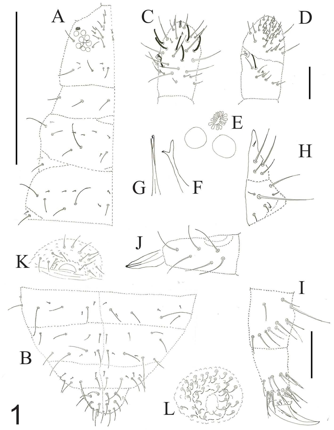
Figure 1. A-L. Pseudachorutes tabasquensis sp. nov. A) Dorsal chaetotaxy from head to Th. III; B) dorsal chaetotaxy from Abd. III. to Abd. VI; C) Ant. III-IV right antenna, dorsal view; D) Ant. III-IV right antenna, ventral view; E) PAO and nearby eyes; F) mandible; G) maxilla; H) labium; I) femur, tibiotarsus, and unguis III; J) dens and mucron; K) female genital plate; L) male genital plate.
Table 1
Pseudachorutes tabasquensis sp. nov. a) Head chaetotaxy, b) dorsal chaetotaxy, c) main characters between P. orghidani, P. conicus, and P. tabasquensis sp. nov.
| 1a. | |||||||
| sd | d | oc | c | p | |||
| Number of setae | 5 | 4+1 | 3 | 1 | 4 | ||
| Setae absent | c1, c3, c4 | ||||||
| 1b. | |||||||
| a | m | p | Setae absent | ||||
| Th. I | – | 3 | – | m2 | |||
| Th. II | 4 | 2 | 5 | a5 | m5 | ||
| Th. III | 3 | 2 | 5 | a2, a5 | m5 | ||
| Abd. I-III | 4 | – | 5 | a2 | |||
| Abd. IV | 4 | – | 6 | ||||
| Abd. V | 4 | – | 4 | ||||
| Abd. VI | 2 | 2 | 2+1 | ||||
| 1c. | |||||||
| Characters | P. conicus | P. tabasquensis sp. nov. | P. orghidani | ||||
| Labium setae L | – | + | ? | ||||
| Ant. IV sensilla | 5 | 6 | 5 | ||||
| Ventral tube setae | 3+3 | 4+4 | ? | ||||
| Mandible teeth | 3 | 2 | 3 | ||||
| Ventral file on Ant. IV | – | 25-30 short setae | 25-30 cuniform | ||||
| Vesicles of PAO | 13-15 | 13-17 | 17 |
Antennae as long as head. Ant. I with 7 setae, Ant. II with 11 setae. Ant. III and IV dorsally fused. Ant. segments ratio I: II: III+IV as 1: 1; 1.8. Ant. III-organ with 2 small straight internal sensilla under a cuticular fold, 2 guard sensilla (sgv about 1.4 times as long as sgd) and 1 microsensillum close to ventral guard sensillum. Ant. IV with trilobed apical bulb, 6 cylindrical sensilla, seta “i”, and one subapical organite (Fig. 1C), ventral file with 25-30 short and strongly spine-like setae (Fig. 1D). PAO elliptical composed of 13-17 simple vesicles, 0.9 times smaller than the nearest eyes (Fig. 1E). 8+8 eyes, F, G are 0.7 times smaller than others. Buccal cone elongated. Mandible with 2 slender teeth (Fig. 1F). Maxilla styliform, with 2 blades, one has an apical tooth, another has 2 apical teeth (Fig. 1G). Labium with normal chaetotaxy of the genus from setae A to G and 4 lateral setae. Setae L spine-shape (Fig. 1H).
Dorsal chaetotaxy as in figure 1A-B, table 1a, b. Seta a0 on the head absent, unpaired seta d1 present, sometimes, one additional seta d3’ between the seta d3 present. Th. I with 3+3 setae, plus 1+1 lateral. Seta a2 present on Th. II, but absent from Th. III to Abd. V. Sensorial setae s on the body in position of p4 and m6 on the thoracic segments II and III, and p5 from Abd. I to IV and p2 on Abd. V. Sensorial formula of the body 022/11111. Sensorial setae 2 times as long as the macrosetae. The ratio of the largest Abd. V setae and inner unguis length is 1.0. Thoracic sterna without setae.
Legs setation from I to III is, tibiotarsi 19, 19, 18, without tenent hairs; Femora 10, 10, 11, one ventro-proximal seta is an acuminate tenent hair; trochanters with 5,5,5; coxae 3, 7, 7; subcoxae 2: 0, 2, 2; subcoxae 1: 1, 2, 2. Unguis wide with one inner tooth near 1/3 part from the basal, and a weakly subbasal lateral tooth. Ratio of tibiotarsus III and unguis about 1.6. Unguiculus absent (Fig. 1I).
Furcula is well developed. Dens dorsally with 6 setae, ventral with a smooth area. Mucro straight, 1.8 times shorter than dens, with granulations and 2 small lamellae (Fig. 1J). Tenaculum with 3+3 teeth. Ventral tube with 4+4 setae. Female genital plate with 3+3 pregenital setae, 6-14 circumgenital setae and 1+1 eugenital setae (Fig. 1K). Male genital plate with 3+3 pregenital setae, 25 circumgenital setae and 4+4 eugenital setae (Fig. 1L).
Taxonomic summary
Type material. Holotype: male mounted on a slide (FC-UNAM: LESM-AC: 23013). 5 paratypes females and 1 juvenile mounted on slides (FC-UNAM: LESM-AC: 23014-23019), same data as holotype.
Type locality. Mexico, Tabasco, Tapijulapa, outside cave “Las Sardinas”, ex litter, 14-III-2002, D.A. Estrada col.
Etymology. The name is locative for the state of Tabasco where the type locality is.
Remarks
Pseudachorutes tabasquensis sp. nov. shares with P. orghidani Massoud & Gruia, 1973 the presence of 1 internal and 1 lateral tooth on unguis. The new species also resembles P. conicus Lee & Kim, 1994 from Korea due to the presence of 2 types of body setae. They all share a similar number of PAO vesicles (Table 1c), dens with 6 setae and tenaculum with 3+3 teeth. Main differences between them are shown in Table 1c. Additionally, P. conicus has a very long and thin unguis, but in P. tabasquensis it is short and thick.
Pseudachorutes mexicanus sp. nov.
(Fig. 2A-K, Table 2a-b)
http://zoobank.org/urn:lsid:zoobank.org:act:96997B68-
7B09-4EC1-9563-2D3DF01AEA77
Description. Body length (n = 17): 814 µm (range: 470-1,350 µm). Color of the body gray-violet, with a dark eyes patch. Granulations are fine and homogenous. Posterior setae of body long and capitated (Fig. 2A).
Antennae as long as head. Ant. I with 7 setae, Ant. II with 11 setae. Ant. III and IV dorsally fused. Ant. segments ratio I: II; III+IV as 1: 1.4; 3.2. Ant. III-organ with 2 small straight internal sensilla under a cuticular fold, 2 guard sensilla (sgv about 1.2 times as long as sgd) and 1 microsensillum close to ventral guard sensillum. Ant. IV with simple apical bulb, 6 cylindrical sensilla, seta “i”, 1 microsensillum and 1 subapical organite (Fig. 2B), ventral file poorly developed, with 20-35 short setae (Fig. 2C). PAO elliptical composed of 5-6 simple vesicles, 1.1 times as long as the nearest ocelli (Fig. 2D). 8+8 small ocelli, F, G are 0.9 times smaller than others. Buccal cone short. Mandible with 2 slender teeth (Fig. 2E). Maxilla with 2 blades, each has 2 apical teeth (Fig. 2F). Labium with normal chaetotaxy of the genus from setae A to G and 4 lateral setae, setae L spine-shape (Fig. 2G).
Dorsal chaetotaxy as in figure 2A, table 2b. Seta a0 on head absent, unpaired seta d1 present. Th. I with 3+3 setae. Setae a2 present on Th. II, but absent from Th. III to Abd. V. Sensory setae s on the body in position of p4 and m6 on Th. II and III, and p5 from Abd. I to IV and p2 on Abd. V. Sensorial formula of the body 022/11111. Sensory setae longer than 1.1-1.5 times as long as body setae. Ratio of largest Abd. V setae and inner unguis length is 1.4. Thoracic sterna without setae. Ventral tube with 4+4 setae. Female genital plate with 2+2 pregenital setae, 4-9 circumgenital setae and 1+1 eugenital setae (Fig. 2H). Male genital plate with 3+3 pregenital setae, 10 circumgenital setae and 4+4 eugenital setae (Fig. 2I).
Tibiotarsi I, II, III with 18, 18, 17 setae respectively, with 1 tenent hair long and capitate (Fig. B8). Femora I, II, III with 9, 9, 10 setae respectively. Trochanters with 5 setae each. Coxae I, II, III with 3, 7, 7 setae respectively. Subcoxae 2 I, II, III with 0, 2, 2 setae respectively. Subcoxae 1. I, II, III with 1, 2-3, 2-3 setae respectively. Unguis wide with 1 weakly apical inner tooth. Ratio of tibiotarsus III and unguis about 1.0. Unguiculus absent (Fig. 2J).
Furcula well developed. Dens dorsally with 5 setae. Mucro straight, 3 times shorter than dens, with two larger bladder-like swelling visible and a hook-like end (Fig. 2K). Tenaculum with 3+3 teeth.

Figure 2. A-K. Pseudachorutes mexicanus sp. nov. A) Dorsal chaetotaxy from head to abdomen VI; B) Ant. III-IV right antenna, dorsal view; C) Ant. III-IV right antenna, ventral view; D) PAO and nearby eye; E) mandible; F) maxilla; G) labium; H) female genital plate; I) male genital plate; J) femur, tibiotarsus, and unguis III; K) furcula and tenaculum.
Taxonomic summary
Type material. Holotype: female mounted on a slide (FC-UNAM: LESM-AC: 22996). 16 paratypes: 4 females, 1 male and 11 juveniles under slides (FC-UNAM: LESM-AC: 22997-23012), same data as holotype.
Type locality. Mexico, Hidalgo, Mineral El Chico, 10-IX-98, J.A. Monterrubio, col. Ex Tillandsia violacea.
Etymology. The name of the new species is after the country of the type locality: Mexico.
Remarks
This species resembles P. americanus Stach, 1949 with a similar number of vesicles in PAO (P. americanus with 5-8 vesicles), unguis with 1 minute tooth near apex, one large, clavate tenent hair, ventral tube with 4+4 setae, tenaculum with 3+3 teeth and posterior abdominal setae clearly capitate. However, dens of the new species with 5 setae, maxilla with 2 blades and each has 2 apical teeth, 6 cylindrical sensilla on Ant. IV and a poorly developed ventral file with 20-35 short setae is different from P. americanus.
Pseudachorutes chichinautzin sp. nov.
(Fig. 3A-J, Table 3a-c)
http://zoobank.org/urn:lsid:zoobank.org:act:1098FF48-F5CE-4D51-8F9E-0EB9E217AA40
Description.Body length (n = 8): 1,904 µm (range: 850-2,010 µm). Color of the body gray-violet, with a dark eyes patch. Granulations homogenous. Lateral and posterior body setae are longer and truncate (Fig. 3A).
Table 2
Pseudachorutes mexicanus sp. nov. a) Head chaetotaxy, b) dorsal chaetotaxy.
| 2a. | ||||||
| sd | d | oc | c | p | ||
| Number of setae | 5 | 4+1 | 3 | 4 | 4 | |
| 2b. | ||||||
| a | m | p | Setae absent | |||
| Th. I | – | 3 | – | m2 | ||
| Th. II | 4 | 3 | 5 | a4 | ||
| Th. III | 3 | 3 | 5 | |||
| Abd. I-III | 3 | 2 | 5 | |||
| Abd. IV | 4 | – | 5 | |||
| Abd. V | 3 | – | 4 | |||
| Abd. VI | 2 | 2 | 2+1 |
Antennae as long as head. Ant. I with 7 setae, Ant. II with 12 setae. Ant. III and IV dorsally fused. Ant. segments ratio I: II; III+IV as 1: 1.2: 2.0. Ant. III-organ with 2 small internal sensilla under a cuticular fold, 2 guard sensilla (sgv about 1.1 times as long as sgd) and 1 microsensillum close to ventral guard sensillum. Ant. IV with trilobed apical bulb, 6 cylindrical sensilla, seta “i”, and one subapical organite (Fig. 3B), ventral file with about 10 strong, spine-like setae and several slender, normal setae (Fig. 3C). Some setae on Ant. IV are blunt. PAO elliptical composed of 10-12 vesicles, sometimes, 1 or 2 of them inside in the others, subequal to nearest eyes (Fig. 3D). 8+8 eyes, F, G are 0.7 times smaller than others. Buccal cone elongated. Mandible is not clearly detected, about 2 or 3 slender teeth. Maxilla with 2 blades and one has an apical tooth, and the other styliform (Fig. 3E). Labium with normal chaetotaxy of the genus from setae A to G and 5 lateral setae, setae L spine-shape (Fig. 3F).
Dorsal chaetotaxy as in Fig. 3A, table 3a, b. Seta a0 on the head absent, unpaired seta d1 present. Th. I with 3+3 setae, plus 1+1 lateral. Setae a2 present on Th. II, but absent from Th. III to Abd. V. Sensorial setae s on the body in position of p4 and m6 on the thoracic segments II and III, and p5 from Abd. I to IV and p3 on Abd. V. Sensorial formula of the body 022/11111. Sensorial setae 1.2-1.7 times as long as the normal setae. The lateral setae of the body longer and blunt. Ratio of largest Abd. V setae and inner unguis length is 1.0. Thoracic sterna without setae. Ventral tube with 4+4 setae. Female genital plate with 3+3 pregenital setae, 9 circumgenital setae and 1+1 eugenital setae (Fig. 3G). Male genital plate with 3+3 pregenital setae, 8 circumgenital setae and 4+4 eugenital setae (Fig. 3H).
Leg setation from I to III, is tibiotarsi 19, 19, 18, with 1 acuminate tenent hair a little longer than others; femora 9, 9,10, one ventro-proximal seta is an acuminate tenent hair; trochanters with 5,5,5; coxae 3, 7, 7; subcoxae 2: 0, 2, 2; subcoxae 1: 1, 2, 2. Unguis wide, with one inner tooth near 1/3 part from the basal. Sometimes, a pair of weakly subbasal lateral tooth is present. Ratio of tibiotarsus III and unguis about 1.6. Unguiculus absent (Fig. 3I).

Figure 3. A-J. Pseudachorutes chichinautzin sp. nov. A) Dorsal chaetotaxy; B) Ant. III-IV right antenna, dorsal view; C) Ant. III-IV right antenna, ventral view; D) PAO, eye patch and ocular setae; E) maxilla; F) labium; G) female genital plate; H) male genital plate; I) femur, tibiotarsus, and unguis III; J) furcula and tenaculum.
Furcula well developed. Dens dorsally with 6 setae, ventral with fine granulate. Mucro straight, 1.7 times shorter than dens, with 2 big lamella and a clearly hook-like end. Tenaculum with 3+3 teeth (Fig. 3J).
Taxonomic summary
Material examined. Holotype: female under slide (FC-UNAM: LESM-AC: 22974). 7 paratypes: 4 females, 2 males and 1 juvenile under slides, same data as holotype (FC-UNAM: LESM-AC: 22975-22981).
Type locality. Mexico; Morelos, Derrame Chichinautzin. 12-IX-1976. J. Palacios, col. Ex. Tillandsia prodigiosa.
Etymology. The name is that of the Chichinautzin lava flow (state of Morelos), as a noun of type locality.
Remarks
Pseudachorutes chichinautzin sp. nov. shares with P. orghidani and P. subcrassus Tullberg, 1871 the presence of 1 internal and 1 pair of lateral teeth on unguis. The new species also resembles P. tabasquensis sp. nov. with 2 types of body setae, Ant. IV with 6 sensilla, trilobed apical bulb. Dens with 6 setae and tenaculum with 3+3 teeth. Main differences between them can be seen in table 3c.
Table 3
Pseudachorutes chichinautzin sp. nov. a) Head chaetotaxy, b) dorsal chaetotaxy, c) main characters between P. orghidani, P. subcrassus, P. chichinautzin sp. nov. and P. tabasquensis sp. nov.
| 3a. | ||||||
| sd | d | oc | c | p | ||
| Number of setae | 5 | 4+1 | 3 | 2 | 4 | |
| Setae absent | c1, c4 | |||||
| 3b. | ||||||
| a | m | p | Setae absent | |||
| Th. I | – | 3 | – | m2 | ||
| Th. II | 4 | 2 | 5 | a5 | m4 | |
| Th. III | 3 | 2 | 5 | a2, a5 | m4 | |
| Abd. I-III | 3 | – | 5 | a2, a5 | ||
| Abd. IV | 3 | – | 5 | a2, a3, a5 | ||
| Abd. V | 3 | – | 3 | a2 | P2 | |
| Abd. VI | 2 | 2 | 2+1 | |||
| 3c. | ||||||
| Characters | P. subcrassus | P. chichinautzin sp. nov. | P. tabasquensis sp. nov. | P. orghidani | ||
| Ant. IV sensilla | 5-6 | 6 | 6 | 5 | ||
| Mandible teeth | 4 | 2-3 | 2 | 3 | ||
| Ventral file on Ant. IV | 20 | 10 strong setae | 25-30 short setae | 25-30 cuniform | ||
| Vesicles of PAO | 8-10 | 10-12 | 13-17 | 17 | ||
| Lateral blunt setae | – | + | – | + |
Pseudachorutes tillandsiodes sp. nov.
(Fig. 4A-K, Table 4a-c)
http://zoobank.org/urn:lsid:zoobank.org:act:9FFB9169-78E7-4BA3-8C9A-8F3EBEA4DD10
Description. Body length (n = 6): 2,260 µm (range: 1,750-2,860 µm). Color of the body violet, with a white strip from Th. I to Th. II and a dark eyes patch. Granulations fine and homogenous. Body with simple and spine-like setae, p row longer on last abdominal segments (24-40 µm), long sensorial setae (75-100 µm) (Fig. 4A, B).
Antennae shorter than head, 155 µm and 180 µm respectively. Ant. I with 7 setae Ant. II with 12 setae. Ant. III and IV dorsally fused. Ant. segments ratio I: II; III+IV as 1: 1; 1.9. Ant. III-organ with 2 small curving sensilla under a cuticular fold, 2 guard sensilla (sgv is about 1.4 times as long as sgd) and 1 microsensillum close to ventral guard sensillum. Ant. IV with trilobed apical bulb, 6 thin and cylindrical sensilla, seta “i”, one microsensillum and one subapical organite (Fig. 4C), ventral side with about 20 setae with some thick and spine-like (Fig. 4D). PAO elliptical composed of 14 vesicles, 1.2 times as long as the nearest eyes. 8+8 eyes, F, G 0.9 times as big as others (Fig. 4E). Buccal cone elongated. Mandible has 2 big teeth, the apical with clearly 3 small teeth (Fig. 4F). Maxilla with 2 blades, one with 2 apical teeth (Fig. 4G). Labium with normal chaetotaxy of the genus from setae A to G and 4 lateral setae, setae L reduced to a minus spine, difficult to see (Fig. 4H).
Dorsal chaetotaxy as in figure 4A, B, table 4a, b. Seta a0 on head absent, unpaired seta d1 present. Th. I with 3+3 setae. Setae a2 present on Th. II, but absent from Th. III to Abd. V. m5 present on Th. II to Th. III. Sensorial setae on body in position of p4 and m6 on thoracic segments II and III, p5 from Abd. I to IV and p2 on Abd. V. Sensorial formula of the body 022/11111. Sensorial setae 2.5-4.0 times as long as the normal setae. Ratio of largest Abd. V setae and inner unguis length is 0.6. Thoracic sterna without setae. Ventral tube with 4+4 setae. Female genital plate with 3+3 pregenital setae, 9 circumgenital setae and 1+1 eugenital setae (Fig. 4I). No males were found.

Figure 4. A-K. Pseudachorutes tillandsiodes sp. nov. A) Dorsal chaetotaxy from head to Th. III; B) dorsal chaetotaxy from Abd. III. to Abd. VI; C) Ant. III-IV right antenna, dorsal view; D) Ant. III-IV right antenna, ventral view; E) PAO, eye patch and ocular setae; F) mandible; G) maxilla; H) labium; I) female genital plate; J) femur, tibiotarsus, and unguis III; K) dens and mucron.
Leg setation from I to III, is tibiotarsi 19, 19, 18, no tenent hair; femora 9, 10, 10, one ventro-proximal seta is an acuminate tenent hair; trochanters with 5,5,5; coxae 3, 7, 8; subcoxae 2: 0, 2, 2; subcoxae 1: 1, 2, 2. Unguis with one clearly inner tooth at the basal side. Ratio of tibiotarsus III and unguis about 1.5. Unguiculus absent (Fig. 4J).
Furcula well developed. Dens dorsally with 6 setae, ventral with fine granulations. Mucro straight, 2.2 times shorter than dens, with 2 thin but long lamella, without hook-like end (Fig. 4K). Tenaculum with 3+3 teeth.
Table 4
Pseudachorutes tillandsiodes sp. nov. a) Head chaetotaxy, b) dorsal chaetotaxy, c) main characters between P. gilvusi, and P. tillandsiodes sp. nov.
| 4a. | ||||||
| sd | d | oc | c | p | ||
| Number of setae | 5 | 4+1 | 3 | 4 | 4 | |
| 4b. | ||||||
| a | m | p | Setae absent | |||
| Th. I | – | 3 | – | m2 | ||
| Th. II | 5 | 2 | 5 | m4 | ||
| Th. III | 4 | 2 | 5 | a2 | m4 | |
| Abd. I-III | 4 | – | 5 | a2 | ||
| Abd. IV | 4 | – | 5 | a2 | ||
| Abd. V | 4 | – | 3 | P4 | ||
| Abd. VI | 2 | 2 | 2+1 | |||
| 4c. | ||||||
| Characters | P. gilvus | P. tillandsiodes sp. nov. | ||||
| Setae d1 on head | 1+1 | 1 | ||||
| Setae number on Th. I | 2+2 | 3+3 | ||||
| Setae a2 on Th. II | – | + | ||||
| Ant. IV sensilla | 7 | 6 | ||||
| Ventral tuve setae | 3+3 | 4+4 |
Taxonomic summary
Material examined. Holotype: female under slide (FC-UNAM: LESM-AC: 23172). 5 Paratypes: 4 female and 1 juvenile (FC-UNAM: LESM-AC: 23173-23177).
Type locality. Mexico; Hidalgo, Mineral El Chico. 10-IX-98. J. A. Monterrubio, col. Ex Tillandsia violacea.
Etymology. The name is taken from the epiphytic genus Tillandsia (Bromeliacea) habitat where the species was found.
Remarks
Pseudachorutes tillandsiodes sp. nov. resembles P. gilvus Oliveira & Deharveng, 1995 with white strips and long sensilla on the body, similar number of postantennal organ vesicles (P. gilvus with 11-15 vesicles), unguis with 1 inner tooth, tibiotarsi I-III with 19, 19, 18 setae and dens with 6 setae. The main differences between them are shown in table 4c. However, P. gilvus has 3 white stripes on the body: the first on the posterior part of head and the middle of Th. I, the second on the mesothorax and the third on Abd. I-II; P. tillandsiodes sp. nov. only with 1 white stripe from Th. I to Th. II.
Pseudachorutes veracruzensis sp. nov.
(Fig. 5A-L, Table 5a, b)
http://zoobank.org/urn:lsid:zoobank.org:act:2C15B37C-080B-4DF9-AD8E-9AE899AEA907
Material examined. Holotype: female under slide (FC-UNAM: LESM-AC: 2133a). 10 paratypes: 7 females and 3 males under slides, same data as holotype (FC-UNAM: LESM-AC: 2131a-2132c, 2132a-2132e, 2133b, 2133c)
Type locality. Mexico; Veracruz, Xalapa, La Herradura. 26-IX-26-10/1998, ex Bosque Mesófilo de Montaña, J. Márquez, col.
Description. Body length (n = 11): 1,900 (range: 1,050-3,400 µm). Color body violet, with a dark eyes patch. Granulations fine and homogenous. Body with short and simple setae (10-12), some of them longer in abdomen segments, especially on 4th segment (22-26 µm), long sensorial setae (67-75 µm) (Fig. 5A).
Antennae little shorter than head, 100 µm and 105 µm, respectively. Ant. I with 7 setae, Ant. II with 12 setae. Ant. III and IV dorsally fused. Ant. segments ratio I: II; III+IV as 1: 1; 2. Ant. III-organ with 2 small straight sensilla under a cuticular fold, 2 guard sensilla (the sgv is about 1.1 times as long as sgd) and 1 microsensillum close to ventral guard sensillum. Ant. IV dorsally with trilobed apical bulb, 6 thin and cylindrical sensilla, seta “i”, 1 microsensillum and 1 subapical organite (Fig. 5B), ventral side has a distinct ventral file with about 40 short setae (Fig. 5C). PAO elliptical composed of 17-20 vesicles, 1.5 times as long as the nearest eyes. 8+8 eyes, F, G 0.8 times as big as others (Fig. 5D). Buccal cone elongated. Mandible has 2-3 big teeth (Fig. 5E). Maxilla with 1 blade and 2 apical teeth (Fig. 5F). Labium with normal chaetotaxy of the genus from setae A to G and 3 lateral setae, one longer spine-like setae present at the place of setae L (Fig. 5G).
Dorsal chaetotaxy as in figure 5A and table 5a,b. Seta a0 on head absent, unpaired seta d1 present. Th. I with 3+3 setae. Setae a2 present on Th. II, but absent from Th. III to Abd. IV. m5 present on Th. II to Th. III. Sensorial setae s on the body in position of p4 and m6 on Th. II and III, p5 from Abd. I to IV and p2 on Abd. V. Sensorial formula of the body 022/11111. Sensorial setae 6.5-7.0 times as long as the shorter setae. The ratio of the largest Abd. V setae and inner unguis length is 0.5. Thoracic sterna without setae. Ventral tube with 4+4 setae. Female genital plate with 3+3 pregenital setae, 7 circumgenital setae and 1+1 eugenital setae (Fig. 5H). Male genital plate with 2+2 pregenital setae, 16 circumgenital setae and 4+4 eugenital setae (Fig. 5I).
Leg setation from I to III, is tibiotarsi 19, 19, 18, no tenent hairs; femora 13, 11, 10, one ventro-proximal seta is an acuminate tenent hair; trochanters with 6,6,5; coxae 3, 7, 8; subcoxae 2: 0, 2, 2; subcoxae 1: 1, 2, 2. Unguis with 1 big and 1 small inner tooth together with 2 pairs of lateral teeth (Fig. 5J). Ratio of tibiotarsus III and unguis about 1.4. Unguiculus absent (Fig. 5K).
Furcula well developed. Dens dorsally with 6 setae, ventral granulate. Mucron granulated with broad and long lamella, 1 slightly hook-like end, 2.0 times shorter than dens (Fig. 5L). Tenaculum with 3+3 teeth.
Etymology. The name is a locative for the State of Veracruz where the type locality is found.
Remarks
Pseudachorutes veracruzensis sp. nov. resembles P. orghidani with granules on mucron and dens with 6 setae, mandible with 3 teeth, unguis with lateral teeth, similar number of PAO (P. orghidani with 17 vesicles) and ventral file on Ant. IV. The main difference between the species is the shape of short setae in the ventral file (P. orghidani has small setae with apex truncate) and number of sensilla on Ant. IV (P. orghidani with 5) and the teeth on unguis (P. orghidani only with 1+1 lateral teeth).
Discussion
After revision and analysis of the material deposited in the LESM collection, we were able to update the knowledge of genus Pseudachorutes in Mexico, describing 5 new species: P. tabasquensis sp. nov., P. veracrucensis sp. nov., P. tillandsiodes sp. nov., P. chichinautzin sp. nov., and P. mexicanus sp. nov. Three new records for the country are added, for the following species: P. ca. algidensis from Hidalgo, P. ca. crassus from Estado de México, these must be confirmed with the collection of more specimens that will allow the species to be fully determined. For now, this information is presented as an element to show the richness of species of the genus in the country. Pseudachorutes reductus has a distribution in the Antilles and southern Florida, the new records in Mexico extend its distribution area and confirm the affinity of the species to the Atlantic area. Total records for Pseudachorutes is increased to 28 species, from 20 states and 62 localities within the country. Quintana Roo and Hidalgo were the states with the highest number of species present (11 and 10, respectively), followed by Morelos, Estado de México, Puebla, Veracruz, and Guerrero (8, 7, 6, 6, and 4 species recorded in each one), 6 states have 3 species, 5 have 2 and Querétaro and San Luis Potosí only have 1 species recorded. Three species are widely distributed in Mexico: P. corticolus, P. simplex, and P. subcrassoides. Diversity of the genus in Mexico is around 21% of the total known worldwide, and therefore the country becomes one with the greatest number of species present.
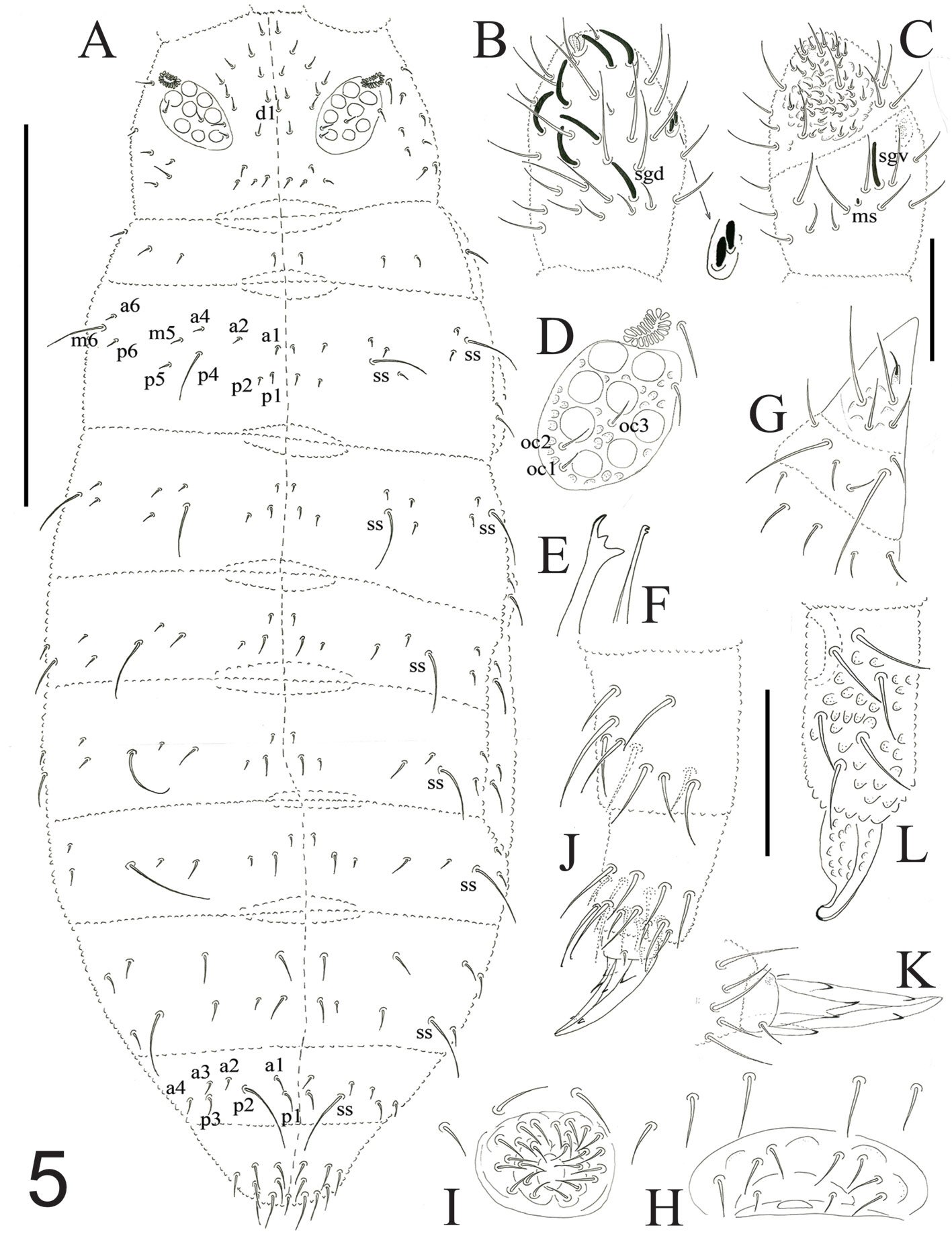
Figure 5. A-L. Pseudachorutes veracruzensis sp. nov. A) Dorsal chaetotaxy; B) Ant. III-IV right antenna, dorsal view; C) Ant. III-IV right antenna, ventral view; D) PAO, eye patch and ocular setae; E) mandible; F) maxilla; G) labium; H) female genital plate; I) male genital plate; J) femur, tibiotarsus, and unguis III; K) unguis III, ventral view; L) dens and mucron.
Regarding biotopes where the species preferably live, we found that litter, epiphytic plants, soil, mosses and decaying wood are the most suitable habitats for this springtail. However, sand, canopy, wood, caves and anthills are also microhabitats used by some species.
Table 5
Pseudachorutes veracruzensis sp. nov. a) Head chaetotaxy, b) dorsal chaetotaxy.
| 5a. | |||||
| sd | d | oc | c | p | |
| Number of setae | 5 | 4+1 | 3 | 2 | 4 |
| Setae absent | c1, c3 c4 | ||||
| 5b. | |||||
| a | m | p | Setae absent | ||
| Th. I | – | 3 | – | m2 | |
| Th. II | 4 | 2 | 5 | a5 | m4 |
| Th. III | 3 | 2 | 5 | a2, a5 | m4 |
| Abd. I-III | 3 | – | 5 | a2, a5 | |
| Abd. IV | 4 | – | 5 | a2, a3 | |
| Abd. V | 3 | – | 4 | a4 | |
| Abd. VI | 3 | 2 | 2+1 |
The analysis and revision of the morphology of the 5 species described, allowed us to come to the following conclusions about the morphology of the genus that needs to be taken in consideration. Size of body setae should be a characteristic to be taken into consideration for the description of the species, since we observed that it is a variable character. Antennae are a uniform structure and characters associated with the sensory organ of Ant. III have little relevance at a specific level. Sensory file of Ant. IV, present a varied shape and number, from 8 to 40 setae. Apical vesicle of Ant. lV is trilobed in most species and others have a simple shape. Number of ocelli is stable within the genus, presenting 8+8. The maxillae and mandibles vary in all species. Maxillae can be needle-shaped, crocheted or styliform, they may or may not be lamellar and the number of lamellae is variable, and in most cases, there are 1 to 2 apical teeth. The number of teeth in the mandibles in almost all species ranges from 1 to 5. The number of teeth in the retinaculum is a constant character among the species of the genus, with 3+3 teeth. The ventral tube in almost all species has 4+4 setae. The number of setae in the dens varies from three to seven, but most have six setae. The mucron has 2 lamellae in all species, except in P. reductus, where it is greatly reduced. The shape of the mucron is variable, from elliptical, triangular, elongated, short, curved, widened, or with a bladder-shaped base.
Acknowledgments
This study had the support from the International Relationships of Universidad Nacional Autónoma de México issued to the first author and partially by the National Natural Sciences Foundation of China (No. 3217047 and 32370491). Blanca E. Mejía Recamier helped remount specimens. Kenneth A. Christiansen gave criticism, suggestions, and literature. We thank Erick García and Eduardo Pacheco who assigned the catalogue numbers for the slides. Daniel A. Estrada, Jesús A. Monterrubio, Juan Márquez donated the specimens.
References
Arango-Galván, A., Cutz-Pool, L. Q., & Cano-Santana, Z. (2007). Estructura de la comunidad de colémbolos del mantillo de la Reserva Ecológica del Pedregal de San Ángel: Riqueza, composición y abundancia relativa. Entomología Mexicana, 6, 397–400.
Bellinger, P. F., Christiansen, K. A., & Janssens, F. (2023). Checklist of the Collembola of the World. Retrieved on November 11th, 2023 from: http://www.collembola.org
Christiansen, K. A., & Bellinger, P. F. (1998). The Collembola of North America, North of the Río Grande: a taxonomic analysis. Part I. Grinnell, Iowa Grinnell College.
Cutz-Pool, L. Q., Palacios-Vargas, J. G., & Vázquez, M. M. (2003). Comparación de algunos aspectos ecológicos de Collembola en cuatro asociaciones vegetales de Noh-Bec, Quintana Roo, México. Folia Entomológica Mexicana, 42, 91–101.
Cutz-Pool, L. Q., García-Gómez, A., & Palacios-Vargas, J. G. (2007a). Primer estudio de colémbolos (Hexapoda: Collembola) de la Hoya de las Guaguas en el estado de San Luis Potosí, México. Dugesiana, 14, 47–51.
Cutz-Pool, L. Q., Palacios-Vargas, J. G., Castaño-Meneses, G., & García-Calderón, N. E. (2007b). Edaphic Collembola from two agroecosystems with contrasting irrigation type in Hidalgo State, Mexico. Applied Soil Ecology, 36, 46–52. https://doi.org/10.1016/j.apsoil.2006.11.009
Cutz-Pool, L. Q., Palacios-Vargas, J. G., & Castaño-Meneses, G. (2008). Estructura de la comunidad de colémbolos (Hexapoda: Collembola) en musgos corticícolas en un gradiente altitudinal de un bosque templado subhúmedo. Revista de Biología Tropical, 56, 1–10. https://doi.org/10.15517/rbt.v56i2.5620
Fjellberg, A. (1998). Fauna entomologica scandinavica. The Collembola of Fennoscandia and Denmark. Part I: Poduromorpha. Vol. 35. Leiden: Brill Publishers.
Jordana, R., Arbea, J. I., Simón, C., & Luciáñez, M. J. (1997). Fauna ibérica. Vol. 8. Collembola, Poduromorpha. Madrid: Museo Nacional de Ciencias Naturales.
Palacios-Vargas, J. G. (1990). Manuales y guías para el estudio de microartrópodos I. Diagnosis y clave para determinar las familias de los Collembola de la Región Neotropical. México D.F.: Facultad de Ciencias, Universidad Nacional Autónoma de México.
Palacios-Vargas, J. G. (1997). Catálogo de los Collembola de México. Las Prensas de Ciencias, UNAM, México D.F.
Palacios-Vargas, J. G. (2005). Collembola. In G. Sánchez-Ramos, P. Reyes-Castillo y R. Dirzo (Eds.), Historia natural de la Reserva de la Biosfera El Cielo Tamaulipas, México (pp. 354–366). Ciudad Victoria, Tamaulipas: Universidad Autónoma de Tamaulipas.
Palacios-Vargas, J. G., & Castaño-Meneses, G. (2003). Seasonality and community composition of springtails in Mexican forests. In Y. Basset, V. Novotny, S. E. Millar, & R. L. Kitching (Eds.), Arthropods of tropical forests. Spatio-temporal dynamics and resource use in the canopy (pp. 159–169). Cambridge, UK: Cambridge University Press.
Palacios-Vargas, J. G., Castaño-Meneses, G., & Mejía-Recamier, B. E. (2000). Collembola. In J. Llorente-Bousquets, E. González-Soriano, & N. Papayero (Eds.), Biodiversidad, taxonomía y biogeografía de artrópodos de México. Hacia una síntesis de su conocimiento II (pp. 249–273).México D.F.: Las Prensas de Ciencias, UNAM.
Palacios-Vargas, J. G., Cutz-Pool, L. Q., & Estrada-Barcenas, D. A. (2007). Collembola. In I. Luna, J. J. Morrone, & D. Espinosa (Eds.). Biodiversidad de la Faja Volcánica Transmexicana (pp. 331–344).México D.F.: Las Prensas de Ciencias, UNAM.
Tullberg, T. (1871). Förteckning öfver Svenska Podukrider. Öfversigt af Kongliga Vetenskaaps -Akademiens Förhandlingar, 28, 143–155.
Vázquez, M. M. (1988). Fauna colembológica de hojarasca y suelo. In L. Arriaga, & A. Ortega (Eds.), La sierra de la Laguna de Baja California Sur (pp. 133–148). La Paz, Baja California Sur: Centro de Investigaciones Biológicas de Baja California Sur, A.C.
Vázquez, M. M., & Palacios-Vargas, J. G. (1990). Nuevos registros y aspectos biogeográficos de los colémbolos de la sierra de la Laguna, B. C. S., México. Folia Entomológica Mexicana, 78, 5–22.
Vázquez, M. M., & Palacios-Vargas, J. G. (2004). Catálogo de colémbolos (Hexapoda: Collembola) de Sian Ka’an, Quintana Roo, México. México D.F.: Universidad de Quintana Roo/ Comisión Nacional para el Conocimiento y Uso de la Biodiversidad.

Las abejas sin aguijón (Apidae: Apinae: Meliponini) de Bolivia: una aproximación al conocimiento sobre su riqueza y distribución geográfica
Ariel Ángel Céspedes-Llave *
Universidad San Francisco Xavier de Chuquisaca, Facultad Ciencias Químico Farmacéuticas y Bioquímicas, Experimental de Biología “Luis Adam Brianςon”, Calle Dalence Núm. 51, Ciudad de Sucre, Chuquisaca, Bolivia
*Autor para correspondencia: cespedes.ariel@usfx.bo (A.A. Céspedes-Llave )
Recibido: 6 febrero 2024; aceptado: 11 abril 2024
Resumen
El objetivo principal de este trabajo fue generar una lista actualizada de las especies de abejas sin aguijón (Apidae: Apinae: Meliponini) en Bolivia, abordando aspectos geográficos, taxonómicos, históricos y ecorregionales. Se realizaron ajustes en la sistemática de abejas sin aguijón y correcciones geográficas mediante un minucioso análisis de la información recopilada. Los resultados obtenidos muestran la presencia de 121 especies en Bolivia, distribuidas en 19 géneros válidos, estos datos se basan en 616 registros recopilados desde 1932 hasta 2022, se destaca que la riqueza de especies de las abejas meliponinas es notablemente alta por debajo de 1,000 m (> 90% especies). Las ecorregiones más diversas resultaron ser los Yungas y el sudoeste de la Amazonia albergando 90% de las especies. Con este trabajo, se logró generar datos actualizados de la riqueza de especies de meliponinos con información de distribución geográfica para Bolivia. La relevancia de este estudio es impulsar la consolidación de conocimientos de diversidad de abejas, con el involucramiento de instituciones científicas y la comunidad investigadores. Además, que sirva como guía para las meliponiculturas locales, para identificar y manejar especies en función de la ecorregión en la que se ubiquen.
Palabras clave: Estado de conocimiento; Meliponinos; Registros geográficos; Registros taxonómicos
© 2024 Universidad Nacional Autónoma de México, Instituto de Biología. Este es un artículo Open Access bajo la licencia CC BY-NC-ND
(http://creativecommons.org/licenses/by-nc-nd/4.0/).
Stingless bees (Apidae: Apinae: Meliponini) from Bolivia: an approach to the richness and geographical distribution
Abstract
The aim of this study was to compile an updated species inventory of stingless bees (Apidae: Apinae: Meliponini) in Bolivia, considering geographic, taxonomic, historical and ecoregional aspects. Adjustments in the systematics of stingless bees and geographic data corrections were made through exhaustive analysis of the available information. The results reveal the presence of 121 species in Bolivia, distributed in 19 valid genera, these findings are based on 616 records spanning from 1932 to 2022. Notably, the species richness of meliponinos bee’s is particularly high below 1,000 meters (> 90% species). The Yungas and southwestern Amazonia were identified as the most diverse ecoregion, with 90% of the species. This study´s significance lies in advancing the understanding of the bee diversity, and fostering collaboration among institutions and researcher community. Moreover, the gathered information aims to support meliponiculture initiatives by helping stakeholders identify and manage species within their respective ecoregion.
Keywords: Knowledge status; Meliponine bees; Geographic records; Taxonomic records
Introducción
La familia Apidae (Hymenoptera) abarca una amplia diversidad de linajes de abejas antófilas, entre los que se encuentran las abejas sin aguijón, también conocidas como meliponinos (término acuñado por Moure (1963)). Desde el punto de vista taxonómico pertenecen a la tribu Meliponini, cuyo nombre deriva del griego meli (μέλι) = miel, ponos (πόνος) = trabajo y el sufijo ini = que indica o agrupa como tribu a los animales. Estas abejas juegan un papel ecológico muy importante en la polinización en ambientes naturales y agroecosistemas, lo que las hace cruciales para mantener la salud de los ecosistemas y la seguridad alimentaria (González et al., 2018; Layek et al., 2022; Slaa et al., 2006). A nivel global constituyen más de 500 especies con distribución pantropical o subtropical (Hrncir et al., 2016; Michener, 2013) y en la región neotropical se tienen registradas más de 400 especies (Camargo et al., 2013; Freitas et al., 2009; Michener, 2013), llegando a representar la mayor riqueza (~ 80%) de todas las especies de abejas sin aguijón.
Los meliponinos se encuentran distribuidos en áreas tropicales y subtropicales en América, es decir, abarcando desde el norte de México hasta el norte de Argentina (Camargo et al., 2013). La mayor riqueza de especies en América del Sur se encuentra en Brasil con un impresionante registro de 259 especies (Nogueira, 2023; Pedro, 2014). Le sigue Perú, con 175 especies documentadas (Rasmussen y Castillo, 2003; Rasmussen y Delgado, 2019) y Ecuador con 132 especies (Vit et al., 2018). Colombia con una notable diversidad de 129 especies (Nates-Parra, 2001; Nates-Parra y Rosso-Londoño, 2013), mientras que Venezuela reporta 83 especies (Pedro y Camargo, 2013). La Guyana Francesa ha registrados 80 especies (Pauly et al., 2013) y Argentina está experimentado avances significativos en sus inventarios pasando de 33 a 37 especies catalogadas (Álvarez, 2015; Lucia y Álvarez, 2023). Este panorama subraya la importancia de la investigación continua para comprender y preservar la rica diversidad de las abejas sin aguijón en la región neotropical.
Los primeros registros de especies de abejas sin agujón para Bolivia, datan de los trabajos pioneros de Cockerell (1919), Schwarz (1932, 1948), Moure (1950), Wille (1960) y Kempf-Mercado (1962, 1968). Sin embargo, uno de los hitos más significativos en la recopilación del conocimiento de abejas sin aguijón en la región neotropical, es la publicación del catálogo de abejas de Moure et al. (2007). Este catálogo es un referente y revela que para Bolivia, la riqueza de especies de abejas sin aguijón está compuesta por 21 géneros y 88 especies (Camargo y Pedro 2007; Camargo et al., 2013). Asimismo, actualmente se disponen de otras plataformas de libre acceso, que ofrecen registros de abejas para Bolivia. Entre éstas, se destacan World Bee Diversity (Ascher y Pickering, 2020), la Asociación Brasileira de Estudios de las Abejas (A.B.E.L.H.A., 2016) y el Global Biodiversity Information Facility (GBIF, 2023). Estas plataformas son una fuente valiosa para complementar y actualizar la información sobre la diversidad de abejas sin aguijón en el contexto boliviano.
El conocimiento de la riqueza de especies también se benefició de iniciativas en el ámbito de la meliponicultura, con diversos proyectos que se gestaron a partir de la década de los 90 (Aguilera, 2019). Estos proyectos incluyen iniciativas como las llevadas a cabo en el departamento del Beni, específicamente dentro de comunidades indígenas Sirionó de Ibiato (Montaño, 1996). Asimismo, en Santa Cruz se implementaron proyectos a partir del 2000 en comunidades indígenas guaraní y quechuas, como se documenta en los trabajos de Martínez y Cuéllar (2004), Ferrufino y Aguilera (2006) y Aguilera (2019). Otras experiencias valiosas se dieron en las comunidades indígenas de Tacana en La Paz (Alipaz et al., 2006), durante el 2010 en Tarija, en regiones del Chaco (Clemente y Lahore, 2010), en Cochabamba las comunidades indígenas yuracares (GADC/ALD, 2014) y en Chuquisaca, a partir de 2015, con la formación de asociaciones de meliponicultoras(es) (Campos y Peducassé, 2017; Delgado y Martínez, 2021; PASOS, 2015). Actualmente, se observan esfuerzos recientes en el área protegida municipal Ibare-Mamoré de Trinidad, Beni (Paredes et al., 2022). Estos proyectos y experiencias en distintas regiones de Bolivia han sido fundamentales para avanzar en nuestro conocimiento de la diversidad y distribución de las abejas sin aguijón en el país.
El presente estudio se centra en la recopilación y sistematización exhaustiva de todas las evidencias procedentes de diferentes fuentes (publicadas y bases de datos online), para las especies de abejas sin aguijón en Bolivia. Con el objetivo principal de generar una lista actualizada de las especies, abordando aspectos geográficos, taxonómicos, históricos y ecorregionales. La relevancia de este estudio no solo radica en la presentación de datos actualizados, sino también en la utilidad práctica de la información, como impulsar la consolidación de conocimientos de diversidad de abejas, con el involucramiento de instituciones científicas, el estado y la comunidad de investigadores. Además, que sirva como guía para las meliponiculturas locales, permitiendo identificar y manejar especies en función de la ecorregión en la que se ubiquen y fomentar prácticas sostenibles en el manejo de abejas sin aguijón.
Materiales y métodos
El proceso de recopilación y sistematización de toda la información disponible consistió en generar una lista preliminar como base, información obtenida desde el catálogo de abejas en la región neotropical (Moure et al., 2007) y de la versión online del catálogo de abejas Moure (Melo et al., 2022). Esta información se comparó con bases de datos disponibles en la web, como el sistema de información científica sobre las abejas neotropicales del Brasil conocido como info A.B.E.L.H.A (A.B.E.L.H.A., 2016), Global Biodiversity Information Facility (GBIF, 2022) y la lista de diversidad de abejas del mundo (World Bee Diversity; Ascher y Pickering, 2020). Por otra parte, se ajustó la clasificación sistemática con base en la propuesta reciente realizada por Engel et al. (2023).
Posteriormente, se recopilaron los datos de distribución y taxonomía de diferentes publicaciones especializadas (artículos y libros) desde 1832 hasta 2022, éstas fueron sistematizadas en el programa Mendeley (ver. 1.19.8), de ellas se extrajo información como localidad, fecha de colecta y en algunos casos datos geográficos (fig. 1). Se revisó el origen geográfico de los registros (datos geográficos y la descripción de la localidad), de los cuales se determinó la calidad de la información. A aquellos registros que no tenían datos geográficos, se les aplicó el método de georreferenciación (fig. 1), con la descripción de localidad y mediante el uso de capas vectoriales de Bolivia, como son: centros poblados del censo poblacional de 2001 y 2012 (INE, 2016), los límites municipales (MA, 2015), en algunos casos, la red drenaje (ríos) de Bolivia y mapas topográficos del Instituto Geográfico Militar a escala de 1:50000 (IGM, 2021). Este proceso se realizó mediante el programa QGIS (ver. 3.18) (QGIS, 2020), aplicando un complemento adicional como el plugin Lat Lon Tools (Hamilton, 2021), para obtener datos geográficos. Para verificar especialmente las localidades georreferenciadas y altura, se utilizó el programa Google Earth Pro (ver. 7.3.6.9345) (Google, 2022).

Figura 1. Proceso de trabajo en la generación de la lista de especies de abejas sin aguijón para Bolivia.
Para los datos disponibles de GBIF, se procedió a la descarga en formato Darwin Core y en formato vectorial usando el plugin GBIF Occurrences (GBIF, 2022) para el programa QGIS. Posteriormente, se revisaron la calidad de los datos geográficos y taxonómicos, de la misma manera según las ambigüedades o inconsistencia encontradas, se procedió a corregir como anteriormente se mencionó en el procedimiento de georreferenciación. Además, se incorporaron datos adicionales como las ecorregiones de Bolivia (Ibisch et al., 2003), a través de sobreposición de la capa vectorial de los registros geográficos con las ecorregiones.
Por otra parte, se adicionó información obtenida en recolectas de campo, a través de diferentes proyectos ejecutados en los departamentos de Cochabamba y Chuquisaca (fig. 1), como el material que está resguardado en la colección biológica científica del Instituto Experimental de Biología “Luis Adam Briançon” – USFX (CB-IEBUSFX). Estos proyectos fueron realizados en el ANMI El Palmar sobre la identificación, caracterización de abejas nativas con potencial melífero para 6 comunidades del área protegida (PPD/PNUD, 2013), y otros proyectos patrocinados en 2019 y 2021 por la Dirección de Investigación, Ciencia y Tecnología (DICyT-USFX) sobre abejas sin aguijón, en el pueblo indígena Yuracaré (Cochabamba) y en asociaciones meliponicultoras Chaco Chuquisaqueño (Chuquisaca).
La base de datos fue estructurada en 7 componentes: taxonomía (género y especie), localidad geográfica (departamento, municipio y localidad), fecha de recolecta, nombre del colector, datos geográficos (latitud, longitud y altitud), indicación de si se realizó el proceso de georreferenciación (si/no) y fuente o procedencia de la información (base de datos online, publicación o fuente propia). Esta información fue organizada para ser consultada y visualizada de manera interactiva (gráficos y mapas) en la aplicación de shiny (ver 1.8.0) desarrollado a través de script simple en el programa R (Chang et al., 2023), disponible en el siguiente enlace: https://scotigera.shinyapps.io/BolAbejas/.
A partir de los datos obtenidos, se realizó el análisis exploratorio elaborando tablas de contingencia y gráficos descriptivos con el programa R (ver 4.2.3) para mostrar la eventualidad de los registros de abejas sin aguijón y el número de registros en función de la altura sobre el nivel del mar. Se realizaron cuadros que muestran: 1) la lista de especies de la tribu Meliponini para Bolivia, consensuada con la información consultada de bases de datos e información publicada; 2) la lista de especies registradas para Bolivia, con información de presencia a nivel departamental y ecorregiones, con el intervalo de tiempo y los registros fuente.
Con los datos geográficos se elaboraron mapas para mostrar los diferentes tipos de registros obtenidos, tanto aquellos que usaron datos originales, como aquellos que fueron corregidos (georreferenciados) y de fuente propia usando el programa QGIS. Además, se realizaron análisis de densidad de muestreo (point to polygon) para mostrar la riqueza de especies a nivel municipal y/o departamental, y de la misma manera, para las ecorregiones de Bolivia, usando el programa de DIVA-GIS (ver. 7.5) (Hijmans et al., 2012).
Resultados
Se revisaron 49 publicaciones, tanto artículos científicos como libros, y se obtuvieron 347 registros geográficos. Además, se incluyen 220 registros provenientes de bases de datos digitales como GBIF, WBD y A.B.E.L.H.A. Asimismo, se cuenta con 49 registros que proceden de CB-IEBUSFX, logrando así un consolidado de 616 registros.
Con respecto de la revisión de las publicaciones, las contribuciones de Schwarz (1832, 1938, 1948) aportaron 68 registros, mientras que Cockerell (1919), contribuyó con 3 registros, Wille (1960, 1962) sumó 2 registros adicionales. Posteriormente, Camargo (1988) aportó 20 registros de especies y Camargo y Pedro, entre 2002 y 2009 generaron 35 registros (Camargo y Pedro, 2002, 2003, 2005, 2007, 2009). Además, las colaboraciones de Camargo con Moure (1994, 1997) obtuvieron 19 registros. Por otra parte, Moure (1950, 1960), añadió 19 registros y en colaboración con Kempff (1968), 30 registros. Estos son considerados como pioneros fundamentales en el establecimiento del conocimiento de las abejas sin aguijón en Bolivia. Posteriormente, las contribuciones de Smith-Pardo y Engel (2001), De Albuquerque y Camargo (2007), Nogueira (2016), Melo (2016), Rasmussen y González (2017), Ribeiro (2021) y Engel (2021, 2022), han realizado importantes aportes en sistemática y han contribuido con más de 30 registros. Los trabajos realizados en Bolivia por Tejada (2006), Clemente y Lahore (2010), Ferrufino y Vit (2013), Townsend et al. (2021) y Morón et al. (2023), también presentan contribuciones muy relevantes para nuestra comprensión actual.
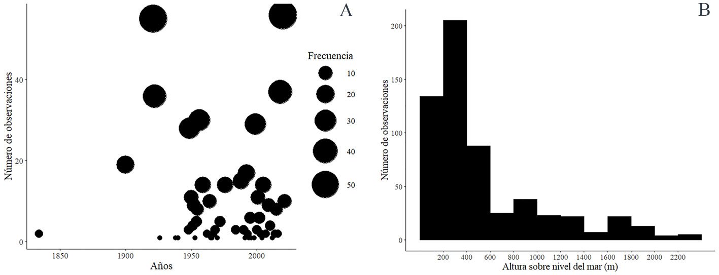
Figura 2. A), Eventualidad de los registros de abejas sin aguijón desde 1984 a 2021; B, número de registros de las abejas sin aguijón en función a la altura sobre el nivel del mar.
Estos registros muestran recolectas que se remontan a 1834 por el naturalista d’Orbigny, posteriormente se observan 2 periodos de particular interés, uno entre los años 1900 y 1970, y otro entre 1980 y 2022 (fig. 2A). Durante el primer periodo, varios naturalistas y recolectores contribuyeron significativamente al conocimiento de la tribu Meliponini en Bolivia. Entre ellos, se destacan Wolfgang Priewasser (1900), Mann (1921 a 1938), Peña (1942 a 1995), Kerr (1949), Kempff. (1962-1968), Bouseman y Lussenhop (1964-1965), Ballard (1967-1968), Walz (1940 – 1955), y Zischka (1950). Para el segundo periodo, sobresalen Brooks (1988), Montaño (1992), Irwin y Parker (1999) y Francois (1999).
En cuanto a la procedencia geográfica de los 616 registros, 273 fueron obtenidos como datos originales, mientras que 272 registros se georreferenciaron con base en las descripciones de los sitios de recolecta en los manuscritos, y adicionalmente, 71 registros tuvieron correcciones en su ubicación geográfica (fig. 3A). De los registros provenientes del GBIF (n = 236), se corrigieron geográficamente 72 debido a discrepancias con la ubicación de las localidades descritas (fig. 3B).
Los datos altitudinales derivados de los registros geográficos muestran que estas abejas se encuentran desde 94 hasta 2,329 m snm (fig. 2B). En este contexto, 66.7% de las especies (n = 80) se localizan en un rango altitudinal desde 94 a 500 m, abarcando el piso ecológico basal que incluye las tierras bajas y parte del subandino. El 27.5% de las especies (n = 33) se encuentra en el piso ecológico basimontano o andino montano situado entre 500 y 1,000 m. Solo 15 especies de abejas sin aguijón han sido registradas por encima de 1,000 m, encontrándose en fondos de valles desde 1,100 hasta 2,400 m, incluyendo especies como Scaptotrigona turusiri en los Yungas, abejas del género Plebeia sp. y Tetragonisca angustula en los valles secos interandinos. Y un caso sorprendente fue el registro de una abeja del género Trigona sp., que se reportó por encima de 4,000 m (altiplano).
La sistematización de los datos posibilita obtener una aproximación de la riqueza de abejas sin aguijón en Bolivia, lo cual se traduce en la identificación de 19 géneros y 121 especies (tablas 1, 2). Es importante señalar que este número podría aumentar hasta 132 especies, siempre y cuando se realice una confirmación taxonómica y biogeográfica de 11, debido a que existen registros próximos a las fronteras de Brasil y Argentina.
En cuanto a la distribución de la riqueza de especies a nivel departamental en Bolivia, se observa que estas abejas están presentes en 7 de los 9 departamentos del país. Destacan los departamentos de La Paz (76 especies), Beni (69 especies), Cochabamba (66 especies) y Santa Cruz (64 especies) como aquellos con el mayor número de especies, seguidos de Chuquisaca (20 especies), Tarija (10 especies) y Pando (9 especies) (tabla 2, fig. 3C). Al considerar los límites de las ecorregiones de Bolivia, se ha determinado que la riqueza de especies está presente en 8 de las 13 ecorregiones, la ecorregión sudoeste de la Amazonía destaca con la mayor riqueza contabilizando 95 especies (tabla 2), seguida de los Yungas (58 especies) y el Cerrado (47 especies). Posteriormente, se encuentran las Sabanas Inundables (27 especies) y el Bosque Seco Chiquitano (25 especies), mientras que las ecorregiones con una menor riqueza incluyen el Gran Chaco (19 especies), el Bosque Tucumano – Boliviano (16 especies), los Bosques Secos Interandinos (16 especies) y el Chaco Serrano (6 especies). Estos hallazgos proporcionan una visión detallada de la diversidad y distribución de las abejas sin aguijón en diferentes regiones de Bolivia.
Discusión
Con base en la revisión bibliográfica que se realizó al trabajo de Camargo y Pedro (2007), para Bolivia se había catalogado un total de 24 géneros. Sin embargo, los cambios introducidos por la reciente publicación de Engel et al. (2023), que presenta una revisión exhaustiva de la clasificación a nivel de género y subgénero de la tribu Meliponini, ha tenido un impacto en la adaptación de la lista, reduciendo el número a 19 géneros. Un ejemplo concreto de estos ajustes se observa en el género Plectoplebeia propuesto por Melo (2016) y con otras especies descritas por Engel (2022), ahora se integran al género Plebeia, debido a la sinonimia y a la presencia de características comunes que comparten, como indican Engel et al. (2023). Asimismo, el género Schwarzula ha sido incluido como subgénero dentro de Scaura, a pesar de que Camargo y Pedro (2002), con base en atributos morfológicos ya había notado fuerte parentesco al identificar sinapomorfias legítimas. No obstante, el análisis filogenético y morfológico realizado por Nogueira (2016) lo distingue como otro género válido (Nogueira, 2023), por lo que se mantiene la discusión sobre su identidad.

Figura 3. Mapa de ubicación de registros geográficos y riqueza de especies de abejas sin aguijón en Bolivia. A), Mapa con datos corregidos, georreferenciados y originales; B) mapa con registros corregidos de GBIF; C), riqueza de especies de abejas sin aguijón obtenido según los municipios en cada departamento; D), a nivel de ecorregiones de Bolivia. Beni (BE), Chuquisaca (CH), Cochabamba (CB), La Paz (LP), Pando (PA), Santa Cruz (SC), Tarija (TA), Oruro (OR) y Potosí (PO).
Otro cambio significativo afecta a los géneros Dolichotrigona, Leurotrigona y Celetrigona, que han sido reclasificados como subgéneros de Trigonisca. Sin embargo, en el caso de Dolichotrigona, ya no se le reconoce como un género valido según Engel et al. (2023). Esto ha llevado a retomar su designación genérica como Trigona propuesto por Wille (1965) y Michener (2013), respaldada por similitudes morfológicas discutidas con Moure, quien dividió estos grupos (Wille, 1979). Plebia intermedia, nombre propuesto para Bolivia por Wille (1960) y citado en el catálogo de abejas de la región neotropical como Plectoplebeia nigrifacies (Camargo y Pedro, 2007), ha experimentado un cambio a Plebeia (Plebeia) nigrifacies. Este cambio se debe a que Melo (2016) la considera una sinonimia y Engel et al. (2023) no la reconoce como especie válida. Estos ajustes en la clasificación taxonómica reflejan la dinámica evolutiva del conocimiento y la importancia de las actualizaciones regulares en la nomenclatura de las abejas sin aguijón en Bolivia.
Tabla 1
Lista de especies de abejas sin aguijón (Meliponini) consensuada a partir de los diferentes registros que se han revisado como el Catálogo de abejas de Moure – A.B.E.L.H.A. (A.B.E.L.H.A., 2016; Camargo, Pedro, et al., 2013; Camargo y Pedro, 2007), World Bee Diversity (Ascher y Pickering, 2020), GBIF, 2022, la lista de especies de abejas nativas de Lisperger (2015) (Townsend, 2016) y las publicaciones revisadas. Registros de especies que están en Bolivia por su proximidad (P). Los valores en negrita corresponden a la sumatoria total del número de especies según el género y las fuentes consultadas.
| Taxones | CAM – (2007-2013) | A.B.E.L.H.A. (2022) | WBA (2020) | GBIF (2022) | Revisión Pub. | Subtotal | Total |
| Subtribu Meliponina Lepeletier | |||||||
| Infratribu Meliponitae Lepeletier | |||||||
| Grupos de Género Paratrigona | |||||||
| Género Paratrigona Schwarz, 1938 | 7 | 7 | 7 | 4 | 7 | 8 | 8 |
| Paratrigona (Paratrigona) glabella Camargo et Moure, 1994 | 1 | 1 | 1 | 1 | 1 | ||
| Paratrigona (Paratrigona) guigliae Moure, 1960 | 1 | 1 | 1 | 1 | 1 | 1 | |
| Paratrigona (Paratrigona) lineata (Lepeletier, 1836) | 1 | 1 | 1 | 1 | 1 | 1 | |
| Paratrigona (Paratrigona) nuda (Schwarz, 1943) | 1 | 1 | 1 | 1 | 1 | 1 | 1 |
| Paratrigona (Paratrigona) onorei Camargo et Moure, 1994 | 1 | 1 | 1 | 1 | 1 | 1 | |
| Paratrigona (Paratrigona) pacifica (Schwarz, 1943) | 1 | 1 | 1 | 1 | 1 | 1 | 1 |
| Paratrigona (Paratrigona) prosopiformis (Gribodo, 1893) | 1 | 1 | 1 | 1 | 1 | 1 | 1 |
| Paratrigona (Paratrigona) subnuda Moure, 1947 | 1 | 1 | 1 | 1 | |||
| Género Nogueirapis Moure, 1953 | 1 | 1 | 1 | ||||
| Nogueirapis butteli (Friese, 1900)? | 1 | 1 | 1 | ||||
| Género Partamona Schwarz, 1939 | 9 | 9 | 9 | 8 | 8 | 9 | 10 |
| Partamona ailyae Camargo, 1980 | 1 | 1 | 1 | 1 | 1 | 1 | 1 |
| Paratrigona (Paratrigona) batesi Pedro et Camargo, 2003p | 1 | 1 | |||||
| Partamona combinata Pedro et Camargo, 2003 | 1 | 1 | 1 | 1 | 1 | 1 | 1 |
| Partamona epiphytophila Pedro et Camargo, 2003 | 1 | 1 | 1 | 1 | 1 | 1 | 1 |
| Partamona mulata Moure, in Camargo, 1980 | 1 | 1 | 1 | 1 | 1 | 1 | 1 |
| Partamona nhambiquara Pedro et Camargo, 2003 | 1 | 1 | 1 | 1 | 1 | ||
| Partamona subtilis Pedro et Camargo, 2003 | 1 | 1 | 1 | 1 | 1 | 1 | 1 |
| Partamona testacea (Klug, 1807) | 1 | 1 | 1 | 1 | 1 | 1 | 1 |
| Partamona vicina Camargo, 1980 | 1 | 1 | 1 | 1 | 1 | 1 | 1 |
| Partamona yungarum Pedro et Camargo, 2003 | 1 | 1 | 1 | 1 | 1 | 1 | 1 |
| Grupos de Género Trigona | |||||||
| Género Oxytrigona Cockerell, 1917 | 2 | 2 | 2 | 4 | 4 | 4 | 4 |
| Oxytrigona mulfordi (Schwarz, 1948) | 1 | 1 | 1 | 1 | 1 | 1 | 1 |
| Oxytrigona flaveola (Friese, 1900) | 1 | 1 | 1 | 1 | |||
| Oxytrigona obscura (Friese, 1900) | 1 | 1 | 1 | 1 | 1 | 1 | 1 |
| Oxytrigona tataira (Smith, 1863) | 1 | 1 | 1 | 1 | |||
| Genero Scaptotrigona Moure, 1942 | 6 | 5 | 5 | 2 | 13 | 13 | 14 |
| Subgénero Baryorygma Engel | |||||||
| Scaptotrigona (Baryorygma) bipunctata (Lepeletier, 1836) | 1 | 1 | 1 | 1 | 1 | 1 | |
| Scaptotrigona (Baryorygma) fimbriata Engel, 2022 | 1 | 1 | 1 |
| Tabla 1. Continúa | |||||||
| Taxones | CAM – (2007-2013) | A.B.E.L.H.A. (2022) | WBA (2020) | GBIF (2022) | Revisión Pub. | Subtotal | Total |
| Scaptotrigona (Baryorygma) tricolorata Camargo, 1988 | 1 | 1 | 1 | 1 | 1 | 1 | |
| Subgénero Eoscaptotrigona Engel | |||||||
| Scaptotrigona (Eoscaptotrigona) polysticta Moure, 1950 | 1 | 1 | 1 | 1 | 1 | 1 | 1 |
| Subgénero Gymnotrigona Engel | |||||||
| Scaptotrigona (Gymnotrigona) depilis (Moure, 1942) | 1 | 1 | 1 | 1 | 1 | 1 | 1 |
| Scaptotrigona (Gymnotrigona) jujuyensis (Schrottky, 1911)P | 1 | ||||||
| Scaptotrigona (Gymnotrigona) nuda Engel, 2022 | 1 | 1 | 1 | ||||
| Subgénero Scaptotrigona Moure | |||||||
| Scaptotrigona (Scaptotrigona) grueteri Engel, 2022 | 1 | 1 | 1 | ||||
| Scaptotrigona (Scaptotrigona) nigrohirta Nogueira et Santos-Silva 2022 | 1 | 1 | 1 | ||||
| Scaptotrigona (Scaptotrigona) postica (Latreille, 1807) | 1 | 1 | 1 | 1 | 1 | 1 | |
| Scaptotrigona (Scaptotrigona) semiflava Engel, 2022 | 1 | 1 | 1 | ||||
| Scaptotrigona (Scaptotrigona) turusiri (Janvier, 1955) | 1 | 1 | 1 | 1 | |||
| Scaptotrigona (Scaptotrigona) xanthotricha Moure, 1950 | 1 | 1 | 1 | ||||
| Scaptotrigona (Scaptotrigona) yungasensis Engel, 2022 | 1 | 1 | 1 | ||||
| Género Geotrigona Moure, 1943 | 5 | 5 | 5 | 3 | 5 | 6 | 5 |
| Subgenero Chthonotrigona Engel | |||||||
| Geotrigona (Chthonotrigona) fulvohirta (Friese, 1900) | 1 | 1 | 1 | 1 | 1 | 1 | 1 |
| Subgénero Geotrigona Engel | |||||||
| Geotrigona (Geotrigona) argentina Camargo et Moure, 1996 | 1 | 1 | 1 | 1 | 1 | 1 | |
| Geotrigona (Geotrigona) fulvatra Camargo et Moure, 1996 | 1 | 1 | 1 | 1 | 1 | 1 | 1 |
| Geotrigona (Geotrigona) mattogrossensis (Ducke, 1925) | 1 | 1 | 1 | 1 | 1 | 1 | |
| Geotrigona (Geotrigona) mombuca (Smith, 1863) | 1 | 1 | 1 | ||||
| Geotrigona (Geotrigona) tellurica Camargo et Moure, 1996 | 1 | 1 | 1 | 1 | 1 | 1 | 1 |
| Género Ptilotrigona Moure, 1951 | 1 | 1 | 1 | 1 | 1 | 1 | 1 |
| Ptilotrigona (Ptilotrigona) lurida (Smith, 1854) | 1 | 1 | 1 | 1 | 1 | 1 | 1 |
| Género Tetragona Lepeletier et Serville, 1828 | 3 | 3 | 3 | 2 | 3 | 3 | 3 |
| Tetragona clavipes (Fabricius, 1804) | 1 | 1 | 1 | 1 | 1 | 1 | 1 |
| Tetragona goettei (Friese, 1900) | 1 | 1 | 1 | 1 | 1 | 1 | 1 |
| Tetragona truncata Moure, 1971 | 1 | 1 | 1 | 1 | 1 | 1 | |
| Género Trigona Jurine, 1807 | 16 | 16 | 16 | 23 | 16 | 19 | 22 |
| Subgénero Aphaneura Gray | |||||||
| Trigona (Aphaneura) chanchamayoensis Schwarz, 1948 | 1 | 1 | 1 | 1 | 1 | 1 | 1 |
| Trigona (Aphaneura) pallens (Fabricius, 1798) | 1 | 1 | 1 | ||||
| Trigona (Aphaneura) williana Friese, 1900 | 1 | 1 | 1 | 1 | 1 | 1 | 1 |
| Subgénero Aphaneuropsis Engel | |||||||
| Trigona (Aphaneuropsis) cilipes (Fabricius, 1804) | 1 | 1 | 1 | 1 | 1 | 1 | 1 |
| Trigona (Aphaneuropsis) lacteipennis Friese, 1900 | 1 | 1 | 1 | 1 | 1 | 1 | |
| Subgénero Dichrotrigona Engel | |||||||
| Trigona (Dichrotrigona) dimidiata Smith, 1854 | 1 | 1 | 1 | 1 | 1 | 1 | 1 |
| Subgénero Koilotrigona Engel | |||||||
| Trigona (Koilotrigona) fulviventris Guérin, 1844 | 1 | 1 | 1 | ||||
| Trigona (Koilotrigona) guianae Cockerell, 1910 | 1 | 1 | 1 | 1 | 1 | 1 | 1 |
| Subgénero Ktinotrofia Engel | |||||||
| Trigona (Ktinotrofia) albipennis Almeida, 1995 | 1 | 1 | 1 | 1 | 1 | 1 | |
| Trigona (Ktinotrofia) fuscipennis Friese, 1900 | 1 | 1 | 1 | ||||
| Subgénero Necrotrigona Engel | |||||||
| Trigona (Necrotrigona) crassipes (Fabricius, 1793) | 1 | 1 | 1 | 1 | 1 | 1 | 1 |
| Trigona (Necrotrigona) hypogea Silvestri, 1902 | 1 | 1 | 1 | 1 | 1 | 1 | 1 |
| Subgénero Nostotrigona Engel | |||||||
| Trigona (Nostotrigona) juvenili Ribeiro, 2023p | 1 | 1 | |||||
| Trigona (Nostotrigona) recursa Smith, 1863 | 1 | 1 | 1 | 1 | 1 | 1 | 1 |
| Subgénero Trigona Jurine | |||||||
| Trigona (Trigona) amalthea (Olivier, 1789) | 1 | 1 | 1 | 1 | 1 | 1 | 1 |
| Trigona (Trigona) amazonensis (Ducke, 1916) | 1 | 1 | 1 | 1 | 1 | 1 | 1 |
| Trigona (Trigona) branneri Cockerell, 1912 | 1 | 1 | 1 | 1 | 1 | 1 | 1 |
| Trigona (Trigona) corvina Cockerell, 1913 | 1 | 1 | 1 | ||||
| Trigona (Trigona) dallatorreana Friese, 1900 | 1 | 1 | 1 | 1 | 1 | 1 | 1 |
| Trigona (Trigona) hyalinata (Lepeletier, 1836) | 1 | 1 | 1 | 1 | 1 | 1 | 1 |
| Trigona (Trigona) silvestriana (Vachal, 1908) | 1 | 1 | 1 | 1 | |||
| Trigona (Trigona) truculenta Almeida, 1984 | 1 | 1 | 1 | 1 | 1 | 1 | |
| Género Cephalotrigona Schwarz, 1940 | 2 | 2 | 2 | 2B | 2 | 2 | 2 |
| Cephalotrigona capitata (Smith, 1854) | 1 | 1 | 1 | 1 | 1 | 1 | 1 |
| Cephalotrigona femorata (Smith, 1854) | 1 | 1 | 1 | 1 | 1 | 1 | |
| Grupos de Género Plebeia | |||||||
| Género Tetragonisca Moure, 1946 | 3 | 2 | 2 | 3 | 3 | 3 | 3 |
| Tetragonisca angustula (Latreille, 1811) | 1 | 1 | 1 | 1 | 1 | ||
| Tetragonisca fiebrigi (Schwarz, 1938) | 1 | 1 | 1 | 1 | 1 | 1 | 1 |
| Tetragonisca weyrauchi (Schwarz, 1943) | 1 | 1 | 1 | 1 | 1 | 1 | 1 |
| Género Frieseomelitta Ihering, 1912 | 2 | 3 | 2 | 4 | 2 | 3 | 3 |
| Frieseomelitta silvestrii (Friese, 1902) | 1 | 1 | 1 | 1 | 1 | 1 | 1 |
| Frieseomelitta flavicornis (Fabricius, 1798) | 1 | 1 | 1 | ||||
| Frieseomelitta trichocerata Moure, 1990 | 1 | 1 | 1 | ||||
| Frieseomelitta varia (Lepeletier, 1836) | 1 | 1 | 1 | 1 | 1 | 1 | 1 |
| Género Duckeola Moure, 1944 | 1 | 1 | 1 | 1 | 1 | 1 | 1 |
| Duckeola ghilianii (Spinola, 1853) | 1 | 1 | 1 | 1 | 1 | 1 | 1 |
| Género Plebeia Schwarz, 1938 | 5 | 5 | 5 | 3 | 9 | 9 | 10 |
| Subgénero Nanoplebeia Engel | |||||||
| Plebeia (Nanoplebeia) asthenes Engel, 2021 | 1 | 1 | 1 | ||||
| Plebeia (Nanoplebeia) minima (Gribodo, 1893) | 1 | 1 | 1 | 1 | 1 | 1 | |
| Subgénero Plebeia Schwarz, s.str. | |||||||
| Plebeia (Plebeia) alvarengai Moure, 1994 | 1 | 1 | 1 | 1 | |||
| Plebeia (Plebeia) droryana (Friese, 1900) | 1 | 1 | 1 | 1 | 1 | 1 | 1 |
| Plebeia (Plebeia) kerri Moure, 1950 | 1 | 1 | 1 | 1 | 1 | 1 | 1 |
| Plebeia (Plebeia) mosquito (Smith, 1863)? | 1 | 1 | 1 | ||||
| Plebeia (Plebeia) mansita Alvarez et Rasmussen, 2021P | 1 | 1 | |||||
| Plebeia (Plebeia) nigrifacies (Friese, 1900) | 1 | 1 | 1 | 1 | 1 | 1 | |
| Plebeia (Plebeia) peruvicola Moure, 1994 | 1 | 1 | 1 | ||||
| Plebeia (Plebeia) remota (Holmberg, 1903) | 1 | 1 | 1 | 1 | 1 | 1 | |
| Género Lestrimelitta Friese, 1903 | 1 | 1 | 1 | 1 | 3 | 3 | 3 |
| Subgénero Hyrolestris Engel | |||||||
| Lestrimelitta (Hyrolestris) rufipes (Friese, 1903) | 1 | 1 | 1 | 1 | |||
| Subgénero Lestrimelitta Friese, s.str. | |||||||
| Lestrimelitta (Lestrimelitta) rufa (Friese, 1903) | 1 | 1 | 1 | 1 | 1 | 1 | |
| Género Nannotrigona Cockerell, 1922 | 2 | 2 | 2 | 3 | 2 | 2 | 3 |
| Subgénero Lispotrigona González et Engel | |||||||
| Nannotrigona (Lispotrigona) schultzei (Friese, 1901) | 1 | 1 | 1 | 1 | 1 | 1 | 1 |
| Subgénero Nannotrigona Cockerell, s.str. | |||||||
| Nannotrigona (Nannotrigona) melanocera (Schwarz, 1938) | 1 | 1 | 1 | 1 | 1 | 1 | 1 |
| Nannotrigona (Nannotrigona) testaceicornis (Lepeletier, 1836)? | 1 | 1 | |||||
| Género Scaura Schwarz, 1938 | 2 | 3 | 3 | 4 | 4 | 4 | |
| Subgénero Scaura Schwarz, s.str. | |||||||
| Scaura (Scaura) latitarsis (Friese, 1900) | 1 | 1 | 1 | 1 | 1 | 1 | |
| Scaura (Scaura) longula (Lepeletier, 1836) | 1 | 1 | 1 | 1 | 1 | 1 | |
| Subgénero Scauracea Engel | |||||||
| Scaura (Scauracea) amazonica Nogueira, Oliveira e Oliveira, 2016 | 1 | 1 | 1 | 1 | 1 | ||
| Subgénero Schwarzula Moure | |||||||
| Scaura (Schwarzula) timida (Silvestri, 1902) | 1 | 1 | 1 | 1 | 1 | 1 | 1 |
| Grupos de Género Melipona | |||||||
| Género Melipona Illiger, 1806 | 15 | 15 | 15 | 17 | 17 | 18 | 21 |
| Subgénero Eomelipona Moure | |||||||
| Melipona (Eomelipona) amazonica Schulz, 1905P | 1 | 1 | |||||
| Melipona (Eomelipona) tumupasae Schwarz, 1932 | 1 | 1 | 1 | 1 | 1 | 1 | 1 |
| Subgénero Melikerria Moure | |||||||
| Melipona (Melikerria) fasciculata Smith, 1854 | 1 | 1 | 1 | ||||
| Melipona (Melikerria) grandis Guérin, 1844 | 1 | 1 | 1 | 1 | 1 | 1 | 1 |
| Melipona (Melikerria) quinquefasciata Lepeletier, 1836 | 1 | 1 | 1 | 1 | 1 | 1 | |
| Subgénero Melipona Illiger, s.str. | |||||||
| Melipona (Melipona) baeri Vachal, 1904 | 1 | 1 | 1 | 1 | 1 | 1 | 1 |
| Melipona (Melipona) fuscata Lepeletier, 1836 | 1 | 1 | 1 | 1 | |||
| Melipona (Melipona) lunulata Friese, 1900 | 1 | 1 | 1 | 1 | 1 | 1 | 1 |
| Melipona (Melipona) orbignyi (Guérin, 1844) | 1 | 1 | 1 | 1 | 1 | 1 | 1 |
| Subgénero Michmelia Moure | |||||||
| Melipona (Michmelia) boliviana Schwarz, 1932 | 1 | 1 | 1 | 1 | 1 | 1 | 1 |
| Melipona (Michmelia) brachychaeta Moure, 1950 | 1 | 1 | 1 | 1 | 1 | 1 | 1 |
| Melipona (Michmelia) crinita Moure et Kerr, 1950 | 1 | 1 | 1 | 1 | 1 | 1 | |
| Melipona (Michmelia) eburnea Friese, 1900 | 1 | 1 | 1 | 1 | 1 | 1 | 1 |
| Melipona (Michmelia) flavolineata Friese, 1900p | 1 | 1 | |||||
| Melipona (Michmelia) illota Cockerell, 1919 | 1 | 1 | 1 | 1 | 1 | 1 | |
| Melipona (Michmelia) nebulosa Camargo, 1988 | 1 | 1 | 1 | 1 | 1 | 1 | |
| Melipona (Michmelia) rufescens Friese, 1900 | 1 | 1 | 1 | 1 | 1 | 1 | 1 |
| Melipona (Michmelia) rufiventris Lepeletier, 1836 | 1 | 1 | 1 | 1 | |||
| Melipona (Michmelia) rufiventris xantina | 1 | ? | |||||
| Melipona (Michmelia) seminigra abunensis Cockerell, 1912 | 1 | 1 | 1 | 1 | 1 | 1 | 1 |
| Subgénero Mouremelia Engel | |||||||
| Melipona (Mouremelia) fuliginosa Lepeletier, 1836 | 1 | 1 | 1 | 1 | 1 | 1 | 1 |
| Melipona (Mouremelia) titania (Gribodo, 1893)P | 1 | 1 | |||||
| Infratribu Trigoniscitae Engel Grupos de Género Trigonisca | |||||||
| Género Trigonisca Moure, 1950 | 5 | 4 | 4 | 3 | 8 | 9 | 13 |
| Subgénero Celetrigona Moure, 1950 | |||||||
| Trigonisca (Celetrigona) longicornis (Friese, 1903) | 1 | 1 | 1 | 1 | 1 | 1 | |
| Trigonisca (Celetrigona) hirsuticornis Camargo et Pedro, 2009p | 1 | 1 | 1 | ||||
| Subgénero Leurotrigona Moure, 1950 | |||||||
| Trigonisca (Leurotrigona) gracilis Pedro et Camargo, 2009p | 1 | ||||||
| Trigonisca (Leurotrigona) muelleri (Friese, 1900) | 1 | 1 | 1 | 1 | 1 | 1 | |
| Subgénero Trigonisca Moure, 1950 | |||||||
| Trigonisca (Trigonisca) browni Camargo et Pedro, 2005 | 1 | 1 | 1 | 1 | 1 | 1 | 1 |
| Trigonisca (Trigonisca) duckei (Friese, 1900) | 1 | 1 | 1 | 1 | 1 | 1 | |
| Trigonisca (Trigonisca) intermedia Moure, 1990 | 1 | 1 | 1 | ||||
| Trigonisca (Trigonisca) longitarsis (Ducke, 1916) | 1 | 1 | 1 | 1 | |||
| Trigonisca (Trigonisca) mendersoni Camargo et Pedro, 2005P | 1 | 1 | |||||
| Trigonisca (Trigonisca) pediculana (Fabricius, 1804) | 1 | 1 | 1 | 1 | |||
| Trigonisca (Trigonisca) rondoni Camargo et Pedro, 2005P | 1 | 1 | |||||
| Trigonisca (Trigonisca) sachamiski Alvarez et Lucia, 2018P | 1 | ||||||
| Trigonisca (Trigonisca) vitrifrons Albuquerque et Camargo, 2007 | 1 | 1 | 1 | ||||
| Géneros | 21 | 23 | 23 | 20 | 24 | 19 | 19 |
| Especies | 88 | 86 | 86 | 88 | 113 | 118 | 133 |
Tabla 2
Lista de especies registradas par Bolivia, con información de presencia a nivel de los límites departamentales y ecorregiones, y el intervalo de tiempo de los registros. Departamentos de Bolivia: Beni (BE), Chuquisaca (CH), Cochabamba (CB), La Paz (LP), Pando (PA), Santa Cruz (SC) y Tarija (TA). Ecorregiones: Bosque Seco Chiquitano (BSChi), Bosque Tucumano – Boliviano (BTBo), Bosques Secos Interandinos (BSIn), Cerrado (Cer), Chaco Serrano (ChaSe), Gran Chaco (GCha), Sabanas Inundables (SaIn), Sudoeste de la Amazonía (SAmz), Yungas (Yun).
| Lista de taxones | Dep | Eco | Años | Referencias |
| Género Paratrigona Schwarz, 1938 | ||||
| Paratrigona glabella Camargo y Moure, 1994 | CH, CB, LP SC, TA | BSChi, BTBo, BSIn, ChaSe GCha, SAmz, Yun | 1952-2020 | Camargo y Moure, 1994; GBIF.org, 2022; Oliveira et al., 2020 |
| Paratrigona guigliae Moure, 1960 | LP | Yun | ~1950 | Camargo y Moure, 1994 |
| Paratrigona lineata (Lepeletier, 1836) | CH, CB, SC | BSChi, Cer, BTBo, BSIn, Cer, Yun | 1951-2015 | Camargo y Moure, 1994; GBIF.org, 2022; Oliveira et al., 2020 |
| Paratrigona nuda (Schwarz, 1943) | LP | SAmz, Yun | 1950-1956 | Camargo y Moure, 1994; GBIF.org, 2022; Oliveira et al., 2020 |
| Paratrigona onorei Camargo y Moure, 1994 | CB | Yun | 1950 | Camargo y Moure, 1994 |
| Paratrigona pacifica (Schwarz, 1943) | CB, LP | SAmz, Yun | 1949-2001 | Camargo y Moure, 1994; GBIF.org, 2022 |
| Paratrigona prosopiformis (Gribodo, 1893) | CB, LP, SC | SAmz, Yun | 1948-2001 | Camargo y Moure, 1994; GBIF.org, 2022 |
| Paratrigona subnuda Moure, 1947 | CB | SAmz | WBD, 2020 | |
Género Nogueirapis Moure, 1953 | ||||
| Nogueirapis butteli (Friese, 1900) | CB | SAmz | 1900 | GBIF.org, 2022; Wille, 1962 |
Género Partamona Schwarz, 1939 | ||||
| Paratrigona ailyae Camargo, 1980 | BE, CB | SAmz, SaIn, Yun | 1948-2018 | GBIF.org, 2022; Stearman et al., 2008; Townsend et al., 2021 |
| Partamona combinata Pedro y Camargo, 2003 | BE, CB, LP, SC | SAmz, SaIn, Yun | 1922-1990 | GBIF.org, 2022; Pedro y Camargo, 2003 |
| Partamona epiphytophila Pedro y Camargo, 2003 | BE, CB, LP, PA, SC | BSIn, Cer, SAmz, Yun | 1921-2000 | GBIF.org, 2022; Pedro y Camargo, 2003 |
| Partamona mulata Moure, in Camargo, 1980 | BE, SC | GCha, SILM | 1952-1992 | GBIF.org, 2022; Pedro y Camargo, 2003 |
| Partamona nhambiquara Pedro y Camargo, 2003 | BE | SAmz | 1922 | GBIF.org, 2022 |
| Partamona subtilis Pedro y Camargo, 2003 | BE | SAmz | 1956 | GBIF.org, 2022; Pedro y Camargo, 2003 |
| Partamona testacea (Klug, 1807) | BE, LP | SAmz | 1921-1956 | GBIF.org, 2022; Pedro y Camargo, 2003 |
| Partamona vicina Camargo, 1980 | LP, SC | Cer, SAmz | 1959-2018 | GBIF.org, 2022; Pedro y Camargo, 2003; Townsend et al., 2021 |
| Partamona yungarum Pedro y Camargo, 2003 | LP, CB | BSIn | 1948-1955 | GBIF.org, 2022; Pedro y Camargo, 2003 |
| Tabla 2. Continúa | ||||
| Lista de taxones | Dep | Eco | Años | Referencias |
| Género Oxytrigona Cockerell, 1917 | ||||
| Oxytrigona flaveola (Friese, 1900) | BE, LP, SC | Cer, GCha, SAmz, Yun | 1921-2020 | GBIF.org, 2022; Schwarz, 1948 |
| Oxytrigona mulfordi (Schwarz, 1948) | BE, LP, SC | SAmz | 1921-1956 | GBIF.org, 2022; Schwarz, 1948 |
| Oxytrigona obscura (Friese, 1900) | BE, CB, LP PA, SC | GCha, SAmz, Yun | 1921-2020 | GBIF.org, 2022; Schwarz, 1948 |
| Oxytrigona tataira (Smith, 1863) | BE, LP SC, TA | GCha, SAmz, Yun | 1921-2018 | Camargo, 1988; Clemente y Lahore, 2010; GBIF.org, 2022; Schwarz, 1948; Townsend et al., 2021 |
Género Scaptotrigona Moure, 1942 | ||||
| Scaptotrigona bipunctata (Lepeletier, 1836) | CH, LP | SaIn, SAmz, Yun | 1964 – 2020 | Camargo, 1988; Tejada, 2006; este trabajo |
| Scaptotrigona fimbriata Engel, 2022 | BE, SC | BSChi, SAmz | 1988 – 2002 | Engel, 2022 |
| Scaptotrigona tricolorata Camargo, 1988 | CB | SAmz | 1949 | Engel, 2022; GBIF.org, 2022 |
| Scaptotrigona polysticta Moure, 1950 | BE, CH, CB, LP, SC | BSChi, Cer, SaIn, SAmz, Yun | 1949 – 2020 | FCBC, 2021; Ferrufino, 2013; GBIF.org, 2022; Montaño, 1996; Moure, 1950; Tejada, 2006; Townsend et al., 2021; este trabajo |
| Scaptotrigona depilis (Moure, 1942) | BE, CB, LP, SC, TA | BSChi, Cer, GCha, SaIn, SAmz, Yun | 1949 – 2020 | Clemente y Lahore, 2010; Ferrufino, 2013; GBIF.org, 2022; Moure, 1950; Tejada, 2006; Townsend et al., 2021; este trabajo |
| Scaptotrigona nuda Engel, 2022 | BE | SAmz | 1988 | Engel, 2022 |
| Scaptotrigona grueteri Engel, 2022 | LP | Yun | 1955-1992 | Engel, 2022 |
| Scaptotrigona nigrohirta Nogueira y Santos-Silva, 2022 | CB | SAmz | 2007 | Stearman et al., 2008 |
| Scaptotrigona postica (Latreille, 1807) | BE, SC | GCha, SaIn | 1992-2002 | Martínez y Cuéllar, 2004; Montaño, 1996 |
| Scaptotrigona semiflava Engel, 2022 | SC | BSChi | 1951 | Engel, 2022 |
| Scaptotrigona turusiri (Janvier, 1955) | CB | Engel, 2022 | ||
| Scaptotrigona xanthotricha Moure, 1950 | CB, LP, SC | BSChi, SAmz, Yun | 2020 | Camargo, 1988; Ferrufino, 2013; este trabajo |
| Scaptotrigona yungasensis Engel, 2022 | BE, CB, LP | SaIn, SAmz, Yun | 1955-1966 | Engel, 2022 |
Género Geotrigona Moure, 1943 | ||||
| Geotrigona fulvohirta (Friese, 1900) | BE, LP | Cer, SAmz | 1922 -2005 | Camargo y Moure, 1996; GBIF.org, 2022; Tejada, 2006 |
| Geotrigona argentina Camargo y Moure, 1996 | CH, SC, TA | Cer, BTBo, GCha | 1949-2015 | Camargo y Moure, 1996; Clemente y Lahore, 2010 |
| Geotrigona fulvatra Camargo y Moure, 1996 | BE, LP | Cer, SAmz | 1922 -1956 | Camargo y Moure, 1996; GBIF.org, 2022 |
| Geotrigona mattogrossensis (Ducke, 1925) | SC | Cer | 1951 | Camargo y Moure, 1996; GBIF.org, 2022 |
| Geotrigona tellurica Camargo y Moure, 1996 | CB, LP | Cer | 1921-1956 | Camargo y Moure, 1996; GBIF.org, 2022 |
| Geotrigona mombuca (Smith, 1863) | CH, SC | Cer | 1949 -2015 | Moure, 1950 |
Género Ptilotrigona Moure, 1951 | ||||
| Ptilotrigona lurida (Smith, 1854) | BE, LP | SaIn, Yun | 1964 – 2020 | GBIF.org, 2022; Montaño, 1996 |
Género Tetragona Lepeletier y Serville, 1828 | ||||
| Tetragona clavipes (Fabricius, 1804) | CB, CH, LP SC | BSChi, BTBo, Cer, SAmz | 2020-2018 | FCBC, 2021; Nogueira et al., 2022; Stearman et al., 2008; Townsend et al., 2021; este trabajo |
| Tetragona gottei (Friese, 1900) | BE, CB, LP, SC | BSChi, SaIn, SAmz, Yun | 2020-2018 | Camargo, 1988; FCBC, 2021; Stearman et al., 2008; Townsend et al., 2021 |
| Tetragona truncata Moure, 1971 | LP, PA | SAmz, Yun | ? | A.B.E.L.H.A., 2016; Camargo, 1988 |
Género Trigona Jurine, 1807 | ||||
| Trigona chanchamayoensis Schwarz, 1948 | BE, CB, LP, SC | BSChi, Cer, SaIn, SAmz, Yun | 1956-2021 | Camargo, 1988; FCBC, 2021; GBIF.org, 2022; Montaño, 1996; Moure, 1950; Schwarz, 1948; Townsend et al., 2021; este trabajo |
| Trigona pallens (Fabricius, 1798) | BE, CB, SC | Cer, SaIn, SAmz | 1956-1999 | GBIF.org, 2022 |
| Trigona williana Friese, 1900 | BE, CB | SAmz | 1900-1964 | GBIF.org, 2022; Schwarz, 1948 |
| Trigona cilipes (Fabricius, 1804) | BE, CB, LP, SC | BSChi, Cer, SaIn, SAmz, Yun | 1951-1962 | Almeida, 1992; Camargo, 1988; Kempf-Mercado, 1968; Stearman et al., 2008 |
| Trigona lacteipennis Friese, 1900 | BE, LP | SAmz | 1922-1976 | A.B.E.L.H.A., 2016; GBIF.org, 2022 |
| Trigona dimidiata Smith, 1854 | BE, CB, LP | SAmz, Yun | 1900-2020 | GBIF.org, 2022; Schwarz, 1948; este trabajo |
| Trigona fulviventris Guérin, 1844 | BE, CB | SAmz, Yun | 1956-1999 | GBIF.org, 2022 |
| Trigona guianae Cockerell, 1910 | BE, CB, LP, SC | BSChi, SaIn, SAmz | 1921-1999 | GBIF.org, 2022; Schwarz, 1948 |
| Trigona albipennis Almeida, 1995 | CB, PA | SAmz | 1949-1999 | A.B.E.L.H.A., 2016; GBIF.org, 2022; Ribeiro, 2021 |
| Trigona fuscipennis Friese, 1900 | BE, CB, SC | BSChi, SaIn, SAmz | 1992-2020 | FCBC, 2021; Montaño, 1996; Stearman et al., 2008; Townsend et al., 2021 |
| Trigona crassipes (Fabricius, 1793) | LP | SAmz, Yun | 1921-1956 | A.B.E.L.H.A., 2016; Camargo, 1988; GBIF.org, 2022; Schwarz, 1948 |
| Trigona hypogea Silvestri, 1902 | BE, CB, PA, SC | SAmz | 1921-2018 | GBIF.org, 2022; Schwarz, 1948; Stearman et al., 2008; Townsend et al., 2021 |
| Trigona recursa Smith, 1863 | BE, LP, SC | Cer, SAmz, Yun | 1921-2018 | GBIF.org, 2022; Moure, 1950; Schwarz, 1948; Townsend et al., 2021 |
| Trigona amalthea (Olivier, 1789) | BE, CB, LP, PA, SC | BTBo, SAmz | 1900-1956 | GBIF.org, 2022; Schwarz, 1948 |
| Trigona amazonensis (Ducke, 1916) | BE, CB, LP, PA | Cer, SAmz, Yun | 1900-1956 | Camargo, 1988; GBIF.org, 2022; Tejada, 2006 |
| Trigona branneri Cockerell, 1912 | BE, CB, LP, SC | BSChi, Cer, SaIn, SAmz, Yun | 1956-2020 | Camargo, 1988; FCBC, 2021; GBIF.org, 2022; Montaño, 1996; Townsend et al., 2021 |
| Trigona corvina Cockerell, 1913 | BE, SC | Cer, SAmz | 1956-1959 | GBIF.org, 2022 |
| Trigona dallatorreana Friese, 1900 | BE, CB, LP | SAmz, Yun | 1900-2020 | Camargo, 1988; GBIF.org, 2022; Schwarz, 1948; este trabajo |
| Trigona hyalinata (Lepeletier, 1836) | BE, LP | SAmz | 1922-1964 | GBIF.org, 2022; Schwarz, 1948 |
| Trigona silvestriana (Vachal, 1908) | CB, LP, SC | BSChi, Cer, SAmz, Yun | 1900-2018 | FCBC, 2021; GBIF.org, 2022; Stearman et al., 2008; Townsend et al., 2021 |
| Trigona truculenta Almeida, 1984 | BE, CB, LP | SAmz | 1956-1991 | A.B.E.L.H.A., 2016; GBIF.org, 2022 |
Género Cephalotrigona Schwarz, 1940 | ||||
| Cephalotrigona capitata (Smith, 1854) | BE, CB, LP, SC, TA | SAmz, Yun, Cer, SaIn, BSChi, GCha | 1900-2021 | FCBC, 2021; GBIF.org, 2022; Kempf-Mercado, 1968; Schwarz, 1948; Tejada, 2006; Townsend et al., 2021 |
| Cephalotrigona femorata (Smith, 1854) | BE, LP | SAmz | 1922 | Schwarz, 1948 |
Género Tetragonisca Moure, 1946 | ||||
| Tetragonisca angustula (Latreille, 1811) | CB, CH, LP SC, TA | BSChi, BTBo, ChaSe, GCha, SAmz, Yun | 1956-2020 | Clemente y Lahore, 2010; Copa-Alvaro, 2004; Flores, 2016; GBIF.org, 2022; Martínez y Cuéllar, 2004; Stearman et al., 2008; Tejada, 2006; este trabajo |
| Tetragonisca fiebrigi (Schwarz, 1938) | SC, CH | BSChi, BTBo, Cer | 1949-2020 | Ferrufino, 2013; Moure, 1950; Townsend et al., 2021; este trabajo |
| Tetragonisca weyrauchi (Schwarz, 1943) | SC, CH | BSChi, BTBo, Cer | 1921-2020 | GBIF.org, 2022; Tejada, 2006; este trabajo |
Género Frieseomelitta Ihering, 1912 | ||||
| Frieseomelitta flavicornis (Fabricius, 1798) | LP | SAmz | 1990 | GBIF.org, 2022 |
| Frieseomelitta silvestrii (Friese, 1902) | SC | Cer | 1949-1959 | GBIF.org, 2022; Moure, 1950 |
| Frieseomelitta trichocerata Moure, 1990 | BE, CB, LP | SAmz, BSIn | ~1950 -2020 | GBIF.org, 2022; Moure, 1950 |
| Frieseomelitta varia (Lepeletier, 1836) | SC | Cer | 1949-2018 | GBIF.org, 2022; Moure, 1950; Townsend et al., 2021 |
| Género Duckeola Moure, 1944 | ||||
| Duckeola ghilianii (Spinola, 1853) | BE | SAmz | 1964 | Smith-Pardo y Engel, 2001 |
Género Plebeia Schwarz, 1938 | ||||
| Plebeia asthenes Engel, 2021 | CB | SAmz | 1999 | Engel, 2021 |
| Plebeia minima (Gribodo, 1893) | LP, CB | SAmz | 1921 – 2021 | Schwarz, 1838; este trabajo. |
| Plebeia alvarengai Moure, 1994 | CH, CB, SC | BSChi, BTBo, Cer, SAmz | 1999-2000 | FCBC, 2021; GBIF.org, 2022; Townsend et al., 2021 |
| Plebeia droryana (Friese, 1900) | BE, SC | BSIn | 1992-2018 | GBIF.org, 2022; Townsend et al., 2021 |
| Plebeia kerri Moure, 1950 | CB, SC | SAmz | 1949 – 2016 | Ferrufino y Vit, 2013; Moure, 1950; este trabajo |
| Plebeia mosquito (Smith, 1863) | SC | SAmz | 1949 | Moure, 1950 |
| Plebeia nigrifacies (Friese, 1900) | CB, LP | Yun | 1950 – 1972 | GBIF.org, 2022; Melo, 2016, Wille, 1960 |
| Plebeia peruvicola Moure, 1994 | SC | BSChi | 2022 | Morón et al., 2023 |
| Plebeia remota (Holmberg, 1903) | CB, LP | SAmz, Yun | 2020 | Camargo, 1988; Camargo, et al., 2013; este trabajo. |
Género Lestrimelitta Friese, 1903 | ||||
| Lestrimelitta rufa (Friese, 1903) | BE, CH, SC | BTBo, CeChi, SILM | 2018-2020 | Townsend et al., 2021 |
| Lestrimelitta rufipes (Friese, 1903) | BE, CH, SC | CeChi, ChaS, SILM | 2018-2020 | Townsend et al., 2021 |
Género Nannotrigona Cockerell, 1922 | ||||
| Nannotrigona schultzei (Friese, 1901) | BE, CB, LP | BSChi, BTBo, SaIn, Yun, SAmz | 1921 – 1988 | GBIF.org, 2022; Gonzalez et al., 2021; Rasmussen y Gonzalez, 2017 |
| Nannotrigona melanocera (Schwarz, 1938) | BE, CH, CB, LP, SC | BSChi, BTBo, SaIn, Yun, SAmz | 1921 – 2020 | Camargo, 1988; FCBC, 2021; GBIF.org, 2022; Montaño, 1996; Rasmussen y Gonzalez, 2017; Townsend et al., 2021 |
| Nannotrigona testaceicornis (Lepeletier, 1836) | LP, SC | Cer, SAmz | 1956 – 1959 | GBIF.org, 2022 |
Género Scaura Schwarz, 1938 | ||||
| Scaura amazonica Nogueira, Oliveira e Oliveira, 2016 | BE, CB, LP, SC | SaIn, SAmz | 1921-1976 | Nogueira, 2016; Nogueira et al., 2019 |
| Scaura latitarsis (Friese, 1900) | BE, CB, LP, SC | BSChi, Cer, SaIn, SAmz | 1921-2018 | Camargo, 1988; GBIF.org, 2022; Nogueira, 2016; Nogueira et al., 2019; Stearman et al., 2008; Townsend et al., 2021 |
| Scaura longula (Lepeletier, 1836) | BE | SaIn, SAmz | 1922 | Nogueira, 2016; Nogueira et al., 2019 |
| Scaura timida (Silvestri, 1902) | CB, SC | BSChi, Cer, SAmz | 1949-2021 | Camargo y Pedro, 2002; Kempf-Mercado, 1968; Moure, 1950; este trabajo |
Género Melipona Illiger, 1806 | ||||
| Melipona amazonica Schulz, 1905 | LP | BSIn | ? | GBIF.org, 2022 |
| Melipona tumupasae Schwarz, 1932 | LP | Cer, SAmz | 1921-2005 | Schwarz, 1932; Tejada, 2006 |
| Melipona fasciculata Smith, 1854 | BE, LP | SAmz, Yun | 1996-2001 | GBIF.org, 2022 |
| Melipona grandis Guérin, 1844 | BE, CB, LP, SC | BSChi, Cer, SAmz | 1922-2005 | Ferrufino, 2013; Schwarz, 1932; Stearman et al., 2008; Tejada, 2006 |
| Melipona quinquefasciata Lepeletier, 1836 | CB, CH, TA | BTBo, GCha, SAmz | 1900 – 2009 | Clemente y Lahore, 2010; Schwarz, 1932 |
| Melipona baeri Vachal, 1904 | BE, CB, CH, LP, TA | BTBo, BSIn, Cer, GCha, SaIn, SAmz | 1900 – 2021 | Clemente y Lahore, 2010; Cockerell, 1919; GBIF.org, 2022; Moure, 1950; Schwarz, 1932 |
| Melipona fuscata Lepeletier, 1836 | LP, CB | Yun, SAmz | 1900 – 1949 | Cockerell, 1919; GBIF.org, 2022 |
| Melipona lunulata Friese, 1900 | LP, SC | Yun, GCha, BSChi | 1921 – 1949 | GBIF.org, 2022; Moure, 1950 |
| Melipona orbignyi (Guérin, 1844) | BE, SC, TA | Cer, GCha, SaIn | 1834 – 2009 | Clemente y Lahore, 2010; GBIF.org, 2022; Moure, 1950; Schwarz, 1932 |
| Melipona boliviana Schwarz, 1932 | BE, CB, LP | Yun, SAmz | 1921 – 1992 | GBIF.org, 2022; Schwarz, 1932 |
| Melipona brachychaeta Moure, 1950 | BE, CB, CH LP, SC, TA | Yun, SAmz | 1921 – 2020 | Camargo, 1988; Clemente y Lahore, 2010; Ferrufino, 2013; GBIF.org, 2022 |
| Melipona crinita Moure y Kerr, 1950 | BE, CB, PA, SC | Yun, SAmz | 1949 – 2020 | Camargo, Pedro, et al., 2013; Ferrufino, 2013; GBIF.org, 2022 |
| Melipona eburnea Friese, 1900 | CB, LP, PA | Yun, SAmz | 1900 -2021 | Cockerell, 1919; GBIF.org, 2022; Gonzalez et al., 2021 |
| Melipona flavolineata Friese, 1900 | CB, LP | Cer, SAmz | 2005 -2007 | Stearman et al., 2008; Tejada, 2006 |
| Melipona fuliginosa Lepeletier, 1836 | BE, CB, LP, SC | BSIn, GCha, SaIn, Yun, SAmz | 1952 – 2020 | Camargo y Pedro, 2008; Cockerell, 1919; GBIF.org, 2022; Townsend et al., 2021 |
| Melipona illota Cockerell, 1919 | LP | Yun | 1950? | GBIF.org, 2022 |
| Melipona nebulosa Camargo, 1988 | LP | Cer, Yun | 2005 | Camargo, 1988; GBIF.org, 2022; Tejada, 2006 |
| Melipona rufescens Friese, 1900 | BE, CB, LP | Yun, SAmz, SaIn | 1900-1984 | GBIF.org, 2022; Ramos et al., 2015 |
| Melipona rufiventris Lepeletier, 1836 | BE, CB, LP, SC, TA | Yun, SAmz, SaIn | 1949-2020 | Clemente y Lahore, 2010; Copa – Alvaro, 2016; FCBC, 2021; GBIF.org, 2022; Montaño, 1996; Stearman et al., 2008; Townsend et al., 2021 |
| Melipona seminigra abunensis Cockerell, 1912 | BE | SAmz | 1922-1956 | GBIF.org, 2022; Schwarz, 1932 |
| Melipona titania (Gribodo, 1893) | LP | Yun | 1900 | A.B.E.L.H.A., 2016; GBIF.org, 2022 |
| Género Trigonisca Moure, 1950 | ||||
| Trigonisca longicornis (Friese, 1903) | BE | SAmz | 1921-1922 | Pedro y Camargo, 2009 |
| Trigonisca muelleri (Friese, 1900) | BE, LP | SAmz, Yun | 1996-2001 | GBIF.org, 2022; Kempf-Mercado, 1968 |
| Trigonisca browni Camargo y Pedro, 2005 | BE, LP | SAmz, Yun, | 1964-2004 | Camargo y Pedro, 2005 |
| Trigonisca duckei (Friese, 1900) | BE | SAmz | 1922 | Schwarz, 1948 |
| Trigonisca intermedia Moure, 1990 | CH, SC | BSIn, Cer | 2018 -2021 | Townsend et al., 2021; este trabajo |
| Trigonisca longitarsis (Ducke, 1916) | LP | Yun | 1964-2004 | Camargo, 1988 |
| Trigonisca pediculana (Fabricius, 1804) | LP, BE | Yun, SAmz | 1922 | Albuquerque y Camargo, 2007; Camargo, 1988 |
| Trigonisca vitrifrons Albuquerque y Camargo, 2007 | CB, SC | Cer, SAmz | 2018 -2021 | Townsend et al., 2021; este trabajo |
Riqueza y distribución
El primer intento de catalogación de las abejas pertenecientes a la tribu Meliponini en Bolivia fue realizado por Moure (1950), identificando 16 especies procedentes del Chaco y de comunidades próximas a la frontera con Brasil. Posiblemente, ése fue el inicio de contacto con Kempf-Mercado (1968), quien informa sobre 30 especies para el departamento de Santa Cruz, con la colaboración directa del Prof. J.S. Moure. Posteriormente, en 2007, el catálogo de abejas en la región neotropical proporcionó una lista para Bolivia que consiste en 88 especies (Camargo y Pedro, 2007). Un esfuerzo adicional para sistematizar la diversidad de estas abejas fue realizado por Townsend (2016), quien recopilando información de la consultoría de Lisperguer (2015), presenta una lista de 56 especies y 14 géneros. Los resultados obtenidos revelan que la diversidad de abejas sin aguijón en Bolivia podría ser considerablemente mucho mayor, alcanzando hasta 133 especies. Este incremento se atribuye a los avances actuales en sistemática y a los recientes proyectos de manejo de abejas sin aguijón en el país.
Esta gran diversidad de abejas meliponinas ha sido registrada en 7 de los 9 departamentos de Bolivia, lo que representa un alcance de 77% del territorio. Sin embargo, un hallazgo reciente de un posible nido de Melipona baeri en comunidades de valles secos interandinos del departamento de Potosí (Marcelino Pinto, com. pers.), indica que existen áreas con vacíos de información que requieren ser evaluados en cuanto a su diversidad, especialmente en bosques secos tropicales (Bosques Interandinos). Esta situación también sucede en las ecorregiones que presentan, aproximadamente, 5% de las especies como el Gran Chaco y el Bosque Tucumano-Boliviano. En la ecorregión Bosque Tucumano-Boliviano se están logrando avances importantes a través de proyectos de fortalecimiento en meliponicultura (Delgado y Martínez, 2021) y estudios ecológicos recientes (Adler et al., 2023; Urquizo et al., 2022), los cuales están aportando nuevos datos taxonómicos y geográficos. Por otro lado, las ecorregiones Sudoeste de la Amazonía y los Yungas son las que poseen mayor riqueza de especies (90%, 108 especies) y se ubican en pisos ecológicos de pie de monte y montano (fig. 3C), coincidiendo con la localización del “hot-spot” de los Andes Tropicales de Myers et al. (2000), lo que resulta muy importante para la conservación de estas ecorregiones.
Los registros altitudinales de abejas sin aguijón muestran que la mayor diversidad está por debajo de 1,000 m (94% de las especies), mientras que son escasas las especies que existen por encima de 2,000 m. Sin embargo, se ha reportado un caso poco común de Geotrigona tellurica registrada por encima de 4,000 m en Viacha (La Paz) (Camargo y Moure, 1996; Camargo, et al., 2013), el cual debe ser validado. A pesar de ello, en Bolivia y otros países de Sudamérica existen pocas evaluaciones específicas de como varía la diversidad de abejas sin aguijón en un gradiente altitudinal. Sin embrago, es posible que esta variación responda al relieve altitudinal, microclima y la estructura de la vegetación, aspectos evaluados por Cómbita et al. (2022) en mariposas. En Costa Rica se ha llevado a cabo un estudio sobre cómo varía la diversidad de especies en un gradiente altitudinal, demostrando que la elevación puede ser un factor importante que influye en la composición, especialmente en abejas de la tribu Meliponini (Conrad et al., 2021)
Registros y sesgos taxonómicos
Es importante destacar que los datos recopilados de catálogos como el de Abejas Moure, A.B.E.L.H.A., WBD y GBIF, subestiman la riqueza de especies. Esta subestimación posiblemente se deba a la necesidad de una actualización tanto en la base de datos de registros geográficos como de su sistemática. Ademas, se evidenciaron sesgos geográficos, especialmente en GBIF donde 29.6% de los registros tuvieron que corregirse y georreferenciarse. Este aspecto ha sido observado por Rocha-Ortega et al. (2021) y García-Rosello et al. (2023), quienes coinciden en que GBIF puede presentar sesgos de tipo taxonómico, geográfico y temporal. Por tanto, se recomienda evaluar la calidad de la información antes de utilizar estos registros para mejorar la idoneidad de los mismos. Un caso especial de sesgos geográfico se observa en los registros del franciscano P. Wolfgang Priewasser, asignados geográficamente a Tarata como el lugar de recolecta en diferentes trabajos (Cockerell, 1919; GBIF, 2022; Schwarz, 1932, 1948; Wille, 1962). Sin embargo, se pudo evidenciar que en 1900 visitó la localidad de Chimoré por las misiones del Colegio Apostólico de San José de Tarata (Barrado-Manzano, 1946; Hollaus, 2010), lo que sugiere que los datos geográficos registrados en Tarata posiblemente no correspondan.
Por otro lado, hubo registros de especies que estaban citados erróneamente en Bolivia, como son: 1) Camargoia nordestina reportado por Tejada (2006) en los pueblos indígenas Tacana, ha sido descartada como presente en Bolivia, según registros publicados por Camargo (1996) y A.B.E.L.H.A. (2016), ya que su distribución está restringida al este y noreste del Brasil; 2) Melipona (Melipona) favosa (Fabricius, 1798) citado por Lisperguer (2015), que no se encuentra presente en Bolivia, ya que su distribución más frecuente es hacia al norte de Sudamérica (Colombia, Venezuela, Guyana y Surinam), según los mapas de distribución que se muestran en Pedro y Camargo (2013) y A.B.E.L.H.A. (2016).
Otras especies, que generan dudas sobre su presencia en Bolivia son Cephalotrigona zexmeniae (Cockerell, 1912), probablemente un registro erróneo de GBIF y A.B.E.L.H.A., dado que su distribución se encuentra principalmente en Centroamérica (México, Panamá, entre otros) (Ayala, 1999). Aunque este registro podría corresponder a Trigona fulviventris debido a su parecido (Engel et al., 2023). También se plantea la duda sobre el registro de Partamona cupira (Smith, 1863) reportado por GBIF, ya que esta especie se distribuye al sureste de Brasil en la catinga brasileña (Camargo y Pedro, 2003). Lo mismo ocurre con Nannotrigona testaceicornis registrado en Argentina, Brasil y Paraguay (Rasmussen y González, 2017), se tiene reportes en La Paz (San Buenaventura) y Santa cruz (Robore), en las plataformas de GBIF y A.B.E.L.H.A., lo cual debe ser validado. Igualmente, se debe evaluar la presencia de Melipona fasciculata, cuya distribución es más hacia al noreste de Brasil, pero se ha reportado en los territorios indígenas Tacana (La Paz) por Tejada (2006) y Yuqui (Cochabamba), según Stearman et al. (2008).
Otros registros con dudas biogeográficas y taxonómicas provienen de Santa Cruz, como Plebeia mosquito (Smith, 1863), identificado por Moure (1950) en Porongo y Melipona rufiventris xantina reportado por Kempf-Mercado (1968), designado como “incertae sedis”(Melo et al., 2022). Igualmente ocurre para Lestrimelitta limao (Smith, 1863), con una distribución más restringida al centro del Brasil (Cerrado y Catinga) (Marchi y Melo, 2004) y que ha sido registrado por Montaño (1996) en pueblos indígenas Sirionó (Beni), lo que posiblemente corresponda a L. rufa o L. rufipes, según registros obtenidos del mismo lugar por Townsend et al. (2021).
La inclusión de 11 especies de abejas sin aguijón para Bolivia puede deberse a su proximidad geográfica, lo cual incrementa la diversidad de especies. Por ejemplo, Scaptotrigona jujuyensis, Plebeia mansita y Trigonisca sachamiski se encuentran próximos a la frontera con Argentina (Álvarez y Lucia, 2018; Álvarez et al., 2021; Lucia y Alvarez, 2023), por lo que pueden estar presentes en el departamento de Tarija. Otras 9 especies están registradas próximas al departamento de Pando y el noreste del Beni, como: Partamona batesi, Trigona juvenili, Melipona amazonica, M. titania, M. flavolineata, Trigonisca gracilis, T. hirsuticorni, T. mendersoni y T. rondoni, Lestrimelitta glabrata (A.B.E.L.H.A., 2016; Camargo y Pedro, 2005, 2009; Pedro y Camargo, 2003, 2009; Marchi y Melo, 2006; Ribeiro, 2021). Para el departamento de Santa Cruz, cerca del puerto Quijarro, se ha registrado la especie Nannotrigona chapada en la ciudad fronteriza de Corumba (Brasil) (A.B.E.L.H.A., 2016).
Tras una exhaustiva revisión de artículos científicos, libros y bases de datos digitales como el Catálogo de Abejas Moure, GBIF, WBD y A.B.E.L.H.A., junto con los registros obtenidos de CB-IEBUSFX en los diversos proyectos desarrollados en Cochabamba y Chuquisaca, se han recopilado un total de 616 registros. A partir de esta compilación de información, se tienen identificadas 118 especies de abejas sin aguijón en Bolivia, distribuidas en 19 géneros. Sin embargo, es importante destacar que esta cifra podría ser aún mayor con la posible adición de 15 especies descritas cerca de las fronteras con Brasil y Argentina.
La temporalidad de los registros abarca desde 1832 hasta 2022 y es digno de mención el trabajo de destacados colectores como W. M. Mann y Peña Luis, cuyos datos de campo han sido fundamentales. Asimismo, las contribuciones significativas en términos de sistemática, biología y biogeografía realizadas por autores como Schwarz, Moure, Kempff, Camargo, Pedro y Engel, han enriquecido considerablemente nuestro entendimiento sobre las abejas sin aguijón en Bolivia.
En cuanto a la distribución altitudinal, se ha observado que la mayor riqueza de especies se encuentra por debajo de 1,000 m, aunque también se han registrado algunas especies por encima de 2,000 m. Las ecorregiones de tierras bajas más diversas son los Yungas y el sudoeste de la Amazonia, que concentran 90% de las especies y abarcan los departamentos de La Paz, Beni, Cochabamba y Santa Cruz, sin embargo, del departamento de Pando se tiene muy poca información. De manera similar, se ha observado una carencia de inventarios publicados en los departamentos de Chuquisaca y Tarija, los cuales corresponden a ecorregiones de los bosques secos tropicales (Bosques Secos Interandinos, Gran Chaco y Bosque Tucumano Boliviano), donde se sugiere una subestimación de la riqueza de especies en estas áreas.
Agradecimientos
A Alexandria Saravia por la revisión y las valiosas sugerencias para mejorar el manuscrito, así como a Daniela Morón por sus valiosos aportes y comentarios sobre las especies de abejas sin aguijón del Bosque Seco Chiquitano. Este trabajo se ha beneficiado de las becas de investigación otorgadas por la Dirección de Investigación, Ciencia y Tecnología – USFX durante las gestiones 2019, 2021 y 2022, cuyo apoyo se agradece sinceramente. Además, se reconoce el respaldo brindado por la Facultad de Ciencias Químico Farmacéuticas y Bioquímicas de la Universidad San Francisco Xavier de Chuquisaca.
Referencias
A.B.E.L.H.A. (Asociación Brasileña de Estudios de las Abejas) (2016). Sistema de informação científica sobre abelhas Neotropicais, Abelhas No Brasil. Recuperado el 14 enero, 2023 de: http://abelha.cria.org.br/
Adler, M., Escóbar-Márquez, L., Solis-Soto, M. T. y Pinto, C. F. (2023). Stingless bees: uses and management by meliponiculturist women in the Chaco region of Bolivia. Journal of Ethnobiology and Ethnomedicine, BioMed Central Ltd, 19, 1–15. https://doi.org/10.1186/s13002-022-00574-0
Aguilera, F. J. (2019). Meliponicultura en Bolivia, Sociedad Boliviana Entomología, Santa Cruz de la Sierra, Bolivia. Recuperado el 13 noviembre, 2022 de: https://youtu.be/WPFi_Alf57s
Álvarez, L. J. (2015). Diversidad de las abejas nativas de la tribu Meliponini (Hymenoptera, Apidae) (Tesis doctoral). Universidad Nacional de La Plata, Buenos Aires, Argentina. https://doi.org/10.35537/10915/52025
Álvarez, L. J., Flores, F. F. y Rasmussen, C. (2021). A new species of Plebeia Schwarz (Hymenoptera: Apidae) from the Argentine yungas. Revista de La Sociedad Entomologica Argentina, 80, 35–41. http://dx.doi.org/10.25085/rsea.800206
Álvarez, L. J. y Lucia, M. (2018). Una especie nueva de Trigonisca y nuevos registros de abejas sin aguijón para la Argentina (Hymenoptera: Apidae). Caldasia, 40, 232–245. http://dx.doi.org/10.15446/caldasia.v40n2.70870
Ascher, J. y Pickering, J. (2020). World bee diversity by country. Discover life bee species guide and World checklist (Hymenoptera: Apoidea: Anthophila). Recuperado el 20 julio, 2023 de: https://www.discoverlife.org/nh/cl/counts/Apoidea_species.html
Ayala, R. (1999). Revisión de las abejas sin aguijón de México (Hymenoptera: Apidae: Meliponini). Folia Entomológica Mexicana, 106, 1–123.
Barrado-Manzano, A. (1946). Las misiones Franciscanas en Bolivia, Real Monasterio de Guadalupe. Sevilla, España: Imprenta San Antonio. Recuperado el 22 enero, 2022 de: https://www.pueblos-originarios.ucb.edu.bo/digital/10600
1558.pdf
Camargo, J. M. F. (1988). Meliponinae (Hymenoptera, Apidae) da coleção do ‘Istituto di Entomologia Agraria’, Portici, Itália. Revista Brasileira de Entomologia, 32, 351–373.
Camargo, J. M. F. (1996). Meliponini neotropicais: o gênero Camargoia moure, 1989 (Apinae, Apidae, Hymenoptera). Arquivos de Zoologia, 33, 71–92. https://doi.org/10.11606/issn.2176-7793.v33i2-3p71-92
Camargo, J. M. F. y Moure, J. S. (1994). Meliponinae neotropicais: os gêneros Paratrigona Schwarz, 1938 e Aparatrigona Moure, 1951 (Hymenoptera, Apidae), Arquivos de Zoologia, 32, 33–109. https://doi.org/10.11606/issn.2176-7793.v32i2p33-109
Camargo, J. M. F. y Moure, J. S. (1996). Meliponini Neotropicais: o gênero Geotrigona Moure, 1943 (Apinae, Apidae, Hymenoptera), com especial referência à filogenia e biogeografia. Arquivos de Zoologia, 33, 95–161. https://doi.org/10.11606/issn.2176-7793.v33i2-3p95-161
Camargo, J. M. F. y Pedro, S. R. M. (2002). Uma espécie nova de Schwarzula da Amazônia (Hymenoptera, Apidae, Meliponini). Iheringia – Serie Zoologia, 92, 101–112.
Camargo, J. M. F. y Pedro, S. R. M. (2003). Meliponini Neotropicais: o gênero Partamona Schwarz, 1939 (Hymenoptera, Apidae, Apinae) – bionomia e biogeografia. Revista Brasileira de Entomologia, 47, 311–372.
Camargo, J. M. F. y Pedro, S. R. M. (2005). Meliponini Neotropicais: o gênero Dolichotrigona Moure (Hymenoptera, Apidae, Apinae). Revista Brasileira de Entomologia, 49, 69–92.
Camargo, J. M. F. y Pedro, S. R. M. (2007). Meliponini. En J. S.Moure, D. Urban y G. A. R. Melo (Eds.), Catalogue of bees (Hymenoptera, Apoidea) in the Neotropical Region (pp. 1058). Curitiba, Brasil: Sociedade Brasileira de Entomologia.
Camargo, J. M. F. y Pedro, S. R. M. (2009). Neotropical Meliponini: the genus Celetrigona Moure (Hymenoptera: Apidae, Apinae). Zootaxa, 2155, 37–54. https://doi.org/10.11646/zootaxa.2155.1.4
Camargo, J. M. F., Pedro, S. R. M. y Melo, A. R. (2013). Meliponini Lepeletier, 1836. Catalogue of bees (Hymenoptera, Apoidea) in the Neotropical Region – online version., Recuperado el 27 diciembre, 2022 de: http://moure.cria.org.br/catalogue?id=83018
Camargo, J. M. F., Roubik, D. W. y Pedro, S. R. M. (2013). Historical biogeography of the Meliponini (Hymenoptera, Apidae, Apinae) of the Neotropical region. EnP. Vit, S. R. M. Pedro, & D. W. Roubik (Eds.), Pot-honey: a legacy of stingless bees (pp. 19–34). New York: Springer. https://doi.org/10.1007/978-1-4614-4960-7_2
Campos, E. y Peducassé, E. (2017). Las abejas nativas del Chaco en riesgo de desaparecer, ECOS, Sucre, Bolivia. Recuperado el 17 octubre, 2022 de: https://correodelsur.com/ecos/20170205_las-abejas-nativas-del-chaco-en-riesgo-de-desaparecer.html
Chang, W., Cheng, J., Allaire, J., Sievert, C., Schloerke, B., Xie, Y. et al. (2023). Shiny: web application framework for R. Recuperado el 3 enero, 2024 de: https://shiny.posit.co/
Clemente, K. J. y Lahore, J. L. (2010). Manual de meliponicultura. Asociación de apicultores del Gran Chaco (ADACHACO) – Fundación PUMA, Villa Montes. Tarija.
Cockerell, T. D. A. (1919). Bees in the collection of the United States National Museum —3. Proceedings of the United States National Museum, 55, 167–221.
Cómbita, J. L., Giraldo, C. E. y Escobar, F. (2022). Environmental variation associated with topography explains butterfly diversity along a tropical elevation gradient. Biotropica, 54, 146–156. https://doi.org/10.1111/btp.13040
Conrad, K. M., Peters, V. E. y Rehan, S. M. (2021). Tropical bee species abundance differs within a narrow elevational gradient. Nature Publishing Group UK, 11, 1–12. https://doi.org/10.1038/s41598-021-02727-9
Copa-Álvaro, M. (2016). Patrones de nidificación de Trigona (Tetragonisca) angustula y Melipona rufiventris (Hymenoptera: Meliponini) en el norte de La Paz, Bolivia. Ecología Aplicada, 3, 82. https://doi.org/10.21704/rea.v3i1-2.274
Delgado, A. y Martínez, E. (2021). Guía práctica para el manejo de abejas nativas sin aguijón, Fundación PASOS -Cooperación Alemana, Sucre, Bolivia.
De Albuquerque, P. M. C. y Camargo, J. M. F. (2007). New species of Trigonisca Moure (Hymenoptera, Apidae, Apinae). Revista Brasileira de Entomologia, 51, 160–175. https://doi.org/10.1590/s0085-56262007000200005
Engel, M. S. (2021). A key to the species of Nanoplebeia, with descriptions of four new species (Hymenoptera: Apidae). Journal of Melittology, 106, 1–14. https://doi.org/10.17161/jom.i106.15735
Engel, M. S. (2022). A second species of the stingless bee genus Plectoplebeia (Hymenoptera: Apidae). Entomologist’s Monthly Magazine, 158, 79–86. https://doi.org/10.31184/M00138908.1582.4103
Engel, M. S., Rasmussen, C., Ayala, R. y de Oliveira, F. F. (2023). Stingless bee classification and biology (Hymenoptera, Apidae): a review, with an updated key to genera and subgenera. Zookeys, 1172, 239–312. https://doi.org/10.3897/zookeys.1172.104944
Ferrufino, U. y Vit, P. (2013). Pot-honey of six meliponines from Amboró National Park, Bolivia. EnP. Vit, S. R. M. Pedro y D. W. Roubik (Eds.), Pot-honey: a legacy of stingless bees (pp. 3–17). New York: Springer. https://doi.org/10.1007/978-1-4614-4960-7_29
Ferrufino, U. y Aguilera, F. J. (2006). Producción rural sostenible con abejas melíferas sin aguijón. Asociación Ecologica del Oriente – A.S.E.O., Santa Cruz de la Sierra, Bolivia.
Freitas, B. M., Imperatriz-Fonseca, V. L., Medina, L. M., Kleinert, A. M. P., Galetto, L., Nates-Parra, G. et al. (2009). Diversity, threats and conservation of native bees in the Neotropics. Apidologie, 40, 332–346. https://doi.org/10.1051/apido/2009012
GADC/ALD. (2014). Transferencia de recursos públicos-privados en especie para el proyecto: “Implementación de capacidades productivas de miel en mujeres Yuracares- Trópico”. Gobierno Autónomo Departamental de Cochabamba – Asamblea Legislativa Departamental, Cochabamba, Bolivia.
Garcia-Rosello, E., González-Dacosta, J., Guisande, C. y Lobo, J. M. (2023). GBIF falls short of providing a representative picture of the global distribution of insects. Systematic Entomology, 48, 489–497. https://doi.org/10.1111/syen.12589
GBIF.org. (2022). GBIF Occurrence download, Global Biodiversity Information Facility, Museum National D’Histoire Naturelle. Recuperado el 03 enero, 2022 de: https://doi.org/10.5852/EJT.2014.71
González, V. H., Amith, J. D. y Stein, T. J. (2018). Nesting ecology and the cultural importance of stingless bees to speakers of Yoloxóchitl Mixtec, an endangered language in Guerrero, Mexico. Apidologie, 49, 625–636. https://doi.org/10.1007/s13592-018-0590-2
Google. (2022). Google Earth Pro, Google LLC. Recuperado el 03 enero, 2022 de: https://maps.google.com/intl/es/earth/download/gep/agree.html
Hamilton, C. (2021). Lat Lon tools, QGIS Python Plugins Repository. Recuperado el 10 diciembre, 2022 de: https://github.com/NationalSecurityAgency/qgis-latlontools-plugin
Hijmans, R. J., Guarino, L. y Mathur, P. (2012). DIVA-GIS | free, simple & effective, LizardTech, Inc. – University of California, California, USA. Recuperado el 5 agosto, 2023 de: https://www.diva-gis.org/
Hollaus, P. M. (2010). Die Schriftsteller der Tiroler Franziskanerprovinz vom hl . Leopold gesammelt von P. Gerold Fußenegger OFM (1901-1965). Archiv der Tiroler Franziskanerprovinz. Recuperado el 24 septiembre, 2023 de: http://franziskaner.members.cablelink.at/provinzarchiv/publikationen/pa_schriftsteller_tiroler_provinz.pdf
Hrncir, M., Jarau, S. y Barth, F. G. (2016). Stingless bees (Meliponini): senses and behavior. Journal of Comparative Physiology A: Neuroethology, Sensory, Neural, and Behavioral Physiology, 202, 597–601. https://doi.org/10.1007/s00359-016-1117-9
Ibisch, P. L., Beck, S. G., Gerkmann, B. y Carretero, A. (2003). Ecoregiones y ecosistemas.En P. L.Ibisch y G. Mérida (Eds.), Biodiversidad: la riqueza de Bolivia, estado de conocimiento y conservación (pp. 47–88). Santa Cruz, Bolivia: Editorial FAN.
I.G.M. (Instituto Geográfico Militar). (2021). Bolivia topographic maps 1:50,000, Perry-Castañeda Library (PCL) Map Collection. Recuperado el 10 diciembre, 2022 de: https://maps.lib.utexas.edu/maps/topo/bolivia/index-50k.html
INE (Instituto Nacional de Estadística). (2016). Localización de poblaciones del Estado Plurinacional de Bolivia, GeoBolivia, La Paz, Bolivia. Recuperado el 10 diciembre, 2022 de: http://geo.gob.bo/download/?w=igm&l=POBLACIONES
Kempf-Mercado, N. (1962). Mutualism between Trigona compressa Latr. and Crematogaster stolli Forel (Hyment-
opera: Apidae). Journal of the New York Entomological Society, 70, 215–217.
Kempf-Mercado, N. (1968). Contribución al conocimiento de las abejas indígenas (Meloponidae) del departamento de Santa Cruz. La Paz, Bolivia: Editorial Don Bosco.
Layek, U., Das, A. y Karmakar, P. (2022). Supplemental stingless bee pollination in Fennel (Foeniculum vulgare Mill.): an assessment of impacts on native pollinators and crop yield. Frontiers in Sustainable Food Systems, 6, 1–13. https://doi.org/10.3389/fsufs.2022.820264
Lisperguer, A. (2015). Las abejas sin aguijón en Bolivia: conocimientos, usos y su vulnerabilidad ante efectos antropicos y el cambio climático. Informe inédito de una consultoria para la Cancilleria Boliviana. La Paz. Bolivia.
Lucia, M. y Álvarez, L. J. (2023). Tribu Meliponini, Apidae (Hymenoptera: Anthophila) species from Argentina and Uruguay. Recuperado el 20 julio, 2023 de: https://biodar.unlp.edu.ar/apidae/index-es.html
MA (Ministerio de Autonomías). (2015). Límites municipales de Bolivia (339 Municipios), La Paz, Bolivia. Recuperado el 5 agosto, 2022 de: http://geo.gob.bo/geoserver/fondos/wms/
Marchi, P. y Melo, G. A. R. (2004). Notas sobre o tipo de Trigona limao Smith (Hymenoptera, Apidae, Lestrimelitta). Revista Brasileira de Entomologia, 48, 379–382. https://doi.org/10.1590/S0085-56262004000300013
Marchi, P. y Melo, G. A. R. (2006). Revisão taxonômica das espécies brasileiras de abelhas do gênero Lestrimelitta Friese (Hymenoptera, Apidae, Meliponina). Revista Brasileira de Entomologia, 50, 6–30. https://doi.org/10.1590/S0085-56262006000100002
Martínez, T. y Cuéllar, R. L. (2004). Manejo de abejas nativas señorita (Trigona tetragonisca angustula) y abeja corta pelo (Escaptutrigona posica) en tres comunidades de Isoso. Memorias VII Congreso Internacional sobre manejo de fauna silvestre en la Amazonía y América Latina. Wildlife Conservation Society, Ilheus, Brasil.
Melo, G. A. R. (2016). Plectoplebeia, a new Neotropical genus of stingless bees (Hymenoptera: Apidae). Zoologia (Curitiba), 33, 1–8. https://doi.org/10.1590/S1984-4689zool-20150153
Melo, G. A. R., Moure, J. S., Urban, D., Maia, E, Molin, A. D. y Gonçalves, R. B. (2022). “Catálogo de abelhas Moure”. Recuperado el 15 octubre, 2022 de: http://moure.cria.org.br/catalogue.
Michener, C. D. (2013). The Meliponini. EnP. Vit, S. R. M. Pedro y D. W. Roubik (Eds.), Pot-honey: a legacy of stingless bees (pp. 3–17). New York: Springer. https://doi.org/10.1007/978-1-4614-4960-7_1
Morón, D., Adler, M., & Justiniano, H. (2023). Abejas nativas de un paisaje productivo representativo de la Chiquitania: guía ilustrada. Santa Cruz de la Sierra, Bolivia: Museo de Historia Natural Noel Kempff Mercado/ Fundación para la Conservación del bosque Chiquitano.
Montaño, M. E. (1996). La explotación de miel silvestre y su imporatancia en la comunidad indígena Sirionó de Ibiato en el Beni, Bolivia (Tesis). Universidad Autónoma Grabriel René Moreno. Santa Cruz de la Sierra. Bolivia.
Moure, J. S. (1950). Notas sobre algunos Meliponine bolivianos (Hymenoptera, Apoidea). Dusenia, 1, 70–80.
Moure, J. S. (1963). Sobre a identidade dos meliponinos descritos por Spinola em 1853 (Hymenoptera, Apoidea). Anais da Academia Brasileira de Ciencias, 35, 257–269.
Moure, J. S., Urban, D. y Melo, G. A. R. (2007). Catalogue of bees (Hymenoptera, Apoidea) in the Neotropical Region. Sociedade Brasileira de Entomologia, Curitiba, Brasil.
Myers, N., Mittermeier, R. A., Mittermeier, C. G., da Fonseca, G. A. y Kent, J. (2000). Biodiversity hotspots for conservation priorities. Nature, 403, 853–858. https://doi.org/10.1038/35002501
Nates-Parra, G. (2001). Las abejas sin aguijón (Hymenoptera: Apidae: Meliponini) de Colombia. Biota Colombiana, 2, 233–248.
Nates-Parra, G. y Rosso-Londoño, J. M. (2013). Diversity of stingless bees (Hymenoptera:Meliponini) used in Meliponiculture in Colombia. Acta Biológica Colombiana, 18, 415–426.
Nogueira, D. S. (2016). Sistemática de Scaura Schwarz, 1938 (Hymenoptera: Apidae, Meliponini), com notas biológicas (Tesis de maestría). Instituto Nacional de Pesquisas da Amazônia. Manaus, Brasil.
Nogueira, D. S. (2023). Overview of stingless bees in Brazil (Hymenoptera: Apidae: Meliponini). EntomoBrasilis, 16, 1–13. https://doi.org/10.12741/ebrasilis.v16.e1041
Paredes, E., Callisaya, C., Rodriguez, J. y Tem, S. (2022). Guía básica de meliponicultura: Área Protegida Municipal Ibare Mamoré, WWF-UABJB, Trinidad, Bolivia.
PASOS. (2015). Antecedentes. Fundación Participación y Sostenibilidad. Recuperado el 12 julio, 2022 de: http://pasosbolivia.org/index.php?option=com_content&view=section&layout=blog&id=4&Itemid=53
Pauly, A., Pedro, S. R. M., Rasmussen, C. y Roubik, D. W. (2013). Stingless bees (Hymenoptera: Apoidea: Meliponini) of French Guiana. EnP. Vit, S. R. M. Pedro y D. W. Roubik (Eds.), Pot-honey: a legacy of stingless bees (pp. 87–97). New York: Springer. https://doi.org/10.1007/978-1-4614-4960-7_5
Pedro, S. R. M. (2014). The stingless bee fauna in Brazil (Hymenoptera: Apidae). Sociobiology, 61, 348–354. https://doi.org/10.13102/sociobiology.v61i4.348-354
Pedro, S. R. M. y Camargo, J. M. F. (2003). Meliponini neotropicais: o gênero Partamona Schwarz, 1939 (Hymenoptera, Apidae). Revista Brasileira de Entomologia, 47, 1–117. https://doi.org/10.1590/S0085-56262003000500001
Pedro, S. R. M. y Camargo, J. M. F. (2009). Neotropical Meliponini: the genus Leurotrigona Moure — two new species (Hymenoptera: Apidae, Apinae). Zootaxa, 44, 37–54. https://doi.org/10.11646/zootaxa.1983.1.2
Pedro, S. R. M. y Camargo, J. M. F. (2013). Stingless bees from Venezuela. EnP. Vit, S. R. M. Pedro y D. W. Roubik (Eds.), Pot-honey: a legacy of stingless bees (pp. 73–86). New York: Springer. https://doi.org/10.1007/978-1-4614-4960-7_4
PPD/PNUD (Programa de Pequeñas Donaciones / Programa de las Naciones Unidas para el Desarrollo). (2013). Evaluando la biodiversidad en el ANMI El Palmar: identificación, caracterización y opciones de manejo recursos de flora y abejas nativas con potencial melífero para seis comunidades del área protegida. GEF Small Grants Programme, Global Environment Facility (GEF) – United Nations Development Programme (UNDP). Recuperado el 29 noviembre, 2022 de: https://sgp.undp.org/spacial-itemid-projects-landing-page/spacial-itemid-project-search-results/spacial-itemid-project-detailpage.html?view=projectdetail&id=20488
QGIS (Geographic Information System). (2020). Geospatial Foundation. QGIS Association. Recuperado el 07 octubre, 2020 de: http://www.qgis.org
Rasmussen, C. y Delgado, C. (2019). Abejas sin sguijón (Apidae: Meliponini) en Loreto. Instituto de Investigaciones de la Amazonia Peruana, Iquitos, Perú.
Rasmussen, C. y Castillo, P. S. (2003). Estudio preliminar de la meliponicultura o apicultura silvestre en el Perú (Hymenoptera: Apidae, Meliponini). Revista Peruana de Entomologia, 43, 159–164.
Rasmussen, C. y González. V. H. (2017). The neotropical stingless bee genus Nannotrigona Cockerell (Hymenoptera: Apidae: Meliponini): an illustrated key, notes on the types, and designation of lectotypes. Zootaxa, 4299, 191–220. https://doi.org/10.11646/zootaxa.4299.2.2
Ribeiro, C. F. (2021). Estudo taxonômico de Trigona Jurine, 1807 (Hymenoptera: Apidae: Meliponini) na Amazônia Brasileira (Tesis de maestría). Instituto Nacional de Pesquisas da Amazônia. Manaus, Brasil.
Rocha-Ortega, M., Rodriguez, P. y Córdoba-Aguilar, A. (2021). Geographical, temporal and taxonomic biases in insect GBIF data on biodiversity and extinction. Ecological Entomology, 46, 718–728. https://doi.org/10.1111/een.13027
Schwarz, H. F. (1932). The genus Melipona the type genus of the Meliponidae or stingless bees. Bulletin of the American Museum of Natural History, 63, 231–460.
Schwarz, H. F. (1948). Stingless bees (Meliponidae) of the Western Hemisphere: Lestrimelitta and the following subgenera of Trigona : Trigona, Paratrigona, Schwarziana, Parapartamona, Cephalotrigona, Oxytrigona, Scaura, and Mourella. Biogeography and Taxonomy of Honeybees, 90, 1–546. https://doi.org/10.1086/396840
Slaa, E. J., Sánchez Chaves, L. A., Malagodi-Braga, K. S. y Hofstede F. E. (2006). Stingless bees in applied pollination: Practice and perspectives. Apidologie, 37, 293–315. https://doi.org/10.1051/apido:2006022
Stearman, A. M. L., Stierlin, E., Sigman, M. E., Roubik, D. W. y Dorrien, D. (2008). Stradivarius in the jungle: traditional knowledge and the use of ‘black beeswax’ among the Yuquí of the Bolivian Amazon. Human Ecology, 36, 149–159. https://doi.org/10.1007/s10745-007-9153-2
Tejada, R. B. (2006). Experiencias en la crianza de abejas nativas en dos comunidades Tacanas. Wildlife Conservatión Society, Murillo, Bolivia.
Townsend, W. R. (2016). Densidad y patrón de distribución de las colmenas de abejas nativas (Meliponini) en Potrerillo del Guendá, Porongo, Santa Cruz. Boletín Tesape Arandu, 6, 2–17.
Townsend, W. R., Adler, M., Martínez, M., Cuellar, W., Rodriguez, F., Cuellar, P. et al. (2021). Explorando la relación de las abejas sin aguijón y plantas en los TCOs Sirionó y Lomerío: guía ilustrada. Museo de Historia Natural Noel Kempff – UAGRM & Fundación Noel Kempff, Santa Cruz de la Sierra, Bolivia.
Urquizo, O. N., Cardozo-Alarcón, F., Adler, M., Lozano, R., Calcina-Mamani, S., Collao-Alvarado, K. et al. (2022). Pollen preference patterns by Tetragonisca angustula (Apidae: Meliponini) in a Boliviano–Tucumano Forest. Neotropical Entomology, 51, 649–659. https://doi.org/10.
1007/s13744-022-00986-3
Vit, P., Pedro, S. R. M., Maza, F., Meléndez Ramírez, V. y Frisone, V. (2018). Diversity of stingless bees in Ecuador, pot-pollen standards, and Meliponiculture fostering a living museum Meliponini of the world. En P. Vit, S. R. M. Pedro y D. W. Roubik (Eds.), Pot-Pollen in stingless bee Melittology (pp. 207–227). Rio de Janeiro: Springer International Publishing. https://doi.org/10.1007/978-3-319-61839-5_15
Wille, A. (1960). A new species of stingless bee (Meliponini) from Bolivia. Revista de Biología Tropical, 8, 219–223. https://doi.org/10.15517/rev.biol.trop.1960.30214
Wille, A. (1962). A revision of the subgenus Nogueirapis: an archaic group of stingless bees (Hymenoptera: Apidae). Journal of the New York Entomological Society, 70, 218–234.
Wille, A. (1965). A new species of stingless bee (Meliponini) from Costa Rica. Revista de Biología Tropical, 13, 3. https://doi.org/10.15517/rev.biol.trop.1965.28774
Wille, A. (1979). Phylogeny and relationships among the genera and subgenera of the stingless bees (Meliponinae) of the world. Revista de Biología Tropical/International Journal of Tropical Biology and Conservation, 7, 241–277.

Una especie nueva de Triumfetta (Malvaceae: Grewioideae) de la zona centro de Guerrero, México
Martha Gual-Díaz a, María de Lourdes Rico-Arce a, b
a Comisión Nacional para el Conocimiento y Uso de la Biodiversidad, Av. Liga Periférico-Insurgentes Sur 4903, Col. Parques del Pedregal, Tlalpan, 14010 Ciudad de México, México
b Royal Botanic Gardens, Kew, Herbarium, Aceletated Taxonomy, HRA, Richmond, Surrey, TW9 3AE, Londres, Reino Unido
*Corresponding author: l.rico@st.ib.unam.mx (M.L. Rico-Arce)
Received: 19 June 2023; accepted: 8 April
Resumen
La subfamilia Grewioideae (Malvaceae) en México está representada por 6 géneros: Apeiba, Corchorus, Heliocarpus, Luehea, Trichospermum y Triumfetta; este último es de los más diversos en la subfamilia en los trópicos de América (ca. 50 especies). En México Triumfetta comprende 35 especies, de las cuales 18 se han registrado para Guerrero. Se estudió el material colectado de la subfamilia Grewioideae, en especial, el colectado en vida por Hubert Kruse; en ellos se encontraron ejemplares con características distintas a las especies ya conocidas para el género Triumfetta en México. Se describe e ilustra Triumfettanellydiegoae y se compara con el taxón más cercano a ella para Guerrero.
Palabas clave: Androginóforo; Chilpancingo de los Bravo; Endémica; Flora de Guerrero; Ginodioica; Tiliaceae
© 2024 Universidad Nacional Autónoma de México, Instituto de Biología. Este es un artículo Open Access bajo la licencia CC BY-NC-ND
(http://creativecommons.org/licenses/by-nc-nd/4.0/).
A new species of Triumfetta (Malvaceae: Grewioideae) from central Guerrero, México
Abstract
The Grewioideae subfamily (Malvaceae) in Mexico is represented by 6 genera: Apeiba, Corchorus, Heliocarpus, Luehea, Trichospermum, and Triumfetta; the latter, is one of the most diverse in this subfamily in the American tropics (ca. 50 species). In Mexico Triumfetta comprises 35 species, of which 18 have been registered for Guerrero. Within the collected material of the subfamily Grewioideae, especially, that collected by the late Hubert Kruse, specimens with characteristics other than the species already known for the genus Triumfetta in Mexico were found. Triumfetta nellydiegoae is described, illustrated and compared with closest taxon in Guerrero.
Keywords: Androgynophorus; Chilpancingo de los Bravo; Endemic; Flora of Guerrero; Gynodioecious; Tiliaceae
Introducción
Triumfetta es un género pantropical con cerca de 150 especies distribuidas en África, Australia y América tropical (Cronquist, 1981; Fryxell, 1998, 2001; Lay, 1950). En el Neotrópico se registran aproximadamente 50 nombres aceptados (Meijer, 2001), de los cuales 76% ha sido reportado en México (Fryxell, 1998; Gual-Díaz, 2011; Gual-Díaz y Diego, 2018; Jiménez-Ramírez et al., 2016).
Se han registrado 18 especies para Guerrero, 4 endémicas de la entidad, o con algún estado aledaño: Triumfetta acahuizotlanensis Gonz.-Martínez, J. Jiménez Ram. et Rios-Carr. (endémica del estado); T. heliocarpoides Bullock y T. guerrerensis Gual, Peralta et N. Diego (compartidas con Oaxaca) y T. mexiae C.V. Morton et Lay (con Michoacán) (Gual-Díaz y Diego, 2018).
La especie aquí propuesta fue colectada por Hubert Kruse por primera vez en los años 60, en la zona centro de Guerrero, en el municipio de Chilpancingo de los Bravo. Un aspecto característico de Kruse fue su perseverancia por conseguir material bien preparado, con etiquetas completas, muy ricas en datos relativos al ambiente y a los tipos de suelos de donde provenían, lo que ayuda en parte al entendimiento de la circunscripción de especies. Sus colecciones han sido material de respaldo para el registro de especies que han traído a la luz varias especies nuevas para la ciencia (Rzedowski, 1973); un ejemplo es la especie que se describe en este trabajo.
Materiales y métodos
Se estudió el material colectado en Guerrero de las subfamilias Brownlowioideae, Grewioideae y Tilioideae (Malvaceae) (APG IV, 2016; Tiliaceae, Cronquist, 1981) depositado en los herbarios CIIDIR, ENCB, FCME, IEB, MEXU y UAGC, así como de recursos disponibles en internet como el herbario MO (TROPICOS, 2023), Global Plants (JSTOR, 2023), NY Virtual Herbarium y toda la información publicada (revisiones del grupo, estudios florísticos y de vegetación, principalmente). Se hiceron disecciones cuidadosas, no destructivas de los materiales, cuando éste lo permitió. Estas se observaron al microscopio óptico como parte del método comparativo anatómico. Se elaboró una clave dicotómica para las especies taxonómicamente más relacionadas con la que se propone como especie nueva para la ciencia con base en una matriz de caracteres mofológicos de las especies distribuidas en México.
Para estimar el estado de conservación de la especie se utilizó la herramienta GeoCat (Bachman et al., 2011), propuesta por los Reales Jardines Botánicos de Kew con la que se calculó la extensión de presencia de la especie EOO (por sus siglas en inglés: extention of occupance) y el área que ocupa AOO (por sus siglas en inglés: area of occupance). Con base en estos valores, el tipo de hábitat y las características de la especie, se propone su estado de conservación de acuerdo con los criterios de la Lista Roja de la Unión Internacional para la Conservación de la Naturaleza (IUCN) y de la NOM-059- SEMARNAT-2010 (Semarnat, 2018).
En el material estudiado se encontraron ejemplares colectados por H. Kruse (depositados en el herbario FCME, MEXU y MO), con características distintas a las especies ya conocidas de Triumfetta en México, incluido Guerrero; entre las que sobresalen particularmente las hojas, más anchas que largas, con 3-5 lóbulos, de forma triangular, margen aserrado y de textura papirácea (recuerdan a las presentes en los géneros Liquidambar L. y Heliocarpus L.), así como el fruto globoso, donde el tamaño de sus pocas espinas y cuerpo son casi proporcionales (tamaño), conjunto de características no registradas en las especies de Guerrero y México (Gual-Díaz y Diego, 2018; Jiménez et al., 2016).
Los materiales de Kruse se encontraron previamente identificados como Heliocarpus nodiflorus (Donn. Sm.) Donn. Sm., Triumfetta galeottiana Turcz. y T. semitriloba Jacq.; esta última se distribuye desde el SE de los EUA hasta Chile, el Caribe, Bahamas (Gual y Diego, 2018). Asimismo, en todo su rango geográfico presenta una gran variación morfológica, concomitantemente se le asignan 5 nombres infraespecíficos, éstos incluyen 2 no formalmente descritos; de tal manera que en las colecciones bajo el nombre de T. semitriloba, existe un sin número de ejemplares que representan este “concepto de especie” que sin duda requiere de un estudio biosistemático incluyendo, por ejemplo, número cromosómico o de su ADN. La especie que aquí se presenta se justifica por la siguiente descripción, se ilustra y se compara con las especies afines de Triumfetta.
Descripción
Triumfetta nellydiegoae Gual et L. Rico, sp. nov. Fig. 1.
Tipo: México. Guerrero: Rincón Viejo, 4-oct-1962, H. Kruse 777 (holotipo: MEXU, isotipos: FCME!, MO!). Fig. 1.
Triumfettae galeottianae Turcz., arcte affinis sed habitu arboreo vel fruticoso, foliis textura papyracea, fructu globoso biloculare 3 mm diametro, bipartitus sit eorum ignominia, medius inter papillari, spinae 3.5 mm longis tecto, differens.
Arbustos o pequeños árboles, ginodioicos, 3-6.5 m de alto; tallos jóvenes blanquecinos con abundantes lenticelas, glabros; hojas con láminas 3-5 lobadas, oblongas, 6-13 cm de largo, 3.5-7.5 cm de ancho, 5-nervadas, haz y envés glabro, de consistencia papirácea, ápices caudados o largamente acuminados, margen aserrado, base truncada, los 2 dientes basales de la lámina provistas de glándulas evidentemente redondeadas; pecíolos de 1.5-7.0 cm de largo, densamente estrellado-pubescentes; inflorescencia en dicasios compuestos, axilares o terminales, de ca. 15 cm de largo, ca. 30 cm de ancho, acompañada de brácteas foliares, con características similares a las hojas, oblongo lanceoladas, 2.5-3 8 cm de largo, de ca. 2 cm de ancho; pedúnculos y pedicelos estrellado-pubescentes; dicasios compuestos, axilares, 2 o 3 en cada axila, 2-3 cm de largo; pedicelos de 2-2.5 mm de largo cuando en flor, 2.5-3 mm de largo en el fruto, con pubescencia estrellada (densa o esparcida, glabrescente); flor hermafrodita no vista, flor femenina de ca. 1 cm de diámetro; cáliz con 4 sépalos obovados, verdes, 3-4 mm de largo, interna y externamente glabros, ápice acuminado, con apéndice de ca. 1 mm de largo; corola con 4(-5) pétalos espatulados, blancos o de color amarillo-claro, 2-2.5 mm de largo, de ca. 0.5 mm de ancho, ápice redondeado o agudo, en algunos es invaginado asimétricamente; androginóforo de 0.5-1.0 mm de largo, con 4 glándulas oblongas, blanquecinas, anillo de menos de 0.5 mm de largo, ciliado; estaminodios 30-40, filamentos filiformes, de 2-3 mm de largo; ovario 2-locular, globoso, 0.5-1.0 mm de largo, muricado-hialino, estilo rollizo, 1-1.5 mm de largo, estigma bipartido (cada lóbulo 3-lobado); cápsula esférica (globosa), equinada, cuerpo de ca. 3 mm de diámetro, con escasa pubescencia simple, casi glabra con 30-45 espinas, ca. 3.5 mm de largo, espínulas uncinadas (hialinas). Semillas piriformes, café claro, 1.5-2 mm de largo, 1-1.5 mm de ancho, 1 por lóculo (con un lóculo abortivo regularmente).
Resumen taxonómico
Paratipos: México, Guerrero, municipio de Chilpancingo de los Bravo, Acauizotla, A. Reyna 140 (FCME). Rincón de la Vía, K. Kruse 855 (FCME, MEXU). Rincón Viejo, 17°17’35” N, 99°29’10” O (17.2930555, -99.4861111), H. Kruse 777b (FCME). Soyatepec-Ocotito, C. Verduzco 458 (FCME). Soyatepec-Toro, L. C. Rodríguez 300 (FCME. Municipio Mochitlán, Agua de Obispo, puente El Mosco, 17°18’50” N, 99°28’10” O, H. Kruse 1455 (FCME, MEXU) y 17°19’10” N, 99°28’06” O (17.3194445, -99.4683334), H. Kruse 1456 (FCME, MO).
Distribución y hábitat: Triumfetta nellydiegoae está restringida a la zona centro de Guerrero, solo se le conoce de los municipios de Chilpancingo de los Bravo y Mochitlán. Se le localiza en el bosque tropical subcaducifolio y de galería; asociada principalmente a Inga Mill. y Miconia Ruiz et Pav. o bien a Bursera copallifera (DC.) Bullock, en sitios con exposición este; en suelos arcillosos-arenosos, con pH = 6 y en altitudes que van de 700 a 1,450 m.
Fenología: se ha encontrado en floración en octubre y en fructificación en noviembre.
Etimología: el epíteto específico se dedica con mucho respeto y admiración a la Dra. Nelly Diego Pérez, por su sobresaliente labor docente, y de investigación llevada a cabo por consolidar la Flora del estado de Guerrero a través de más de 28 años.
Nombre común: no se han registrado usos o nombres comunes en la zona hasta el momento.
Estado de conservación: considerando que el área de distribución de Triumfetta nellydiegoae es menor de 10,000 km2, se considera como una especie microendémica. Su escasez, rareza en la naturaleza (muy poco colectada, en 2 municipios) y la tendencia al cambio de uso de suelo donde habita, la clasificarían como amenazada (A), de acuerdo con la categoría de riesgo establecidas en la NOM-059-SEMARNAT-2010 (Semarnat, 2010). Considerando los criterios de la IUCN, primero se obtuvo un EOO de 4,886 km2 y un AOO de 12,000 km2, considerando ésto junto con las amenazas a las que se enfrenta la especie en su habitat como son: disminución inferida de su extensión de presencia (i), porque la especie no se ha vuelto a encontrar recientemente, la calidad de su hábitat que está reduciéndose por el cambio de uso de suelo, los asentamientos humanos que continúan alterando la vegetación original y registrada solo en 3 localidades, se propone como especie vulnerable (VU), usando el criterio B1 ab (i,ii,iii) + B2 ab (i,ii,iii,iv).
Comentarios taxonómicos
De las 18 especies del género Triumfetta registradas en Guerrero, 50% se distribuyen en bosques templados: de galería, de Quercus, mesófilo de montaña, de Pinus, y de Pinus–Quercus (Gual-Díaz y Diego, 2018). Cerca de 28% se encuentra exclusivamente en bosques tropicales secos (tropical caducifolio y tropical subcaducifolio); el resto de las especies tiene una distribución de amplio espectro en los diversos bosques templados, tropicales, así como en vegetación derivada de estos bosques.
Triumfetta nellydiegoae se ha registrado, hasta el momento, solo en el bosque tropical subcaducifolio, de igual forma que T. acahuizotlanensis, aunque existe otra agrupación de especies que habitan este tipo de vegetación y el tropical caducifolio: T. acracantha, T. bogotensis, T. lappula y T. mexiae (Gual-Díaz y Diego, 2018).
Referente a 2 identificaciones de esta especie en colectas anteriores, una como Triumfetta semitriloba, de la cual se diferencia básicamente de T. nellydiegoae por ser hermafrodita y por tener un número mayor de espinas en el fruto (50-75). La segunda, T. galeottiana se diferencia por el tamaño más grande del fruto y aspecto piriforme, se resalta que esta última es la especie más cercana a la aquí descrita (tabla 1).
De acuerdo con la organización del género por Lay (1950), la especie nueva pertenece al complejo Galeottiana, serie Uncinatae que se diagnostica por presentar frutos con espinas cinadas en su ápice (espínulas),las especies de esta serie con distribución en México son: Triumfetta acahuizotlanensis González-Martínez, J. Jiménez Ram. et Ríos-Carrasco; T. galeottiana Turcz.; T. guerrerensis Gual, S. Peralta et N. Diego; T. heliocarpoides Bullock y T. paniculata Hook. et Arn. De las antes mencionadas, la más cercana es T. galeottiana, que sin duda difiere en un número importante de caracteres taxonómicos que se presentan en la siguiente clave sinóptica dicotómica y en la tabla 1.

Figura 1. Triumfetta nellydiegoae Gual et L. Rico. a, Rama con infrutescencia; b, pubescencia del pecíolo; c, rama con inflorescencia femenina, mostrando las brácteas foliares; d, flor femenina completa mostrando en la parte central los estaminodios; e, flor femenina desprovista de pétalos y sépalos mostrando estaminodios, estilo, estigma y fruto inmaduro; f, pubescencia del pedicelo; g, estigma bifurcado, 3-lobado; h, espina/espínula del fruto; i, estaminodio; j, pétalos de diferente tamaño, con diferentes formas de ápice; k, envés de un sépalo; l, fruto; m, corte transversal del fruto, mostrando 2 lóculos. Ilustración: Albino Luna, basada en: H. Kruse 1456 (b-k) y 855 (a, l-m) (FCME).
Tabla 1
Comparación Triumfetta nellydiegoae con su especie más cercana.
| Característica | T. nellydiegoae Gual et L. Rico | T. galeottiana Turcz |
| Forma biológica | Arbusto o árbol pequeño | Hierba o arbusto |
| Sexo | Ginodioico | Ginodioico/hermafrodita |
| Lámina: largo (cm) ancho (cm) forma | 6-13 3.5-7.5 3-lobadas, oblongas | 3.5-18 2.5-11 3-lobadas, ovadas |
| Consistencia | Papirácea | Membranácea |
| Frutos cuerpo: largo/ancho mm | 3 × 3 | 5 × 4 |
| # lóculos | 2 | 2 |
| Espinas (ápice) | uncinadas | uncinadas |
| Núm. espinas (intervalo) | 30-45 | 30-40 |
| Distribución | Endémica de Guerrero | Endémica de Guerrero, Jalisco, México, Michoacán, Oaxaca, Sinaloa y Veracruz |
| Vegetación | Bosque tropical subcaducifolio y de galería | Bosque de Quercus-Pinus; Pinus-Quercus y de galería; así como en ecotonía de tropical caducifolio; Quercus y vegetación secundaria |
| Elevación | 700-1,450 m snm | 470-1,850 m snm |
Clave sinóptica complejo Galeottiana, serie Uncinatae
1a. Hierbas o arbustos; hojas de consistencia membranáceas; fruto globoso (esférico) T. galeottiana Turcz.
1b. Arbustos o pequeños árboles; hojas de consistencia áspera, coriácea, escabrosa o suave; fruto globoso o piriforme 2
2a. Plantas hermafroditas
3a. Corteza ocasionalmente exfoliante; hojas suaves o escabrosas; flor pentámera; fruto globoso (esférico), de 7.5-8.5 mm diámetro, 5 locular, con ca. 280 espinas T. guerrerensis Gual, Peralta et Diego
3b. Corteza no exfoliante; hojas coriáceas; flor tetrámera; fruto piriforme, de 2-3 mm de diámetro, (3-) 4 locular, 22˗26 (-30) espinas T. acahuizotlanensis Gonz.-Martínez, J. Jiménez Ram. et Rios-Carr.
2b. Plantas andromonoicas o ginomonoicas 4
4a. Plantas andromonoicas; hojas ásperas; fruto de 6 mm diámetro, 2 locular, con 75 espinas T. paniculata Hook. et Arn.
4b. Plantas ginomonoicas; hojas membranáceas o papiráceas; fruto de 2-3 mm de diámetro, 2-3 locular, con 20-45 espinas 5
5a. Hojas membranáceas; fruto 2 mm diámetro y largo, 3 locular, con 20-25 espinas T. heliocarpoides Bullock
5b. Hoja papirácea; fruto 3 mm diámetro y ca. 3.5 mm de largo, 2 locular, con 30-45 espinas T. nellydiegoae Gual et L. Rico, sp. nov.
Agradecimientos
Nuestro profundo agradecimiento a Jerzy Rzedowski Rotter (fallecido) por la realización de la diagnosis en latín, así como las convenientes observaciones a la clave dicotómica que ayudaron a optimizar su manejo. A Albino Luna Sánchez por la elaboración de la detallada y cuidadosa ilustración que representa a la especie. A dos revisores y editor asociado por sus valiosas retroalimentaciones que mejoraron la claridad del texto enviado.
Referencias
APG IV. (2016). An update of the Angiosperm Phylogeny Group classification for the orders and families of flowering plants: APG IV. Botanical Journal of the Linnean Society, 181, 1–20. https://doi.org/10.1111/boj.12385
Bachman, S., Moat, J., Hill, A. W., de Torre, J. y Scott, B. (2011). Supporting Red List threat assessments with GeoCAT: geospatial conservation assessment tool. Zookeys, 150, 117–26. https://doi.org/10.3897/zookeys.150.2109
Cronquist, A. (1981). Tiliaceae. En A. Cronquist (Ed.), An integrated system of classification of flowering plants (pp. 350–352). New York: Columbia University Press.
Fryxell, P. A. (1998). A synopsis of the neotropical species of Triumfetta (Tiliaceae). En P. Mathew y M. Sivadasan (Eds.), Diversity and taxonomy of tropical flowering plants (pp. 167–192). Calicut, India: Mentor Books.
Fryxell, P. A. (2001). Tiliaceae. Ochnaceae to Loasaceae. Vol. 3. En W. R. Anderson (Ed.), Flora Novo–Galiciana. A descriptive account of the vascular plant of western Mexico (pp. 68–109). Ann Arbor: The University of Michigan Herbarium.
Gual-Díaz, M. (2011). Tiliaceae Juss. En A. García-Mendoza y J. A. Meave (Eds.), Diversidad florística de Oaxaca: de musgos a angiospermas (pp. 297–298). México D.F.: Instituto de Biología, Universidad Nacional Autónoma de México/ Comisión Nacional para el Conocimiento y Uso de la Biodiversidad.
Gual-Díaz, M. y Diego, P. N. (2018). Diversidad de las subfamilias Grewioideae y Tilioideae (Malvaceae) en Guerrero, México. Acta Botanica Mexicana, 122, 33–96. http://dx.doi.org/10.21829/abm122.2018.1161
Jiménez-Ramírez, J., González-Martínez, C. A. y Rios, C. S. (2016). Triumfetta acahuizotlanensis (Malvaceae), a new tree species endemic of Guerrero, Mexico. Phytotaxa, 265, 273–278. https://doi.org/10.11646/phytotaxa.265.3.8
JSTOR. (2023). Global Plants. Isotypes of Triumfetta galeottiana Turcz. Recuperado el 09 octubre de 2023: https://plants.jstor.org/search?plantName=%22Triumfetta+galeottiana%22etsyn=1
Lay, K. K. (1950). The American species of Triumfetta L. Annals of the Missouri Botanical Garden, 37, 315–395. http://dx.doi.org/10.2307/2394513
Meijer, W. (2001). Tiliaceae. En D. W. Stevens, C. Ulloa Ulloa , A. Pool y O. M. Montiel (Eds.), Flora de Nicaragua III. Monographs in Systematic Botany from the Missouri Botanical Garden, 85, 2452–2468.
Rzedowski, J. (1973). Plantae Guerrenenses kruseanae. Ciencia XXVIII, 2, 49–56.
Semarnat (Secretaría de Medio Ambiente y Recursos Naturales). (2018). Norma Oficial Mexicana NOM-059-SEMARNAT-2018, Protección ambiental-Especies nativas de México de flora y fauna silvestres-Categorías de riesgo y especificaciones para la inclusión, exclusión o cambio-Lista de especies en riesgo. Diario Oficial de la Federación. Ciudad de México, México.
Tropicos.org. (2023). Missouri Botanical Garden. Recuperado el 2 de junio de 2023: https://www.tropicos.org/name/32200617

Composition and zoogeography of marine-estuarinefish from a lagoon system in a temperate-tropical transition zone of the Eastern Pacific
Carlos Hiram Rábago-Quiroz a, Adrián Felipe González-Acosta b, *, Gorgonio Ruiz-Campos c, Jonathan Franco-López d, Juan Antonio García-Borbón a, Joaquín D. Magaña e
a Instituto Mexicano de Investigación en Pesca y Acuacultura Sustentables, Centro Regional de Investigación Acuícola y Pesquera, La Paz, Km. 1 Carretera Pichilingue s/n, Col. Esterito, 23020 La Paz, Baja California Sur, Mexico
b Instituto Politécnico Nacional, Centro Interdisciplinario de Ciencias Marinas, Av. Instituto Politécnico Nacional s/n, Col. Playa Palo de Santa Rita, 23096 La Paz, Baja California Sur, Mexico
c Universidad Autónoma de Baja California, Facultad de Ciencias, Colección Ictiológica, Carretera Transpeninsular Ensenada-Tijuana Núm. 3917, Colonia Playitas, 22860 Ensenada, Baja California, Mexico
d Universidad Nacional Autónoma de México, Facultad de Estudios Superiores Iztacala, Laboratorio de Ecología, Av. De los Barrios Núm. 1, Colonia Los Reyes Ixtacala, 54090 Tlalnepantla, Estado de México, Mexico
e University of Belize, Belmopan Campus, P.O. Box 340, Cayo, Belize
*Corresponding author: aacosta@ipn.mx (A.F. González-Acosta)
Received: 20 June 2023; accepted: 21 February 2024
Abstract
We present an updated systematic checklist of fishes from the Bahía Magdalena-Almejas lagoon system (Mexico), including notes on taxonomy, zoogeography, and conservation status, supported by field samplings and the critical review of published and online data. The ichthyofauna is composed by 2 classes, 30 orders, 104 families, 240 genera and 416 species, mainly represented by the class Actinopterygii. Zoogeographically, the fishes showed highest affinity to the San Diego (87.2%), Cortez (81.4%) and Mexican (70%) provinces, reflecting the ancient relationship between the Californian and Tropical Eastern Pacific regions and the existence of a transitional zone in the Baja California Peninsula for fish assemblages from boreal-temperate and warm-tropical derivation, standing out the presence of the endemic Paraclinus magdalenae. The 91% of the ichthyofauna is included by the IUCN Red List as Lower Concern, Data Deficient and Not Evaluated, while Holacanthus clarionensis and Hippocampus ingens, are under Special Protection by the Mexican regulation.Ecologically, 233 species are marine-euryhaline and 177 marine-stenohaline, which preferentially inhabit soft (57%) and rocky (27.5%) bottoms; most species are demersal (60%), benthic (25%) and pelagic (14.4%). The updated checklist could improve the design and implementation of effective fishing regulation strategies and conservation programs for fishes inhabiting this coastal ecosystem.
Keywords: Fish diversity; Conservation status; Taxonomy; Mexican Pacific; Checklist
© 2024 Universidad Nacional Autónoma de México, Instituto de Biología. Este es un artículo Open Access bajo la licencia CC BY-NC-ND
(http://creativecommons.org/licenses/by-nc-nd/4.0/).
Composición y zoogeografía de peces marino-estuarinos de un sistema lagunar en una zona de transición templado-tropical del Pacífico oriental
Resumen
Se presenta la lista sistemática actualizada de los peces del sistema lagunar Bahía-Magdalena-Almejas, con notas taxonómicas, zoogeografía y estado de conservación; basada en recolectas biológicas y la revisión crítica de datos publicados. La lista la integran 2 clases, 30 órdenes, 104 familias, 240 géneros y 416 especies, mayormente representados por Actinopterygii. La mayor afinidad zoogeográfica con las provincias de San Diego (87.2%), de Cortés (81.4%) y Mexicana (70%), resulta de la relación ancestral entre las regiones de California y Pacífico oriental tropical y debido a la existencia de una zona de transición en la península de Baja California, para conjuntos ícticos de derivación boreal-templada y subtropical-tropical, donde destaca el endémico Paraclinus magdalenae. De acuerdo con la Lista Roja de la UICN, 91% de la ictiofauna es de preocupación menor, datos deficientes y no evaluado; mientras que Holacanthus clarionensis e Hippocampus ingens, están bajo protección especial por la legislación mexicana.Ecológicamente, 233 especies son marino-eurihalinas y 177 marino-estenohalinas, habitan preferentemente sobre fondos suaves (57%) y rocosos (27.5%); 60% son demersales, 25% bentónicas y 14% y pelágicas. La lista sistemática actualizada permitirá formular una estrategia efectiva de regulación pesquera y programas de conservación en este ecosistema.
Palabras clave: Diversidad íctica; Estado de conservación; Taxonomía; Pacífico mexicano; Listado sistemático
Introduction
The western coast of the Baja California peninsula (BCP) is recognized as a biogeographic region with high fish diversity (Castro-Aguirre & Espinosa-Pérez, 2006; Hastings, 2000; Ruiz-Campos et al., 2010), and one of the most productive fishing areas worldwide (Finkbeiner & Basurto, 2015; Ojeda-Ruiz et al., 2018). Within this region, the Bahía Magdalena-Almejas (BMA) lagoon system represents the largest and the main fishing zone in the northwestern Mexican Pacific region, including the Baja California Sur state (Avendaño-Ibarra et al., 2004; Cota-Nieto et al., 2015; Ojeda-Ruiz et al., 2018).
The privileged geomorphology and geographic location of the BMA lagoon system, in the transition zone between the Californian and Tropical Eastern Pacific regions (Briggs, 1974; Castro-Aguirre & Espinosa-Pérez, 2006; Castro-Aguirre et al., 1992, 1993; González-Acosta, Ruiz-Campos et al., 2015; Hastings, 2000; Parrish et al.,1981; Ruiz-Campos et al., 2010), promote the existence of a large extension (17 million m2; Acosta-Velázquez & Ruiz-Luna, 2007) of mangrove biotopes that house a great diversity of fishes from temperate and tropical derivation (Etnoyer et al., 2004; Funes-Rodríguez et al., 2007; Hernández-Velasco et al., 2016; Malakoff, 2004; Whitmore et al., 2005). Thereby, plays an important role as the primary habitat or nursery grounds for feeding, spawn, and recruitment for young and adult of commercial fish species as well as for those subject to ecological conservation (Cota-Nieto et al., 2015; Hastings & Fischer, 2001); which mostly are representative of pelagic and demersal fish species that use these habitats alternating seasonality their abundances, generating critical links in the food chains between the lagoon system and the adjacent sea (González-Acosta, Ruiz-Campos et al., 2015).
The BMA lagoon system is the second most studied and richest fish area in BCP (Hinojosa-Medina et al., 2007), after Bahía de La Paz (González-Acosta, Balart et al., 2018; González-Acosta, Ruiz-Campos et al., 2015); on this basis, the fish fauna previously reported for BMA varies between 92 to 302 species (Castro-Aguirre et al., 1993; Galván-Magaña et al., 2000). However, given that the specific richness of this ecosystem has substantially increased since its fish fauna has been more deeply studied and new taxa are reported or formally described, this study aims to document and update the systematic checklist of the marine and estuarine fish species occurring in the BMA lagoon system, including notes on taxonomy, zoogeography, and conservation status.
Material and methods
The BMA is an extensive estuarine lagoon system (114,600 ha) bordered by islands located parallel to the coast (Magdalena, Margarita and Creciente), coastal dunes, and extensive sandbars with sparse vegetation. This coastal ecosystem is located in the southwestern portion of the BCP (24°21’ – 24°46’ N, 110°30’- 112°15’ W; Fig. 1), which comprises 3 subsystems: the Northwestern zone (137 km2), characterized by the presence of negative estuaries (locally named “esteros”), marshes and channels with a mean depth of 3.6 m; the Central zone that comprises Bahía Magdalena (883 km2) with a mean depth of 12 – 15 m, which connects with the adjacent sea via a 5.6 km wide inlet (≥ 40 m deep); and the Southern portion comprised by Bahía Almejas (370 km2) that is characterized by shallow plains that are exposed at low tides, as well as a deep (~ 30 m) and wide (2-3 km) channel that communicates with BM, and empties into the sea through a shallow inlet (Álvarez-Borrego et al., 1975; Castro-Aguirre & Torres-Orozco, 1993; Lewis & Ebeling, 1971; Ojeda-Ruiz et al., 2018).
The hydrology of the BMA lagoon system is influenced during the Spring-Summer seasons by the cool California Current and from Autumn-Winter by the warm subtropical California Countercurrent with high evaporation rates in the shallow areas and high-water transport in deep zones of channels and lagoons, and upwellings in front of the mouth (Álvarez-Borrego et al., 1975; Avendaño-Ibarra et al., 2004; Funes-Rodríguez et al., 2007; Gómez-Valdez & Vélez-Muñoz, 1982; Lluch-Belda et al., 2000). The surface temperature ranges from 18 to 29 °C and the dissolved oxygen from 0.04 to 2.56 mg/l, tides are semi-diurnal. The salinity varies from 34 to 40 ups, due to the absence of rain and river runoffs; therefore, this lagoon system behaves throughout the year as a negative estuary (Álvarez-Borrego et al., 1975; Castro-Aguirre & Torres-Orozco, 1993), as is common in this arid region (Brusca et al., 2005; González-Acosta, Rabadán-Sotelo et al., 2015; González-Acosta, Ruiz-Campos et al., 2015).
The systematic checklist of fishes inhabiting the BMA lagoon system was based on fish specimens collected during the study period from March 2014 to June 2018 in several sites along this ecosystem, using a shrimp trawl net (16 -17 m long headline and 3.5 cm mesh size), deployed at 2 knots for 1 hour. All caught specimens were frozen and transported to the fish laboratory at Centro Regional de Investigación Acuícola y Pesquera-La Paz of the Instituto Mexicano de Investigación en Pesca y Acuacultura Sustentables (IMIPAS-CRIAP), to be fixed with 10% formalin and later preserved in 70% ethanol. The taxonomic identification was based on specialized taxonomic keys and fish catalogs (Allen & Robertson, 1994; Castro-Aguirre et al., 1999; Fischer et al., 1995; Love & Passarelli, 2020; Love et al., 2021), and online databases (e.g., Robertson & Allen, 2015). Some specimens of each species were housed as vouchers in the Fish Collection of the IMIPAS.
The systematic checklist also includes documented fish records (including larvae) compiled throughout the critical taxonomic review of previous and current checklist species published in specialized literature (Avendaño-Ibarra et al., 2004; Castro-Aguirre & Torres-Orozco, 1993; Castro-Aguirre et al., 1992; De la Cruz-Agüero et al., 1994; Funes-Rodríguez et al., 2007; Galván-Magaña et al., 2000; González-Acosta, Ruiz-Campos et al., 2015), and online databases of reference fish collections. The taxonomic arrangement (nomenclature and classification) of the systematic checklist follows to Page et al. (2013) and Fricke et al. (2023), respectively. The geographic distribution records for each species were confirmed in the online databases of Peces Costeros del Pacífico Oriental Tropical (Robertson & Allen, 2015), the Global Biodiversity Information Facility (GBIF, 2023), the Eschmeyer’s Catalog of Fishes (Fricke et al., 2023) and FISHBASE data (Froese & Pauly, 2023); thereby, the zoogeographic affinity of the fish fauna was determined following Briggs´s regionalization (Briggs, 1974), as well as by their distributional patterns based on Castro-Aguirre et al. (2005, 2006). Conservation status and ecology of the fish species here included were documented based on the Red List of Threatened Species of the International Union for Conservation of Nature (IUCN, 2022) and the Mexican Flora and Fauna Protection Regulation NOM-059-SEMARNAT-2010 (DOF, 2010, 2019), with complementary information obtained from published studies involving local fish fauna (Castro-Aguirre & Torres-Orozco, 1993; Castro-Aguirre et al., 1992, 1993; Fischer et al. 1995; Froese & Pauly, 2023; Funes-Rodríguez et al., 2007; González-Acosta, Ruiz-Campos et al., 2015; Love & Passarelli, 2020; Love et al., 2021; Robertson & Allen, 2015).
Results
The BMA fish fauna is composed of 2 classes, 30 orders, 104 families, 240 genera and 416 species (Table 1, Fig. 2). The class Chondrichthyes groups 45 species, 25 genera, 18 families, 8 orders, and the subclass Elasmobranchii, represented by 2 divisions: Selachii (sharks) composed by 5 orders, 7 families, 12 genera and 23 species, most of them corresponding to the order Carcharhiniformes (3 families, 8 genera and 18 species) and the family Carcharhinidae (Carcharhinus Blainville, 1816 and Sphyraena Artedi, 1793 with 4 species each); and Batomorphi (rays and skates) represented by 3 orders, 11 families,13 genera and 22 species, predominating the order Myliobatiformes (15 species, 8 genera and 7 families) and the family Urotrygonidae (2 genera and 7 species).
The class Actinopterygii encompassess 89.2% of the total fish fauna of the BMA lagoon system, represented by 22 orders, 86 families, 215 genera and 371 species, with the representativeness of the order Perciformes (45 families, 134 genera and 224 species); while the families: Sciaenidae (27 species), Haemulidae (22 species), Carangidae (18 species), Gobiidae (15 species), Serranidae (12 species), and Epinephelidae (11 species), comprise 46.9% of the order, 28.3% of the class and 25.2% of the total richness in this lagoon system. Fish larvae are represented by 76 species (20.5% of the total actinopterygian fishes) grouped in 58 genera, 36 families and 11 orders, most of the species correspond to the order Perciformes, of which Gobiidae and Labrisomidae are the most diverse families with 5 species each.
Based on the assessment of the zoogeographic affinity, the fish fauna of BMA lagoon system shows affinity to the Auletian (18 species, 4.3%), Oregonian (53 species, 13%), San Diego (362 species, 87.2%), Cortez (338 species, 81.4%), Mexican (290 species, 70%), Panamian (262 species, 63.1%), Galapagos (81 species, 20%), and Chilean-Peruvian (8 species, 1.9%) provinces. According to their reported distribution range, only the Magdalena blenny Paraclinus magdalenae Rosenblatt & Parr, 1969 (0.2%) is endemic, 38 species are circumtropical (9.2%), 4 amphipacific (1%), and 5 amphiamerican (1.2%).
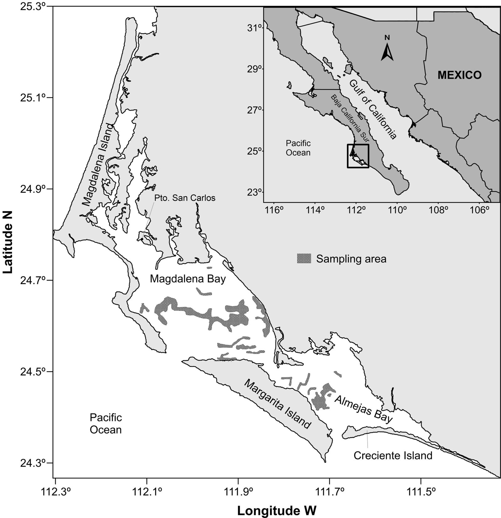
Figure 1. Location of the Bahía Magdalena-Almejas lagoon system in the northeastern Pacific of Mexico. Sampling trawl fishing sites are indicated in grey.
Based on the Red List criteria of the IUCN (IUCN, 2022), 3 (0.7%) species are “Critically Endangered” (2 chondrichthyans: the Scalloped hammerhead, Sphyraena lewini (Grifit and Smith, 1834]) and the Great hammerhead, Sphyrna mokarran (Rüpell, 1832), and the Giant seabass Stereolepis gigas Ayres, 1859); 19 (4.6%) are “Vulnerable” (6 selachians, 6 batoids and 7 actinopterygians); 6 (1.5%) are “Endangered” (4 selachians and 2 actinopterygians); 10 (2.4%) are “Near Threatened” (3 selachians and 7 batoids); 17 (4.1%) are “Not Evaluated” (all actinopterygians); 21 (5.1%) are “Data Deficient”(1 selachian, 2 batoids and 18 actinopterygians); and 340 (81%) are of “Least Concern” (6 selachians, 6 batoids and 328 actinopterygians) (Table 1). According to the latest update of the NOM-059-SEMARNAT-2010 (DOF, 2019), 2 (0.5%) species are under “Special Protection (Pr)”: the Clarion angelfish Holacanthus clarionensis Gilbert, 1891 and the Pacific seashore Hippocampus ingens Girard, 1855.
| Table 1 Systematic list of estuarine-marine fishes of the Bahía Magdalena-Almejas lagoon system (México). | ||||||
| Taxa | ZA | IUCN | NOM | D | S | H |
| Class Chondrichthyes | ||||||
| Subclass Elasmobranchii | ||||||
| Order Heterodontiformes | ||||||
| Family Heterodontidae | ||||||
| Heterodontus francisci (Girard, 1855) | SD, C, M, P | DD | ES | S | B | |
| Heterodontus mexicanus Taylor & Castro-Aguirre, 1972 | SD, C, M, P | LC | ES | S | B | |
| Order Lamniformes | ||||||
| Family Lamnidae | ||||||
| Isurus oxyrinchus Rafinesque, 1810 | CT | EN | MA | MP | ||
| Order Carcharhiniformes | ||||||
| Family Triakidae | ||||||
| Mustelus albipinnis Castro-Aguirre, Antuna-Mendiola, González-Acosta & De la Cruz-Agüero, 2005 | SD, C | LC | ES | S | D | |
| Mustelus californicus Gill, 1864 | SD, C | LC | ES | S | D | |
| Mustelus henlei (Gill, 1863) | O, SD, C, M, P | LC | ES | S | D | |
| Mustelus lunulatus Jordan & Gilbert, 1882 | SD, C, M, P | LC | ES | S | D | |
| Triakis semifasciata Girard, 1855 | O, SD, C | LC | ES | S | D | |
| Family Carcharhinidae | ||||||
| Carcharhinus albimarginatus (Rüpell, 1837) | CT | VU | MA | BP | ||
| Carcharhinus leucas (Müller & Henle, 1839) | CT | VU | ES | S | D | |
| Carcharhinus limbatus (Müller & Henle, 1839) | CT | VU | ES | S | EP | |
| Carcharhinus obscurus (Lesueur, 1818) | CT | EN | MA | MP | ||
| Galeocerdo cuvier (Péron & Lesueur, 1822) | CT | NT | MA | EP | ||
| Nasolamia velox (Gilbert, 1898) | SD, C, M, P | EN | MA | D | ||
| Negaprion brevirostris (Poey, 1868) | AA | VU | ES | R | D | |
| Prionace glauca (Linnaeus, 1758) | SD, C, M, P | NT | MA | EP | ||
| Rhizoprionodon longurio (Jordan & Gilbert, 1882) | SD, C, M, P | VU | MA | S | D | |
| Family Sphyrnidae | ||||||
| Sphyrna lewini (Griffith & Smith, 1834) | CT | CR | MA | EP | ||
| Sphyrna mokarran (Rüpell, 1837) | CT | CR | MA | EP | ||
| Sphyrna tiburo (Linnaeus, 1758) | AA | EN | ES | R | D | |
| Sphyrna zygaena (Linnaeus, 1758) | CT | VU | MA | D | ||
| Order Squaliformes | ||||||
| Family Squalidae | ||||||
| Squalus suckleyi (Girard, 1854) | AP | LC | MA | EP | ||
| Order Squatiniformes | ||||||
| Family Squatinidae | ||||||
| Squatina californica Ayres, 1859 | O, SD, C | NT | ES | S | D | |
| Subclass Batomorphii |
| Table 1 Continued. | ||||||
| Taxa | ZA | IUCN | NOM | D | S | H |
| Order Torpediniformes | ||||||
| Family Torpedinidae | ||||||
| Torpedo californica Ayres, 1855 | O, SD, C | LC | MA | R | D | |
| Family Narcinidae | ||||||
| Diplobatis ommata (Jordan & Gilbert, 1890) | SD, C, M, P | LC | ES | S | D | |
| Narcine entemedor Jordan & Starks, 1895 | SD, C, M, P | VU | ES | S | D | |
| Order Rhinopristtiformes | ||||||
| Family Rhinobatidae | ||||||
| Pseudobatos glaucostigmus (Jordan & Gilbert, 1883) | SD, C, M, P | VU | ES | S | B | |
| Pseudobatos leucorhynchus Günther, 1867 | SD, C, M, P, G | VU | ES | S | B | |
| Pseudobatos productus (Ayres, 1854) | O, SD, C | NT | ES | S | B | |
| Family Trygonorhinidae | ||||||
| Zapteryx exasperata (Jordan & Gilbert, 1880) | SD, C, M, P | DD | ES | S | D | |
| Order Myliobatiformes | ||||||
| Family Platyrhynidae | ||||||
| Platyrhinoidis triseriata (Jodan & Gilbert, 1880) | SD, C | LC | ES | S | D | |
| Family Urotrygonidae | ||||||
| Urobatis halleri (Cooper, 1863) | SD, C, M, P | LC | ES | S | B | |
| Urobatis maculatus Garman, 1913 | C, M | LC | ES | S | B | |
| Urotrygon aspidura (Jordan & Gilbert, 1882) | SD, M, P | NT | ES | S | B | |
| Urotrygon asterias (Jordan & Gilbert, 1883) | SD, C, M, P | DD | ES | S | B | |
| Urotrygon chilensis (Günther, 1872) | SD, C, M, P | NT | ES | S | B | |
| Urotrygon munda Gill, 1863 | SD, C, M, P | NT | ES | S | B | |
| Urotrygon rogersi (Jordan & Starks, 1895) | SD, C, M, P | NT | ES | S | B | |
| Family Dasyatidae | ||||||
| Hypanus dipterurus (Jordan & Gilbert, 1880) | SD, C, M, P, G | VU | MA | R | D | |
| Hypanus longus (Garman, 1880) | SD, C, M, P, G | VU | MA | R | D | |
| Family Gymnuridae | ||||||
| Gymnura marmorata (Cooper, 1864) | SD, C, M, P | NT | ES | S | D | |
| Family Aetobatidae | ||||||
| Aetobatus laticeps Gill, 1865 | SD, C, M, P | VU | ES | S | D | |
| Family Myliobatidae | ||||||
| Myliobatis californica Gill, 1865 | O, SD, C, M, P | LC | MA | EP | ||
| Myliobatis longirostris Applegate & Fitch, 1964 | SD, C, M, P | VU | ES | S | D | |
| Family Rhinopteridae | ||||||
| Rhinoptera steindachneri Evermann & Jenkins, 1891 | SD, C, M, P, G | NT | MA | S | EP | |
| Class Actinopterygii | ||||||
| Order Elopiformes | ||||||
| Family Elopidae | ||||||
| Elops affinis Regan, 1909 | SD, C, M, P | DD | ES | S | EP | |
| Order Albuliformes | ||||||
| Family Albulidae | ||||||
| Albula gilberti Pfeiler & van der Heiden, 2011 | SD, C | NE | ES | S | D | |
| Order Angulliformes | ||||||
| Family Muraenidae | ||||||
| Echidna nocturna (Cope, 1872) | CT | LC | ES | R | D | |
| Gymnothorax castaneus (Jordan & Gilbert, 1883) | SD, C, M, P, G | LC | ES | R | D | |
| Gymnothorax mordax (Ayres, 1859) | SD, C, M, P, G | LC | MA | R | D | |
| Gymnothorax verrilli (Jordan & Gilbert, 1883) * | SD, C, M, P | LC | ES | S | D | |
| Muraena argus (Steindachner, 1870) | SD, C, M, P, G | LC | MA | R | D | |
| Muraena lentiginosa Jenyns, 1842 * | SD, C, M, P | LC | MA | R | D | |
| Family Ophichthidae | ||||||
| Myrichthys tigrinus Girard, 1859 | SD, C, M, P, G | LC | ES | S | D | |
| Myrophis vafer Jordan & Gilbert, 1883 | SD, C, M, P, G | LC | ES | S | D | |
| Ophichthus triserialis (Kaup, 1856) | O, SD, C, M, P, G | LC | ES | S | D | |
| Ophichthus zophochir Jordan & Gilbert, 1882 | O, SD, C, M, P, G | LC | ES | S | D | |
| Family Congridae | ||||||
| Ariosoma gilberti (Ogilby, 1898) | C, M, P, G | LC | ES | S | B | |
| Gorgasia puntata Meek & Hildebrand, 1923 | SD, C, M, P | LC | ES | S | D | |
| Order Clupeiformes | ||||||
| Family Engraulidae | ||||||
| Anchoa argentivittata (Regan, 1904) | SD, C, M, P | LC | ES | EP | ||
| Anchoa compressa (Girard, 1858) | SD, C | LC | ES | EP | ||
| Anchoa delicatissima (Girard, 1854) | O, SD | LC | ES | EP | ||
| Anchoa exigua (Jordan & Gilbert, 1882) | SD, C, M | LC | ES | EP | ||
| Anchoa helleri (Hubbs, 1921) | SD, C | LC | ES | EP | ||
| Anchoa ischana (Jordan & Gilbert, 1882) | SD, C, M, P | LC | ES | EP | ||
| Anchoa lucida (Jordan & Gilbert, 1882) | SD, C, M | LC | ES | EP | ||
| Anchoa nasus (Kner & Steichnader, 1867) | SD, C, M, P | LC | ES | EP | ||
| Anchovia macrolepidota (Kner, 1863) | SD, C, M, P | LC | ES | EP | ||
| Cetengraulis mysticetus (Günther, 1867) * | SD, C, M, P | LC | ES | EP | ||
| Engraulis mordax Girard, 1854 | SD, C, M, P | DD | ES | EP | ||
| Family Clupeidae | ||||||
| Harengula thrissina (Jordan & Gilbert, 1882) * | S, C, M, P, G | LC | ES | EP | ||
| Lile nigrofasciata Castro-Aguirre, Ruiz-Campos & Balart, 2002 | SD, C, M, P | LC | ES | EP | ||
| Lile stolifera (Jordan & Gilbert, 1882) | SD, C, M, P | LC | ES | EP | ||
| Opisthonema libertate (Günther, 1867) | SD, C, M, P | LC | ES | EP | ||
| Opisthonema medirastre Berry & Barret, 1963 * | SD, C, M, P | LC | ES | EP | ||
| Sardinops sagax (Jenyns, 1842) * | CT | LC | ES | EP | ||
| Family Drussumieriidae | ||||||
| Etrumeus acuminatus Gilbert, 1890 * | SD, C, M, P | LC | MA | EP | ||
| Order Gonorynchiformes | ||||||
| Family Chanidae | ||||||
| Chanos chanos (Forsskål, 1775) | CT | LC | ME | EP | ||
| Order Siluriformes | ||||||
| Family Ariidae | ||||||
| Bagre panamensis (Gill, 1863) | SD, C, M, P | LC | ME | S | EP | |
| Notarius planiceps (Steindachner, 1876) | SD, C, M, P | LC | ME | S | EP | |
| Occidentarius platypogon (Günther, 1864) | SD, C, M, P | LC | ME | S | EP | |
| Order Stomiiformes | ||||||
| Family Phosichthydae | ||||||
| Vicinguerria lucetia (Garman, 1899) * | AP | LC | MA | EP | ||
| Order Aulopiformes | ||||||
| Family Synodontidae | ||||||
| Synodus evermanni Jordan & Bollman, 1890 | SD, C, M, P | LC | ES | S | D | |
| Synodus lacertinus Gilbert, 1890 | SD, C, M, P, G, PC | LC | ES | R | D | |
| Synodus lucioceps (Ayres, 1855) | SD, C, M | LC | ES | S | D | |
| Synodus scituliceps Jordan & Gilbert, 1882 | SD, C, M, P | LC | ES | S | D | |
| Synodus sechurae Hildebrand, 1946 | SD, C, M, P | LC | ES | S | D | |
| Order Myctophiformes | ||||||
| Family Myctophidae | ||||||
| Ceratoscopelus townsendi (Eigenmann & Eigenmann, 1889) * | CT | LC | MA | EP | ||
| Ceratoscopelus warmingii (Lütken, 1892) | CT | LC | MA | EP | ||
| Electrona risso (Cocco, 1829) | CT | LC | MA | EP | ||
| Lampadena urophaos Paxton, 1963 | CT | LC | MA | EP | ||
| Order Gadiformes | ||||||
| Family Merluccidae | ||||||
| Merluccius productus (Ayres, 1853) | SD, C, M | LC | MA | D | ||
| Order Ophidiiformes | ||||||
| Family Ophidiidae | ||||||
| Chilara taylori (Girard, 1858) | SD, C, M, P | LC | ES | S | D | |
| Lepophidium negropinna (Hildebrand & Barton, 1949) * | SD, C, M, P, PC | LC | ES | S | D | |
| Ophidion galeoides (Gilbert, 1890) | SD, C, M, P | LC | ES | S | D | |
| Ophidion scrippsae (Hubbs, 1916) ¨* | SD, C | LC | ES | S | D | |
| Family Dinematichthyidae | ||||||
| Ogilbia ventralis (Gill, 1863) | SD, C, M, P, G | LC | MA | S | D | |
| Order Batrachoidiformes | ||||||
| Family Batrachoididae | ||||||
| Porichthys analis Hubbs & Schultz, 1939 | SD, C, M, P | LC | ES | D | ||
| Porichthys margaritatus (Richardson, 1844) | SD, C, M | LC | ES | D | ||
| Porichthys myriaster Hubbs & Schultz, 1939 | SD, C, M, P | LC | ES | S | D | |
| Porichthys notatus Girard, 1854 | O, SD, C | LC | ES | S | D | |
| Order Lophiiformes | ||||||
| Family Lophiidae | ||||||
| Lophioides caulinaris (Garman, 1899) | SD, C, M, P, G | LC | MA | D | ||
| Lophioides setigerus (Vahl, 1797) | CT | LC | MA | D | ||
| Lophioides spilurus (Garman, 1899) | SD, C, M, P | LC | MA | B | ||
| Family Antennariidae | ||||||
| Fowlerichthys avalonis (Jordan & Starks, 1907) | SD, C, M, P, G | LC | ES | S | D | |
| Family Ogcocephalidae | ||||||
| Zalieutes elater (Jordan & Gilbert, 1882) | SD, C, M, P, G | LC | ES | S | D | |
| Order Mugiliformes | ||||||
| Family Mugilidae | ||||||
| Chaenomugil proboscideus (Günther, 1861) | SD, C, M, P | LC | ES | R | EP | |
| Mugil cephalus Linnaeus, 1758 | CT | LC | ES | S | D | |
| Mugil curema Valenciennes, 1836 | CT | LC | ES | S | D | |
| Mugil hospes Jordan & Culver, 1895 | AA | LC | ES | S | D | |
| Mugil setosus Gilbert, 1892 | SD, C, M, P | LC | MA | D | ||
| Order Atheriniformes | ||||||
| Family Atherinopsidae | ||||||
| Atherinella eriarcha Jordan & Gilbert, 1882* | SD, C, M | LC | ES | EP | ||
| Atherinella nepenthe (Myers & Wade, 1942) * | SD, C, M, P | LC | ES | EP | ||
| Atherinops affinis (Ayres, 1860) * | O, SD, C | LC | ES | EP | ||
| Atherinopsis californiensis Girard, 1854 * | O, SD, C | LC | ES | EP | ||
| Leuresthes tenuis (Ayres, 1860) | O, SD, C | NE | MA | EP | ||
| Order Beloniformes | ||||||
| Family Exocoetidae | ||||||
| Fodiator acutus (Valenciennes, 1847) * | SD, C, M, P | LC | MA | EP | ||
| Prognichthys tringa Breder, 1928 * | SD, C, M, P, G | LC | MA | EP | ||
| Family Hemirhamphidae | ||||||
| Hemirhamphus saltator Gilbert & Starks, 1904 * | O, SD, C, M, P | LC | ES | EP | ||
| Hyporhamphus gilli Meek & Hildebrand, 1923 | SD, C, M, P, G | LC | ES | EP | ||
| Hyporhamphus naos Banford & Collette, 2001 | SD, C, M, P | LC | ES | EP | ||
| Hyporhamphus rosae (Jordan & Gilbert, 1880) * | SD, C, M, P | LC | ES | EP | ||
| Oxyporhamphus micropterus (Valenciennes, 1847) * | CT | NE | MA | EP | ||
| Family Belonidae | ||||||
| Strongylura exilis (Girard, 1854) * | SD, C, M, P | LC | ES | EP | ||
| Order Cyprinodontiformes | ||||||
| Family Fundulidae | ||||||
| Fundulus parvipinnis Girard, 1854 | O, SD | LC | ES | S | D | |
| Order Gasterosteiformes | ||||||
| Family Syngnathidae | ||||||
| Cosmocampus arctus (Jenkins & Evermann, 1889) * | SD, C | LC | ES | R | D | |
| Doryrhamphus excisus Kaup, 1856 | CT | LC | ES | R | D | |
| Hippocampus ingens Girard, 1858 * | SD, C, M, P | VU | Pr | ES | S | D |
| Syngnathus auliscus (Swain, 1882) * | SD, C, M, P | LC | ES | S | D | |
| Syngnathus exillis (Osburn & Nichols, 1916) | O, SD | LC | ES | S | D | |
| Syngnathus leptorhynchus Girard, 1854 * | O, SD | LC | ES | S | D | |
| Family Fistularidae | ||||||
| Fistularia commersonii Rüpell, 1838 | AP | LC | ES | S | D | |
| Fistularia corneta Gilbert & Starks, 1904 | SD, C, M, P, G | LC | ES | S | D | |
| Order Scorpaeniformes | ||||||
| Family Scorpaenidae | ||||||
| Scorpaena guttata Girard, 1854 | SD, C | DD | MA | R | D | |
| Scorpaena mystes Jordan & Starks, 1895 | SD, C, M, P, G | LC | MA | R | D | |
| Scorpaena russula Jordan & Bollman, 1890 | SD, C, M, P | LL | MA | R | B | |
| Scorpaena sonorae Jenkins & Evermann, 1889 | SD, C | LC | MA | R | B | |
| Sebastes auriculatus Girard, 1854 | O, SD | NE | MA | R | B | |
| Sebastes goodei (Eigenmann & Eigenmann, 1890) | O, SD | NE | MA | R | D | |
| Family Triglidae | ||||||
| Bellator gymnostethus (Gilbert, 1892) | SD, C, M, P | LC | MA | B | ||
| Bellator loxias (Jordan, 1897) | SD, C, M, P, G | LC | MA | B | ||
| Bellator xenisma (Jordan & Bollman, 1890) | O, SD, C, M, P | LC | MA | B | ||
| Prionotus birostratus Richardson, 1844 | SD, C, M, P | LC | MA | B | ||
| Prionotus horrens Richardson, 1844 | SD, C, M, P | LC | MA | B | ||
| Prionotus ruscarius Gilbert & Starks, 1904 * | SD, C, M, P | LC | MA | B | ||
| Prionotus stephanophrys Lockington, 1881 | SD, C, M, P | LC | MA | B | ||
| Family Scorpaenichthyidae | ||||||
| Scorpaenichthys marmoratus (Ayres, 1854) * | O, SD | NE | MA | B | ||
| Family Psychrolutidae | ||||||
| Chitonotus pugetensis (Steindachner, 1876) | O, SD | NE | MA | B | ||
| Family Agonidae | ||||||
| Stellerina xyosterna (Jordan & Gilbert, 1880) | O,SD | NE | MA | B | ||
| Order Perciformes | ||||||
| Family Centropomidae | ||||||
| Centropomus medius Günther, 1864 | SD, C, M, P | LC | ES | S | B | |
| Centropomus nigrescens Günther, 1864 | SD, C, M, P | LC | ES | S | B | |
| Family Polyprionidae | ||||||
| Stereolepis gigas Ayres, 1859 | SD, C | CR | ES | S | D | |
| Family Epinephelidae | ||||||
| Cephalopholis panamensis (Steindachner, 1877) | SD, C, M, P | LC | MA | R | D | |
| Dermatolepis dermatolepis (Boulenger, 1895) | SD, C, M, P, G | LC | ES | R | D | |
| Epinephelus analogus Gill, 1863 | SD, C, M, P, G | LC | ES | S | D | |
| Epinephelus labriformis (Jenyns, 1840) | SD, C, M, P, G | LC | MA | R | D | |
| Epinephelus quinquefasciatus (Bocourt,1868) | SD, C, M, P | DD | ES | S | D | |
| Hyportodus niphobles (Gilbert & Starks, 1897) | SD, C, M, P | LC | ES | D | ||
| Mycteroperca jordani (Jenkins & Evermann, 1889) | SD, C, M | EN | ES | D | ||
| Mycteroperca rosacea (Streets, 1877) | SD, C, M | LC | ES | D | ||
| Mycteroperca xenarcha Jordan, 1888 | SD, C, M, P | DD | MA | R | D | |
| Rypticus bicolor Valenciennes, 1846 | SD, C, M, P, G | LC | ES | R | D | |
| Rypticus nigripinnis Gill, 1861 | SD, C, M, P, G | LC | ES | S | D | |
| Family Serranidae | ||||||
| Diplectrum eumelum Rosenblatt & Johnson, 1974 | SD, C, M, P, G | LC | MA | S | D | |
| Diplectrum euryplectrum Jordan & Bollman, 1890 | SD, C, M, P | LC | MA | S | D | |
| Diplectrum labarum Rosenblatt & Johnson, 1974 | SD, C, M, P | LC | MA | S | MP | |
| Diplectrum macropoma (Gpunther, 1864) | SD, C, M, P, G | LC | MA | S | D | |
| Diplectrum maximum Hildebrand, 1946 | O, SD, C, M, P | LC | MA | S | B | |
| Diplectrum pacificum Hildebrand, 1946 | SD, C, M, P | LC | ES | S | D | |
| Diplectrum rostrum Bortone, 1974 | SD, C, M, P, G | LC | MA | S | D | |
| Diplectrum sciurus Gilbert, 1892 | SD, C | LC | MA | S | D | |
| Paralabrax aeroguttatus Waldford, 1936 * | SD, C | DD | MA | R | D | |
| Paralabrax clathratus (Girard, 1854) | O, SD | LC | MA | R | D | |
| Paralabrax maculatofasciatus (Steindachner, 1868) * | SD, C, M, P | LC | MA | S | D | |
| Paralabrax nebulifer (Girard, 1854) * | SD, C, M | LC | MA | R | D | |
| Family Opistognhtidae | ||||||
| Opistognathus punctatus Peters, 1869 | SD, C, M, P, G | LC | MA | S | D | |
| Opistognathus rhomaleus Jordan & Gilbert, 1881 | SD, C, M, P | LC | MA | S | D | |
| Family Priacanthidae | ||||||
| Cookeolus japonicus (Cuvier, 1829) | CT | LC | MA | R | D | |
| Pristigenys serrula (Gilbert, 1891) | SD, C,M, P | LC | MA | R | D | |
| Family Apogonidae | ||||||
| Apogon atricaudus Jordan & McGregor, 1898* | SD, C, M | LC | MA | R | D | |
| Apogon guadalupensis (Osburn & Nichols, 1916) | SD, C, M, G | LC | MA | R | D | |
| Apogon pacificus (Herre, 1935) | SD, C, M, P, G | LC | MA | R | D | |
| Apogon retrosella (Gill, 1862)* | SD, C, M | LC | MA | R | D | |
| Family Malacanthidae | ||||||
| Caulolatilus affinis Gill, 1865 | SD, C, M, P, G | LC | MA | S | D | |
| Caulolatilus princeps (Jenyns, 1840) | O, SD, C, M, P, G | LC | MA | S | D | |
| Family Nematistiidae | ||||||
| Nematistius pectoralis Gill, 1862 | SD, C, M, P | NE | ES | S | D | |
| Family Carangidae | ||||||
| Alectis ciliaris (Bloch, 1787) | CT | LC | ES | S | D | |
| Carangoides otrynter Jordan & Gilbert, 1883 | SD, C, M, P, G | LC | ES | S | D | |
| Carangoides vinctus Jordan & Gilbert, 1882 | SD, C, M, P | LC | MA | S | EP | |
| Caranx caballus Günther, 1868 | SD, C, M, P | LC | ES | S | EP | |
| Chloroscombrus orqueta Jordan & Gilbert, 1883 * | SD, C, M, P | LC | ES | S | D | |
| Decapterus macrosoma Bleeker, 1851 | CT | LC | MA | EP | ||
| Gnathanodon speciosus (Forsskål, 1775) * | CT | LC | ES | S | D | |
| Hemicaranx leucurus (Günther, 1864) | SD, C, M, P | LC | ES | S | D | |
| Hemicaranx zelotes Gilbert, 1898 | O, SD, C, M, P | LC | ES | S | D | |
| Oligoplites altus (Günther, 1868) | SD, C, M, P, PC | LC | ES | S | D | |
| Oligoplites saurus (Bloch & Schneider, 1801) * | SD, C, M, P | LC | ES | S | D | |
| Selene brevoortii (Gill, 1863) | SD, C, M, P | LC | ES | S | D | |
| Selene orstedii Lütken, 1880 | SD, C, M, P, G | LC | ES | S | D | |
| Selene peruviana (Guichenot, 1866) * | SD, C, M, P | LC | ES | S | D, MP | |
| Seriola lalandi Valenciennes, 1833 | CT | LC | ES | S | D, MP | |
| Trachinotus kennedyi Steindachner, 1876 | SD, C, M, P | LC | ES | S | D, MP | |
| Trachinotus paitensis Cuvier, 1832 | SD, C, M, P | LC | ES | S | D, MP | |
| Trachurus symmetricus (Ayres, 1855) | SD, C, M, P | LC | MA | D, MP | ||
| Family Coryphaenidae | ||||||
| Coryphaena hippurus Linnaeus, 1758 | CT | LC | MA | EP | ||
| Family Lutjanidae | ||||||
| Hoplopagrus guentherii Gill, 1862 | SD, C, M, P | LC | ES | S, R | D | |
| Lutjanus aratus (Günther, 1864) | SD, C, M, P | LC | ES | S, R | D | |
| Lutjanus argentiventris (Peters, 1869) * | SD, C, M, P | LC | ES | S, R | D | |
| Lutjanus colorado Jordan & Gilbert, 1882 | SD, C, M, P | LC | ES | S, R | D | |
| Lutjanus guttatus (Steindachner, 1869) | SD, C, M, P | LC | ES | S, R | D | |
| Lutjanus inermis (Peters, 1869) | SD, C, M, P | LC | MA | R | D | |
| Lutjanus jordani (Gilbert, 1898) | SD, C, M, P, G | LC | ES | S, R | D | |
| Lutjanus novemfasciatus Gill, 1862 | SD, C, M, P | LC | ES | S | D | |
| Lutjanus peru (Nichols & Murphy, 1922) | SD, C, M, P, G | LC | MA | S, R | D | |
| Family Lobotidae | ||||||
| Lobotes pacificus Gilbert, 1898 | SD, C, M, P | LC | ES | S | D | |
| Family Gerreidae | ||||||
| Dekertichthys aureolus (Jordan & Gilbert, 1882) | SD, C, M, P | NE | ES | S | D | |
| Diapterus brevirostris (Sauvage, 1879) * | SD, C, M, P | NE | ES | S | D | |
| Eucinostomus currani Zahuranec, 1980 * | SD, C, M, P | LC | ES | S | D | |
| Eucinostomus dowii (Gill, 1863) * | SD, C, M, P | LC | ES | S | D | |
| Eucinostomus entomelas Zahuranec, 1980 | SD, C, M, P | LC | ES | S | D | |
| Eucinostomus gracilis (Gill, 1862) * | SD, C, M, P | LC | ES | S | D | |
| Eugerres lineatus (Humboldt, 1821) | SD, C, M, P | LC | ES | S | D | |
| Gerres cinereus (Walbaum, 1792) | AA | LC | ES | S | D | |
| Family Haemulidae | ||||||
| Anisotremus davidsonii (Steindachner, 1875) | SD, C | LC | MA | R | D | |
| Anisotremus interruptus (Gill, 1862) | SD, C, M, P, G | LC | MA | R | D | |
| Brachygenys californiensis (Steindachner, 1875) | SD, C | LC | MA | R | D | |
| Conodon serrifer Jordan & Gilbert, 1882 | SD, C, M, P | LC | ES | S | D | |
| Haemulon flaviguttatum Gill, 1862 | SD, C, M, P | LC | MA | R | D | |
| Haemulon maculicauda (Gill, 1862) | SD, C, M, P, G | LC | MA | R | D | |
| Haemulon scudderi Gill, 1862 | SD, C, M, P, G | LC | ES | S, R | D | |
| Haemulon sexfasciatum Gill, 1862 | SD, C, M, P | LC | MA | S, R | D | |
| Haemulon steindachneri (Jordan & Gilbert, 1882) | AA | LC | ES | S, R | D | |
| Haemulopsis axillaris (Steindachner, 1869) | SD, C, M, P | LC | ES | S | D | |
| Haemulopsis elongatus (Steindachner, 1879) | SD, C, M, P | LC | ES | S | D | |
| Haemulopsis leuciscus (Günther, 1864) | SD, C, M, P | LC | ES | S | D | |
| Hamulopsis nitidus (Steindachner, 1869) | SD, C, M, P | LC | ES | S | D | |
| Microlepidotus inornatus Gill, 1862 | SD, C, M | LC | ES | S | D | |
| Orthopristis cantharinus (Jenyns, 1840) | SD, C, M, P, G | DD | ES | S | D | |
| Orthopristis chalceus (Günther, 1864) | SD, C, M, P, G | LC | ES | S | D | |
| Orthopristis reddingi Jordan & Richardson, 1895 | SD, C, M, P | LC | ES | S | D | |
| Rhencus macracanthus (Günther, 1864) | SD, C, M, P | LC | ES | S | D | |
| Rhencus panamensis (Steindachner, 1875) | SD, C, M, P | LC | ES | S | D | |
| Rhonciscus bayanus (Jordan & Evermann, 1898) | SD, C, M, P | LC | ES | S | D | |
| Pomadasys branickii (Steindachner, 1879) | SD, C, M, P | LC | ES | S | D | |
| Xenichthys xanti Gill, 1863 | SD, C, M, P | LC | MA | R | D | |
| Family Sparidae Gill 1863 | ||||||
| Calamus brachysomus (Lokington, 1880) * | SD, C, M, P | LC | ES | S | D | |
| Family Polynemidae | ||||||
| Polydactylus approximans (Lay & Bennett, 1839) * | O, SD, C, M, P | LC | ES | S | D | |
| Poldactylus oprecularis (Gill, 1863) | SD, C, M, P, PC | LC | ES | S | D | |
| Family Sciaenidae | ||||||
| Atractoscion nobilis (Ayres, 1860) | O, SD, C | LC | ES | S | D | |
| Bairdiella armata Gill, 1863 | SD, C | LC | ES | S | D | |
| Bairdiella icistia (Jordan & Gilbert, 1882) * | C, M, P, G | LC | ES | S | D | |
| Cheilotrema saturnum (Girard, 1858) | O, SD, C, M, P | DD | MA | R | D | |
| Corvula macrops (Steindachner, 1985) | SD, C, M, P, G | DD | MA | R | D | |
| Cynoscion parvipinnis Ayres, 1861 | O, SD, C | DD | ES | S | D | |
| Cynoscion reticulatus (Günther, 1864) | SD, C, M, P | LC | ES | S | D | |
| Cynoscion squamipinnis (Günther, 1867) | SD, C, M, P | LC | ES | S | D | |
| Cynoscion xanthulus Jordan & Gilbert, 1882 | SD, C, M, P | LC | ES | S | D | |
| Elattarchus archidium (Jordan & Gilbert, 1882) | SD, C, M, P | LC | ES | S | D | |
| Genyonemus lineatus (Ayres, 1855) | O, SD | LC | MA | S | D | |
| Larimus pacificus Jordan & Bollman, 1890 | SD, C, M, P, G, PC | LC | ES | S | D | |
| Menticirrhus elongatus (Günther, 1864) | SD, C, M, P | LC | ES | S | D | |
| Menticirrhus nasus (Günther, 1868) | SD, C, M, P | LC | ES | S | D | |
| Menticirrhus panamensis (Steindachner, 1875) | SD, C, M, P, PC | LC | ES | S | D, MP | |
| Menticirrhus undulatus (Girard, 1854) * | SD, C, M, P | DD | ES | S | D, MP | |
| Micropogonias altipinnis (Günther, 1864) | SD, C, M, P | LC | ES | S | D | |
| Micropogonias ectenes (Jordan & Gilbert, 1882) * | SD, C, M, P | LC | ES | S | D, MP | |
| Ophioscion vermicularis (Günther, 1867) | SD, C, M, P | LC | ES | S | D | |
| Paralonchurus goodei Gilbert, 1898 | SD, C, M, P | LC | ES | S | D | |
| Pareques viola (Gilbert, 1898) | SD, C, M, P | LC | MA | S | D | |
| Roncador stearnsii (Steindachner, 1876) | SD, C, M | LC | ES | S | D | |
| Seriphus politus Ayres, 1860 | O, SD | LC | ES | D, MP | ||
| Stellifer winterteenorum Chao, 2001 | SD, C, M | NE | ES | S | D | |
| Umbrina roncador Jordan & Gilbert, 1882 | C, M | LC | ES | S | D | |
| Umbrina winterteeni Walker & Radford, 1992 | SD, C | DD | ES | S | D | |
| Umbrina xanti Gill, 1862 | SD, C, M, P | LC | ES | S | D | |
| Family Mullidae | ||||||
| Mulloidichthys dentatus (Gill, 1862) | SD, C, M, P | LC | MA | S | D | |
| Pseudupeneus grandisquamis (Gill, 1863) | SD, C, M, P, G | LC | MA | S | D | |
| Family Kyphosidae | ||||||
| Kyphosus azureus (Jenkins & Evermann, 1889) | O, SD, C | LC | ES | R | D | |
| Kyphosus elegans (Peters, 1869) | SD, C, M, P, G | LC | ES | R | D | |
| Kyphosus vaigiensis (Qouy & Gaimard, 1825) | SD, C, M, P, G | LC | MA | R | D | |
| Family Chaetodontidae | ||||||
| Chaetodon humeralis Günther, 1860 | SD, C, M, P, G | LC | MA | R | D | |
| Prognathodes falcifer (Hubbs & Rechnitzer, 1958) | SD, C, M, G | LC | MA | R | D | |
| Family Pomacanthidae | ||||||
| Holocanthus clarionensis Gilbert, 1891 | SD, C, M, P | VU | Pr | MA | S, R | D |
| Holacanthus passer Valenncienes, 1846 | SD, C, M, P | LC | MA | S, R | D | |
| Family Cirrhitidae | ||||||
| Cirrhitus rivulatus Valenciennes, 1846 | SD, C, M, P | LC | MA | D | ||
| Oxyrrhites typus Bleeker, 1857 | CT | LC | MA | R | D | |
| Family Embiotocidae | ||||||
| Embiotoca jacksoni Agazziz, 1853 | SD, C | LC | MA | MP | ||
| Family Pomacentridae | ||||||
| Abudefduf declivifrons (Gill, 1862) | SD, C, M, P | LC | MA | S, R | D | |
| Abudefduf troschelii (Gill, 1862) * | SD, C, M, P | LC | MA | S, R | D | |
| Hypsypops rubicundus (Girard, 1854) * | SD, C, M | LC | MA | R | D | |
| Microspathodon dorsalis (Gill, 1862) | SD, C, M, P, G | LC | MA | R | D | |
| Stegastes acapulcoensis (Fowler, 1944) | SD, C, M, P, G | LC | MA | R | D | |
| Stegastes leucorus (Gilbert, 1892) | SD, C, M, P, G | VU | MA | R | D | |
| Stegastes rectifraenum (Gill, 1862) | SD, C, M | LC | MA | R | D | |
| Stegastes redemptus (Heller & Snodgrass, 1903) | SD | LC | MA | R | D | |
| Family Labridae | ||||||
| Bodianus diplotaenia (Gill, 1862) * | SD, C, M, P, G | LC | MA | R | D | |
| Bodianus pulcher (Ayres, 1854) | O, SD, C | VU | MA | R | D | |
| Halichoeres californicus (Günther, 1861) * | O, SD | LC | MA | S, R | D | |
| Halichoeres chierchiae DiCaporiacco, 1947 | SD, C, M, P | LC | MA | R | D | |
| Halichoeres notospilus (Günther, 1864) | SD, C, M, P, G | LC | ES | S, R | D | |
| Halichoeres semicinctus (Ayres, 1859) | SD, C | LC | MA | R | D | |
| Thalassoma grammaticum Gilbert, 1890 | SD, C, M, P | LC | MA | R | D | |
| Thalassoma lucasanum (Gill, 1862) | SD, C, M, P | LC | MA | S, R | D | |
| Xyrichtys mundiceps Gill, 1862 | SD, C, M | LC | ES | S | D | |
| Family Scaridae | ||||||
| Nicholsina denticulata (Evermann & Radcliffe, 1917) | SD, C, M, P, G | LC | MA | S, R | D | |
| Scarus compressus (Osburn & Nichols, 1916) | SD, C, M, P, G | LC | MA | S, R | D | |
| Scarus ghobban Forsskål, 1775 | CT | LC | MA | S, R | D | |
| Scarus perrico Jordan & Gilbert, 1882 | SD, C, M, P, G | LC | MA | S, R | D | |
| Family Uranoscopidae | ||||||
| Astroscopus zephyreus Gilbert & Starks, 1897 | SD, C, M, P | LC | MA | S | D | |
| Kathetostoma averruncus Jordan & Bollman, 1890 | O, SD, C, M, P, G | LC | MA | S | D | |
| Family Tripterygiidae | ||||||
| Axoclinus storeyae (Brock, 1940) | SD, C | LC | MA | S, R | D | |
| Enneanectes carminalis (Jordan & Gilbert, 1882) * | SD, C, M, P | LC | MA | R | D | |
| Family Dactyloscopidae | ||||||
| Dactylagnus mundus Gill, 1862 | SD, C, M, P, G | LC | MA | S | D | |
| Dactyloscopus elongatus Myers & Wade, 1946 | SD, C, M | LC | MAR | S | D | |
| Dactyloscopus pectoralis Gill, 1861 | SD, C, M | NE | MA | S | D | |
| Gillellus semicinctus Gilbert, 1890 | SD, C, M, P, G | LC | MAR | S | D | |
| Heteristius cinctus (Osburn & Nichols, 1916) | SD, C, M, P | LC | MAR | S | D | |
| Family Blennidae | ||||||
| Hypsoblennius brevipinnis (Günther, 1861) | SD, C, M, P, G | LC | MAR | R | B | |
| Hypsoblennius gentilis (Girard, 1840) * | SD, C | LC | ES | R | B | |
| Hypsoblennius gilberti (Jordan, 1882) * | O, SD | LC | MAR | R | D | |
| Hypsoblennius jenkinsi (Jordan & Evermann, 1896) * | SD, C | LC | MA | R | D | |
| Ophioblennius steindachneri Jordan & Evermann, 1898 * | SD, C, M, P, G | LC | MAR | R | D | |
| Plagiotremus azaleus (Jordan & Bollman, 1890) | SD, C, M, P, G | LC | MAR | R | D | |
| Family Clinidae | ||||||
| Gibbonsia elegans (Cooper, 1864) | O, SD, C | LC | MA | S | B | |
| Family Labrisomidae | ||||||
| Labrisomus multiporosus Hubb, 1953 * | SD, C, M, P, G | LC | MA | R | B | |
| Labrisomus xanti Gill, 1860* | SD, C, M, G | LC | MA | R | B | |
| Malacoctenus hubbsi Springer, 1959 * | SD, C | LC | MA | R | B | |
| Malacoctenus tetranemus (Cope, 1877) | SD, C, M, P, G | LC | MA | R | B | |
| Paraclinus asper (Jenkins & Evermann, 1889) * | SD, C | LC | MA | R | B | |
| Paraclinus integripinnis (Smith, 1880) * | SD, C, M | LC | MA | R | B | |
| Paraclinus magdalenae Rosenblatt & Parr, 1969 | SD, E | EN | MA | R | B | |
| Paraclinus sini Hubbs, 1952 | SD, C | LC | MA | R | B | |
| Paraclinus stephensi Rosenblatt & Parr, 1969 | SD, M | LC | MA | R | B | |
| Family Chaenopsidae | ||||||
| Chaenopsis alepidota (Gilbert, 1890) * | SD, C, M, P | LC | MA | S | B | |
| Cirriemblemaria lucasana (Stephens, 1963) | SD, C, M | LC | MA | R | B | |
| Coralliozetus micropes (Beebe & Tee-Van, 1938) | SD, C | LC | MA | R | B | |
| Coralliozetus rosenblatti Stephens, 1963 | SD, C | LC | MA | R | B | |
| Protemblemaris bicirrus (Hildebrand, 1946) | SD, C, M, P | LC | MA | R | B | |
| Stathmonotus sinuscalifornici (Chabanaud, 1842) * | SD, C | LC | MA | R | B | |
| Family Gobioesocidae | ||||||
| Gobiesox papillifer Gilbert, 1890 | SD, C, M, P | LC | MA | R | B | |
| Rimicola eigenmanni (Gilbert, 1890) | SD | NE | MA | R | B | |
| Tomicodon zebra (Jordan & Gilbert, 1882) | SD, C, M, P | LC | MA | R | B | |
| Family Callionymidae | ||||||
| Synchiropus atrilabiatus (Garmann, 1899) | SD, C, M, P, G | LC | MA | S | D | |
| Family Eleotridae | ||||||
| Gobiomorus maculatus (Günther, 1859) | SD, C, M, P, G | LC | ES | S | D | |
| Family Gobiidae | ||||||
| Bathygobius ramosus Ginsburg, 1947 | SD, C, M, P | LC | ES | S | B | |
| Ctenogobius sagittula (Günther, 1861) | SD, C, M, P | LC | ES | S | B | |
| Coryphopterus urospilus Ginsburg, 1938 | SD, C, M, P, G | LC | MA | R | B | |
| Gillichthys mirabilis (Cooper, 1864) * | O, SD, C | LC | ES | S | B | |
| Gobulus crescentalis (Gilbert, 1892) | SD, C, M, P | LC | MA | R | B | |
| Gymneleotris seminuda (Günther, 1864) | SD, C, M, P | LC | MA | R | B | |
| Ilypnus gilberti (Eigenmann & Eigenmann, 1889) * | O, SD | LC | ES | S | B | |
| Lythrypnus dalli (Gilbert, 1890) * | SD, C, M, P, G | LC | MA | R | B | |
| Lythrypnus pulchellus Ginsburg, 1938 | SD, C, M, P | LC | MA | R | B | |
| Lythrypnus zebra (Gilbert, 1890) * | O, SD, C | LC | MA | R | B | |
| Microgobius erectus Ginsburg, 1938 | SD, C, M, P | LC | ES | S | B | |
| Microgobius miraflorensis Gilbert & Starks, 1904 | SD, C, M, P | LC | ES | S | B | |
| Microgobius tabogensis Meek & Hildebrand, 1928 | SD, C, M, P | LC | ES | S | B | |
| Quietula y-cauda (Jenkins & Evermann, 1889) * | SD, C | LC | ES | S | B | |
| Typlogobius californiensis Steindachner, 1879 | SD | NE | MA | R | B | |
| Family Microdesmidae | ||||||
| Microdesmus dorsipunctatus Dawson, 1968 | SD, C, M, P | DD | ES | S | B | |
| Family Ephippidae | ||||||
| Chaetodipterus zonatus (Girard, 1858) * | SD, C, M, P | LC | ES | S | D | |
| Family Zanclidae | ||||||
| Zanclus cornutus (Linnaeus, 1758) | CT | NE | MA | R | D | |
| Famila Acanthuridae | ||||||
| Prionotus laticlavius (Valenncienes, 1846) | SD, C, M, P | LC | MA | R | D | |
| Family Sphyraenidae | ||||||
| Sphyraena argentea Girard, 1854 | O, SD, C | LC | MA | S | D | |
| Sphyraena ensis Jordan & Gilbert, 1882 * | SD, C, M, P. PC | LC | MA | S | D | |
| Sphyraena lucasana Gill, 1863 | SD, C, M, P | DD | MA | S | D | |
| Family Scombridae | ||||||
| Auxis thazard (Lacepède, 1800) | CT | LC | MA | D | ||
| Euthynnus affinis (Cantor, 1849) | CT | LC | MA | D | ||
| Sarda chiliensis (Cuvier, 1832) | O, SD, C, M, P, PC | LC | MA | D | ||
| Scomber japonicus Houttuyn, 1782 | CT | LC | MA | D | ||
| Scomberomorus sierra Jordan & Starks, 1895 * | SD, C, M, P | LC | MA | D | ||
| Thunnus obesus (Lowe, 1839) | CT | VU | MA | D | ||
| Famillia Stromateidae | ||||||
| Peprilus simillimus (Ayres, 1860) | O, SD, C | LC | MA | D | ||
| Order Pleuronectiformes | ||||||
| Famila Paralichthydae | ||||||
| Acylopsetta dendritica Gilbert, 1890 | SD, C, M, P | LC | ES | S | B | |
| Citharichthys fragilis Gilbert, 1890 | SD, C | LC | ES | S | B | |
| Citharichthys gilberti Jenkins & Evermann, 1889 | SD, C, M, P | LC | ES | S | B | |
| Citharichthys sordidus (Girard, 185) | O, SD | LC | ES | S | B | |
| Citharichthys stigmaeus Jordan & Gilbert, 1882 | O, SD | LC | ES | S | B | |
| Citharichthys xanthostigma Gilbert, 1890 | SD | LC | ES | S | B | |
| Cyclopsetta panamensis (Steindachner, 1876) | SD, C, M, P | LC | ES | S | B | |
| Etropus crossotus Jordan & Gilbert, 1882 * | SD, C, M, P | LC | ES | S | B | |
| Etropus peruvianus Hildebrand, 1946 | SD, C, M, P | LC | ES | S | B | |
| Hippoglossina bollmani Gilbert, 1890 | SD, C, M, P, G | LC | ES | S | B | |
| Hippoglossina tetrophthalma (Gilbert, 1890) | SD, C, M, P | LC | MA | S | B | |
| Paralichthys aestuarius Gilbert & Scofield, 1898 | SD, C, M | DD | ES | S | B | |
| Paralichthys californicus (Ayres, 1859) * | SD, C | LC | ES | S | B | |
| Paralichthys woolmani Jordan & Williams, 1897 | SD, C, M, P, G | DD | ES | S | B | |
| Syacium latifrons (Jordan & Gilbert, 1882) | SD, C, M, P, G | LC | ES | S | B | |
| Syacium ovale (Günther, 1864) | SD, C, M, P | LC | ES | S | B | |
| Xystreurys liolepis Jordan & Gilbert, 1880 * | SD, C | LC | ES | S | D | |
| Family Pleuronectidae | ||||||
| Pleuronichthys coenosus Girard, 1854 | O, SD | LC | MAS | R | B | |
| Pleuronichthys guttulatus Girard, 1854 | O, SD, C | LC | ES | S | B | |
| Pleuronichthys ocellatus Starks & Thomson, 1910 | SD, C | LC | ES | S | B | |
| Pleuronichthys ritteri Starks & Morris, 1907 | O, SD | LC | ES | S | B | |
| Pleuronichthys verticalis Jordan & Gilbert, 1880 | O, SD, C | LC | ES | S | B | |
| Family Achiridae | ||||||
| Achirus mazatlanus * | SD, C, M, P | LC | ES | S | B | |
| Family Bothidade | ||||||
| Bothus constellatus (Jordan, 1889) | AA | LC | ES | S | B | |
| Bothus leopardinus (Günther, 1862) | SD, C, M, P | LC | ES | S | B | |
| Monolene dubiosa Garman, 1899 | SD, M, P | LC | ES | S | B | |
| Family Cynoglossidae | ||||||
| Symphurus atramentatus Jorsan & Bollman, 1890 | SD, C, M, P | LC | ES | S | B | |
| Symphurus atricaudus (Jordan & Gilbert, 1880) | SD | LC | ES | S | B | |
| Symphurus fasciolaris Gilbert, 1892 | SD, C, M, P | LC | ES | S | B | |
| Symphurus williamsi Jordan & Culver, 1895 | SD, C, M, P | LC | ES | S | B | |
| Order Tetraodonfiformes | ||||||
| Family Balistidae | ||||||
| Balistes polylepis Steindachner, 1876 * | SD, C, M, P | LC | MA | R | D | |
| Pseudobalistes naufragium (Jordan & Starks, 1895) | SD, C, M, P, G | LC | MA | R | D | |
| Suflamen verres (Gilbert & Starks, 1904) | SD, C, M, P, G | LC | MA | R | D | |
| Family Monacanthidae | ||||||
| Aluterus monoceros (Linnaeus, 1758) | CT | NE | MA | S, R | MP | |
| Family Tetraodontidae | ||||||
| Sphoeroides annulatus (Jenyns, 1842) | SD, C, M, P | LC | ES | S | D | |
| Sphoeroides angusticeps (Jenyns, 1842) | SD, C, M, P, G | LC | ES | S | D | |
| Sphoeroides lispus Walker, 1996 | SD, C | LC | ES | S | D | |
| Sphoeroides lobatus (Steindachner, 1870) * | SD, C, M, P, G | LC | ES | S | D | |
| Sphoeroides sechurae Hildebrand, 1946 | SD, C, M, P | LC | ES | S | D | |
| Family Diodontidae | ||||||
| Chilomycterus reticulatus (Linnaeus, 1758) | CT | LC | ES | S | D | |
| Diodon holocanthus Linnaeus, 1758 | CT | LC | ES | S | D | |
| Diodon hystrix Linnaeus, 1758 | CT | LC | ES | S | D |
Ecologically, 56.1% (233 species) are marine-euryhaline, and 42.6% (177 species) of marine-stenohaline derivation. Most of the fish species inhabit soft (235 species = 57%) or rocky (114 species = 27.5%) bottoms. Based on its distribution in the water column,14.4% (60 species) are pelagic, 25% (102 species) benthic and 60% (248 species) demersal; likewise, 262 species (63.1%) were classified as neritic, 55 (13.3%) as epipelagic, 26 (13.2%) as mesopelagic, 109 (26.3%) as benthopelagic, and 7 (1.7%) as bathypelagic.

Figure 2. Taxa (families, genera, and species) reported here for the BMA lagoon system.
Discussion
The BMA lagoon system is in a temperate-tropical transition zone where abrupt faunal changes occur (Castro-Aguirre et al., 1992, 1993; Hubbs, 1960; Ruiz-Campos et al., 2010), promoting the existence of a great variety of fish species ranging between 62 (Rodríguez-Romero et al., 2012) to 302 (Galván-Magaña et al., 2000), contrasting with the 416 fish species reported in this study (Table 1, Fig. 2). The great fish diversity found in this marine-estuarine ecosystem results from the coexistence of 3 faunal assemblages of temperate and tropical-subtropical (eurythermal species) derivation, which settled in this area by ancient invasive and colonization migrations (north-south and vice versa) related to geological and oceanographic episodes occurred between Miocene and Pliocene, during the evolution of the BCP and the Gulf of California (Bennett et al., 2015; Castro-Aguirre & Torres-Orozco, 1993; Ferrari et al., 2013).
Differences between the fish species richness previously reported and the one reported here (Fig. 3), result from the increase of ichthyological studies carried out in the area as well as the addition of updated literature records that include range expansion of some fish species like the Clarion angelfish H. clarionensis (Pomacanthidae) and 2 members of the family (Pomacentridae): the Acapulco damselfish Stegastes acapulcoensis (Fowler, 1944) and the Whitetail damselfish Stegastes leucorus (Gilbert, 1892). These tropical fish species reach their northernmost distribution ranges in temperate environments of the northeastern Pacific, due to the warm water intrusion into the temperate region provoked by positive temperature anomalies occurred during 2014 (Hernández-Velasco et al., 2016). Likewise, it has been established as a potential cause the ability of some species to capitalize physiological (e.g., oxygen requirements) and ecological adaptations (e.g., food availability and suitable substrata), regardless of the latitudinal limit of its distribution (Hastings et al., 2020). Other fish species recently included in the checklist of the BMA lagoon system (Love et al. 2021) are the Gulf anchovy Anchoa helleri (Hubbs, 1921) which was reported as endemic of the Gulf of California by González-Acosta, Balart et al. (2018) and the Clarion damselfish, Stegastes redemptus (Heller & Snodgrass, 1903) caught at Hughes Point East of Bahía Santa María (GBIF, 2023).
The checklist reported here includes 76 fish species in the larval stage which also are represented as juveniles and/or adults and contrast with the larval richness (105 to 120 species) previously reported by Avendaño-Ibarra et al. (2004) and Funes-Rodríguez et al. (2007). However, only 12.5% (n = 9) of the fish species listed here have been reported in larval stage, the cardinal fishes (Apogonidae): Apogon atricaudus Jordan & McGregor, 1898 and Apogon retrosella (Gill, 1862); the garibaldi (Pomacanthidae): Hypsypops rubicundus (Girard, 1864); the Mexican hogfish (Labridae): Bodianus diplotaenia (Gill, 1862); the delicate tiplefin (Tripterigiidae): Enneanectes carminalis (Jordan & Gilbert, 1882); the labrisomid blennies: Labrisomus xanti Gill, 1860 and Paraclinus integripinnis (Smith, 1880); and the tube blennies (Chaenopsidae): Chaenopsis alepidota (Gilbert, 1890) and Stathmonotus sinuscalifornici (Chabanaud, 1942). Other 4 taxa not listed here have been recorded at generic level: Melamphaes Günther, 1864 (Malamphaidae), Myripristis Cuvier, 1829 (Holocentridae), Serranus Cuvier, 1816 (Serranidae), and Chromis Cuvier, 1814 (Pomacentridae), as part of the fish fauna of BMA lagoon system (e.g., Avendaño-Ibarra et al. 2004). Thus, once these taxa can be identified to the species level, the fish diversity of this ecosystem could continue to increase.
As previously reported for different lagoon systems along the Mexican Pacific basin (Castro-Aguirre et al., 2006; Gómez-González et al., 2012; González-Acosta, Balart et al., 2018; González-Acosta, Monsalvo-Flores et al., 2021; González-Acosta, Rodiles-Hernández et al., 2018), the high diversity of actinopterygian fishes (371 species) over chondrichthyans (45 species) is remarkable in the BMA lagoon system (Fig. 2). The limited presence of cartilaginous fish in this coastal biotope could be mainly due to the reduced size of the tidal-channel inlets, as well as the poverty of suitable habitats for large-sized sharks and rays (González-Acosta, Balart et al., 2018; González-Acosta, Rabadán-Sotelo et al., 2015; González-Acosta, Rodiles-Hernández et al., 2018; González-Acosta, Ruiz-Campos et al., 2015), in addition to its limited tolerance to wide variations in salinity as is characteristic in coastal ecosystems of arid zones (González-Acosta, Ruiz-Campos et al., 2021). However, it has been reported that along the BCP there are coastal areas that favor their presence as well as the reproduction, breeding and feeding activities of some elasmobranchs. Therefore, the low number of chondrichthyans reported for BMA lagoon system also could be consequence of the discarding of species lacking commercial value during artisanal fishing activities or due to the need to make a greater effort focused on the capture and registration of these fishes that inhabit this ecosystem, as it has been reported in other coastal lagoons of the BCP (González-Acosta, Balart et al., 2018).

Figure 3. Number of families, genera, and species from the BMA lagoon system, according to different checklist and current data. In square brackets is indicated the corresponding reference: [CA] Castro-Aguirre and Torres-Orozco (1993), [DC] De la Cruz-Agüero et al. (1994), [GM] Galván-Magaña et al. (2000), [AI] Avendaño-Ibarra et al. (2004), [FR] Funes-Rodríguez et al. (2007), [RR] Rodríguez-Romero et al. (2012), and [GA] González-Acosta, Ruiz-Campos et al. (2015).
The highest species richness in the family Carcharhinidae and the genus Carcharhinus in costal ecosystems has been related to their wide distribution in oceans worldwide (Dulvy et al., 2008; Lea & Rosenblatt, 2000). While the higher richness of rays and skate species in the family Urotrygonidae and the genus Urotrygon Gill, 1863, could be associated with their preference for shallow areas with sandy bottoms and abundant vegetation (González-Acosta, Balart et al., 2018).
Otherwise, the high diversity of ray-finned fish species (Actinopterygii) in the BMA lagoon system, is due to the great availability of suitable soft-bottom and submerged vegetation habitats (e.g., mangrove biotopes), as well as favorable hydrological conditions for a variety of actinopterygian fish species, as is common pattern along the subtropical and tropical coastal ecosystems from the northeastern and the Central Mexican Pacific regions (Gómez-González et al., 2012; González-Acosta, Balart et al., 2018; González-Acosta, Rodiles-Hernández et al., 2018; González-Acosta, Ruiz-Campos et al., 2015; Tapia-García et al., 1998). Particularly, for those fish of the order Perciformes and their representative families and species (e.g., Sciaenidae, Haemulidae, Carangidae and Gobiidae) which regularly enter to the coastal ecosystems for different activities (e.g., spawning, nursery and feeding) due to their different life cycles (González-Acosta, Balart et al., 2018; González-Acosta, Ruiz-Campos et al., 2015, 2021).
Moreover, the high proportions (> 80%) in the zoogeographic affinity of the fish fauna from BMA lagoon system, between the California (San Diego and Cortez provinces) and Tropical Eastern Pacific (Mexican and Panamian provinces) regions, corroborate the recognition of this area as a transition zone where coexist fish assemblages from temperate and tropical-subtropical derivation (Briggs, 1974; Castro-Aguirre et al., 1993; González-Acosta, Balart et al., 2018; González-Acosta, Ruiz-Campos et al., 2015; Hastings et al., 2010; Hubbs, 1960; Ruiz-Campos et al., 2010), as well as the ancient relationship between 2 of the main biogeographical regions of the Eastern Pacific (Brusca et al., 2005; Hastings, 2000; Hastings et al., 2010). Particularly, for those fish species whose distribution ranges include boreal-temperate and subtropical-tropical latitudes.
Based on the patterns of distribution of the BMA fish fauna, the status of the endemic Magdalena blenny P. magdalenae was determined. This labrisomid fish species, only known from Magdalena and Santa María bays, Margarita Island and South of Punta Redonda, BCS (GBIF, 2023; Love et al., 2021; Rosenblatt & Parr, 1969), inhabits rocky bottoms at 8 to 21m depths (Robertson & Allen, 2015); however, there is no more information on this species.
Comparatively, the BMA lagoon system hosts a smaller number of marine fish species with circumtropical distribution than other coastal environments of the BCP (González-Acosta, Balart et al., 2018), due to the greater influence of the boreal-temperate region and the California Current over the tropical biogeographic region. However, the presence of fish assemblages with circumtropical affinity such as sharks: mackerel sharks (1 species), requiem sharks (5 species) and hammerheads (3 species), and actinopterygian fishes (e.g., milkfishes, lanternfishes, jacks, dolphinfishes, parrotfishes, Morish idols, mackerels and porcupinefishes) could be since these groups can reach high latitudes during warm ocean conditions in the North Pacific provoked by El Niño and post-El Niño events, as well as their condition as free-swimming fishes (e.g., sharks and jacks), and ontogenetic adaptation (e.g., parrotfishes and Morish idols) during these warm-water events (Lea & Rosenblatt, 2000). The recent range extension records of the Clarion angelfish (Pomacanthidae) and Acapulco damselfish and the whitetail damselfish (Pomacentridae) occurred during the 2014 warm-water period in the BMA lagoon system (Hernández-Velasco et al., 2016) confirm the tendency of these tropical fish families to extend their distribution ranges beyond their northern limits in the Tropical Eastern Pacific as had been documented previously by Lea and Rosenblatt (2000) for other representative species of these fish families.
The presence (although in a lower percentage) of species with amphipacific (e.g., the Pacific spiny dogfish and the reef cornetfish) and amphiamerican (e.g., the lemon shark, the bonnethead shark, the hospe mullet and the Latin grunt) distribution, corroborates the ancient connection between the Tropical Eastern Pacific with the Indo-Pacific and the Western Atlantic biogeographic regions; may be as result of different geologic and oceanographic events which occurred during the evolution of these oceanic basins (González-Acosta, Monsalvo-Flores et al., 2021).
The conservation status (sensu IUCN, 2022) of the fish fauna of the BMA lagoon system corresponds mainly to “Least Concern” species (82%), followed by “Data Deficient” (5%), “Not Evaluated” (4.1%7) and “Near Threatened” (2.4%), which include mainly bony fishes (except for the last category that includes shark and rays). The high number of fish species here reported as “Least Concern” and “Data Deficient” is similar to those reported in different coastal systems around the BCP (González-Acosta, Balart et al., 2018; González-Acosta, Ruiz-Campos et al., 2015, 2021) and the Central Mexican Pacific (González-Acosta, Rodiles-Hernández et al., 2018); these categories do not mean low risk but indicate the lack of complementary information on the basic biology for many fish species. Contrasting with 2 hammerhead shark species (S. lewini and S. mokarran) included as “Critically Endangered” which are widely distributed in warm waters of the World Ocean (GIBF, 2023) and commonly threatened due to targeted or incidental overfishing (Dulvy et al., 2008; González-Acosta, Monsalvo-Flores et al., 2021); and the actinopterygian S. gigas distributed in the Northeastern Pacific but without any ecological or commercial interest in the area (Cornish, 2004; González-Acosta, Balart et al., 2018). Nineteen species (including sharks, rays, and bony fish species) are listed as “Vulnerable” (sensu IUCN,2022), most corresponds to elasmobranchs which were updated in their risk category status in the version 2021-1 of the IUCN Red List (González-Acosta, Monsalvo-Flores et al., 2021); whereas some bony fishes included in this risk category such as H. ingens (Syngnathidae), H. clarionensis (Pomacanthidae) and S. leucorus (Pomacentridae), are commercially exploited by ornamental fishery in Mexico, as well as potentially affected by perturbation of their preferential habitat. A similar treatment was applied to shark species listed as “Endangered”, while some bony fishes such as Mycteroperca jordani (Jenkins & Evermann, 1889) which is caught by artisanal fishery and P. magdalenae recognized as endemic of this region, are included in this risk category under such criteria.
Moreover, the Clarion angelfish (H. clarionensis) and the Pacific seahorse (H. ingens) are included as species with a degree of vulnerability by the NOM-059-SEMARNAT-2010 (DOF, 2010, 2019) under the category of “Special Protection (Pr)”, coinciding with the IUCN Red Lists (IUCN, 2022) where both fish species are listed as “Vulnerable”; however, beyond its commercial importance and limited distribution there is no complementary information that allows corroborating its population status as well as its inclusion in this risk category.
The predominance of marine (stenohaline) and estuarine (euryhaline) fish assemblages in the BMA lagoon system, able to tolerate a wide range of salinities is mainly due to the absence of rain and river runoffs that together with high evaporation rates (that increase the salinity in the water column) make of this ecosystem a negative estuary throughout the year (Álvarez-Borrego et al., 1975; Castro-Aguirre & Torres-Orozco, 1993), as is common in this arid region (Brusca et al., 2005; González-Acosta, Monsalvo-Flores et al., 2021; González-Acosta, Ruiz-Campos et al., 2015); therefore, limiting the presence of fishes from primary and secondary freshwater derivation.
The analysis of distribution by habitat (substrata), allowed to determine that the soft (57%) and rocky (27%) bottoms are the preferential habitats of most fishes of BMA lagoon system, which make use of intertidal areas (including rocky reefs) and the mangrove biotopes associated to this ecosystem as nursery, protection and feeding grounds during their life cycle (larvae, juvenile and adult), alternating seasonally their abundances and generating critical links in the food chains between the lagoon system and the adjacent sea (González-Acosta, Balart et al., 2018; González-Acosta, Ruiz-Campos et al., 2015). Thereby, this habitat contributes to the recruitment of commercial fish species, as well as for those subject to ecological conservation in this region (Avendaño-Ibarra et al., 2004; Cota-Nieto et al., 2015; Hastings & Fischer, 2001).
Ecologically, most of the fish species in the BMA lagoon system exhibit benthic-demersal (84.3%) as well as neritic (63%) habits as correspond to a shallow coastal ecosystem or due to the selectivity of the sampling method commonly used to catch the fish fauna. Also notable is the importance of the BMA lagoon system as nursery and recruitment ground for mesopelagic, benthopelagic and bathypelagic fish species (some of them in larval stages), supporting the linkage between the coastal zone with the adjacent sea. Therefore, their presence indicates the migration process that several species carry out from the open sea to the interior (and vice versa) of the BMA lagoon system influenced by tidal currents.
Because the BMA lagoon system is considered as a priority natural area subject to conservation, the updated checklist here reported, including notes on taxonomy, zoogeography, and conservation status, could contribute to improving our knowledge on the fish resources inhabiting this coastal ecosystem and for the design and implementation of effective fishing regulation strategies, and conservation programs for fish species inhabiting this coastal ecosystem.
Acknowledgements
This study was partially supported by the Instituto Politécnico Nacional (Projects SIP-IPN 20220356, 20231049); IMIPAS-CRIAP, La Paz (BCS) (Pacific Shrimp Program 20142020); and Fishery Improvement Project (FIP 7142). AFGA thanks to EDI and COFAA-IPN Programs. AFGA, CHRQ, and GRC thank the support of SNI Conahcyt Program. Karen Link´s Editorial Services edited the English manuscript. We dedicate this contribution to the memory of JFL, who passed away during the editorial process.
References
Acosta-Velázquez, J., & Ruiz-Luna, A. (2007). Variación en la cobertura, distribución y estructura de los manglares del complejo lagunar Bahía Magdalena-Bahía Almejas (1990-2005). In R. Funes-Rodríguez, J. Gómez-Gutiérrez, & R. Palomares-García (Eds.), Estudios ecológicos en Bahía Magdalena (pp. 127–141). México D.F.: CICIMAR-IPN.
Álvarez-Borrego, S., Galindo-Beet, A., & Chee-Barragan, C. (1975). Características hidroquímicas de Bahía Magdalena, B.C.S. Ciencias Marinas, 2, 94–109. https://doi.org/10.7773/cm.v.212.285
Allen, G. R., & Robertson, D. R. (1994). Fishes of the tropical eastern Pacific. Bathurst, Hawaii: Crawford House Press.
Avendaño-Ibarra, R., Funes-Rodríguez, R., Hinojosa-Medina, A., González-Armas, R., & Aceves-Medina, G. (2004). Seasonal abundance of fish larvae in a subtropical lagoon in the west coast of the Baja California Peninsula. Estuarine Coastal and Shelf Science, 61, 125–135. https://doi.org/10.1016/j.ecss.2004.03.017
Bennett, S. E. K., Oskin, M. E., Vorsey, R. J., Irondo, A., & Kunk, M. J. (2015). Stratigraphy and structural development of the southwest Isla Tiburon marine basin: implications for latest Miocene tectonic opening and flooding of the northern Gulf of California. Geosphere, 11, 977–1007. https://doi.org/10.1130/GES01153.1
Briggs, J. C. (1974). Marine zoogeography. New York: McGraw-Hill.
Brusca, R. C., Findley, L. T., Hastings, P. A., Hendricks, M. E., Torre-Cosio, J., & van der Heiden, A. M. (2005). A. Macrofaunal diversity in the Gulf of California. In J. L. Cartron, G. Ceballos, & R. S. Felger (Eds.), Biodiversity, ecosystems, and conservation in northern Mexico. Madison, New York: Oxford University Press Inc.
Castro-Aguirre, J. L., & Torres-Orozco, R. (1993). Consideraciones acerca del origen de la ictiofauna de Bahía Magdalena-Almejas, un sistema lagunar de la costa occidental de Baja California Sur, México. Anales de la Escuela Nacional de Ciencias Biológicas, 38, 67–73.
Castro-Aguirre, J. L., & Espinosa-Pérez, H. (2006). Los peces de la familia Atherinopsidae (Teleostei: Atheriniformes) de las lagunas neutras e hipersalinas de México. Hidrobiológica, 16, 89–101.
Castro-Aguirre, J. L., Ramírez-Ortiz, J. C., & Martínez-Muñoz, M. A. (1992). Nuevos datos sobre la distribución de lenguados (Pisces: Pleuronectiformes) en la costa del oeste de Baja California, México, con aspectos biológicos y zoogeográficos. Anales de la Escuela Nacional de Ciencias Biológicas, 37, 97–119.
Castro-Aguirre, J. L., Schmitter-Soto, J. J., Balart, E. F., & Torres-Orozco, R. (1993). Sobre la distribución geográfica de algunos peces bentónicos de la costa oeste de Baja California Sur, México, con consideraciones ecológicas y evolutivas. Anales de la Escuela Nacional de Ciencias Biológicas, 38, 75–102.
Castro-Aguirre, J. L., Espinosa-Pérez, H., & Schmitter-Soto, J. J. (1999). Ictiofauna estuarino-lagunar y vicaria de México. México D.F.: Limusa-Noriega.
Castro-Aguirre, J. L., González-Acosta, A. F., & De la Cruz-Agüero, J. (2005). Lista anotada de las especies ícticas anfipacíficas, de afinidad boreal, endémicas y anfipeninsulares del Golfo de California, México. Revista Universidad y Ciencia, 21, 85–106. https://doi.org/10.19136/era.a21n42.335
Castro-Aguirre, J. L., González-Acosta, A. F., De la Cruz-Agüero, J., & Moncayo-Estrada, R. (2006). Ictiofauna marina-costera del Pacífico central mexicano: análisis preliminar de su riqueza y relaciones biogeográficas. In M. C. Jiménez-Quiroz, & E. Espino-Barr (Eds.), Los recursos pesqueros y acuícolas de Jalisco, Colima y Michoacán. Colima: Instituto Nacional de la Pesca, SAGARPA.
Cornish, A. (2004). Stereolepis gigas. The IUCN Red List of Threatened Species 2004: e. T20795A9230697. Retrieved on March 7th, 2017, from: http://www.iucnredlist.org/details/20795/0
Cota-Nieto, J. J., Jiménez-Esquivel, V., & Mascareñas-Osorio, I. (2015). La pesca en Bahía Magdalena Almejas: motor económico para B.C.S. DataMares, Interactive Resource. https://dx.doi.org/10.13022/MM3GW2F
De la Cruz-Agüero, J., Galván-Magaña, F., Abitia-Cárdenas, L. A., Rodríguez-Romero, J., & Gutiérrez-Sánchez, F. J. (1994). Lista sistemática de los peces marinos de Bahía Magdalena, Baja California Sur (México). Ciencias Marinas, 20, 17–31. http://dx.doi.org/10.7773/cm.v20i1.956
Diario Oficial de la Federación (DOF). (2010). Norma Oficial Mexicana NOM-059-SEMARNAT-2010, Protección ambiental-Especies nativas de México de flora y fauna silvestres-Categorías de riesgo y especificaciones para su inclusión, exclusión o cambio-Lista de especies en riesgo, Secretaría del Medio Ambiente y Recursos Naturales, México, Retrieved on January 30th, 2023, from: https://www.profepa.gob.mx/innovaportal/file/435/1/NOM_059_SEMARNAT_2010.pdf
Diario Oficial de la Federación (DOF). (2919). Modificación del Anexo Normativo III, Lista de especies en riesgo de la Norma Oficial Mexicana NOM-059-SEMARNAT-2010, Protección ambiental-Especies nativas de México de flora y fauna silvestres-Categorías de riesgo y especificaciones para su inclusión, exclusión o cambio-Lista de especies en riesgo, publicada el 30 de diciembre de 2010. Secretaria del Medio Ambiente y Recursos Naturales, México, 2019. Retrieved on January 30th, 2023, from: https://www.dof.gob.mx/nota_detalle.php?codigo=5578808&fecha=14/11/2019#gsc.tab=0
Dulvy, N. K., Baum, J. K., Clarke, S., Compagno, L. J. V., Cortés, E., Domingo, A. et al. (2008). You can swim but you can´t hide: the global status and conservation of oceanic pelagic sharks and rays. Aquatic Conservation: Marine and Freshwater Ecosystems, 18, 459–482. https://doi.org/10.1002/aqc.975
Etnoyer, P., Canny, D., Mate, B., & Morgan, L. (2004). Persistent pelagic habitats in the Baja California to Bering Sea (B2B) ecoregion. Oceanography, 17, 90–101. https://doi.org/10.5670/oceanog.2004.71
Ferrari, L., López-Martínez, M., Orozco-Esquivel, T., Bryan, S. E., Duque-Trujillo, J., Lonsdale, P. et al. (2013). Late Oligocene to Middle Miocene rifting and synextensional magmatism in the southwestern Sierra Madre Occidental, Mexico: the beginning of the Gulf of California rift. Geosphere, 9,1–40. https://doi.org/10.1130/GES00925.1
Finkbeiner, E. M., & Basurto, X. (2015). Re-defining co-management to facilitate small-scale fisheries reform: an illustration from northwest Mexico. Marine Pollution, 51, 433–441. https://doi.org/10.1016/j.marpol.2014.10.010
Fischer, W., Krupp, F., Schneider, W., Sommer, C., Carpenter, K. E., & Niem, V. H. (1995). Guía FAO para la identificación de especies para los fines de la pesca. Pacífico centro-oriental. Roma, Italy: FAO.
Fricke, R., Eschmeyer, W. N., & Van der Laan, R. (Eds.). (2023). Eschmeyer’s catalog of fishes: genera, species, references. World Wide Web electronic publication. Retrieved on January 30th, 2023, from: http://researcharchive.calacademy.org/research/ichthyology/catalog/fishcatmain.asp
Froese, R., & Pauly, D. (Eds.). (2023). FishBase. World Wide Web electronic publication. Retrieved on January 30th, 2023, from: https://www.fishbase.org
Funes-Rodríguez, R., Leal-Espinoza, J. D., Hinojosa-Medina, A., Hernández-Rivas, M. E., & Flores-Coto, C. (2007). Composición, distribución y abundancia de larvas de peces en Bahía Magdalena. In R. Funes-Rodríguez, J. Gómez-Gutiérrez, & R. Palomares-García (Eds.), Estudios ecológicos en bahía Magdalena (pp. 205–219). México D.F.: CICIMAR-IPN.
Galván-Magaña, F., Gutiérrez-Sánchez, F., Abitia-Cárdenas, L. A., & Rodríguez-Romero, J. (2000). The distribution and affinities of the shore fishes of the Baja California Sur lagoons. In M. Manuwar, S. G. Lawrence, I. F. Manuwar, & D. E. Malle (Eds.), Aquatic ecosystems of Mexico: status and scope, ecovision World Monograph Series (pp. 383–398). Leiden, The Netherlands: Backhuys Publishers.
GBIF (Global Biodiversity Information Facility). (2023). Retrieved on January 30th, 2023 (version 02.01/2023), from: http://data.gbif.org
Gómez-González, A. E., Velázquez-Velázquez, E., Rodiles-Hernández, R., González-Díaz, A. A., González-Acosta, A. F., & Castro-Aguirre, J. L. (2012). Lista sistemática de la ictiofauna en la Reserva de la Biosfera La Encrucijada, Chiapas, México. Revista Mexicana de Biodiversidad, 83, 674–686. https://doi.org/10.7550/rmb.24468
Gómez-Valdez, J., & Vélez-Muñoz, H. S. (1982). Variaciones estacionales de la temperatura y salinidad en una región costera de la Corriente de California. Ciencias Marinas, 8, 167–178. https://doi.org/10.7773/cm.v8i2.392
González-Acosta, A. F., Balart, E. F., Ruiz-Campos, G., Espinosa-Pérez, H., Cruz-Escalona, V. H., & Hernández-López, A. (2018). Diversidad y conservación de los peces de la Bahía de La Paz. Baja California Sur, México. Revista Mexicana de Biodiversidad, 89, 705–740. https://doi.org/10.22201/ib.20078706e.2018.3.2145
González-Acosta, A. F., Monsalvo-Flores, E. A., Tovar-Ávila, J., Jiménez-Castañeda, M. F., Alejo-Plata, M. C., & De La Cruz-Agüero, G. (2021). Diversity and conservation of Chondrichthyes in the Gulf of California. Marine Biodiversity, 51, 1–16. https://doi.org/10.1007/s12526-021-01186-9
González-Acosta, A. F., Rabadán-Sotelo, J. A., Ruiz-Campos, G., Del Moral-Flores, L. F., & Borges-Souza, J. M. (2015). A systematic list of fishes from an insular mangrove ecosystem in the Gulf of California. In R. Riosmena-Rodriguez, A. F. González-Acosta, & R. Muñiz-Salazar (Eds.), The arid mangroves from Baja California Peninsula (pp. 81–92). Hauppauge, New York: Nova Science Publishers.
González-Acosta, A. F., Rodiles-Hernández, R., & González-Díaz, A. A. (2018). Checklist of the marine and estuarine fishes of Chiapas, Mexico. Marine Biodiversity, 48, 1439–1454. https://doi.org/10.1007/s12526-016-0630-y
González-Acosta, A. F., Ruiz-Campos, G., & Balart, E. F. (2015). Composition and zoogeography of fishes in mangrove ecosystems of Baja California Sur, México. In R. Riosmena-Rodríguez, A. F. González-Acosta, & R. Muñiz-Salazar (Eds.), The arid mangroves from Baja California Peninsula (pp. 63–80). Hauppauge, New York: Nova Science Publishers.
González-Acosta, A. F., Ruiz-Campos, G., Cruz-Escalona, V. H., & Urcádiz-Cázares, F. J. (2021). Lista comentada de la ictiofauna del estuario del río Mulegé, golfo de California, México. Revista Mexicana de Biodiversidad, 92, e923616. https://doi.org/10.22201/ib.20078706e.2021.92.3616
Hastings, P. A. (2000). Biogeography of the tropical eastern Pacific: distribution and phylogeny of chaenopsid fishes. Zoological Journal of the Linnean Society, 128, 319–335. https://doi.org/10.1111/j.1096-3642.2000.tb00166.x
Hastings, R. H., & Fischer, D. W. (2001). Management priorities for Magdalena Bay, Baja California, México. Journal of Coastal Conservation, 7, 193–202. https://www.jstor.org/stable/25098366
Hastings, P. A., Findley, L. T. & van der Heiden, A. M. (2010). Fishes of the Gulf of California. In R. Brusca (Ed.), The Gulf of California. Biodiversity and conservation (pp. 96–118). Tucson: University of Arizona Press.
Hastings, R. A., Rutterford, L. A., Freer, J. J., Collins, R. A., Simpson, S. D., & Genner, M. J. (2020). Climate change drives poleward increases and equatorial declines in marine species. Current Biology, 30, 1572–1577. https://doi.org/10.1016/j.cub.2020.02.043
Hernández-Velasco, A., Fernández-Rivera Melo, F. J., Melo-Merino, S. M., & Villaseñor-Derbez, J. C. (2016). Occurrence of Holacanthus clarionensis (Pomacanthidae), Stegastes leucorus, and Stegastes acapulcoensis (Pomacentridae) at Magdalena Bay, B.C.S., Mexico. Marine Biodiversity Records, 9, 49. https://doi.org/10.1186/s41200-016-0062-1
Hinojosa-Medina, A., Funes-Rodríguez, R., Aceves-Medina, G., & Gómez-Gutiérrez, J. (2007). Evolución de la investigación científica en el complejo lagunar Bahía Magdalena-Almejas. In R. Funes-Rodríguez, J. Gómez-Gutiérrez, & R. Palomares-García (Eds.), Estudios ecológicos en Bahía Magdalena (pp. 289–311). México D.F.: CICIMAR-IPN.
Hubbs, C. L. (1960). The marine vertebrates of the outer coast. Symposium: The Biogeography of Baja Californian and adjacent seas. Systematic Zoology, 9, 134–147. https://doi.org/10.2307/2411962
IUCN (International Union for Conservation of Nature). (2022). The IUCN Red List of Threatened Species, version 2022-2, 2022. Retrieved on January 30th, 2023, from: http://www.iucnredlist.org
Lea, R. N., & Rosenblatt, R. H. (2000). Observation on fishes associated with the 1997-98 El Niño off California. California Cooperative Oceanic Fisheries Investigations Reports, 41, 117–129.
Lewis, L. R., & Ebeling, P. E. (1971). Baja Sea guide. San Francisco, CA: Miller Freeman Publications.
Love, M. S., & Passarelli, J. K. (2020). Miller and Lea’s guide to the coastal marine fishes of California. Davis, CA: University of California Agriculture and Natural Resources.
Love, M. S., Bizarro, J. J., Cornthwaite, A. M., Frable, B. W., & Maslenikov, K. P. (2021). Checklist of marine and estuarine fishes from the Alaska-Yukon Border, Beaufort Sea, to Cabo San Lucas, Mexico. Zootaxa, 5053, 1–285. https://doi.org/10.11646/ZOOTAXA.5053.1.1
Lluch-Belda, D., Hernández-Rivas, M. E., & Guerrero-Caballero, R. (2000). Variabilidad de la temperatura superficial del mar en Bahía Magdalena, BCS. Oceánides, 15, 1–23.
Malakoff, D. (2004). New tools reveal treasures at ocean hot spots. Science, 304, 1104–1105. https://doi.org/10.1126/science.304.5674.1104
Ojeda-Ruiz, M. A., Marín-Monroy, E. A., Hinojosa-Arango, G., Flores-Irigoyen, A., Cota-Nieto, J. J., Cavieses-Núñez, R. A. et al. (2018). Development of fisheries in Bahía Magdalena-Almejas: the need to explore new policies and management paradigms. Ocean and Coastal Management, 161, 1–10. https://doi.org/10.1016/j.ocecoaman.2018.04.014
Page, L. M., Espinosa-Pérez, H., Findley, L. T., Gilbert, C. R., Lea, R. N., Mandrak, N. E. et al. (2013). Common and scientific names of fishes from the United States, Canada, and Mexico. Bethesda, MD: American Fisheries Society.
Parrish, R., Nelson, H., & Bakun, A. (1981). A. Transport mechanisms and reproductive success of fishes in the California Current. Biological Oceanography, 1, 175–203. https://doi.org/10.1080/01965581.1981.10749438
Robertson, D. R., & Allen, G. R. (2015). Peces costeros del Pacífico Oriental tropical: sistema de información en línea. Ver. 2. Balboa, República de Panamá; Instituto Smithsonian de Investigaciones Tropicales. Retrieved on December 6th, 2022, from: https://www.biogeodb.stri.si.edu/sftep/es/pages.
Rodríguez-Romero, J., López-González, L., Galván-Magaña, F., Gutiérrez-Sánchez, F. J., López-Martínez, J., Inohuye-Riveral, R. et al. (2012). El papel ecológico de los peces en una zona de manglar de la costa occidental de Baja California Sur, México. In J. López-Martínez, & E. Morales-Bojórquez (Eds.), Efectos de la pesca de arrastre en el Golfo de California, México (pp. 93–113). Hermosillo: Centro de Investigaciones Biológicas del Noroeste, S.C./ Fundación Produce Sonora.
Rosenblatt, R. H., & Parr, T. D. (1969). The pacific species of the clinid fish genus Paraclinus. Copeia, 1, 1–20. https://doi.org/10.2307/1441691
Ruiz-Campos, G., Ramírez-Valdez, A., González-Acosta, A. F., Castro-Aguirre, J. L., González-Guzmán, S., & de la Cruz-Agüero, J. (2010). Composition, density and biogeographic affinities of the rocky intertidal fishes on the western coast of the Baja California Peninsula, Mexico. California Cooperative Oceanic Fisheries Investigations Reports, 51,210–220.
Tapia-García, M., Suárez-Núñez, C., Cerdenares-Ladrón de Guevara, G., Macuitl, M. C., & García-Abad, M. C. (1998). Composición y distribución de la ictiofauna en la laguna del Mar Muerto, Pacífico Mexicano. Revista de Biología Tropical, 46, 277–284.
Whitmore, R. C., Brusca, R. C., León-de la Luz, J. L., González-Zamorano, P., Mendoza-Salgado, R., Amador-Silva, E. S. et al. (2005). The ecological importance of mangroves in
Baja California Sur: conservation implications for an endangered ecosystem. In J. L. E. Cartron, G. Ceballos, & R. S. Felger (Eds.), Biodiversity, ecosystems, and conservation in northern Mexico (pp. 298–333). Oxford, London; Oxford University Press. https://doi.org/10.22201/ib.20078706e.2018.3.2145

Leaf gall diversity in the neotropical plant Coccoloba barbadensis (Polygonaceae) and its associated insect species richness
Angélica Rodríguez-Cifuentes a, Jovana M. Jasso-Martínez a, Valeria B. Salinas-Ramos a, Juan José Martínez b, Alejandro Zaldívar-Riverón a, *
a Universidad Nacional Autónoma de México, Instituto de Biología, Colección Nacional de Insectos, Tercer Circuito Exterior s/n, Ciudad Universitaria, Coyoacán, 04510 Mexico City, Mexico
b Consejo Nacional de Investigaciones Científicas y Técnicas (CONICET), Departamento de Ciencias Biológicas, Facultad de Ciencias Exactas y Naturales, Universidad de La Pampa, Uruguay 151, L6300LB, Santa Rosa, La Pampa, Argentina
*Corresponding author: azaldivar@ib.unam.mx (A. Zaldívar-Riverón).
Received: 17 November 2023; accepted: 15 March 2024
Abstract
Galls are an abnormal growth of plant tissue in response to the presence generally of an inducing insect, which ensures food and protection during specific periods of its life. Besides gall formers, a vast community of arthropods are associated with galls, including inquilines and parasitoids. Few studies have assessed the gall diversity and its associated insect community in Neotropical vascular plants. Here, we characterised the leaf gall diversity of Coccoloba barbadensis Jacq. (Polygonaceae) in a Mexican tropical dry forest, as well as their associated entomofauna based on morphology and DNA barcoding. Five different gall morphotypes were observed during both dry (April-June) and rainy (November) seasons. A total of 34 and 38 species of Diptera, Hymenoptera, Coleoptera, and Lepidoptera were delimited with the 2% divergence criterion and the GMYC model, respectively. Based on our rearing observations and literature, Cecidomyiidae (Diptera) species might induce all leaf gall morphotypes, whereas hymenopterans are represented by parasitoid and probably inquiline species of the families Braconidae, Eulophidae, Eupelmidae, Platygastridae and Torymidae. Our results highlight the importance of performing integrative species delineation studies of arthropods present in galls to have an accurate knowledge of their diversity and trophic interactions.
Keywords: Trophic interactions; Host; Parasitoid; DNA barcode; Gall former
© 2024 Universidad Nacional Autónoma de México, Instituto de Biología. Este es un artículo Open Access bajo la licencia CC BY-NC-ND
(http://creativecommons.org/licenses/by-nc-nd/4.0/).
Diversidad de agallas de hojas en la planta neotropical
Coccoloba barbadensis (Polygonaceae) y riqueza de especies de sus insectos asociados
Resumen
Las agallas son un crecimiento anormal de tejido de plantas por la presencia de un insecto inductor que le asegura alimento y protección durante periodos específicos. Además de los formadores de agallas, una vasta comunidad de artrópodos está también asociada, incluidos inquilinos y parasitoides. Pocos estudios han evaluado la diversidad de agallas y su comunidad de insectos en plantas vasculares neotropicales. Aquí se caracteriza la diversidad de agallas foliares de Coccoloba barbadensis Jacq. (Polygonaceae) en un bosque seco tropical mexicano, así como su entomofauna asociada basada en morfología y el código de barras del DNA. Se observaron 5 morfotipos de agallas durante las temporadas seca (abril-junio) y lluviosa (noviembre). Se delimitó un total de 34 y 38 especies de Diptera, Hymenoptera, Coleoptera y Lepidoptera con el criterio de divergencia de 2% y el modelo GMYC, respectivamente. Según las observaciones y datos de literatura, especies de Cecidomyiidae (Diptera) inducen todos los morfotipos de agallas, y los himenópteros están representados por especies parasitoides y probablemente inquilinas de las familias Braconidae, Eulophidae, Eupelmidae, Platygastridae y Torymidae. Los resultados resaltan la importancia de estudios integradores para la delimitación de especies de artrópodos de agallas para tener conocimiento preciso de su diversidad e interacciones tróficas.
Palabras clave: Interacciones tróficas; Hospedero; Parasitoide; Código de barras del DNA; Formador de agallas
Introduction
Ecological interactions among species form the basis of ecosystem functioning and underlie evolutionary and ecological principles of conservation biology (Clare et al., 2013). Three types of biological networks have been defined based on interactions and the types of organisms involved (Ings et al., 2009): traditional or antagonistic food webs (e.g., predators and prey/food webs), mutualistic networks (e.g., seed dispersal and pollination), and host-parasitoid networks. The study of these biological networks provides a whole ecosystem outline to examine the effects of biodiversity loss on communities and ecosystem functions (Ings et al., 2009).
Understanding the links of a network relies on the idea that descriptors of interaction structure are unbiased and accurate (Wirta et al., 2014). In practice, however, networks are difficult to create, especially using traditional methods. Taxonomic resolution and the methodology employed to delimit species are crucial to reconstruct interaction structure (Paine, 1980; Kaartinen & Roslin, 2011). If the links are poorly resolved and multiple taxa are inadvertently grouped within the nodes of a web, there is a risk of misunderstanding its composition and thus its functioning system (Kaartinen & Roslin, 2011; Wirta et al., 2014).
An astonishing number of arthropod taxa depend on plants as food resources or closely interact with them. Among these are species that form enclosed structures known as galls (Mani, 1964; Raman, 2011). These structures are defined as abnormal growth of tissues of host plants in response to the activity or presence of an inducing organism (Nieves-Aldrey, 1998; Price, 2005; Redfern et al., 2002). Galls can be found in several plant structures such as flowers, roots, fruits, leaves, thorns, or stems. Arthropods induce galls to ensure food resources and to protect themselves against predators or unfavourable environmental conditions during certain periods of their life cycle (Nieves-Aldrey, 1998; Raman & Withers, 2003).
Gall induction in insects mainly occurs in species of Hymenoptera, but also in species of Diptera, Hemiptera and Thysanoptera, and less frequently in Coleoptera and Lepidoptera (Raman, 2011). Besides gall formers, there is an intricate community of different insect species that also are associated with galls, including inquilines (i.e., species that develop within galls made by other insects and feed on plant tissue), parasitoids of gall formers and inquilines and hyperparasitoids (i.e., parasitoids of other parasitoid species) (Forbes et al., 2015). Despite the great ecological importance of galls in most terrestrial ecosystems due to the extraordinary arthropod diversity that they comprise, to date, most of this species diversity and the interactions that are involved are largely unknown, especially in tropical and subtropical regions.
In recent years, molecular techniques have provided detailed analyses of interaction reconstruction, allowing precise identification of members of natural communities and the structure of networks (Clare et al., 2013; Kaartinen et al., 2010; Wirta et al., 2014). The DNA barcoding locus, a fragment of the cytochrome oxidase I (COI) mitochondrial DNA gene, is the most employed genetic marker for species discrimination of closely related animal species (Hebert et al., 2003; Ratnasingham & Hebert, 2013). This marker is a valuable tool for the rapid identification of megadiverse, poorly known taxa (Hebert et al., 2003). Moreover, it allows the association of morphologically distinct semaphoronts (e.g., insect larvae and adults; Yeo et al., 2018) and sexes of the same species (e.g., Sheffield et al., 2009).
Coccoloba barbadensis is a widely distributed Neotropical vascular plant species that in Mexico occurs in tropical regions from central to southeast Mexico (Howard, 1959). In this study, the diversity of galls on the leaves of the vascular plant C. barbadensis Jacq. (Polygonaceae) in a Mexican tropical dry forest was characterised and their associated entomofauna assessed using both morphological and DNA barcoding data. We highlight the necessity to perform integrative species delimitation studies of arthropods present in galls, particularly in the tropics, to have a more accurate knowledge of their species richness.
Materials and methods
The study was conducted in the Biological Station of Chamela (EBCH), Jalisco, Mexico (19’29” N, 105’01” W; Noguera et al., 2002), owned by the Instituto de Biología, Universidad Nacional Autónoma de México. The Chamela region is mainly composed of tropical dry forest and is characterised by having 85% of the ~ 750 mm of yearly rain from July to November and a mean annual temperature of 24.9 °C (14.8-32 °C) (Méndez-Alonzo et al., 2013). Tropical dry forests frequently show extreme changes in the physiognomy and available resources during the rainy and dry seasons, therefore altering the composition and diversity of their fauna (Razo-González et al., 2014).
We carried out 2 collecting trips at the EBCH, one during the dry (from March to June 2013) and the other during the rainy season (November 2013). Fifteen trees belonging to C. barbadensis were located and marked, all of which were situated near seasonal streams. We collected 1-5 leaves with galls from different parts of the selected trees. By in situ photographs we documented the presence/absence of galls for each tree, as well as general leaf features such as colour and size. The main gall’s features, including shape, size, colour, and pubescence, and the number of all collected galls present on the leaves were classified by morphotypes and recorded.
The levels of infestation, presence, and type of galls were weekly recorded, and the total number of galls per leaf was recorded. Galls were subsequently dissected or maintained in the laboratory to rear their insects. All reared insects were preserved in 96% ethanol and stored at -20 °C.
All collected insects were sorted out into adults, larvae, or pupae, and were counted and discriminated into morphospecies with a Zeiss™ Stemi DV4 (Göttingen, Germany) stereomicroscope. Larvae and adults of Hymenoptera were identified to order and genus level, respectively, using the specialised literature. Larvae and adults of Diptera and larvae of Coleoptera and Lepidoptera could only be identified to family and order level, respectively.
Gall abundance
The relationship between both the total number of collected galls and the average number of each gall morphotype concerning the time of collection during the dry season was evaluated using a simple linear regression with the statistical program R (R Core Team, 2013). Data of rainy season were not statistically analysed, since there were not enough samples to perform statistical tests. The insect family frequency throughout the sampled period was also analysed and then a canonical correspondence analysis to characterise the association between insect species and gall morphotypes with the program Statistica version 10 (StatSoft, Inc., 2011).
Molecular data
It is widely recognised that species misidentifications have negative consequences in ecological studies (Bortolus, 2008; Vink et al., 2012). Species delimitation and identification can be considerably improved using morphology-based taxonomy coupled with DNA sequence data (Dexter et al., 2010). Some representative specimens of most identified morphospecies were molecularly characterised generating for them DNA sequences of a fragment belonging to the barcoding locus COI mitochondrial gene (Hebert et al., 2003). This gene marker has been proved to be a generally reliable tool for the rapid delimitation of animal species, including insects (Hebert et al., 2003, 2004).
The genomic DNA from 1-6 specimens belonging to each discriminated insect morphotype was extracted. DNA extractions were conducted with the kit Tissue and tissue plus SV mini (Gene All®, Seoul, Korea), by placing each individual in 20 μl of proteinase K and 200 μl of TL Buffer, at 56 °C for 8 h. The larvae bodies were completely degraded after digestion, whereas the pupae exoskeletons and the adult individuals were subsequently washed with distilled water, placed back in 96% ethanol, and stored at -20 °C until they were mounted and labelled.
The COI fragment was amplified using the LCO1460/HCO2198 primers (Folmer et al., 1994). The following PCR conditions were used: initial denaturation at 95 ºC for 3 min, followed by 30 cycles of denaturation at 94 °C for 40 s, 40 s annealing at 45 °C, 40 s extension at 72 °C, and a final extension at 72 °C for 7 min. PCRs were prepared in a final volume of 15 μl of reaction mixture, which included 1.5 μl of 10X buffer, 0.75 μl of MgCl 2 (50 mM), 0.3 μl of dNTPs (10 mM), 0.24 μl of each primer (10 μM), 0.12 μl of Taq Platinum polymerase (Invitrogen®, Carlsbad, CA, USA), 8.85 μl of water and 3 μl of DNA template.
Unpurified PCR products were sent for DNA sequencing to the High-Throughput Genomics Unit of the University of Washington, Seattle, USA (http://www.htseq.org/). Sequences were edited and aligned manually based on their translated amino acids and compared individually with the sequences available in GenBank (http://www.ncbi.nlm.nih.gov/genbank) using the BLAST online program (Altschul et al., 1990; http://blast.ncbi.nlm.nih.gov/Blast.cgi).
DNA sequence-based species delimitation of dipterans and hymenopterans was carried out separately with the barcoding locus using 2 approaches, the General Mixed Yule Coalescence (GMYC) model (Pons et al., 2006) and the 2% genetic divergence criterion (Hebert et al., 2003).
The GMYC model requires an ultrametric tree, which was obtained with the program BEAST version 1.7.4 (Drummond et al., 2012), running the analysis for 10 million generations, sampling trees every 1,000 generations, using an uncorrelated lognormal clock and a coalescent tree prior. Only 1 partition was considered, which used the GTR+Γ+I evolutionary model. The duplicated haplotypes from the matrix were removed using the program Collapse 1.2 (Posada, 2004). The first 2,500 trees were eliminated as “burn-in” and the remaining trees were used to reconstruct a maximum clade credibility tree with the program TreeAnnotator version 1.7.4 (part of the BEAST 1.7.4 package). The GMYC model implemented in the SPLITS package (http://r-forge.r-project.org/projects/splits/) was performed with the R program version 2.10.1 (R core Team, 2021).
For the 2% divergence criterion, the allocation of molecular taxonomic units (Hebert et al., 2003) was made depending on the percentage of similarity in the genetic distances of the analysed sequences. If the percentage was less than 2, those MOTUs were considered to belong to the same barcoding species. Uncorrected COI divergences were obtained with the program PAUP* version 4.0 (Swofford, 2003). A Neighbor-Joining (NJ) distance tree for Diptera and Hymenoptera was reconstructed separately with the above program to visualise the genetic distances obtained. The trees obtained from 2 species delineation approaches were visualised with the program Figtree version 1.4.4 (Bouckaert et al., 2014).
Results
Description and abundance of galls
A total of 11,044 and 1,127 galls were dissected from 480 and 50 leaves obtained from the 15 trees that were sampled during the dry and rainy seasons, respectively. Five gall morphotypes from the leaves of C. barbadensis were identified (Fig. 1A-F): 1) capsule-shaped (Fig. 1B), green on both sides, glabrous, with a central inner elongated canal; 2) conical (Fig. 1C), pale green on both sides, ending on a sharp tip on the beam, glabrous, with an internal round chamber; 3) flattened (Fig. 1D), greenish-yellow on the beam and brown on the underside, glabrous, with a horizontal centrally elongated chamber; 4) spherical (Fig. 1E), glabrous, flat, indistinct and brown on the beam, brown and spherical on the underside, distributed irregularly along the leaf; and 5) rounded (Fig. 1F), brown on both sides, with abundant whitish pubescence. All gall morphotypes were recorded in both seasons except gall morphotype 5, which was not recorded during the rainy season.
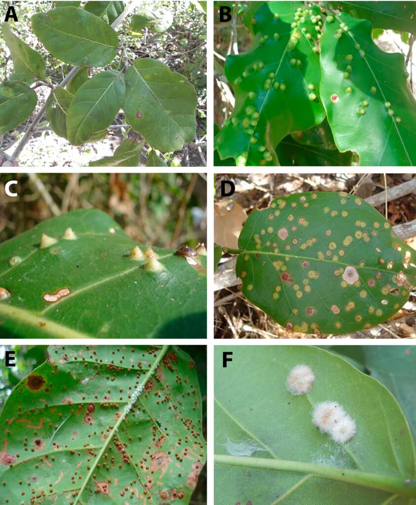
Figure 1. Leaf gall morphotypes found on Coccoloba barbadensis Jacq. (Polygonaceae). A) Leaves of C. barbadensis; B) capsule-shaped gall; C) conical gall; D) flattened gall; E) spherical gall; F) rounded gall.
A significant relationship (R2 = 0.731, F = 21.796, p < 0.001) between the average number of total galls collected during the sampled weeks was observed, with the presence of galls in the leaves gradually increasing throughout the weeks during the dry season. The number of galls was relatively constant during the first 4 weeks (March 25-29 to April 22-23), but from the fifth week (April 29-30) it gradually increased (Fig. 2A).
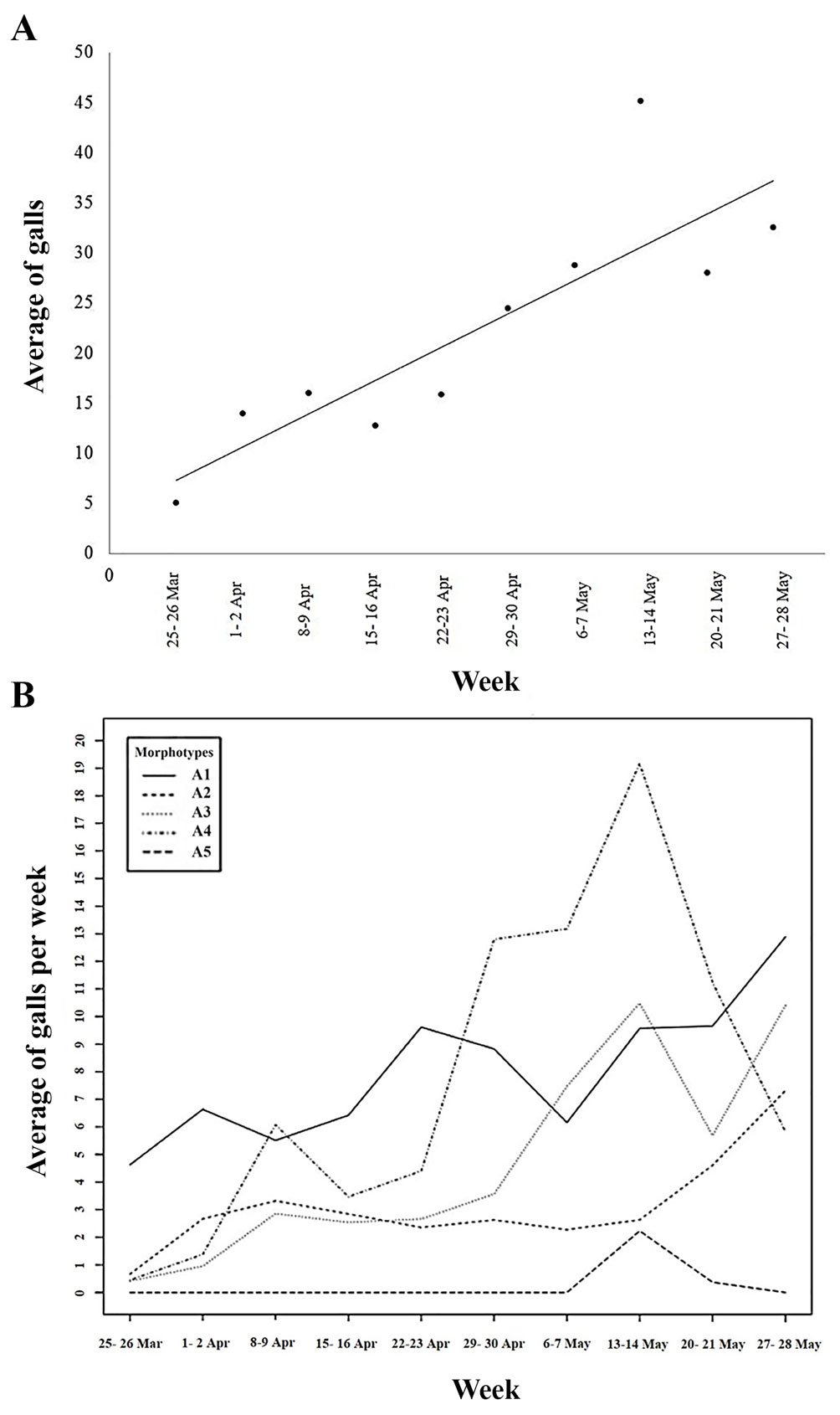
Figure 2. A) Simple linear regression showing the average number of collected leaf galls on C. barbadensis during the time of collect in the dry season; B) graphic showing the average number of each leaf gall morphotype during the time of collect in the dry season.
Most galls collected during the dry season corresponded to gall morphotypes 1 and 4 (35% and 32%, respectively) and were present in 87% and 80% of the examined trees, respectively. Cecidomyiid exuviates adhered to the latter 2 gall morphotypes during the first 2 sampling weeks (25-26th of March – 1-2nd of April) and the last week of February, respectively. On the other hand, 13%, 18.5%, and 1.5% of the remaining galls belonged to gall morphotypes 2, 3, and 5 and occurred in 73%, 80%, and 13% of the trees, respectively. During the rainy season, 17.5%, 26.4%, 30.7%, and 25.4% of the collected galls corresponded to morphotype galls 1 to 4, respectively.
The average number of each gall morphotype varied over time during the dry season. There were significant differences between each type of gall (F3,128 = 8.616, p < 0.001) (Fig. 2B). The frequency of gall morphotype 1 gradually increased during the first weeks, though by the last week of April they were no longer registered. In contrast, gall morphotype 2 showed a lower abundance but its number was relatively constant throughout the sampling period, whereas gall morphotypes 3 and 4 had a low frequency but their number increased towards the first week of May. Gall morphotype 5 was only observed during the last 2 sampling weeks.
Integrative taxonomy
A total of 2,008 larvae and 356 adult insects were obtained from the dissected galls during both seasons. The morphospecies including larvae, pupae, and adults were first discriminated, for which were subsequently generated 230 COI sequences (151 sequences of Hymenoptera, 77 of Diptera, 1 of Coleoptera, and 1 of Lepidoptera (GenBank accession numbers in Appendix) resulting in 125 haplotypes. The number of species per family delimited by the 2 DNA sequence-based species delimitation approaches is provided in Table 1. The 2% COI divergence criterion and the GMYC model discriminated between 34 and 38 species, respectively. The NJ distance tree derived from the examined COI sequences of Hymenoptera and Diptera is shown in figures 3 and 4, respectively. There were 2 inconsistencies between both approaches. The 2% COI divergence criterion delimited 1 species of Chrysonotomyia (Entedoninae: Eulophidae) and 2 of Teniupetiolus (Eurytominae: Eurytomidae), whereas the GMYC model divided them into 3 and 2 species, respectively.
DNA sequence data supported most of the delimited species using larvae and adults, except for the only species of Torymus Dalman (Hymenoptera: Torymidae), the 3 species of Cecidomyiidae (Diptera), and the single species of Lepidoptera and Coleoptera, for which we only generated sequences of larvae.
Insect-gall association
Gall morphotype 3 had the highest insect species richness (20 species), which comprised all sampled families except the hymenopteran species of Braconidae (Allorhogas coccolobae Martínez & Zaldívar-Riverón) and Torymidae (Torymus sp.). This gall morphotype also had the highest number of eulophid species (8), from which 5 belong to the subfamily Tetrastichinae and was only present in this gall morphotype. Gall morphotype 1 had 18 associated insect species, with Platygastridae and Eurytomidae (Hymenoptera) being the families with more species (5 and 4 species, respectively; Table 2). Gall morphotypes 2 and 4, on the other hand, registered 9 and 12 species, respectively, whereas gall morphotype 5 only had 4 species, 1 belonging to Eulohpidae (Hymenoptera), 1 to Platygastridae (Hymenoptera) and 2 to Cecidomyiidae (Diptera) (Table 2).
Larvae of Cecidomyiidae were highly abundant throughout the dry season. The abundance of larvae and adults of the families Eurytomidae and Braconidae, on the other hand, considerably increased towards the sixth week of the dry season. In contrast, the presence of immature stages of Eulophidae was more frequent at the beginning of the dry season, though adults were also observed throughout this sampling period. Platygastridae was the hymenopteran family that was most frequently found in both larval and adult stages. Only immature individuals of Cecidomyiidae (Diptera) and Eulophidae (Hymenoptera) were collected during the rainy season.
A statistically significant difference (c2 = 912,989, df = 102, p <0.001) was observed between the 4 morphotypes of galls recorded during the dry season and their associated insect species. Fourteen out of the 37 insect species delimited with 2% barcoding were associated with a single gall morphotype. These included a species of Tenuipetiolus (Eurytomidae) in gall morphotype 1, 5 of Tetrastichinae (Eulophidae) in gall morphotypes 3, 1 species of Chrysonotomyia (Eulophidae) in gall morphotypes 1, 2 and 3, respectively, the single species of Eupelmidae and Torymidae in gall morphotypes 1 and 4, respectively, 2 and 1 species of Platygastridae in gall morphotypes 1 and 3, respectively, and 1 species of Cecidomyiidae in gall morphotype 3. Five delimited species of Cecidomyiidae were recorded in gall morphotypes 3 and 4, whereas 4, 3, and 2 were present in gall morphotypes 2, 1, and 5, respectively.
Discussion
A considerable leaf gall diversity in C. barbadensis is recorded here. Based on the gathered information, the inducers of these 5 types of leaf galls were species of Cecidomyiidae (Diptera) (see below). Other cecidomyiid galls that have been reported on species of Coccoloba include those found on stems of C. mosenii Lindl., on leaves of Coccoloba cf. warmingii Meisn., C. diversifolia Jacq., C. swartzii Kuntze, and C. uvifera Meins., and on inflorescences of C. alnifolia Casar (Mead, 1970; Maia et al., 2008; Ramos-Rodrigues et al., 2014). The number of different types of galls found in C. barbadensis (5 morphotypes) is higher than those reported for the above species (≤ 2 morphotypes). However, based on their general appearance, the gall morphotypes 1 and 2 may be variants made by the same inducer species. Further rearing observations and molecular characterisation of gall inducers will help to confirm the actual gall diversity that is present on the leaves of this plant species.

Figure 3. Neighbour Joining phenogram reconstructed for specimens of Cecidomyiidae that were reared from the 4 leaf gall morphotypes found in C. barbadensis. Bars refer to the 7 species of Cecidomyiidae that were delimited with the 2% barcoding approach.
There is considerable morphological diversity in the leaf gall morphotypes found on C. barbadensis (Fig. 1A-F).
All these gall morphotypes were located on the leaf blade, with 4 of them being located on the beam and 1 on the underside. The considerable morphological diversity of these leaf galls can be attributed to several factors, among which include the high synthetic activity, rapid growth, structural and functional features, and characteristic morphogenetic patterns of leaf development (Mani, 1964). Further studies on these leaf galls are therefore necessary for a better understanding of the structural and histological differences among the leaf galls found on C. barbadensis.
Insect species richness
The high morphological diversity found on leaf galls favours the existence of a complex insect community (Mani, 1964); however, few studies have assessed in detail the insect community associated with leaf galls of Neotropical plant species (e.g., Maia, 2012). In this research, the extensive insect rearing, and examination of both molecular and morphological information helped to thoroughly characterise the insect species diversity found in the 5 types of galls present on leaves of C. barbadensis. Despite that, was not possible to confirm at this stage the biology of the reared taxa, and then their probable role is based on the relevant literature and the field observations.
Cecidomyiids, commonly known as gall midges, represent by far the group of insects with the most gall-inducer species (Gagné & Jaschhof, 2021). Species of Cecidomyiidae are mainly gall-formers, though members of the tribe Cecidomyiini are known to have a wide range of biologies, including only simple and complex gall formers, free-living, mycophagous, inquiline phytophagous, predator species of mites, aphids, and coccids, as well as internal parasitoids of aphids and psyllids (Kim et al., 2014; Uechi et al., 2011). The field observations and the insect species diversity found in the 5 leaf gall morphotypes of C. barbadensis strongly suggest that they are induced by cecidomyiid species. Among this evidence was that most of the dissected galls had a single cecidomyiid larva. Moreover, several galls belonging to morphotype 2 had a cecidomyiid pupal exuviae hanging outside of a small opening, which is a common feature of many galls with former cecidomyiids. Since the 5 leaf gall morphotypes were formed by cecidomyiid species, the remaining species of this family delimited in the study probably are inquilines.
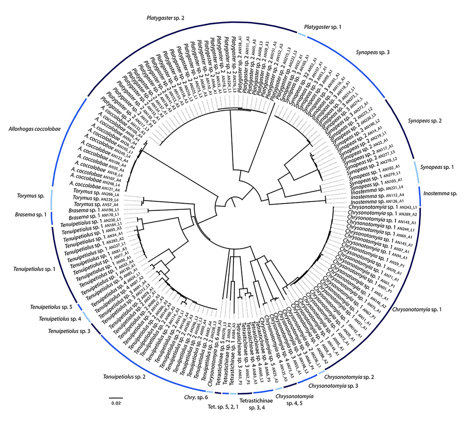
Figure 4. Neighbour Joining phenogram reconstructed for specimens of Hymenoptera that were reared from the 4 leaf gall morphotypes found in C. barbadensis. Bars refer to the 25 species of Hymenoptera that were delimited with the 2% barcoding approach.
The cecidomyiid larvae and their emerging adults could not be identified at the genus level; however, a BLAST similarity search of the barcoding locus for the delimited cecidomyiid species suggests that they are closely related to species of the Cecidomyiini genera Contarinia Geer and Macrodiplosis Kieffer. The gall-inducing species of the genus Contarinia are cosmopolitan and can be either monophagous or polyphagous with a wide range of hosts (Uechi et al., 2011). Most species of this genus live gregariously in the floral parts of the plant or in the galls that they induce on the leaves (Gagné & Jaschoff, 2021). Species of Macrodiplosis, on the other hand, are mainly gall inducers on leaves of plant species of the genus Quercus (Kim et al., 2014).
Table 1
Number of insect species discriminated by DNA sequence-based species delineation approaches conducted in this study (2% COI divergence criterion; GMYC method).
| Order/Family | Subfamily | Genus | 2% DC | GMYC |
| Diptera | ||||
| Cecidomyiidae | – | – | 7 | 7 |
| Lepidoptera | – | – | 1 | – |
| Coleoptera | – | – | 1 | – |
| Hymenoptera | ||||
| Braconidae | Doryctinae | Allorhogas coccolobae | 1 | 1 |
| Eulophidae | Entedoninae | Chrysonotomyia spp. | 6 | 8 |
| Tetrastichinae | Quadrastichus spp. | 5 | 5 | |
| Eupelmidae | Brasema sp. | 1 | 1 | |
| Eurytomidae | Eurytominae | Tenuipetiolus spp. | 5 | 7 |
| Platygastridae | Synopeas spp. | 3 | 3 | |
| Inostemma spp. | 1 | 1 | ||
| Undetermined | 2 | 2 | ||
| Torymidae | Torymus sp. | 1 | 1 | |
| Total | 34 | 38 |
Table 2
Insect species richness by order and family associated with 5 gall morphotypes found on leaves of Coocoloba barbadensis Jacq.
| Gall morphotypes (GM) | ||||||
| Insect Order/Family | GM 1 | GM 2 | GM 3 | GM 4 | GM 5 | TOTAL |
| Coleoptera | – | – | 1 | – | – | 1 |
| Lepidoptera | – | – | 1 | – | – | 1 |
| Diptera | ||||||
| Cecidomyiidae | 3 | 4 | 5 | 5 | 2 | 19 |
| Hymenoptera | 15 | 5 | 13 | 7 | 2 | 42 |
| Eurytomidae | 4 | 2 | 3 | 3 | – | 12 |
| Eulophidae | 3 | 2 | 8 | 1 | 1 | 15 |
| Eupelmidae | 1 | – | – | – | – | 1 |
| Braconidae | 1 | – | – | 1 | – | 2 |
| Platygastridae | 5 | 1 | 2 | 2 | 1 | 11 |
| Torymidae | 1 | – | – | – | – | 1 |
| Total | 18 | 9 | 20 | 12 | 4 | 63 |
Currently, 4 gall midge species are known to be associated with species of Coccoloba. The genus Ctenodactylomyia Felt (supertribe Cecidomyiidi, unplaced tribe) has 2 leaf gall inducer species on C. diversifolia Jacq., C. swartzii, and C. uvifera L. from the Caribbean (Gagné & Jaschoff, 2021). Moreover, Marilasioptera tripartite Möhn and Meunieriella magdalenae Wünsch (supertribe Lasiopteridi, tribe Alycaulini) were described as inquilines on galls induced by other insects on species of Coccoloba from El Salvador and Colombia, respectively (Gagné & Jaschoff, 2021). The present study increases the number of gall midge species associated with Coccoloba to 11.
Our study also found a considerable number of hymenopteran species reared from the 5 examined leaf gall morphotypes, most of which probably are parasitoids of the cecidomyiid species. These parasitoid species belong to the wasp families Eulophidae, Eupelmidae, Platygastridae, and Torymidae, whereas the only reared braconid species probably are phytophagous inquiline. Some members of the Platygastridae are known to be koinobiont endoparasitoids of gallery cecidomyiid eggs, and they are known to be closely associated with the parts of the plant where the host gall is found (Masner & Huggert, 1989; Masner, 1993). Eulophidae are also mainly parasitoids of holometabolous insect larvae (though in some cases also of eggs, prepupae, and pupae) of Lepidoptera, Hymenoptera, Diptera, and Coleoptera (Graham, 1991); however, some species have been reported to be phytophagous or predators (Gibson, 1993). Finally, members of the eupelmid subfamily Eupelminae, from which the genus Brasema belongs, mainly are parasitoids of larval stages of various insect hosts (Gibson, 1993).
The wasp family Eurytomidae is represented by entomophagous species that parasitise larval or pupal stages of Coleoptera, Diptera, and Hymenoptera as solitary endoparasitic idiobionts, though some species can be phytophagous feeding on seeds, or inquilines feeding on both their host and gall tissue (Lotfalizadeh et al., 2007; Gates & Delvare, 2008). Species of Tenuipetiolus have been reported to be parasitoids of gall inducer insects, including cecidomyiids and cynipids (Gates & Hanson, 2006; Zhang et al., 2014). Similarly, several species of Torymidae are known to be ectoparasitoids of gall-forming insects of the latter 2 families (Gibson, 1993).
The braconid species A. coccolobae (Doryctinae) was described a decade ago from the Chamela region in Jalisco, Mexico, based on specimens reared from leaf galls of C. barbadensis (Martínez & Zaldívar-Riverón, 2013), that correspond to the morphotype 2. Here, this braconid species was reared not only from the above leaf gall morphotype but also from morphotype 4. Several species of Allorhogas have been confirmed to feed on various plant families either by being gall formers or inquilines of galls made by other insect taxa (Centrella & Shaw, 2010; Chavarría et al., 2009; de Mâcedo et al., 1998; Zaldívar-Riverón et al., 2014). Since none of the Allorhogas species with recorded biology are known to be parasitoids, and due to the low abundance of this species compared with the cecidomyiid species that were reared from the same gall morphotypes, it is presumed that it could be a phytophagous inquiline.
The considerably high, mostly undescribed species diversity of cecidomyiid dipterans and parasitoid hymenopterans that we reared from the 5 leaf gall morphotypes of C. barbadensis remark the necessity to carry out more studies that focus on the species diversity of galls, particularly in tropical regions. Moreover, this study highlights the importance of performing integrative species delineation studies of insects present in galls to have a more accurate knowledge of their actual diversity and trophic interactions.
Acknowledgments
We thank L. Márquez, N. López, and A. Jiménez for their assistance in the laboratory (Lanabio), and Cristina Mayorga for her assistance at the CNIN-IBUNAM. Angélica Rodríguez was supported by a MSc scholarship given by the Consejo Nacional de Humanidades, Ciencias y Tecnologías (Conahcyt, Mexico), and she thanks the Posgrado en Ciencias Biológicas, UNAM, for support during her MSc studies. This study was finished thanks to the grants given by UNAM-DGAPA (PAPIIT Convocatoria 2022, Project IN201622), and Conahcyt, Mexico (Convocatoria Ciencia de Frontera, project number 58548) to AZR.
| Appendix. Continued. | ||||
| Order (Insecta) | Family, Genus | Species | DNA voucher No. | Genbank accession No. |
| Diptera | Cecidomyiidae | sp. | CeciAN255_L2 | PP659768 |
| Diptera | Cecidomyiidae | sp. | CeciAN23_L2 | PP659794 |
| Diptera | Cecidomyiidae | sp. | CeciAN193_L2 | PP659795 |
| Diptera | Cecidomyiidae | sp. | CeciAN291_A3 | PP659802 |
| Diptera | Cecidomyiidae | sp. | CeciAN292_A1 | PP659803 |
| Diptera | Cecidomyiidae | sp. | CeciAN257_L2 | PP659804 |
| Diptera | Cecidomyiidae | sp. | CeciAN259_L3 | PP659805 |
| Diptera | Cecidomyiidae | sp. | CeciAN262_L4 | PP659806 |
| Diptera | Cecidomyiidae | sp. | CeciAN207_L4 | PP659797 |
| Diptera | Cecidomyiidae | sp. | CeciAN290_A1 | PP659801 |
| Diptera | Cecidomyiidae | sp. | CeciAN160_L3 | PP659807 |
| Diptera | Cecidomyiidae | sp. | CeciAN02_L4 | PP659731 |
| Diptera | Cecidomyiidae | sp. | CeciAN05_L4 | PP659732 |
| Diptera | Cecidomyiidae | sp. | CeciAN159_L1 | PP659733 |
| Diptera | Cecidomyiidae | sp. | CeciAN165_L2 | PP659734 |
| Diptera | Cecidomyiidae | sp. | CeciAN166_L2 | PP659735 |
| Diptera | Cecidomyiidae | sp. | CeciAN167_L3 | PP659736 |
| Diptera | Cecidomyiidae | sp. | CeciAN168_L4 | PP659737 |
| Diptera | Cecidomyiidae | sp. | CeciAN169_L4 | PP659738 |
| Diptera | Cecidomyiidae | sp. | CeciAN171_L1 | PP659739 |
| Diptera | Cecidomyiidae | sp. | CeciAN173_L1 | PP659740 |
| Diptera | Cecidomyiidae | sp. | CeciAN176_L1 | PP659741 |
| Diptera | Cecidomyiidae | sp. | CeciAN180_L2 | PP659742 |
| Diptera | Cecidomyiidae | sp. | CeciAN183_L1 | PP659743 |
| Diptera | Cecidomyiidae | sp. | CeciAN186_L5 | PP659744 |
| Diptera | Cecidomyiidae | sp. | CeciAN188_L1 | PP659745 |
| Diptera | Cecidomyiidae | sp. | CeciAN191_L1 | PP659747 |
| Diptera | Cecidomyiidae | sp. | CeciAN231_L1 | PP659750 |
| Diptera | Cecidomyiidae | sp. | CeciAN233_L1 | PP659751 |
| Diptera | Cecidomyiidae | sp. | CeciAN234_L2 | PP659752 |
| Diptera | Cecidomyiidae | sp. | CeciAN237_L1 | PP659753 |
| Diptera | Cecidomyiidae | sp. | CeciAN245_L1 | PP659755 |
| Diptera | Cecidomyiidae | sp. | CeciAN267_L1 | PP659756 |
| Diptera | Cecidomyiidae | sp. | CeciAN06_A3 | PP659791 |
| Diptera | Cecidomyiidae | sp. | CeciAN209_L5 | PP659749 |
| Diptera | Cecidomyiidae | sp. | CeciAN43_A2 | PP659792 |
| Diptera | Cecidomyiidae | sp. | CeciAN189_L3 | PP659746 |
| Diptera | Cecidomyiidae | sp. | CeciAN194_L3 | PP659748 |
| Diptera | Cecidomyiidae | sp. | CeciAN239_L4 | PP659754 |
| Hymenoptera | Platygaster | sp. | TeleAN08_L3 | PP481223 |
| Hymenoptera | Platygaster | sp. | TeleAN19_P3 | PP481224 |
| Hymenoptera | Platygaster | sp. | TeleAN46_A1 | PP481225 |
| Hymenoptera | Platygaster | sp. | TeleAN45_A3 | PP481226 |
| Hymenoptera | Platygaster | sp. | TeleAN50_A3 | PP481227 |
| Hymenoptera | Platygaster | sp. | TeleAN30_A3 | PP481228 |
| Hymenoptera | Platygaster | sp. | TeleAN132_A3 | PP481229 |
| Hymenoptera | Platygaster | sp. | TeleAN133_A1 | PP481230 |
| Hymenoptera | Platygaster | sp. | TeleAN134_A3 | PP481231 |
| Hymenoptera | Platygaster | sp. | TeleAN135_A1 | PP481232 |
| Hymenoptera | Platygaster | sp. | TeleAN137_A1 | PP481233 |
| Hymenoptera | Platygaster | sp. | TeleAN138_A3 | PP481234 |
| Hymenoptera | Platygaster | sp. | TeleAN141_A3 | PP481235 |
| Hymenoptera | Platygaster | sp. | TeleAN151_A3 | PP481236 |
| Hymenoptera | Platygaster | sp. | TeleAN152_A3 | PP481237 |
| Hymenoptera | Platygaster | sp. | TeleAN153_A3 | PP481238 |
| Hymenoptera | Platygaster | sp. | TeleAN154_A3 | PP481239 |
| Hymenoptera | Platygaster | sp. | TeleAN156_A3 | PP481240 |
| Hymenoptera | Platygaster | sp. | TeleAN215_L3 | PP481241 |
| Hymenoptera | Platygaster | sp. | TeleAN216_L3 | PP481242 |
| Hymenoptera | Platygaster | sp. | TeleAN217_L3 | PP481243 |
| Hymenoptera | Platygaster | sp. | TeleAN218_L3 | PP481244 |
| Hymenoptera | Platygaster | sp. | TeleAN224_L1 | PP481245 |
| Hymenoptera | Platygaster | sp. | TeleAN225_L1 | PP481246 |
| Hymenoptera | Platygaster | sp. | TeleAN275_L3 | PP481247 |
| Hymenoptera | Platygaster | sp. | TeleAN276_L3 | PP481248 |
| Hymenoptera | Platygaster | sp. | TeleAN281_A3 | PP481249 |
| Hymenoptera | Platygaster | sp. | TeleAN158_A1 | PP481250 |
| Hymenoptera | Platygaster | sp. | TeleAN110_A1 | PP481251 |
| Hymenoptera | Platygaster | sp. | TeleAN111_A3 | PP481252 |
| Hymenoptera | Synopeas | sp. | PlatyAN22_A1 | PP481253 |
| Hymenoptera | Synopeas | sp. | PlatyAN32_A1 | PP481254 |
| Hymenoptera | Synopeas | sp. | PlatyAN52_A1 | PP481255 |
| Hymenoptera | Synopeas | sp. | PlatyAN14_A1 | PP481256 |
| Hymenoptera | Synopeas | sp. | PlatyAN157_A1 | PP481257 |
| Hymenoptera | Synopeas | sp. | PlatyAN53_A1 | PP481258 |
| Hymenoptera | Synopeas | sp. | PlatyAN99_A1 | PP481259 |
| Hymenoptera | Synopeas | sp. | PlatyAN101_A1 | PP481260 |
| Hymenoptera | Synopeas | sp. | PlatyAN102_A1 | PP481261 |
| Hymenoptera | Synopeas | sp. | PlatyAN103_A1 | PP481262 |
| Hymenoptera | Synopeas | sp. | PlatyAN105_A1 | PP481263 |
| Hymenoptera | Synopeas | sp. | PlatyAN190_L2 | PP481264 |
| Hymenoptera | Synopeas | sp. | PlatyAN219_L1 | PP481265 |
| Hymenoptera | Inostemma | sp. | PlatyAN221_L4 | PP481266 |
| Hymenoptera | Synopeas | sp. | PlatyAN223_L2 | PP481267 |
| Hymenoptera | Synopeas | sp. | PlatyAN220_L5 | PP481268 |
| Hymenoptera | Inostemma | sp. | PlatyAN112_A4 | PP481269 |
| Hymenoptera | Synopeas | sp. | PlatyAN116_A1 | PP481270 |
| Hymenoptera | Synopeas | sp. | PlatyAN117_A1 | PP481271 |
| Hymenoptera | Synopeas | sp. | PlatyAN118_A1 | PP481272 |
| Hymenoptera | Inostemma | sp. | PlatyAN126_A1 | PP481273 |
| Hymenoptera | Synopeas | sp. | PlatyAN214_L1 | PP481274 |
| Hymenoptera | Platygaster | sp. | PlatyAN222_L3 | PP481275 |
| Hymenoptera | Synopeas | sp. | PlatyAN272_A1 | PP481276 |
| Hymenoptera | Synopeas | sp. | PlatyAN273_L | PP481277 |
| Hymenoptera | Synopeas | sp. | PlatyAN274_L | PP481278 |
| Hymenoptera | Synopeas | sp. | PlatyAN277_L5 | PP481279 |
| Hymenoptera | Synopeas | sp. | PlatyAN278_L2 | PP481280 |
| Hymenoptera | Synopeas | sp. | PlatyAN279_L1 | PP481281 |
| Hymenoptera | Tenuipetiolus | sp. | EurytAN96_A1 | PP481282 |
| Hymenoptera | Tenuipetiolus | sp. | EurytAN265_L3 | PP481283 |
| Hymenoptera | Chrysonotomyia | sp. | EntedAN01_P1 | PP481284 |
| Hymenoptera | Chrysonotomyia | sp. | EntedAN07_A1 | PP481285 |
| Hymenoptera | Chrysonotomyia | sp. | EntedAN29_A1 | PP481286 |
| Hymenoptera | Chrysonotomyia | sp. | EntedAN11_A1 | PP481287 |
| Hymenoptera | Chrysonotomyia | sp. | EntedAN31_A1 | PP481288 |
| Hymenoptera | Chrysonotomyia | sp. | EntedAN51_A1 | PP481289 |
| Hymenoptera | Chrysonotomyia | sp. | EntedAN59_P1 | PP481290 |
| Hymenoptera | Chrysonotomyia | sp. | EntedAN61_P1 | PP481291 |
| Hymenoptera | Chrysonotomyia | sp. | EntedAN67_P1 | PP481292 |
| Hymenoptera | Chrysonotomyia | sp. | EntedAN69_A1 | PP481293 |
| Hymenoptera | Chrysonotomyia | sp. | EntedAN70_A1 | PP481294 |
| Hymenoptera | Chrysonotomyia | sp. | EntedAN71_A1 | PP481295 |
| Hymenoptera | Chrysonotomyia | sp. | EntedAN72_A1 | PP481296 |
| Hymenoptera | Chrysonotomyia | sp. | EntedAN75_A1 | PP481297 |
| Hymenoptera | Chrysonotomyia | sp. | EntedAN94_A1 | PP481298 |
| Hymenoptera | Chrysonotomyia | sp. | EntedAN95_A1 | PP481299 |
| Hymenoptera | Chrysonotomyia | sp. | EntedAN25_A2 | PP481300 |
| Hymenoptera | Chrysonotomyia | sp. | EntedAN64_P4 | PP481301 |
| Hymenoptera | Chrysonotomyia | sp. | EntedAN73_A3 | PP481302 |
| Hymenoptera | Chrysonotomyia | sp. | EntedAN142_A1 | PP481303 |
| Hymenoptera | Chrysonotomyia | sp. | EntedAN143_A1 | PP481304 |
| Hymenoptera | Chrysonotomyia | sp. | EntedAN144_A1 | PP481305 |
| Hymenoptera | Chrysonotomyia | sp. | EntedAN145_A1 | PP481306 |
| Hymenoptera | Chrysonotomyia | sp. | EntedAN146_A2 | PP481307 |
| Hymenoptera | Chrysonotomyia | sp. | EntedAN198_L3 | PP481308 |
| Hymenoptera | Chrysonotomyia | sp. | EntedAN236_L1 | PP481309 |
| Hymenoptera | Chrysonotomyia | sp. | EntedAN243_L1 | PP481310 |
| Hymenoptera | Chrysonotomyia | sp. | EntedAN244_L1 | PP481311 |
| Hymenoptera | Chrysonotomyia | sp. | EntedAN288_A2 | PP481312 |
| Hymenoptera | Chrysonotomyia | sp. | EntedAN289_A2 | PP481313 |
| Hymenoptera | Chrysonotomyia | sp. | EntedAN58_P1 | PP481314 |
| Hymenoptera | Chrysonotomyia | sp. | EntedAN55_A1 | PP481315 |
| Hymenoptera | Chrysonotomyia | sp. | EulopAN125_A5 | PP481316 |
| Hymenoptera | Tetrastichinae | sp. | TetrasAN84_A3 | PP481317 |
| Hymenoptera | Tetrastichinae | sp. | TetrasAN62_P3 | PP481318 |
| Hymenoptera | Tetrastichinae | sp. | TetrasAN63_P3 | PP481319 |
| Hymenoptera | Tetrastichinae | sp. | TetrasAN66_P3 | PP481320 |
| Hymenoptera | Tetrastichinae | sp. | TetrasAN83_A3 | PP481321 |
| Hymenoptera | Tetrastichinae | sp. | TetrasAN60_P3 | PP481322 |
| Hymenoptera | Tetrastichinae | sp. | TetrasAN269_L3 | PP481323 |
| Hymenoptera | Tetrastichinae | sp. | TetrasAN270_L3 | PP481324 |
| Hymenoptera | Tenuipetiolus | sp. | EurytAN77_A1 | PP481325 |
| Hymenoptera | Tenuipetiolus | sp. | EurytAN81_A3 | PP481326 |
| Hymenoptera | Tenuipetiolus | sp. | EurytAN93_A3 | PP481327 |
| Hymenoptera | Allorhogas | coccolobae | AllorAN18_L4 | PP481328 |
| Hymenoptera | Allorhogas | coccolobae | AllorAN28_A4 | PP481329 |
| Hymenoptera | Allorhogas | coccolobae | AllorAN35_A4 | PP481330 |
| Hymenoptera | Allorhogas | coccolobae | AllorAN48_A4 | PP481331 |
| Hymenoptera | Allorhogas | coccolobae | AllorAN56_A4 | PP481332 |
| Hymenoptera | Allorhogas | coccolobae | AllorAN107_A4 | PP481333 |
| Hymenoptera | Allorhogas | coccolobae | AllorAN108_A4 | PP481334 |
| Hymenoptera | Allorhogas | coccolobae | AllorAN109_A4 | PP481335 |
| Hymenoptera | Allorhogas | coccolobae | AllorAN121_A4 | PP481336 |
| Hymenoptera | Allorhogas | coccolobae | AllorAN122_A4 | PP481337 |
| Hymenoptera | Allorhogas | coccolobae | AllorAN195_L1 | PP481338 |
| Hymenoptera | Allorhogas | coccolobae | AllorAN248_L4 | PP481339 |
| Hymenoptera | Allorhogas | coccolobae | AllorAN249_L4 | PP481340 |
| Hymenoptera | Tenuipetiolus | sp. | EurytAN212_L3 | PP481341 |
| Hymenoptera | Tenuipetiolus | sp. | EurytAN228_L3 | PP481342 |
| Hymenoptera | Tenuipetiolus | sp. | EurytAN246_L3 | PP481343 |
| Hymenoptera | Tenuipetiolus | sp. | EurytAN285_A3 | PP481344 |
| Hymenoptera | Tenuipetiolus | sp. | EurytAN286_A3 | PP481345 |
| Hymenoptera | Tenuipetiolus | sp. | EurytAN37_A1 | PP481346 |
| Hymenoptera | Tenuipetiolus | sp. | EurytAN147_A3 | PP481347 |
| Hymenoptera | Tenuipetiolus | sp. | EurytAN148_A4 | PP481348 |
| Hymenoptera | Tenuipetiolus | sp. | EurytAN149_A3 | PP481349 |
| Hymenoptera | Tenuipetiolus | sp. | EurytAN130_A1 | PP481350 |
| Hymenoptera | Tenuipetiolus | sp. | EurytAN87_A2 | PP481351 |
| Hymenoptera | Tenuipetiolus | sp. | EurytAN91_A4 | PP481352 |
| Hymenoptera | Tenuipetiolus | sp. | EurytAN80_A3 | PP481353 |
| Hymenoptera | Tenuipetiolus | sp. | EurytAN82_A4 | PP481354 |
| Hymenoptera | Tenuipetiolus | sp. | EurytAN90_A4 | PP481355 |
| Hymenoptera | Tenuipetiolus | sp. | EurytAN85_A1 | PP481356 |
| Hymenoptera | Torymus | sp. | EurytAN57_A4 | PP481357 |
| Hymenoptera | Tenuipetiolus | sp. | EurytAN164_L1 | PP481358 |
| Hymenoptera | Tenuipetiolus | sp. | EurytAN227_L1 | PP481359 |
| Hymenoptera | Tenuipetiolus | sp. | EurytAN230_L1 | PP481360 |
| Hymenoptera | Tenuipetiolus | sp. | EurytAN283_A2 | PP481361 |
| Hymenoptera | Tenuipetiolus | sp. | EurytAN33_A4 | PP481362 |
| Hymenoptera | Tenuipetiolus | sp. | EurytAN34_A1 | PP481363 |
| Hymenoptera | Tenuipetiolus | sp. | EurytAN15_L1 | PP481364 |
| Hymenoptera | Tenuipetiolus | sp. | EurytAN114_A3 | PP481365 |
| Hymenoptera | Tenuipetiolus | sp. | EurytAN79_A1 | PP481366 |
| Hymenoptera | Tenuipetiolus | sp. | EurytAN78_A1 | PP481367 |
| Hymenoptera | Tenuipetiolus | sp. | EurytAN24_L1 | PP481368 |
| Hymenoptera | Chrysonotomyia | sp. | EurytAN88_A3 | PP481369 |
| Hymenoptera | Brasema | sp. | ToryAN170_L1 | PP481370 |
| Hymenoptera | Brasema | sp. | ToryAN196_L1 | PP481371 |
| Hymenoptera | Torymus | sp. | EurytAN229_L4 | PP481372 |
| Hymenoptera | Torymus | sp. | EurytAN266_L4 | PP481373 |
| Coleoptera | AN184 | PP897664 | ||
| Lepidoptera | AN250_L3 | PP897665 |
References
Altschul, S. F., Gish, W., Miller, W., Myers, E. W., & Lipman, D. J. (1990). Basic local alignment search tool. Journal of Molecular Biology, 215, 403–410. https://doi.org/10.1016/S0022-2836(05)80360-2
Bortolus, A. (2008). Error cascades in the biological sciences: the unwanted consequences of using bad taxonomy in ecology. AMBIO: A Journal of the Human Environment, 37, 114–118. https://doi.org/10.1579/0044-7447(2008)37[114:ECITBS]2.0.CO;2
Bouckaert, R., Heled, J., Kühnert, D., Vaughan, T., Wu, C. H., Xie, D., Suchard, M. A., Rambaut, A., & Drummond, A. J. (2014). BEAST 2: A software platform for Bayesian evolutionary analysis. Plos Computational Biology, 10, e1003537. https://doi.org/10.1371/journal.pcbi.1003537
Centrella, M. L., & Shaw, S. R. (2010). A new species of phytophagous braconid Allorhogas minimus (Hymenoptera: Braconidae: Doryctinae) reared from fruit galls on Miconia longifolia (Melastomataceae) in Costa Rica. International Journal of Tropical Insect Science, 30, 101–107. https://doi.org/10.1017/S1742758410000147
Chavarría, L., Hanson, P., Marsh, P., & Shaw, S. (2009). A phytophagous braconid, Allorhogas conostegia sp. nov.(Hymenoptera: Braconidae), in the fruits of Conostegia xalapensis (Bonpl.) D. Don (Melastomataceae). Journal of Natural History, 43, 2677–2689. https://doi.org/10.1080/
00222930903243996
Clare, E. L., Schiestl, F. P., Leitch, A. R., & Chittka, L. (2013). The promise of genomics in the study of plant-pollinator interactions. Genome Biology, 14, 1–11. https://doi.org/10.
1186/gb-2013-14-6-207
de Macêdo, M. V., & Monteiro, R. F. (1989). Seed predation by a braconid wasp, Allorhogas sp. (Hymenoptera). Journal of the New York Entomological Society, 97, 358–362.
Dexter, K. G., Pennington, T. D., & Cunningham, C. W. (2010). Using DNA to assess errors in tropical tree identifications: How often are ecologists wrong and when does it matter? Ecological Monographs, 80, 267–286. https://doi.org/10.1890/09-0267.1
Drummond, A. J., Suchard, M. A., Xie, D., & Rambaut, A. (2012). Bayesian phylogenetics with BEAUti and the BEAST 1.7. Molecular Biology and Evolution, 29, 1969–1973. https://doi.org/10.1093/molbev/mss075
Folmer O., Black, M., Hoeh, W., Lutz, R., & Vrijenhoek, R. (1994). DNA primers for amplification of mitochondrial cytochrome c oxidase subunit I from diverse metazoan invertebrates. Molecular Marine Biology and Biotechnology, 3, 294–299.
Forbes, A. A., Hall, M. C., Lund, J., Hood, G. R., Izen, R., Egan, S. P. et al. (2016). Parasitoids, hyperparasitoids, and inquilines associated with the sexual and asexual generations of the gall former, Belonocnema treatae (Hymenoptera: Cynipidae). Annals of the Entomological Society of America, 109, 49–63. https://doi.org/10.1093/aesa/sav112
Gagné, R. J., & Jaschhof, M. (2021). A catalog of the
Cecidomyiidae (Diptera) of the World, 5th Edition. Available
at: https://www.ars.usda.gov/ARSUserFiles/80420580/Gag
ne_Jaschhof_2021_World_Cat_5th_Ed.pdf
Gates, M. W., & Hanson, P. E. (2006). Familia Eurytomidae, In P. E. Hanson, & I. D. Gauld (Eds.), Hymenoptera de la region tropical (pp. 380–387). Memoirs of the American Entomological Institute, 77, 1–994.
Gates, M., & Delvare, G. (2008). A new species of Eurytoma (Hymenoptera: Eurytomidae) attacking Quadrastichus spp. (Hymenoptera: Eulophidae) galling Erythrina spp. (Fabaceae), with a summary of African Eurytoma biology and species checklist. Zootaxa, 1751, 1–24. https://doi.org/10.11646/zootaxa.1751.1.1
Gibson, L. (1993). Superfamilies Mymarommatoidea and Chalcidoidea. In H. Goulet, & J. T. Huber (Eds.), Hymenoptera of the world: an identification guide to families (pp.570–655). Research Branch, Agriculture, Canada, Publication 1894.
Graham, M. W. R. V. (1991). A reclassification of the European Tetrastichinae (Hymenoptera: Eulophidae). Revision of the remaining genera. Memoirs of the American Entomological Institute, 49, 1–322.
Hebert, P. D., Cywinska, A., Ball, S. L., & DeWaard, J R. (2003). Biological identifications through DNA barcodes. Proceedings of the Royal Society of London. Series B: Biological Sciences, 2070, 313–321. https://doi.org/10.1098/rspb.2002.2218
Hebert, P. D., Penton, E. H., Burns, J. M., Janzen, H. D., & Hallwachs, W. (2004). Ten species in one: DNA barcoding reveals cryptic species in the Neotropical skipper butterfly Astrapes fulgerator. Proceeding of the National Academy of Sciences, 101, 14812–14817. https://doi.org/10.1073/pnas.
0406166101
Howard, R. A. (1959). Studies in the genus Coccoloba. VII A synopsis and key to species in Mexico and Central America. Journal of the Arnold Arboretum, 40, 176–203.
Ings, T. C., Montoya, J. M., Bascompte, J., Blüthgen, N., Brown, L., Dormann, C. F. et al. (2009). Ecological networks-beyond food webs. Journal of Animal Ecology, 78, 253–269. https://doi.org/10.1111/j.1365-2656.2008.01460.x
Kaartinen, R., Stone, G. N., Hearn, J., Lohse, K., & Roslin, T. (2010). Revealing secret liaisons: DNA barcoding changes our understanding of food webs. Ecological Entomology, 35, 623–638. https://doi.org/10.1111/j.1365-2311.2010.01224.x
Kaartinen, R., & Roslin, T. (2011). Shrinking by numbers: landscape context affects the species composition but not the quantitative structure of local food webs. Journal of Animal Ecology, 80, 622–631. https://doi.org/10.1111/
j.1365-2656.2011.01811.x
Kim, W., Yukawa, J., Harris, K. M., Minami, T., Matsuo, K., & Skrzypczyńska, M. (2014). Description, host range, and distribution of a new Macrodiplosis species (Diptera: Cecidomyiidae) that induces leaf-margin fold galls on deciduous Quercus (Fagaceae) with comparative notes on Palaearctic congeners. Zootaxa, 3821, 222–238. https://doi.org/10.11646/zootaxa.3821.2.3
Lotfalizadeh, H., Delvare, G., & Rasplus, J. Y. (2007). Phylogenetic analysis of Eurytominae (Chalcidoidea: Eurytomidae) based on morphological characters. Zoological Journal of the Linnean Society, 151, 441–510. https://doi.org/10.1111/j.1096-3642.2007.00308.x
Maia, V. C., Magenta, M. A. G., & Martins, S. E. (2008). Ocorrência e caracterização de galhas de insetos em áreas de restinga de Bertioga (São Paulo, Brasil). Biota Neotropica, 8, 167–197. https://doi.org/10.1590/S1676-06032
008000100020
Maia, V. C. (2012). Richness of hymenopterous galls from South America. Papéis Avulsos de Zoologia, 52, 423–429. https://doi.org/10.1590/S0031-10492012021500001
Mani, M. S. (1964). Ecology of plant galls. The Hague: W. Junk.
Martínez, J. J., & Zaldívar-Riverón, A. (2013). Seven new species of Allorhogas (Hymenoptera: Braconidae: Doryctinae) from Mexico. Revista Mexicana de Biodiversidad, 84, 117–139. https://doi.org/10.7550/rmb.31955
Masner, L., & Huggert, L. (1989). World review and keys to genera of the subfamily Inostemmatinae with the reassignment of the taxa to the Platygastrinae and Sceliotrachelinae (Hymenoptera: Platygastridae). The Memoirs of the Entomological Society of Canada, 121, 3–216.
Masner, L. (1993). Superfamily Platygastroidea. In H. Goulet, & J. T. Huber (Eds.), Hymenoptera of the world: an identification guide to families (pp.558–565). Research Branch, Agriculture, Canada, Publication 1894.
Mead, F. W. (1970). Ctenodactylomyia watsoni Felt, a gall midge of seagrape, Coccoloba uvifera L. Florida (Diptera: Cecidomyiidae). Entomology Circular, 97. Florida Department of Agriculture & Consumer Services Division of Plant Industry. Florida, USA.
Méndez-Alonzo, R., Pineda-García, F., Paz, H., Rosell, J. A., & Olson, M. E. (2013). Leaf phenology is associated with soil water availability and xylem traits in a tropical dry forest. Trees, 27, 745–754. https://doi.org/10.1007/s00468-012-0829-x
Nieves-Aldrey, J. L. (1998). Insectos que inducen la formación de agallas en las plantas: Una fascinante interacción ecológica y evolutiva. Boletín de la Sociedad Entomológica Aragonesa, 23, 3–12.
Noguera, F. A., Vega-Rivera, J. H., García-Aldrete, A. N., Quesada-Avendaño, M. (Eds.). (2002). Historia natural de Chamela. Mexico City: Universidad Nacional Autónoma de México.
Paine, R. T. (1980). Food webs: linkage, interaction strength, and community infrastructure. Journal of Animal Ecology, 49, 667–685. https://doi.org/10.2307/4220
Pons, J., Barraclough, T. G., Gomez-Zurita, J., Cardoso, A., Duran, D. P., Hazell, S., Kamoun, S., Sumlin, W. D., & Vogler, A. P. (2006). Sequence-based species delimitation for the DNA taxonomy of undescribed insects. Systematic Biology, 55, 595-609. https://doi.org/10.1080/10635150600852011
Posada, D. (2004). Collapse: describing haplotypes from sequence alignments. Vigo, Spain: University of Vigo. https://dposada.webs.uvigo.es/
Price, P. W. (2005). Adaptive radiation of gall-inducing insects. Basic and Applied Ecology, 6, 413–421. https://doi.org/10.1016/j.baae.2005.07.002
Prosser, S., Martínez-Arce, A., & Elías-Gutiérrez, M. (2013). A new set of primers for COI amplification from freshwater microcrustaceans. Molecular Ecology Resources, 13, 1151–1155. https://doi.org/10.1111/1755-0998.12132
R Core Team (2021). R: A language and environment for statistical computing. R Foundation for statistical computing, Vienna, Austria. http://r-forge.r-project.org/projects/splits/
Raman, A., & Withers, T. M. (2003). Oviposition by introduced Ophelimus eucalypti (Hymenoptera: Eulophidae) and morphogenesis of female-induced galls on Eucalyptus saligna (Myrtaceae) in New Zealand. Bulletin of Entomological Research, 93, 55–63. https://doi.org/10.1079/BER2002217
Raman, A. (2011). Morphogenesis of insect-induced plant galls facts and questions. Flora-Morphology, Distribution, Functional Ecology of Plants, 206, 517–533. https://doi.org/10.1016/j.flora.2010.08.004
Ratnasingham, S., & Hebert, P. D. N. (2013). A DNA-based registry for all animal species: the barcode index number (BIN) system. Plos One, 8, e66213. https://doi.org/10.1371/journal.pone.0066213
Razo-González, M., Castano-Meneses, G., Callejas-Chavero, A., Pérez-Velázquez, D., & Palacios-Vargas, J. G. (2014). Temporal variations of soil arthropods community structure in El Pedregal de San Ángel ecological reserve, Mexico City, Mexico. Applied Soil Ecology, 83, 88–94. https://doi.org/10.1016/j.apsoil.2014.02.007
Redfern, M., Shirley, P., & Bloxham, M. (2002). British plant galls: identification of galls on plants and fungi. Shrewsbury, UK: FSC publications.
Rodrigues, A. R., Maia, V. C., & Couri, M. S. (2014). Insect galls of restinga areas of Ilha da Marambaia, Rio de Janeiro, Brazil. Revista Brasileira de Entomologia, 58, 173–197. https://doi.org/10.1590/S0085-56262014000200010
Sheffield, C. S., Hebert, P. D. N., Kevan, P. G., & Packer, L. (2009). DNA barcoding a regional bee (Hymenoptera: Apoidea) fauna and its potential for ecological studies. Molecular Ecology Resources, 9, 196–207. https://doi.org/10.1111/j.1755-0998.2009.02645.x
Statsoft, Inc. (2011). STATISTICA (Data Analysis Software System, version 10. http://www.statsoft.com
Swofford, D. L. (2003). PAUP*. Phylogenetic Analysis using parsimony (*and other methods). Version 4.0. Sinauer Associates, Sunderland, Massachusetts.
Uechi, N., Yukawa, J., Tokuda, M., Ganaha-Kikumura, T., & Taniguchi, M. (2011). New information on host plants and distribution ranges of an invasive gall midge, Contarinia maculipennis (Diptera: Cecidomyiidae), and its congeners in Japan. Applied Entomology and Zoology, 46, 383–389. https://doi.org/10.1007/s13355-011-0050-1
Vink, C. J., Paquin, P., & Cruickshank, R. H. (2012). Taxonomy and irreproducible biological science. Bioscience, 62, 451–452. https://doi.org/10.1525/bio.2012.62.5.3
Wirta, H. K., Hebert, P. D., Kaartinen, R., Prosser, S. W., Várkonyi, G., & Roslin, T. (2014). Complementary molecular information changes our perception of food web structure. Proceedings of the National Academy of Sciences, 111, 1885–1890. https://doi.org/10.1073/pnas.1316990111
Yeo, D., Puniamoorthy, J., Ngiam, R. W. J., & Meier, R. (2018). Towards holomorphology in entomology: rapid and cost-effective adult–larva matching using NGS barcodes. Systematic Entomology, 43, 678–691. https://doi.org/10.1111/syen.12296
Zaldívar-Riverón, A., Martínez, J. J., Belokobylskij, S. A., Pedraza-Lara, C., shaw, S. R., Hanson, P. E., & Varela-Hernández, F. (2014). Systematics and evolution of gall formation in the plant-associated genera of the wasp subfamily Doryctinae (Hymenoptera: Braconidae). Systematic Entomology, 39, 633–659. https://doi.org/10.1111/syen.12078
Zhang, M. Y., Gates, M. W., & Shorthouse, J. D. (2014). Testing species limits of Eurytomidae (Hymenoptera) associated with galls induced by Diplolepis (Hymenoptera: Cynipidae) in Canada using an integrative approach. The Canadian Entomologist, 146, 321–334. https://doi.org/10.4039/tce.
2013.70

New species of Telegeusis (Coleoptera: Telegeusidae) from northern Mexico
Oscar Pérez-Flores a, b, *, Santiago Zaragoza-Caballero b
a Universidad Nacional Autónoma de México, Escuela Nacional de Estudios Superiores, Laboratorio Nacional de Análisis y Síntesis Ecológica, Antigua Carretera a Pátzcuaro No. 8701, 58190 Morelia, Michoacán, Mexico
b Universidad Nacional Autónoma de México, Instituto de Biología, Departamento de Zoología, Apartado postal 70-153, 04510 Ciudad de México, Mexico
*Corresponding author: oscar_skopt@ciencias.unam.mx (O. Pérez-Flores)
Received: 01 March 2024; accepted: 23 July 2024
http://zoobank.org/urn:lsid:zoobank.org:pub:37608C7D-5FA2-4C8F-B442-7366B4077583
Abstract
The genus Telegeusis Horn is the most diverse of the family Telegeusidae, with 16 described species, most of them distributed in Mexico (13 species). Herein, we describe 4 new species based on material collected from Tamaulipas, Mexico: T. cieloensis sp. nov., T. estebani sp. nov., T. flavafusca sp. nov., and T. luismartinezi sp. nov. Distinguishing characters from closely related species are given and discussed, and the key for the species of the genus is updated.
Keywords: Telegeusids; Neotropical region; Taxonomy; Coloration
© 2024 Universidad Nacional Autónoma de México, Instituto de Biología. Este es un artículo Open Access bajo la licencia CC BY-NC-ND
(http://creativecommons.org/licenses/by-nc-nd/4.0/).
Especies nuevas de Telegeusis (Coleoptera: Telegeusidae) del norte de México
Resumen
El género Telegeusis Horn es el más diverso dentro de la familia Telegeusidae, con 16 especies descritas, muchas de ellas distribuidas en México (13 especies). En el presente trabajo, describimos 4 especies nuevas con base en material colectado de Tamaulipas, México: T. cieloensis sp. nov., T. estebani sp. nov., T. flavafusca sp. nov. y T. luismartinezi sp. nov. Se proporcionan y analizan los caracteres diagnósticos de especies estrechamente relacionadas, y se actualiza la clave para las especies del género.
Palabras clave: Telegeúsidos; Región Neotropical; Taxonomía; Coloración
Introduction
The small family Telegeusidae (Coleoptera: Elateroidea) contains 23 species distributed in 5 genera: Telegeusis Horn (16 spp.), Pseudotelegeusis Wittmer (4 spp.), Pseudokarumia Pic (1 sp.), Stenodrilus López-Pérez & Zaragoza-Caballero (1 sp.), and Platydrilus López-Pérez & Zaragoza-Caballero (1 sp.) (López-Pérez & Zaragoza-Caballero, 2021). In Mexico 17 species and 4 genera have been recorded (López-Pérez & Zaragoza-Caballero, 2021; Zaragoza-Caballero, 2008, 2015), becoming the most diverse country for the family.
Telegeusidae are easily recognized by their remarkably long apical labial and maxillary palpomeres (Lawrence, 2010; Miller, 2002). Only males have been described, and little is known about the ecology and biology of immature stages (Lawrence, 2010). Commonly, adult specimens are collected with light traps or interception traps (e.g., Malaise) (López-Pérez & Zaragoza-Caballero, 2021; Zaragoza-Caballero, 2008, 2015; Zaragoza-Caballero & Rodríguez-Vélez, 2011). The taxonomic position of Telegeusidae within Elateroidea has been controversial, placing them either as a subfamily of Oemethidae or as an independent family (Kundrata et al., 2014; López-Pérez & Zaragoza-Caballero, 2021; Ramsdale, 2010). Herein we treat them as a family.
Species of Telegeusis Horn, 1895 are recognized by their labial palpi 2-3 segmented, last palpomere greatly enlarged and elongated, similar to maxillary palpi; and antennae filiform (Ivie, 2002). The 16 currently recognized species are distributed from southern USA to Panama, with 13 species recorded for Mexico (Zaragoza-Caballero, 2008, 2015; Zaragoza-Caballero & Rodríguez-Vélez, 2011). The length of last maxillary and labial palpi, length of elytra, and integument coloration have been used to separate species within the genus (Zaragoza-Caballero, 2015; Zaragoza-Caballero & Rodríguez-Vélez, 2011). In this work, we describe 4 new species of Telegeusis from Mexico and update the key for the species.
Materials and methods
Specimens studied were collected with a blacklight and Malaise traps in El Cielo Biosphere Reserve, Tamaulipas, Mexico. The morphological terminology and classification are based on Ivie (2002), Zaragoza-Caballero (2015), and Zaragoza-Caballero and Rodríguez-Vélez (2011). Morphological structures were studied using a Zeiss Stemi DV-4 stereomicroscope. Measurements are in millimeters. Photographs were taken with a Zeiss® AxioZoom V16 stereomicroscope, with a Zeiss® AxioCam MRc5, 5 megapixels camera, controlled by ZEN (Zeiss Efficient Navigation) application. Specimens are deposited in the Colección de Insectos, UAEM, Morelos, Mexico (CIUM), and the Colección Nacional de Insectos, Instituto de Biología, UNAM, CDMX, Mexico (CNIN). All label data were transcribed verbatim as appearing on the respective labels.
Descriptions
Telegeusis Horn, 1895
Telegeusis cieloensis sp. nov.
(Fig. 1A-E)
http://zoobank.org/urn:lsid:zoobank.org:act:B3E0A56B-C7C9-4E7F-9603-4BCC422E65E6hich
Diagnosis. Similar to T. debilis Horn, 1895 but differing in the length of head which is slightly longer than wide (twice longer than wide in T. debilis); maxillary and labial palpi slightly longer than antennae (shorter than antennae in T. debilis); elytra reaching posterior third of abdomen (reaching the middle in T. debilis).
Holotype male (CNIN). Size: length 4.1 mm; width 0.75 mm. Color: head, base of elytra and legs yellowish brown; meso and metaventrite orange; antennae, pronotum, posterior part of elytra and abdomen reddish brown; apical palpomeres brown. Head: flat, 1.2 times longer than wide, at eye level, distance between outer margins of eyes slightly wider than pronotum (0.62 mm). Interocular area convex, forming pronounced gibba centrally (Fig. 1C). Distance between eyes and pronotum 0.85 times the length of eye. Integument shiny, shagreened, finely punctate; each puncture with an erect, yellow seta; setae longer behind eyes; with strongly deep tentorial pits. Antennal tubercles prominent, convex (Fig. 1C). Inter-antennal area concave, 2.25 times as wide as length of scape. Antennae longer (1.2 mm) than last maxillary palpomere (1.05 mm) (Fig. 1A, B); scape slightly widened. Eyes prominent, slightly longer (0.18 mm) than wide (0.15 mm); interocular distance 3.3 times width of eyes. Frons concave, anterior margin concave. Clypeus with margin slightly sinuous. Maxillary and labial palpi with 3 and 2 palpomeres, respectively (Fig. 1D). Thorax: pronotum wider (0.62 mm) than long (0.45 mm), width less than length of head (Fig. 1A, C); anterior margin straight, posterior margin convex, sides slightly constricted at middle; disk glossy, convex centrally, with 1 elongated gibbosity on each side; integument finely, sparsely punctate, with erect, sparse orange setae. Scutellum shiny, finely punctate, with sparse setae, posterior margin truncate. Elytra 6.45 times as long as wide (base width) (Fig. 1A), subparallel on basal half, then becoming narrower toward rounded apex; integument coarsely punctate, granulate on posterior third; each puncture with an erect, yellow seta. Metathoracic wings 2.35 times longer than wide (Fig. 1E), anterior radial vein (RA) well sclerosed, posterior radial 2 (PR2) present, cubital 2 (CU2) slightly curved, elongated. Legs finely punctate, with dense yellow setae, yellowish-brown on apical half of tibiae. Coxae conical; procoxae long. Trochanters elongate. Femora fusiform, flattened; metafemora longer and wider (Fig. 1A, B). Tibiae elongate, with 2 apical spines; metatibia longer and slightly widened toward apex. Tarsomere I shorter in length than II-IV together; claws simple. Abdomen: shiny, integument shagreened with fine punctures, each puncture with an erect, yellow seta (Fig. 1B).

Figure 1. Telegeusis cieloensis sp. nov., holotype male: A) dorsal habitus; B) ventral habitus; C) head, dorsal view; D) palpi, ventral view; E) paratype, metathoracic wing. Scale bars = 1 mm (A-B, E); 0.5 mm (C-D).
Variation. The type material varies in total length from 4.08 to 5.86 mm, and in width from 0.7 mm to 0.93 mm.
Taxonomic summary
Etymology. The specific epithet is derived from El Cielo Biosphere Reserve where the holotype was collected, combined with the Latin suffix –ensis, meaning belonging to.
Type material. Holotype male: Mexico: Tamaulipas, Gómez Farías, Reserva de la Biosfera El Cielo, Malaise trap, 23°08’01.1” N, 99°13’11.6” W, 19/Abril/2021, 1,600 m snm, M. Janda et al. leg. (CNIN). Paratypes. Same data as holotype except: 23°05’56.2” N, 99°12’17.1” W, 31/Enero/2020, 1,200 m snm (CNIN, 1); 23°08’09.4” N, 99°12’53.1” W, 01/Septiembre/2020, 1,800 m snm (CNIN, 2); 23°05’56.2” N, 99°12’17.1” W, 16/Septiembre/2020, 1,200 m snm (CIUM, 2); light trap, 23°05’16.5” N, 99°11’59.6” W, 10/Octubre/2020, 1,200 m snm (CNIN, 1); light trap, 23°07’39.3” N, 99°12’30.6” W, 10/Octubre/2020, 1,400 m snm (CIUM, 2); 23°05’56.2” N, 99°12’17.1” W, 10/Diciembre/2020, 1,200 m snm (CIUM, 1); 23°05’56.2” N, 99°12’17.1” W, 19/Abril/2021, 1,200 m snm (CNIN, 1); 23°08’01.1” N, 99°13’11.6” W, 19/Abril/2021, 1,600 m snm (CNIN, 1); 23°08’01.1” N, 99°13’11.6” W, 05/Mayo/2021, 1,600 m snm (CNIN, 1); light trap, 23°09’05.3” N, 99°12’53.8” W, 17/Julio/2021, 1,400 m snm (CNIN, 1).
Telegeusis estebani sp. nov.
(Fig. 2A-E)
http://zoobank.org/urn:lsid:zoobank.org:act:836B50C3-
C5CC-4DED-987F-A7886C1F3D69
Diagnosis. Similar to T. moroni Zaragoza-Caballero, 2015 determined by the color and length of maxillary palpi, but it differs with prominent eyes (small in T. moroni); and with 2 labial palpomeres (3 in T. moroni). The speciesalso resembles T. cieloensis sp. nov. but differs mainly by a darker coloration (lighter in T. cieloensis), and the length of elytra, just surpassing the middle of elytra (reaching last third in T. cieloensis).
Holotype male (CNIN). Size: length 5.1 mm; width 0.92 mm. Color: mostly brown; somewhat orangish-brown on frons and vertex; antennae orangish brown; pedicel, meso-, metaventrite, scutellum and legs orange; apical palpomeres dark brown. Head: flat, 1.1 times longer than wide, at eye level, distance between outer margins of eyes slightly wider than pronotum (0.7 mm). Interocular area slightly convex, forming small gibba (Fig. 2C). Distance between eyes and pronotum 0.92 times length of eye. Integument shiny, shagreened, finely punctate; each puncture with an erect, orange seta; setae longer around eyes; with conspicuous tentorial pits. Antennal tubercles prominent, slightly convex (Fig. 2C). Inter-antennal area concave; 2.75 times as wide as length of scape. Antennae just longer (1.65 mm) than last maxillary palpomere (1.57 mm) (Fig. 2A, B); scape somewhat prominent. Eyes prominent, longer (0.27 mm) than wide (0.2 mm); interocular distance 2.9 times width of eyes. Frons slightly concave, anterior margin concave. Clypeus with margin slightly sinuous. Maxillary and labial palpi with 3 and 2 palpomeres, respectively (Fig. 2D). Thorax: pronotum wider (0.76 mm) than long (0.58 mm), width less than length of head; anterior margin straight, posterior margin convex, sides strongly constricted at middle; disk glossy, convex centrally (strongly convex on anterior half), with 1 elongated gibbosity on each side; integument finely, sparsely punctate, with erect, sparse orange setae. Scutellum shiny, finely punctate, with sparse setae, posterior margin truncate. Elytra 6.3 times as long as wide (base width) (Fig. 1A), subparallel on anterior 2/3, slightly constricted about this area, becoming narrower towards rounded apex, reaching apex of abdominal ventrite IV; integument coarsely punctate, strongly granulate on posterior third; each puncture with an erect, orange seta. Metathoracic wings 2.2 times longer than wide (Fig. 2E), anterior radial vein (RA) narrowed, cubital 2 (CU2) curved centrally. Legs finely punctate, with dense orange, orange-brown setae. Coxae conical. Trochanters elongate. Femora fusiform, flattened; metafemora slightly longer (Fig. 2A, B). Tibiae elongate, with 2 apical spines: metatibia slightly longer. Tarsomere I shorter in length than II-IV together; claws simple. Abdomen: shiny, integument shagreened with fine punctures, each puncture with an erect, orange seta, slightly sparser at middle (Fig. 2B).
Variation. Type material varies in total length from 4.38 mm to 5.68 mm, and in width from 0.78 mm to 1.0 mm.
Taxonomic summary
Etymology. This species is named after our friend Esteban Berrones from Alta Cima, El Cielo Biosphere Reserve, for his dedication to protect the biodiversity of El Cielo.
Type material. Holotype male: Mexico: Tamaulipas, Gómez Farías, Reserva de la Biosfera El Cielo, Malaise trap, 23°05’56.2” N, 99°12’17.1” W, 19/Abril/2021, 1,200 m snm, M. Janda et al. leg. (CNIN). Paratypes. Same data as holotype except: 23°07’48.6” N, 99°12’44.3” W, 01/Septiembre/2020, 1,400 m snm (CIUM, 1); 23°05’56.2” N, 99°12’17.1” W, 19/Abril/2021, 1,200 m snm (CNIN, 2); 23°07’48.6” N, 99°12’44.3” W, 04/Junio/2021, 1,400 m snm (CIUM, 1); light trap, 23°05’02.0” N, 99°11’50.4” W, 17/Julio/2021, 1,200 m snm (CNIN, 1).

Figure 2. Telegeusis estebani sp. nov., holotype male: A) dorsal habitus; B) ventral habitus; C) head, dorsal view; D) palpi, ventral view; E) paratype, metathoracic wing. Scale bars = 1 mm (A-B, E); 0.5 mm (C-D).
Telegeusis flavafusca sp. nov.
(Fig. 3A-E)
http://zoobank.org/urn:lsid:zoobank.org:act:5736CD48-
3730-4254-829D-308C1B3B3959
Diagnosis. It may be distinguished by the wide, gibbous interocular area, which in other species is narrower and only gibbous centrally. Telegeusis flavafusca sp. nov. is similar to T. hidalguensis Zaragoza-Caballero, 2015 but differs as follows: integument mostly yellowish-brown (mostly pale yellow in T. hidalguensis); elytra shortened, reaching base of abdominal ventrite 3 (longer in T. hidalguensis, surpassing middle of abdomen).
Holotype male (CNIN). Size: length 4.4 mm; width 0.75 mm. Color: mostly yellowish brown, darker on some areas; mouthparts reddish brown; posterior half of elytra, and apical palpomeres brown. Head: flat, 1.2 times longer than wide, at eye level, distance between outer margins of eyes slightly wider than pronotum (0.48 mm). Interocular area convex, forming conspicuous gibba (Fig. 3C). Distance between eyes and pronotum 1.4 times length of eye. Integument shiny and shagreened, finely, sparsely punctate, coarser behind eyes; each puncture with an erect, orange seta; setae longer around the eyes. Antennal tubercles slightly pronounced (Fig. 3C). Inter-antennal area concave, 1.7 times as wide as length of scape. Antennae longer (1.2 mm) than the last maxillary palpomere (0.82 mm) (Fig. 3A, B); scape unwidened. Eyes slightly prominent, longer (0.23 mm) than wide (0.11 mm); interocular distance 4.25 times width of eyes. Frons almost straight; anterior margin concave. Clypeus with very pronounced median tooth at anterior margin. Maxillary and labial palpi with 3 and 2 palpomeres, respectively (Fig. 3D). Thorax: pronotum just wider (0.48 mm) than long (0.46 mm), width less than length of head; anterior margin straight, posterior margin convex, sides strongly constricted at middle; disk glossy, slightly convex centrally, with 1 irregular, elongated gibbosity on each side; integument finely, sparsely punctate, with erect, sparse orange setae. Scutellum shiny, finely punctate, with few setae, posterior margin truncate. Elytra 4.15 times as long as wide (base width) (Fig. 3A), subparallel on anterior 2/3, slightly narrower in posterior third, apex rounded, reaching base of abdominal ventrite III; integument coarsely punctate, strongly granulate on posterior third; each puncture with erect, orange seta. Metathoracic wings 2.35 times longer than wide (Fig. 3E), anterior radial vein (RA) distinctly sclerosed, cubital 2 (CU2) curved, jugal lobe widened. Legs finely punctate, with sparse orange setae from coxae to femora, and dense orangish-brown setae on tibiae and tarsi. Coxae conical; metacoxae shorter. Trochanters not elongated. Femora fusiform, flattened; metafemora slightly longer (Fig. 3A, B). Tibiae elongate, with 2 apical spines: metatibia slightly longer. Tarsomere I shorter in length than II-IV together; claws simple. Abdomen: shiny, integument shagreened with fine punctures, each puncture with an erect, orange seta, slightly sparser at middle (Fig. 3B).
Variation. Type material varies in total length from 3.58 to 4.54 mm, and in width from 0.66 to 0.8 mm. One specimen has integument slightly lighter.
Taxonomic summary
Etymology. From Latin “flavus” (yellow) and “fuscus” (brown), referring to the main coloration of integument.
Type material. Holotype male: Mexico: Tamaulipas, Gómez Farías, Reserva de la Biosfera El Cielo, Malaise trap, 23°08’03.5” N, 99°11’16.5” W, 1/Septiembre/2020, 1,000 m snm, M. Janda et al. leg. (CNIN). Paratypes. Same data as holotype except 23°08’03.5” N, 99°11’16.5” W, 1/Septiembre/2020, 1,000 m snm (CIUM, 1); 23°08’08.2” N, 99°10’54.5” W, 05/Abril/2021, 800 m snm
(CNIN, 2).
Telegeusis luismartinezi sp. nov.
(Fig. 4A-E)
http://zoobank.org/urn:lsid:zoobank.org:act:57C2183D-
F3DA-43FE-8525-B85F1D66B847
Diagnosis. The coloration resembles T. moroni Zaragoza-Caballero, 2015, T. brachypalpus Zaragoza-Caballero, 2015 and T. granulatus Zaragoza-Caballero & Rodríguez-Vélez, 2011. It differs from T. moroni by the labial palpi 2-segmented (3-segmented in T. moroni); from T. brachypalpus by the length of maxillary and labial palpi, about half of antennae (reaching basal third of antennae in T. brachypalpus; and from T. granulatus by the head shagreened (granulated in T. granulatus), and elytral shortened, about 3.5 times as long as wide (about 6 times as long as wide in T. granulatus).
Holotype male (CNIN). Size: length 4.2 mm; width 0.8 mm. Color: mostly brown; mouthparts reddish brown; frons, meso and metaventrite, base of elytra, trochanters, femora orange brown; apical palpomeres dark brown. Head: flat, 1.25 times longer than wide, at eye level, distance between outer margins of eyes slightly wider than pronotum (0.6 mm). Interocular area slightly convex, forming small gibba (Fig. 4C). Eyes-pronotum distance 1.45 times length of eye. Integument shiny, shagreened, finely punctate, coarser behind eyes; each puncture with an erect, orange seta; setae longer around eyes. Antennal tubercles slightly pronounced (Fig. 4C). Inter-antennal area concave; 1.95 times as wide as length of scape. Antennae longer (1.22 mm) than last maxillary palpomere (0.63 mm) (Fig. 4A, B); scape prominent. Eyes reduced, longer (0.21 mm) than wide (0.12 mm); interocular distance 5.25 times width of eyes. Frons slightly concave; anterior margin concave. Clypeus with very pronounced median tooth at anterior margin. Maxillary and labial palpi with 3 and 2 palpomeres respectively (Fig. 4D). Thorax: pronotum wider (0.56 mm) than long (0.46 mm), width less than length of head; anterior margin straight, posterior margin convex, sides slightly constricted at middle; disk glossy, slightly convex centrally, with 1 elongated gibbosity on each side; integument finely, sparsely punctate, with erect, sparse orange setae. Scutellum shiny, coarsely punctate, with few setae, posterior margin truncate. Elytra 3.55 times as long as wide (base width) (Fig. 4A), subparallel on anterior half, gradually narrowing towards rounded apex, reaching apex of abdominal ventrite III; integument coarsely punctate, strongly granulate on posterior third; each puncture with an erect, orange seta.

Figure 3. Telegeusis flavafusca sp. nov., holotype male: A) dorsal habitus; B) ventral habitus; C) head, dorsal view; D) palpi, ventral view; E) paratype, metathoracic wing. Scale bars = 1 mm (A-B, E); 0.5 mm (C-D).
Metathoracic wings 2.3 times longer than wide (Fig. 4E), anterior radial vein (RA) distinctly sclerosed, cubital 2 (CU2) slightly curved. Legs finely punctate, with sparse orange setae from coxae to femora, and dense orangish-brown setae on tibiae and tarsi. Coxae conical; metacoxae shorter. Trochanters not elongated. Femora fusiform, flattened; metafemora slightly longer (Fig. 3A, B). Tibiae elongate, somewhat arched, with 2 apical spines; metatibia longer. Tarsomere I shorter in length than II-IV together; claws simple. Abdomen: shiny, integument shagreened with fine punctures, each puncture with an erect, orange seta (Fig. 4B).

Figure 4. Telegeusis luismartinezi sp. nov., holotype male: A) dorsal habitus; B) ventral habitus; C) head, dorsal view; D) palpi, ventral view; E) paratype, metathoracic wing. Scale bars = 1 mm (A-B, E); 0.5 mm (C-D).
Variation. Type material varies in total length from 4.12 to 5.06 mm, and in width from 0.76 to 0.95 mm.
Taxonomic summary
Etymology. This species is named after our friend Luis Martínez from Gómez Farías, El Cielo Biosphere Reserve, for his dedication to protect the biodiversity of El Cielo.
Type material. Holotype male: Mexico: Tamaulipas, Gómez Farías, Reserva de la Biosfera El Cielo, Malaise trap, 23°05’56.2” N, 99°12’17.1” W, 19/Marzo/2020, 1,200 m snm, M. Janda et al. leg. (CNIN). Paratypes. Same data as holotype except 23°05’56.2” N, 99°12’17.1” W, 19/Marzo/2020, 1,200 m snm (CNIN, 2; CIUM, 2); light trap, 23°05’48.3” N, 99°11’59.4” W, 19/Abril/2021, 1,200 m snm (CNIN, 1).
Key to species of Telegeusis (modified from Zaragoza-Caballero, 2015)
1. Elytra less than 4 times as long as wide 2
1’ Elytra more than 4 times as long as wide 10
2. Elytra short, not reaching hind coxae, almost as long as wide T. schwarzi Barber, 1952
2’ Elytra at least reaching hind coxae, longer than wide 3
3. Integument mostly from dark brown to black 4
3’ Integument mostly from yellow to amber 6
4 Maxillary and labial palpi at most reaching half of the antennae T. luismartinezi sp. nov.
4’ Maxillary and labial palpi surpassing half of the antennae 5
5. Occipital region, genae, gula, clypeus, and pronotum orange; total length 4.5 mm T. texensis Fleenor & Taber, 2001
5’; Integument dark brown, pronotum and basal part of the legs yellow; total length 3.5 mm T. panamensis Alan & Huntton, 1969
6. Maxillary and labial palpomeres longer than antennae 7
6’ Maxillary and labial palpomeres commonly no longer than antennae 8
7. Integument mostly yellow; last maxillary and labial palpomeres yellow; total length 7.0 – 8.0 mm T. nunifer Martin, 1931
7’ Integument mostly amber; last maxillary and labial palpomeres black; total length 3.3 – 4.6 mm T. austellus Zaragoza-Caballero & Rodríguez-Vélez, 2011
8. Maxillary and labial palpi black, shorter than antennae T. boreios Zaragoza-Caballero & Rodríguez-Vélez, 2011
8’ Maxillary and labial palpi brown, as long or longer than antennae 9
9. Eyes small; maxillary and labial palpi as long as antennae T. sonorensis Zaragoza-Caballero & Rodríguez-Vélez, 2011
9’ Eyes prominent; maxillary and labial palpi longer than antennae T. chamelensis Zaragoza-Caballero, 1975
10. Integument yellow to amber 11
10’ Integument brown to black 16
11. Elytra more than 5 times as long as wide 12
11’ Elytra less than 5 times as long as wide 13
12. Head twice as long as pronotum T. debilis Horn, 1895
12’ Head as long as pronotum T. cieloensis sp. nov.
13. Maxillary and labial palpi black, with 4 and 3 palpomeres respectively, longer than antennae T. glessum Zaragoza-Caballero & Rodríguez-Vélez, 2011
13’ Maxillary and labial palpi yellow or amber, with 3 and 2 or 2 and 1 palpomeres respectively, shorter than antennae 14
14. Eyes small; maxillary and labial palpi with 2 and 1 palpomeres respectively T. dissimilis Zaragoza-Caballero, 2015
14’ Eyes prominent; maxillary and labial palpi with 3 and 2 palpomeres respectively 15
15. Integument mostly yellow; head about as long as wide; maxillary and labial palpi reaching half of antennae T. hidalguensis Zaragoza-Caballero, 2015
15’ Integument mostly amber; head longer than wide; maxillary and labial palpi reaching apical third of antennae T. flavafusca sp. nov.
16. Maxillary and labial palpi with 4 and 3 palpomeres respectively 17
16’ Maxillary palpi with 3 palpomeres; and labial palpi with 3 or 2 palpomeres 18
17. Integument mostly dark brown; head shagreened; elytra 4.5 times as long as wide T. orientalis Zaragoza-Caballero, 1990
17’ Integument black; head granulated; elytra almost 6.5 times as long as wide T. granulatus Zaragoza-Caballero & Rodríguez-Vélez, 2011
18. Maxillary and labial palpi with 3 palpomeres T. moroni Zaragoza-Caballero, 2015
18’ Maxillary and labial palpi with 3 and 2 palpomeres respectively 19
19. Last maxillary palpomere about as long as antennae; elytral length more than 6 times as long as wide T. estebani sp. nov.
19’ Last maxillary palpomere reaching half of the antennae; last labial palpomere shortened; elytral length less than 6 times as long as wide T. brachypalpus Zaragoza-Caballero, 2015
Discussion
Most of the species of Telegeusis Horn, 1895 which have been recorded in northern Mexico and USA, show a Nearctic distributional pattern with a disjunct Neotropical distribution (Zaragoza-Caballero, 2015; Zaragoza-Caballero & Rodríguez-Vélez, 2011); however, this may be due to lack of sampling (e.g., they are not recorded in most of Central America) and does not mean that they are not equally or mostly distributed in the Neotropical region. Interestingly, this distributional species pattern is similar to those of North American Omethidae, one of the proposed sister groups of telegeusids (Bocak et al., 2018; Ramsdale, 2010).
Telegeusis are commonly recognized by their 2-3 segmented labial palpi, with the last palpomere greatly elongated, similar to maxillary palpi; and antennae with short-filiform antennomeres (Ivie, 2002). These characters are used to distinguish most species of the genus, mainly the length of last labial and maxillary palpomeres, compared with antennal length (Zaragoza-Caballero, 2015; Zaragoza-Caballero & Rodríguez-Vélez, 2011). One other important character used in the specific diagnoses of Telegeusis is the integument coloration, which is greatly consistent across the species. In different groups of insects, the color of the integument is associated to the environment, altitudinal (commonly darker coloration as altitude increases) gradients or feeding habits (Badejo et al., 2020; Stanbrook et al., 2021). However, in Telegeusis does not appear to be related to elevation, since there are species with dark and light colors in both low and high areas. Regarding the environment, we found the new species coexisting in the same habitat (cloud forest), between 1,000 and 1,600 m, but nothing else is known about their biology.
Although we confirm the usefulness of the color pattern in Telegeusis, we recommend combining it with other characters (e.g., elytral length, head sculpture). However, further studies may help to corroborate the informativeness of this type of character under a phylogenetic framework.
Acknowledgements
The first author is indebted with the local community of the Reserva de la Biosfera El Cielo for their hospitality and facilities provided during fieldwork. We thank Esteban Berrones and Luis Martínez for their support in the fieldwork. To Susana Guzmán (IBUNAM) for helping with the use of the Zeiss equipment in LANABIO. This research was founded by the Consejo Nacional de Humanidades, Ciencias y Tecnologías DICB No.435282471, and Universidad Nacional Autónoma de México PAPIIT IN206818 and IN218520.
References
Badejo, O., Skaldina, O., Gilev, A., & Sorvari, J. (2020). Benefits of insect colours: a review from social insect studies. Oecologia, 194, 27–40. https://doi.org/10.1007/s00442-020-04738-1
Ivie, M. A. (2002). The transfer of Pseudokarumia Pic from Dascillidae (Karumiinae) to Telegeusidae, with a key to world genera of Telegeusidae. The Coleopterist Bulletin, 56, 582–584. https://doi.org/10.1649/0010-065X(2002)056[0582:TTOPPF]2.0.CO;2
Kundrata, R., Kundrata, R., Bocakova, M., & Bocak, L. (2014). The comprehensive phylogeny of the superfamily Elateroidea (Coleoptera: Elateriformia). Molecular Phylo-
genetics and Evolution, 76, 162–171. https://doi.org/10.1016/j.ympev.2014.03.012
Lawrence, J. F. (2010). Telegeusidae Leng, 1920. In R. A. B. Leschen, R. G. Beutel, & J. F. Lawrence (Eds.), Handbook of Zoology, Arthropoda: Insecta, Coleoptera, beetles morphology and systematics, Vol. 2 (pp. 123–126). Berlin, New York: Walter de Gruyter. https://doi.org/10.1515/9783110911213.123
López-Pérez, S., & Zaragoza-Caballero, S. (2021). Two new genera of Telegeusidae (Coleoptera) from Mexico. Revista Mexicana de Biodiversidad, 92, e923613. https://doi.org/10.22201/ib.20078706e.2021.92.3613
Miller, S.R. (2002). Telegeusidae Leng, 1920. In R. H. Arnett, M. C. Thomas, P. E. Skelley, & H. F. D. Phil (Eds.), American beetles, Volume II: Polyphaga: Scarabaeoidea through Curculionoidea (pp. 179–180). Gainsville, Florida: CRC Press.
Ramsdale, A. S. (2010). Omethidae LeConte, 1861. In R. A. B. Leschen, R. G. Beutel, & J. F. Lawrence (Eds.), Handbook of zoology, Arthropoda: Insecta, Coleoptera, beetles morphology and systematics, Vol. 2 (pp. 149–153). Berlin, New York: Walter de Gruyter. https://doi.org/10.1515/9783110911213.149
Stanbrook, R. A., Harris, W. E., Wheater, C. P., & Jones, M. (2021). Evidence of phenotypic plasticity along an altitudinal gradient in the dung beetle Onthophagus proteus. PeerJ, 9, e10798. https://doi.org/10.7717/peerj.10798
Zaragoza-Caballero, S. (2008). Nueva especie de Pseudotelegeusis (Coleoptera: Telegeusidae) del estado de Colima, México. Revista Mexicana de Biodiversidad, 79, 369–372. https://doi.org/10.22201/ib.20078706e.2008.002.573
Zaragoza-Caballero, S. (2015). Nuevos telegeúsidos (Coleoptera: Telegeusidae) de Hidalgo, México. Dugesiana, 22, 179–186. https://doi.org/10.32870/dugesiana.v22i2.4730
Zaragoza-Caballero, S., & Rodríguez-Vélez, B. (2011). Five new species of Telegeusis Horn, 1895 (Coleoptera: Telegeusidae) from Mexico, with a key to the species. Zootaxa, 2917, 59–68. https://doi.org/10.11646/zootaxa.2917.1.4

Richness analysis and completeness of the scorpion fauna of Aguascalientes, Mexico with an identification key to species
Fernanda Chávez-Samayoa a, Jaime Antonio Escoto-Moreno a, Edmundo González-Santillán b, *
a Universidad Autónoma de Aguascalientes, Colección Zoológica, Av. Universidad 940, Ciudad Universitaria, 20100 Aguascalientes, Aguascalientes, Mexico
b Universidad Nacional Autónoma de México, Instituto de Biología, Departamento de Zoología, Colección Nacional de Arácnidos, Tercer Circuito Universitario s/n, Ciudad Universitaria, 04510 Ciudad de México, Mexico
*Corresponding author: edmundo.gonzalez@ib.unam.mx (E. González-Santillán)
Received: 18 October 2023; accepted: 19 February 2024
Abstract
The scorpion fauna of the state of Aguascalientes was revised based on specimens deposited in scientific collections and fieldwork. We evaluated the completeness of the scorpion species inventory of the Colección Zoológica of the Universidad Autónoma de Aguascalientes (CZUAA) based on nonparametric estimators. The results indicate that the number of species increased from 11 to 13, recording for the first time Chihuahuanus glabrimanus (Sissom & Hendrixson, 2005), a psammophilic species, and Centruroides balsasensis Ponce-Saavedra and Francke, 2004, a medically relevant species for public health. Finally, an identification key to the scorpion species of Aguascalientes is provided and a recount of ecological and biological traits of the species herein is studied.
Keywords: Chihuahuanus glabrimanus; Centruroides balsasensis; Species list; Parthenogenesis; Scientific collections
© 2024 Universidad Nacional Autónoma de México, Instituto de Biología. Este es un artículo Open Access bajo la licencia CC BY-NC-ND
(http://creativecommons.org/licenses/by-nc-nd/4.0/).
Análisis de riqueza y completitud de la escorpiofauna de Aguascalientes, México, con una clave de identificación de especies
Resumen
Se revisó la escorpiofauna del estado de Aguascalientes con base en ejemplares depositados en colecciones científicas y trabajo de campo. Se evaluó la completitud del inventario de especies de escorpiones de la Colección Zoológica de la Universidad Autónoma de Aguascalientes (CZUAA) mediante métodos no paramétricos. Los resultados indican un aumento del inventario de 11 a 13 especies; se registra por primera vez a la especie psamofílica Chihuahuanus glabrimanus (Sissom y Hendrixson, 2005) y la especie de importancia para la salud pública Centruroides balsasensis Ponce-Saavedra y Francke, 2004. Finalmente, se brinda una clave de identificación de especies de escorpiones de Aguascalientes, así como un recuento de caracteres ecológicos y biológicos de las especies estudiadas.
Palabras clave: Chihuahuanus glabrimanus; Centruroides balsasensis; Listado de especies; Partenogénesis; Colecciones científicas
Introduction
With an area of 5,589 km2 (INEGI, 2019), the state of Aguascalientes lies in the central region of Mexico. It is the fourth smallest state in Mexico with 11 municipalities (Sandoval-Ortega et al., 2017; Sigala-Rodríguez & Greene, 2009). Despite this overshadowing territory compared to other states in Mexico, such as Chihuahua, Aguascalientes comprises 3 biogeographic provinces: Sierra Madre Occidental (SMO), Chihuahuan Desert (CD), and Pacific Lowlands (PL) (Morrone et al., 2017) (Fig. 1). Three general types of climatic groups are associated with predominant plant communities in the state: arid zone covered by xerophytic vegetation, temperate zone with oak forest or mixed forests, and the tropical zone covered by secondary subtropical vegetation (Siqueiros-Delgado et al., 2017).
Although formal scorpion fauna studies have been done in the state, the first mention of scorpions distributed in Aguascalientes was presented by Hoffmann (1931, 1932, 1936), who listed 7 species in total: Centruroides infamatus C. L. Koch, 1844; Chihuahuanus bilineatus Pocock, 1898; Diplocentrus zacatecanus Hoffmann, 1931; Mesomexovis spadix Hoffmann, 1931; Paruroctonus gracilior Hoffmann, 1931; Thorellius intrepidus Thorell, 1876 and Vaejovis nigrescens Pocock, 1898. Later, several authors contributed to the knowledge of the species list (Contreras-Félix et al., 2015; Chávez-Samayoa et al., 2022; Escoto-Rocha & Delgado-Zaldívar, 2008), which is currently composed of 11 species. At present, there are no published identification keys for the scorpions of Aguascalientes, therefore researchers must rely on other works (González-Santillán & Prendini, 2013, 2018; Ponce-Saavedra & Francke, 2013a; Ponce-Saavedra et al., 2016), where part of the scorpion fauna is described and keyed.

Figure 1. Biogeographic provinces of the state of Aguascalientes (Morrone, 2017). Chihuahuan Desert (CD) is highlighted in blue, Pacific Lowlands (PL) in yellow, and Sierra Madre Occidental (SMO) in green.

Figure 2. Chelicerae of C. infamatus (A), M. spadix (B) and P. gracilior (C). Abbreviations: b, basal; d, distal; ed, external distal; id, internal distal; m, medial, sd, subdistal, vm, ventral median.
Established in 1978, the Colección Zoológica of the Universidad Autónoma de Aguascalientes (CZUAA), preserves specimens collected during the formation of biology students (De la Riva-Hernández, 2014). The first scorpion collected and deposited in the CZUAA dates to 1979. Subsequently, numerous biology students, professors, and the public have contributed with samples recording the state’s species richness. Escoto-Rocha and Delgado-Zaldívar (2008) presented a species list derived from the study of the specimens deposited in the CZUAA, where they listed 9 species. In this contribution we update the knowledge of the scorpion species distributed in Aguascalientes and provide an identification key at the species and genus levels for the first time. Furthermore, an evaluation of the alpha diversity using non-parametric estimators is computed. Although, examined material deposited in the CZUAA is the primary source, we studied scorpions deposited in the Colección Nacional de Arácnidos (CNAN) to corroborate taxonomical identities.
Materials and methods
To determine the species taxonomic identity, the following identification keys and species descriptions were used: Buthidae: Ponce-Saavedra and Francke (2013a), Ponce-Saavedra et al. (2016); Diplocentridae: Santibáñez-López and Francke (2013); Vaejovidae: Contreras-Félix and Francke (2019), González-Santillán and Prendini (2013, 2018), Sissom and González-Santillán (2004), Sissom and Hendrixson (2005). Digital microphotographs were taken with a Leica EZ4HD stereoscope and habitus with a Nikon Z7. All photographic edition was made with Adobe Photoshop CS5.1.
Nomenclature and homology follow González-Santillán and Prendini (2013), except for cheliceral dentition (Sissom, 1990). We proposed a name to identify a distinctive but unnamed denticle of the family Buthidae as the ventral medial denticle of the cheliceral fixed finger (Fig. 2A). This denticle lies between the distal and subdistal denticles but on the ventral surface. This denticle is a diagnostic character —and probably a synapomorphy— for the family Buthidae (Sissom, 1990) and thus is only present in the 2 species of the genus Centruroides.
Several authors have used museum and collection label data to estimate species richness through nonparametric estimators, overcoming the fact that this kind of data suffers from a standardized sampling effort, but at the same time, recognizing the value of this information as an estimate of inventory completeness (Basualdo, 2011; Beck & Kitching, 2007; Fattorini, 2013; Guralnick & Van Cleve, 2005; Meier & Dikow, 2004; Petersen & Meier, 2003; Petersen et al., 2003; Soberón-Mainero et al., 2000).
Collection records deposited in the CZUAA were georeferenced remotely using Google Earth Pro 7.3.4.8248 and, in some cases, directly registered during fieldwork using a Garmin eTrexH GPS. We generated 2 incidence databases, one considering spatial and another temporal species accumulation. For the spatial perspective, we created a layer with a grid of 0.025° × 0.025° —approximately 10 × 10 km— cells, recording the appropriated incidence (0 = absence, 1 = presence) per species (Appendix 1). For the temporal species accumulation, we divided the species incidence into classes of 5 years from 1979 to 2022 (Appendix 2). Diversity analyses were conducted using the function specpool of the R package vegan (Oksanen et al., 2019). Centruroides balsasensis was excluded from this analysis because we consider it an introduced species. Distributional maps with an elevation model (Fick & Hijmans, 2017) were generated with QGIS 3.16.
Acronyms used in the records are as follow: AMCC, Ambrose Monell Cryocollection at AMNH; AMNH, American Museum of Natural History; BM, British Museum; CAS ARA, California Academy of Sciences, Arachnid collection; CIBUAEM, Colección de Entomología del Laboratorio de Parasitología Vegetal del Centro de Investigaciones Biológicas de la Universidad Autónoma del Estado de Morelos; CNAN-SC, Colección Nacional de Arácnidos, Scorpion Collection; CZUAA SCO, Colección Zoológica de la Universidad Autónoma de Aguascalientes, Scorpion Collection; ENCB IPN, Escuela Nacional de Ciencias Biológicas, Instituto Politécnico Nacional; FSCA, Florida State Collection of Arthropods; GL, Graeme Lowe’s personal collection; INDRE, Instituto Nacional de Diagnóstico y Referencia Epidemiológica; JCC, J. C. Cockendolpher’s personal collection; MES, Michael E. Soleglad’s personal collection; MNHN, Museum National d´ Historie Naturelle; MWSU, Midwestern State University; SAM, Indiana University School of Medicine; SAS, S. A. Stockwell’s personal collection; TMM, Texas Memorial Museum; TOR, Museo ed Instituto di Zoologia Sistematica della Universita di Torino, Italy; UAQ, Universidad Autónoma de Querétaro; UCLB, University of California Long Beach; VF, Victor Fet’s personal collection; WDS, W. D. Sissom’s personal collection; WTAMU, West Texas A & M University. Notice that some records from the literature are devoid of numerical code because they were not found in the CNAN despite the authors listing them in their publications.
Results
We examined 934 specimens and identified 13 species corresponding to the families Buthidae, Diplocentridae, and Vaejovidae (Table 1). The results of analyses of non-parametric estimators using spatial and temporal approaches reflected similar completeness of Aguascalientes biodiversity (Table 2). Under the 10 × 10 km grid approach, all estimators produced coverage of over 80%, the lowest for first order Jackknife at 85.7% and the highest for Jackknife 2 at 100%. On the other hand, the estimation constructed through the 5-year classes lays a higher percentage of coverage, the lowest for Bootstrap at 92.3% and the highest Jackknife 2 at 100%. The overall most conservative estimation was 85.7%, and the least conservative one was 100%.
Buthidae (C.L. Koch, 1837)
Subfamily Centruroidinae Kraus, 1955
Centruroides balsasensis Ponce-Saavedra & Francke, 2004 (Fig. 3)
Taxonomic summary
Table 1
Updated scorpion species list of the state of Aguascalientes.
| Buthidae | Centruroides balsasensis Ponce-Saavedra & Francke, 2004 |
| Centruroides infamatus (C. L. Koch, 1844) | |
| Diplocentridae | Diplocentrus zacatecanus Hoffmann, 1931 |
| Vaejovidae | Chihuahuanus bilineatus (Pocock, 1898) |
| Chihuahuanus coahuilae (Williams, 1968) | |
| Chihuahuanus glabrimanus (Sissom & Hendrixson, 2005) | |
| Mesomexovis spadix (Hoffmann, 1931) | |
| Thorellius intrepidus (Thorell, 1876) | |
| Paruroctonus gracilior (Hoffmann, 1931) | |
| Vaejovis aguazarca Díaz-Plascencia & González-Santillán,2022 | |
| Vaejovis aquascalentensis Chávez-Samayoa & González-Santillán, 2022 | |
| Vaejovis nigrescens Pocock, 1898 | |
| Vaejovis tenamaztlei Contreras-Félix, Francke & Bryson Jr., 2015 |
Table 2
Nonparametric estimators of species richness. Abbreviations as follows: Boot = bootstrap estimator; Boot.se = standard error for bootstrap estimator; Chao = Chao estimator; Chao.se = standard error for chao estimator; DB = database, (1) 10 × 10 km grids as spatial units, (2) 5 years classes; Jack1 = first order Jackknife; Jack1.se = standard error for first order Jackknife; Jack2 = second order Jackknife; N = number of units; Sp = number of observed species.
| DB | Sp. | Chao | Chao.se | Jack1 | Jack1.se | Jack2 | Boot | Boot.se | N |
| 1 | 12 | 12.24 | 0.71 | 12.98 | 0.98 | 12.04 | 12.72 | 0.77 | 61 |
| 2 | 12 | 12 | 0 | 12 | 0 | 10.63 | 12.24 | 0.72 | 9 |
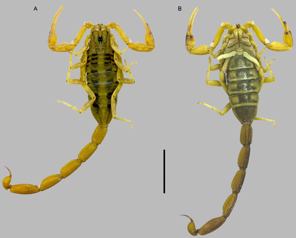
Figure 3. Habitus of female of C. balsasensis, scale = 1 cm.
Holotype specimen: was not localized in the CNAN. The only available information from the original description is as follow: “El holotipo es un macho adulto recolectado en Churumuco, municipio del mismo nombre en Michoacán, México el 08 de junio de 2000 por Erwin P. Miranda López y será depositado en la Colección Nacional de Arácnidos del Instituto de Biología de la Universidad Nacional Autónoma de México (CNA-IBUNAM)”.
Records from literature: Córdova-Athanasiadis (2005): México, Morelos, Municipality of Amacuzac: Huajuntlán, 18°36’36.00” N, 99°25’48.00” W, 1,510 m, 4-09-2004, M. Córdova, A. Gotilla, 5 ♀, CNAN-SC106. San Gabriel de las Palmas, 18°36’36.00” N, 99°21’00.00” W, 1,420 m, 4-09-2004, M. Córdova, A. Gotilla, 8 ♀, CNAN-SC131. Municipality of Axochiapan: Quebrantadero, 18°31’48.00” N, 98°47’24.00” W, 1,280 m, 2-09-2003, M. Córdova, D. Morán, 8 ♀, 6 ♂, 2 juv., CNAN-SC105. Municipality of Coatlán del Río: El Oyanco, 18°43’48.00” N, 99°25’48.00” W, 1,022 m, 6-08-2004, M. Córdova, O. Sotelo, 17 ♀, 6 ♂, CNAN-SC132. Municipality of Emiliano Zapata: Temimilcingo, 18°44’24.00” N, 99°09’00.00” W, 1,060 m, 28-04-2004, M. Córdova, A. Jaimes, 6 ♀, 4 ♂, CNAN-SC74. Municipality of Jonacatepec: Chalcatzingo, 18°40’48.00” N, 98°46’12.00” W, 1,371 m, 5-04-2004, M. Córdova, D. Morán, 11 ♀, 6 ♂, CNAN-SC978. Las Trancas, 13-11-1938, 2 ♀, CNAN-SC185. Municipality of Miacatlán: Palpan, 18°51’00.00” N, 99°25’12.00” W, 1,587 m, 7-08-2004, M. Córdova, O. Vázquez, 3 ♀, CNAN-SC93. Municipality of Temixco: Pueblo Viejo, 18°52’12.00” N, 99°15’00.00” W, 1,378 m, 11-06-2004, M. Córdova, A. Jaimes, O. Sotelo, 6 ♀, 6 ♂, 1 juv., CIBUAEM. Municipality of Tepalcingo: Cerro del Venado, 18°36’36.00” N, 98°51’36.00” W, 1,380 m, 1-09-2003, M. Córdova, D. Morán, 17 ♀, 9 ♂, CNAN-SC80. El Limón, 18°32’24.00” N, 98°55’48.00” W, 1,191 m, 12-09-2004, M. Córdova, G. Obregón, 4 ♀, 7 ♂, CIBUAEM. Municipality of Tlaltizapán: Barranca Honda, 18°49’12.00” N, 99°06’00.00” W, 1,200 m, 20-06-2004, M. Córdova, M. Barrios, 4 ♀, 2 ♂, CNAN-98; M. Córdova, M. Barrios, 1 ♀, 18 juv., CNAN. Municipality of Tlalquiltenango: Chimalacatlán, 18°27’36.00” N, 99°06’00.00” W, 1,066 m, 11-07-2004, M. Córdova, O. Sotelo, 4 ♀, 5 ♂, CNAN-SC976. Huautla, 18°23’24.00” N, 99°01’48.00” W, 976 m, 12-07-2004, M. Córdova, A. Jaimes, 17 ♀, 8 ♂, 1 juv., CNAN-SC81; 1 ♀, 24 juv., CNAN; 18°26’24.00” N, 99°01’12.00” W, 11-06-1994, A. Burgos, 3 ♀, CIBUAEM. Quilamula, 18°31’12.00” N, 99°01’12.00” W, 1,100 m, 7-06-2004, M. Córdova, E. Maison, 2 ♀, 3 juv., CIBUAEM; 15-08-2003, M. Córdova, A. Jaimes, H. Lagunas, 11 ♀, 9 ♂, 2 juv., CNAN-SC165. Xicatlacotla, 18°33’36.00” N, 99°13’48.00” W, 812 m, 26-06-2004, M. Córdova, 1 ♀, 28 juv., CNAN-SC917; 3♀, CIBUAEM. Xalostoc, 18°43’12.00” N, 98°54’00.00” W, 1,602 m, 21-11-2003, M. Córdova, 6 ♀, 1 ♂, CNAN-SC159. Municipality of Yautepec: San Isidro, 18°49’12.00” N, 99°06’00.00” W, 1,378 m, 20-06-2004, M. Córdova, M. Barrios, 5 ♀, 1 ♂, CNAN-SC96; 1 ♀, 19 juv., CNAN. Municipality of Zacatepec: Galeana, 15-08-1991, G. Peña, 4 ♀, 3 ♂, 2 juv., CIBUAEM. Zacatepec, 30-06-1981, F. Guerrero, 3 ♀, CNAN-SC118. Municipality of Zacualpan de Amilpas: El Curiel, 18°46’48.00” N, 98°45’36.00” W, 1,668 m, 31-07-2004, M. Córdova, O. Sotelo, A. Sotelo, 18 ♀, 4 ♂, 1 juv., CNAN-SC79. Ponce-Saavedra & Francke (2004): México, Guerrero, Municipality of Tzirándaro: 18°28’25” N, 100°57’17” W. Michoacán, Municipality of Apatzingán: Altamira, El Tesorero, 18°57’42” N, 102°22’58” W. Las Anonas, 18°51’36” N, 102°35’00” W. Valle Verde, 19°02’54” N, 102°23’18” W. Municipality of Arteaga: El Descansadero, 19°34’17” N, 101°49’17” W. El Puerto, road to Tumbiscatío, 18°09’18” N, 102°23’18” W. Las Cañas, 18°33’20” N, 101°58’19” W. Municipality of Buenavista Tomatlán: Buenavista, 19°120’24” N, 102°35’12” W. El Puerto, 19°14’48” N, 102°35’37” W. Municipality of Carácuaro: 19°00’54” N, 102°07’05” W. Km 4 from San Antonio de las Huertas towards Carácuaro, 19°06’13” N, 101°12’06” W. Municipality of Churumuco: Cerro de Las Letras, 18°39’37” N, 101°39’17” W. Churumuco, 18°39’48” N, 101°38’64” W. El Ahuijote, 18°42’30” N, 101°46’00” W. Potrero de Corpus, El Chocolate, 18°52’48” N, 101°37’47” W. Municipality of Gabriel Zamora: Cerro de la Cruz, 19°09’55” N, 102°04’03” W. El Jagüey, 19°10’49” N, 102°01’24” W. El Ranchito, 19°11’00” N, 102°03’11” W. Km 128 Morelia-L.C road, 19°04’51” N, 102°00’59” W. Municipality of Huacana: Presa de Zicuirán, 18°55’18” N, 101°55’49” W. Municipality of Huetamo: road to Baztán, near El Rodeo, 18°46’13” N, 100°59’54” W. Cerro de Turitzio, near Arúa, 18°31’49” N, 100°55’45” W. Municipality of Mújica: Km 135 road La Huacana-Cuatro Caminos, 18°31’49” N, 100°55’45” W. Nueva Italia, 19°01’24” N, 102°05’30” W. Municipality of Nuevo Urecho: breach towards Nueva Jerusalem, 19°05’06” N, 101°30’15” W. Km 3.8 road Puruarán-Turicato, 19°’05’48” N, 101°30’24” W. Municipality of Parácuaro: La Tuna, 19°05’48” N, 102°13’55” W. Municipality of San Lucas: 18°35’12” N, 100°47’11” W. Municipality of Tacámbaro: Arroyo Frío, 19°10’53” N, 101°28’30” W. Municipality of Taretán: 19°20’00” N, 101°55’05” W. Municipality of Tepalcatepec: El Taixtán, 19°00’49” N, 102°59’12” W. Estado de México, Municipality of Tejupilco: 1 km SE of Mango Matus, 18°40’00” N, 100°26’39” W. Quijano-Ravell & Ponce-Saavedra (2016): México, Michoacán, Municipality of Churumuco: 18°39’39.00” N, 101°38’46.00” W, 4 ♀, 3 ♂. Municipality of Huetamo: Arúa, 18°32’25.00” N, 100°55’35.00” W, 3 ♀, 4 ♂. Reyes-Moya et al. (2021): Mexico, Chihuahua, Municipality of Ciudad Juárez: 31°38’31” N,106°26’34.4” W, 03/04-2019.
Examined material: México, Aguascalientes, Municipality of Aguascalientes: Universidad Autónoma de Aguascalientes, 18-05-2012, N. Ubario-Guevara, 1 ♀, CZUAA SCO-107; 15-05-2016, A. A. Martínez-Durón, 1 ♀, CZUAA SCO-411. Jardín Botánico Rey Netzahualcóyotl, 25-04-2014, J. E. Gutiérrez-Montoya, 1 ♀, CZUAA SCO-106; 04-2015, J. E. Díaz-Plascencia, 3 ♀, CZUAA SCO-108. Fraccionamiento Casa Blanca, 13-04-2016, M. A. Delgado, 1 ♀, CZUAA SCO-434. Fraccionamiento El Dorado, 14-10-2019, 1 ♀, CZUAA SCO-551. Tlaxcala #107, colonia San Marcos, 21-06-2020, V. Esparza, 4 ♀, CZUAA SCO-535. Pozo Hondo 141, colonia Pozo Bravo, 29-06-2020, N. Palacios, 1 ♀, CZUAA SCO-546. Tlaloc 519, colonia Prados del Sur, 8-03-2022, I. Martínez, 1 ♀, CZUAA SCO-672. Municipality of Calvillo: Colomos, plantación de guayaba, 21°52’44.11” N, 102°39’16.70” W, 1,798 m, 27-01-2022, I. J. Rodríguez-Elizalde, J. Brito-Ruiz de Velasco, 1 ♀, CZUAA SCO-686; 29-08-2021, I. J. Rodríguez-Elizalde, J. Brito-Ruiz de Velasco, L. I. Rodríguez-Rodríguez, M. E. Herrera-Rodríguez, 1 ♀, CZUAA SCO-692. El Terrero, 17-04-2011, J. Ruvalcaba-Calderón, 1 ♀, CZUAA SCO-104. Los Adobes, 21°48’39.22” N, 102°41’21.34” W, 1,875 m, 17-09-2019, F. Chávez-Samayoa, L. R. Haro-Tapia, 4 ♀, CZUAA SCO-509; 21°48’39.22” N, 102°41’57.34” W, 1,875 m, 11-10-2019, F. Chávez-Samayoa, 2 ♀, CZUAA SCO-698. Calvillo, 10-11-2021, R. García, 2 ♀, CZUAA SCO-670. Municipality of Jesús María: Alegría #122, colonia Gómez Portugal, 23-03-2022, 1 ♀, CZUAA SCO-695. Cerro del Muerto, 8-05-2005, A. Ramírez, 1 ♀, CZUAA SCO-111. Michoacán, Municipality of Uruapan: F. A. Guerrero-Roque, 1 ♀, CZUAA SCO-54. Zacatecas, Municipality of Jalpa: 21-04-2016, V. E., 1 ♀, CZUAA SCO-407. Municipality of Juchipila: 25-04-2010, C. Y. Gómez-Aranzazú, 2 ♀, CZUAA SCO-102; 13-05-2000, D. Magaña-Ortíz, 1 ♀, CZUAA SCO-110.
Remarks
Other than the Churumuco site (18°39’48” N, 101°38’64” W), in the Michoacan Balsas Depression, C. balsasensis has been recorded in the states of Guerrero, Mexico, Morelos, and Puebla (Córdova-Athanasiadis, 2005; Ponce-Saavedra & Francke, 2004; Ponce-Saavedra et al., 2022; Santibáñez-López et al., 2015). However, the records from Morelos are questionable (González-Santillán & Possani, 2018).
Reyes-Moya et al. (2021) recently recorded C. balsasensis in Ciudad Juárez, Chihuahua, indicating that the species collected may represent an “accidental introduction” into the city likely due to (Ciudad Juárez is) “the northern largest and busiest border crossing of Mexico and the USA, experiencing massive local and non-local human transit”. We were able to examine some of the specimens cited in that contribution and concluded that they are not conspecific with C. balsasensis. We base our conclusion on the comparison of the following set of the characters readily observed in their published figures: 1) there is an areola created by pigmentation circling each median ocellus on the carapace in Reyes-Moya et al. (2021, their Fig. 1A), whereas in the original description of Ponce-Saavedra & Francke, 2004 (their Fig. 9), in Quijano-Ravell & Ponce-Saavedra 2016 (their Fig. 6[2]), and in our figure 4A, the areola is not complete with the retrolateral area lacking pigmentation; 2) the body length of the females in Reyes-Moya et al. (2021) is 37 and 40 mm, whereas in the original description, the body length is 60 and 73 mm, a difference of more than 20 mm; 3) the pectens’ basal piece of the females is wider than longer (Reyes-Moya et al., 2021), but those of the original description are trapezoid, almost as long as wide, with a deep medial depression. The description of the specimens provided by Reyes-Moya et al. (2021), however, is more like Centruroides sculpturatus, particularly due to the pigmentation pattern of the carapace and tergites exhibited by phase 2 or 3 identified by Stahnke (1971). The likelihood of introduction from the Balsas Basin to Ciudad Juárez is considerably lower compared to the introduction of this species from Sonora or even Arizona because of the proximity of these areas. Our conclusion is that the specimens reported and illustrated by Reyes-Moya et al. (2021) are conspecific to C. sculpturatus instead of C. balsasensis.

Figure 4. Carapace of C. balsasensis (A) and C. infamatus (B).
We recorded C. balsasensis for the first time in Aguascalientes with 20 samples (32 individuals) from the Municipalities of Aguascalientes, Calvillo, and Jesús María. The first sample dates to 2005 (CZUAA SCO 111), and the most recent one to May 2023 (CZUAA SCO-732). Specimens deposited in the CZUAA were associated mainly with urban areas or meadows. Remarkably, we only observed adult or juvenile females; males are absent in the collection. It is likely that this species was transported accidentally and has invaded Aguascalientes and other northern states (we also examined 3 samples from Zacatecas: CZUAA SCO-102, CZUAA SCO-110, CZUAA SCO-407). However, further investigation to elucidate the establishment of this species is needed. Our data also suggest that the establishment of the population in Aguascalientes may have occurred by parthenogenesis due to the presence of only females in colonized urban and suburban areas. This hypothesis finds support by the occurrence of the same phenomenon in the South American species Tityus serrulatus, Lutz and Mello, 1922, which exhibits indigenous sexual populations and asexual populations in colonized habitats (Braga-Pereira & Santos, 2021). Intriguingly, this is also a medically relevant species in Brazil, suggesting parallel ecological mechanisms to establish in novel locations in different parts of the world.
Centruroides infamatus (C. L. Koch, 1844) (Fig. 5)
Taxonomic summary
Holotype specimen: Zoologisches Museum, Humbolt Universität, Berlin, Germany. Sex and type locality unknown (Fet & Lowe, 2000).
Records from literature: Esposito et al. (2018): México, Michoacán, Municipality of Tangamandapio: Los Tabanos, 19°58’29.64” N, 102°50’32.14” W, 223 m, 31-05-2006, O. F. Francke, H. Montaño, A. Valdez, A. Ballesteros, 2 ♀, AMCC (LP6420). Municipality of Tingambato: Tingambato 4 km W, under stones, 23-03-2000, E. González, 1 ♂, AMCC (LP1822). Ponce-Saavedra & Francke (2004): México, Guanajuato, Municipality of Romita: San Antonio del Pochote, 20°55’47.00” N, 101°33’48.00” W. Michoacán, Municipality of Coalcomán: 18°48’47.00” N, 103°09’57.00” W. Municipality of Morelia: 19°42’00.00” N, 101°11’18.00” W. Tiripetío, 19°32’00.00” N, 101°21’00.00” W. Municipality of Salvador Escalante: Salvador Escalante, 19°24’00.00” N, 101°38’18.00” W. Municipality of Uruapan: La Cofradía, 19°26’00.00” N, 102°01’00.00” W. Zumpimito, 19°22’18.00” N, 102°03’19.00” W. Ponce-Saavedra et al. (2009): México, Michoacán, Municipality of Uruapan: Zumipito, 19°21’25.00” N, 102°04’13,00” W, GenBank AF439753. Quijano-Ravell & Ponce-Saavedra (2016): México, Guanajuato, Municipality of León: 21°01’02.00” N, 101°37’44.00” W, 3 ♂ 2 ♀. Michoacán, Muncipality of Uruapan: Zumipito, 21°07’30.00” N, 101°01’49.00” W, 4 ♂ 4 ♀.

Figure 5. Habitus of male (top) and female (bottom) of C. infamatus, scale = 1 cm.
Examined material: Mexico, Aguascalientes, Municipality of Aguascalientes: Central de abastos, 02-1996, J. G. Estrada-A., 1 ♂, CZUAA SCO-54. Cerro de los Gallos, 21-10-1989, L. Silva-López, 1 ♀, CZUAA SCO-117; 26-04-1984, H. Gallegos-Rangel, 1 ♀, CZUAA SCO-118. Municipality of Calvillo: Cascada Los Huenchos, 21°52’52.90” N, 102°47’06.25” W, 1756 m, 22-05-2021, J. L. Reyes-Hernández, 1 ♂, CZUAA SCO-614. Cercano a balneario “La Cueva”, 21°48’47.70” N, 102°49’34.82” W, 28-09-2019, F. Chávez-Samayoa, L. R. Haro-Tapia, 1 ♀, CZUAA SCO-483; 15-10-2019, F. Chávez-Samayoa, 19 ♂, 10 ♀, CZUAA SCO-495; 19-10-2019, F. Chávez-Samayoa, 23 ♂, 12 ♀, CZUAA SCO-503. Cercano a restaurante “La Fragua”, 21°59’52.32” N, 102°40’35.36” W, 1,825 m, -05-2021, T. Huerta, 3 ♂, 2 ♀, CZUAA SCO-644. El Cuervero, 19-06-2004, A. D. González, 1 ♀, CZUAA SCO-162. El Zapote, 8-12-2021, R. García, 1 ♀, CZUAA SCO-666. Calvillo, 29-04-2017, E. M. Flores-Villalpando, 1 ♀, CZUAA SCO-431; 4-05-2017, A. Hernández, 1 ♀, CZUAA SCO-435. Crucero de las Pilas, 11-11-2020, R. García, 1 ♂, CZUAA SCO-700. La Calixtina, 16-05-2017, I. Rodríguez-Ortiz, 1 ♀, CZUAA SCO-424. La Labor, 10-04-2011, M. P. Ramírez-Guillen, 1 ♂, CZUAA SCO-139. La Mezquitera, 21°51’37.47” N, 102°46’04.20” W, 30-08-2019, F. Chávez-Samayoa, J. A. Escoto-Moreno, 1 ♂, 1 ♀, CZUAA SCO-484; 5-10-2019, F. Chávez-Samayoa, 23 ♂, 8 ♀, CZUAA SCO-508; 7-09-2019, F. Chávez-Samayoa, R. Haro-Tapia, 4 ♂, 2 ♀, CZUAA SCO-514; 10-10-2019, F. Chávez-Samayoa, 2 ♂, CZUAA SCO-558. Los Adobes, 21°48’39.22” N, 102°41’21.34” W, 1-09-2015, J. E. Díaz-Plascencia, 1 ♀, CZUAA SCO-330; 11-10-2019, F. Chávez-Samayoa, 15 ♂, 4 ♀, CZUAA SCO-480; 17-09-2019, F. Chávez-Samayoa, R. Haro, 26 ♂, 13 ♀, CZUAA SCO-497; 6-09-2019, J. A. Escoto-Moreno, F. Chávez-Samayoa, 1 ♂, CZUAA SCO-555. Los Alisos, 9-10-1989, J. Moreno-Lara, 1 ♂, CZUAA SCO-121; 2-06-1982, Z. M. Vela-Ortiz, 1 ♂, CZUAA SCO-133; 8-09-1984, Morales, Franco, Montoya, 1 ♂, CZUAA SCO-134; 19-06-2004, G. Guerrero, 1 ♀, CZUAA SCO-154. Los Lobos, 21-10-1990, J. A. Sánchez-García, 1 ♀, CZUAA SCO-129. Presa Malpaso, 19-06-2004, G. Villalobos, 1 ♂, CZUAA SCO-123; 3-05-1999, R. P. Arteaga-Hernández, 1 ♂, CZUAA SCO-125; 13-06-2004, E. Ortiz-Martínez, 1 ♂, CZUAA SCO-126; 20-03-1999, M. Morga, 1 ♂, CZUAA SCO-131; 3-05-1999, M. Martínez-Garnica, 1 ♀, CZUAA SCO-135; 26-11-1986, E. Alvizo-Flores, 1 ♀, CZUAA SCO-138. Palo Alto, 18-11-2021, R. García, 1 ♂, 3 ♀, CZUAA SCO-671; 20-11-2021, R. García, 4 ♂, CZUAA SCO-667. Presa La Codorniz, 22°00’39.07” N, 102°40’15.19” W, 1,894 m, 1-11-2020, E. González-Martínez, J. L. Reyes-Hernández, I. E. Gallegos-Vieyra, D. F. Simijaca-Salcedo, F. Chávez-Samayoa, 5 ♂, 5 ♀, CZUAA SCO-589; 21°59’50.78” N, 102°40’42.78” W, 2,068 m, 5-06-2021, F. Chávez-Samayoa, D. Ortiz-Álvarez, C. Huerta, 5 ♂, 10 ♀, CZUAA SCO-612. Presa La Ordeña, 25-04-2005, C. A. Díaz-Delgado, 1 ♀, CZUAA SCO-145. Presa de los Serna, 20-10-2003, S. García, 1 ♀ CZUAA SCO-124; 14-06-2004, S. García, 1 ♀, CZUAA SCO-137. San Tadeo, -04-1996, J. Martínez-de Lara, 1 ♀, CZUAA SCO-127; -05-2015, C. A. Franco-Servín de la Mora, 1 ♂, 2 ♀, CZUAA SCO-149. Sierra del Laurel, 25-10-1982, E. Padilla-R., 1 ♂, CZUAA SCO-128. Terrero de la Labor, 22°01’32.02” N, 102°39’58.00” W, 22-10-2021, F. Chávez-Samayoa, D. Ortiz-Álvarez, 25 ♂, 20 ♀, CZUAA SCO-655. Municipality of Jesús María: Cerro El picacho, 23-05-2014, E. A. Hernández-Medrano, 1 ♂, CZUAA SCO-109; 29-04-2016, D. Martínez, 1 ♂, CZUAA SCO-418. Municipality of Rincón de Romos: 17-04-2004, N. Arroyo-Chávez, 1 ♂, CZUAA SCO-112; 17-04-2004, A. F. Ramos-Martínez, 1 ♂, CZUAA SCO-113. Guanajuato, Municipality of Comonfort: 04-2007, D. García, 1 ♂, CZUAA SCO-402. Municipality of León: Fraccionamiento La Luz, 27-04-2013, V. H. González-Sánchez, 1 ♀, CZUAA SCO-75; 27-04-2003, K. A. de Luna-Gómez, 1 ♀, CZUAA SCO-85. León, 30-05-2009, C. García-Balderas, 1 ♀, CZUAA SCO-77; 13-06-2004, C. Moreno, 1 ♂, CZUAA SCO-84; 21-06-2004, M. A. Gómez, 1 ♂, CZUAA SCO-87; 4-06-2000, M. Chávez-Andrade, 1 ♂, CZUAA SCO-88; 7-06-2004, S. Flores, 1 ♂, CZUAA SCO-90; 15-06-2004, M. A. B. López, 1 ♂, CZUAA SCO-94; 16-06-2006, Miguel, 1 ♀, CZUAA SCO-96; R. A. Carbajal-Márquez, 1 ♀, CZUAA SCO-99. Municipality of Moroleón: Presa Quiahuyo, 25-03-2016, K. Rosales, 1 ♀, CZUAA SCO-445. Municipality of Pénjamo: 21-09-1983, O. A. Rodríguez, M. G. Flores, 1 ♀, CZUAA SCO-79. Municipality of Salamanca: L. Flores, 1 ♂, CZUAA SCO-70; J. A. Berlín-Diosdado, 1 ♀, CZUAA SCO-71. Municipality of Yuriria: 13-06-1991, V. Villalobos-Sánchez, 1 ♀, CZUAA SCO-74. Michoacán, Municipality of Uruapan: M. A. Domínguez-de la Riva, 1 ♀, CZUAA SCO-51. Municipality of Tancítaro: El Cuate, -04-1996, R. E. Martínez, 1 ♀, CZUAA SCO-58. Zacatecas, Municipality of Guadalupe Victoria: 9-11-1986, M. Torres-Romero, 1 ♂, CZUAA SCO-60. Municipality of Juchipila: 16-04-2016, K. I. Molina, 1 ♂, CZUAA SCO-413; 25-03-2016, E. A. Bernal-Montoya, 1 ♀, CZUAA SCO-425; 15-05-2016, A. Barba, 1 ♂, CZUAA SCO-448. Municipality of Nochistlán: 2-03-2010, E. F. Pulido-Hornedo, 1 ♀, CZUAA SCO-53. Municipality of Tabasco: 10-06-2010, A. Lara, 1 ♂, CZUAA SCO-57. Municipality of Valparaiso: 4-04-2017, S. D. López-González, 1 ♂ CZUAA SCO-416.
Remarks
Known records for C. infamatus include the southern half of Aguascalientes, northwestern Guanajuato, Jalisco, Michoacán, and the southern third of Zacatecas (González-Santillán & Possani, 2018). State records without precise locality information were published for Colima, Durango, Nayarit, Oaxaca, Puebla, Querétaro, and Sinaloa (Ponce-Saavedra & Francke, 2013a; Ponce-Saavedra et al., 2022; Santibáñez-López et al., 2015).
Centruroides infamatus is a component of Aguascalientes species richness, and before our work, it was the only species of medical importance reported for the state. This species inhabits the area corresponding to the Trans Mexican Volcanic Belt biogeographic province. However, its distribution in Aguascalientes is restricted to the southwestern municipalities, most abundantly in Calvillo, which corresponds to the lower lands of the Pacific biogeographic province. Centruroides infamatus was recorded in high densities in altitudes between 1,700 and 2,100 m on the slopes of a canyon formed by the Sierra del Laurel and Sierra Fría. We hypothesized that as part of the diversification of the infamatus species group of the genus Centruroides (sensu Ponce-Saavedra & Francke, 2019), the populations established in this area of Aguascalientes and most likely in Zacatecas, may represent a separate species from the Trans Mexican Volcanic Belt biogeographic province populations due to their geographical disjunction created by the Sierra del Laurel to the east and the arid zone corresponding to the Chihuahuan desert, north to the Aguascalientes City. In another scenario, we surmise that this species may be a component of the Pacific Lowlands province that has penetrated the mainland and most likely represents a distinctively independent taxon from the populations inhabiting the Trans Mexican Volcanic Belt. Further molecular and ecological studies may clarify these hypotheses.
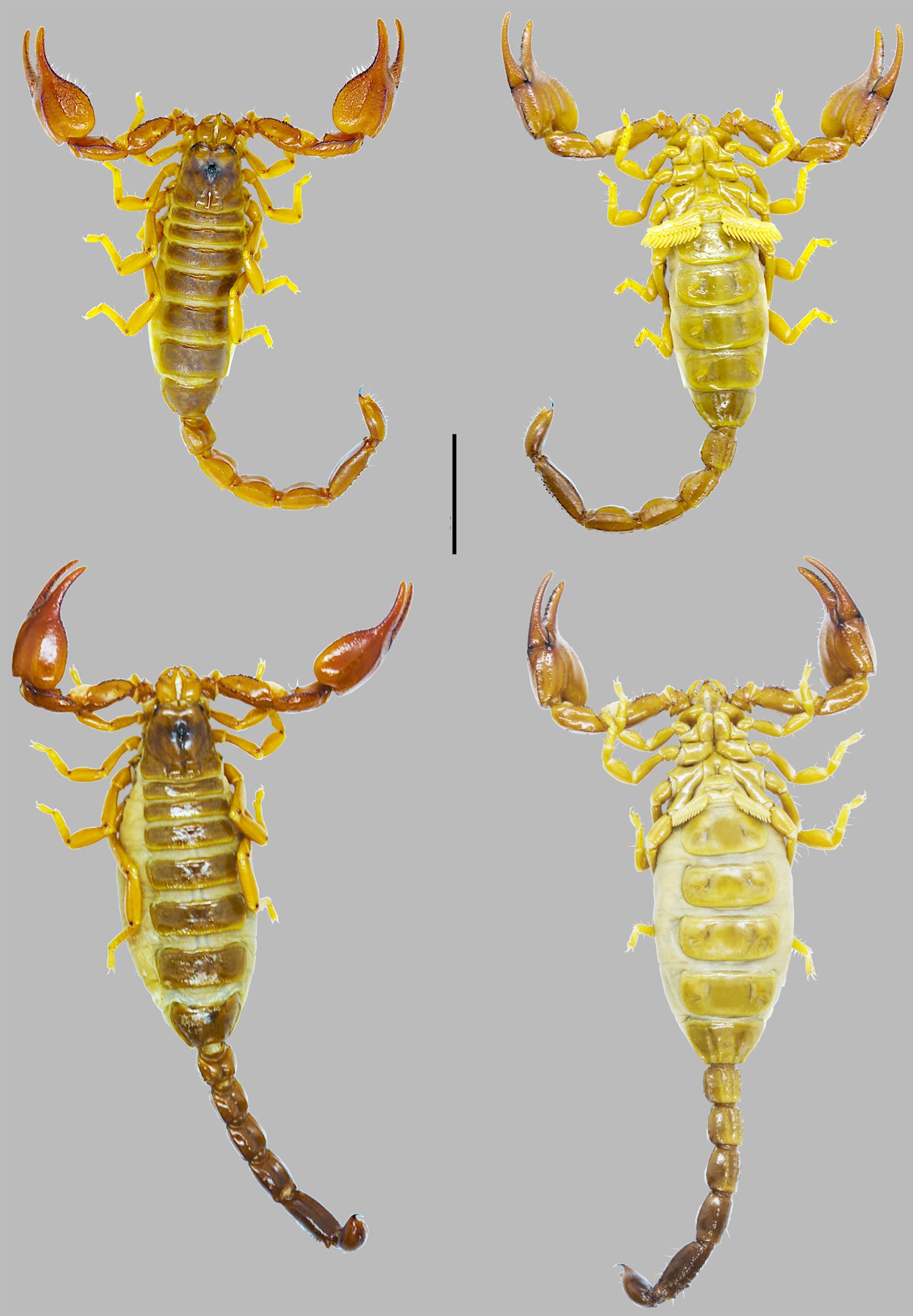
Figure 6. Habitus of male (top) and female (bottom) of D. zacatecanus, scale = 1 cm.
Diplocentridae Karsch, 1880
Diplocentrus zacatecanus Hoffmann, 1931 (Fig. 6)
Taxonomic summary
Lectotype: deposited in the CNAN. México: Aguascalientes: Tepezalá (22°13.3629’ N, 102°10.0149’ W, 2,100 m.), no date or collector 1 ♂ (CNAN-T0761). Paralectotypes: 2 ♂♂ and 1 ♀ (CNAN-T0762) same locality and collection event (Santibáñez-López & Francke, 2013).
Records from literature: Hoffmann (1931): México, Aguascalientes, Municipality of Tepezalá. Zacatecas, Municipality of Pinos. Ponce-Saavedra et al. (2009): México, Aguascalientes, Municipality of Tepezalá: 22°13’20.94” N, 102°10’17.53” W, 2100 m. Durango, Municipality of San Juan de Guadalupe: Loma Alta, 24°37’58.05” N, 102°45’2.80” W, 1,560 m. Vicente Guerrero, 23°43’53.99” N, 103°59’14.55” W, 1,922 m. Estado de México, Municipality of Aculco: La Loma, 20°06’07.03” N, 99°51’25.71” W, 2,450 m. Municipality of Soyaniquilpan: San José Deguedo, 20°05’09.04” N, 99°33’48.78” W, 2,514 m. Guanajuato, Municipality of Coroneo, 20°11’54.81” N, 100°21056.60” W, 2,280 m. Hidalgo, Municipality of Tula de Allende: Michimaloya, 20°05’34.88” N, 99°23’57.93” W, 2,078 m. Michoacán, Municipality of Contepec: 19°57’10.44” N, 100°09’48.90” W, 2,480 m. Querétaro, Municipality of Cadereyta: Cadereyta, 20°41’38.29” N, 99°48’36.21” W, 2037 m. El Organal, 20°37’09.49” N, 99°38’27.98” W, 1,733 m. Vizarrón de Montes, 20°50’03.63” N, 99°43’09.27” W. Municipality of Huimilpan: 20°22’22.23” N, 100°16’27.48” W, 2,288 m. San Luis Potosí, Municipality of Villa de Ramos: 22°49’53.21” N, 101°54’36.01” W, 2,200 m. Zacatecas, Municipality of Cañitas de Felipe Pescador: 23°36’20.10” N, 102°43’47.50” W, 2,027 m. Municipality of Sain Alto: Emiliano Zapata, 23°34’16.66” N, 103°18’02.75” W, 2,067 m. Municipality of Zacatecas: 22°46’19.52” N, 102°34’32.01” W, 2,440 m. Santibáñez-López and Francke (2013): México, Aguascalientes, Municipality of Tepezalá: 22°13’21.77” N, 102°10’00.89” W, 2,100 m, CNAN-T0761, lectotype, 1 ♂; CNAN-T0762, paralectotypes, 2 ♂, 1 ♀; 1 km N, 22°14’20.88” N, 102°10’28.02” W, 2,048 m, 4 ♂, CNAN-S03075, 4-07-2005, O. F. Francke, J. Ponce-Saavedra, M. Córdova, A. Jaimes, G. Francke, V. Capovilla, 2 ♂, AMNH. Zacatecas, Road Sombrerete-Durango: km 179, 23°40’47.88” N, 103°41’42.72” W, 2,448 m, 9-08-2005, O. F. Francke, W. D. Sissom, C. Lee, K. McWest, L. Jarvis, C. Durán, H. Montaño, A. Ballesteros, 3 ♀, CNAN-SC1731; 3 ♀, AMNH.
Examined material: Mexico, Aguascalientes, Municipality of Asientos: Asientos, 10-02-2013, V. Martínez-Salazar, 1 ♀, CZUAA SCO-06; 17-03-2013, C. Franco-Servín de la Mora, 1 ♀, CZUAA SCO-10; 22-02-2013, R. A. Rosales, 1 ♀, CZUAA SCO-12. Municipality of El Llano: Juan el Grande, 21°56’21.00” N, 101°55’06.00” W, 2,495 m, 18-10-2019, N. A. Pulido-Hornedo, X. A. Ruiz, 3 ♀, CZUAA SCO-473; 18-10-2019, F. Chávez-Samayoa, 4 ♂, 6 ♀, CZUAA SCO-475; 21°55’54.55” N, 101°56’09.28” W, 2,117 m, 22-09-2019, F. Chávez-Samayoa, 2 ♂, 4 ♀, CZUAA SCO-490; 21°56’14.57” N, 101°55’24.35” W, 2,285 m, 1-06-2020, P. C. Hernández-Romero, D. F. Simijaca-Salcedo, F. Chávez-Samayoa, 1 ♀, CZUAA SCO-541; 21°56’21.08” N, 101°55’17.87” W, 2,395 m, -10-2019, E. González-Martínez, 1 ♂, 2 ♀, CZUAA SCO-543; 22-01-2021, F. Chávez-Samayoa, A. Palacios, D. F. Simijaca-Salcedo, 1 ♂, CZUAA SCO-633; 21°56’14.57” N, 101°55’24.35” W, 2,284 m, -04-2021, F. Chávez-Samayoa, D. F. Simijaca-Salcedo, 1 ♂, CZUAA SCO-645; -03-2021, F. Chávez-Samayoa, D. M. Reyes-Páramo, 1 ♀, CZUAA SCO-652. Municipality of Tepezalá: Cerro del Capulín, 22°14’45.06” N, 102°09’14.90” W, 2,189 m, 6-10-2019, F. Chávez-Samayoa, I. Villalobos-Juárez, E. González-Martínez, 2 ♂, 2 ♀, CZUAA SCO-488; 13-10-2019, F. Chávez-Samayoa, 5 ♀, CZUAA SCO-505; 22°14’01.00” N, 102°09’27.58” W, 2,130 m, 21-08- 2020, F. Chávez-Samayoa, 2 ♀, CZUAA SCO-525; 30-11-2020, I. Villalobos-Juárez, D. F. Simijaca-Salcedo, F. Chávez-Samayoa, 1 ♀, CZUAA SCO-595; 25-04-2021, F. Chávez-Samayoa, D. F. Simijaca-Salcedo, I. Villalobos-Juárez, 1 ♂, CZUAA SCO-662. Tepezalá, -04-2006, O. Ortega, 1 ♂, CZUAA SCO-01; -03-2006, M. de la Riva, 1 ♂, CZUAA SCO-02; 27-04-2006, L. Reséndiz, 1 ♂, CZUAA SCO-04; -04-2006, R. A. Carbajal, 1 ♀, CZUAA SCO-07; -06-2006, L. Flores, 1 ♀, CZUAA SCO-09; -06-2006, J. Salazar-López, 1 ♀, CZUAA SCO-11; 15-06-2006, E. Medina-Alcantar, 1 ♂, CZUAA SCO-15; 15-06-2006, V. Revilla-Castellanos, 1 ♀, CZUAA SCO-16; 28-02-2006, M. Domínguez-De la Riva, 1 ♀, CZUAA SCO-17; -03-2006, D. Rendón, 1 ♀, CZUAA SCO-18; -05-2006, F. A. Guerras-Roque, 1 ♀, CZUAA SCO-20. San Luis Potosí, Muncipality of San Luis Potosí: Cerro de San Pedro, 7-04-2007, L. Argüello, 1 ♀, CZUAA SCO-449.
Remarks
This species is recorded from Aguascalientes, Durango, Estado de México, Guanajuato, Hidalgo, Michoacán, Querétaro, San Luis Potosí, and Zacatecas (Ponce-Saavedra et al., 2009; Santibáñez-López & Francke, 2013).
Formerly a subspecies of Diplocentrus keyserlingii Karsch, 1880, it was described by Hoffmann from specimens collected in the Municipality of Tepezalá, Aguascalientes. We confirmed its presence in the type locality Tepezalá and additionally in the Municipalities of El Llano and Asientos. Diplocentrus zacatecanus inhabits the portion of the state that belongs to the Chihuahuan Desert biogeographic province (Morrone et al., 2017), which is nearly half of Aguascalientes’s surface.
The external morphology and the hemispermatophore of D. zacatecanus are either conserved or too variable to delimit species (Santibáñez-López & Francke, 2013). One possible explanation is the propensity of being substrate specialists and their strong adaptation to construct galleries where they spend most of their life exhibiting scarcely superficial activity. Diplocentrus zacatecanus is a substrate specialist requiring a particular type of soil, like other pelophilous species (Polis, 1990; Prendini, 2001). Soil-type discontinuity hinders its dispersal, promoting isolated populations and may promote allopatric speciation. Due to its wide distribution range in Mexico, D. zacatecanus may comprise a species complex that needs molecular studies to clarify and guide the correct species delimitation within such a broad distribution area.
Vaejovidae Thorell, 1876
Syntropinae Kraepelin, 1905
Chihuahuanus bilineatus (Pocock, 1989) (Fig. 7)
Taxonomic summary
Holotype: British Museum of Natural History, London, UK: San Diego Texas, USA. 1 ♀. Williams (1970) and Sissom (2000) indicated that this is a spurious locality and is not found in Texas.

Figure 7. Habitus of male (top) and female (bottom) of C. bilineatus, scale = 1 cm.
Records from literature: Hoffmann (1931): México, Aguascalientes, Municipality of Tepezalá: 20 exemplars (♂, ♀). González-Santillán and Prendini (2013): México, Tamaulipas, Municipality of Jaumave: El Salto, between Palmillas and Jaumave, 23°21’26.39” N, 99°30’56.45” W, 1,115 m, 23-08- 2006, O. F. Francke, W.D. Sissom, G. Casper, T. Anton, V. Torti, H. Montaño, C. Santibáñez, 1 ♂, 1 ♀, CAS(ARA-1883). González-Santillán and Prendini (2015): México, Guanajuato, Municipality of San Luis de la Paz: San Luis de La Paz, 7 km E, 21°18’42.84” N, 100°25’36.06” W, 2,117 m, 24-08-2006, O. F. Francke, W. D. Sissom, G. Casper, T. Anton, V. Torti, H. Montaño, C. Santibáñez, A. Ballesteros, 1 ♀, AMCC (LP 6594). San Luis Potosí, Municipality of Ciudad del Maíz: Puerto Santa Catarina, 22°18’13.38” N, 99°37’16.08” W, 1,214 m, 22-08-2006, O. F. Francke, W. D. Sissom, G. Casper, T. Anton, V. Torti, H. Montaño, C. Santibáñez, A. Ballesteros, 1 ♀, AMCC (LP 6507). Tamaulipas, Municipality of Jaumave: El Salto, between Palmillas and Jaumave, 23°21’26.39” N, 99°30’56.45” W, 1,115 m, 23-08-2006, O.F. Francke, W. D. Sissom, G. Casper, T. Anton, V. Torti, H. Montaño, C. Santibáñez, 1 ♂, 1 ♀, AMNH (ARA 1129). Zacatecas, Municipality of Fresnillo: Colonia Guanajuato, 23°04’44.94” N, 103°05’08.34” W, 2,250 m, 6-07-2005, O. F. Francke, J. Ponce, M. Córdova, A. Jaimes, G. Francke, V. Capovilla, 1 ♀, AMCC (LP 5306). Yahia & Sissom (1996): México, Aguascalientes, Municipality of Asientos: 3.2 km W Asientos, 2,225 m, 9-06-1956, B. Banta, 2 ♂, 1 ♀, 19 juv., AMNH. Muncipality of Tepezalá: Tepezalá, C. C. Hoffmann, 4 ♂, 4 ♀, AMNH. Coahuila, Municipality of Saltillo: 8.6 km W Buñuelos in Valle de Guerra, 15-07-1977, E. A. Liner, Chaney, 2 ♀, FSCA. Nuevo León, Municipality of La Asención: 7.24 km N La Ascension, 19-07-1975, E. A. Liner, 2 ♀, 9 juv., FSCA. 4.34 km N, 3.86 km SE La Ascension on La Caballada Road, 19-07-1975, E. A. Liner et al., 2 ♂, 3 ♀, FSCA. 12.39 km N La Ascension, 19-07-1975, E. A. Liner et al, 2 ♂, 1 ♀, FSCA. 11.1 km W El Carmen, 15-06-1976, E. A. Liner et al., 1 ♀, FSCA. 3 km S San Roberto, under cactus, 13-08-1972, N.V. Horner, 1 ♀, WDS. San Luis Potosí: 35.40 km S Huizache, 20-09-1979, J.C., J. E. Cokendolpher, 1 ♂, WDS. km 20 on highway 70, 1 juv, -03-1972, 2 ♀, 1 ♀, AMNH. Hwy 70, 112.65 km W Valles, 19-02-1970, J. A. L. Cooke, R. W. Mitchell, 1 ♂, 2 ♀, 1 juv., AMNH. Municipality of Ciudad de Maíz: near Ciudad del Maíz, 19-08-1947, C. & M. Goodnight, 1 ♀, AMNH; km 50 on Hwy 57, 18-03-1972, J. M. Rowland, TMM 1 ♂. Tamaulipas: Km 14 on Hwy 101, 22-02-1973, W. Graham, T. R. Mollhagen, C. McConnell, 3 ♂, 8 ♀, 2 juv., AMNH. Km 53 on Hwy 101, 23-02-1973, T. R. Mollhagen, 1 ♂ subadult 1 ♀, AMNH. Km 92 on Hwy 101, 22-02-1973, T. R. Mollhagen, 1 ♂, 8 ♀, AMNH. Km 15 on Hwy 19, 18-03-1972, J. A. L. Cooke, 1 ♀, AMNH. Municipality of Ciudad Victoria: Ciudad Victoria, -06-1977, F. D. White, 1 ♀, WDS. 1 km NW La Presita, 20-09-1979, J. C. & J. E. Cokendolpher, 2 ♀, WDS. Palmillas, T. Raines, 2 ♀, AMNH. Municipality of Jaumave: 6.43 km N Jaumave, 20-09-1979, J.C. & J. E. Cokendolpher, 1 ♀, WDS.
Examined material: Mexico, Aguascalientes, Municipality of Asientos: Cerro Altamira, 2015, J. E. Díaz-Plascencia 1 ♀, CZUAA SCO-470. Asientos, 21-06-2015, J. E. Díaz-Plascencia, J. L. Aguilar-Aguilar, 1 ♀, CZUAA SCO-325. Municipality of El Llano: Juan el Grande, 21°56’21.00” N, 101°55’05.99” W, 2,493 m, 18-10-2019, N. A. Pulido-Hornedo, X. A. Ruiz, 5 ♂, 20 ♀, CZUAA SCO-474; 21°56’21.00” N, 101°55’06.00” W, 2,148 m, 8-08-2020, F. Chávez-Samayoa, 1 ♂, CZUAA SCO-524; 21°56’20.00” N, 101° 55’08.90” W, 2,492 m, 20-05-2020, F. Chávez-Samayoa, D. F. Simijaca-Salcedo, 1 ♂, CZUAA SCO-540; 21°56’01.53” N, 101°55’42.29” W, 2,155 m, 25-09-2020, D. F. Simijaca-Salcedo, F. Chávez-Samayoa, 4 ♀, CZUAA SCO-577; 21°56’08.88” N, 101°55’30.72” W, 2,228 m, 22-01-2021, D. F. Simijaca-Salcedo, A. Palacios, F. Chávez-Samayoa, 2 ♀, CZUAA SCO-628; 21°56’21.88” N, 101°55’18.44” W, 2,384 m, -03-2021, F. Chávez-Samayoa, D. M. Reyes-Páramo, 2 ♂, 1 ♀, CZUAA SCO-648. Municipality of Tepezalá: Cerro del Capulín, 22°14’45.06” N, 102° 09’14.90” W, 2,189 m, 13-10-2019, F. Chávez-Samayoa, I. Villalobos-Juárez, 15 ♂, 16 ♀, CZUAA SCO-494; 22°14’19.46” N, 102° 09’58.03” W, 2,082 m, 31-05-2020, F. Chávez-Samayoa, D. F. Simijaca-Salcedo, I. Villalobos-Juárez, 1 ♂, CZUAA SCO-520; 22°14’01.00” N, 102°09’27.58” W, 2,129 m, 21-08-2020, F. Chávez-Samayoa, 4 ♀, CZUAA SCO-527; 22°13’52.88” N, 102°09’36.76” W, 2,125 m, 23-10-2020, F. Chávez-Samayoa, I. Villalobos-Juárez, I. E. Gallegos-Vieyra, D. F. Simijaca-Salcedo, 1 ♀, CZUAA SCO-575. Cerro de San Juan, ladera N, 8-10-1988, J. A. Rodríguez-Ávalos, 3 ♀, CZUAA SCO-305. Tepezalá, 22°13’54.26” N, 102°10’03.06” W, 2,116 m, 7-08-2015, M. Rodríguez, CNAN; Tepezalá, 15-06-2006, V. Revillo-Castellanos, 1 ♀, CZUAA SCO-301; 28-03-2006, Z. Y. González-Saucedo, 1 ♀, CZUAA SCO-302. Nuevo León, Municipality of Galeana: 2 km hacia mina “La Huiche”, 24°41’33.72” N, 100°03’19.91” W, 1,945 m, 28-09-2013, O. F. Francke, A. Valdez, D. Barrales, J. Cruz, A. Guzmán, CNAN-SC003911. Zacatecas, Municipality of Luis Moya: Griegos community, 15-11-1996, J. R. Treviño, 1 ♀, CZUAA SCO-303.
Remarks
Chihuahuanus bilineatus is distributed in Aguascalientes, Coahuila, Guanajuato, Nuevo León, San Luis Potosí, and Tamaulipas (Sissom, 2000; Yahia & Sissom, 1996).This species was reported for the first time in Aguascalientes by Hoffmann (1931) for the Municipality of Tepezalá. This species has an affinity for arid environments and could be classified as a lapidicolous species (González-Santillán & Prendini, 2013). It also inhabits mainly the Chihuahuan Desert province, and collection records in the state include the municipalities of Aguascalientes, Asientos, El Llano, Jesús Maria, and Tepezalá.
Chihuahuanus coahuilae (Williams, 1968) (Fig. 8)
Taxonomic summary
Holotype: California Academy of Sciences: Mexico: Coahuila: 0.5 km SW Cuatro Ciénegas de Carranza, 1 ♂ and 19 ♂♂, 25 ♀♀ paratypes (type No. 10170).

Figure 8. Habitus of male (top) and female (bottom) of C. coahuilae, scale = 1 cm.
Records from literature: González-Santillán and Prendini (2013): México, Coahuila, Municipality of Cuatro Ciénegas: Ojo de Agua, ejido El Oso, 27°00’03.35” N, 102°00’13.57” W, 1,039 m, 19-07-2006, O. F. Francke, W. D. Sissom, K. McWest, B. Hendrixson, S. Grant, A. Jaimes, M. Córdova, 2 ♂, 2 ♀, CNAN-T84). González-Santillán and Prendini (2015): Mexico, Coahuila, Municipality of Cuatro Ciénegas: Ojo de Agua, Ejido el Oso, 27°00’03.35” N, 102°00’13.57” W, 1,039 m, 19-07-2006, O. F. Francke, W. D. Sissom, K. McWest, B. Hendrixson, S. Grant, A. Jaimes, M. Córdova, 2 ♂, 2 ♀, AMNH (ARA 1120); 19-07-2006, O. F. Francke, W. D. Sissom, K. McWest, B. Hendrixson, S. Grant, A. Jaimes, M. Córdova, E. González, A. Ballesteros, 1 ♂, AMCC(LP6600). Durango, Municipality of Gómez Palacio: Dinamita, 25°44’05.34” N, 103°40’24.00” W, 1,328 m, 29-07-2005, O. F. Francke, H. Montaño, J. Ballesteros, C. Durán, 1 ♂, AMCC (LP 5353). USA, New Mexico, Luna County: Little Florida Mountains, 1.6 km SE on Bonita Road from turnoff of Gap Road, 32°09’29.4” N, 107°35’18.9” W, 1,761 m, L. Prendini, J. Huff, 1 juv., AMCC(LP7095). McWest et al. (2017): USA; Texas, Armstrong County: SE Claude, Palo Duro Canyon, Mulberry Creek arm, S side of Mulberry Creek, 12.8 km S junction US 287/FM 28889, 34°57’01.01” N, 101°13’32.99” W, 11-06-2004, 3 ♂, 1 juv., WTAMU. Tx 207, 23.9 km S US 87, 34°53’42.40” N, 101°22’06.71” W, 1-09-2000, 1 ♀, WTAMU. Briscoe County: Caprock Canyons State Park, 34°26’40.78” N, 101°04’34.54” W, 1 ♂ 3 ♀, WTAMU. Lake Mackenzie, 34°32’40.49” N, 101°26’25.55” W, 14-10-1996, 1 ♀, WTAMU; 16-09-1998, 4 ♀ 4 juv., WTAMU. Tx 256, 22.2 km SW of South Brice, 34°31’28.20” N, 101°00’08.64” W, 739 m, 24-07-2009, 4 ♂, WTAMU. 32.1 km SW of South Brice, 34°28’20.57” N, 101°05’11.04 W, 818 m, 24-06-2009, 1 ♀, WTAMU. Cottle County: Matador Wildlife Management Area, 34°07’09.01” N, 100°27’10.01” W, 1 ♂, WTAMU; Matador WMA, Headquarters Pasture, 34°07’00.16” N, 100°21’32.98” W, ?-05~09-2009, 4 ♂ 3 ♀, 1 juv., WTAMU. Crosby County: White River Lake, 33°27’33.48” N, 101°05’28.61” W (approximate), 23-09-1973, 1 ♀, AMNH; White River Lake, 12-04-1985, Taylor, S. W., SAS. Dickens-Crosby County line: FM 2794, 33°28’09.34” N, 101°02’19.79” W, 26-09-2009, 3 ♂ 3 ♀, 1 juv. ♀, WTAMU. Garza County: Post, 33°11’27.20” N, 101°22’41.56” W (approximate), 11-04-1983, 2 ♀ (one with juveniles), AMNH. 1.6 km S Justiceburg, 33°01’47.53” N, 101°11’41.82” W (approximate), 10-06-1984, 1 ♂, SAS. Justiceburg, 33°02’34.30” N, 101°12’10.44” W (approximate), 16-09-1975, 1 ♂, AMNH. FM 2458, 1.1 km E jct US 84, 33°02’58.67” N, 101°11’43.08” W, 26-09-2009, 6 ♂ 3 ♀, WTAMU; FM 2458, 1.4~1.7 km E jct US 84, 26-09-2009, 3 ♂ 5 ♀, WTAMU; FM2458, 2.2 km E jct US 84, 33°02’46.00” N, 101°10’58.01” W, 26-09-2009, 3 ♀, WTAMU; jct FM 2458 and FM 3519, 33°02’46.46” N, 101°09’37.51” W, 26-09-2009, 3 ♂ 4 ♀, WTAMU. Hall County: N Estelline, sand dunes along S side of Red River at US 287, 34°33’38.30” N, 100°26’33.83” W, 545 m, 19-09-1996, 2 ♂ 1 ♀, WTAMU. Turkey, 34°23’33.18” N, 100°53’51.54” W (approximate), 18-06-1970, 1 ♀, AMNH. TX 70/256, 34°40’17.15” N, 100°55’25.68” W, 650 m, 24-07-2009, 8 ♂ 2 ♀, WTAMU; TX 70/256 6.4 km SW South Brice, 34°38’44.88” N, 100°55’52.90” W, 658 m, 24-07-2009, 2 ♂, WTAMU. King County: Outskirts, E side of Guthrie, 33°37’01.31” N, 100°18’58.32” W, -10-2006, 6 ♂ 22 ♀ 1 juv., WTAMU. Lubbock County: Yellowhouse Canyon, 33°37’33.67” N, 101°53’05.64” W (approximate), 26-04-1973, 1 ♂, AMNH. Motley County: Starkey Ranch, 3.2 km W and 1.6 km S Flomot, 34°12’40.93” N, 101°01’27.62” W (approximate), 19-09-1996, 1 ♂ 3 ♀, WTAMU. 6.4 km NW Matador, 34°03’35.71” N, 100°52’00.88” W (approximate), 11-06-1979, 1 ♀, AMNH. Oldham County: Dirt road off US 385, on grade edge, SE of Canadian River, S Boys Ranch, 35°31’16.64” N, 102°15’26.03” W, 07-04-1996, 1 juv., WTAMU. FM 1061, 7.5 km E jct US 385, 35°28’39.00” N, 102°11’03.98” W, 14-08-1999, 1 ♂, WTAMU. Potter County: Crossbar ranch, E-facing slope above W Amarillo Creek, 35°25’14.99” N, 101°54’38.99” W, 1 subadult ♂, WTAMU. Randall County: Amarillo (south side), 35°09’30.46” N, 101°53’26.81” W (approximate), 07-07-1998, 1 ♀ 1 juv. ♀, WTAMU. Canyon, 34°58’49.04” N, 101°55’07.50” W (approximate), 04-02-1968, 1 juv., WTAMU. RR 1541, 35°01’57.58” N, 101°50’51.65 W, 1,053 m, 24-06-2009, 6 ♂ 1 ♀, WTAMU. Ceta Canyon, 27-09-1998, 1 ♀, WTAMU. FM 1541, N side of Palo Duro Creek bridge, 35°01’58.55” N, 101°50’51.29” W, 1,055 m, 14-10-2005, 1 ♂ 1 juv. ♂, WTAMU. About 11.2 km NE Canyon, FM 1541, S side of canyon at Palo Duro Creek, 35°01’53.29” N, 101°50’53.63” W, 01-08-1997, 1 ♂, WTAMU. Lake Tanglewood, 35°03’24.19” N, 101°46’11.57” W, 26-09-2006, 2 ♂ 7 ♀ 2 juv., WTAMU, 35°02’37.43” N, 101°45’31.57” W, 08-07-2002, 2 ♂, WTAMU; 35°03’10.01” N, 101°45’07.99” W, 11-07-2002, 1 ♂, WTAMU; 35°02’26.40” N, 101°45’56.04” W, 11-07-2002, 2 ♂, WTAMU; 35°03’11.23” N, 101°45’16.49” W, 08-07-2002, 2 ♂, WTAMU; 35°03’08.89” N, 101°45’35.10” W, 08-07-2002, 1 ♂, WTAMU. Palo Duro Canyon State Park, 34°56’01.39” N, 101°38’34.58” W, 05-06-1996, 1 ♂, WTAMU; 34°55’56.21” N, 101°38’05.89” W, 05-06-1996, 2 ♂ 3 ♀ 1 subadult ♀, WTAMU. Tangle Aire Estates, 35°04’05.12” N, 101°47’49.49” W, 22-10-1998, 1 ♀, WTAMU. Timbercreek Canyon, 19.3 km NE Canyon, 14-10-1998, 2 juv, WTAMU, 35°02’54.49” N, 101°49’41.41” W, 24-09-2006, 3 ♂ 22 ♀ 2 juv., WTAMU. Scurry County: 11.7 km W Ira, 32°35’54.67” N, 101°07’08.65” W (approximate), 21-04-1979, 1 ♀ 2 juv., WDS. Yoakum County: Plains, Co. Rd 230, about 0.8 km S jct US 82/US 380, 33°10’49.62” N, 102°50’09.28” W, 17-07-2009, 1 ♂ 1 ♀, WTAMU; Co. Rd 230, about 2.5 km S Plains, jct US 82/US 380, 33°10’04.08” N, 102°50’21.16” W, 17-07-2009, 1 ♀, WTAMU. Santibáñez-López et al. (2019): México, Zacatecas, Municipality of Concepción del Oro: Anahuac, 24°31’51.60” N, 101°19’09.12” W, -04-2015, H. Carmona. Stockwell (1986): México, Coahuila, Municipality of Cuatro Ciénegas: 0.5 km SW of Cuatro Ciénegas de Carranza, 28-07-1967, S. C. Williams, W. S. Brown, 1 ♂ paratype 1 ♀ paratype, AMNH. 1.6 km S of Cuatro Ciénegas de Carranza, 12-08-1968, M. A. Cazier, J. Bigelow, 1 ♂ 1 ♀, AMNH. Cuatro Ciénegas Basin, 22-04-1973, J. Landy, 1 ♀, AMNH. USA, Arizona, Cochise County: Peloncillo mountains., 4-08-1976, M. A. Cazier, J. Hubbard, 1 ♂, AMNH. New Mexico, Bernardillo County: 5 km W of Albuquerque, 9-08-1981, R. A. Bradley, 1 ♀, AMNH; 2-09-1981, R. A. Bradley, 2 ♀, AMNH. Dona Ana County: 32.1 km N of Las Cruces, 31-05-1970, R. Smith, 6 ♂, 7 ♀, AMNH; Las Cruces, 28-05-1970, R. Smith, 3 ♂, AMNH; 16.09 km. S of Las Cruces, 15-05-1970, R. Smith, 3 ♂, AMNH. Eddy County: Guadalupe Mts., 1 ♀, AMNH. Carlsbad Caverns National Park, 6-10-1976, V. Roth, 1 ♂, AMNH. 24.14 km E of Loving, Summer 1978, C. Rudolf, 3 ♂ 6 ♀, AMNH. Hidalgo County: 1.6 km N of Rodeo, 20-07-1976, J. Hubbard, M. A. Cazier, 21 juv., AMNH; 25-07-1976, J. Hubbard, M. A. Cazier, 2 ♂, 2 ♀, AMNH. Lincoln County: Valley of Fires State Park, 19-06-1974, L. Draper, M. A. Cazier, O. F. Francke, 1 ♂, AMNH. Luna County: 17.70 km E of Deming, J. Bigelow, 1 ♀, AMNH. Valencia County: 32.83 km NW of Los Lunas, 17-06-1970, M. A. Cazier, et al., 1 ♀, AMNH. Texas, Brewster County: Alpine, 2-10-1955, H. L Stahnke, 2 ♂, CAS; 7-10-1964, J. Scudday, 1 ♀, CAS. 4 km S of Alpine, 19-08-1968, S. C. Williams, J. Bigelow, M. M. Bentzien, 1 ♀, 7 ♂, CAS. 35.4 km S of Alpine (Babcock Ranch), 25-04-1964, S. Sikes, 1 ♀, CAS; 26-04-1964, S. Sikes, 1 ♂, CAS. Marathon, 20-07-1956, H. L. Stahnke, 1 ♂, CAS. 41.8 km S of Alpine, 28-07-1978, O. F. Francke, J. V. Moody, 1 ♀, AMNH. 12.87 km NE of Marathon, 27-07-1978, O. F. Francke, J. V. Moody, 1 ♂, AMNH; Big Bend National Park, 4-05-1966, E. Lehnert, 1 ♀, CAS. Big Bend National Park, Grapevine Hills, 18-08-1968, S. C. Williams, 2 ♀, CAS. Big Bend National Park, N base of Grapevine Mt., 7-09-1969, M. A. Cazier, et al., 35 ♂ 25 ♀, AMNH. Big Bend National Park, Burrow Spring Road, 22-03-1986, S. A. Stockwell, J. M. Steele, 1 ♀, CAS. Big Bend National Park, K-Bar Ranch, 25-07-1972, R. C. Stephens, 1 ♀, UCLB. Big Bend National Park, Panther Jct., 23-07-1956, H. L. Stahnke, 1 ♂, CAS. Big Bend National Park, Panther Jct., 17-08-1968, S. C. Williams, M. M. Bentzien, 29 ♀ 39 ♂, CAS; Big Bend National Park, 19.31 km SE of Panther Jct., 17-08-1968, S. C. Williams, M. M. Bentzien, 1 ♀, CAS. Big Bend National Park, 21.24 km SE of Panther Jct., 17-08-1968, S. C. Williams, M. M. Bentzien, 2 ♀, CAS. Big Bend National Park, Basin Jct., 17-08-1968, M. A. Cazier, J. Bigelow, 2 ♀ 5 ♂, CAS. Big Bend National Park, Rio Grande Village, 21-06-1970, M. A. Cazier, L. Welch, O. F. Francke, 27 ♂, 24, ♀, AMNH; 16-06-1974, M. A. Cazier, O. F. Francke, 19 ♂, 9 ♀, AMNH; -07-1978, 1 ♀, AMNH; 29-07-1978, O. F. Francke, J. V. Moody, 1 ♂, 1 ♀, AMNH. Big Bend National Park, 27-01-1973, C. McConnell, 1 ♂, AMNH. Crocket County: 16.09 km N of Iraan, 15-09-1985 S. A. Stockwell, 7 ♀, 1 ♂, SAS; 17.7 km N of Iraan, 29-09-1985, S. A. Stockwell, 1 ♀, SAS. 16.1 km N of Iraan, 8-03-1986, S. A. Stockwell, 3 ♀, SAS. 24.1 km S of Rankin, 21-03-1978, O. F. Francke, J. V. Moody, Hall, 1 ♂, 1 ♀, AMNH. Crosby County: White River Lake, 23-09-1973, J. M. Rowland, 1 ♀, AMNH; 12-04-1985, S. W. Taber, 1 ♀, 1 ♂, SAS. Bar X Ranch, 17-09-1977, O. F. Francke, J. R. Reddell, F. W. Wagner, 1 ♀, AMNH. Culberson County: Guadalupe Mts. National Park, McKittrick Canyon, 14-05-1978, O. F. Francke, J. V. Moody, 2 ♂, AMNH. Guadalupe Mts., Pine Springs Canyon, 18-06-1974, M. A. Cazier, O. F. Francke, 4 ♂, 1 ♀, AMNH. Guadalupe Mts., 5.6 km S of Pine Springs, 3-09-1972, O. F. Francke, J. Davidson, 2 ♂, AMNH. Guadalupe Mts., 12.07 km S of Pine Springs, 3-09-1972, O. F. Francke, J. Davidson, 1 ♂, AMNH. Guadalupe Mts. foothills below El Capitan, 30-08-1969, W. S. Parker, 1 ♀, CAS. Kent, 23-07-1956, H. L. Stahnke, 1 ♀, CAS; 1.6 km N of Kent, 23-06-1970, M. A. Cazier, L. Welch, O. F. Francke, 4 ♂, 6 ♀, AMNH. 6.4 km NE of Kent, 14-03-1981, N. V. Horner, 1 ♀, 1 ♂, MWSU. 125.5 km NE of Van Horn, 6-07-1979, O. F. Francke, J. V. Moody, Merikel, 1 ♀, AMNH. 31.38 km NE of Van Horn, 2-06-1978, O. F. Francke, J. V. Moody, Hall, 1 ♂, 1 ♀, AMNH. Van Horn, 28-06-1964, M. H. Muma, 1 ♂, CAS. El Paso County: Anthony, 19-06-1970, M. A. Cazier, L. Welch, O. F. Francke, 1 ♂, 1 ♀, AMNH; Franklin Mts., 19-05-1978, O. F. Francke, J. V. Moody, 1 ♂, AMNH; Franklin Mts. McKelligan Canyon Park, 13-04-1969, W. S. Parker, 1 ♂, CAS, 22-06-1969, W. S. Parker, 4 ♂, CAS, 12-07-1969, W. S. Parker, 1 ♀ 1 ♂, CAS. Garza County: Post, 11-04-1983, F. Rose, 1 ♂ 1 ♀ with young, AMNH; Justiceburg, 16-09-1975, Webb, 1 ♂, AMNH; 1.6 km mi. S of Justiceburg, 10-06-1984, S. A. Stockwell, 1 ♂, SAS. Hall County: Turkey, 18-06-1970, D. Kiser, 1 ♀, AMNH. Hudspeth County: 57.9 km E of El Paso, 15-03-1986, S. A. Stockwell, J. M. Steele, 1 ♀, SAS. 9.6 km E of Salt Flat, 8-09-1972, O. F. Francke, J. Davidson, 1 ♀, AMNH. 9.6 km E of Hueco, 5-06-1974, L. Draper, M. A. Cazier, O. F. Francke, 5 ♂, 4 ♀, AMNH. 22.5 km N of Sierra Blanca, 21-05-1978, O. F. Francke, J. V. Moody, 1 ♀, AMNH. 4.5 km S of Sierra Blanca, 21-05-1978, O. F. Francke, J. V. Moody, 1 ♂, 3 ♀, AMNH. Jeff Davis County: 16.1 km S of Kent, 18-04-1980, W. W. Dalquest, 1 ♀, MWSU. 20 km S of Toyahvale, 13-03-1977, J. C. Cokendolpher, 1 ♂, MWSU. 40.1 km S of Van Horn, 3-06-1978, O. F. Francke, J. V. Moody, Hall, 3 ♀, AMNH. 50.4 km S of Van Horn, 2-06-1978, O. F. Francke, J. V: Moody, Hall, 1 ♂, AMNH. 6.4 km W of Fort Davis, 6-06-1978, O. F. Francke, Hall, J. V. Moody, 2 ♀, AMNH. Fort Davis, 7-06-1978, O. F. Francke, J. V. Moody, Hall, 2 ♀, AMNH. Fort Davis National Park, 11-09-1963, “Staff”, 1 ♀, 1 ♂, CAS. Davis Mts. State Park, 20-06-1970, M. A. Cazier, L. Welch, O. F. Francke, 3 ♀, AMNH; 20-08-1974, J. V. Moody, 1 ♂, 1 ♀, AMNH; Davis Mts. State Park Limpia Canyon, 5-06-1974, L. Draper, M. A. Cazier, O. F. Francke, 3 ♀, AMNH. Loving County: 12.9 km N of Mentone, 1-06-1978, O. F. Francke, J. V. Moody, Hall, 1 ♀, AMNH. Lubbock County: Yellowhouse Canyon, 26-04-1973, T. R. Mollhagen, 1 ♂, AMNH. Motley County: 6.4 km NW of Matador, 11-06-1979, O. F. Francke, J. V. Moody, W. D. Sissom, 1 ♀, AMNH. Pecos County: 16.1 km N of Ft. Stockton, Will Banks Ranch, 27-12-1966, R. Winokur, 2 ♀ paratypes, CAS. 6.4 km E of Sheffield, along Pecos River, 7-06-1974, M. A. Cazier, L. Draper, O. F. Francke, 7 ♂, 5 ♀, AMNH. Presidio County: 76.6 km N of Candelaria, 3-06-1978, O. F. Francke, J. V. Moody, Hall, 1 ♀, AMNH. Candelaria, 14-06-1977, R. Wilson, 3 ♀, 1 ♂, CAS; R. Wilson, 2 ♀, 5 ♂, one ♀ with 40 first instar young, CAS; 29-07-1977, R. Wilson, 4 ♀ 1 ♂, CAS; 14-08-1977, R. Wilson, 3 ♀, 2 ♂, CAS; 23-08-1977, R. Wilson, 3 ♀, CAS; 26-09-1977, R. Wilson, 2 ♂, CAS. 61.1 km NE of Presidio, 5-06-1978, O. F. Francke, J. V. Moody, Hall, 1 ♂, 2 ♀, AMNH. 49.8 km NE of Presidio, 5-06-1978, O. F. Francke, J. V. Moody, Hall, 2 ♀, AMNH. 5.3 km N of Presidio, 2-09-1972, O. F. Francke, J. Davidson, 2 ♂, AMNH. 53.1 km S of Marfa, 5-06-1978, O. F. Francke, J. V. Moody, Hall, 2 ♂, AMNH. 0.8 km N of Shafter, 2-09-1972, O. F. Francke, J. Davidson, 3 ♂ 4 ♀, AMNH. Reeves County: Pecos, 13-07-1973, J. J. Landye, 1 ♀, AMNH. Balmorhea State Park, 26-08-1971, K. M., M. A. Cazier, 4 ♂ 1 ♀, AMNH. Terrel County: 30.6 km S of Sheffield, 8-06-1974, O. F. Francke, 1 ♂, AMNH. 8 km W of Sanderson, 8-06-1974, L. Draper, M. A. Cazier, O. F. Francke, 3 ♀, AMNH. 40.2 km N of Dryden, 28-07-1970, R. C. Stephens, 1 ♂, UCLB. 12.8 km N of Dryden, 21-10-1978, J. V. Moody, Meeks, 1 ♀, AMNH. Val Verde County: 1.6 km SE of Langtry, 7-06-1974, L. Draper, M. A. Cazier, O. F. Francke, 6 ♂, 7 ♀, AMNH. Wrinkler County: 9.6 km N of Winkler, 1-06-1978, O. F. Francke, J. V. Moody, Hall, 2 ♀, AMNH. 20.9 km S of Kermit, 7-06-1979, O. F. Francke, 1 ♂, AMNH. Williams (1968): México, Coahuila, Cuatro Ciénegas Municipality: Laguna Tio Candido, 14 km S of Cuatro Ciénegas, 15-04-1965, W. L. Minckley, 2 ♀, CAS. Laguna Churince, 16 km S of Cuatro Ciénegas, 24-12-1965, W. L. Minckley, C. O. Minckley, 3 ♀, CAS. Town of Cuatro Ciénegas, 05-04-1967, L. E. Cullum, 3 ♀, CAS. 4 km E of Cuatro Ciénegas, 27-07-1967, S. C. Williams, W. S. Brown, 10 ♂ 17 ♀, CAS. Poza la Becerra, 14 km SW of Cuatro Ciénegas, 28-07-1967, S. C. Williams, W. S. Brown, 2 ♂ 1 ♀, CAS. Gypsum sand dunes, 13 km SW of Cuatro Ciénegas, 27-07-1967, S. C. Williams, W. S. Brown, 2 ♂ 2 ♀, CAS. Travertine Ridge, 12 km SW of Cuatro Ciénegas, 15-08-1967, W. L. Minckley, 1 ♀, CAS. Above Rio Cañon, 4.3 km NW of Cuatro Ciénegas, 15-08-1967, W. L. Minckley, 1 ♂, 2 ♀. USA, Texas, Pecos County: Will Banks Ranch, 16 km N of Fort Stockton, 27-12-1966, R. Winkour, 1 ♂, 1 ♀, CAS.
Examined material: Mexico, Aguascalientes, Municipality of Aguascaientes: El Chicalote, 22°00’43.26” N, 102°15’11.84” W, 1,895 m, -10-2019, D. A. Perales-Olivares, 1 ♂, 1 ♀, CZUAA SCO-504. Universidad Autónoma de Aguascalientes, edificio 132, 28-06-2022, M. Martínez, 1 ♂, CZUAA SCO-673. Cerro de Los Gallos, -04-2015, C. A. Franco-Servín de la Mora, 1 ♂, CZUAA SCO-321. Area NO de la ciudad, 15-06-2006, M. A. López, 1 ♀, CZUAA SCO-322. Municipality of Asientos: Cerro Altamira., 2015, J. E, Díaz-Plascencia, 1 ♂, CZUAA SCO-404. Ojo de Agua de los Sauces, 25-04-2016, G. S. García-Macias, 1 ♂, CZUAA SCO-433. Municipality of Cosío: Estación de Adames, 16-08-2016, I. Chávez, 1♀, CZUAA SCO-412. Municipality of El Llano: Juan el Grande, 21°56’21.00” N, 101°55’06.00” W, 18-10-2019, F. Chávez-Samayoa, 1 ♀, CZUAA SCO-553. Municipality of Jesús María: Los Arquitos, 21°55’21.68” N, 102°23’17.92” W, 1,931 m, 5-09- 2019, F. Chávez-Samayoa, I. Villalobos-Juárez, 1 ♀, CZUAA SCO-486; 21°55’11.50” N, 102°23’26.02” W, 2,014 m, 23-01-2021, F. Chávez-Samayoa, D. F. Simijaca-Salcedo; 1 ♀, CZUAA SCO-617, 26-03-2021, F. Chávez-Samayoa, D. F. Simijaca-Salcedo, 1 ♀, CZUAA SCO-653. Municipality of Tepezalá: Cerro del Capulín, 22°14’01.00” N, 102°09’27.58” W, 2,129 m, 21-08- 2020, F. Chávez-Samayoa, 1 ♂, 1 ♀ juv., CZUAA SCO-526, 23-10-2020, F. Chávez-Samayoa, I. Villalobos-Juárez, I. E. Gallegos-Vieyra, D. F. Simijaca-Salcedo, 1 ♂, CZUAA SCO-573; 22°13’57.46” N, 102°09’40.41” W, 2,119 m, 26-09-2020, F. Chávez-Samayoa, I. Villalobos-Juárez, 1 ♂, CZUAA SCO-582; 22°14’30.30” N, 102°09’13.93” W, 2,184 m, 31-05-2020, F. Chávez-Samayoa, I. Villalobos-Juárez, P. C. Hernández-Romero, D. F. Simijaca-Salcedo, 1 ♀, CZUAA SCO-584; 22°13’54.26” N, 102°10’03.06” W, 2,116 m, 7-08-2015, M. Rodríguez, CNAN. Coahuila, Municipality of Cuatro Ciénegas: Ejido el Oso, 27°03’35.64” N, 102°13’34.90” W, 1,039 m, O.F. Francke et al., 5 ♂, CNANSC2437.
Remarks
Chihuahuanus coahuilae (Williams, 1968)is distributed inAguascalientes, Chihuahua, Coahuila, and Durango (Sissom, 2000) and in the USA in Texas and New Mexico (Sissom & Hendrixson, 2005; Stockwell, 1986).
Although Escoto-Rocha & Delgado-Zaldívar (2008) reported Chihuahuanus coahuilae for the first time in Aguascalientes, subsequent national and regional scale studies (Francke, 2019; Ponce-Saavedra & Francke, 2013b; Santibáñez-López et al., 2015) fail to enlist this species as a part of Aguascalientes scorpion richness. Herein, we confirm the presence of C. coahuilae in the municipalities of Aguascalientes, Asientos, El Llano, Jesús María, and Tepezalá. Chihuahuanus coahuilae is a lapidicolous species that prefers arid environments within the Chihuahuan Desert province. We observed during fieldwork C. coahuilae in sympatry with D. zacatecanus, C. bilineatus, C. glabrimanus Sissom & Hendrixson, 2005, M. spadix, P. gracilior, and Vaejovis aguazarca Díaz-Plascencia & González-Santillán, 2022. Interestingly, no buthid scorpion was sympatric with C. coahuilae in Aguascalientes, suggesting a distinctive transition between scorpion faunas. The current distribution of the scorpion fauna established in Aguascalientes can be correlated to the geological history that created the interdigitation between the Sierra Madre Occidental, Pacific lowlands, and the Chihuahuan Desert biogeographic provinces.
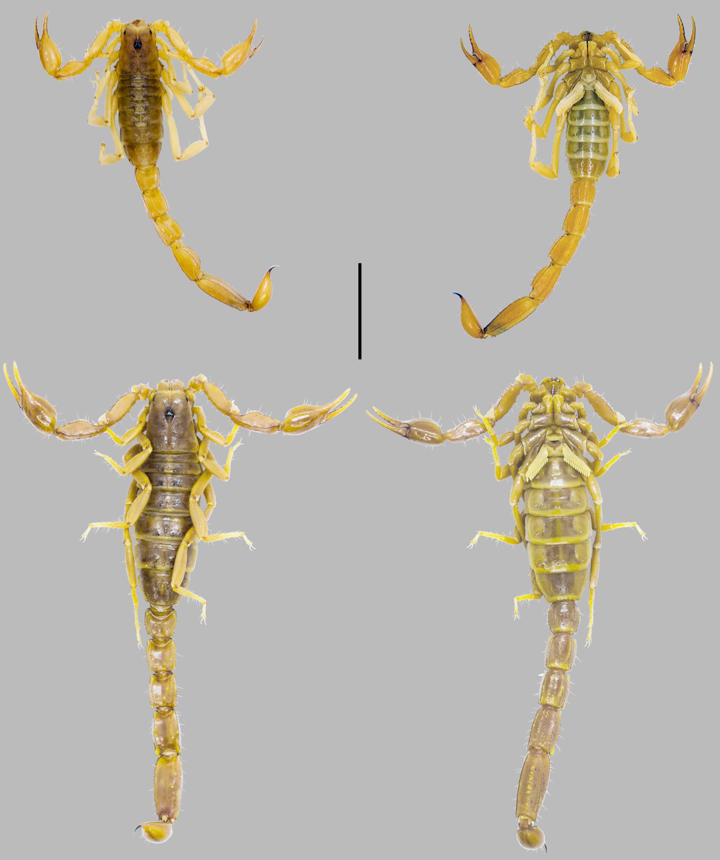
Figure 9. Habitus of male (top) and female (bottom) of C. glabrimanus, scale = 1 cm.
Chihuahuanus glabrimanus (Sissom & Hendrixson, 2005) (Fig. 9)
Taxonomic summary
Holotype: Florida State Collection of Arthropods, Gainesville, Florida, USA. México, Nuevo Léon: 7.8 km N La Ascension, 24°19’0.00” N, 99°54’00.00” W, 18-07-1972, E.A. Liner, R. M. Johnson, A. H. Chaney, 1 adult ♂. Paratype Mexico, Coahuila: 10.8 km S, 0.16 km E Arteaga at Los Pinos, 25°17’00.00” N, 100°50’00.00” W, 17-09-1975, leg. E.A. Liner et al.
Records from literature: González-Santillán and Prendini (2013): Mexico, Guanajuato, Municipality of San Diego de la Union: San Diego de la Unión, 8 km S, 21°23’08.67” N, 100°53’27.14” W, 2,078 m, 28-07-2006, E. González, M. Córdova, A. Jaimes, A. Ballesteros, O. F. Francke, 1 ♂, AMNH. San Luis Potosí, Municipality of Villa de Arista: Villa de Arista, 10 km E, 22°30’45.65” N, 100°45’29.99” W, 30-08-2006, O. F. Francke, W. D. Sissom, G. Casper, T. Anton, V. Torti, H. Montaño, C. Santibáñez, A. Ballesteros, 4 ♂ 1 ♀, CAS (ARA1909). González-Santillán and Prendini (2015): México, Guanajuato, Municipality of San Diego de la Unión: San Diego de la Unión, 8 km S, 21°23’08.64” N, 100°53’27.12” W, 2078 m, 28-07-2006, O. F. Francke, M. Córdova, A. Jaimes, E. González, A. Ballesteros, 1 juv. AMCC (LP 6611). Nuevo León, Municipality of Galeana: Providencia, 3 km E, 25°08’39.06” N, 100°39’02.40” W, 1,980 m, 17-07-2006, O. F. Francke, E. González, M. Córdova, J. Ballesteros, A. Jaimes, 1 ♂, AMCC (LP6558). San Luis Potosí, Muncipality of Ciudad del Maíz: Puerto Santa Catarina, 22°18’13.38” N, 99°37’16.08” W, 1,214 m, 22-08-2006, O. F. Francke, W. D. Sissom, G. Casper, T. Anton, V. Torti, H. Montaño, C. Santibáñez, A. Ballesteros, 1 juv, AMCC (LP6610).
Examined material: Mexico, Aguascalientes, Municipality of Aguascalientes: Jardín Botánico Rey Netzahualcoyotl, 10-08-2004, V., 1 ♂, CZUAA SCO-172; 8-06-, G. García, 1 ♂, CZUAA SCO-178; 8-01-2004, J. Escoto, 1 ♀, CZUAA SCO-180; 27-06-2015, J. E. Díaz-Plascencia, 1 ♂, 1 ♀, CZUAA SCO-183. Universidad Autónoma de Aguascalientes, edificio 1 A, 13-10-2015, M. Croce-Hernández, 1 ♀, CZUAA SCO-373; edificio 132, 28-08-2019, I. Villalobos-Juárez, 1 ♂, CZUAA SCO-469; 23-06-2015, G. De la Riva-Hernández, 1 ♀, CZUAA SCO-181; 21-09-2017, M. Martínez, 1 ♂, 1 ♀, CZUAA SCO-438. Avenida Circunvalación lado E, 24-11-1985, O. Rosales-Carrillo, 1 ♀, CZUAA SCO-170. Fraccionamiento Asturias, 18-12-2002, J. A. Escoto-Moreno, 1 ♂, CZUAA SCO-175. Carretera Aguascalientes-San Luis Potosí km 2.5, 15-08-2004, J. A. Escoto-Moreno, 1 ♂, 1 ♀, CZUAA SCO-171. Los Pericos, 29-05-2000, V. Herrera, 1 ♀, CZUAA SCO-165; 28-05-2000, R. M. Morales-Contreras, 1 ♀, CZUAA SCO-169. Rancho El Cocuyo, 23-10-1993, L. Delgado-Saldívar, 1 ♀, CZUAA SCO-173. Centro de Salud Urbano, colonia Guadalupe Peralta, 15-06- 2023, I. Martínez, 2 ♂, CZUAA SCO-734. Municipality of Asientos: Francisco Villa, hogar particular, 22°05’19.00” N, 101°58’05.00” W, 15-10-2002, F. Aguinaga, CNAN-SC4043. Municipality of Calvillo: Cercano a balneario “La Cueva”, 21°49’57.00” N, 102°48’58.82” W, 15-10-2019, F. Chávez-Samayoa, 1 ♀, CZUAA SCO-560. Presa Malpaso, 10-09-1985, C. Ortiz-de L., 1 ♀, CZUAA SCO-164; 1 ♀, 26-09-1993, J. M. González-Martínez CZUAA SCO-174. Municipality of Cosío: Soledad de Abajo, unidad médica, 25-10-2002, F. Aguinaga, CNAN-SC4044. Casa del centro, 1-01-2002, F. Aguinaga, CNAN-SC4045. Municipality of El Llano: Juan el Grande, 21°55’58.40” N, 101°55’42.49” W, 2,198 m, 8-08-2020, F. Chávez-Samayoa, 1 ♂, CZUAA SCO-523. Municipality of Jesús María: Los Arquitos, 21°55’21.68” N, 102°23’17.92” W, 4-09-2019, I. Villalobos-Juárez, F. Chávez-Samayoa, 1 ♀, CZUAA SCO-559. Buenavista, 11-06-2000, R. M. Muñoz, 1 ♂, CZUAA SCO-179. Municipality of Pabellón de Arteaga: Río San Pedro, 23-06-2015, J. L. Aguilar-Aguilar, 1 ♂, CZUAA SCO-182. Municipality of Tepezalá: Cerro del Capulín, 22°14’30.30” N, 102°09’30.13” W, 31-05-2020, I. Villalobos-Juárez, P. C. Hernández-Romero, D. F. Simijaca-Salcedo, F. Chávez-Samayoa, 1 ♂, CZUAA SCO-515; 22°14’16.19” N, 102°09’15.88” W, 6-06-2020, F. Chávez-Samayoa, 1 ♂, CZUAA SCO-542; 22°14’07.25” N, 102°09’25.16” W, 26-09-2020, F. Chávez-Samayoa, D. F. Simijaca-Salcedo, I. Villalobos-Juárez, 1 ♀, CZUAA SCO-563. Tepezalá, 21°13’54.41” N, 102°10’03.06” W, 2,116 m, 7-08-2015, M. Rodríguez. Guanajuato, Municipality of San Luis de la Paz: 7 km E of San Luis de la Paz, 21°18’42.84” N, 100°25’36.06” W, 2,117 m, 24-08-2006, O. F. Francke, H. Montaño, C. Santibáñez, A. Ballesteros, 2 ♂, CNAN-SC02455. Nuevo León, Municipality of Galeana: Carretera San Roberto-Galeana, km 78, 24°40’57.6” N, 100°06’24.0” W, 1,944 m, O. F. Francke, W. D. Sissom, K. McWest, B. Hendrixson, S. Grant, E. González S., M. Córdova, A. Jaimes, A. Ballesteros, 1 ♀, CNAN-SC2136. Providencia, 3 km NE, 25°08’39.06” N, 100°39’02.40” W, 1,980 m, 17-07-2006, O. F. Francke, E. González, M. Córdova, J. Ballesteros, A. Jaimes, 1 ♂, AMCC (LP 6558). 3km NW of La Providencia, 25°08’39.12” N, 100°39’02.88” W, 1,980 m, 17-07-2006, O. F. Francke, E. González, A. Jaimes, M. Córdova, A. Ballesteros, 5 ♂, CNAN-SC3108. Querétaro: Estación de Microondas Santa Lucia hacia Peña Miller, matorral espinoso, 21°03’28.30” N, 99°47’01.90” W, 13-11-2009, O. F. Francke, J. Cruz-López, C. Santibáñez, A. Valdez, 1 ♀ juv., CNAN-SC2133. San Luis Potosí, Municipality of Ciudad del Maíz: Puerto Santa Catarina, 22°18’13.38” N, 99°37’16.08” W, 1,214 m, 22-08- 2006, O. F. Francke, W. D. Sissom, G. Casper, T. Anton, V. Torti, H. Montaño, C. Santibáñez, A. Ballesteros, 1 juv., AMCC (LP 6610). Municipality of Villa de Arista: 10 km E of Villa de Arista, 22°38’45.60” N, 100°45’29.94” W, 1,624 m, 20-08-2006, O. F. Francke, D. W. Sissom, T. Anthon, V. Totti, G. Casper, H. Montaño, C. Santibáñez, A. Ballesteros, 2 ♂, CNAN-SC03107. Zacatecas, Municipality of Fresnillo: 23-05-2009, S. R. López-Navarro, 1 ♀, CZUAA SCO-168; 21-06-2009, R. López-Navarro, 1 ♂, CZUAA SCO-176. Municipality of Jalpa: 15-04-2005, J. Silva, 1 ♀, CZUAA SCO-167. Municipality of Saín Alto: Emiliano Zapata, 9-09-1971, S. Guijosa, 1 ♀, CNAN SC02456.
Remarks
Chihuahuanus glabrimanus is distributed in Aguas-calientes, Coahuila, Guanajuato, Nuevo León, Querétaro, and San Luis Potosí (González-Santillán & Prendini, 2013, 2015).This speciesexhibits somewhat variable external morphology but is not correlated with its distribution, complicating its separation into morphospecies. Unlike diplocentrids, C. glabrimanus and C. coahuilae present some degree of substrate-specialism, having more and less elongated and alienated setae on the telotarsi, which is characteristic of the psammophilic ecomorphotype, an adaptation to digging in sandy soils (Polis, 1990; Prendini, 2001). Although we collected specimens in sandy areas, we failed to find a significant relationship between their presence and sandy habitats.

Figure 10. Habitus of male (top) and female (bottom) of M. spadix, scale = 1 cm.
Mesomexovis spadix (Hoffmann, 1931) (Fig. 10)
Taxonomic summary
Holotype: deposited in the American Museum on Natural History, New York, USA. México, Zacatecas, Municipality of Jalpa, 1 ♂, paratypes same locality deposited in UNAM 053, 1 ♂, 1 ♀ (Sissom, 2000).
Records from literature: González-Santillán & Prendini (2013): México, Guanajuato, Municipality of León: León, -04-2004, P. Berea, 1 ♂, 1 ♀, CNAN. Hoffmann (1931): México, Zacatecas, Jalpa. Santibáñez-López et al. (2015): México, Aguascalientes, Jalisco, Zacatecas. Sissom (2000): México, Aguascalientes, Jalisco, Zacatecas.
Examined material: Mexico, Aguascalientes, Municipality of Aguascalientes: Cerro de Los Gallos, 16-09-2014, J. E. Díaz-Plascencia, 2 ♀, CZUAA SCO-197; 27-11-1997, V. Villalobos-Sánchez, 1 ♀, CZUAA SCO-289; 26-11-1984, H. Gallegos-Rangel, 2 ♀, CZUAA SCO-295; 21-10-1989, M. E. Serafín-Luevano, 2 ♂, CZUAA SCO-297; -04-2015, C. A. Franco-Servín de la Mora, 2 ♀, CZUAA SCO-316. Cerro del Muerto, 23-05-2014, E. A. Hernández-Medrano, 1 juv. ♂, CZUAA SCO-248; 14-06-1979, J. Á. Uyoa, 1 ♀, CZUAA SCO-259; 10-04-2010, L. Consuelo-Márquez, 1 ♀, CZUAA SCO-268; 19-10-1988, J. A. Rodríguez-Avalos, 3 ♂, 4 ♀, CZUAA SCO-275; 21-10-1982, M. E. Serafín-Luevano, 2 ♂, CZUAA SCO-297. El Sauz, km 35, 19-04-1996, F. Arenas-Luevano, 1 ♂, CZUAA SCO-227. Municipality of Calvillo: Peña Blanca, 21°54’09.76” N, 102°45’15.48” W, 31-01-2022, I. J. Rodríguez-Elizalde, J. Brito-Ruiz de Velasco, 1 ♂, CZUAA SCO-724. Sierra Escondida, 21°43’32.12” N, 102°43’14.52” W, 10-02-2022, I. J. Rodríguez-Elizalde, J. Brito-Ruiz de Velasco, 1 ♂ juv., CZUAA SCO-725. 7 km NE of Temazcal, 22°02’36.46” N, 102°44’07.22” W, 2,246 m, 6-09-2021, I. J. Rodríguez-Elizalde, J. Brito-Ruiz de Velasco, 1 ♀, CZUAA SCO-682. Cercano a balneario “La Cueva”, 21°49’57.00” N, 102°48’58.82” W, 1,781 m, 28-10-2019, F. Chávez-Samayoa, S. S. Gutiérrez-Martínez, 1 ♀, CZUAA SCO-482; 15-10-2019, F. Chávez-Samayoa, 6 ♂, 22 ♀, CZUAA SCO-485. Los Adobes, 21°48’39.22” N, 102°41’21.34” W, 1,874 m, 11-10-2019, F. Chávez-Samayoa, L. R. Haro-Tapia, 2 ♀, CZUAA SCO-487. La Mezquitera, 21°51’39.85” N, 102°46’03.47” W, 5-10-2019, F. Chávez-Samayoa, M. E. Samayoa-Sepúlveda, L. F. Chávez-Rodríguez, 2 ♀, CZUAA SCO-511; 7-09-2019, F. Chávez-Samayoa, 7♂, 5♀, CZUAA SCO-513; 30-08-2019, J. A. Escoto-Moreno, F. Chávez-Samayoa, 4 ♀, CZUAA SCO-592. Presa La Codorniz, 21°59’50.78” N, 102°40’42.78” W, 2,068 m, 5-07-2021, F. Chávez-Samayoa, D. Ortiz-Álvarez, C. Huerta, 10 ♂, 12 ♀, CZUAA SCO-613; 22°00’39.07” N, 102°40’19.51” W, 1-11-2020, E. González-Martínez, J. L. Reyes-Hernández, I. E. Gallegos-Vieyra, D. F. Simijaca-Salcedo, F. Chávez-Samayoa, 1 ♀, CZUAA SCO-590. Presa Los Alamitos, 21°43’49.44” N, 102°42’50.04” W, 14-06-2021, M. E. Samayoa-Sepúlveda, F. Chávez-Samayoa, 1 ♀, CZUAA SCO-635; 17-05-2021, F. Chávez-Samayoa, D. Ortiz-Álvarez, 1 ♀, CZUAA SCO-649; 13-02-2021, D. G. Castillo-Arceo, N. D. Morales, 1 ♀, CZUAA SCO-663. Los Alisos, 4-03-2005, M. Orozco, 1 ♀, CZUAA SCO-311. El Ocote, 13-06-2009, M. Gómez, 1 ♀, CZUAA SCO-208; 11-06-2004, G. Guerrero, 1 ♀, CZUAA SCO-215; 12-06-2004, Benjamín, 1 ♀, CZUAA SCO-217; 13-06-2004, A. Del Río, 1 ♀, CZUAA SCO-255; 13-06-2004, S. Saucedo, 1 ♀, CZUAA SCO-267; -06-2002, E. N. Manzo-Mata, 2 ♀, CZUAA SCO-284; 13-06-2004, R. S. Pérez, 1 ♂, 1 ♀, CZUAA SCO-293. El Pilar, 2-05-2004, P. O. Hernández, 1 ♀, CZUAA SCO-214. La labor, caseta de vigilancia, 17-06-1992, J. A. Castorena Rangel, 1 ♀, CZUAA SCO-260. Las lomas, 3.5 km hacia Presa de los Serna, 14-10-1992, H. J. Cruz-González., 1 ♂, 1 ♀, CZUAA SCO-256. Las moras, 15-03-2007, S. Álvarez-Betancourt, 1 ♀, CZUAA SCO-442. Los Alisos, 12-09-1988, J. A. Rodríguez-Avalos, 2 ♀, CZUAA SCO-219; 22-01-2014, A. Farfán-Castañeda, 1 ♂, CZUAA SCO-224; 19-05-1982, V. Quintero, A. Salado, 2 ♂, CZUAA SCO-231; 9-10-1989, M. Y. Quezada, J. I. Soriano, 4 ♂, 4 ♀, CZUAA SCO-294; 3-10-2014, J. E. Díaz-Plascencia, 2 ♀, CZUAA SCO-417. Presa Malpaso, 13-06-2004, Hernández-Camacho, 1 ♀, CZUAA SCO-210; 1-06-2005, C. C. Herrada, 2 ♂, 3 ♀, CZUAA SCO-225; 13-06-2004, E. J. Ortiz-Martínez, 1 ♀, CZUAA SCO-244; 13-06-2004, L. Muro, 2 ♀, CZUAA SCO-250. Mesa Montoro, 4-05-1996, F. Arenas-Luevano, 1 ♀, CZUAA SCO-291. Río Gil, 11-06-2004, A.E.G.E., 2 ♀, CZUAA SCO-296. Sierra del Laurel, 18-04-2010, A. G. Pérez D., 1 ♀, CZUAA SCO-237; 29-08-2015, J. E. Díaz-Plascencia, 4 ♂, 3 ♀, CZUAA SCO-319; 11-02-2017, V. M. Arano-Sierra, 1 ♂, CZUAA SCO-415. Municipality of El Llano: Juan el Grande, 21°56’21.00” N, 101°55’06.00” W, 18-10-2019, F. Chávez-Samayoa, E. González-Martínez, 1 ♂, 1 ♀, CZUAA SCO-476; 21°56’22.45” N, 101°55’22.22” W, 23-08-2020, F. Chávez-Samayoa, 1 ♀, CZUAA SCO-534; 21°56’21.08” N, 101°55’17.87” W, -10-2019, E. González-Martínez, 6 ♂, 5 ♀, CZUAA SCO-544; 21°56’20.00” N, 101°55’09.84” W, 2,488 m, 27-02-2021, F. Chávez-Samayoa, D. F. Simijaca-Salcedo, 1 ♂, CZUAA SCO-642. Municipality of Jesús María: Los Muñozes, 21°57’00.14” N, 102°34’00.66” W, 2,179 m, 12-10-2019, F. Chávez-Samayoa, M. J. Morán-Gutiérrez, V. M. Arano-Sierra, 3 ♂, 9 ♀, CZUAA SCO-478; 16-10-2019, F. Chávez-Samayoa, 2 ♂, 7 ♀, CZUAA SCO-479. Los Arquitos, 21°55’21.68” N, 102°23’17.92” W, 1,931 m, 4-09-2019, F. Chávez-Samayoa, 6 ♂, 22 ♀, CZUAA SCO-485; 4-09-2019, I. Villalobos-Juárez, 4 ♀, CZUAA SCO-512; 21°55’12.51” N, 102°23’47.53” W, 2,034 m, F. Chávez-Samayoa, D. F. Simijaca-Salcedo, 3 ♀, CZUAA SCO-639; 21°55’18.66” N, 102°23’34.79” W, 1,964 m, 26-03-2021, F. Chávez-Samayoa, D. F. Simijaca-Salcedo, 2 ♀, CZUAA SCO-640. Pileta, 21°57’20.92” N, 102°30’02.92” W, 2,167 m, 6-09-2019, J. A. Escoto-Moreno, F. Chávez-Samayoa, 1 ♀, CZUAA SCO-593. Campamento Yuca, 22°02’20.37” N, 102°24’43.12” W, 2,262 m, 7-10-2019, M. J. Perales-Olivares, 1 ♀, CZUAA SCO-465. Cerro El Picacho, 18-10-1986, P. Serna-Pérez, 1 ♀, CZUAA SCO-263; 13-11-1985, J. G. Vázquez A., 1 ♀, CZUAA SCO-267; -08-2020, C. Ramírez, 1 ♀, CZUAA SCO-587. La Posta, 5-06-2014, E. Águila-Lira, 1 ♂, CZUAA SCO-236. Rancho Seco, 21-04-2019, V. M. Arano-Sierra, 1 ♂, 1 ♀, CZUAA SCO-472. Municipality of Pabellón de Arteaga: 25-06-1999, C. A. Ramírez, 1 ♀, CZUAA SCO-228. Municipality of Rincón de Romos: Sierpe, Y. Calvillo Lezama, 1 ♂, 1 ♀, CZUAA SCO-298. Rincón de Romos, 17-04-2004, N. Arroyo-Chávez, 1 ♂, CZUAA SCO-243; 20-06-1999, P. Hernández, 1 ♀, CZUAA SCO-258; 20-11-1999, L. F. de Alba, 1 ♀, CZUAA SCO-271; 23-03-1999, B. Saucedo, 1 ♀, CZUAA SCO-274. Municipality of San Francisco de los Romo: 6-06-2016, A. Bernal, 1 ♀, CZUAA SCO-446. Municipality of San José de Gracia: Estación Biológica Agua Zarca, 22°05’32.3” N, 102°33’20.3” W, 2,149 m, 20-03-2019, E. C. Ramírez, 1 ♂, 4 ♀, CZUAA SCO-547; 12-03-2003, Y. Gámez-Roldán, 1 ♂, CZUAA SCO-198; -02-2003, A. Morales, 1 ♀, CZUAA SCO-201; 18-03-2003, C. Quiñones-Valles, 1 ♀, CZUAA SCO-203; 29-03-2003, C. A. Morales-Asencio, 1 ♀, CZUAA SCO-204; 30-03-2014, J. Montero, 1 ♀, CZUAA SCO-211; 5.-04-2014, J. E. Díaz-Plascencia, 1 ♂, 2 ♀, CZUAA SCO-213; 31-05-2014, F. Chávez-Samayoa, 1 ♀, CZUAA SCO-238; 31-05-2014, R. González-Muñoz, 1 ♀, CZUAA SCO-241; -02-2003, A.P.R.A., 1 ♂, CZUAA SCO-288; 30-05-2014, A. Mejía-Arellano, 1 ♂, CZUAA SCO-314; 28-04-2004, L. Rodríguez, 1 ♀, CZUAA SCO-315; 13-05-2016, O. Herrera, 1 ♀, CZUAA SCO-406; 20-05-2016, L. R. Haro-Tapia, 1 ♂, CZUAA SCO-409; 18-05-2018, F. S. Álvarez-Solís, 1 ♀, CZUAA SCO-414; 27-05-2016, I. Rodríguez-Ortiz, 1 ♀, CZUAA SCO-428. Guanajuato, Municipality of León: Colonia La Luz, V. H. González, 1 ♂, CZUAA SCO-230; León, 25-06-2007, M. Ávila, 1 ♀, CZUAA SCO-410. Municipality of Guanajuato: 26-05-2007, D. García, 1 ♀, CZUAA SCO-426. Municipality of Salamanca: J. A. Berlín-Diosdado, 1 ♀, CZUAA SCO-226. Jalisco, Municipality of Lagos de Moreno: Cerro La Bola, 18-02-2012, R. E. Rea-Reyes, 1 ♀, CZUAA SCO-222. Lagos de Moreno, 24-04-2016, C. E. Valdivia-Muñoz, 1 ♀, CZUAA SCO-451. Municipality of Guadalajara: 6-06-2017, O. Gutiérrez-Muñoz, 1 ♂, 1 ♀, CZUAA SCO-423. Zacatecas, Municipality of Guadalupe: Cerro de la Virgen, 1-06-2003, C. A. Barrón, 1 ♀, CZUAA SCO-262. Municipality of Jerez de García: Sierra de Los Cardos, 14-10-2015, R. A. Rosales-García, 1 ♂, 1 ♀, CZUAA SCO-313. Cerro de la Campana, 17-03-2014, R. A. Rosales-García, 1 ♂, 1 ♀, CZUAA SCO-209. Jerez, 2-11-1986, R. Macías-Ramírez, 1 ♀, CZUAA SCO-234. Municipality of San Pedro Piedra Gorda: Chiquihuitillo, 22-09-1990, M. G. Flores Olivares, 1 ♂, CZUAA SCO-245.
Remarks
Mesomexovis spadix occurs in Aguascalientes, Guanajuato, Jalisco, and Zacatecas (González-Santillán & Prendini, 2013; Hoffmann, 1931; Santibáñez-López et al., 2015; Sissom, 2000).
Hoffmann (1931) synonymized Vaejovis punctatus spadix and Vaejovis punctatus variegatus Pocock, 1898 with Vaejovis punctatus punctatus, although he recognized some differences, he did not consider them enough to separate species. Later, González-Santillán and Prendini (2013) erected Mesomexovis and elevated them to species rank as M. spadix and Mesomexovis variegatus. Some authors have enlisted Mesomexovis punctatus as part of Aguascalientes species richness (Ponce-Saavedra & Francke, 2013b; Contreras-Félix et al., 2015), probably confounding the former nominotypical subspecies.
Mesomexovis spadix is a very abundant lapidicolous species covering most of the territory of Aguascalientes and tolerates disturbed environments. We collected specimens in 7 of the 11 municipalities of the state: Aguascalientes, Calvillo, El Llano, Jesús María, Pabellón de Arteaga, Rincón de Romos, and San José de Gracia. Although M. spadix occupies the 3 biogeographical provinces in Aguascalientes, the Chihuahuan desert appears to limit its distribution to the northern territories, which is congruent with the prediction of González-Santillán and Prendini (2013), who mentioned that Chihuahuanus ecologically substitutes Mesomexovis in more arid areas.

Figure 11. Habitus of male (top) and female (bottom) of T. intrepidus, scale = 1 cm.
Thorellius intrepidus (Thorell, 1876) (Fig. 11)
Taxonomic summary
Holotype: deposited in the Naturhistoriska Riksmuseets Stockholm, Sweden. The only information associated to the holotype is: México 1 ♀ (Sissom, 2000).
Records from literature: González-Santillán and Prendini (2013): México, Colima, Municipality of Armería: Mine la Salada, NW Ixtlahuacan, 19°01’40.85” N, 103°47’02.21” W, 275 m, mine staff, 1 ♂, 1 ♀, AMNH. Municipality of Tecomán: Tecomán, 18°54’30.00” N, 103°52’28.00” W, 1 ♂, 1 ♀, AMNH. González-Santillán & Prendini (2018): México, Aguascalientes, Municipality of Calvillo: Chiquihuitero, 21°52’27” N, 102°42’09” W, 1,680 m, 29-06-2007, A. Valle Colis , 1 ♂, INDRE; El Rodeo, 21°52’09” N, 102°44’50” W, 1,620 m, 25-06-2007, A. Valle Colis, 1 ♀, INDRE; La Labor, 21°57’43” N, 102°41’46” W, 1,740 m, 15-18-06-2007, I. Escalante-Piña, 1 ♂, 1 ♀, INDRE; Rancho Media Luna, 21°47’56” N, 102°48’05” W, 1,560 m, 9-11-2008, I. Franchini, 1 ♀, INDRE; Mesa Grande, 21°48’18” N, 102°43’18” W, 1,760 m, 24-06-2003, G. Vargas, 1 ♀, INDRE, 24-06-2007, M. Sema, 1 ♂, INDRE. Colima, Municipality of Armeria: Armeria, 18°56’03” N, 103°57’52” W, 40 m, 2-01-2003, H. Rodríguez, 1 ♂, 1 ♀, CNAN SC2628. Mina La Salada, NW Ixtlahuacán, at mine headquarters, 19°01’40.80” N, 103°47’02.16” W, 275 m, 2005, mine staff, 11 ♀, AMNH. Municipality of Camotlán: Punta de Agua, 19°09’00.00” N, 104°16’00.00” W, 2-09-2003, E. González, 1 ♀, CNAN SC2242. Municipality of Colima: Colima, 19°14’36.00” N, 103°43’28.98” W, 30-12-1927, J. C. Chamberlin, 1 ♂, AMNH. Colima, 16 km S, 19°14’37” N, 103°43’51” W, 30-07-1954, W. J. Gertsch, 1 ♂, AMNH. Los Ortices, 19°06’46.8” N, 103°44’22.6” W, 343 m, 9-04-2004, P. Berea, 1 ♂, AMCC (LP 6379). Municipality of Comala: Comala, 19°19’00.00” N, 103°45’00.00” W, 9-04-2004, P. Berea, 1 juv. ♀, AMCC (LP 6377). Municipality of Coquimatlán: near Coquimatlán, 19°18’00.00” N, 104°06’00.00” W, 2008, L. L. Valdez, 1 ♂, CNAN SC2921. Municipality of Manzanillo: Los Parajes, 19°14’07” N, 104°24’52” W, 230 m, 3-02-2008, 1 ♂, INDRE. Manzanillo, 19°03’08” N, 104°18’57” W, 5 m, 1 ♀, INDRE, 17-01-1947, 2 ♂, 4 ♀, 1 subad. ♂CNAN SC2634. Manzanillo, 10 km of El Colomo, 19°03’08” N, 104°18’57” W, 16-04-2008, P. Berea, 1 ♀, CNAN SC2619. Colonia Valle de Las Garzas, 19°03’08” N, 104°18’57” W, 29-09-2008, 5 m, 1 ♀, INDRE. Manzanillo, Sector 7, 19°03’08” N, 104°18’57” W, 5 m, 6-02-2004, 1 ♂, INDRE. Nuevo Petatero Ranch, 19°03’38.94” N, 104°16’36.12” W, 4-02-2008, 1 ♀, INDRE. Potrero Grande, 19°10’19” N, 104°32’27” W, 6 m, 27-11-2008, 1 ♀, INDRE. Veladero de Otates, 19°15’38” N, 104°20’14” W, 280 m, 4-02-2008, 1 ♀, INDRE. Municipality of Minatitlán: Junction to Saus, on way to Minatitlán, 19°25’22.74” N, 103°58’59.94” W, 1,006 m, 26-05-2006, O. F. Francke, A. Valdez, H. Montaño, A. Ballesteros, 1 ♂, AMCC (LP 6469). Municipality of Tecomán: Tecomán, 18°54’30” N, 103°52’28” W, 8-05-1961, E. López, 1 subad. ♀, INDRE, -03-1992, Orozco, R. G., 1 ♂, INDRE, 30 m, 9-03-1992, R. Lezama, 3 ♂, 6 ♀, CNAN SC2629, around village, 29-11-1995, E. López, 1 ♀ 1 subad. ♂, CNAN SC2611, 12-01-1996, M. González, 1 ♀, CNAN SC2605, 18-02-1996, H. Arredondo, 1 ♀, CNAN SC2641, 19-06-1996, H. Arredondo, 1 ♀, INDRE. Municipality of Villa de Álvarez: Villa de Álvarez, 19°16’00.00” N, 103°44’15.00” W, 530 m, 11-02-1995, E. Polanco, 1 ♀, CNAN SC2618. Guanajuato, Municipality of León: Hacienda de Arriba, NE of León, in house, 2008, L. Olguín, 2 ♀, CNAN SC2922; León, 21°07’00.00” N, 101°41’00.00” W, 2-06-2006, 1 ♂, CNAN SC2612. Jalisco, Municipality of Jocotepec: San Juan Cosola, 1.6 km E, 20°17’12.00” N, 103°20’13.02” W, 10-07-1959, C. M. Bogert, 1 ♀, AMNH. Muncipality of La Huerta: Ejido E. Zapata, 19°22’58” N, 104°57’55” W, 10 m, 9-07-1994, I. Ramírez, 1 ♀, CNAN SC2606. Estación Biológica Chamela, 19°29’52.50” N, 105°02’36.48” W, 5-04-1981, M. V. Julia, 1 ♀, CNAN-SC2244, 20 m, 19-05-1985, A. Pescador, 1 subad. ♀, CNAN-SC2607; 26-04-1993, E. Ramírez, 1 ♂, CNAN SC2614; 25-03-1998, S. H. Bullock, 1 ♀, CNAN-SC2920; 14-09-1999, A. M. Corona, R. Ayala, 1 ♀, CNAN-SC2621; 19-09-1999, A. M. Corona, 1 ♀, CNAN-SC2622; 1-09-2011, O. F. Francke, A. Valdez, H. Montaño, A. Ballesteros, C. Santibáñez, 3 ♂, 1 ♀, CNAN-SC2245; 19°29’52.50” N, 105°02’36.48” W, 97 m, 30-08-2007, O. Francke et al., 1 juv. ♀, AMCC (LP 7670); Estación Biológica Chamela, El Tejon Trail, 19°29’50.16” N, 105°02’29.46” W, 18-08-2005, J. L. Castelo, UV detection at night, 1 juv., AMCC (LP 5309). Michoacán, Municipality of Aquila: Aquila, 18°35’57” N, 103°30’15” W, 180 m, 21-02-1992, R. Mares, 1 ♀, CNAN-SC2636. Arroyo de la Cruz, 5 km NE of Maquili, 18°34’33.5” N, 103°35’47.8” W, 24-01-2004, 1 ♂, 2 ♀ 1 subad. ♂ 1 subad. ♀, CNAN-SC2992. El Faro de Bucerías, tropical dry forest, 18°21’00.00” N, 103°29’00.00” W, 13/14-01-2002, E. González, 1 ♀, AMCC (LP 2022); El Faro de Bucerías, near La Llorona 18°20’40.74” N, 103°30’32.04” W, 17-01-2006, G. Suárez, CNAN-SC2624. Pomaro, 18°20’28” N, 103°18’29” W, 380 m, 1 ♂, 18-02-1992, R. Álvarez, 1 ♀, CNAN-SC2608. Municipality of Coahuayana: Coahuayana, 18°45’00.00” N, 103°40’00.00” W, 24-06-1991, M. J. Nereida, 1 ♀, CNAN-SC2615. Municipality of Jiquilpan: Jiquilpan, 19°59’37” N, 102°43’02” W, 1,560 m, G. Ignacio, 1 ♂, 1 ♀, CNAN-SC2616. University of Michoacán, 19°41’27.96” N, 101°12’09.78” W, 1 ♂, CNAN-SC2613. Municipality of Uruapan: Uruapan, 19°25’10” N, 102°03’30” W, 1,620 m, J. Julia, 1 ♂, CNAN-SC2610. Nayarit, Municipality of Tepic: La Loma motel, 21°30’30.00” N, 104°53’34.98” W, C.M. Bogert, 1 ♀, AMNH. Santibáñez-López et al. (2019): México, Colima, Municipality of Coquimatlán: El Palapo, 19°11’54.60” N, 102°54’49.68” W, 3-04-2015, J. Valencia, J. López, E. González. Soleglad & Fet (2008): México, Nayarit, Municipality of Tepic: 1 ♀, MES, 1 ♀, GL.
Examined material: Mexico, Aguascalientes, Municipality of Calvillo: Calvillo, 9-06-2021, I. J. Rodriguez-Elizalde, 1 ♂, CZUAA SCO-609. Terrero de la Labor, 22°01’32.02” N, 102°39’58.00” W, 1,927 m, 22-10-2021, F. Chávez-Samayoa, D. Ortiz-Álvarez, 1 ♀, CZUAA SCO-656. Presa de los Serna, 3-10-2003, S. García, 1 ♀, CZUAA SCO-188; 3-10-2003, S. García, 1 ♂, CZUAA SCO189. Calvillo, 8-11-2021, R. García, 1 ♂, CZUAA SCO-669. Jalisco, Municipality of Encarnación de Diaz: 5-06-2009, E. Duar, 1 ♀, CZUAA SCO-378. Municipality of San Juan de los Lagos: 14-04-2011, F. A. Rubalcaba-Castillo, 1 ♀, CZUAA SCO-194.
Remarks
Thorellius intrepidus inhabits the states of Aguascalientes, Colima, Guanajuato, Jalisco, Michoacán, and Nayarit, inhabiting tropical dry forests, deciduous and broadleaf forests between 5 and 1,760 m altitude (González-Santillán & Prendini, 2018).
In Aguascalientes, we recorded T. intrepidus at 1,927 m of altitude (CZUAA SCO-656), which may represent most likely its altitudinal distribution limit at circa 2,000 m. Thorellius intrepidus is restricted to the tropical deciduous forest of the Calvillo Municipality. Like C. infamatus, T. intrepidus inhabits the Pacific Lowlands province, which may be a second component that invaded or diversified within that area. However, all the species of Thorellius are distributed in tropical to subtropical habitats (González-Santillán & Prendini, 2018) connected to the Pacific Lowlands, which suggest that the linage may have originated in the Pacific Lowlands province.
Smeringurinae Soleglad & Fet, 2008

Figure 12. Habitus of male (top) and female (bottom) of P. gracilior, scale = 1 cm.
Paruroctonus gracilior Hoffmann, 1931 (Fig. 12)
Taxonomic summary
Lectotype: deposited in the American Museum of Natural History, New York, USA. Tepezalá, Aguascalientes, México, 1 ♂ and 2 paralectotypes ♂♂.
Records from literature: Brown et al. (2002): USA, Texas, Terrel County: Chandler Independence Creek Preserve, 30°26’30.00” N, 101°43’26.00” W. Bryson Jr. (2014): USA, Arizona, Cochise County. Fet et al. (2006): México, Coahuila, Municipality of Cuatro Ciénegas: 2 ♂, MES. USA, New Mexico, Hidalgo County: Lordsburg, 1 ♂, GL. Gertsch & Soleglad (1966): México, Aguascalientes, Municipality of Tepezalá: C. C. Hoffmann, 3 ♂ cotypes, AMNH. Coahuila, Municipality of Saltillo: 32.1 km E of Saltillo, 16-07-1965, W. J. Gertsch, V. Roth, 1 ♂. USA, Arizona, Cochise County: Portal, 1-07- to 4-09-1965, R. M. Hastings, W. J. Gertsch, V. Roth, 27 ♂, 4 ♀. New Mexico, Hidalgo County: Rodeo, 29-08-1964, R. Hastings, 1 ♂. Eddy County: Hope, 23-09-1950, W. J. Gertsch, 1 ♀. Hoffmann (1931): México, Aguascalientes, Municipality of Tepezalá: 4 ♀. Sissom & Francke (1981): USA, New Mexico, Chaves County: 30.8 km W Caprock, 21-03-1980, J. E. Cokendolpher, 1 ♀, JCC. Eddy County: Carlsbad Caverns National Monument, 8-09-1969, M. A. Cazier, J. Bigelow, 4 ♂, 5 ♀, AMNH. 24.1 km E Loving (creosote scrub and dunes), -07-1978, C. Rudoph, 9 ♂, AMNH. Hidalgo County: 20.9 km N Rodeo, 25-06-1973, O. F. Francke, 2 imm., AMNH. Hope, 23-09-1950, W. J. Gertsch, 1 ♀. Rodeo, 29-08-1964, R. Hastings, ♂. Luna County: Rock Hound State Park, 14.4 km E Deming, J. Bigelow, 1 ♂, 1 ♀, AMNH. Texas, Brewster County: Castolon, Big Bend National Park, 8-08-1979, O. F. Francke, J. V. Moody, F. Merickel, 1 ♂, AMNH; Grapevine Ranch, N base of Grapevine Mountain, Big Bend National Park, 7-09-1969, M. A. Cazier, J. Bigelow, 15 ♂, 3 ♀, 2 imm, AMNH. Culberson County: 1.6 km N Kent, 23-06-1970, M. A. Cazier, L. Welch, O. F. Francke, 4 ♀, 3 imm., AMNH. Jeff Davis County: Panthon Spring, 25-06-1968, J. C. Lewis, 1 ♀, AMNH. 5.3 km N Presidio, 2-09-1972, J. Davidson, O. F. Francke, 8 ♂, 11 ♀, AMNH. 4.6 km E Presidio, 2-09-1972, J. Davidson, O. F. Francke, 6 ♂, 3 ♀, 1 imm., AMNH. 57.9 km S Marfa, 2-05-1980, L. Robbins, 2 juv., AMNH. Val Verde County: 0.8 km S Langry, 14-06-1974, L. Draper, A. Cazier, O. F. Francke, 1 ♀, AMNH. Winkler County: 4.8 km W Wink, 7.-04-1979, W. D. Sissom, 2 ♂, WDS. Soleglad and Fet (2008): México, Coahuila, Municipality of Cuatro Ciénegas: 1 ♂ 1 ♀, MES. USA, New Mexico: 1 ♂, MES. Texas, Brewster County: Lajitas, 1 ♂, GL. Stockwell (1986): USA, Texas, Brewster County: 4 km S of Alpine, 19-08-1968, S. C. Williams, J. Bigelow, M. M. Bentzien, 1 ♂, CAS. Big Bend National Park Grapevine Ranch, N base of Grapevine Mt., 7-09-1969, J. Bigelow, M. A. Cazier, 19 ♂, 5 ♀, AMNH; Big Bend National Park, 19.3 km SE Panther Jct., 17-08-1968, S. C. Williams, M. A. Cazier, 3 ♂, 3 ♀, CAS. 21.2 km SE of Panther Jct., 17, 17-08-1968, S. C. Williams, M. M. Bentzien, 14 ♂, 10 ♀, CAS. Big Bend National Park, Castalon, 8-08-1979, O. F. Francke, J. V. Moody, 1 ♂, AMNH. Crockett County: 10 mi. N of Iraan, 8-03-1986, S. A. Stockwell, J. M. Steele, 2 ♂, 4 ♀, SAS. Culberson County: 19.3 km E of Van Horn, 3-07-1965, M. H. Muma, 1 ♀, CAS. 1.6 km N of Kent, 25-06-1970, M. A. Cazier, Welch, O. F. Francke, 3 ♂, 4 ♀, AMNH. Hudspeth County: 12.8 km W of Van Horn, 11-06-1982, W. D. Sissom, 1 ♀, AMNH. Jeff Davis County: Phantom Springs, 25-06-1968, J. C. Lewis, 1 ♀, AMNH. Pecos County: 16.1 km N, 3 mi. W of Fort Stockton, 6-08-1967, W. L. Minckley, 1 ♂, CAS. Presidio County: Candelaria, 26-09-1977. R. Wilson, et al., 2 ♂, 1 ♀, CAS. 57.9 km S of Marfa, 2-05-1980, L. Robbins, 2 ♀, MWSU. 11.26 km N of Presidio, 27-11-1975, J. C. Cokendolpher, 1 ♀, MWSU. 5.3 km N of Presidio, 2.ix.1972, J. Davidson, O. F. Francke, 10 ♂, 11 ♀, AMNH. Val Verde County: 0.8 km S of Langtry, 14-06-1974, L. Draper, M. A. Cazier, O. F. Francke, 1 ♀, AMNH.
Examined material: Mexico, Aguascalientes, Municipality of Tepezalá: Cerro del Capulín, 22°14’30.30” N, 102°09’30.13”, 2159 m, 31-05-2020, F. Chávez-Samayoa, D. F. Simijaca-Salcedo, P. C. Hernández-Romero, 1 ♂, CZUAA SCO-517; 22°14’16.19” N, 102° 09’15.88” W, 2,138 m, 29-06-2020, F. Chávez-Samayoa, 1 ♀, CZUAA SCO-521; 22°14’06.83” N, 102°09’15.77” W, 2,130 m, 21-08-2020, F. Chávez-Samayoa, 2 ♂, 3 ♀, CZUAA SCO-539; 22°14’07.25” N, 102° 09’25.16” W, 2,117 m, 26-09-2020, F. Chávez-Samayoa, 1 ♀, CZUAA SCO-562; 22°13’52.88” N, 102°09’36.77” W, 2,127 m, 23-10-2020, I. Villalobos-Juárez, F. Chávez-Samayoa, D. F. Simijaca-Salcedo, 1 ♂, CZUAA SCO-576. San Luis Potosí, Municipality of Charcas: 23°16’00.36” N, 100°54’06.06” W, 2,029 m, -08-2010, O. F. Francke, D. W. Sissom, T. Anthon, G. Casper, V. Totti, H. Montaño, C. Santibáñez-López, A. Ballesteros, CNANSC2008. San Luis Potosí Municipality: 6-11-2009, D. Muro, 1 ♂, CZUAA SCO-394.
Remarks
Paruroctonus gracilior is distributed in Aguascalientes, Chihuahua, Coahuila, Durango, San Luis Potosí and the southern states of Arizona, New Mexico, and Texas in the USA (Francke, 2019).
Paruroctonus gracilior type locality is Tepezalá, the only municipality with specimens deposited in the CZUAA. Clearly, a psammophilous species component of the Chihuahuan desert adapted to sandy soils. We infer that populations could be established only in places with adequate substratum. In consequence, we suspect that, like D. zacatecanus, P. gracilior is a case of a complex of substrate-specialist species and is an excellent candidate to evaluate under a multispecies coalescence model (Degnan & Rosenberg, 2009) to test whether the species represents 1 or multiple lineages in such a wide distribution area, encompassing almost all Chihuahuan Desert.
Vaejovinae Thorell, 1876
The genus Vaejovis C. L. Koch in Aguascalientes is represented in the state by the mexicanus (Contreras-Félix & Francke, 2019) and nitidulus (Sissom & González-Santillán, 2004) species group.

Vaejovis nigrescens Pocock, 1898 (Fig. 13)
Taxonomic summary
Holotype: deposited in the British Museum of Natural History, England, UK. The only information associated to the specimen is a label indicating Mexico, 1 ♀
(Sissom, 2000).
Vaejovis nigrescens is distributed in Aguascalientes, Estado de México, Guanajuato, Jalisco, Michoacán, Querétaro, and Zacatecas (Sissom & González-Santillán, 2004).
Records from literature: Fet et al. (2006): México, Hidalgo, Muncipality of Pachuca: 2 ♀, MES. Sissom and Francke (1985): México, Aguascalientes, unspecified municipality: Río de Pirules, 1 ♀, AMNH. Ciudad de México: Mexico City, 4 ♂, 2 ♀, TOR Sc 516, ex. 617. Durango, Muncipality of Gómez Palacio: Dinamita, TOR Sc 517, ex. 656. Guanajuato, Muncipality of Guanajuato: Duges, 4 ♀, MNHN RS-0668; 2 ♀, MNHN RS-0678; 1 ♀, MNHN RS-0684; 1 ♂, 5 ♀, 7 first instars, MNHN RS-0671; in houses, Duges, 3 ♂ 4 ♀, TOR Sc 515; ex. 616, 2 ♀, BM; 1 ♀, BM; -06-1963, S. A. Minton, 1 ♀, SAM. Sissom and González-Santillán (2004): Mexico, Guanajuato, Municipality of Apaseo de Alto: 3 km S Huapango, 12-09-98, L. Ramírez, 1 ♂, UAQ LE00043. Municipality of Apaseo El Grande: El Tunal, 28-05-2000, A. R. Arias, 1 ♀, INDRE. Municipality of Atarjea: El Pilar (El Pilón) on wall of house, 12-05-2001, M. Suárez, 1 ♀, INDRE. Municipality of Celaya: 23-06-1979, M. Robledo, 2 ♂, 3 ♀, ENCB-IPN No. 49. Municipality of León: 27-05-1965, 1 ♂, 3 ♀, INDRE. Municipality of Irapuato: Rancho Cuchichuato, 25-04-2001, E. Martínez Zavala, 1 ♂, INDRE. Municipality of Samalanca: 20-05-2001, V. Jaime, 1 ♂, 1 ♀, ENCB-IPN. Municipality of Salvatierra: Emenguaro, -02-1969, 1 ♀, INDRE Sc 88199. Salvatierra, 31-10-1999, J. Callzontzin, 1 ♀ juvenile, UAQ. San José del Carmen, -01-1969, 2 ♂, 1 ♀, INDRE Sc 88195. San Pedro de los Naranjos, -02-1969, 3 ♂, 12 ♀, 2 juv. ♀, INDRE. Santiago Maravatio, -02-1969, 1 ♀, 2 juv. ♀, INDRE Sc 88198. Municipality of Victoria: Agua Fría, in house, 10-05-2001, M. Rivera-Díaz, 1 ♂, 1 ♀, INDRE. Jalisco, Municipality of La Huerta: Chamela, 04-04-1977, 1 ♀, CNAN-SC2497. Municipality of San Juan de los Lagos: 31-03-1979, H. Plascencia, 1 ♂, ENCB-IPN no. 189. Estado de México, Municipality of Ixtapan del Oro: 8-06-1941, CNAN-SC2499. Michoacán, Municipality of Apatzingan: 30-06-1989, L. Rios, 2 ♂, CNAN. Municipality of Hidalgo: Ciudad Hidalgo, 12-06-1987, I. Estrella, 1 ♂, CNAN-SC2505. Municipality of Huandacareo: 18-05-1989, D. A. Fernández, 1 ♂, CNAN; 15-05-1989, 2 ♀, CNAN. Municipality of Juárez: Parícuaro, 31-06-1988, B. Castro-Zarco, 1 ♀, CNAN -SC2506. Municipality of Junganpeo: Agua Blanca, in house, 1 ♂, CNAN-SC2508. Municipality of La Piedad: 25-06-1987, M. Méndez, 1 ♀, CNAN-SC2504. Municipality of Morelia: 15-06-1987, Á. Tinoco, 1 ♂ juv., CNAN-SC2502; 7-09-1986, J. Fabela, 1 ♂, CNAN; 30-06-1987, Ma. De J. Nereyda, 1 ♂, 1 ♀, CNAN-SC2496; 28-05-1987, R. Maya, 2 ♂, CNAN-SC2501; 7-06-1987, I. Tinoco, 1 ♂, CNAN-SC2494; 12-05-1986, 2 ♀, CNAN-SC2498; 11-07-1987, O. Barriga, 1 ♀, CNAN-SC2491; 8-08-1984, J. López, 1 ♂, CNAN-SC2516. El Reolito, 2 juv., J. Ponce, CNAN-SC2510. Municipality of Taretan: 12-07-1996, 1 ♂, CNAN-SC2492. Municipality of Uruapan: 3-05-1988, M. Moreno G, 1 ♂, CNAN- SC2511. Municipality of Zamora: 2-06-1991, A. R. Santos, 1 ♀, CNAN-SC2509. Municipality of Zitacuaro: 6-06-1985, 1 ♀, CNAN-SC2500. Querétaro, Municipality of Querétaro: 7-09-1998, R. Barron, Cid, Morales, 1 ♀, UAQ-LE0008. Zacatecas: Aguas Frías, -06-1963, 1 ♂, INDRE Sc 88203.
Examined material: Mexico, Aguascalientes, Municipality of Aguascalientes: Puertecito de la Virgen, 21°57’41.90” N, 102°16’04.37” W, 20-10-2020, C. Ramos, D. Rivero, 1 ♂, CZUAA SCO-569; -05-2015, L. Ruíz, 1 ♂, CZUAA SCO-354. Cañada Honda, 12-05-2010, N. Parga-Flores, 1 ♀, CZUAA SCO-353. Jardín Botánico Rey Netzahualcóyotl, 25-04-2014, R. Rivera-Martínez, 1 ♂, CZUAA SCO-346. Aguascalientes, 29-05-2012, S. Valencia-Chico, 1 ♀, CZUAA SCO-348; 12-05-2014, L. P. Cervantes-Zavalsa, 1 ♂, CZUAA SCO-351. Municipality of Asientos: Presa Charcos Verdes, 6-04-1994, A. Muñoz, 1 ♀, CZUAA SCO-361. Municipality of Calvillo: Presa Malpaso, 10-06-2004, F. Ramos-Martínez, 1 ♀, CZUAA SCO-345; 13-06-2023, E. Calvillo, 1 ♂, 2 ♀, CZUAA SCO-735. Municipality of Jesús María: Maravillas, 7-05-2004, L. F. López, 1 ♀, CZUAA SCO-350; Jesús María área urbana, A. Carmona, 1 ♂, CZUAA SCO-344. Municipality of Rincón de Romos: 17-04-2004, C. Arias-Camino, 1 ♀, CZUAA SCO-352. Guanajuato, Municipality of Guanajuato: 25-06-1999, L. L. O., 1 ♀, CZUAA SCO-336; 15-04-2014, C. D. Andrade-Moreno, 1 ♀, CZUAA SCO-341; 25-06-2007, M. C. Flores-Banderas, 1 ♂, CZUAA SCO-427. Municipality of Irapuato: 25-04-1999, M. Martínez-Garnica, 1 ♂, CZUAA SCO-333; 05-09-1987, Eliazarrás-Rivera, González-López, 1 ♂, CZUAA SCO-338. Municipality of Jaral del Progreso: 18-04-2009, C. García-Balderas, 1 ♀, CZUAA SCO-339; 18-04-2009, D. Valdés-Jiménez, 1 ♀, CZUAA SCO-342. Municipality of León: 21°00’32.73” N, 101°14’57.65” W, 3-06-2015, Ernestina, 1 ♀, CZUAA SCO-359. León, -06-2007, M. Ontiveros, 1 ♀, CZUAA SCO-439; 25-05-2007, M. C. Flores-Balderas, 1 ♂, CZUAA SCO-459. Municipality of Silao: -06-1986, M. Hernández A, 1 ♀, CZUAA: SCO-337. Jalisco, Municipality of Belén del Refugio: -08-1986, S. Ruvalcaba, 1 ♀, CZUAA SCO-355. Municipality of Encarnación de Díaz: 5-03-2013, C. Franco-Servín de la Mora, 1 ♀, CZUAA SCO-356; 25-05-2000, R. Guerrero-Alba, 1 ♀, CZUAA SCO-357; 15-04-2013, J. E. Díaz-Plascencia, 1 ♀, CZUAA SCO-363; 22-05-2005, K. G. Torres-Hernández, 1 ♀, CZUAA SCO-364; 7-06-2000, R. Guerrero-A, 1 ♂, CZUAA SCO-365. Zacatecas, Municipality of Valparaíso: 5-03-1999, J. G. Macías-Barragán, 1 ♀, CZUAA SCO-367.
Remarks
The municipalities recorded here include Aguas-calientes, Asientos, Calvillo, Jesús María, Rincón de Romos, and San Francisco de los Romo. Vaejovis nigrescens is a lithophilic species distributed in the transitional area between the Trans Mexican Volcanic Belt, the Chihuahuan desert, and the Sierras Madre Occidental provinces. Like M. spadix, V. nigrescens exhibits a wide distribution in Aguascalientes. Unlike the species of Mesomexovis, several species of the nitidulus species group of Vaejovis are distributed in the Chihuahuan desert, suggesting a different origin and species diversification compared to the genus Mesomexovis, maladapted to xeric environments (González-Santillán & Prendini, 2013).

Figure 14. Habitus of male (top) and female (bottom) of V. aguazarca, scale = 1cm.
Vaejovis aguazarca Díaz-Plascencia & González-Santillán 2022 (Fig. 14)
Taxonomic summary
Holotype: deposited in the Colección Nacional de Arácnidos, UNAM, México City. México, Aguascalientes, Municipality of San José de Gracia: Sierra Fría, Estación Biológica Agua Zarca, 22°05’26.00” N, 102°33’22.67” W, 2,173 m, 31-08-2015, J. E. Díaz-Placencia, J. L. Aguilar, ♂, CNAN-T01492. Paratypes 22°05’31.96” N, 102°33’27.86” W, 2,190 m, 7-09-2020. F. Chávez-Samayoa, D. F. Simijaca-Salcedo, 1 ♂, 4 ♀, CNAN-T01493; 22°05’26.00” N, 102°33’22.67” W, 2,190 m, 9-11-2020, F. Chávez-Samayoa, D. F. Simijaca-Salcedo, P. García-Macías, 1 ♂, 1 ♀, CNAN-T01494; 22°05’34.58” N, 102°33’40.03” W, 2,181m, 19-02-2021, F. Chávez-Samayoa, D. F. Simijaca-Salcedo, 1♂, CNAN-T01495.
Examined material: Mexico, Aguascalientes, Municipality of Jesús María: Presa Abelardo Rodríguez, 21°55’7.64” N, 102°24’28.62” W, 1,927 m, 8-06-2003. J. E. Valencia, 1 ♀, CZUUA SCO-382. Los Arquitos, 21°55’17.94” N, 102°23’49.39” W, 1935 m, 08-2020, F. Chávez-Samayoa, S. S. Gutiérrez-Ramírez, D. F. Simijaca-Salcedo, 1 ♀, CZUAA SCO-583; 21°55’17.94” N, 102°23’49.39” W, 1935 m, 28-11-2020, F. Chávez-Samayoa, D. F. Simijaca-Salcedo, 1 ♀, CZUAA SCO-606. Municipality of Rincón de Romos: Pabellón de Hidalgo, 22°11’18.48” N, 102°21’22.56” W, 2,046 m, 15-05-2013, H. Puga-Arévalo, 1 ♀, CZUUA SCO-386. Municipality of San Francisco de los Romo: El Chicalote, 22°00’43.26” N, 102°15’11.84” W, 1,896 m, -10-2019., M. J. Perales-Olivares, 1 ♀, CZUAA SCO-500. Muncipality of San José de Gracia: Estación Biológica Agua Zarca, 22°05’31.96” N, 102°33’27.86” W, 2,190 m, 7-09-2020, F. Chávez-Samayoa, D. F. Simijaca-Salcedo, 3 ♂, 6 ♀, CZUAA SCO-552; 22°05’33.18” N, 102°33’26.21” W, 2,190 m, 9-09-2020, F. Chávez-Samayoa, D. F. Simijaca-Salcedo, P. García-Macías, 5 ♂, CZUAA SCO-571; 22°05’34.58” N, 102°33’40.03” W, 2,181 m, 19-02-2021, F. Chávez-Samayoa, D. Fernando Simijaca-Salcedo, 1 ♂, CZUAA SCO-608; 22°05’31.92” N, 102°33’27.72” W, 1-04-2021, F. Chávez-Samayoa, D. F. Simijaca-Salcedo, A. Jaime, 23 ♀, CZUAA SCO-702; 22°05’33.73” N, 102°33’53.21” W, 2,201 m, J. E. Díaz-Plascencia, C. Franco-Servín de la Mora, 1 ♂, 2 ♀, CNAN-S4005.
Remarks
Vaejovis aguazarca presents the most accentuated sexual dimorphism with body size at 23 ♂ and 32 ♀ mm among the mexicanus group species distributed in Aguascalientes. Vaejovis aquascalentensis Chávez-Samayoa & González-Santillán (2022), in contrast, is a medium size scorpion at 28 ♂ and 30 ♀ mm, and V. tenamaztlei Contreras-Félix et al. (2015), the smallest of them, is at 20 ♂ and 25 ♀ mm. The original description of Vaejovis aguazarca includes a detailed description of the natural history of the 3 species of this species group (Chávez-Samayoa et al., 2022). The authors indicated that the species uses a broad habitat, including oak bark nooks, under rocks, the base of yucca trees, and leaf litter, among others, as a refuge. The species also presents a peak of superficial activity during the rainy season, and it appears to be a well-separated altitudinal niche use when contrasted with V. aquascalentensis and V. tenamaztlei. Vaejovis aguazarca uses altitudinal levels between 1,927 and 2,201 m, whereas V. tenamaztlei uses between 2,390 and 2,864 m, a sharp difference of 100 m. However, V. aquascalentensis overlaps both altitudinal ranges from 1,601 to 2,367 m. Another difference is that V. tenamaztlei and V. aguazarca extend their distribution within the Sierra Madre Occidental and the Chihuahuan desert provinces (Chávez-Samayoa et al., 2022, their Fig. 22), whereas V. aquascalentensis seems to occupy the Pacific lowlands within Aguascalientes.
Vaejovis aquascalentensis Chávez-Samayoa & González-Santillán, 2022 (Fig. 15)

Figure 15. Habitus of male (top) and female (bottom) of V. aquascalentensis, scale = 1 cm.
Taxonomic summary
Holotype: deposited in the Colección Nacional de Arácnidos, UNAM, México City. Mexico, Aguascalientes, Municipality of Calvillo: Presa Los Alamitos, 21°43’49.85” N, 102°42’50.51” W, 2,367 m, 24-05-2021, F. Chávez-Samayoa, M. E. Samayoa-Sepúlveda ♂, CNAN-T 01496. Paratypes: 21°43’49.85” N, 102°42’50.51” W, 2,367 m, 17-05-2021, F. Chávez-Samayoa, D. Ortíz-Álvarez, 2 ♂, 1 ♀, CNAN-T01497. Presa el Adobe, inside a narrow canyon, 21°48’20.12” N, 102°40’55.99” W, 2,026 m, 3-08-2017, J. E. Díaz-Plascencia, E. González-Santillán, 3 ♂, CNAN-T01498.
Remarks
Vaejovis aquascalentensis was first recorded in the state as an undescribed species of Pseudouroctonus by Escoto-Rocha & Delgado-Saldívar (2008). However, Chávez-Samayoa et al. (2022) examined the specimens and concluded that the species belongs to the mexicanus species group. Likely, this species is also distributed in Jalisco and Zacatecas, although more fieldwork is required to confirm this supposition.

Figure 16. Habitus of male (top) and female (bottom) of V. tenamaztlei, scale = 1 cm.
Vaejovis tenamaztlei Contreras-Félix, Francke & Bryson Jr., 2015 (Fig. 16)
Taxonomic summary
Holotype: deposited in the Colección Nacional de Arácnidos, UNAM, México City, México. México, Aguascalientes, Municipality of Calvillo: 3 km to the east of Alamitos dam, Sierra del Laurel, 21º44’07.12” N, 102º41’51.11” W, 2,440 m, 24-07-2012, O. Francke, G. Contreras, D. Barrales, A. Valdez, 1 ♂, CNAN-T0871, paratypes same locality, 1 ♂, 3 ♀, CNAN T-0872 and Los Alisos, Sierra del Laurel, 21º43’32.20” N, 102º42’01.40” W, 2,415 m, 10-01-2011. J. C. Arenas. 1 ♂ deposited in the American Museum of Natural History.
Examined material: Mexico, Aguascalientes, Muni-cipality of Calvillo: Presa Los Alamitos, 21°43’49.44” N, 102°42’50.04” W, 2,368 m, 14-06-2021 F. Chávez- Samayoa, M. E. Samayoa-Sepúlveda, 2 ♂, 5 ♀, CZUAA SCO-616; 17.v.2021, F. Chávez-Samayoa, D. Ortiz-Álvarez, 5 ♂, 5 ♀, CZUAA SCO-632. Municipality of El Llano: Juan el Grande, 21°55’54.01” N, 101°55’06.18” W, 2,495 m, 18-10-2019, F. Chávez-Samayoa, E. González-Martínez, 1 ♀, CZUAA SCO-586; 21°56’22.88” N, 101°55’18.19” W, 2,390 m, 27-09-2020 F. Chávez-Samayoa, D. F. Simijaca Salcedo, I. E. Gallegos Vieyra, 2 ♂, 1 ♀, CZUAA SCO-566; 21°56’21.77” N, 101°55’18.30” W, 2,386 m, 25-09-2020, F. Chávez-Samayoa, D. F. Simijaca-Salcedo, P. C. Hernández-Romero, 7 ♂, 1 ♀, CZUAA SCO-567. Municipality of San José de Gracia: Monte Grande, 22°15’44.50” N, 102°37’43.03” W, 2,864 m, 19-09-2019, F. Chávez-Samayoa, J. J. Ayala-Rodríguez, R. Rosales, C. Franco-Servín de la Mora, E. Quiroz, 2 ♂, 3 ♀, CZUAA SCO-506; 22°15’44.50” N, 102°37’43.03” W, 2,864 m, 8-10-2019, F. Chávez-Samayoa, J. J. Ayala-Rodríguez, E. Quiroz, E. González-Martínez, 3 ♂, 2 ♀, CZUAA SCO-481.
Remarks
Vaejovis tenamaztlei was the first member of the mexicanus species group recorded in Aguascalientes and most likely is also distributed in Jalisco and Zacatecas. Like other species of the group, this species can be found in oak forests of the municipalities of Calvillo, El Llano and San José de Gracia (Chávez-Samayoa et al., 2022).
Key to identification of the scorpion genera and species of Aguascalientes Mexico.
1. Cheliceral movable finger ventral medial denticle present (Fig. 2A); pedipalp chela fixed and movable finger denticles disposed as imbricated rows (Fig. 17A); pedipalp patella trichobothrial set v1-v3 absent (Fig. 18A), subtriangular sternum [Buthidae/Centruroides] 2
– Cheliceral movable finger ventral medial denticle absent (Fig. 2B, C); pedipalp chela fixed and movable fingers denticles aligned as a straight line of retrolateral and prolateral denticles (Fig. 17B); pedipalp patella trichobothrial set v1-v3 present (Fig. 18B); pentagonal sternum (Diplocentridae/ Vaejovidae) 3
2. Carapace with each median ocelli surrounded by an incomplete areola of pigmentation; (Fig. 4A); pectinal basal piece with a central depression (Fig. 19A), pectinal tooth count 24-28 in males and 22-25 in females Centruroides balsasensis
– Carapace with each median ocelli surrounded by a complete areola of pigmentation; (Fig. 4B); pectinal basal piece without central depression (Fig. 19B); pectinal tooth count 23-24 in males and 20-21 in females Centruroides infamatus
3. Pedipalp patella, dorsal retrolateral carina obsolete (Fig. 20A); telotarsi ventral macrosetae spiniform, ventral spinule row absent (Fig. 21A), telson with evident blunt subaculear tubercle (Fig. 22A) Diplocentridae/ Diplocentrus zacatecanus
– Pedipalp patella, dorsal retrolateral carina granular or costate (Fig. 20B, C), telotarsi ventral macrosetae slender, ventral spinule row present (Fig. 21B, C), telson without subaculear tubercle (Fig. 22B) Vaejovidae 4
4. Trichobothria ib and itlocated at the level of chela fixed finger sixth prolateral denticle (Syntropinae Fig. 23A) 6
– Trichobothria ib and it located basal to of chela fixed finger sixth prolateral denticle (Smeringurinae/Vaejovinae, Fig. 23B, C) 5
5. Carapace, anterior margin bilobate (Diplocentrus) or nearly straight, ocular tubercle dorsal margin below carapace surface (Fig. 24 A, C); metasomal segments I-IV dorsal lateral carinae terminus with a spiniform denticle (Fig. 25A) 10
– Carapace, anterior margin concave; ocular tubercle dorsal margin above carapace surface (Fig. 24B); metasomal segments I-IV dorsal lateral carinae terminus without spiniform denticles (Fig. 26) Paruroctonus gracilior
6. Telson, dorsal surface with small fusiform, whitish glandular area anterior to base of aculeus (Fig. 27A) (minute to obsolete in Chihuahuanus bilineatus) [Chihuahuanus] 7
– Telson, dorsal surface without small fusiform, whitish glandular area anterior to base of aculeus (Fig. 27B) (Mesomexovis/Thorellius) 9
7. Pedipalp patella, dorsal retrolateral carina obsolete (Fig. 28A); metasomal segments I-IV ventral lateral and ventral submedian carinae obsolete but strongly infuscated (Fig. 29A, B); telson caudal gland minute to obsolete Chihuahuanus bilineatus
-Pedipalp patella dorsal retrolateral carinae granular or weakly granular (Fig. 28B); metasomal segments III-IV ventral carinae granular (Fig. 29C); telson caudal gland fusiform and evident 8
8. Carapace, pedipalp, terguites, and legs with evident dorsal patterns of infuscation (Fig. 30A); sternite VII with setae non arranged in a linear path (Fig. 31A) Chihuahuanus coahuilae
-Carapace and terguites with faint dorsal patterns of infuscation (Fig. 30B), pedipalps and legs immaculate; sternite VII with setae arranged in a linear path (Fig. 31B) Chihuahuanus glabrimanus
9. Chelicerae dorsal manus with 2 or more macrosetae (Fig. 2B); pedipalp chela carinae obsolete, fingers without median lobe, movable finger with a single denticle on seventh position; pectinal tooth count 20-21 in males, 17-18 in females; metasomal segments I-IV ventral carinae obsolete but with marked infuscation (Fig. 32) Mesomexovis spadix
– Chelicerae dorsal manus with 1 macrosetae (Fig. 2C); pedipalp chela carina granular, fingers with median lobe present, movable finger with a pair of denticles on seventh position; pectinal tooth count 23-25 in males, 20-22 in females; metasomal segments I-IV ventral carina costate without infuscation (Fig. 33) Thorellius intrepidus
10. Carapace anterior margin with 4 pairs of macrosetae; general coloration dark brown; pectinal tooth count 19-21 in males and 17-21 in females; metasomal segments I-IV ventral submedian carinae obsolete (Fig. 25B) Vaejovis nigrescens
– Carapace anterior margin with 3 pairs of macrosetae; general coloration light brown to reddish; pectinal tooth count 14-16 in males and 12-14 in females; metasomal segments I-IV ventral submedian carinae granular (Fig. 29C) 11
11. Pedipalp chela dorsal carinae immaculate; telotarsi ventral spinules grouped as a cluster (Fig. 34A); adult male telson dorsal surface with conspicuous hyaline glandular area (Fig. 27C) Vaejovis tenamaztlei
– Pedipalp chela dorsal carinae infuscated; telotarsi ventral spinules disposed as a straight row (Fig. 34B); adult male telson dorsal surface without conspicuous hyaline glandular area (Fig. 27B) 12
12. Chelicerae dorsal manus with 1 macrosetae (Fig. 2A, C); pedipalp femur retrolateral dorsosubmedian carina composed of 6 or 7 granules; chela movable finger with 7 prolateral and 6 retrolateral denticles Vaejovis aguazarca
– Chelicerae dorsal manus with 2 macrosetae (Fig. 2B); pedipalp femur retrolateral dorsosubmedian carinae costate in males or weakly granular in females; chela movable finger with 7 prolateral and retrolateral denticles Vaejovis aquascalentensis

Figure 17. Movable finger of C. infamatus (A) showing imbricated tooth rows, and M. spadix (B) showing aligned retrolateral and prolateral denticles.
Discussion
Despite being one of the smallest states of Mexico, the topography, climatic, and environmental conditions create a combination of factors that enhance biological diversity in Aguascalientes. Currently, Aguascalientes scorpion fauna comprises 13 species within the families Buthidae, Diplocentridae, and Vaejovidae (Table 1). Nonparametric estimations led us to conclude that the CZUAA currently holds a complete sample of the state’s diversity. Although these estimations must be taken, cautionary, as a lower bound of the actual species richness (Chao, 1984), this is especially true in taxa like scorpions with low vagility (Bryson Jr. et al., 2013), some of which are specialized in distinct microhabitats, making them less prone to be collected. In these terms, if we consider the upper limit that results from the sum of the standard error to the expected species number of each estimator reported in Table 2, the completeness of the CZUAA’s species inventory might be between 85.7-100% under the 10 × 10 km grids approach and between 92.3-100% under the 5-year classes approach. This last result can be explained by the fact that, under this approach, P. gracilior and V. tenamaztlei are doubletons, and thus, the calculation of Jackknife 2 resulted above 100%. Another factor to consider is that we are taking political boundaries as species limits, which make little sense in biological systems but result in a pragmatic approach. Our goal is to produce information that can be used for decision-makers.

Figure 18. Ventral view of pedipalp patella of C. infamatus (A), and Chihuahuanus glabrimanus (B).

Figure 19. Coxosternal area and pectinal basal piece of C. balsasensis (A), and C. infamatus (B).

Figure 20. Dorsal view of pedipalp patella of D. zacatecanus (A), V. aquascalentensis (B), and T. intrepidus (C).

Figure 21. Ventral view of leg III of D. zacatecanus (A), P. gracilior (B), and V. nigrescens (C).
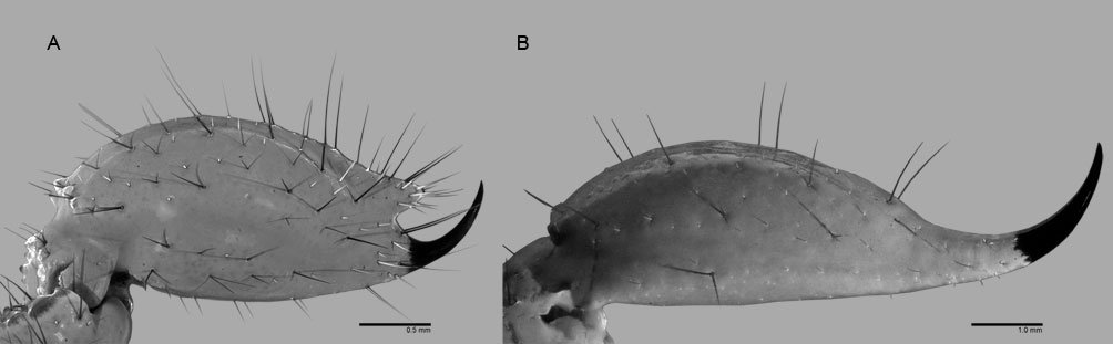
Figure 22. Lateral view of telson of D. zacatecanus (A), and M. spadix (B).
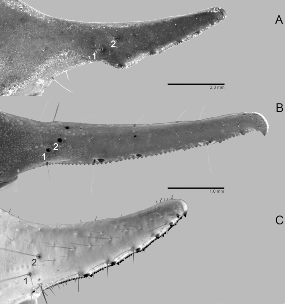
Figure 23. Chela fingers of T. intrepidus (A), V. nigrescens (B), and P. gracilior (C). Trichobothria signaled as follows: 1 basal, 2 = internal terminal.

Figure 24. Carapace of D. zacatecanus (A), P. gracilior (B), and Vaejovis tenamaztlei (C).

Figure 25. Lateral (A), and ventral (B) view of the metasoma of V. nigrescens.

Figure 26. Lateral view of the metasoma of P. gracilior.

Figure 27. Dorsal view of telson of C. glabrimanus (A), P. gracilior (B), and V. tenamaztlei (C).

Figure 28. Dorsal view of pedipalp patella of C. bilineatus (A), and C. glabrimanus (B).

Figure 29. Ventral view of metasoma of C. bilineatus (A, B), and C. glabrimanus (C).
The key provided by Hoffmann (1931) in his original monography distinguishes M. spadix from M. punctatus Karsch based on the body base color and a higher pectinal tooth count, which led him to consider it as a subspecies. However, more recent contributions found further characteristics that differentiate these species. For instance, Fet et al. (2006) presented SEM micrographs of M. punctatus with 2-8 denticles conforming laterobasal aculear serrations (LAS) on the aculeus; however, the specimens of M. spadix examined under UV light during this study do not possess LAS. Finally, M. variegatus is devoid of ventral median carinae in metasomal segment V (Santibáñez-López & Sissom, 2010), which is present in M. spadix (Fig. 32).

Figure 30. Carapace of C. coahuilae (A), and C. glabrimanus (B).

Figure 31. Sternite VII of C. coahuilae (A), and C. glabrimanus (B).

Figure 32. Ventral view of the metasoma of M. spadix.

Figure 33. Ventral view of the metasoma of T. intrepidus.
This contribution is one of the few that present a taxonomic identification key to the species of a political state in Mexico. Currently, only the Mexican states of Baja California, Baja California Sur, Estado de México, and Morelos have a taxonomic key that allows determination to species level (Córdova-Athanasiadis, 2005; González-Santillán, 2004; Williams, 1980).
Natural history collections (NHC) are an invaluable source of information for evolutionary, ecological, taxonomical, and biogeographical research, as well as future applications and yet unexplored fields (Miller et al., 2020). Researchers focused on diverse taxonomical groups such as mammals (McLean et al., 2016), corals (Hoeksema et al., 2011), insects (Kharouba et al., 2019), parasites (Harmon et al., 2019), among others have also stressed the importance of NHC for the evaluation of impacts on biodiversity due to global change and human impact (Shaffer et al., 1998). At the same time, several authors have pointed out a decline in collecting activities and the deposition of specimens due to factors ranging from decline of taxonomical expertise to funding (Rohwer et al., 2022; Salvador & Cunha, 2020; Thompson et al., 2021), increasing regulations and ethical concerns. This contribution epitomizes the importance of local and regional NHCs because without the empirical evidence provided by the CZUAA and the CNAN, this contribution would not be possible, and valuable resources and information, such as a taxonomic key and the recognition of introduced species of public health importance, such as C. balsasensis, would have required comparatively more effort and time to discover.

Figure 34. Ventral view of the telotarsi of V. tenamaztlei (A), and V. aquascalentensis (B).
Acknowledgements
This contribution received funding from the doctoral scholarship 717372 granted to the first author by the Consejo Nacional de Humanidades, Ciencia y Tecnología (Conahcyt) and the project 321671 of Conahcyt and PIB22-2 of the Departamento de Biología de la Universidad Autónoma de Aguascalientes. We thank Fernando Álvarez Padilla of the Laboratorio de Aracnología of the Facultad de Ciencias, UNAM, and José Jesús Sigala Rodríguez of the CZUAA for their help and advice during the photography process of this contribution. We thank Daniel Alexander Carrillo Martínez, Mónica Croce and Patricia García Macías for their assistance during laboratory work. We thank all the collectors, especially Emmanuel González-Martínez, Luis Rodrigo Haro-Tapia, Pablo César Hernández-Romero, Diego Fernando Simijaca-Salcedo, and Iván Villalobos-Juárez, for their constant help. Collection permit FAUT-0213 from Semarnat to JAEM.
Appendix 1. Database of species incidence on a 10 × 10 km grid covering the state of Aguascalientes number of grids (n) = 61. Abbreviations as follows: C. inf = Centruroides infamatus, C. bil = Chihuahuanus bilineatus, C. coa = Chihuahuanus coahuilae, C. gla = Chihuahuanus glabrimanus, D. zac = Diplocentrus zacatecanus, M. spa = Mesomexovis spadix, P. gra = Paruroctonus gracilior, T. int = Thorellius intrepidus, V. agu = Vaejovis aguazarca, V. aqu = Vaejovis aquascalentensis, V. nig = Vaejovis nigrescens, V. ten = Vaejovis tenamaztlei.
| C. inf | D. zac | C. bil | C. coa | C. gla | M. spa | P. gra | T. int | V. agu | V. aqu | V. nig | V. ten |
| 0 | 0 | 0 | 0 | 0 | 0 | 0 | 0 | 0 | 0 | 0 | 0 |
| 1 | 0 | 0 | 0 | 0 | 1 | 0 | 0 | 0 | 0 | 0 | 1 |
| 1 | 0 | 0 | 0 | 1 | 1 | 0 | 1 | 0 | 1 | 0 | 1 |
| 0 | 0 | 0 | 0 | 0 | 0 | 0 | 0 | 0 | 0 | 0 | 0 |
| 0 | 0 | 0 | 0 | 0 | 0 | 0 | 0 | 0 | 0 | 0 | 0 |
| 1 | 0 | 0 | 0 | 0 | 1 | 0 | 0 | 0 | 0 | 0 | 0 |
| 1 | 0 | 0 | 0 | 0 | 1 | 0 | 0 | 0 | 0 | 0 | 0 |
| 1 | 0 | 0 | 0 | 0 | 1 | 0 | 0 | 0 | 1 | 0 | 0 |
| 0 | 0 | 0 | 0 | 0 | 1 | 0 | 0 | 0 | 1 | 0 | 0 |
| 0 | 0 | 0 | 0 | 0 | 0 | 0 | 0 | 0 | 0 | 0 | 1 |
| 0 | 0 | 0 | 0 | 0 | 0 | 0 | 0 | 0 | 0 | 0 | 0 |
| 0 | 0 | 0 | 0 | 0 | 0 | 0 | 0 | 0 | 0 | 0 | 0 |
| 1 | 0 | 0 | 0 | 0 | 0 | 0 | 1 | 0 | 0 | 0 | 0 |
| 1 | 0 | 0 | 0 | 0 | 1 | 0 | 0 | 0 | 0 | 0 | 0 |
| 0 | 0 | 0 | 0 | 0 | 0 | 0 | 0 | 0 | 0 | 0 | 0 |
| 0 | 0 | 0 | 0 | 0 | 0 | 0 | 0 | 0 | 0 | 0 | 0 |
| 0 | 0 | 0 | 0 | 0 | 0 | 0 | 0 | 0 | 0 | 0 | 0 |
| 0 | 0 | 0 | 0 | 0 | 1 | 0 | 0 | 1 | 0 | 0 | 0 |
| 0 | 0 | 0 | 0 | 0 | 0 | 0 | 0 | 0 | 0 | 0 | 0 |
| 0 | 0 | 0 | 0 | 0 | 1 | 0 | 0 | 0 | 0 | 0 | 0 |
| 0 | 0 | 0 | 0 | 0 | 1 | 0 | 0 | 0 | 0 | 0 | 0 |
| 0 | 0 | 0 | 0 | 0 | 0 | 0 | 0 | 0 | 0 | 0 | 0 |
| 0 | 0 | 0 | 0 | 0 | 1 | 0 | 0 | 0 | 0 | 0 | 0 |
| 0 | 0 | 0 | 0 | 0 | 0 | 0 | 0 | 0 | 0 | 0 | 0 |
| 0 | 0 | 0 | 0 | 0 | 0 | 0 | 0 | 0 | 0 | 0 | 0 |
| 0 | 0 | 0 | 0 | 0 | 1 | 0 | 0 | 0 | 0 | 0 | 0 |
| 1 | 0 | 1 | 1 | 1 | 1 | 0 | 0 | 1 | 0 | 1 | 0 |
| 0 | 0 | 0 | 0 | 0 | 1 | 0 | 0 | 0 | 0 | 0 | 0 |
| 0 | 0 | 0 | 0 | 0 | 0 | 0 | 0 | 0 | 0 | 0 | 0 |
| 0 | 0 | 0 | 1 | 0 | 0 | 0 | 0 | 0 | 0 | 0 | 0 |
| 0 | 0 | 0 | 0 | 0 | 0 | 0 | 0 | 0 | 0 | 0 | 0 |
| 0 | 0 | 0 | 0 | 0 | 1 | 0 | 0 | 1 | 0 | 0 | 0 |
| 0 | 0 | 0 | 0 | 0 | 0 | 0 | 0 | 0 | 0 | 0 | 0 |
| 0 | 0 | 1 | 0 | 0 | 1 | 0 | 0 | 1 | 0 | 0 | 0 |
| 0 | 0 | 0 | 1 | 1 | 0 | 0 | 0 | 1 | 0 | 1 | 0 |
| 1 | 0 | 0 | 0 | 0 | 1 | 0 | 0 | 0 | 0 | 0 | 0 |
| 0 | 0 | 0 | 0 | 0 | 0 | 0 | 0 | 0 | 0 | 0 | 0 |
| Appendix 1. Continued | |||||||||||
| C. inf | D. zac | C. bil | C. coa | C. gla | M. spa | P. gra | T. int | V. agu | V. aqu | V. nig | V. ten |
| 0 | 0 | 0 | 0 | 0 | 0 | 0 | 0 | 0 | 0 | 0 | 0 |
| 0 | 0 | 0 | 0 | 0 | 0 | 0 | 0 | 0 | 0 | 0 | 0 |
| 0 | 0 | 0 | 0 | 0 | 0 | 0 | 0 | 0 | 0 | 0 | 0 |
| 0 | 0 | 0 | 0 | 0 | 0 | 0 | 0 | 0 | 0 | 0 | 0 |
| 0 | 0 | 0 | 1 | 1 | 0 | 0 | 0 | 0 | 0 | 1 | 0 |
| 0 | 0 | 0 | 0 | 1 | 0 | 0 | 0 | 0 | 0 | 0 | 0 |
| 1 | 0 | 0 | 1 | 1 | 1 | 0 | 0 | 0 | 0 | 0 | 0 |
| 0 | 1 | 0 | 0 | 0 | 0 | 0 | 0 | 0 | 0 | 0 | 0 |
| 0 | 0 | 1 | 1 | 1 | 0 | 1 | 0 | 0 | 0 | 0 | 0 |
| 0 | 0 | 0 | 0 | 0 | 0 | 0 | 0 | 0 | 0 | 0 | 0 |
| 0 | 0 | 0 | 0 | 0 | 1 | 0 | 0 | 0 | 0 | 0 | 0 |
| 0 | 0 | 0 | 0 | 0 | 0 | 0 | 0 | 0 | 0 | 0 | 0 |
| 0 | 0 | 0 | 0 | 0 | 0 | 0 | 0 | 0 | 0 | 0 | 0 |
| 0 | 0 | 0 | 0 | 0 | 0 | 0 | 0 | 0 | 0 | 0 | 0 |
| 0 | 0 | 0 | 0 | 0 | 0 | 0 | 0 | 0 | 0 | 0 | 0 |
| 0 | 0 | 0 | 0 | 0 | 0 | 0 | 0 | 0 | 0 | 0 | 0 |
| 0 | 0 | 0 | 0 | 0 | 0 | 0 | 0 | 0 | 0 | 0 | 0 |
| 0 | 0 | 0 | 0 | 0 | 0 | 0 | 0 | 0 | 0 | 0 | 0 |
| 0 | 0 | 0 | 0 | 0 | 0 | 0 | 0 | 0 | 0 | 0 | 0 |
| 0 | 0 | 0 | 0 | 0 | 0 | 0 | 0 | 0 | 0 | 1 | 0 |
| 0 | 0 | 0 | 1 | 0 | 0 | 0 | 0 | 0 | 0 | 0 | 0 |
| 0 | 1 | 1 | 0 | 1 | 1 | 0 | 0 | 0 | 0 | 0 | 1 |
| 0 | 0 | 0 | 0 | 0 | 0 | 0 | 0 | 0 | 0 | 0 | 0 |
| 0 | 0 | 0 | 0 | 0 | 0 | 0 | 0 | 0 | 0 | 0 | 0 |
Appendix 2. Database of species incidence in Aguascalientes in 5 years classes, number of classes (n) = 9. Abbreviations as follows: C. inf = Centruroides infamatus, C. bil = Chihuahuanus bilineatus, C. coa = Chihuahuanus coahuilae, C. gla = Chihuahuanus glabrimanus, D. zac = Diplocentrus zacatecanus, M. spa = Mesomexovis spadix, P. gra = Paruroctonus gracilior, T. int = Thorellius intrepidus, V. agu = Vaejovis aguazarca, V. aqu = Vaejovis aquascalentensis, V. nig = Vaejovis nigrescens, V. ten = Vaejovis tenamaztlei.
| C. inf | D. zac | C. bil | C. coa | C. gla | M. spa | P. gra | T. int | V. agu | V. aqu | V. nig | V. ten | |
| 1979-83 | 1 | 1 | 0 | 0 | 1 | 1 | 0 | 0 | 0 | 1 | 0 | 0 |
| 1984-88 | 1 | 0 | 1 | 0 | 1 | 1 | 0 | 0 | 0 | 0 | 1 | 0 |
| 1989-93 | 1 | 1 | 0 | 1 | 1 | 1 | 0 | 0 | 0 | 0 | 0 | 0 |
| 1994-98 | 1 | 0 | 0 | 1 | 1 | 1 | 0 | 0 | 0 | 0 | 1 | 0 |
| 1999-03 | 1 | 0 | 1 | 0 | 1 | 1 | 0 | 1 | 1 | 0 | 0 | 0 |
| 2004-08 | 1 | 1 | 1 | 1 | 1 | 1 | 0 | 0 | 1 | 0 | 1 | 0 |
| 2009-13 | 1 | 1 | 0 | 0 | 1 | 1 | 0 | 0 | 1 | 1 | 1 | 0 |
| 2014-18 | 1 | 1 | 1 | 1 | 1 | 1 | 1 | 1 | 1 | 1 | 1 | 1 |
| 2019-22 | 1 | 1 | 1 | 1 | 1 | 1 | 1 | 1 | 1 | 1 | 1 | 1 |
References
Basualdo, C. V. (2011). Choosing the best non-parametric richness estimator for benthic macroinvertebrates databases. Revista de la Sociedad Entomológica Argentina, 70 , 27–38.
Beck, J., & Kitching, I. J. (2007). Estimating regional species richness of tropical insects from museum data: a comparison of a geography-based and sample-based methods. Journal of Applied Ecology, 44, 672–681. https://doi.org/10.1111/j.
1365-2664.2007.01291.x
Braga-Pereira, G. F., & Santos, A. J. (2021). Asexual reproduction in a sexual population of the Brazilian yellow scorpion (Tityus serrulatus, Buthidae) as evidence of facultative parthenogenesis. Journal of Arachnology, 49, 185–190. https://doi.org/10.1636/JoA-S-20-001
Brown, C. A., Davis, J. M., O’Conell, D. J., & Formanowiz Jr., D. A. (2002). Surface density and nocturnal activity in a west Texas assemblage of scorpions. The Southwestern Naturalist, 47, 409–419. https://doi.org/10.2307/3672498
Bryson, R. W. Jr. (2014) Bacterial endosymbiont infections in ‘living fossils’: a case study of North American vaejovid scorpions. Molecular Ecology Resources, 14, 789–793. https://doi.org/10.1111/1755-0998.12220
Bryson, R. W. Jr., Riddle, B. R., Graham, M. R., Smith, B. T., & Prendini, L. (2013). As Old as the Hills: Montane scorpions in southwestern North America reveal ancient associations between biotic diversification and landscape history. Plos One, 8, e52822. https://doi.org/10.1371/journal.pone.0052822
Chao, A. (1984). Nonparametric estimation of the number of classes in a population. Scandinavian Journal of Statistics, 11, 265–270.
Chávez-Samayoa, F., Díaz-Plascencia, J. E., & González-Santillán, E. (2022). Two new species of Vaejovis (Scorpiones: Vaejovidae) belonging to the mexicanus group from Aguascalientes, Mexico, with comments on the homology and function of the hemispermatophore. Zoologischer Anzeiger, 298, 148–169. https://doi.org/10.1016/j.jcz.2022.04.005
Contreras-Félix, G. A., Francke, O. F., & Bryson Jr., R. W. (2015). A new species of the “mexicanus” group of the genus Vaejovis C. L. Koch, 1836 from the Mexican state of Aguascalientes (Scorpiones: Vaejovidae). Zootaxa, 3936, 131–140. https://doi.org/10.11646/zootaxa.3936.1.8
Contreras-Félix, G. A., & Francke, O. F. (2019). Taxonomic revision of the “mexicanus” group of the genus Vaejovis C. L. Koch, 1836 (Scorpiones: Vaejovidae). Zootaxa, 4596, 1–100. https://doi.org/10.11646/zootaxa.4596.1.1
Córdova-Athanasiadis, M. (2005). Escorpiofauna (Arachnida: Scorpiones) del estado de Morelos, México (Bachelor Thesis). Facultad de Ciencias Biológicas, Universidad Autónoma del Estado de Morelos, Cuernavaca, Morelos.
Degnan, J. H., & Rosenberg, N. A. (2009). Gene tree discordance, phylogenetic inference and the multispecies coalescent. Trends in Ecology & Evolution, 24, 332–340. https://doi.org/10.1016/j.tree.2009.01.009
De la Riva-Hernández, G. (2014). Colección Zoológica de la Universidad Autónoma de Aguascalientes. In J. J. Sigala-Rodríguez, M. D. Barba-Ávila, E. Meza-Rangel, G. Castorena-Esparza, & G. González-Adame (Eds.), La biología en la UAA: 40 años de desarrollo (pp. 77–82). Aguascalientes: Universidad Autónoma de Aguascalientes.
Escoto-Rocha, J., & Delgado-Saldívar, L. (2008). Insectos y arácnidos. InH. Ávila-Villegas, E. D. Melgarejo, & A. Cruz-Angón (Eds.), La biodiversidad en Aguascalientes: estudio de caso (pp. 126–128). Aguascalientes:Comisión Nacional para el Conocimiento y Uso de la Biodiversidad/ Instituto del Medio Ambiente del Estado de Aguascalientes/ Universidad Autónoma de Aguascalientes.
Esposito, L. A., Yamaguti, H. Y., Pinto-Da-Rocha, R., & Prendini, L. (2018). Plucking with the plectrum: phylogeny of the New World buthid scorpion subfamily Centruroidinae Krauss, 1955 (Scorpiones: Buthidae) reveals evolution of three pecten-sternite stridulation organs. Arthropod Systematics & Phylogeny, 76, 87–122. https://doi.org/10.3897/asp.76.e31942
Fattorini, S. (2013). Faunistic knowledge and insect species loss in an urban area: the tenebrionid beetles of Rome. Journal of Insect Conservation, 17, 637–643. https://doi.org/10.1007/s10841-013-9569-5
Fet, V., & Lowe, G. (2000). Family Buthidae C. L. Koch, 1837. In V. Fet, W. D. Sissom, G. Lowe, & M. E. Braunwalder (Eds.), Catalog of the scorpions of the world (1758-1998) (pp. 54–286). New York: New York Entomological Society.
Fet, V., Soleglad, M. E., & Brewer, M. S. (2006). Laterobasal Aculear Serrations (LAS) in scorpion family Vaejovidae (Scorpiones: Chactoidea). Euscorpius, 45, 2–19. https://dx.doi.org/10.18590/euscorpius.2006.vol2006.iss45.1
Fick, S. E., & Hijmans, R. J. (2017). WorldClim 2: new 1km spatial resolution climate surfaces for global land areas. International Journal of Climatology, 37, 4302–4315. https://doi.org/10.1002/joc.5086
Francke, O. F. (2019). Scorpions (Arachnida: Scorpiones) from the Cuatro Ciénegas Basin. In F. Alvarez, & M. Ojeda (Eds.), Animal diversity and biogeography of the Cuatro Ciénegas Basin: an endangered hyperdiverse oasis (pp. 53–59). Switzerland: Springer International Publishing. https://doi.org/10.1007/978-3-030-11262-2_4
Gertsch, W. J., & Soleglad, M. (1966). The Scorpions of the Vejovis boreus Group (Subgenus Paruroctonus) in North America (Scorpionida, Vejovidae). American Museum Noti-
vitates, 2278, 1–54.
González-Santillán, E. (2004). Escorpiofauna del Estado de México (Master Thesis). Instituto de Biología, Universidad Nacional Autónoma de México. México D.F.
González-Santillán, E., & Possani, L. D. (2018). The North American scorpion species of public health importance with a reappraisal of historical epidemiology. Acta Tropica, 187, 264–274. https://doi.org/10.1016/j.actatropica.2018.08.002
González-Santillán, E., & Prendini, L. (2013). Redefinition and Generic revision of the North American Vaejovid scorpion subfamily Syntropinae Kraeplin, 1905, with descriptions of six new genera. Bulletin of the American Museum of Natural History, 382, 1–71. https://doi.org/10.1206/830.1
González-Santillán, E., & Prendini, L. (2015). Phylogeny of the North American vaejovid scorpion subfamily Syntropinae Kraepelin, 1905, based on morphology, mitochondrial
and nuclear DNA. Cladistics, 31, 341–405. https://doi.org/
10.1111/cla.12091
González-Santillán, E., & Prendini, L. (2018). Systematic revision of the North American syntropine vaejovid scorpion genera Balsateres, Kuarapu, and Thorellius, with descriptions of three new species. Bulletin of the American Museum of Natural History, 420, 1–81. https://doi.org/10.1206/0003-0090-420.1.1
Guralnick, R. P., & Van Cleve, J. (2005). Strengths and weaknesses of museum and national survey data sets for predicting regional species richness: Comparative and combined approaches. Diversity and Distributions, 11, 349–359. https://doi.org/10.1111/j.1366-9516.2005.00164.x
Harmon, A., Littlewood, D. T., & Wood, C. L. (2019). Parasites lost: using natural history collections to track disease change across deep time. Frontiers in Ecology and the Environment, 17, 157–166. https://doi.org/10.1002/fee.2017
Hoeksema, B. W., Van der Land, J., Van der Meij, S. E. T., Van Ofwegen, L. P., Reijnen, B. T., Van Soest, R. W. M. et al. (2011). Unforeseen importance of historical collections as baselines to determine biotic change of coral reefs: the Saba Bank case. Marine Ecology, 32, 135–141. https://doi.org/10.1111/j.1439-0485.2011.00434.x
Hoffmann, C. C. (1931). Monografías para la entomología médica de México. Monografía Núm. 2, Los escorpiones de México, Primera Parte: Diplocentridae, Chactidae, Vejovida. Anales del Instituto de Biología, Universidad Nacional Autónoma de México, 2, 291–408.
Hoffmann, C. C. (1932). Monografías para la entomología médica de México Monografía NUM. 2 los escorpiones de México, Segunda Parte: Buthidae. Anales del Instututo de Biología, Universidad Nacional Autónoma de México, 3, 103–361.
Hoffmann, C. C. (1936). La distribución geográfica de los “alacranes peligrosos” en la República Mexicana. Boletín del Instituto de Higiene, 2, 321–330.
INEGI (Instituto Nacional de Estadística y Geografía). 2019. División política estatal 1:250000. Edición 1. Instituto Nacional de Estadística y Geografía. Recovered in September 5th, 2023 from: https://www.inegi.org.mx/app/biblioteca/ficha.html?upc=889463674658
Kharouba, H. M., Lwethwaite, J. M. M., Guralnick, R., Kerr, J. T., & Vellend, M. (2019). Using insect natural history collections to study global change impacts: challenges and opportunities. Philosophical Transactions B., 374, 20170405. http://dx.doi.org/10.1098/rstb.2017.0405
McLean, B. S., Bell, K. C., Dunnnum, J. L., Abrahamson, B., Colella, J. P., Deardorff, E. R. et al. (2016). Natural history collections-based research: progress, promise, and best practices. Journal of Mammalogy, 97, 287–297. https://doi.org/10.1093/jmammal/gyv178
McWest, K. J., Valois, Z. J., & Sissom, W. D. (2017). Scorpions (Arachnida) of the high plains and adjacent canyonlands of northwestern Texas. Texas Journal of Science, 67, 3–38.
Meier, R., & Dikow, T. (2004). Significance of specimen databases from taxonomic revisions for estimating and mapping the global species diversity of invertebrates and repatriating reliable specimen data. Conservation Biology, 18, 478–488.
Miller, S. E., Barrow, L. N., Ehlman, S. M., Goodheart, J. A., Greiman, S. E., Lutz, H. L. et al. (2020). Building Natural History Collections for the Twenty-First Century and beyond. Bioscience, 70, 674–687. https://doi.org/10.1093/biosci/biaa069
Morrone, J. J., Escalante, T., & Rodríguez-Tapia, G. (2017). Mexican biogeographic provinces: Map and shapefiles. Zootaxa, 4277, 277–279. https://doi.org/10.11646/zootaxa.4277.2.8
Oksanen, J., Simpson, G. L., Guillaume-Blancjet, F., Kindt, R., Legendre, P., Minchin, P. R. et al. (2019). ‘Vegan’ Community Ecology Package. R package version 2.6-4. Accessed November 9th, 2022: https://github.com/vegan
devs/vegan
Petersen, F. T., & Meier, R. (2003). Testing species-richness estimation methods on single-sample collection data using the Danish Diptera. Biodiversity and Conservation, 12, 667–686. https://doi.org/10.1023/A:1022495610021
Petersen, F. T., Meier, R., & Larsen, M. N. (2003). Testing species richness estimation methods using museum label data on the Danish Asilidae. Biodiversity and Conservation, 12, 687–701. https://doi.org/10.1023/A:1022464710930
Polis, G. A. (1990). The biology of scorpions. Standford, California: Standford University Press.
Ponce-Saavedra, J., & Francke, O. F. (2004). Una nueva especie de alacrán del género Centruroides Marx (1890) (Scorpiones, Buthidae) de la depresión del Balsas, México. Acta Zoológica Mexicana (nueva serie), 20, 221–232. https://doi.org/10.21829/azm.2004.2022340
Ponce-Saavedra, J., & Francke, O. F. (2013a). Clave para la identificación de especies de alacranes del género Centruroides Marx, 1890 (Scorpiones: Buthidae) en el Centro Occidente de México. Biológicas, 15, 52–62.
Ponce-Saavedra, J., & Francke, O. F. (2013b). Actualización taxonómica sobre alacranes del Centro Occidente de México. Dugesiana, 20, 73–79.
Ponce-Saavedra, J., & Francke, O. F. (2019). Una nueva especie del género Centruroides (Scorpiones: Buthidae) del noroeste de México. Revista Mexicana de Biodiversidad, 90, e902660. https://doi.org/10.22201/ib.20078706e.2019.90.2660
Ponce-Saaveedra, J., Francke, O. F., Cano-Camacho, H., & Hernández-Calderón, E. (2009). Evidencias morfológicas y moleculares que validan como especie a Centruroides tecomanus (Scorpiones, Buthidae). Revista Mexicana de Biodiversidad, 80, 71–84. http://dx.doi.org/10.22201/ib.20078706e.2009.001.585
Ponce-Saavedra, J., Francke, O. F., & Quijano-Ravell, A. F. (2009). Nuevos registros y distribución actualizada de Diplocentrus zacatecanus Hoffmann, 1931 (Scorpiones: Diplocentridae). Entomología Mexicana, 8, 57–60.
Ponce-Saavedra, J., Francke, O. F., Quijano-Ravell, A. F., & Cortés-Santillán, R. (2016). Alacranes (Arachnida: Scorpiones) de importancia para la salud pública en México. Folia Entomológica Mexicana (nueva serie), 2, 45–70.
Ponce-Saavedra, J., Linares-Guillén, J. W., & Quijano-Ravell, A. F. (2022). Una nueva especie de alacrán del género Centruroides Marx (Scorpiones: Buthidae) de la costa Noroeste de México. Acta Zoológica Mexicana (nueva serie), 38, 1–24. https://doi.org/10.21829/azm.2022.3812517
Prendini, L. (2001). Substratum specialization and speciation in southern African scorpions: the effect hypothesis revisited. In V. Fet, & P. A. Selden (Eds.), Scorpions 2001: In Memoriam Gary A. Polis (pp. 113–138). Plymouth, Devon: British Arachnological Society.
Quijano-Ravell, A. F., de Armas, L. F., Francke, O. F., & Ponce-Saavedra, J. (2019). A new species of the genus Centruroides Marx (Scorpiones, Buthidae) from western Michoacán state, México using molecular and morphological evidence. Zookeys, 859, 31–48. https://doi.org/10.3897/zookeys.859.33069
Quijano-Ravell, A. F., & Ponce-Saavedra, J. (2016). A new species of scorpion of the genus Centruroides (Scorpiones: Buthidae) from the state of Michoacán, México. Revista Mexicana de Biodiversidad, 87, 49–61. https://doi.org/10.
1016/j.rmb.2016.01.022
Reyes-Moya, A. G., Mejía-Zúñiga, D., Moncada-Hernández, L. J., Flores-Mendoza, F. J., Saldaña-Alcocer, J. A., González-Acosta, C. et al. (2021). First Report of Centruroides balsasensis in Northern Mexico. Southwestern Entomologist, 46, 275–278. https://doi.org/10.3958/059.046.0129
Rohwer, V. G., Rohwer, Y., & Dillman, C. B. (2022). Declining growth of natural history collections fails future generations. Plos Biology, 20, e3001613. https://doi.org/10.1371/journal.pbio.3001613
Salvador, R. B., & Cunha, C. M. (2020). Natural history collections and the future legacy of ecological research. Oecologia, 192, 641–646. https://doi.org/10.1007/s00442-020-04620-0
Sandoval-Ortega, M. H., Siqueiros-Delgado, M. E., Sosa-Ramírez, J., & Cerros-Tlatilpa, R. (2017). Amaranthaceae (Caryophyllales) richness and distribution in the state of Aguascalientes, Mexico. Botanical Sciences, 95, 203–220. https://doi.org/10.17129/botsci.909
Santibáñez-López, C. E., González-Santillán, E., Monod, L., & Sharma, P. P. (2019). Phylogenomics facilitates stable scorpion systematics: reassessing the relationships of Vaejovidae and a new higher-level classification of Scorpiones (Arachnida). Molecular Phylogenetics and Evolution, 135, 22–30. https://doi.org/10.1016/j.ympev.2019.02.021
Santibáñez-, López, C. E., & Francke, O. F. (2013). Redescription of Diplocentrus zacatecanus (Scorpiones: Diplocentridae) and limitations of the hemispermatophore as a diagnostic trait for genus Diplocentrus. The Journal of Arachnology, 41, 1–10. https://doi.org/10.1636/Ha12-65.1
Santibáñez-López, C. E., Francke, O. F., Ureta, C., & Possani, L. D. (2015). Scorpions from Mexico: from species diversity to venom complexity. Toxins, 8, 2. https://doi.org/10.3390/toxins8010002
Santibáñez-López, C. E., & Sissom, W. D. (2010). A new species of the Vaejovis eusthenura group in Oaxaca, Mexico (Scorpiones: Vaejovidae). Zootaxa, 2493, 49–58. https://doi.org/10.11646/zootaxa.2493.1.4
Shaffer, H. B., Fisher, R. N., & Davidson, C. (1998). The role of natural history collections in documenting species declines. Trends in Ecology & Evolution, 13, 27–30. https://doi.org/10.1016/S0169-5347(97)01177-4
Sigala-Rodríguez, J. J., & Greene, H. W. (2009). Landscape change and conservation priorities: Mexican herpetofaunal perspectives at local and regional scales. Revista Mexicana de Biodiversidad, 80, 231–240. https://doi.org/10.22201/ib.20078706e.2009.001.599
Siqueiros-Delgado, M. E., Rodríguez-Avalos, J. A., Martínez-Ramírez, J., Sierra-Muñoz, J. C., & García-Regalado, G. (2017). Vegetación del estado de Aguascalientes. Aguascalientes: Universidad Autónoma de Aguascalientes.
Sissom, W. D. (1990). Systematics, biogeography and paleontology. In G. A. Polis (Ed.), The biology of scorpions (pp. 31–80). Stanford, CA: Standford University Press.
Sissom, W. D. (2000). Family Vaejovidae. In V. Fet, W. D. Sissom, G. Lowe, & M. E. Braunwalder (Eds.), Catalog of the scorpions of the World (1758-1998) (pp. 503–553). New York: The New York Entomological Society.
Sissom, W. D., & Francke, O. F. (1981). Scorpions of the genus Paruroctonus from New Mexico and Texas (Scorpiones, Vaejovidae). Journal of Arachnology, 9, 93–108.
Sissom, W. D., & Francke, O. F. (1985). Redescription of some poorly known species of the nitidulus group of the genus Vaejovis (Scorpiones, Vaejovidae). Journal of Arachnology, 13, 243–266.
Sissom, W. D., & González-Santillán, E. (2004). A new species and new records for the Vaejovis nitidulus group, with a key to the mexican species (Scorpiones, Vaejovidae). Texas Memorial Museum Speleological Monographs, 6, 1–8.
Sissom, W. D., & Hendrixson, B. E. (2005). A new species of Vaejovis (Scorpiones: Vaejovidae) from Coahuila and Nuevo León, and a key to the vaejovid species from northwestern and north-central Mexico. Zootaxa, 1088, 33–43. https://doi.org/10.11646/zootaxa.1088.1.5
Soberón-Mainero, J., Llorente Bousquets, J., & Oñate, L. (2000). The use of specimen-label databases for conservation purposes: An example using Mexican Papilionid and Pierid butterflies. Biodiversity and Conservation, 9, 1441–1466. https://doi.org/10.1023/A:1008987010383
Soleglad, M. E., & Fet, V. (2008). Contributions to Scorpion Systematics. III. Subfamilies Smeringurinae and Syntropinae (Scorpiones: Vaejovidae). Euscorpius, 71, 1–115. https://dx.doi.org/10.18590/euscorpius.2008.vol2008.iss71.1
Stahnke, H. L. (1971). Some observations of the genus Centruroides Marx (Buthidae, Scorpionida) and C. sculpturatus Ewing. Entomological News, 82, 281–307.
Stockwell, S. A. (1986). The scorpions of Texas (Arachnida, Scorpiones) (Master Thesis). Texas Tech University. Retrieved in: September 5th, 2023 from http://hdl.handle.net/2346/22278
Thompson, C. W., Phelps, K. L., Allard, M. W., Cook, J. A., Dunnum, J. L., Ferguson, A. W. et al. (2021). Preserve a voucher specimen! The critical need for integrating Natural History Collections in infectious disease studies. mBio, 12, e02698. https://doi.org/10.1128/mBio.02698-20
Williams, S. (1968). Scorpions from Northern Mexico: five new species of Vejovis from Coahuila, Mexico. Occasional Papers of the California Academy of Sciences, 68, 1–24.
Williams, S. (1970). A redescription of the scorpion Vejovis bilineatus Pocock (Scorpionida: Vejovidae). The Pan Pacific Entomologist, 46, 238–241.
Williams, S. (1980). Scorpions of Baja California, Mexico and adjacent islands. Occasional Papers of the California Academy of Sciences, 135, 1–127.
Yahia, N., & Sissom, W. D. (1996). Studies on the systematics and distribution of the scorpion Vaejovis bilineatus Pocock (Vaejovidae). The Journal of Arachnology, 24, 81–88.

Luciérnagas de la región golfo-Caribe de México y descripción de 16 especies nuevas
Santiago Zaragoza-Caballero a, Sara López-Pérez b, *, Mireya González-Ramírez a, Geovanni M. Rodríguez-Mirón b, Viridiana Vega-Badillo c, Ishwari G. Gutiérrez-Carranza a, Daniel E. Domínguez-León a, Paulina Cifuentes-Ruiz a, Miriam Aquino-Romero a y Oscar Pérez-Flores d
a Universidad Nacional Autónoma de México, Instituto de Biología, Departamento de Zoología, Apartado postal 70-153, 04510 Ciudad de México, México
b Universidad Nacional Autónoma de México, Facultad de Estudios Superiores Zaragoza, Museo de Zoología, Colección Coleopterológica, Av. Batalla del 5 de mayo s/n, Ejército de Oriente, 09230 Ciudad de México, México
c Instituto de Ecología A.C., Colección Entomológica IEXA “Dr. Miguel Ángel Morón Ríos”, Instituto de Ecología A.C., Carretera Antigua a Coatepec Núm. 351, El Haya, 91073 Xalapa, Veracruz, México
d Universidad Nacional Autónoma de México, Escuela Nacional de Estudios Superiores Unidad Morelia, Laboratorio Nacional de Análisis y Síntesis Ecológica, Antigua Carretera a Pátzcuaro Núm. 8701, 58190 Morelia, Michoacán, México
*Autor para correspondencia: slopez.p@hotmail.com (S. López-Pérez)
Recibido: 11 abril 2024; aceptado: 05 agosto 2024
Resumen
Se presenta información de las luciérnagas presentes en Tamaulipas, Veracruz, Tabasco, Campeche, Yucatán y Quintana Roo, México, región que se denominó golfo-Caribe. Se provee la diagnosis de las especies presentes en esta región y que no se presentan en trabajos previos, así como una clave taxonómica a subfamilia, tribu y género. Se describe una especie nueva del género Magnoculus McDermott y 15 nuevas del género Photinus Laporte, con lo cual el número de especies de luciérnagas en México aumenta a 301. Para las especies nuevas se ilustran los hábitos dorsales y ventrales, así como los genitales de los machos. Para las especies ya descritas y que no se han abordado en trabajos anteriores, se muestran fotografías de los hábitos dorsales y ventrales. Asimismo, se presentan registros nuevos estatales para Photinus anagabrielae Zaragoza-Caballero y Gutiérrez-Carranza y P. hymenodrilus Zaragoza-Caballero y Gutiérrez-Carranza. Adicionalmente, se proponen los siguientes cambios nomenclaturales: Photinus albolimbatus Gemminger, 1870 comb. rest. = P. ivanovitschi Zaragoza-Caballero, Zurita-García y Ramírez-Ponce, 2023, syn. nov.
Palabras clave:Amydetinae; Coleoptera; Lampyridae; Magnoculus; Nuevos registros; Veracruz
© 2024 Universidad Nacional Autónoma de México, Instituto de Biología. Este es un artículo Open Access bajo la licencia CC BY-NC-ND
(http://creativecommons.org/licenses/by-nc-nd/4.0/).
Fireflies of the Gulf-Caribbean region of Mexico and description of 16 new species
Abstract
The fireflies occurring in Tamaulipas, Veracruz, Tabasco, Campeche, Yucatán, and Quintana Roo, Mexico are documented, which is designated Gulf-Caribbean region. The diagnoses of the species that occur in this region, and not presented in previous works, are provided, as well as a taxonomic key for subfamilies, tribes, and genera. A new species of Magnoculus McDermott and 15 new species of Photinus Laporte are described, increasing the number of firefly species in Mexico to 301. The dorsal and ventral views and the male genitalia of the new species are illustrated. For the species already described, but not addressed in previous works, photographs of their dorsal and ventral habitus are shown. New state records for Photinus anagabrielae Zaragoza-Caballero and Gutiérrez-Carranza, and P. hymenodrilus Zaragoza-Caballero and Gutiérrez-Carranza are provided. In addition, the following nomenclatural changes are proposed: Photinus albolimbatus Gemminger, 1870, comb. rest. = P. ivanovitschi Zaragoza-Caballero, Zurita-García y Ramírez-Ponce, 2023, syn. nov.
Keywords: Amydetinae; Coleoptera; Lampyridae; Magnoculus; New records; Veracruz
Introducción
En el mundo se conocen cerca de 2,500 especies de luciérnagas que ocupan una variedad de hábitats y su distribución no es limitada a áreas específicas (Martin et al., 2019; Zaragoza-Caballero et al., 2020). En México se encuentra más de 10% de las luciérnagas y se estima que pueden existir alrededor de 367 especies (Zaragoza-Caballero et al., 2022). En los últimos años se han descrito cerca de 100 especies distribuidas en las zonas centro y norte-occidente del país (Zaragoza-Caballero et al., 2020; Zaragoza-Caballero, López-Pérez et al., 2023), lo cual coloca a México como el segundo país de mayor riqueza de luciérnagas. Las últimas descripciones de nuevas luciérnagas forman parte del proyecto “Luciérnagas de México”, que se lleva a cabo con los objetivos de combatir los déficits linneano y wallaceano, y de contribuir al conocimiento de la taxonomía de estos insectos (Hortal et al., 2015). Durante los últimos estudios realizados, se han descrito mayoritariamente especies del género Photinus Laporte,lo que sugiere a México como su centro de diversificación debido a eventos geológicos y paleoclimáticos, que han ocurrido a lo largo de muchos años (Zaragoza-Caballero et al., 2023).
Los estados del país que colindan con el golfo de México se encuentran entre los más diversos del planeta, pues presentan una variedad de ambientes costeros templados, subtropicales y tropicales (Toledo, 2005). Estos estados son Tamaulipas, Veracruz, Tabasco y Campeche; Yucatán y Quintana Roo también colindan con el golfo, asimismo son parte del mar Caribe. En la zona golfo-Caribe existen pocos trabajos relacionados con las luciérnagas, el trabajo de Zaragoza-Caballero (1995) proporciona información relacionada con las luciérnagas que se encuentran en Los Tuxtlas, Veracruz. Con excepción de este trabajo, no se ha registrado algún otro en la zona golfo-Caribe. En el presente estudio se describen 16 especies nuevas de luciérnagas para los estados mencionados, se ilustran hábitos dorsales y ventrales, así como las distintas vistas de los edeagos. Además, se presenta una clave taxonómica para la separación de géneros.
Materiales y métodos
Este estudio se limita a las especies distribuidas en Tamaulipas, Veracruz, Tabasco, Campeche, Yucatán y Quintana Roo, que forman la región golfo-Caribe (fig. 1). Las nuevas especies se reconocieron a partir del estudio morfológico de 36 ejemplares machos depositados en la Colección Nacional de Insectos (CNIN) del Instituto de Biología, UNAM, igual que el resto de los ejemplares pertenecientes a las especies ya descritas. Todos los ejemplares quedaron depositados en la CNIN.
Para las especies previamente registradas en la región y que no aparecen en la publicación de Zaragoza-Caballero et al. (2020) y Zaragoza-Caballero, López-Pérez et al. (2023), se ilustra el hábito en vista dorsal y ventral, asimismo se muestra un ejemplo de los genitales masculinos para aquellos géneros que se encuentran en la región y que tampoco aparecen en los trabajos antes mencionados. De las especies ya antes registradas en la región: Amydetes fastigiata Illiger, 1807, Aspisoma lepidum (Gorham, 1881), A. yucatanum Olivier, 1908, Bicellonycha facialis (Gorham, 1881), Cratomorphus leoneli Lima et al. 2021, Lucidota diaphanura Gorham, 1881, Phaenolis mexicana McDermott, 1958, Photinoides bidenticauda (McDermott, 1958), Photuris trivittata Lloyd y Ballantyne, 2003, Photinus affinis Gorham, 1880, P. albicauda Gorham, 1881, P. ampliatus Olivier, 1907, P. cordovae Gorham, 1881, P. parvulus Gorham, 1881, Pyractomena striatella Gorham, 1880, P. vexillaria Gorham, 1881 y Vesta thoracica (Olivier, 1790), no se ilustran en fotografías debido a la falta de material; las diagnosis y datos de éstas se recuperaron de las descripciones originales. Para las especies nuevasse ilustra su hábito dorsal y ventral, así como los genitales masculinos. Para la revisión de los ejemplares, la separación del edeago en machos y la toma de medidas se utilizó un microscopio estereoscopio Carl Zeiss™ Discovery V8; las medidas se expresan en mm. Todas las especies de Photinus fueron medidas en el largo y ancho total (LT, AT), largo y ancho del pronoto (LP, AP), largo y ancho de los élitros (LE, AE), largo de las antenas (LA), distancia interocular (DI), distancia interantenal (DIA) y largo y ancho del ojo (LO, AO). Asimismo, se obtuvieron las proporciones largo y ancho de los élitros (LE/AE) y largo de los élitros y largo del pronoto (LE/LP). Los datos anteriores permiten establecer las categorías: chica, corta, mediana, larga y grande en las especies (Zaragoza-Caballero, López-Pérez et al., 2023).

Figura 1. Región golfo-Caribe de México, número de especies previas en la región de acuerdo con Pérez-Hernández et al. (2022).
La información del resumen taxonómico se estandarizó mostrando primero el estado donde se registra la especie, la localidad y posteriormente la fecha; la información restante se presenta de acuerdo con la etiqueta. Para separar información de distintas etiquetas se utilizó “|”. Las fotografías digitales se tomaron en el Laboratorio de Microscopía y Fotografía de la Biodiversidad del Instituto de Biología de la Universidad Nacional Autónoma de México (UNAM), con un microscopio estereoscópico Carl Zeiss™ Axio Zoom V16, equipado con una cámara Zeiss Axiocam MRc5 y con el software ZEN™ = Zeiss Efficient Navigation pro-2012. Las diagnosis de los géneros y especies, así como la distribución, se estructuraron a partir de las descripciones originales y otras fuentes como Gorham (1880a, b, 1881, 1884), Illiger (1807), Laporte (1833), Lima et al. (2021), McDermott (1963, 1964, 1966), Zaragoza-Caballero (1989, 1993, 1995, 1996), Pérez-Hernández et al. (2022), Zaragoza-Caballero et al. (2020), y Zaragoza-Caballero, López-Pérez et al. (2023). Para las distribuciones también se utilizaron ejemplares depositados en la CNIN. Se agrega un asterisco a los géneros y especies que han sido comentados anteriormente en Zaragoza-Caballero et al. (2020) y Zaragoza-Caballero, López-Pérez et al. (2023). El arreglo de los géneros obedece al orden de aparición en la clave para la separación de subfamilias, tribus y géneros, las especies aparecen en orden alfabético. A todos los ejemplares de las especies nuevas se les extrajo el aparato reproductor masculino, siguiendo el protocolo de Gutiérrez-Carranza (2023).
Resultados
Previo a este trabajo, en la región golfo-Caribe de México se tenía el registro de 3 subfamilias, 16 géneros y 90 especies, con esta contribución se adicionan 2 registros estatales nuevos de especies y 16 especies nuevas, por lo que la riqueza de luciérnagas de la región aumentó a 108 (fig. 1, apéndice) y el total de especies mexicanas a 301 (apéndice). El total de las especies presentes en la región representa 30% de las especies de luciérnagas del país. Además, se aportan nuevos registros estatales para Photinus anagabrielae y P. hymenodrilus.
Clave para las subfamilias, tribus y géneros de Lampyridae de la región golfo-Caribe de México
1. Cabeza parcialmente cubierta por el pronoto; clípeo generalmente indistinto, soldado a la frente; sutura frontoclipeal apenas marcada; mandíbulas falcadas 2
1’. Cabeza totalmente cubierta por el pronoto; clípeo bien diferenciado, libre o soldado a la frente; sutura frontoclipeal generalmente membranosa; mandíbulas falcadas o modificadas; con o sin aparato luminoso……………………………………………………………………………………….Lampyrinae 6
2(1). Cabeza horizontal cuando está retraída; mandíbulas sin sedas basales; fositas tentoriales visibles; suturas gulares paralelas o fusionadas; ojos separados; último palpómero labial acuminado; antenas bi o uni-ramosas, con 11 o más antenómeros; pronoto con o sin tubérculos: con o sin aparato luminoso; patas cortas; uñas
simples……………………………………………………………………………………….Amydetinae 3
2’. Cabeza vertical cuando está retraída; mandíbulas con sedas basales; fositas tentoriales no visibles; suturas gulares divergentes; ojos juntos o separados; último palpómero labial generalmente triangular; antenas filiformes, de 11 antenómeros; pronoto sin gibas; con o sin aparato luminoso; patas largas; uñas simples o modifica-
das……………………………………………………………………………………….Photurninae 5
3(2). Antenas largas o cortas con 11 o más antenómeros, uni-ramosas, ramas antenales cortas o largas; ojos grandes o reducidos, separados…………………………………………………………Amydetini 4
3’. Antenas largas con 11 antenómeros, sobrepasando la mitad del cuerpo, ramas antenales cortas y rectas; ojos grandes, no contiguos; mandíbulas largas, fuertemente falcadas; base del pronoto emarginado, ángulos posteriores agudos; segmentos abdominales prominentemente angulados………Vestini Vesta Laporte
4(3). Antenas con 11 antenómeros, ramas antenales largas en abanico; ojos reducidos; pronoto con 2 gibas (tubérculos); órgano luminoso ocupando casi toda el área de los esternitos 6° y 7° Magnoculus McDermott
4’. Antenas con al menos 23 antenómeros; ramas antenales largas en abanico; ojos grandes; pronoto semilunar, sin tubérculos; órgano luminoso ocupando desde 1/2 de longitud y anchura hasta totalidad del área de esternitos 6° y 7° Amydetes Hoffmannsegg
5(2’). Uñas internas y externas bífidas en los machos, simples en las hembras; aparato luminoso presente o ausente, en machos ocupa esternitos 5° y 6°, en hembras la parte media del 5º; edeago con lóbulos laterales casi libres en base dorsal *Bicellonycha Motschulsky
5’. Solo las uñas externas divididas tanto en machos como hembras; aparato luminoso presente, en machos ocupa esternitos 5° y 6° y en hembras el esternito 5°; edeago con lóbulos laterales largos y dorsalmente separados, con 2 largos procesos laterales *Photuris Dejean
6(1). Cuerpo generalmente paralelo; antenas filiformes o serradas y comprimidas; clípeo libre, membranoso; mandíbulas falcadas, expuestas; órganos luminosos generalmente presentes; hembras en ocasiones braquípteras o áp-
teras…………………………………………………………………………………….Photinini 13
6’. Cuerpo generalmente ancho, escutiforme; antenas de forma variada; clípeo indistinto; mandíbulas modificadas, con base cónica, expuestas o no, ápice reducido a dentículo desnudo y agudo; hembras aladas; con o sin aparato luminoso 7
7(6). Tarsos anchos, 4° tarsómero largo, sobrepasando mitad del 5°; hembras con o sin aparato luminoso 9
7’. Tarsos angostos, 4° tarsómero corto, alcanzando casi mitad del 5°; hembras sin aparato luminoso……………………..
…………………………………………………………………………………………..Pleotomini 8
8(7’). Antenas cortas de 13 o 14 antenómeros, del 3-12 ó 13 birrámicas, ramas antenales cortas y lanceoladas; ojos muy grandes; último esternito con borde posterior mucronado *Pleotomus LeConte
8’. Antenas cortas de 11 antenómeros, del 3-10 birrámicas, ramas antenales largas y angostas; ojos reducidos; último esternito dividido en 2 proyecciones apicalmente redondeadas; machos con 2 pequeñas manchas luminosas Phaenolis Gorham
9(7). Cuerpo de forma diversa; ojos grandes cercanos; antenas filiformes, longitud variable; espiráculos abdominales dorsales; hembras con aparato luminoso………………………….Cratomorphini 10
9’. Cuerpo ancho, escutiforme; ojos reducidos distantes; antenas largas, serradas; espiráculos abdominales ventrales; hembras sin aparato luminoso…………………………………………..Lamprocerini *Tenaspis LeConte
10(9). Pronoto sin manchas translúcidas 11
10’. Pronoto con manchas translúcidas; antenas cortas, no rebasando lo largo del pronoto, filiformes; ojos muy grandes, contiguos, ocupando casi toda la cabeza; vertex profundamente excavado *Cratomorphus Motschulsky
11(10). Cuerpo alargado, casi paralelo; pronoto ojival, con o sin quilla longitudinal 12
11’. Cuerpo escutiforme; pronoto trapezoidal; antenas cortas filiformes; ojos grandes, separados; élitros con epipleura ancha, sin costillas; aparato luminoso en machos ocupa toda la superficie de esternitos 5° y 6°, reducido en hembras.. *Aspisoma Laporte
12(11). Pronoto alargado, ojival, paralelo en mitad basal, con quilla longitudinal; aparato luminoso en machos ocupa esternitos 5° y 6°, en hembras reducido *Pyractomena (LeConte)
12’. Pronoto corto, sin quilla; aparato luminoso en machos ocupa esternitos 5° y 6°, en hembras reducidas a par de manchas sobre los mismos segmentos *Aspisomoides Zaragoza-Caballero
13(6). Cuerpo hasta de 12 mm, largo, casi paralelo; ojos grandes o reducidos; pronoto semicircular; élitros con un tipo de pubescencia; con o sin aparato luminoso; edeago sin excrecencias dorso-basales 14
13’. Cuerpo de talla y forma variable, ancho, escutiforme o largo y casi paralelo; ojos de tamaño variable; pronoto semielíptico u ojival; élitros con 2 tipos de pubescencia; con o sin aparato luminoso presente; edeago con o sin excrecencias dorso-basales *Photinus Laporte
14 (13). Aparato luminoso variable, sutura frontoclipeal membranosa o indistinta 15
14’Sin aparato luminoso; clípeo parcialmente visible, sutura frontoclipeal incompleta; 4° metatarsómero bilobulado; esternitos no superpuestos, séptimo del macho tan largo como precedente no mucronado; lóbulo medio del edeago comprimido, cubierto por lóbulos laterales, éstos ventralmente soldados *Pyropyga Motschulsky
15(14). Ojos grandes; sutura frontoclipeal membranosa, clípeo libremente articulado; aparato luminoso presente en machos ocupa esternitos 5° y 6°, y en hembras el 5º; séptimo esternito alargado; lóbulos laterales del edeago soldados basalmente *Photinoides McDermott
15’ Ojos reducidos; sutura frontoclipeal indistinta, clípeo soldado a frente; aparato luminoso reducido o ausente; esternitos foliados, séptimo del macho mucronado; lóbulo medio del aparato reproductor cubierto por lóbulos laterales, éstos con proyección terminal *Lucidota Laporte
Descripciones
Vesta Laporte, 1833
Especie tipo: Vesta chevrolati Laporte, 1833: 133
Blackwelder (1945: 353), Gemminger y Harold (1869: 1638), Gorham (1880a: 13), McDermott (1962: 24, 1964: 37, 1966: 79), Motschulsky (1853: 42), Lacordaire (1857: 316), Okada (1931: 142), Olivier (1885a: 334, 1888: 43, 1907: 16, 1910: 13, 1911: 55), Winkler (1925: 491), Wu (1937: 377).
Macho: cuerpo alargado, subparalelo, sin aparato luminoso; pronoto ojival, con ángulos posteriores prominentes, borde posterior ligeramente emarginado; élitros alargados, con costillas. Cabeza: parcialmente cubierta por pronoto; espacio interocular plano, frente amplia; antenas contiguas, alcanzando mitad de cuerpo, unirramosas, con 11 antenómeros, del 3 al 10 con ramas cortas y anchas, el último lameliforme; ojos ligeramente grandes, enteros, dorsal y ventralmente separados; clípeo soldado a frente, sutura frontoclipeal indistinta; mandíbulas largas, falcadas, dirigidas hacia delante, expuestas; último palpómero maxilar robusto, ovoide; palpómero labial securiforme. Tórax: pronoto ampliamente explanado a los lados; eplipleura angosta; patas medianamente robustas, primer metatarsómero tan largo como 2 siguientes juntos, cuarto mediano, bífido, cubriendo parcialmente al quinto; uñas simples.Abdomen: con 7 esternitos visibles, imbricados, terguitos con ángulos posteriores agudos, pigidio con borde posterior cóncavo; último esternito mucronado, edeago largo, lóbulos laterales soldados dorso-basalmente, casi triangulares, con proyección filiforme, lóbulo medio alargado, rebasando a lóbulos laterales, orificio medio casi terminal. Hembras con último esternito triangular y hendido.
Vesta thoracica (Olivier, 1790)
Lampyris thoracica Olivier, 1790: 81
Cuerpo oscuro; antenas oscuras, comprimidas, un poco más cortas que pronoto; pronoto amarillo, sin manchas; élitros oscuros; edeago similar al de Lucidota, que tiene larga proyección en lóbulos laterales.
Distribución: México: Veracruz. Martin et al. (2019) ubican al género en incertae sedis.
Magnoculus McDermott, 1964
Especie tipo: Megalophthalmus benneti Gray, 1832: 371
Blackwelder (1945: 359), Blackwelder y Arnett (1974: 14), Gorham (1881: 34, 1884: 282), Lacordaire (1857: 335), Laporte (1833: 131, 1840: 265), McDermott (1964: 36), Motschulsky (1853: 49), Olivier (1907: 47, 1911: 53), Zaragoza-Caballero (1995a: 19).
Macho: cuerpo alargado, paralelo; con 1-2 esternitos luminosos; pronoto transverso, con 2 gibas, ángulos posteriores prominentes, borde posterior bisinuado; élitros alargados, con costillas muy evidentes. Cabeza: parcialmente cubierta por pronoto; espacio interocular plano, frente amplia; antenas separadas, cortas, unirramosas, con 11 antenómeros, primero largo, del 3 al 10 casi 2 tercios del primero, con ramas lameladas largas y anchas 6 veces tan largas como antenómero correspondiente; ojos reducidos, enteros, dorsal y ventralmente separados; sutura frontoclipeal indistinta; clípeo transversal; mandíbulas largas, fuertemente curvadas, dirigidas hacia adelante, expuestas; último palpómero maxilar y labial robustos, ojivales. Tórax: pronoto ampliamente explanado a los lados; eplipleura angosta; patas cortas, no comprimidas, primer metatarsómero más o menos semejante a 2 siguientes juntos, cuarto reducido, no cubriendo al quinto; uñas simples.Abdomen: con 7 esternitos visibles, imbricados, ángulos posteriores agudos, pigidio trilobulado; último esternito mucronado; edeago con lóbulos laterales un tanto bifurcados, lóbulo medio curvado y apicalmente ensanchado. Hembras desconocidas.
Magnoculus tlaloque Zaragoza-Caballero y Gutiérrez-Carranza, sp. nov.
Fig. 2A-F
http://zoobank.org:act:917313A8-831C-4BC8-B64B-22A8
E4C34AFF
Macho. Talla: largo 5.6 mm, ancho 2.2 mm. Color castaño oscuro a excepción del ápice de lamelas de antenómeros 3-11, pronoto, escutelo, margen humeral y primer tercio de márgenes laterales de élitros, coxas, trocánteres y fémures amarillos; metepisterno y metasterno castaño ámbar; mandíbulas y uñas ambarinas; esternito 7 blanco cremoso. Sin aparato luminoso, con una mácula lútea en el esternito 6. Cabeza: espacio interocular (0.78 mm) cóncavo, integumento brillante, punteado y espaciadamente piloso; frente oblicua; ojos finamente facetados, reducidos, ovoides, en vista lateral más largos (0.42 mm) que anchos (0.32 mm); distancia interantenal (0.42 mm) 3 veces lo ancho de fosita antenal (0.14 mm); antenas uniflabeladas y largas (2.7 mm), cerca de 3 veces más largas que pronoto (1.05 mm), sobrepasa coxas posteriores, escapo claviforme, casi 2 veces más largo (0.36 mm) que 2 antenitos anteriores juntos (0.2 mm), segundo muy corto (0.04 mm), tercero más largo que siguientes (0.16 mm), cuarto y quinto de 0.12 mm, sexto al décimo de 0.1 mm y undécimo de 1.4 mm, apicalmente ensanchado, tercero a décimo con una lamela apicalmente ensanchada, longitud similar al undécimo antenómero [longitud de las lamelas: 1a = 1.2 mm, 2a = 1.56 mm, 3a-5a = 1.6 mm, 6a = 1.5 mm, 7a = 1.4 mm y 8a = 1.36 mm]; sutura frontoclipeal indistinta; clípeo soldado a la frente con borde distal convexo y cuspidado en medio, superficie glabra escasamente punteada, bordes con sedas largas; labro membranoso, triangular; mandíbulas falcadas, esbeltas, angularmente arqueadas, con sedas en su base externa; palpos maxilares con 4 palpómeros; palpos labiales con 3, palpómeros apicales fusiformes; presenta sutura gular y una fosita tentorial. Tórax: pronoto semicircular, más ancho (1.75 mm) que largo (1.05 mm), borde posterior bisinuado, ángulos posteriores agudos, disco quillado, bituberculado, explanaciones laterales anchas y acanaladas; márgenes con poros glandulares, más abundantes en la región anterior, superficie brillante con pilosidad abundante y decumbente; escutelo espatulado con borde posterior redondeado, superficie plana, brillante, gruesamente punteada y con pilosidad escasa y decumbente; élitros ligeramente aovados, dehiscentes, 4 veces más largos (4.55 mm) que anchos (1.1 mm), presentan 3 costillas, costilla cercana a sutura alcanza ½ de la longitud de los élitros, las 2 externas se extienden y se unen en la parte posterior, integumento rugosamente punteado, brillante y piloso, con pilosidad decumbente, epipleura reducida y gradualmente disminuye al ápice; espiráculos respiratorios mesotorácicos no tubulares, orbiculares, poco esclerosados y con su base proyectada transversalmente; patas cortas y esbeltas, semejantes entre sí pero sucesivamente más largas: longitud de profémures de 1.1 mm y protibias de 1.04 mm, mesofémures de 1.2 mm y mesotibias de 1.1 mm, metafémures de 1.26 mm y metatibias de 1.2 mm, fémures fusiformes, lateralmente aplanados, tibias aplanadas, no acanaladas, rectas, con borde externo crenulado y margen apical redondeado, sin espinas tibiales, tarsómeros lateralmente comprimidos, primer metatarsómero más largo (0.34 mm) que 2 siguientes juntos (0.21 + 0.08 mm), cuarto bífido, uñas simples. Abdomen (fig. 2C): esternitos sin puntuaciones estigmatiformes, de longitud semejante, 1-4 de 0.39 mm, presentan borde posterior ondulado y ángulos posteriores rectos y redondeados, parte media de esternitos 1-3 cóncava y del 4 recta, esternito 5 de 0.3 mm con borde posterior ondulado, parte media recta y ángulos posteriores romos, adicionalmente, presenta un cúmulo de sedas que forman un cono, esternito 6 de 0.3 mm con borde posterior ligeramente ondulado, parte media recta y ángulos posteriores romos, presenta una mácula lútea con superficie glabra, esternito 7 de 0.25 mm con borde posterior ondulado y distintamente acuminado en su parte media, el esternito 8 de 0.25 mm, ojival, con la superficie convexa y el ápice redondo; terguitos 3-6 con proyecciones triangulares agudas en los ángulos posteriores, pigidio trilobulado; edeago (fig. 2D-F): pieza basal simétrica, está presente como una placa dorsal bilobulada, más corta (0.28 mm) que lóbulos laterales (0.32 mm), margen posterior marcadamente hendido; lóbulo medio asimétrico y largo (0.53 mm), cilíndrico con ápice ensanchado, en vista lateral curvado, poco esclerosado, orificio medio abierto ventralmente; lóbulos laterales simétricos (0.32 mm), fusionados ventro-basalmente, en vista lateral triangulares y con ápice romo, superficie interna con un diente. Hembra desconocida.
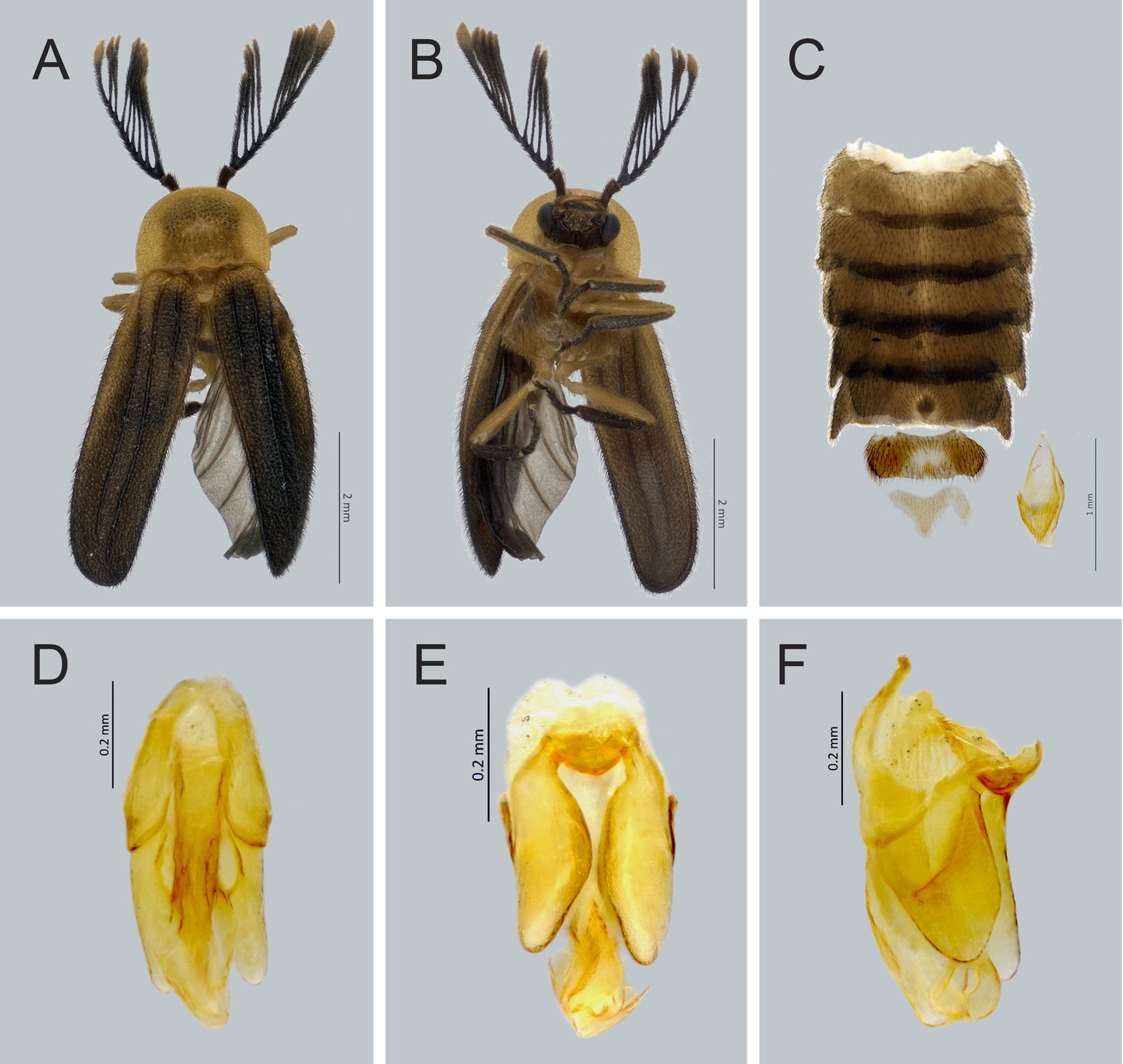
Figura 2. Magnoculus tlaloque Zaragoza-Caballero y Gutiérrez-Carranza, sp. nov. A) Vista dorsal, B) vista ventral, C) abdomen en vista ventral, D) vista dorsal edeago, E) vista ventral edeago, F) vista lateral edeago.
Variación: en algunos ejemplares se registró que solamente la porción apical de la lamela del antenómero 11 es el que presenta la coloración amarilla, mientras que las lamelas de los antenómeros 3-10 son enteramente marrones oscuros, por otra parte, el paratipo proveniente de la localidad de Adolfo Ruiz Cortines en general es de coloración castaño oscuro, con excepción del pronoto.
Resumen taxonómico
Etimología. El nombre específico corresponde a la palabra en náhuatl “tlälòquè”; en la mitología mexica es el nombre con que se refiere a los ayudantes de la deidad “Tláloc”, encargados de repartir la lluvia. Género neutro. En reconocimiento a la narrativa tradicional de algunos sitios de avistamiento de luciérnagas en donde se asocia la presencia de “tlaloques” con la temporada de lluvias y, por tanto, el surgimiento de estos insectos luminosos.
Tabla 1
Características de Magnoculus guatemalae y M. tlaloque, sp. nov.
| Carácter | M. guatemalae | M. tlaloque |
| Talla | largo: ≥ 8 mm, ancho: ≥ 3 mm | largo: 5.6 mm, ancho: 2.2 mm |
| Ojos | grandes: 2/3 de la cabeza | reducidos: 2/5 de la cabeza |
| Ápice de las lamelas de los antenómeros 3-11 | negro | amarillo |
| Color del pronoto | amarillo, con máculas rojizas | amarillo, sin máculas rojizas |
| Color de los élitros | margen humeral y lateral: castaño oscuro | margen humeral y lateral: amarillo |
| Trocánteres, fémures y tibias | ferruginosos | amarillos |
| Mácula lútea | en el borde posterior del esternito 4 | en la superficie media del esternito 6 |
Material examinado. Holotipo. Macho: México, Veracruz, E.B.T., 18°21’03.0’’ N, 95°02’38’’ O, 24-VII-2013 al 16-VIII-2013, 128 m snm, Jardín Botánico Acahual de B.T.P., C5 Malaise 11, Col. M. Madora | COL.TIP-03938. Paratipos: 6 machos. Uno con los mismos datos que el holotipo; 1, Estación de Biología “Los Tuxtlas”, 12-VIII-1985, 160 m snm, Col. A. Ibarra; 1, misma localidad, 15-VIII-1986, 180 m snm, Col. A. Ibarra; 1, El Vigía, 01-VIII-1986, 480 m snm, T.M., Col. E. Ramírez; 1, 17-IX-1989, Col. E. Barrera; 1, Adolfo Ruiz Cortines, 07-VI-2018, Cols. P.C.R., V.V.B. y S.L.P. | COL.TIP-03939-03944.
Comentarios taxonómicos
Zaragoza-Caballero (1995) ubicó a esta especie como cercana a M. guatemalae; sin embargo, este especimen se comparó con fotos del ejemplar tipo depositado en el Museo de Historia Natural de Londres y se reconocieron características que permiten segregarla de M. guatemalae (tabla 1).
Amydetes Illiger, 1807
Especie tipo: Amydetes fastigiata Illiger, 1807: 342
Blackwelder (1945: 360), Gemminger y Harold (1869: 1649), Gorham (1880b: 97, 1881: 62), Jeng (2008), Kuntzen (1912: 86), Lacordaire (1857: 334), Laporte (1833: 127), McDermott (1964: 36, 1966: 77), Motschulsky (1853: 49), Olivier (1899: 73, 1907: 48, 1911: 57), Silveira y Mermudes (2014: 201-248), Viviani (2001: 129, 2010: 107, 2012:29), Westwood (1830: 62).
Cuerpo alargado, pequeño, paralelo; con 2 esternitos luminosos; pronoto transverso, borde posterior bisinuoso, ángulos posteriores agudos; élitros alargados, submembranosos, con costillas evidentes. Cabeza: parcialmente cubierta por pronoto; espacio interocular plano, frente amplia; antenas contiguas, medianas, con 20 o más antenómeros, a partir del tercero con ramas largas en abanico, último similar a ramas; ojos muy grandes, enteros, dorsal y ventralmente separados; sutura frontoclipeal indistinta; mandíbulas dirigidas hacia delante, expuestas; último palpómero maxilar y labial robustos, ovalados. Tórax: pronoto ampliamente explanado lateralmente; eplipleura angosta; patas delgadas, primer tarsómero más largo que 2 siguientes juntos, cuarto reducido, quinto en gran parte libre, uñas simples.Abdomen: no lobulado, ángulos posteriores romos; pigidio trilobulado; último esternito truncado o ligeramente escotado. Hembra desconocida.
Amydetes fastigiata Illiger, 1807
Cuerpo alargado, negro; pronoto blanquecino, disco con una mancha negra y 2 pequeñas manchas oblicuas anaranjadas; élitros oscuros, posteriormente ensanchados, con margen lateral y sutural blanquecino; parte media de esternitos 5-6 con manchas luminosas; edeago con pieza basal reducida, lóbulos laterales cortos, lóbulo medio largo y cilíndrico.
Para Silveira y Mermudes (2014), A. plumicornis Latreille, 1811, es sinónimo de A. fastigiata Illiger, 1807.
Distribución: México: Yucatán.
*Bicellonycha Motschulsky,1853
Especie tipo: Bicellonycha albilatera Gyllenhal, 1817: 21
Blackwelder (1945: 361), Blackwelder y Arnett (1974: 13), Cicero (1982: 270), Gorham (1881: 56), Lacordaire (1857: 335), McDermott (1964: 41, 1966: 93), Motschusky (1853: 54), Olivier (1907: 57, 1909: 113, 1911: 107), Zaragoza-Caballero (1995a: 62), Zaragoza-Caballero et al. (2020, 2023). Diagnosis en Zaragoza et al. (2020, 2023).
Bicellonycha albomarginata Zaragoza-Caballero, 1989
Fig. 3A
Macho. Talla: largo 10.2 mm; ancho 2.96 mm. Cuerpo ovoide, pronoto negro con margen amarillo y élitros negros con margen amarillo y una tenue banda oblicua amarilla; ojos grandes; clípeo unidentado; aparato luminoso presente en los esternitos 5-6 más largos que precedentes, con puntuaciones laterales, borde posterior del 7 mucronado; edeago corto, lóbulos laterales paralelos, cubriendo dorsalmente al lóbulo medio provisto de 2 dientes dorsolaterales.
Distribución: México: Oaxaca, Veracruz.
*Bicellonycha amoena (Gorham, 1880b). En Zaragoza-Caballero et al. (2020).
Photuris amoena Gorham, 1880b: 108
Distribución: Chiapas, Colima, Guerrero, Hidalgo, Jalisco, Estado de México, Guanajuato, Morelos, Michoacán, Nayarit, Oaxaca, Puebla, San Luis Potosí, Tamaulipas y Veracruz.
*Bicellonycha collaris (Gorham, 1880b). En Zaragoza-Caballero et al. (2020).
Photuris collaris Gorham, 1880:107
Distribución: Chiapas, Estado de México, Morelos, Puebla y Veracruz.
Bicellonycha crassa (Gorham, 1884)
Photuris crassa Gorham, 1884: 274
Figs. 3B, 4A
Macho. Talla: largo 9.17 mm, ancho 3.33 mm. Cuerpo casi paralelo, pronoto amarillo, con una mancha negra alargada; élitros amarillos con una banda longitudinal ancha que va desde escutelo a parte media uniéndose con una mancha negra; ojos medianos; clípeo con 3 dientes; aparato luminoso presente en esternitos 5-6, éstos tan largos como precedentes, sin puntuaciones laterales; borde posterior del 7 mucronado con ápice redondeado; edeago corto, lóbulos laterales anchos y espatulados, lóbulo medio con una quilla triangular.
Distribución: México: Chiapas, Oaxaca y Veracruz.
*Bicellonycha discicollis (Gorham, 1881). En Zaragoza-Caballero et al. (2020).
Photuris discicollis Gorham, 1881: 57.
Distribución: Chiapas, Hidalgo, Estado de México, Morelos, Nayarit, Oaxaca y Veracruz.
Bicellonycha facialis (Gorham, 1881)
Photuris facialis Gorham, 1881: 59
Macho. Talla: largo 7.99 mm; ancho 2.99 mm. Cuerpo paralelo, castaño, pronoto con una pequeña mancha negra basal; élitros rojizos, marginados; ojos pequeños, ovoides; clípeo con 3 dientes; aparato luminoso presente en esternitos 5-6, éstos tan largos como precedentes, sin puntuaciones laterales; esternito 7 con un mucrón largo y apicalmente agudo; edeago corto, cilíndrico, lóbulos laterales anchos y espatulados, lóbulo medio con 3 dientes dorsales.
Distribución: Veracruz.
*Bicellonycha gorhami Zaragoza-Caballero, 1989. En Zaragoza-Caballero et al. (2020).
Distribución: Estado de México, Guerrero, Jalisco, Morelos y Veracruz.
*Bicellonycha limbata Pic, 1924. En Zaragoza-Caballero et al. (2020).
Distribución: Chiapas, Jalisco, Morelos, Oaxaca, Puebla y Veracruz.
*Bicellonycha mexicana (Gorham, 1880b). En Zaragoza-Caballero et al. (2020).
Photuris mexicana Gorham, 1880: 108
Distribución: Estado de México, Morelos, Puebla y Veracruz.
*Bicellonycha ruficollis (Gorham, 1880b). En Zaragoza-Caballero et al. (2020).
Photuris ruficolli Gorham, 1880: 107
Distribución: Estado de México, Hidalgo, Morelos y Veracruz.
*Bicellonycha stigmatica (Olivier, 1886). En Zaragoza-Caballero et al. (2020).
Photuris stigmatica Olivier, 1886: 245
Distribución: Chiapas, Oaxaca, Puebla y Veracruz.
*Photuris Dejean, 1833
Especie tipo: Lampyris versicolor Fabricius, 1798: 125 designado por Barber, 1951:11
Blackwelder (1945: 360), Blackwelder y Arnett (1974: 12), Buck (1951: 14), Dejean (1833: 103), Fabricius (1798: 125), Gorham (1880b: 105, 1881: 59), Lacordaire (1857: 339), Laporte (1833: 144), LeConte (1852: 337, 1881: 37), McDermott (1964: 40, 1966: 88), Motschulsky (1852: 38), Olivier (1886: 201, 1907: 57, 1909: 113, 1911: 106), Zaragoza-Caballero (1995a: 55). Diagnosis en Zaragoza-Caballero et al. (2020, 2023).
*Photuris fulvipes (Blanchard, 1846). En Zaragoza-Caballero et al. (2020).
Lampyris fulvipes Blanchard, 1846: 115
Distribución: Estado de México, Hidalgo, Morelos y Veracruz.
*Photuris lugubris Gorham, 1881. En Zaragoza-Caballero et al. (2020, 2023).
Distribución: Ciudad de México, Guerrero, Jalisco, Morelos, Oaxaca y Tamaulipas.
Photuris mollis Gorham, 1880
Figs. 3C, 4B
Macho. Talla: largo 7.00-8.00 mm, ancho 1.71 mm. Cuerpo alargado, paralelo, castaño, pronoto blanquecino con una pequeña mancha negra piriforme; ojos grandes, reniformes; clípeo transverso; élitros marrones, márgenes sutural y laterales amarillos; aparato luminoso ocupando esternitos 5-6; edeago transparente, con pieza basal muy corta, lóbulos laterales largos con proyección lateral aún más larga, lóbulo medio largo y apicalmente
comprimido.
Distribución: México: Oaxaca y Veracruz.
*Photuris tenuisignathus Zaragoza-Caballero, 1995. En Zaragoza-Caballero et al. (2023).
Distribución: Chiapas, Oaxaca, San Luis Potosí y Veracruz.
Photuris trivittata Lloyd y Ballantyne, 2003
Figs. 3D, 4C
Macho. Talla: largo 14 mm; ancho 6 mm. Cuerpo ovoide, amarillo, pronoto con una mancha negra longitudinalmente dividida; élitros amarillos con 3 o 4 bandas oscuras; ojos grandes, reniformes; clípeo pentagonal; aparato luminoso presente en esternitos 5-6, éstos, más largos que precedentes; esternito 7 con un mucrón mediano y romo; edeago con pieza basal muy corta, lóbulos laterales largos con una proyección lateral aún más larga, lóbulo medio largo y comprimido.
Distribución: México: Chiapas, Quintana Roo, Tabasco y Veracruz.
*Photuris versicolor (Fabricius, 1798)
Lampyris versicolor Fabricius, 1798: 125
Photuris quadrifulgens Barber, 1951
Especie citada por Zaragoza-Caballero (1995a) y Zaragoza-Caballero et al. (2020) como P. trilineata (Say, 1835).
Distribución: Puebla, Oaxaca y Veracruz.
*Pleotomus LeConte, 1861
Especie tipo: Pleotomus pallens LeConte, 1866: 88
Blackwelder y Arnett (1974: 1), Gorham (1880a: 10), Green (1948: 69, 1959: 91), LeConte (1861: 184, 1881: 38), McDermott (1964: 20; 1966: 20), Olivier (1907: 10, 1911: 42), Zaragoza-Caballero (2002: 325), Zaragoza-Caballero et al. (2020: 56) y Zaragoza-Caballero, López-Pérez et al. (2023: 8). Diagnosis en Zaragoza et al. (2020) y Zaragoza-Caballero, López-Pérez et al. (2023).
*Pleotomus pallens LeConte, 1866. En Zaragoza et al. (2020) y Zaragoza-Caballero, López-Pérez et al. (2023).
Distribución: Durango, Jalisco, Michoacán, Nayarit, Nuevo León, Oaxaca, Puebla, San Luis Potosí, Sinaloa, Tamaulipas y Veracruz.
*Phaenolis Gorham, 1880
Especie tipo: Phaenolis laciniatus Gorham, 1880a: 10
Blackwelder (1945: 351), Blackwelder y Arnett (1974: 14), Gorham (1880a: 10, 1881: 31); Olivier (1885b: 142, 1907: 10; 1911: 46), McDermott (1958: 22, 1964: 26, 1966: 78), Zaragoza-Caballero (1995: 20). Diagnosis en Zaragoza-Caballero et al. (2020).
*Phaenolis alboterminatus Zaragoza-Caballero, 1995. En Zaragoza-Caballero et al. (2020)
Distribución: Morelos y Veracruz.
Phaenolis mexicana McDermott, 1958
Macho. Talla: largo 12.6 mm, ancho 4.75mm. Cuerpo ovoide, color negro, pronoto totalmente amarillo con una mancha cuadrangular castaño; élitros negros, con 3 costillas; sin aparato luminoso; esternitos 5-6, marrones, sin puntuaciones laterales; esternito 7 corto, emarginado y amarillento; esternito 8 bilobulado y amarillento; pieza basal del edeago asimétrica, lóbulos laterales asimétricos, dorsalmente soldados, más cortos que lóbulo medio, éste, claramente curvado.
Distribución: México: Puebla y Veracruz.
Phaenolis ustulata Gorham, 1880
Figs. 3E, 4D
Macho. Talla: largo 11.18-16.14 mm; ancho 5.45-5.73 mm. Cuerpo ovoide, pronoto amarillento, con una mancha negra variable; élitros con mitad anterior amarillenta y apical negra; sin aparato luminoso; esternitos 5-6, tan largos como precedentes, sin puntuaciones laterales, borde posterior del 7 bicóncavo, borde posterior del 8 ojival; pieza basal del edeago asimétrica, lóbulos laterales asimétricos, dorsalmente soldados, más cortos que lóbulo medio, éste, claramente curvado.
Distribución: México: Chiapas, Oaxaca y Veracruz.
*Tenaspis LeConte, 1881
Especie tipo: Hyas angularis Gorham, 1880a: 7
Blackwelder (1945: 355), Blackwelder y Arnett (1974: 1), Gorham (1884: 250), Green (1948: 68, 1959: 93), LeConte (1881: 33), McDermott (1964: 23, 1966: 26), Olivier (1885b: 135, 1907: 22, 1911: 67); Zaragoza-Caballero (1995: 23), Zaragoza-Caballero, López-Pérez et al. (2023: 9). Diagnosis en Zaragoza-Caballero, López-Pérez et al. (2023).
Tenaspis gonzalenzis Zaragoza-Caballero, 1995
Figs. 3F, 4E
Macho. Talla: largo 11.32 mm, ancho 6 mm. Cuerpo escudiforme, color negro, pronoto amarillo rojizo, con 3 manchas negras, élitros negros, sin aparato luminoso; esternitos 5-6, más largos que precedentes, sin puntuaciones laterales, borde posterior del 7 cóncavo, 8 profundamente emarginado, ángulos posteriores de terguitos muy prominentes; pieza basal del edeago simétrica, tan larga como lóbulos laterales, éstos, en vista lateral casi cuadrangulares, con una proyección curvada, lóbulo medio membranoso, más largo que lóbulos laterales.
Distribución: México: Chiapas y Veracruz.
*Cratomorphus Motschulsky, 1853
Especie tipo: Photinus fabricii Laporte, 1840: 258; designación original.
Blackwelder (1945: 355), Blackwelder y Arnett (1974: 11), Gorham (1880a: 33), Green (1948: 68, 1959: 93), McDermott (1964: 23, 1966: 27), Motschulsky (1853: 35), Lacordaire (1857: 325), Olivier (1895: 145, 1907: 28, 1911: 75), Zaragoza-Caballero (1995: 26, 1996: 320), Zaragoza-Caballero, López-Pérez et al. (2023: 11). Diagnosis en Zaragoza-Caballero, López-Pérez et al. (2023).
*Cratomorphus concolor (Perty, 1830). En Zaragoza-Caballero et al. (2020) y Zaragoza-Caballero, López-Pérez et al. (2023).
Lampyris concolor Perty, 1830: 30
Distribución: Campeche, Chiapas, Estado de México, Hidalgo, Puebla, Quintana Roo, San Luis Potosí, Tabasco, Veracruz y Yucatán.
Cratomorphus leoneli Lima et al., 2021. Ver fotografías en Lima et al. (2021)
Macho. Talla: largo 11.7 mm; ancho 2.4 mm. Cuerpo escudiforme, color amarillo obscuro, pronoto castaño, márgenes amarillos, manchas translúcidas reniformes; élitros amarillo oscuro, con 2 costillas longitudinales, aparato luminoso ocupando parte de esternitos 5-6, éstos tan largos como precedentes, sin puntuaciones laterales, borde posterior del 7 cóncavo, con 2 puntos blanquecinos, 8 semicircular; pieza basal del edeago asimétrica, lóbulos laterales dorso basalmente soldados, éstos, en vista lateral casi triangulares, lóbulo medio lateralmente comprimido, curvado, ápice redondeado.
Distribución: México: Campeche, Chiapas, Oaxaca.
Cratomorphus picipennis Gorham, 1881
Figs. 3G, 4F
Macho. Talla: largo 13.05-16.25 mm, ancho 6.11-7.92 mm. Cuerpo escudiforme, pronoto amarillento, con una mancha piriforme negra, élitros negros, con margen sutural y lateral amarillo y 2 costillas longitudinales, aparato luminoso ocupando parte de esternitos 5-6, éstos, tan largos como precedentes, sin puntuaciones laterales, borde posterior del 7 cóncavo, 8 semicircular; pieza basal del edeago simétrica, lóbulos laterales dorso-basalmente soldados, éstos, en vista lateral casi triangulares, lóbulo medio lateralmente comprimido, cubierto por los lóbulos laterales.
Distribución: México: Chiapas y Veracruz.
*Cratomorphus signativentris Olivier, 1895. En Zaragoza-Caballero, López-Pérez et al. (2023).
Distribución: Campeche, Chiapas, Oaxaca, Querétaro, Quintana Roo, San Luis Potosí, Tabasco y Veracruz.
*Aspisoma Laporte, 1833
Especie tipo: Lampyris ignita Linnaeus, 1767: 645; designada por McDermott, 1966: 229.
Blackwelder (1945: 356), Blackwelder y Arnett (1974: 2), Gorham (1881: 53), Green (1948: 68, 1959: 93), Lacordaire (1857: 326), Laporte (1833: 145), Linnaeus (1767: 645), McDermott (1964: 24, 1966: 229), Motschulsky (1853: 35), Olivier (1907: 29, 1911: 78), Zaragoza-Caballero (1995: 28), Zaragoza-Caballero et al. (2020: 5) y Zaragoza-Caballero, López-Pérez et al. (2023: 9). Diagnosis en Zaragoza-Caballero et al. (2020) y Zaragoza-Caballero, López-Pérez et al. (2023).
*Aspisoma aegrota (Gorham, 1880b). En Zaragoza-Caballero et al. (2020).
Aspidosoma aegrota Gorham, 1880b: 84
Distribución: Chiapas, Hidalgo, Jalisco, Morelos, Michoacán, Oaxaca, Puebla, San Luis Potosí y Veracruz.
*Aspisoma depictum (Gorham, 1880b). En Zaragoza-Caballero, López-Pérez et al. (2023).
Aspidosoma depictum Gorham 1880b: 85
Distribución: Campeche, Michoacán y Veracruz.
*Aspisoma diaphana (Gorham, 1880). En Zaragoza-Caballero et al. (2020).
Aspidosoma diaphana Gorham, 1880b: 86
Distribución: Oaxaca, Puebla y Veracruz.
*Aspisoma ignitum (Linnaeus, 1767). En Zaragoza-Caballero et al. (2020).
Lampyris ignita Linnaeus, 1767: 645
Distribución: Campeche, Morelos, Puebla, San Luis Potosí y Veracruz.
Aspisoma lepidum (Gorham, 1881)
Aspidosoma lepidum Gorham, 1881: 54
Macho. Talla: largo 7-8 mm. Cuerpo ovalado, brillante, pronoto amarillo, manchas laterales fusionadas con mancha discal, sin alcanzar margen posterior, élitros oscuros con bandas pálidas, estrechamente punteados aparato luminoso del macho ocupa esternitos 5 y 6, en hembra ocupa parte media del 5.
Distribución: México: Campeche.
*Aspisoma pulchellum (Gorham, 1880b). En Zaragoza-Caballero et al. (2020).
Aspidosoma pulchellum Gorham, 1880b: 86
Distribución: Chiapas, Estado de México, Tabasco y Veracruz.
Aspisoma quasidiaphana Zaragoza-Caballero, 1995
Figs. 3H, 4G
Macho. Talla: largo 12.6 mm, ancho 6.91 mm. Cuerpo escudiforme, color amarillo; mancha negra del pronoto irregular, más amplia en base; élitros amarillos, con 4 bandas longitudinales y 2 transversas marginales de color negro, centro de los esternitos 5-6 con aparato luminoso; éstos más largos que precedentes, con puntuaciones laterales, borde posterior del 7 casi recto, 8 ojival; pieza basal del edeago simétrica, lóbulos laterales dorso basalmente soldados, lóbulo medio lateralmente comprimido, cubierto por lóbulos laterales.
Distribución: México: Veracruz.

Figura 3. Vista dorsal de especies de Lampyridae. A) Bicellonycha albomarginata, B) Bicellonycha crassa, C) Photuris mollis, D) P. trivittata, E) Phaenolis ustulata, F) Tenaspis gonzalenzis, G) Cratomorphus picipennis, H) Aspisoma quasidiaphana.
Aspisoma yucatanum Olivier, 1908
Macho. Talla: largo 7-8 mm. Cuerpo escudiforme, ambarino, pronoto amarillo, con una mancha triangular oscura y 2 puntos laterales de color castaño; escutelo castaño; élitros marrones, con margen lateral y sutural amarillo.
Distribución: México: Yucatán.
*Pyractomena Melsheimer, 1846
Especie tipo: Pyractomena lucifera Melsheimer, 1846; designada por McDermott, 1966.
Blackwelder (1945: 355), Blackwelder y Arnett (1976: 2), Gorham (1880a: 32), Green (1948: 68, 1957: 237, 1959: 93), Lacordaire (1857: 324), LeConte (1851: 336), Leng y Mutchler (1922: 452), McDermott (1964: 25, 1966: 32), Melsheimer (1846: 304), Motschulsky (1853: 37), Olivier (1899: 371, 1907: 31, 1911: 99), Zaragoza-Caballero et al. (2020: 7) y Zaragoza-Caballero, López-Pérez et al. (2023: 10). Diagnosis en Zaragoza-Caballero et al. (2020) y Zaragoza-Caballero, López-Pérez et al. (2023).
*Pyractomena angulata (Say, 1825). En Zaragoza-Caballero et al. (2020) y Zaragoza-Caballero, López-Pérez et al. (2023).
Lampyris angulata Say 1825: 261
Distribución: Morelos, Nuevo León, Puebla, San Luis Potosí, Tamaulipas y Veracruz.
Pyractomena striatella Gorham, 1880
Macho. Talla: largo 10-13 mm. Cuerpo alargado, castaño, ovoide, pronoto ojival, carinado, amarillo, con 2 manchas oscuras laterales y una apical; élitros marrones, con margen lateral y sutural amarillo y bicarinado; esternitos oscuros con margen posterior amarillo y lateral rojizo, esternitos 5-6 con aparato luminoso, éstos más largos que los precedentes, sin puntuaciones laterales, borde posterior del 7 casi recto, 8 mucronado.
Distribución: México: Chiapas, Quintana Roo y Tabasco.

Figura 4. Vista ventral de especies de Lampyridae. A) Bicellonycha crassa, B) Photuris mollis, C) P. trivittata, D) Phaenolis ustulata, E) Tenaspis gonzalenzis, F) Cratomorphus picipennis, G) Aspisoma quasidiaphana.
Pyractomena vexillaria Gorham, 1881
Macho. Talla: largo 15 mm. Cuerpo alargado, castaño, ovoide; antenas más cortas que pronoto, carinado, anaranjado y con 2 manchas angostas oscuras centro-basales; élitros bicarinados, acuminados, marrones, con margen lateral y sutural amarillo; esternitos amarillos, a excepción del cuarto.
Distribución: México: Tabasco y Veracruz.
*Aspisomoides Zaragoza-Caballero, 1995
Especie tipo: Aspidosoma bilineatum Gorham, 1880b, Zaragoza-Caballero, 1995 designación original. Diagnosis en Zaragoza-Caballero et al. (2020) y Zaragoza-Caballero, López-Pérez et al. (2023).
*Aspisomoides bilineatum (Gorham, 1880). En Zaragoza-Caballero et al. (2020).
Aspidosoma bilineatum Gorham, 1880b: 86
Distribución: Guerrero, Jalisco, Morelos, Michoacán, Nayarit, Oaxaca, San Luis Potosí, Sinaloa, Sonora, Tabasco, Tamaulipas y Veracruz.
*Aspisomoides costatum (Gorham, 1880). En Zaragoza-Caballero, López-Pérez et al. (2023).
Aspidosoma costatum Gorham, 1880b: 87
Distribución: Chiapas, Durango, Guerrero, Oaxaca, Tabasco y Veracruz.
*Photinus Laporte, 1833
Ellipolampis Motschulsky, 1853
Ellychnia Blanchard, 1845
Ellychnia Dejean, 1833
Ellychnia LeConte, 1881
Ellychnia Motschulsky, 1853
Lamprodes Motschulsky, 1853
Macrolampis Motschulsky, 1853
Paraphotinus Zaragoza-Caballero, 1995
Especie tipo: Lampyris pallens Fabricius, 1798: 96; designada por Fleutiaux et al. (1947).
Barber (1941: 2), Blackwelder (1945: 357), Blackwelder y Arnett (1974: 6), Fall (1927: 208), Gorham (1880a: 22, 1881: 38, 1884: 238); Green (1948: 68, 1956: 561, 1959: 93), Lacordaire (1857: 321), LeConte (1852: 334, 1881:34), Leng y Mutchler (1933: 21), McDermott (1964: 26, 1966: 35), Motschulsky (1853: 40), Olivier (1907: 33), Zaragoza-Caballero (1995a: 36), Zaragoza-Caballero et al. (2020: 10), Zaragoza-Caballero, López-Pérez et al. (2023: 13) y Zaragoza-Caballero, Zurita-García et al. (2023: 267). Diagnosis en Zaragoza-Caballero et al. (2020) y Zaragoza-Caballero, López-Pérez et al. (2023).
Photinus acremophallus Zaragoza-Caballero y Gutiérrez-Carranza, 2018
Photinus (Paraphotinus) acremophallus Zaragoza-Caballero y Gutiérrez-Carranza, 2018: 161
Figs. 5A, 6A, 7A, 8A, 9A
Macho. Talla: largo 6.19 mm, ancho 1.78 mm. Cuerpo ovoide, color castaño, mancha negra del pronoto, casi paralela, élitros marrones, con bandas amarillas marginales y suturales; aparato luminoso presente en esternitos 5-6, más largos que precedentes, sin puntuaciones laterales, borde posterior del 7 cóncavo, 8 triangular; lóbulos laterales del edeago bifurcados, lóbulo medio tubular y curvado (figs. 7A, 8A, 9A).
Distribución: México: Quintana Roo, Oaxaca, Campeche, Chiapas.
*Photinus advenus Olivier, 1907. En Zaragoza-Caballero, López-Pérez et al. (2023)
Distribución: Michoacán, Oaxaca, San Luis Potosí y Veracruz.
Photinus affinis Gorham, 1880
Ellychnia affinis (Gorham, 1880)
Macho. Talla: largo 7 mm. Cuerpo negro opaco, pronoto rosáceo, con márgenes laterales blanquecinos, disco con mancha negra triangular, ápice cercano a margen anterior, en algunos especímenes una mancha carmín a cada lado de mancha negra; esternitos 7 y 8 con margen posterior blanquecino y 6 con el margen posterior ligeramente sinuado.
Distribución: México: Veracruz.
Photinus albicauda Gorham, 1881
Macho. Talla: largo 10-13 mm. Cuerpo ovoide, negro opaco, pronoto alargado, ojival, de color rosa, con un surco amarillento y una banda ancha sobre el disco; antenas largas, alcanzando la mitad del cuerpo; pro y mesofémures amarillentos; borde posterior del pigidio sinuado; últimos esternitos blancos.
Distribución: México: Veracruz.
Photinus aldretei Zaragoza-Caballero, 1996
Figs. 5B, 6B, 7B, 8B, 9B
Macho. Talla: largo 15.74, ancho 6.57. Espacio interocular plano, con sedas gruesas procumbentes; antenas largas alcanzando tercer esternito; clípeo transverso, piloso, con borde anterior bilobado; labro membranoso; último artejo de palpos maxilares más grande que los anteriores juntos; último artejo de palpos labiales securiforme, más largo que ancho; pronoto más ancho que largo, semicircular, ángulos posteriores casi rectos, disco convexo, lados inflexionados; élitros menos de 4 veces tan largos como anchos, más o menos paralelos, ligeramente convexos, superficie punteada, con pilosidad procumbente de 2 tipos; esternito 5 y 6 más largos que los anteriores, con puntuaciones estigmatiformes; edeago (figs. 7B, 8B, 9B) con pieza basal asimétrica, lóbulos laterales en forma de S con el ápice transparente; lóbulo medio ancho, corto, con excrecencias dorsobasales pequeñas y desiguales, orificio medio terminal.
Distribución: México: Veracruz.
Photinus ampliatus Olivier, 1907
Photinus latiusculus Gorham, 1881
Macho. Talla: largo 7.5-8.0 mm. Cuerpo ovoide, muy blando; pronoto frontalmente angosto, acanalado, con una banda central negra y manchas de color rosa a los lados, margen lateral oscuro; élitros negro-grisáceo, ligeramente pubescentes; antenas largas, angostas, alcanzando la mitad del abdomen; esternitos con el borde posterior blanquecino, los 2 últimos y el pigidio blancos.
Distribución: México: Veracruz.
*Photinus anagabrielae Zaragoza-Caballero y Gutiérrez-Carranza en Zaragoza-Caballero et al. (2020). En Zaragoza-Caballero et al. (2020).
Distribución: México: Puebla. Nuevo registro: México: Veracruz.
*Photinus albolimbatus Gemminger, 1870:119 comb. rest.
Ellychnia albilatera Motschulsky, 1854:3
Photinus albolimbatus Gemminger y Harold, 1869: 1641
Photinus albolimbatus Gemminger, 1870: 119
Photinus sturmii Gorham, 1881: 43
Photinus ivanovitschi Zaragoza-Caballero y Zurita-García, 2020 en Pérez-Hernández et al. 2022
Photinus ivanovitschi Zaragoza-Caballero, Zurita-García et al. (2023), nombre innecesario de remplazo, syn. nov.
En Zaragoza-Caballero et al. (2020) y Zaragoza-Caballero, López-Pérez et al. (2023).
Distribución: Ciudad de México, Durango, Hidalgo, Oaxaca, Puebla y Veracruz.
Comentarios taxonómicos
Zaragoza-Caballero, Zurita-García et al. (2023) establecieron el nombre de Photinus ivanovitschi para Ellychnia albilatera Motschulsky, 1853; sin embargo, en 1870 Gemminger ya había asignado el nombre nuevo de Photinus albolimbatus para E. albilatera Motschulsky, debido a que el nombre estaba pre-ocupado por Photinus albilatera (Gyllenhall, 1817). Gemminger y Harold (1869) consideraron al género Ellychnia Blanchard, 1845 como sinónimo de Photinus Laporte, 1833, Zaragoza-Caballero, Zurita-García et al. (2023) confirmaron esta sinonimia. Debido a lo anterior el nombre propuesto por Zaragoza-Caballero, Zurita-García et al. (2023) no era requerido, por lo que se propone el restablecimiento de Photinus albolimbatus Gemminger, 1870 comb. rest. y se propone a P. ivanovitschi Zaragoza-Caballero et al. como nuevo sinónimo.
Photinus alvarezi Zaragoza Caballero y Cifuentes-Ruiz, sp. nov.
Figs. 5C, 6C, 7C, 8C, 9C
http://zoobank.org:act:0A16466A-7EB0-402B-9573-B8
256B6D874C
Macho. Talla: largo 17.6 mm, ancho 6 mm. Color ambarino con excepción del pronoto y parte de élitros, con franjas castaño oscuro; disco del pronoto con 2 máculas amarillas laterales a mancha central castaño; procoxas, metacoxas y fémures marrones claro; aparato luminoso ocupando esternitos 5-6. Cabeza: espacio interocular (1.1 mm), cóncavo, paralelo, integumento brillante, liso y piloso; frente vertical, distancia interantenal (0.3 mm) igual de ancha que fosita antenal (0.3 mm); ojos finamente facetados, esféricos, prominentes, más largos (1.5 mm) que anchos (1 mm); antenas filiformes (8.15 mm), 2.4 veces más largas que pronoto, sobrepasa borde posterior del metaesterno, escapo alcanzando 1.2 mm de longitud, claviforme, tan largo como los 2 siguientes antenitos juntos, segundo corto (0.25 mm), del tercero al décimo de 0.7 mm, undécimo alcanza 0.8 mm; sutura frontoclipeal membranosa, cóncava; clípeo trapezoidal, borde anterior cóncavo, superficie con grandes sedas irregularmente distribuidas; mandíbulas falcadas, esbeltas, angularmente arqueadas; palpómero maxilar apical securiforme; palpómero labial securiforme. Tórax: pronoto más ancho (4.81 mm) que largo (3.45 mm), semicircular, bordes laterales casi paralelos, borde posterior casi recto, ángulos posteriores rectos, disco convexo, explanaciones laterales evidentes, con poros glandulares abundantes en parte anterior del disco del pronoto, en márgenes y borde posterior. Pilosidad abundante en explanaciones, procumbente y decumbente, escutelo espatulado, con borde posterior redondo, superficie brillante, punteado y pilosidad decumbente en márgenes laterales. Élitros largos, paralelos, 5 veces más largos (12.81mm) que anchos (2.54 mm), superficie opaca, integumento rugoso, pilosidad pequeña y procumbente; epipleura reducida; espiráculos respiratorios mesotorácicos transversos y tubulares; patas cortas, pro y mesopatas semejantes entre sí, mesotarsos ausentes, metapatas ligeramente más largas, fémures fusiformes, lateralmente aplanados, tibias ligeramente dilatadas en ápice, con borde externo crenulado, espinas tibiales 2-2-2 de longitud semejante (0.18 mm), tarsómeros lateralmente comprimidos, primer metatarsómero más largo (0.69 mm) que 2 siguientes juntos (0.60 mm), cuarto bífido, cubriendo parte del quinto, uñas simples. Abdomen: largo del esternito 1 de 1.06 mm, 2-4 de 1.25-0.93 mm, presentan parte media del borde posterior recta y ángulos posteriores casi rectos, 5 y 6 de 1.04 mm con poros estigmatiformes, parte media del borde posterior emarginada y ángulos posteriores romos, esternito 7 de 1.86 mm con borde posterior escotado y ángulos posteriores redondos y esternito 8 de 0.93 mm, ojival, con superficie excavada, y borde posterior romo; pigidio con borde posterior redondeado; edeago (figs. 7C, 8C, 9C) con pieza basal simétrica, casi de la misma longitud (0.83 mm) que lóbulos laterales (0.80 mm), con borde posterior escotado, lóbulo medio cónico, con superficie dorsal membranosa, integumento lateral chagrinado y esclerosado, porción apical fuertemente hendida, la superficie ventral con base esclerosada y parte apical membranosa, orificio medio abierto apicalmente, excrecencias dorso basales simétricas, como lóbulos oblicuos y divergentes, lóbulos laterales simétricos, en forma de “S”, con ápice lúteo, más largos que lóbulo medio, gruesos en vista lateral, sin modificaciones para la recepción de las excrecencias del lóbulo medio. Hembra desconocida.
Resumen taxonómico
Etimología. El nombre se eligió para honrar la memoria de José Luis Álvarez Flores, referente de la conservación del mono aullador en el sureste de México.
Material examinado. Holotipo macho: México, Tabasco, Campo experimental
CSAT, Cárdenas, 20-IX-76. Col. A. González Hdz. | CQR 51692 | COL.TIP-03945
Photinus asiainae Zaragoza-Caballero y Aquino-Romero, sp. nov.
Figs. 5D, 6D, 7D, 8D, 9D
http://zoobank.org:act:061CB671-C1EA-4D46-8A3E-626
A68B698B1
Macho. Talla: largo 14.00 mm, ancho 4.54 mm. Color negro, a excepción del ápice y lados del pronoto cremosos; sin aparato luminoso. Cabeza: espacio interocular (1.08 mm), plano, divergente, integumento brillante, liso, con diminutas sedas; frente vertical, distancia interantenal (0.15 mm), más angosta que fosita antenal (0.46 mm); ojos finamente facetados, semiesféricos, más largos (0.52 mm) que anchos (0.37 mm); antenas ligeramente serradas, largas, escapo alcanzando 0.70 mm de longitud, cilíndrico, más largo que 2 siguientes antenitos juntos, segundo corto (0.21 mm), tercero y cuarto de 0.41 mm, del quinto al décimo de 0.52 mm, undécimo alcanza 0.60 mm; sutura frontoclipeal membranosa; clípeo transverso, superficie gruesamente punteada, borde anterior convexo, con sedas largas y erectas; mandíbulas falcadas; con sedas basales; palpómero maxilar apical fusiforme, robusto; palpómero labial securiforme. Tórax: pronoto poco más ancho (3.91 mm) que largo (3.00 mm), ojival, borde posterior recto, ángulos posteriores romos, lados ampliamente explanados, con poros glandulares ordenados al margen, más abundantes en parte anterior del disco, superficie brillante, pilosidad decumbente; escutelo triangular, con el borde posterior obtuso, superficie opaca, pilosidad decumbente; élitros casi 5 veces más largos (11.00 mm) que anchos (2.27 mm), con 2 estrías cerca de la sutura, superficie rugosamente punteada, opaca, con 2 tipos de pilosidad decumbente, una larga y erecta, otra muy pequeña; epipleura angosta; espiráculos respiratorios mesotorácicos no tubulares; patas cortas, pro y mesopatas semejantes entre sí, las metapatas un poco más largas, fémures casi fusiformes, tibias acanaladas, apicalmente dilatadas, borde externo no crenulado, espinas tibiales 2-2-2 de longitud subigual (0.13 mm), tarsómeros lateralmente comprimidos, primer metatarsómero más largo (0.74 mm) que 2 siguientes juntos (0.63 mm), cuarto bífido, cubriendo parte del quinto, uñas simples. Abdomen: esternito 1 de 1.16 mm, esternito 2 de 1.39 mm, esternito 3 de 0.83 mm, esternito 4 de 0.93 mm, presentan parte media del borde posterior ondulada y ángulos posteriores rectos, esternito 5 de 0.69 mm y 6 de 0.60 mm sin poros estigmatiformes, parte media del borde posterior ligeramente ondulados y ángulos posteriores romos, esternito 7 de 0.46 mm con borde posterior mucronado y ángulos posteriores redondos, y esternito 8 de 1.30 mm, espatulado, con terguitos apicales superpuestos; edeago (figs. 7D, 8D, 9D) con pieza basal simétrica, tan larga (1.27 mm) como los lóbulos laterales, éstos modificados para la recepción de las excrecencias dorso basales, lóbulo medio cilíndrico, tan largo como los lóbulos laterales, excrecencias largas, cilíndricas, divergentes y basalmente cercanas. Hembra desconocida.
Resumen taxonómico
Etimología. Photinus asiainae, está dedicado a la entusiasta coleopteróloga Julieta Asiain estudiosa de la familia Staphylinidae.
Material examinado. Holotipo macho. México: Tamaulipas: Rancho del Cielo, Mpio. G. Farias, 17-V-1981, alt. 1,188 m snm. M. L. Castillo col. | COL.TIP-03946 | Paratipos. Siete machos. Uno con los siguientes datos: México: Tamaulipas: Rancho del Cielo, Mpio. G. Farias, 17-V-1981, alt. 1,188 m snm. Bosque Mesófilo. M. L. Castillo col. | COL.TIP-03947. | Dos con los siguientes datos: México: Tamaulipas: El Cielo, 25-IV-1982, 1,080 m snm, T. Luz. M. A. Morón, col. | COL.TIP-03948-49. | Uno con los siguientes datos: México: Tamaulipas: El Cielo, 28-IV.1982, 1,080 m snm, T. Luz. M. A. Morón, col. M. Hist. N. Cd. Méx. | COL.TIP-03950. | Tres con los siguientes datos: México: Tamaulipas: El Cielo, 26-V-1982, 1,080 m snm, col. diurna. R. Terrón, col. M. Hist. N. Cd. Méx. | COL.TIP-03951-53.
Photinus chaaci Zaragoza-Caballero y González-Ramírez, sp. nov.
Figs. 5E, 6E, 7E, 8E, 9E
http://zoobank.org:act:CA51D804-9DB4-4044-9155-D9
0569AC6EB6
Macho. Talla: largo 10.27 mm, ancho 4.08 mm. Color castaño oscuro, con excepción del disco pronotal con 2 manchas rojizas a cada lado, sutura elitral, márgenes laterales de élitros, coxas, trocánter, profémur que son ambarinos; aparato luminoso ocupando superficie de los esternitos 5-6, con fotocitos distribuidos regularmente debajo del tegumento de superficie media de esternitos 4 y 7. Cabeza: espacio interocular (0.82 mm) plano, convergente, integumento brillante, chagrinado y ligeramente piloso; frente vertical, distancia interantenal (0.12 mm), más angosta que lo ancho de la fosita antenal; ojos finamente facetados, esféricos, prominentes, ligeramente más largos (0.46 mm) que anchos (0.41 mm); antenas filiformes largas, 1.7 veces más largas que pronoto, alcanzando borde posterior del metaesterno, escapo alcanzando 0.58 mm de longitud, claviforme, un poco más corto que 2 siguientes antenitos juntos, segundo corto (0.26 mm), tercero al décimo de 0.36 mm, undécimo de 0.43 mm; sutura frontoclipeal membranosa, cóncava; clípeo trapezoidal, borde anterior cóncavo, superficie con grandes sedas irregularmente distribuidas; mandíbulas falcadas, esbeltas, angularmente arqueadas; palpómero maxilar apical securiforme; palpómero labial securiforme. Tórax: pronoto más ancho (3.36 mm) que largo (1.91 mm), semicircular, bordes laterales paralelos, borde posterior recto, ángulos posteriores rectos, disco convexo, explanaciones laterales evidentes, con poros glandulares en márgenes, más abundantes en parte anterior y posterior, superficie brillante, pilosidad escasa, decumbente; escutelo espatulado, con borde posterior redondo, superficie brillante, punteado y pilosidad decumbente; élitros largos, paralelos, 4 veces más largos(8.36 mm) que anchos (2.04 mm), superficie opaca, integumento rugoso, pilosidad pequeña y procumbente; epipleura reducida; espiráculos respiratorios mesotorácicos transversos y tubulares; patas cortas, pro y mesopatas semejantes entre sí, metapatas ligeramente más largas, fémures fusiformes, lateralmente aplanados, tibias ligeramente dilatadas al ápice, con borde externo crenulado, espinas tibiales 2-2-2 de longitud semejante (0.14 mm), tarsómeros lateralmente comprimidos, primer metatarsómero más largo (0.40 mm) que los 2 siguientes juntos (0.28 mm), cuarto bífido, cubriendo parte del quinto, uñas simples. Abdomen: largo del esternito 1 de 0.57 mm, 2-4 de 0.51 mm, presentan parte media del borde posterior recta y ángulos posteriores casi rectos, 5 y 6 de 0.85 mm con poros estigmatiformes, parte media del borde posterior emarginada y ángulos posteriores romos, esternito 7 de 0.40 mm con borde posterior escotado y ángulos posteriores redondos y esternito 8 de 0.55 mm, ojival, con la superficie excavada, y borde posterior romo; pigidio con borde posterior redondeado; edeago (figs. 7E, 8E, 9E) con pieza basal simétrica, más larga (0.50 mm) que lóbulos laterales (0.44 mm), con borde posterior escotado, lóbulo medio cónico, con superficie dorsal membranosa, integumento lateral chagrinado y esclerosado, porción apical fuertemente hendida, superficie ventral con base esclerosada y parte apical membranosa, orificio medio abierto apicalmente, excrecencias dorso basales simétricas, casi transversales y separadas, como lóbulos alargados y rectos, lóbulos laterales simétricos, en forma de “S”, con ápice lúteo, más largos como lóbulo medio, angostos en vista lateral, sin modificaciones para la recepción de las excrecencias del lóbulo medio. Hembra desconocida.
Resumen taxonómico
Etimología. El nombre hace referencia al dios maya Chaac conocido como dios de la lluvia, el rayo, el relámpago y el agua, debido a que el material tipo se recolectó en las ruinas El Hormiguero y en donde se encuentran mascarones del dios Chaac.
Material examinado. Holotipo macho. México: Campeche: Ruinas el Hormiguero, Calakmul-Campeche, 07-V-1997, Col. A. Ibarra. | Photinus sp. (Laporte, 1833) | Colección del Instituto de Biología, UNAM. México, D.F. | CQR. 51669 | COL.TIP-03954. Paratipos. Tres machos. Uno con los mismos datos del holotipo, CQR. 51658 | COL.TIP-03955. Dos con los siguientes datos: México: Campeche: Ruinas el Hormiguero, Calakmul-Campeche, 28-05-2001, Col. A. Ibarra. | Photinus sp. (Laporte, 1833) | Colección del Instituto de Biología, UNAM. México, D.F. | CQR. 51663 y 51664 | COL.TIP-03956-57.
Photinus chantzinae Zaragoza-Caballero y Cifuentes-Ruiz, sp. nov.
Figs. 5F, 6F, 7F, 8F, 9F
http://zoobank.org:act:46A0A79B-490C-4E26-B0A9-59
00243E2C93
Macho. Talla: largo 10.27 mm, ancho 3.82 mm. Color negro, con excepción del pronoto con 2 manchas rosas a cada lado y una franja central oscura; procoxas, metacoxas y fémures marrones oscuro; aparato luminoso ocupando esternitos 7-8. Cabeza: espacio interocular (0.6 mm) cóncavo, paralelo, integumento brillante, liso y piloso; frente vertical, distancia interantenal (0.09 mm) una tercera parte de fosita antenal (0.27 mm); ojos finamente facetados, esféricos, prominentes, más largos (0.38 mm) que anchos (0.3 mm); antenas filiformes (5.36 mm), 2.9 veces más largas que el pronoto, sobrepasa borde posterior del metaesterno, escapo alcanzando 0.46 mm de longitud, claviforme, 2 veces el segundo antenito (0.23 mm), del cuarto al décimo de 0.51 mm, el undécimo alcanza 0.69 mm; sutura frontoclipeal membranosa, cóncava; clípeo trapezoidal, borde anterior cóncavo superficie con grandes sedas irregularmente distribuidas; mandíbulas falcadas, esbeltas, angularmente arqueadas; palpómero maxilar apical securiforme; palpómero labial securiforme. Tórax: pronoto más ancho (2.82 mm) que largo (1.82 mm), semicircular, bordes laterales casi paralelos, borde posterior casi recto, ángulos posteriores rectos, disco convexo con surco central, explanaciones laterales evidentes, con poros glandulares abundantes en parte anterior del disco del pronoto, en márgenes y borde posterior. Pilosidad abundante en explanaciones, procumbente y decumbente, escutelo espatulado, con borde posterior redondo, superficie brillante, punteado y pilosidad decumbente en márgenes laterales; élitros largos, paralelos, 4.4 veces más largos (8.45 mm) que anchos (1.91 mm), superficie opaca, integumento rugoso, pilosidad pequeña y procumbente; epipleura reducida¸ espiráculos respiratorios mesotorácicos transversos y tubulares; patas cortas, pro y mesopatas semejantes entre sí, mesotarsos ausentes, las metapatas ligeramente más largas, fémures fusiformes, lateralmente aplanados, tibias ligeramente dilatadas al ápice, con borde externo crenulado, sin espinas tibiales, tarsómeros lateralmente comprimidos, primer metatarsómero más largo (0.53 mm) que 2 siguientes juntos (0.41 mm), cuarto bífido, cubriendo parte del quinto, uñas simples. Abdomen: esternito 1 de 0.46 mm, 2-4 de 0.46-0.69 mm, presentan parte media del borde posterior recta y ángulos posteriores casi rectos, 5 y 6 de 0.51-0.60 mm, esternito 7 de 0.27 mm con borde posterior escotado y ángulos posteriores redondos y esternito 8 de 0.30 mm, ojival, con superficie excavada y borde posterior romo; pigidio con borde posterior redondeado; edeago (figs. 7F, 8F, 9F) sin pieza basal, lóbulos laterales (0.74 mm) con lóbulo medio cónico, con superficie dorsal membranosa e integumento lateral rugoso, porción apical fuertemente hendida, superficie ventral con base esclerosada y parte apical membranosa, orificio medio abierto apicalmente, excrecencias dorsobasales simétricas, transversales y separadas como lóbulos cortos, lóbulos laterales simétricos, en forma de “S”, con ápice blanco, más largos que lóbulo medio, angostos en vista lateral, sin modificaciones para la recepción de excrecencias. Hembra desconocida.
Resumen taxonómico
Etimología. El nombre se eligió para honrar la memoria de Lorenza Chantzin Paxacuasingo, mujer nahua originaria de Guerrero, defensora de derechos humanos ambientales y del territorio, activista en contra de las actividades mineras.
Material examinado. Holotipo macho. México: Veracruz. Dos Puentes 4 km N Huatusco 19º11’033” N, 96º 57’55” O, 10-VII-2000. Col. S. Zaragoza C. | CQR 52032 | COL.TIP-03958. Paratipo macho. Veracruz, Jilotepec, La Concepción, El Pueblito Garbanzal, 19º36’3.06” N, 96º54’33.09” O, 20-X-2015 O, alt. 1,300 m snm | COL.TIP-03959.
Photinus choonghayi Gutiérrez-Carranza y Zaragoza-Caballero, sp. nov.
Figs. 5G, 6G, 7G, 8G, 9G
http://zoobank.org:act:A58A0149-E8A2-421C-88CA-0E
BAAF75C26
Macho. Talla: largo 15.8 mm, ancho 6 mm. Cuerpo casi paralelo; color castaño oscuro a excepción de: disco del pronoto amarillo crema, con una banda longitudinal castaño de forma astada y esbozos de máculas laterales que posiblemente fueron rojizas; uñas ambarinas. Sin aparato luminoso. Cabeza. Pequeña, poco más de ⅓ (1.6 mm) que lo ancho del pronoto (4.5 mm), totalmente cubierta; espacio interocular (1 mm) ligeramente cóncavo en su parte media, superficie chagrinada y espaciadamente pilosa; frente vertical; ojos finamente facetados, reducidos ⅓ de la longitud de cabeza, ovoides, en vista lateral más anchos (0.73 mm) que largos (0.53 mm); distancia interantenal menor (0.2 mm) que lo ancho de la fosita antenal (0.37 mm); antenas filiformes, cilíndricas y largas (8.38 mm), sobrepasa coxas posteriores, 3 veces más largas que pronoto (2.8 mm), escapo claviforme, más corto (0.73 mm) que 2 antenitos anteriores juntos (0.87 mm), segundo antenito corto (0.2 mm), tercero más corto que subsiguientes (0.67 mm), del cuarto al décimo de 0.83 mm y undécimo alcanza 0.97 mm; sutura frontoclipeal conspicua y membranosa, cóncava; clípeo trapezoidal con borde distal convexo, superficie con sedas largas irregularmente distribuidas; mandíbulas falcadas, esbeltas, angularmente arqueadas, con sedas en su base externa; labro membranoso, triangular; palpómero maxilar apical romboidal; palpómero labial securiforme. Tórax. Pronoto semicircular, más ancho (4.5 mm) que largo (2.8 mm), borde posterior cóncavo, ángulos posteriores agudos, disco convexo, explanaciones laterales anchas y acanaladas, con poros glandulares espaciadamente distribuidos con excepción de superficie medio-posterior, superficie brillante con pilosidad abundante y decumbente; escutelo espatulado con borde posterior convexo, superficie plana, chagrinada y con pilosidad abundante, decumbente; élitros ligeramente aovados, 4 veces más largos (13 mm) que anchos (3 mm), integumento chagrinado y rugosamente punteado, pilosidad decumbente de 2 tipos: una larga y otra muy corta e imbricada, epipleura ancha, limitada por una costilla ancha en base y que gradualmente disminuye al ápice; espiráculos respiratorios mesotorácicos esclerosados, orbiculares, tubulares y con base proyectada transversalmente; patas cortas y esbeltas, semejantes entre sí pero sucesivamente más largas: longitud de los profémures de 2.13 mm y las protibias de 2.17 mm, mesofémures de 2.47 mm y mesotibias de 2.63 mm, metafémures de 2.5 mm y metatibias de 2.9 mm, fémures fusiformes, lateralmente aplanados, tibias aplanadas y acanaladas, rectas, con el borde externo crenulado y el margen apical ondulado, espinas tibiales 1-2-2 de longitud semejante (0.12 mm), tarsómeros lateralmente comprimidos, primer metatarsómero tan largo (0.67 mm) como los 2 siguientes juntos (0.6 mm), el cuarto bífido con un cojinete de sedas ventrales, uñas simples. Abdomen: largo del esternitos 1-4 de 0.83 mm, presentan parte media del borde posterior recta y ángulos posteriores rectos, esternito 5 de 0.73 mm, parte media del borde posterior recta y ángulos posteriores romos, esternito 6 de 0.67 mm, parte media del borde posterior ligeramente emarginada y ángulos posteriores rectos, esternito 7 de 0.83 mm, la parte media del borde posterior emarginada y ángulos posteriores romos y esternito 8 de 1.33 mm, ojival, con superficie convexa y ápice redondo; terguitos 4 y 5 con proyecciones triangulares agudas en ángulos posteriores, pigidio prominente, distintamente rectangular, casi tan largo (2.13 mm) como ancho (2.27 mm), borde posterior truncado con parte media ligeramente emarginada y ángulos posteriores romos; edeago (figs. 7G, 8G, 9G) asimétrico y presenta una torsión sinistral; pieza basal más larga (2.06 mm) que lóbulos laterales (1 mm), margen posterior distintamente escotado; lóbulo medio largo (1.5 mm), cónico, superficie dorsal membranosa con un borde latero-dorsal esclerosado, de integumento irregular y crenulado y superficie ventral esclerosada de integumento glabro, excrecencias dorsobasales simétricas, conjuntas y proyectadas posteriormente, con forma de placas dorsales rectangulares, apicalmente poco dilatadas, orificio medio abierto apicalmente; lóbulos laterales asimétricos (1 mm), en vista lateral casi triangulares y con ápice romo, modificados para recepción de excrecencias, presentan superficie interna y borde dorsal crenulado e irregularmente dentado. Hembra desconocida.
Resumen taxonómico
Etimología. Especie dedicada a “Sonny” Wong Choong Hay. El nombre específico corresponde a la combinación del primer y segundo nombre. Género masculino. En reconocimiento a su labor realizada en favor de la conservación de las luciérnagas.
Material examinado. Holotipo macho. México: Veracruz: Xico, Los Pocitos, 19-VII-2021, 19°28’02” N, 97°05’51” O, 2,450 m snm, veg. sec. y bosq. Pinus/bosq. M.M. muy fragm., colecta diurna en hierbas, Col. E. Arriaga-V | COL.TIP-03960.
*Photinus congruus Chevrolat, 1834. En Zaragoza-Caballero et al. (2020).
Distribución: Chiapas, Oaxaca, Puebla, Quintana Roo y Veracruz.
Photinus cordovae Gorham, 1881
Ellychnia cordovae (Gorham, 1881)
Macho. Talla: largo 9-10 mm. Cuerpo ovoide, color negro, pronoto rojizo con una mancha negra basalmente ensanchada y con margen oscuro; élitros negros; sin aparato luminoso; esternitos 5-6, tan largos como los precedentes, sin puntuaciones laterales.
Distribución: México: Veracruz.
*Photinus corrusca (Linnaeus, 1767). En Zaragoza-Caballero et al. (2020, 2023).
Lampyris corrusca Linnaeus, 1767: 644
Distribución: Chiapas, Ciudad de México, Estado de México, Morelos, Oaxaca, Puebla, San Luis Potosí, Tlaxcala, Tamaulipas y Veracruz.
Photinus cuasicongruus Zaragoza-Caballero, 1996
Figs. 5H, 6H, 7H, 8H, 9H
Macho. Talla: largo 18.91 mm, ancho 8.29 mm. Cuerpo ovoide, color negro, mancha negra del pronoto basalmente ensanchada; élitros con bandas marginales y sobre disco; aparato luminoso presente en esternitos 5-6, tan largos como precedentes, con puntuaciones laterales, borde posterior del 7 cóncavo, 8 ojival; pieza basal del edeago simétrica, lóbulos laterales más cortos que lóbulo medio, éste con las excrecencias cortas y separadas (figs. 7H, 8H, 9H).
Distribución: México: Veracruz.
Photinus dhipaki Zaragoza-Caballero y López-Pérez, sp. nov.
Figs. 5I, 6I, 7I, 8I, 9I
http://zoobank.org:act:57B1D6D8-88FF-4538-B8D3-8F
52B9369A72
Macho. Talla: largo 12.82 mm; ancho 4.36 mm. Color café, a excepción de: disco pronotal ambarino con una mancha central más oscura; coxas, trocánter y fémur, ambarinos; aparato luminoso ocupando esternitos 5-6. Cabeza: espacio interocular (0.82 mm) rugoso y cóncavo, convergente, integumento brillante, chagrinado y piloso; frente vertical, distancia interantenal (0.18 mm) menos amplia que ancho de la fosita antenal (0.16 mm); ojos finamente facetados, semiesféricos, prominentes, más largos (0.72 mm) que anchos (0.49 mm); antenas filiformes largas, 2 veces más largas que el pronoto, alcanza metatórax, escapo alcanzando 0.65 mm de longitud, cilíndrico, más corto que segundo y tercero juntos, segundo corto (0.2 mm), tercero al décimo de 0.54 mm, undécimo de 0.7 mm; sutura frontoclipeal, membranosa, triangular; clípeo transversal, borde anterior bilobado, superficie con grandes sedas; mandíbulas falcadas, angularmente arqueadas, con sedas; palpómero maxilar apical securiforme; palpómero labial cónico. Tórax: pronoto más ancho (3.91 mm) que largo (2.82 mm), un tanto ojival, bordes laterales casi paralelos en su mitad basal, borde posterior redondo, ángulos posteriores obtusos, disco convexo con un surco, lados explanados, con poros glandulares en margen posterior, superficie rugosa, pilosidad procumbente; escutelo espatulado, con borde posterior redondeado, superficie brillante, poco punteada y escasa pilosidad; élitros largos, más anchos en su parte media, más de 4 veces más largos (10 mm) que anchos (2.18 mm), superficie rugosa, opaca, pilosidad erecta; epipleura ancha; espiráculos respiratorios mesotorácicos no tubulares; patas largas, pro y mesopatas semejantes entre sí, las metapatas poco más largas, fémures fusiformes, tibias dilatadas al ápice, borde externo no crenulado, espinas tibiales 1-2-2, tarsómeros lateralmente comprimidos, primer metatarsómero más largo (0.54 mm) que 2 siguientes juntos (0.4 mm), el cuarto bífido cubriendo parte del quinto, uñas simples. Abdomen: esternito 1 de 0.69 mm, 2 de 0.81 mm, 3 y 4 de 0.92 mm, esternito 5 de 1.04 mm y 6 de 1.16 mm, sin puntuaciones estigmatiformes, borde posterior del esternito 6 casi recto, 7 de 0.46 mm convexo y 8 de 0.62 mm redondeado; edeago (figs. 7I, 8I, 9I) con pieza basal simétrica, más corta (0.2 mm) que lóbulos laterales (0.4 mm), con borde posterior cóncavo, lóbulo medio cilíndrico, poco esclerosado dorsal y ventralmente, cubierto por lóbulos laterales, excrecencias dorso basales como lóbulos pequeños, transversos, orificio medio apical, lóbulos laterales poco más largos que lóbulo medio, más anchos en la base en vista lateral, arqueados al ápice hacia la parte dorsal, sin modificaciones para la recepción de las excrecencias del lóbulo medio.
Hembra desconocida.
Resumen taxonómico
Etimología. El nombre de la especie refiere a Dhipak, una de las deidades más importantes para los huastecos y hace referencia al muchacho divino y alma del maíz. El municipio Gómez Farías donde se colectó la especie se encuentra considerado dentro de la Huasteca Tamaulipeca.
Material examinado. Holotipo macho. México: Tamaulipas: Gómez Farias, Ejido El Azteca, 12-V-2007, Selva Baja, 242 m snm, 23°04’55” N, 99°09’41” O, Cols. H. Brailovsky, E. Barrera, y L. Cervantes | COL.TIP-03961.
Photinus escalanteae Zaragoza-Caballero y López-Pérez, sp. nov.
Figs. 5J, 6J, 7J, 8J, 9J
http://zoobank.org:act:78A4D5DE-3647-4686-AF6C-A39
D13421522
Macho. Talla: largo 10.27 mm, ancho 3.44 mm. Color café, a excepción de: disco pronotal ambarino con una mancha al centro más oscura y una mancha rojiza a cada lado de está; márgenes laterales de élitros ambarinos; coxas, trocánter y fémur, ambarinos; aparato luminoso ocupando esternitos 5-6. Cabeza: espacio interocular (0.62 mm), rugoso y cóncavo, paralelo, integumento brillante, chagrinado y piloso; frente vertical, distancia interantenal (0.12 mm) menos amplia que ancho de la fosita antenal (0.2 mm); ojos finamente facetados, esféricos, prominentes, más largos (0.72 mm) que anchos (0.48 mm); antenas filiformes largas, 2 veces más largas que pronoto, alcanza metatórax, escapo alcanzando 0.35 mm de longitud, cilíndrico, más corto que segundo y tercero juntos, segundo corto (0.14 mm), tercero 0.33 mm, cuarto 0.26 mm, del quinto al undécimo de 0.28 mm; sutura frontoclipeal, membranosa, triangular; clípeo transversal, borde anterior bilobado, superficie con sedas cortas; mandíbulas falcadas, angularmente arqueadas, con sedas; palpómero maxilar apical cónico; palpómero labial fusiforme. Tórax: pronoto más ancho (2.82 mm) que largo (2.09 mm), semicircular, bordes laterales semiparalelos en su parte anterior, borde posterior redondo, ángulos posteriores obtusos, disco convexo sin un surco, lados explanados, con poros glandulares en margen posterior y en parte anterior del disco, superficie lisa, pilosidad procumbente; escutelo espatulado, con borde anterior redondeado, superficie brillante, poco punteada y escasa pilosidad; élitros largos, más de 4 veces más largos (8.18 mm) que anchos (1.72 mm), superficie rugosa, opaca, pilosidad erecta; epipleura ancha; espiráculos respiratorios mesotorácicos no tubulares; patas largas, pro y mesopatas semejantes entre sí, metapatas poco más largas, fémures fusiformes, tibias dilatadas al ápice, borde externo crenulado, espinas tibiales 2-2-2 de longitud semejante, tarsómeros lateralmente comprimidos, primer metatarsómero (0.32 mm) más largo que 2 siguientes juntos (0.22 mm), cuarto bífido cubriendo parte del quinto, uñas simples. Abdomen: largo del esternito 1 de 0.18 mm y 2 de 0.25 mm, 3 y 4 de 0.25 mm, ángulos posteriores casi rectos, esternito 5 de 0.4 mm y 6 de 0.35 mm, con poros estigmatiformes, parte media del borde posterior ondulados y ángulos posteriores romos, esternito 7 de 0.25 mm con borde posterior escotado y ángulos posteriores redondos y esternito 8 de 0.1 mm, ojival, con superficie excavada, y borde posterior romo; edeago (figs. 7J, 8J, 9J) con pieza basal simétrica, más corta (0.15 mm) que lóbulos laterales (0.2 mm), con borde posterior cóncavo, lóbulo medio cónico, poco esclerosado dorsal y ventralmente, cubierto por lóbulos laterales, excrecencias dorso basales como lóbulos largos, horizontales, orificio medio apical, lóbulos laterales orientados transversalmente en su parte apical; anchos en vista lateral, sin modificaciones para la recepción de excrecencias del lóbulo medio.
Hembra desconocida.
Resumen taxonómico
Etimología. El nombre hace referencia a Patricia Escalante Pliego, por su valiosa labor en la conservación de la guacamaya roja.
Material examinado. Holotipo macho. México: Veracruz: Laguna Sto. Domingo, 4 km NO Huatusco; 9-VII-2000, 49°09’50” N 97°00’26” O. Col. S. Zaragoza | CQR. 51670 | COL.TIP-03962.
Photinus estebani Zaragoza-Caballero y Pérez-Flores, sp. nov.
Figs. 5K, 6K, 7K, 8K, 9K
http://zoobank.org:act:33083F7B-91D0-4699-9DFA-44
DE3B4326BD
Macho. Talla: largo 4.64 mm, ancho 2.11 mm. Color castaño oscuro, a excepción de superficie del pronoto que es amarillo claro, disco pronotal con una banda longitudinal negra y 2 máculas rojizas a cada lado; sin aparato luminoso. Cabeza: espacio interocular (0.43 mm), cóncavo, integumento brillante, espaciadamente piloso; frente vertical, con puntos amplios y profundos; distancia interantenal (0.11 mm), tan amplia como lo ancho de la fosita antenal (0.11 mm); ojos finamente facetados, semiesféricos, prominentes, más largos (0.33 mm) que anchos (0.20 mm); antenas filiformes largas, 2 veces más largas que pronoto, sobrepasando borde posterior de primer esternito, escapo alcanzando 0.22 mm, claviforme, un poco más corto que 2 siguientes antenitos juntos, segundo corto (0.09 mm), tercero de 0.15 mm, del cuarto al noveno de 0.18 mm; sutura frontoclipeal, membranosa, cóncava; clípeo transverso, borde anterior recto, superficie con grandes sedas irregularmente distribuidas; mandíbulas falcadas, esbeltas, uniformemente arqueadas, con sedas largas; palpómero maxilar apical securiforme y robusto; palpómero labial securiforme. Tórax: pronoto más ancho (1.41 mm) que largo (0.67 mm), un tanto ojival, bordes laterales redondeados en su mitad basal, borde posterior ligeramente ondulado, ángulos posteriores un tanto agudos, disco convexo con un surco longitudinal medio, lados angostamente explanados, márgenes con poros glandulares distribuidos, superficie brillante, pilosidad escasa, decumbente; escutelo casi triangular, con borde posterior obtuso, superficie brillante, punteada y pilosidad decumbente; élitros largos, más de 6 veces más largos (4.08 mm) que anchos (0.93 mm), superficie rugosa, opaca, con pilosidad corta procumbente y sedas largas y erectas; epipleura reducida; espiráculos respiratorios mesotorácicos no tubulares; patas cortas, pro y mesopatas semejantes entre sí, metapatas más largas, fémures fusiformes, tibias aplanadas, un poco dilatadas al ápice, borde externo crenulado, sin espinas tibiales, tarsómeros lateralmente comprimidos, primer metatarsómero tan largo (0.18 mm) como 2 siguientes juntos (0.18 mm), cuarto bífido, cubriendo casi totalmente el quinto, uñas simples. Abdomen: largo del esternito 1 de 0.12 mm, 2 de 0.18 mm, 3 de 0.22, 4 de 0.26 mm, 3 y 4 presentan parte media del borde posterior ligeramente ondulada y ángulos posteriores casi rectos ángulos, esternito 5 de 0.30 mm y 6 de 0.32 mm, con parte media del borde posterior ligeramente emarginada y ángulos posteriores romos, sin puntuaciones estigmatiformes, esternito 7 de 0.25 mm con borde posterior emarginado y ángulos posteriores romos, esternito 8 de 0.37 mm, ojival, con la superficie cóncava y borde posterior redondeado; edeago (figs. 7K, 8K, 9K) con pieza basal simétrica, ligeramente más larga (0.23 mm) que lóbulos laterales (0.20 mm), con borde posterior cóncavo, lóbulo medio cilíndrico, con parte dorsal membranosa y ventral esclerosada, excrecencias dorso basales como lóbulos cortos, casi contiguas, orificio medio apical, lóbulos laterales más largos que el lóbulo medio, robustos en vista lateral reduciéndose hacia el ápice, sin modificaciones para recepción de las excrecencias del lóbulo medio. Hembra desconocida.
Resumen taxonómico
Etimología. El nombre específico es en honor al Sr. Esteban Berrones Benítez, notable y reconocido ornitólogo, amante de la naturaleza y defensor de la Reserva de la Biosfera El Cielo, Tamaulipas.
Material examinado. Holotipo macho. México: Veracruz: Zongolica, 11-VIII-74. | COL.TIP-03963.
Photinus gliscens Gorham, 1881
Figs. 5L, 6L, 7L, 8L, 9L
Macho. Talla: largo 18 mm. Cuerpo paralelo, color castaño, mancha del pronoto piriforme; élitros con bandas amarillas marginales y sobre el disco; aparato luminoso presente en esternitos 5-6, éstos más largos como los precedentes, con puntuaciones laterales, borde posterior del 7 cóncavo, del 8 espatulado; edeago (figs. 7L, 8L, 9L) con pieza basal simétrica, más larga que lóbulos laterales, éstos en forma de “S”, lóbulo medio cónico, excrecencias dorso basales largas, lobuladas y basalmente separadas.
Distribución: México: Chiapas, Oaxaca y Veracruz.
*Photinus guatemalae Gorham, 1880. En Zaragoza-Caballero et al. (2020).
Distribución: Guerrero, Hidalgo, Puebla y Veracruz.
Photinus homerogomezi Zaragoza-Caballero y Rodríguez-Mirón, sp. nov.
Figs. 5M, 6M, 7M, 8M, 9M
http://zoobank.org:act:0F2285E0-9164-4A7E-B52D-471
A365C01F2
Macho. Talla: largo 12.82 mm, ancho 4.36 mm. Color castaño con excepción del margen lateral de élitros y márgenes del pronoto que son ambarinos, disco pronotal con 2 máculas rosas; procoxas, metacoxas y fémures ambarinos; aparato luminoso ocupando esternitos 5-6. Cabeza: espacio interocular (0.65mm), cóncavo, paralelo, integumento brillante, chagrinado y piloso; frente vertical, distancia interantenal más angosta (0.12 mm) que lo ancho de fosita antenal (0.14 mm); ojos finamente facetados, semiesféricos, prominentes, más largos (0.82 mm) que anchos (0.77 mm); antenas filiformes (6.3 mm), 2.1 veces más largas que pronoto, sobrepasando las mesocoxas, escapo alcanzando 0.9 mm de longitud, claviforme, más largo que 2 siguientes antenitos juntos, segundo corto (0.25 mm), tercero 0.63 mm, cuarto, quinto y octavo 0.66 mm; sutura frontoclipeal, membranosa, arqueada; clípeo redondeado, con sedas irregularmente distribuidas; mandíbulas falcadas, delgadas con sedas en su borde externo; palpómero maxilar apical securiforme; el labial casi triangular. Tórax: pronoto más ancho (3.82 mm) que largo (3.00 mm), subcircular, borde posterior ligeramente sinuado, ángulos posteriores obtusos, disco convexo, con parte media cóncava, lados cóncavos, explanados, con poros glandulares en los márgenes, más abundantes anteriormente, superficie brillante, pilosidad procumbente; escutelo triangular, con borde posterior ligeramente redondeado, superficie brillante, escasamente punteada, con pilosidad procumbente; élitros largos casi paralelos, 4.46 veces más largos (9.73 mm) que anchos (2.18 mm), superficie rugosa, pilosidad decumbente; epipleura ancha y corta; espiráculos respiratorios mesotorácicos tubulares; patas cortas, esbeltas pro y mesopatas semejantes entre sí, metapatas más largas, fémures elongados, tibias aplanadas ligeramente surcadas, un poco dilatadas al ápice, borde externo y margen apical entero, sin espinas tibiales, tarsómeros lateralmente comprimidos, primer metatarsómero tan largo (0.45 mm) como los 2 siguientes juntos (0.45 mm), el cuarto completo, uñas simples. Abdomen: esternito 1 de 0.75 mm, 2 de 0.56 mm, el 3 de 0.50 mm, 4 de 0.65 mm, borde posterior del cuarto ligeramente emarginado, esternito 5 de 1.00 mm con borde posterior ligeramente escotado y 6 de 1.1 mm con poros estigmatiformes, parte media del borde posterior emarginado y ángulos posteriores romos, esternito 7 de 1.5 mm con el borde posterior emarginado y ángulos posteriores redondos y esternito 8 de 0.87 mm, ojival, con superficie excavada, y borde posterior romo; pigidio con borde posterior romo; edeago (figs. 7M, 8M, 9M ) lóbulos laterales (0.49 mm); lóbulo medio (0.34 mm) subcónico, sin sobrepasar los lóbulos laterales, con la parte ventral esclerosada, excrecencias dorso basales subcilíndricas alargadas, orificio medio apical, lóbulos laterales en vista lateral subtriangulares, región apical fuertemente redondeados, ventralmente sin cubrir el lóbulo medio, en la región apical contiguos, sin modificaciones para la recepción de las excrecencias del lóbulo medio.
Hembra desconocida.
Resumen taxonómico
Etimología. Esta especie se nombra en honor al Ing. Homero Gómez González, por su incansable lucha para proteger a la mariposa monarca en los bosques de Michoacán. El nombre específico es formado mediante la combinación del nombre y primer apellido del Ing. Homero.
Material examinado. Holotipo macho. México: Veracruz, Córdoba, Cuauhtémoc, 16-18-VI-1996, alt. 940 m. Luz. Col. Delgado. | CQR. | COL.TIP-03964.
*Photinus hymenodrilus Zaragoza-Caballero y Gutiérrez-Carranza en Zaragoza-Caballero et al. 2020
Distribución: México: Puebla. Nuevo registro: México: Campeche, Veracruz.
Photinus janisae Zaragoza-Caballero y Rodríguez-Mirón, sp. nov.
Figs. 5N, 6N, 7N, 8N, 9N
http://zoobank.org:act:22FF398E-C18C-4E0A-93A0-1F0
C2D058CFA
Macho. Talla: largo 5.22 mm, ancho 1.48 mm. Color castaño con excepción del pronoto y márgenes elitrales laterales que son ambarinos, disco con una franja central castaño media y una mácula rosa; aparato luminoso ocupando los esternitos 5-6. Cabeza: espacio interocular (0.36 mm), llano, divergente, integumento brillante, chagrinado y piloso; frente vertical, distancia interantenal más angosta (0.12 mm) que ancho de la fosita antenal (0.14 mm); ojos finamente facetados, semiesféricos, prominentes, más largos (0.46 mm) que anchos (0.36 mm); antenas filiformes (2.1 mm), 1.5 veces más largas que pronoto, apenas sobrepasando mesocoxas, escapo alcanzando 0.30 mm de longitud, claviforme, más corto que los 2 siguientes antenitos juntos, segundo corto (0.12 mm), del tercero al quinto de 0.21 mm, sexto de 0.16 mm, del séptimo al undécimo alcanza 0.19 mm; sutura frontoclipeal, membranosa, arqueada; clípeo redondeado, superficie con sedas irregularmente distribuidas; mandíbulas falcadas, delgadas con sedas en su borde externo; palpómero maxilar apical securiforme; palpómero labial casi triangular. Tórax: pronoto más ancho (1.43 mm) que largo (1.22 mm), ojival, borde posterior ligeramente sinuado, ángulos posteriores obtusos, disco convexo, con parte media cóncava, lados cóncavos, explanados, con poros glandulares en márgenes, más abundantes en parte anterior, superficie brillante, pilosidad procumbente; escutelo triangular, con borde posterior ligeramente redondeado, superficie brillante, escasamente punteada y pilosidad procumbente; élitros largos casi paralelos, 3.07 veces más largos (4 mm) que anchos (1.43 mm), superficie rugosa, brillante, pilosidad decumbente; epipleura ancha y corta; espiráculos respiratorios mesotorácicos tubulares; patas cortas, esbeltas pro y mesopatas semejantes entre sí, metapatas más largas, fémures elongados, pro y mesofémur aplanados, tibias aplanadas ligeramente surcadas, un poco dilatadas al ápice, borde externo y margen apical entero, sin espinas tibiales, tarsómeros lateralmente comprimidos, primer metatarsómero tan largo (0.25 mm) como los 2 siguientes juntos (0.25 mm), cuarto completo, uñas simples. Abdomen: largo del esternito 1 y 2 de 0.50 mm, 3 y 4 de 0.20 mm, borde posterior del cuarto ligeramente emarginado, esternito 5 de 0.55 mm con borde posterior escotado, 6 de 0.65 mm sin poros estigmatiformes, parte media del borde posterior ligeramente emarginado y ángulos posteriores romos, esternito 7 de 0.15 mm con borde posterior emarginado y ángulos posteriores redondos, esternito 8 de 0.30 mm, ojival, con superficie excavada, y borde posterior romo; pigidio con borde posterior romo; edeago (figs. 7N, 8N, 9N ) con pieza basal simétrica, más corta (0.22 mm) que lóbulos laterales (0.34 mm); lóbulo medio cilíndrico, no sobrepasando lóbulos laterales, parte dorsal y ventral esclerosada, excrecencias dorso basales alargadas ligeramente aplanadas, orificio medio apical, lóbulos laterales en vista lateral subtriangulares, región apical fuertemente redondeados, ventralmente cubriendo el lóbulo medio, región apical contigua, sin modificaciones para la recepción de excrecencias del lóbulo medio. Hembra desconocida.
Resumen taxonómico
Etimología. Esta especie se nombra en honor a Janis Quiahuitl Vigil Razo, bióloga entusiasta interesada en los escarabajos.
Material examinado. Holotipo macho. México: Veracruz, 10 mi. Pánuco, 22-VI-1964 | Col. A.G. Raske | Photinus sp. 34 ♂ (Laporte, 1833) | Colección del Instituto de Biología. UNAM. México, D.F | CQR. | COL.TIP-03965.
Photinus juarezae Zaragoza-Caballero, 1996
Photinus (Paraphotinus) juarezae Zaragoza-Caballero, 1996: 146
Figs. 5Ñ, 6Ñ, 7Ñ, 8Ñ, 9Ñ
Macho. Talla: largo 7.25 mm, ancho 2.26 mm. Espacio interocular casi paralelo, ligeramente plano, piloso, sedas procumbentes; antenas filiformes, casi planas, largas, alcanzando el borde posterior del primer esternito; clípeo transverso, con borde anterior recto, palpos maxilares con último artejo securiforme, robusto, más corto que 2 precedentes juntos, ápice truncado; pronoto más ancho que largo, con ángulos posteriores agudos, borde posterior biexcavado, disco casi plano; élitros alargados, paralelos, casi 5 veces más largos que anchos, casi planos, superficie con pilosidad procumbente, de 2 tipos; esternito 5 y 6 tan largos como los anteriores, puntuaciones estigmatiformes poco marcadas, borde posterior de los esternitos 5-7 excavados; edeago (7Ñ, 8Ñ, 9Ñ) con la pieza basal simétrica, lóbulos laterales bifurcados, parte dorsal alargada y delgada, ventral corta, ancha y de ápice redondeado, lóbulo medio corto, tubular; orificio medio casi redondo y terminal.
Distribución: México: Veracruz.
Photinus lekoalloios Zaragoza-Caballero, 1996
Figs. 5O, 6O, 7O, 8O, 9O
Macho. Talla: largo 6.34 mm, ancho 2.16 mm. Cuerpo ovoide, color negro, mancha negra del pronoto estrecha en medio; élitros con una banda marginal y sutural; aparato luminoso presente en los esternitos 5-6, más largos que los precedentes, sin puntuaciones laterales, borde posterior del 7 cóncavo, del 8 espatulado; edeago robusto (figs. 7O, 8O, 9O), pieza basal más larga que lóbulos laterales; lóbulo medio asimétrico, éste con las excrecencias cortas, anchas y cercanas.
Distribución: México: Chiapas y Veracruz.
Photinus mictlantecuhtli Zaragoza-Caballero y Domínguez-León, sp. nov.
Figs. 5P, 6P, 12A, 13A, 14A
http://zoobank.org:act:999EC1AD-6D7B-499A-9AEF-8C
9517C90BAB
Macho. Talla: largo 6.34 mm, ancho 2.34 mm. Color pardo; procoxas, metacoxas y fémures cafés; aparato luminoso ocupando esternitos 5-7. Cabeza: espacio interocular (0.44 mm), cóncavo, paralelo, integumento brillante, chagrinado y piloso; frente vertical, distancia interantenal (0.07 mm) un poco más grande que el ancho de fosita antenal (0.12 mm); ojos finamente facetados, esféricos, prominentes, más largos (0.51 mm) que anchos (0.36 mm); antenas filiformes (3.05 mm), 3 veces más largas que pronoto, sobrepasa borde posterior del metaesterno, escapo alcanzando 0.42 mm de longitud, claviforme, tan largo como los 2 siguientes antenitos juntos, segundo corto (0.15 mm), del quinto al décimo de 0.27, undécimo un poco más grande (0.29 mm); sutura frontoclipeal membranosa, cóncava; clípeo con borde anterior emarginado, superficie con grandes sedas irregularmente distribuidas; mandíbulas falcadas, esbeltas; palpómero maxilar apical ovado; palpómero labial triangular. Tórax: pronoto más ancho (1.95 mm) que largo (1.08 mm), semicircular, bordes laterales ligeramente estrechados en su mitad basal casi paralelos, borde posterior ondulado, ángulos posteriores rectos, disco convexo con una fóvea en medio, lados angostamente explanados, con poros glandulares en márgenes, superficie brillante, con abundante pilosidad decumbente y procumbente; escutelo trapezoidal, superficie brillante, con abundante puntuación grande y pilosidad; élitros largos, paralelos, 4 veces más largos (5.3 mm) que anchos (1.17 mm), superficie rugosa, opaca; pilosidad decumbente y procumbente; epipleura reducida; espiráculos respiratorios mesotorácicos tubulares; patas largas, pro y mesopatas semejantes entre sí, fémures fusiformes, tibias dilatadas al ápice, borde externo liso, espinas tibiales 2-2-2 de longitud semejante (0.04 mm), primer metatarsómero un poco más largo (0.3 mm) que los 2 siguientes juntos (0.28 mm), cuarto bífido, cubriendo parte del quinto, uñas simples. Abdomen: largo de esternitos 1 y 2 de 0.44 mm, 3 y 4 de 0.69 mm, presentan la parte media del borde posterior ondulado y ángulos posteriores casi rectos, esternito 5 de 0.42 mm y 6 de 0.55 mm con poros estigmatiformes, parte media emarginada y ángulos posteriores romos, esternito 7 de 0.32 mm con borde posterior emarginado; esternito 8 de 0.55 mm de forma ojival; edeago (figs. 12A, 13A, 14A) con pieza basal simétrica, ligeramente más larga (0.40 mm) que lóbulos laterales (0.35 mm), con borde posterior cóncavo, lóbulo medio apicalmente estrechado, lateralmente esclerotizado, completamente membranoso visto dorsalmente, excrecencias dorso-basales asimétrica como lóbulos, paralela, una de mayor tamaño, orientadas hacia los lóbulos laterales, orificio medio ubicado apicalmente, lóbulos laterales un poco más cortos que lóbulo medio, no cubriendo el lóbulo medio visto dorsalmente, más angostos apicalmente, curvados hacia la parte dorsal desde una vista lateral, con punta roma, ancha. Hembra desconocida.
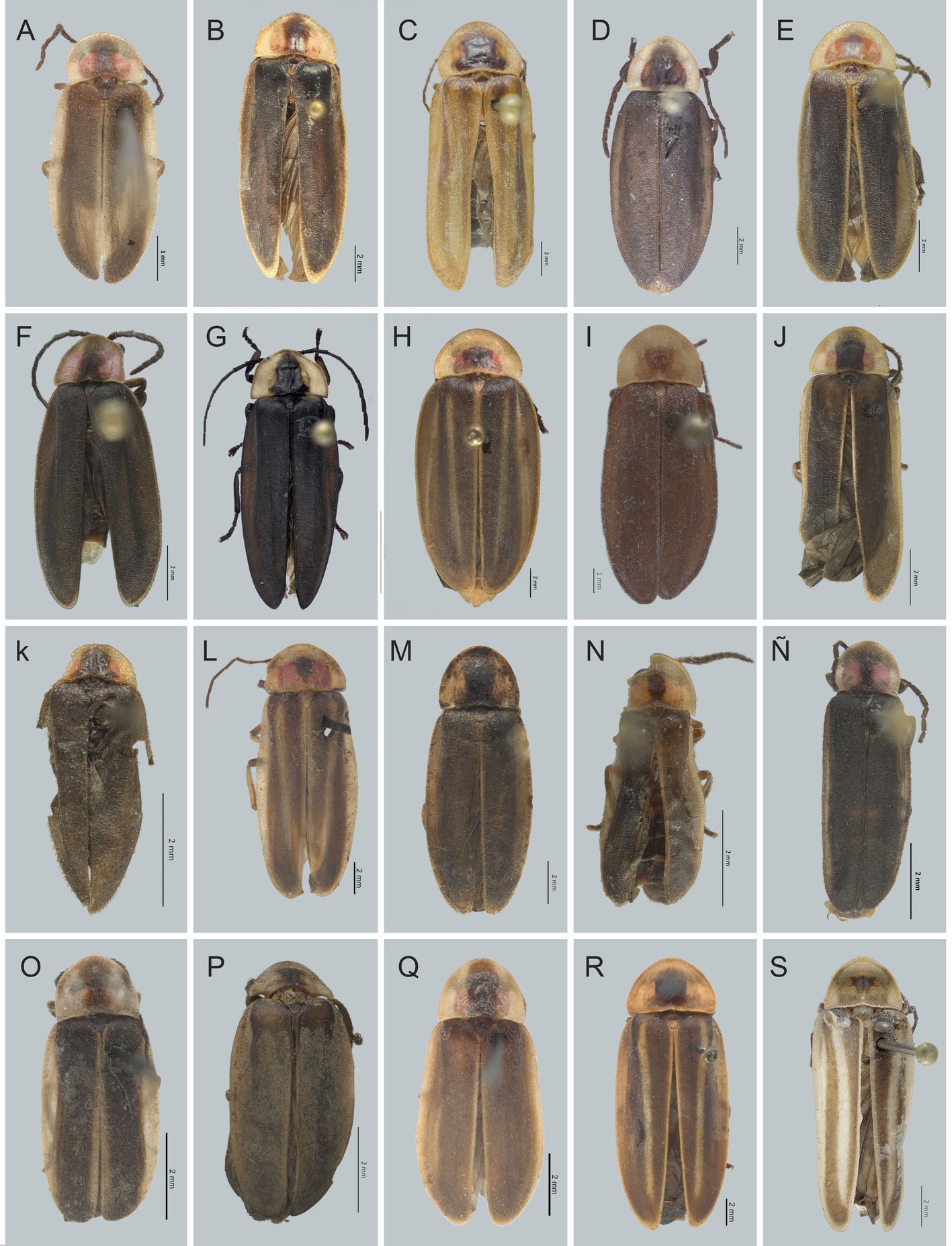
Figura 5. Vista dorsal de especies de Photinus. A) Photinus acremophallus,B) P. aldretei, C) P. alvarezi, D) P. asiainae, E) P. chaaci, F) P. chantzinae, G) P. choonghayi, H) P. cuasicongruus, I) P. dhipaki, J) P. escalanteae, K) P. estebani, L) P. gliscens, M) P. homerogomezi, N) P. janisae, Ñ) P. juarezae, O) P. lekoalloios, P) P. mictlantecuhtli, Q) P. noguerai, R) P. paracongruus, S) P. perezi.
Resumen taxonómico
Etimología. Dedicado al dios Mictlantecuhtli, “el señor del lugar de los muertos”, al que adoraban los totonacas de acuerdo con los vestigios arqueológicos encontrados en El Zapotal, Veracruz.
Material examinado. Holotipo macho. México: Veracruz: Microondas San Juan, S. of Fortin, 07-VII-1992. M. C. Thomas Beatingv. | Photinus sp. (Laporte, 1833) | CQR. 51747 | Colección del Instituto de Biología, UNAM, México, D.F. | COL.TIP-03966.
Photinus noguerai Zaragoza-Caballero, 1996
Figs. 5Q, 6Q, 12B, 13B, 14B
Photinus (Photinus) noguerai Zaragoza-Caballero, 1996: 137
Macho. Talla: largo 10.65 mm, ancho 4.08 mm Cuerpo ovoide, color castaño, mancha negra del pronoto paralela; élitros uniformemente coloreados; aparato luminoso presente en los esternitos 5-6, un poco más largos que los precedentes, con puntuaciones laterales, borde posterior del 7, cóncavo, 8 espatulado; edeago (figs. 12B, 13B, 14B) robusto más largo que lóbulos laterales, éstos en forma de “S”, lóbulo medio cilíndrico, con las excrecencias cortas, curvadas y separadas.
Distribución: Veracruz.

Figura 6. Vista ventral de especies de Photinus. A) Photinus acremophallus, B) P. aldretei, C) P. alvarezi, D) P. asiainae, E) P. chaaci, F) P. chantzinae, G) P. choonghayi, H) P. cuasicongruus, I) P. dhipaki, J) P. escalanteae, K) P. estebani, L) P. gliscens, M) P. homerogomezi, N) P. janisae, Ñ) P. juarezae, O) P. lekoalloios, P) P. mictlantecuhtli, Q) P. noguerai, R) P. paracongruus, S) P. perezi.
Photinus paracongruus Zaragoza-Caballero, 1996
Figs. 5R, 6R, 12C, 13C, 14C
Macho. Talla: largo 21.75 mm, ancho 8.38 mm. Cuerpo ovoide, color castaño, mancha negra del pronoto casi cuadrada; élitros con una banda media y sutural amarillenta; aparato luminoso presente en esternitos 5-6, tan largos como los precedentes, con puntuaciones laterales, borde posterior del 7, cóncavo, 8 espatulado; edeago (figs. 12C, 13C, 14C) con pieza basal más larga que lóbulos laterales, éstos en vista lateral curvados, lóbulo medio corto, distalmente atenuado, con las excrecencias largas, cilíndricas, y medianamente cerca.
Distribución: México: Veracruz.
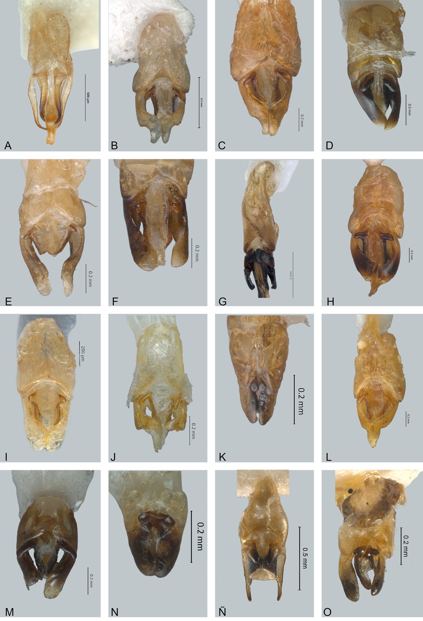
Figura 7. Vista dorsal de edeagos de Photinus. A) Photinus acremophallus, B) P. aldretei, C) P. alvarezi, D) P. asiainae, E) P. chaaci, F) P. chantzinae, G) P. choonghayi, H) P. cuasicongruus, I) P. dhipaki, J) P. escalanteae, K) P. estebani, L) P. gliscens, M) P. homerogomezi, N) P. janisae, Ñ) P. juarezae, O) P. lekoalloios.
Photinus parvulus Gorham, 1881
Macho. Talla: largo 4.5-5.00 mm. Cuerpo alargado, color gris oscuro, pronoto negro con margen blanquecino y con una impresión alargada; élitros negros; esternitos blanquecinos; antenas largas rebasando el cuarto esternito.
Distribución: México: Veracruz.

Figura 8. Vista ventral de edeagos de Photinus. A) Photinus acremophallus, B) P. aldretei, C) P. alvarezi, D) P. asiainae, E) P. chaaci, F) P. chantzinae, G) P. choonghayi, H) P. cuasicongruus, I) P. dhipaki, J) P. escalanteae, K) P. estebani, L) P. gliscens, M) P. homerogomezi, N) P. janisae, Ñ) P. juarezae, O) P. lekoalloios.
Photinus perezi Zaragoza-Caballero, 1995
Figs. 5S, 6S, 12D, 13D, 14D
Macho. Talla: largo 12.51 mm, ancho 4.19 mm. Cuerpo alargado, color castaño, mancha negra del pronoto triangular; élitros amarillentos con una banda humeral y otra sutural negra; aparato luminoso presente en esternitos 5-6, más largos que los precedentes, con puntuaciones laterales, borde posterior del 7 cóncavo, 8 ojival; edeago (figs. 12D, 13D, 14D) con pieza basal más larga que lóbulos laterales, éstos curvados en vista lateral, lóbulo medio corto, con excrecencias representadas por 2 prominencias laterales.
Distribución: México: Veracruz.

Figura 9. Vista lateral de edeagos de Photinus. A) Photinus acremophallus, B) P. aldretei, C) P. alvarezi, D) P. asiainae, E) P. chaaci, F) P. chantzinae, G) P. choonghayi, H) P. cuasicongruus, I) P. dhipaki, J) P. escalanteae, K) P. estebani, L) P. gliscens, M) P. homerogomezi, N) P. janisae, Ñ) P. juarezae, O) P. lekoalloios.
Photinus perotensis Zaragoza-Caballero, 1996
Figs. 10A, 11A, 12E, 13E, 14E
Macho. Talla: largo 14.16 mm, ancho 5.66 mm. Cuerpo ovoide, color negro, mancha negra del pronoto casi cuadrada; élitros negros; sin aparato luminoso, esternitos 5-6, tan largos como los precedentes, sin puntuaciones laterales, borde posterior del 7 convexo, el 8 ojival; edeago (12E, 13E, 14E) con pieza basal tan larga como lóbulos laterales, éstos asimétricos, lóbulo medio asimétrico, con excrecencias casi esféricas y basalmente cercanas.
Distribución: México: Veracruz.
Photinus phalloentis Zaragoza-Caballero, 1996
Figs. 10B, 11B, 12F, 13F, 14F
Macho. Talla: largo 15.17 mm, ancho 6.12 mm. Cuerpo ovoide, color negro, mancha negra del pronoto alargada; élitros negros; sin aparato luminoso, esternitos 5-6, tan largos como los precedentes, sin puntuaciones laterales, borde posterior del 7 cóncavo, 8 ojival; edeago (figs. 12F, 13F, 14F) con pieza basal asimétrica más corta que los lóbulos laterales, éstos asimétricos, lóbulo medio asimétrico, con excrecencias casi esféricas desiguales y basalmente cercanas.
Distribución: México: Veracruz.
Photinus plumbeus Gorham, 1880
Figs. 10C, 11C, 12G, 13G, 14G
Macho. Talla: largo 6.00 mm, ancho 2.88 mm. Cuerpo alargado, paralelo, de color castaño; pronoto blanquecino, disco acanalado; élitros con márgenes lateral y sutural blanquecinos; aparato luminoso ocupando esternitos 5-6; edeago (figs. 12G, 13G, 14G) con pieza basal simétrica, lóbulos laterales en vista lateral apicalmente muy angostos, lóbulo medio cónico, con excrecencias cortas, lobuladas y separadas.
Distribución: México: Veracruz.
Photinus poncianoae Zaragoza-Caballero y Pérez-Flores, sp. nov.
Figs. 10D, 11D, 12H, 13H, 14H
http://zoobank.org:act:C72F1F28-D209-4259-A1F6-078
D34239575
Macho. Talla: largo 10.19 mm, ancho 4.00 mm. Color negro, pronoto con una mancha negra basal casi cuadrada, ápice y lados del pronoto ferruginosos, margen lateral y sutural de los élitros del mismo color, coxas, fémures, base de tibias y margen posterior del esternito 5; aparato luminoso en esternitos 5-7. Cabeza: espacio interocular (0.68 mm), plano, paralelo, con integumento rugoso, brillante y diminutas sedas decumbentes; frente vertical, distancia interantenal (0.22 mm), más angosta que fosita antenal (0.55 mm); ojos finamente facetados, semiesféricos, más largos (0.46 mm) que anchos (0.33 mm); antenas filiformes, largas, escapo alcanzando 0.70 mm de longitud, claviforme, más largo que los 2 siguientes juntos, segundo corto (0.19 mm), tercero de 0.36 mm, del cuarto al décimo de 0.46 mm, undécimo alcanza 0.40 mm; sutura frontoclipeal membranosa; clípeo trapezoidal, borde anterior cóncavo, superficie rugosa, con sedas cortas; mandíbulas falcadas; sin sedas basales; palpómero maxilar apical securiforme; palpómero labial fusiforme. Tórax: pronoto más ancho (3.18 mm) que largo (2.00 mm), semicircular, borde posterior recto, ángulos posteriores romos, lados ampliamente explanados, con poros glandulares ordenados en el margen, más abundantes en parte anterior del disco, superficie brillante, pilosidad decumbente; escutelo espatulado, con borde posterior romo, superficie rugosa, pilosidad decumbente; élitros poco más de 4 veces más largos (8.18 mm) que anchos (2.00 mm), superficie rugosamente punteada, opaca, con 2 tipos de pilosidad decumbente, una larga y erecta, otra muy pequeña; epipleura angosta; espiráculos respiratorios mesotorácicos no tubulares; patas cortas, pro y mesopatas semejantes entre sí, metapatas un poco más largas, fémures casi fusiformes, tibias un poco dilatadas al ápice, borde externo no crenulado, espinas tibiales 2-2-2 de longitud subigual (0.17 mm) tarsómeros lateralmente comprimidos, primer metatarsómero más largo (0.58 mm) que los 2 siguientes juntos (0.40 mm), cuarto bífido, cubriendo gran parte del quinto, uñas simples. Abdomen: esternitos 1 y 2 de 0.74 mm, esternito 3 y 4 de 0.59 mm, presentan parte media del borde posterior recta, ángulos posteriores casi rectos, esternito 5 de 0.74 mm, 6 de 1.29 mm sin puntuaciones estigmatiformes, parte media del borde posterior ondulado y ángulos posteriores romos, esternito 7 de 0.74 mm con borde posterior emarginado, esternito 8 de 1.18 mm, ojival, tergitos apicales no superpuestos; edeago (figs. 12H, 13H, 14H ) con pieza basal simétrica, más larga (0.72 mm) que lóbulos laterales (0.58 mm), éstos modificados para recepción de excrecencias dorso basales, lóbulo medio cilíndrico, más corto que los lóbulos laterales, excrecencias lobuladas, divergentes y basalmente separadas. Hembra desconocida.
Resumen taxonómico
Etimología. El nombre está dedicado a Guadalupe Ponciano, entrañable compañera de andanzas en el campo mexicano.
Material examinado. Holotipo macho: México, Veracruz, Rancho La Camelia, 12-V-1994, S. Zaragoza, A. Mendoza coll. | CQR. | COL.TIP-03967.
*Photinus productus Gorham, 1881. En Zaragoza-Caballero et al. (2020).
Distribución: Chiapas, Oaxaca, Puebla y Veracruz.
Photinus pulchellus Gorham, 1880
Figs. 10E, 11E, 12I, 13I, 14I
Macho. Talla: largo 9.02 mm, ancho 3.20 mm. Cuerpo ovoide, de color negro plomizo. Cabeza con vértex plano; antenas filiformes, largas, rebasa segundo esternito; clípeo casi rectangular, con borde anterior ligeramente escotado; palpos labiales con último artejo un tanto securiforme; pronoto más ancho que largo, borde anterior semicircular, ángulos posteriores casi rectos; élitros paralelos, entre 4 y 5 veces más largos que anchos; abdomen sin puntuaciones estigmatiformes, borde posterior del sexto esternito ligeramente hendido en el macho; aparato luminosos en macho ocupando toda la superficie ventral de los segmentos 5 y 6, en hembras reducido a una mancha sobre el quinto; edeago (figs. 12I, 13I, 14I) con lóbulos laterales casi en forma de S, con parte distal membranosa, lóbulo medio con excrecencias dorsobasales reducidas; orificio medio terminal.
Distribución: México: Veracruz.
Photinus reichei Gorham, 1881
Figs. 10F, 11F, 12J, 13J, 14J
Macho. Talla: largo 9 mm, ancho 3.5 mm, Cuerpo alargado-ovalado, negro-castaño; pronoto amarillo, disco negro, convexo, brillante, acanalado, castaño a los lados; élitros negro castaño, sutura amarilla muy angosta; abdomen con 3 últimos segmentos amarillos tanto dorsal como ventralmente; edeago (figs. 12J, 13J, 14J) corto, robusto, pieza basal simétrica, lóbulos laterales modificados para recepción de las excrecencias cortas, lobuladas y separadas del lóbulo medio cilíndrico.
Distribución: México: Oaxaca y Veracruz.
Photinus staku Zaragoza-Caballero y Vega-Badillo, sp. nov.
Figs. 10G, 11G, 12K, 13K, 14K
http://zoobank.org:act:1C23ED6D-7AB3-4315-BA38-329
CD9C5F9C2
Macho. Talla: largo 8.54 mm, ancho 2.72 mm. Color castaño con excepción del pronoto y margen lateral de élitros amarillentos, disco con una franja central café y 2 máculas rosas; procoxas, metacoxas y fémures ambarinos; aparato luminoso ocupando esternitos 5-6. Cabeza: espacio interocular (0.62 mm) cóncavo, casi paralelo, integumento brillante, liso y piloso; frente vertical, distancia interantenal (0.12 mm) más angosta que lo ancho de fosita antenal (0.22 mm); ojos finamente facetados, semiesféricos, prominentes, más largos (0.51 mm) que anchos (0.38 mm); antenas filiformes (3.5 mm), 2 veces más largas que pronoto, sobrepasa borde posterior del metasterno, escapo alcanzando 0.50 mm de longitud, claviforme, tan largo como 2 antenitos siguientes juntos, segundo corto (0.15 mm), del tercero al décimo de 0.35 mm, undécimo alcanza 0.50 mm; sutura frontoclipeal, membranosa, casi recta; clípeo trapezoidal, borde anterior recto, superficie con grandes sedas irregularmente distribuidas; mandíbulas falcadas, delgadas con sedas en su borde externo, uniformemente arqueadas; palpómero maxilar apical securiforme; palpómero labial casi triangular. Tórax: pronoto más ancho (2.00 mm) que largo (1.91 mm), ojival, borde posterior recto, ángulos posteriores obtusos, disco convexo, lados cóncavos, explanados, con poros glandulares en márgenes, más abundantes anteriormente, superficie brillante, pilosidad abundante, procumbente; escutelo triangular, con borde posterior redondeado, superficie brillante, gruesamente punteada y pilosidad procumbente; élitros largos casi paralelos, 4.95 veces más largos (6.73 mm) que anchos (1.36 mm), superficie rugosa, brillante, pilosidad corta, abundante, decumbente; epipleura ancha; espiráculos respiratorios mesotorácicos tubulares; patas cortas, esbeltas pro y mesopatas semejantes entre sí, metapatas más largas, fémures fusiformes aplanados, tibias aplanadas un poco dilatadas al ápice, borde externo crenulado y margen apical entero, espinas tibiales 2-2-2 de longitud semejante (0.12 mm), tarsómeros lateralmente comprimidos, primer metatarsómero (0.37 mm) más largo que 2 siguientes juntos (0.30 mm), cuarto bífido, cubriendo 2 tercios del quinto, uñas simples. Abdomen: esternito 1 y 2 de 0.50 mm, 3 y 4 de 0.42 mm, presentan parte media del borde posterior ligeramente ondulada y ángulos posteriores casi rectos, esternito 5 de 0.63 mm, 6 de 0.75 mm sin poros estigmatiformes, parte media del borde posterior ondulados, ángulos posteriores romos, esternito 7 de 0.30 mm con borde posterior escotado y ángulos posteriores redondos, esternito 8 de 0.38 mm, ojival, con superficie excavada y borde posterior romo; pigidio con borde posterior romo; edeago (figs. 12K, 13K, 14K) con pieza basal simétrica, más larga (0.45 mm) que lóbulos laterales (0.37 mm), con borde posterior cóncavo; lóbulo medio cuadrado, con parte dorsal y ventral esclerosada, excrecencias dorso basales como lóbulos cortos, casi transversos, orificio medio apical, lóbulos laterales más largos que lóbulo medio, anchos en vista lateral, arqueados hacia la parte dorsal, ápice proyectado hacia arriba, sin modificaciones para la recepción de excrecencias del lóbulo medio. Hembra desconocida.
Resumen taxonómico
Etimología. Dedicado al dios totonaca Staku “las Estrellas” vigilante que cuida durante el día y la noche para que no revivan las piedras y los árboles, que para los totonacas eran almas dormidas.
Material examinado. Holotipo macho. México: Veracruz, Río de los Pescados 24 mi. S. Jalapa. 22-VIII-1977, 540 m snm. E. I. Schlinger | CQR. 51858 | COL.TIP-03968. Paratipo macho, México: Veracruz, Yecuatla, 25-III-1997. E. González | CQR. 51859 | COL.TIP-03969.
Photinus tenuilineatus Zaragoza-Caballero, 1996
Figs. 10H, 11H, 12L, 13L, 14L
Macho. Talla: largo 8.27 mm, ancho 2.72 mm. Cuerpo ovoide, color castaño, mancha negra del pronoto alargada, dividida por una franja rojiza; élitros castaño, con banda marginal, sutural y humeral amarillentas, ésta última apenas marcada; aparato luminoso en esternitos 5-6, más largos que precedentes, con puntuaciones laterales, borde posterior del 7 cóncavo, 8 espatulado; edeago (figs. 12L, 13L, 14L) con pieza basal simétrica tan larga como lóbulos laterales, éstos con ápice lateralmente dirigido; lóbulo medio alargado, comprimido, sin excrecencias dorso basales, con ápice bífido.
Distribución: México: Veracruz.
*Photinus tlapacoyanensis Zaragoza-Caballero, 1996. En Zaragoza-Caballero et al. (2020).
Distribución: Hidalgo, Puebla y Veracruz.
*Photinus tuxtlaensis Zaragoza-Caballero, 1995. En Zaragoza-Caballero et al. (2020).
Distribución: Campeche, Hidalgo, Oaxaca, Quintana Roo, San Luis Potosí, Tabasco, Tamaulipas, Veracruz y Yucatán.
Photinus vezlirai Zaragoza-Caballero y Domínguez-León, sp. nov.
Figs. 10I, 11I, 12M, 13M, 14M
http://zoobank.org:act:FDCDE956-B0BF-4B88-885D-38721EBACA73
Macho. Talla: largo 7.82 mm, ancho 2.59 mm. Color pardo a excepción del pronoto que es de un color ambarino en la parte media con una mancha café y 2 maculas rosas rodeando la anterior; procoxas, metacoxas y fémures ambarinos con ápice de color café; aparato luminoso ocupando únicamente esternito 6. Cabeza: espacio interocular (0.62 mm), cóncavo, paralelo, integumento brillante, chagrinado y piloso; frente vertical, distancia interantenal (0.08 mm) un poco más grande que el ancho de la fosita antenal (0.12 mm); ojos finamente facetados, esféricos, prominentes, más largos (0.82 mm) que anchos (0.49 mm); antenas filiformes (3.52 mm), 2 veces más largas que pronoto, sobrepasa borde posterior del metaesterno, escapo alcanzando 0.49 mm de longitud, claviforme, tan largo como 2 antenitos siguientes juntos, segundo corto (0.17 mm), del quinto al undécimo de 0.3 mm; sutura frontoclipeal membranosa, cóncava; clípeo con borde anterior recto, superficie con grandes sedas irregularmente distribuidas; mandíbulas falcadas, esbeltas; palpómero maxilar apical ovado; palpómero labial triangular. Tórax: pronoto más ancho (2.22 mm) que largo (1.52 mm), semicircular, bordes laterales casi paralelos en su mitad basal, borde posterior convexo en medio, ángulos posteriores rectos, disco convexo, lados angostamente explanados, con poros glandulares en los márgenes, superficie brillante, con abundante pilosidad, decumbente y procumbente, excepto en disco medio; escutelo trapezoidal, superficie brillante, con escasa puntuación oblicua y pilosidad procumbente; élitros largos, paralelos, un poco menos de 4 veces más largos (6.3 mm) que anchos (1.25 mm), superficie rugosa, opaca; pilosidad escasa y decumbente; epipleura reducida; espiráculos respiratorios mesotorácicos tubulares; patas largas, pro y mesopatas semejantes entre sí, fémures fusiformes, tibias dilatadas al ápice, borde externo liso, espinas tibiales 2-2-2 de longitud semejante (0.05 mm), primer metatarsómero un poco más largo (0.3 mm) que 2 siguientes juntos (0.28 mm), el cuarto bífido, cubriendo parte del quinto, uñas simples. Abdomen: esternitos 1 y 2 de 0.23 mm, 3 y 4 de 0.8 mm, presentan parte media del borde posterior emarginada, ángulos posteriores casi rectos, esternito 5 de 0.35 mm y 6 de 0.51 mm con poros estigmatiformes, parte media emarginada y ángulos posteriores romos, esternito 7 de 0.88 mm con parte media emarginada y ángulos posteriores redondeados; edeago (figs. 12M, 13M, 14M) con pieza basal simétrica, un poco más larga (0.46 mm), que los lóbulos laterales (0.28 mm), con borde posterior cóncavo, lóbulo medio cilíndrico, no esclerotizado visto dorsalmente, excrecencias dorso-basales como lóbulos cortos, paralelos, orientados y pegados a lóbulos laterales, orificio medio ubicado apicalmente, lóbulos laterales un poco más largos que lóbulo medio, anchos en vista lateral, ápice proyectado dorsalmente, con punta roma y ancha poco esclerotizada. Hembra desconocida.
Resumen taxonómico
Etimología. El nombre específico es formado mediante la combinación de los apellidos del ambientalista Adán Vez Lira, como un breve homenaje a quien durante muchos años defendió la flora y fauna de los humedales, manglares y dunas de La Mancha, Veracruz.
Material examinado. Holotipo macho. México: Veracruz: Laguna Sto. Domingo, 4 km NO Huatusco, 09-VII-2000, 19°09’50” N, 97°00’267” O | Col. S. Zaragoza C. | Photinus sp. (Laporte, 1833) | CQR. 52237 | COL.TIP-03970.
*Photinus vulgatus Olivier, 1907. En Zaragoza-Caballero et al. (2023).
Distribución: Michoacán, Quintana Roo y Veracruz.
Photinus xochiquetzalae Zaragoza-Caballero y Aquino-Romero, sp. nov.
Figs. 10J, 11J, 12N, 13N, 14N
http://zoobank.org:act:73AD585B-D9DA-49DE-8749-692A8D1C331A
Macho. Talla: largo 9.51 mm, ancho 3.46 mm. Color ambarino, con excepción del disco pronotal, que cuenta con una mancha rosa en medio y 3 manchas pardas, 2 laterales pequeñas y una central más alargada; escutelo con una mancha triangular rosa anteriormente y en medio una mancha circular ambarina; base superior del élitro, cabeza, tibias y coxas que ambarinos; aparato luminoso ocupando esternitos 5-6. Cabeza: espacio interocular (1.73 mm), plano, integumento brillante, chagrinado y piloso; frente vertical, distancia interantenal (0.72 mm), más angosta que el ancho de la fosita antenal; ojos finamente facetados, semiesféricos, prominentes, más anchos (0.77 mm) que largos (0.14 mm); antenas filiformes cortas, 1.7 veces más largas que pronoto, alcanza borde posterior de la procoxa, escapo alcanzando 0.97 mm de longitud, claviforme, más pequeño que 2 antenitos siguientes juntos, segundo corto (0.52 mm), tercero al undécimo de 0.44 mm; sutura frontoclipeal no membranosa, cóncava; clípeo oval, borde anterior convexo, superficie lisa con sedas cortas irregularmente distribuidas; mandíbulas falcadas, esbeltas, curveadas; palpómero maxilar apical securiforme; palpómero labial securiforme. Tórax: pronoto más ancho (2.82 mm) que largo (2.18 mm), semicircular, borde posterior cóncavo, borde anterior semicircular, ángulos posteriores rectos, disco convexo, explanaciones laterales evidentes, más amplias en parte superior, con poros glandulares en márgenes, superficie brillante, pilosidad ligeramente más abundante en parte anterior, decumbente; escutelo espatulado, con borde posterior acuminado, superficie brillante, punteado y pilosidad abundante, pequeña y procumbente; élitros largos, paralelos, 4 veces más largos (7.73 mm) que anchos (1.88 mm), superficie brillosa, integumento rugoso, pilosidad pequeña y decumbente; epipleura reducida, más estrecha en la base; espiráculos respiratorios mesotorácicos tubulares; patas cortas, fémures fusiformes, lateralmente aplanados, meso y metafémures más alargados, semejantes entre sí, tibias dilatadas al ápice, protibia con ápice ligeramente hendido, tarsómeros lateralmente comprimidos, primer metatarsómero ligeramente más largo (0.25 mm) que 2 siguientes juntos (0.24 mm), cuarto bífido, cubriendo parte del quinto, uñas simples. Abdomen: longitud de esternitos 1-3 de 0.23 mm, esternito 4 de 0.26 mm, ángulos posteriores casi rectos, esternito 5 de 0.32 mm y 6 de 0.79 mm, con puntuaciones estigmatiformes, presentan parte media del borde posterior emarginada y ángulos posteriores romos, esternito 7 de 0.88 mm con borde posterior escotado y ángulos posteriores redondos, esternito 8 de 0.61 mm, ojival, con superficie excavada y borde posterior romo; pigidio con borde posterior redondeado; edeago (figs. 12N, 13N, 14N) con pieza basal simétrica, más corta (0.10 mm) que lóbulos laterales (0.18 mm), con borde posterior escotado, lóbulo medio cilíndrico, con superficie dorsal membranosa, integumento lateral liso y esclerosado, porción apical fuertemente hendida, superficie ventral con base esclerosada y parte apical membranosa, orificio medio abierto apicalmente, excrecencias dorso basales simétricas, separadas, como lóbulos cortos, fusionadas en la parte basal, lóbulos laterales simétricos, más largos que lóbulo medio, dilatados basalmente, robustos en vista lateral, sin modificaciones para recepción de excrecencias del lóbulo medio. Hembra desconocida.
Resumen taxonómico
Etimología. El nombre hace referencia a la diosa tolteca Xochiquetzal, diosa de la belleza, las flores, el placer amoroso y las artes, que era adorada por pobladores toltecas en algunas regiones de Xalapa, Veracruz.
Material examinado. Holotipo macho. México: Veracruz: Río de los Pescados, 24 mi S. Jalapa, VIII-22-1977, 540 m snm, E.I. Schlinger. | CQR 51861 | Colección del Instituto de Biología, UNAM, México, CDMX. | COL.TIP-03971.
Photinus xonamancae Zaragoza-Caballero, 1996
Figs. 10K, 11K, 12Ñ, 13Ñ, 14Ñ
Macho. Talla: largo 6.91 mm, ancho 2.26 mm. Cuerpo ovoide, color castaño, mancha negra del pronoto fungiforme; élitros negros, con margen lateral y sutural amarillo; aparato luminoso en esternitos 5-6, tan largos como precedentes, con puntuaciones laterales, borde posterior del 7 cóncavo, 8 ojival; edeago (figs. 12Ñ, 13Ñ, 14Ñ) con pieza basal simétrica, más larga que lóbulos laterales, estos, en vista lateral casi triangulares, con ápice redondo, lóbulo medio cónico, excrecencias dorso-basales pequeñas asimétricas y separadas.
Distribución: México: Veracruz.
*Photinus zongolicaensis Zaragoza-Caballero y Domínguez-León, 2020. En Zaragoza-Caballero et al. (2020).
Distribución: Chiapas, Puebla y Veracruz.
*Pyropyga Motschulsky, 1852
Especie tipo: Lampyris nigricans Say, 1823: 179
Blackwelder (1945: 353), Blackwelder y Arnett (1974: 6), Green (1948: 68, 1961: 61), Gorham (1880a: 22, 1881: 38), Lacordaire (1857: 321), LeConte (1852: 333, 1881: 32), McDermott (1964: 30, 1966: 59), Motschulsky (1852: 28), Olivier (1907: 18, 1911: 71), Zaragoza-Caballero (1993: 139), Zaragoza-Caballero et al. (2020: 9) y Zaragoza-Caballero, López-Pérez et al. (2023: 71).
Diagnosis en Zaragoza-Caballero et al. (2023).
*Pyropyga alticola Green, 1961. En Zaragoza-Caballero et al. (2023).
Distribución: Chiapas, Ciudad de México, Coahuila, Estado de México, Guerrero, Hidalgo, Morelos, Oaxaca, Puebla y Veracruz.
*Pyropyga cordobana Green, 1961. En Zaragoza-Caballero et al. (2023).
Distribución: Chiapas, Jalisco, Morelos, San Luis Potosí, Puebla y Veracruz.
*Pyropyga extensa Green, 1961. En Zaragoza-Caballero et al. (2023).
Distribución: Ciudad de México, Chiapas, Durango, Puebla, Quintana Roo, Tamaulipas y Veracruz.
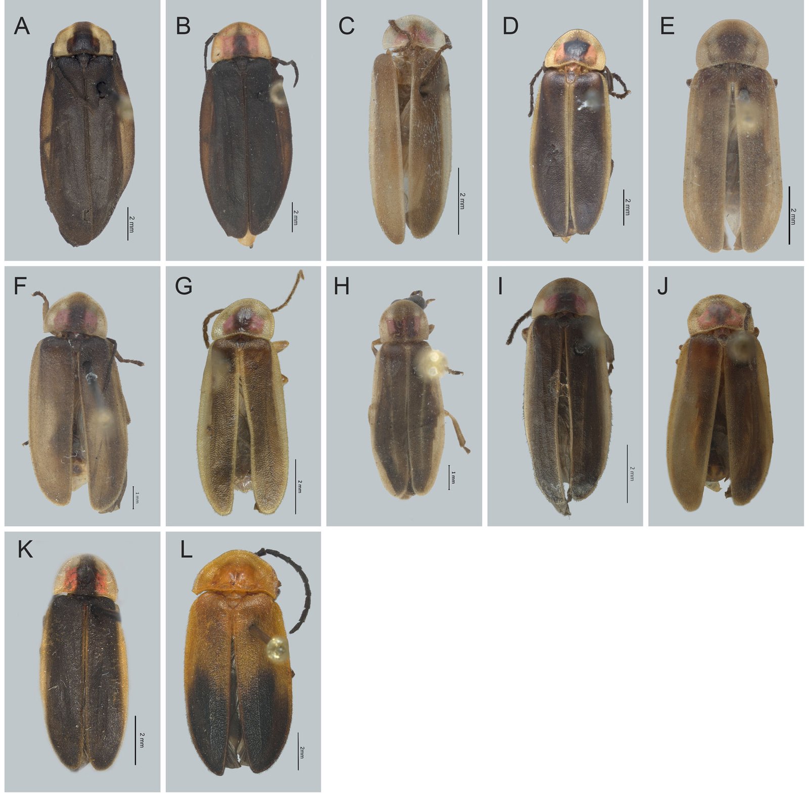
Figura 10. Vista dorsal de especies de Photinus. A) Photinus perotensis, B) P. phalloentis, C) P. plumbeus, D) P. poncianoae, E) P. pulchellus, F) P. reichei,G) P. staku,H) P. tenuilineatus, I) P. vezlirai, J) P. xochiquetzalae, K) P. xonamancae, L) Lucidota discolor.
*Pyropyga minuta (LeConte, 1851). En Zaragoza-Caballero et al. (2023).
Ellychnia minuta LeConte, 1851: 333
Distribución: Ciudad de México, Chiapas, Coahuila, Colima, Durango, Estado de México, Guanajuato, Guerrero, Hidalgo, Jalisco, Michoacán, Morelos, Nayarit, Nuevo León, Oaxaca, Puebla, Quintana Roo, San Luis Potosí, Tamaulipas y Veracruz.
*Pyropyga modesta Green, 1961. En Zaragoza-Caballero et al. (2023).
Distribución: Chiapas, Coahuila, Colima, Guerrero, Hidalgo, Jalisco, Michoacán, Morelos, Nayarit, Nuevo León, Oaxaca, Puebla, San Luis Potosí, Tamaulipas y Veracruz.
*Pyropyga nigricans (Say, 1823). En Zaragoza-Caballero et al. (2023).
Lampyris nigricans Say, 1823: 179
Distribución: Aguascalientes, Baja California Sur, Chiapas, Chihuahua, Ciudad de México, Durango, Estado de México, Guanajuato, Hidalgo, Jalisco, Michoacán, Morelos, Nayarit, Oaxaca, Puebla, San Luis Potosí, Sinaloa, Sonora y Veracruz.
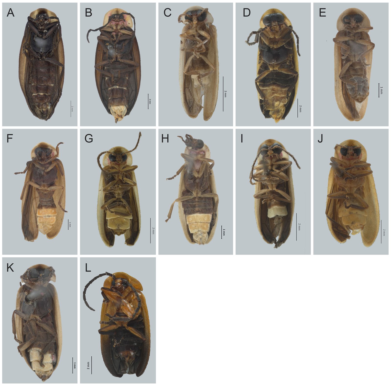
Figura 11. Vista ventral de especies de Photinus. A) Photinus perotensis, B) P. phalloentis, C) P. plumbeus, D) P. poncianoae, E) P. pulchellus, F) P. reichei, G) P. staku, H) P. tenuilineatus, I) P. vezlirai, J) P. xochiquetzalae, K) P. xonamancae, L) Lucidota discolor.
*Photinoides McDermott, 1963
Especie tipo: Photinoides penai McDermott, 1963: 86
Blackwelder y Arnett (1976: 12), McDermott (1964: 27, 1966: 48).
Diagnosis en Zaragoza-Caballero et al. (2023)
Photinoides bidenticauda (McDermott, 1958)
Photinus bidenticauda McDermott, 1958:25
Macho. Talla: largo 6.00 mm, ancho 1.9 mm. Cuerpo paralelo, castaño; antenas más largas que pronoto, ojival, rojizo, con una angosta banda oscura; escutelo amarillo; élitros marrones, con una costilla oblicua, ligeramente acuminados, margen lateral y sutural amarillo; aparato luminoso ocupando esternitos 5-6, más largos que precedente; pigidio más menos hexagonal con 2 proyecciones ventrales.
Distribución: México: Veracruz.
*Lucidota Laporte, 1833
Especie tipo: Lucidota banoni Laporte, 1833: 137
Blackwelder (1945: 353), Blackwelder y Arnett (1976: 4), Gorham (1880a: 15, 1881: 34), Green (1948: 68), Lacordaire (1857: 318), Laporte (1833: 136), LeConte (1881: 31), Leng y Mutchler (1922: 434), McDermott 1964: 31, 1966: 62), Motschulsky (1853: 41), Olivier (1907: 18, 1911: 70), Zaragoza-Caballero (1995a: 52), Zaragoza-Caballero et al. (2020: 8).
Diagnosis en Zaragoza-Caballero et al. (2020)
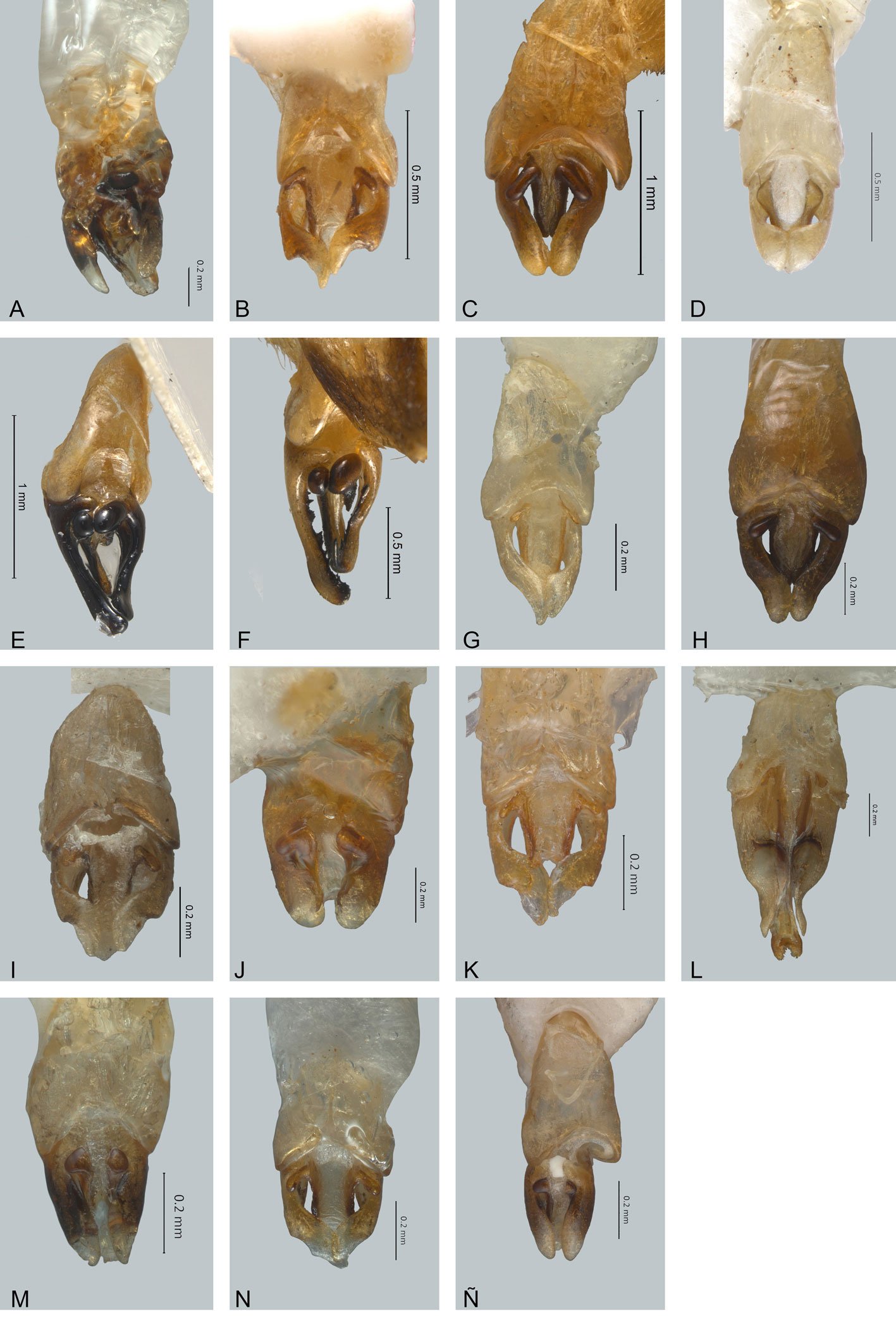
Figura 12. Vista dorsal de edeagos de Photinus. A)Photinus mictlantecuhtli, B) P. noguerai,C) P. paracongruus,D) P. perezi, E) P. perotensis,F) P. phalloentis,G) P. plumbeus,H) P. poncianoae,I) P. pulchellus,J) P. reichei, K) P. staku, L) P. tenuilineatus, M) P. vezlirai, N) P. xochiquetzalae, Ñ) P. xonamancae.
*Lucidota bella Gorham, 1880. En Zaragoza-Caballero et al. (2020)
Distribución: Campeche, Chiapas, Estado de México, Oaxaca, Tabasco y Veracruz.
Lucidota diaphanura Gorham, 1881
Talla: largo en machos y hembras de 12.00-15.00 mm. Cuerpo ancho, ovoide, negro opaco; pronoto semicircular, blanquecino, con margen oscuro, acanalado, con una mancha negra central; élitros, convexos; esternitos negros, los apicales blanquecinos.
Distribución: México: Veracruz.

Figura 13. Vista ventral de edeagos de Photinus. A)Photinus mictlantecuhtli, B) P. noguerai, C) P. paracongruus, D) P. perezi, E) P. perotensis, F) P. phalloentis, G) P. plumbeus, H) P. poncianoae, I) P. pulchellus, J) P. reichei, K) P. staku, L) P. tenuilineatus, M) P. vezlirai, N) P. xochiquetzalae, Ñ) P. xonamancae.
Lucidota discolor Gorham, 1881
Figs. 10L, 11L
Macho. Talla: largo 12.68 mm, ancho 5.37. Cuerpo alargado, ovoide, mitad anterior ferruginosa y posterior negra; esternitos negros, sin puntuaciones laterales, 7 en macho mucronado, 8 ojival de color ferruginoso; 7 con 2 pequeñas manchas blanquecinas laterales, en las hembras se encuentran en esternitos 5-6; pieza basal del edeago simétrica, más corta que lóbulos laterales, estos, apicalmente triangulares y con una proyección ventral, lóbulo medio más largo que laterales con ápice comprimido y curvado.
Distribución: México: Veracruz.
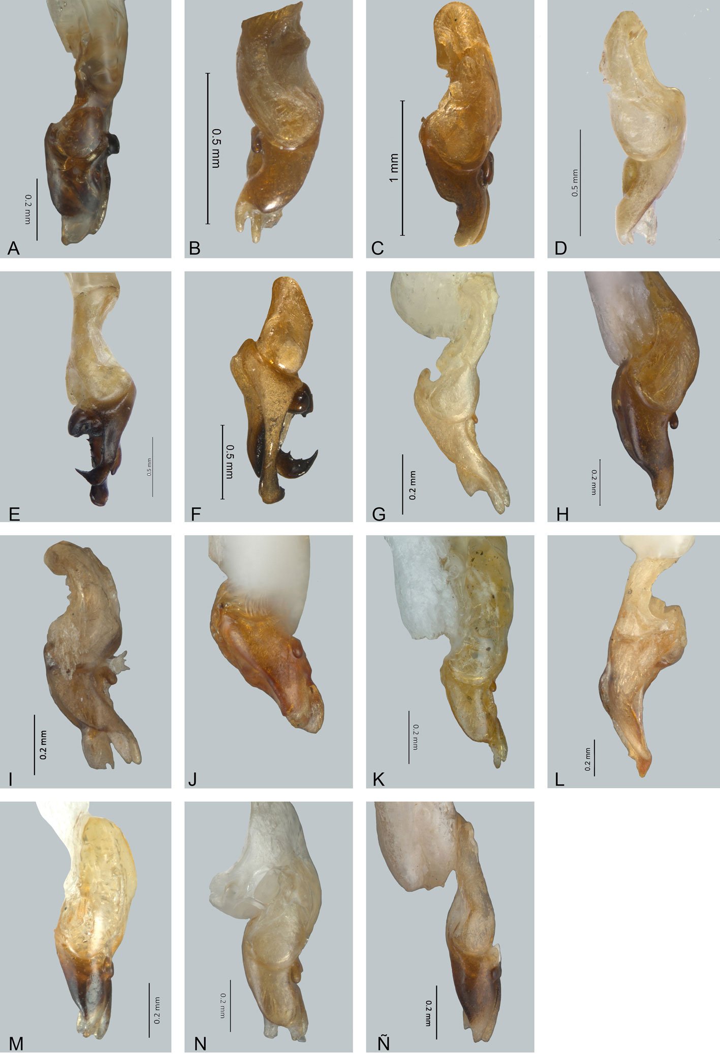
Figura 14. Vista lateral de edeagos de Photinus. A) Photinus mictlantecuhtli, B) P. noguerai, C) P. paracongruus,D) P. perezi,E) P. perotensis,F) P. phalloentis,G) P. plumbeus,H) P. poncianoae,I) P. pulchellus,J) P. reichei, K) P. staku, L) P. tenuilineatus, M) P. vezlirai, N) P. xochiquetzalae, Ñ) P. xonamancae.
Discusión
Estudios recientes han actualizado el estatus nomenclatural del género Photinus Laporte (Zaragoza-Caballero et al., 2020; Zaragoza-Caballero, Zurita-García et al., 2023). McDermott en 1966 registró 237 especies; por otro lado, Zaragoza-Caballero, Zurita-García et al. (2023) citan 396 especies, a partir de entonces se han descrito 51 especies (Gutiérrez-Carranza et al., 2023, 2024; Zaragoza-Caballero, Zurita-García et al., 2023) sumado a las 15 descritas en este trabajo Photinus se conforma de 462 especies siendo el género más diverso de Lampyridae,seguido de Luciola Laporte con 173 especies (Keller, 2024),el primero propio del continente Americano y el segundo distribuido en el Viejo Mundo.
Durante el estudio de Lampyridae en México (Zaragoza-Caballero et al., 2020; Zaragoza-Caballero, López-Pérez et al., 2023), se descubrió un notable polimorfismo entre las especies de Photinus registradas en el país. Esta variación se manifiesta en la coloración y tamaño, desde especies pequeñas como P. ojiviformis Zaragoza-Caballero y Rodríguez-Mirón de 3.43 × 0.87 mm, hasta ejemplares más grandes como P. congruus Zaragoza-Caballero de 21.72 × 8.4 mm de largo y ancho, respectivamente. Entre sus especies, las hay de cuerpo escutiforme o paralelo. La forma del cuerpo se refleja en la relación de largo y ancho de los élitros, en los registros hemos encontrado desde 3.35 veces tan largo como ancho (P. advenus Olivier) hasta 7.64 [P. palaciosi (Zaragoza-Caballero)]. A su vez, esta relación —aparentemente— se manifiesta en la distribución altitudinal que alcanzan. Especies con el cuerpo ancho y corto, son concurrentes en alturas bajas como sucede con P. aliciae Zaragoza-Caballero (3.65) de las costas de Colima, Guerrero, Jalisco y Michoacán; las de cuerpo alargado y paralelo como P. gabicastanoae Gutiérrez-Carranza y Zaragoza-Caballero (8.5) se han registrado a 2,583 m snm. De las especies comentadas en este trabajo, los élitros en P. cuasicongruus Zaragoza-Caballero y P. juarezae Zaragoza-Caballero, pueden considerarse como ejemplo de esta situación. La primera, con cuerpo más menos ovoide, tiene una relación de 3.8 de largo/ancho en sus élitros y se le encuentra a una altura de 1,290 m snm, mientras que en P. juarezae, la relación es de 4.91 y se ubica a los 1,515 m snm.
En este trabajo, se evidencia la ausencia de nuevas especies o registros para los estados de Quintana Roo y Yucatán. A pesar de los esfuerzos que se han hecho para realizar estudios de la coleopterofauna de la zona del Caribe aún existen zonas poco estudiadas; en algunas zonas se cuentan con datos sobre familias puntuales como Melolonthidae, Passalidae y Scarabaeidae (Delgado et al., 2012; Halffter y Halffter 2009; Morón, 2001; Navarrete-Gutiérrez y Halffter, 2008; Reyes-Castillo 2000, 2002; Reyes-Novelo y Morón, 2005). Sin embargo, los listados de especies de Coleoptera en la zona del Caribe aún están lejos de ser completados y específicamente para Lampyridae, el material con el que se cuenta está basado en colectas esporádicas y publicaciones aisladas que resultan en el desconocimiento de la diversidad de luciérnagas que puede albergar. Por lo anterior, este estudio representa un primer avance en el conocimiento de luciérnagas
del Caribe.
Finalmente, es importante continuar con estudios específicos de luciérnagas en estados cuya diversidad permanece subestimada, como lo son Chiapas, Quintana Roo y Yucatán; dada su importancia como especie bandera y desde un punto de vista biológico y cultural, se requiere que distintos sectores impulsen medidas adecuadas para su protección y conservación (Lewis et al., 2021; Singh et al., 2020).
Agradecimientos
A Susana Guzmán del Laboratorio de Microscopía y Fotografía de la Biodiversidad, Instituto de Biología, UNAM por la ayuda técnica en la toma de fotografías. Así mismo, a Janis Vigil Razo por la toma de diferentes fotografías y a Tifereth Cruz Rico por su asistencia en la edición digital. Además, se agradece a Keita Matsumoto y Michael Geiser del Museo de Historia Natural de Londres por facilitarnos las fotos del ejemplar tipo de Magnoculus guatemalae y a Mark G. Volkovitsh del Instituto de Zoología de San Petersburgo por proporcionarnos las fotos del ejemplar tipo de Ellychnia albilatera. De igual manera, agradecemos a un revisor anónimo y a José Luis Navarrete Heredia quienes con sus comentarios enriquecieron este trabajo.
Apéndice. Lista de especies presentes en la región golfo-Caribe. El asterisco indica los taxones que ya se han mencionado en Zaragoza-Caballero et al. (2020) y Zaragoza-Caballero, López-Pérez et al. (2023).
Vesta Laporte, 1833
Vesta thoracica (Olivier, 1790)
Magnoculus McDermott, 1964
Magnoculus tlaloque Zaragoza-Caballero y Gutiérrez-Carranza, sp. nov.
Amydetes Illiger, 1807
Amydetes fastigiata Illiger, 1807
*Bicellonycha Motschulsky,1853
Bicellonycha albomarginata Zaragoza-Caballero, 1989
*Bicellonycha amoena (Gorham, 1880)
*Bicellonycha collaris (Gorham, 1880)
Bicellonycha crassa (Gorham, 1884)
*Bicellonycha discicollis (Gorham, 1881)
Bicellonycha facialis (Gorham, 1881)
*Bicellonycha gorhami Zaragoza-Caballero, 1989
*Bicellonycha limbata Pic, 1924
*Bicellonycha mexicana (Gorham, 1880)
Bicellonycha ruficollis (Gorham, 1880)
Bicellonycha stigmatica (Olivier, 1886)
*Photuris Dejean, 1833
*Photuris fulvipes (Blanchard, 1846)
*Photuris lugubris Gorham, 1881
Photuris mollis Gorham, 1880
*Photuris tenuisignathus Zaragoza-Caballero, 1995
Photuris trivittata Lloyd y Ballantyne, 2003
*Photuris versicolor (Fabricius, 1798)
*Pleotomus LeConte, 1861
*Pleotomus pallens LeConte, 1866
*Phaenolis Gorham, 1880
*Phaenolis alboterminatus Zaragoza-Caballero, 1995
Phaenolis mexicana McDermott, 1958
Phaenolis ustulata Gorham, 1880
*Tenaspis LeConte, 1881
Tenaspis gonzalenzis Zaragoza-Caballero, 1995
*Cratomorphus Motschulsky, 1853
*Cratomorphus concolor (Perty, 1830)
Cratomorphus leoneli Lima et al. 2021
Cratomorphus picipennis Gorham, 1881
*Cratomorphus signativentris Olivier, 1895
*Aspisoma Laporte, 1833
*Aspisoma aegrota (Gorham, 1880)
*Aspisoma depictum (Gorham, 1880)
*Aspisoma diaphana (Gorham, 1880)
*Aspisoma ignitum (Linnaeus, 1767)
Aspisoma lepidum (Gorham, 1881)
*Aspisoma pulchellum (Gorham, 1880)
Aspisoma quasidiaphana Zaragoza-Caballero, 1995
Aspisoma yucatanum Olivier, 1908
*Pyractomena Melsheimer, 1846
*Pyractomena angulata (Say, 1825)
Pyractomena striatella Gorham, 1880
Pyractomena vexillaria Gorham, 1881
*Aspisomoides Zaragoza-Caballero, 1995
*Aspisomoides bilineatum (Gorham, 1880)
*Aspisomoides costatum (Gorham, 1880)
*Photinus Laporte, 1833
Photinus acremophallus Zaragoza-Caballero y Gutiérrez-Carranza, 2018
*Photinus advenus Olivier, 1907
Photinus affinis Gorham, 1880
Photinus albicauda Gorham, 1881
Photinus aldretei Zaragoza-Caballero, 1996
Photinus ampliatus Olivier, 1907
*Photinus anagabrielae Zaragoza-Caballero y Gutiérrez-Carranza, 2020
*Photinus albolimbatus Gemminger, 1870:119 comb. rest.
Photinus alvarezi Zaragoza Caballero y Cifuentes-Ruiz, sp. nov.
Photinus asiainae Zaragoza Caballero y Aquino-Romero, sp. nov.
Photinus chaaci Zaragoza-Caballero y González-Ramírez, sp. nov.
Photinus chantzinae Zaragoza-Caballero y Cifuentes-Ruiz, sp. nov.
Photinus choonghayi Gutiérrez-Carranza y Zaragoza-Caballero, sp. nov.
*Photinus congruus Chevrolat, 1834
Photinus cordovae Gorham, 1881
*Photinus corrusca (Linnaeus, 1767)
Photinus cuasicongruus Zaragoza-Caballero, 1996
Photinus dhipaki Zaragoza-Caballero y López-Pérez, sp. nov.
Photinus escalanteae Zaragoza-Caballero y López-Pérez, sp. nov.
Photinus estebani Zaragoza-Caballero y Pérez-Flores, sp. nov.
Photinus gliscens Gorham, 1881
*Photinus guatemalae Gorham, 1880
Photinus homerogomezi Zaragoza-Caballero y Rodríguez-Mirón, sp. nov.
*Photinus hymenodrilus Zaragoza-Caballero y Gutiérrez-Carranza, 2020
Photinus janisae Zaragoza-Caballero y Rodríguez-Mirón, sp. nov.
Photinus juarezae Zaragoza-Caballero, 1996
Photinus lekoalloios Zaragoza-Caballero, 1996
Photinus mictlantecuhtli Zaragoza-Caballero y Domínguez-León, sp. nov.
Photinus noguerai Zaragoza-Caballero, 1996
Photinus paracongruus Zaragoza-Caballero, 1996
Photinus parvulus Gorham, 1881
Photinus perezi Zaragoza-Caballero, 1995
Photinus perotensi Zaragoza-Caballero, 1996
Photinus phalloentis Zaragoza-Caballero, 1996
Photinus plumbeu Gorham, 1880
Photinus poncianoae Zaragoza-Caballero y Pérez-Flores, sp. nov.
*Photinus productus Gorham, 1881
Photinus pulchellus Gorham, 1880
Photinus reichei Gorham, 1881
Photinus staku Zaragoza-Caballero y Vega-Badillo, sp. nov.
Photinus tenuilineatus Zaragoza-Caballero, 1996
*Photinus tlapacoyanensis Zaragoza-Caballero, 1996
*Photinus tuxtlaensis Zaragoza-Caballero, 1995
Photinus vezlirai Zaragoza-Caballero y Domínguez León, sp. nov.
*Photinus vulgatus Olivier, 1907.
Photinus xochiquetzalae Zaragoza-Caballero y Aquino-Romero, sp. nov.
Photinus xonamancae Zaragoza-Caballero, 1996
*Photinus zongolicaensis Zaragoza-Caballero y Domínguez-León, 2020
*Pyropyga Motschulsky, 1852
*Pyropyga alticola Green, 1961
*Pyropyga cordobana Green, 1961
*Pyropyga extensa Green, 1961
*Pyropyga minuta (LeConte, 1851)
*Pyropyga modesta Green, 1961
*Pyropyga nigricans (Say, 1823)
*Photinoides McDermott, 1963
Photinoides bidenticauda (McDermott, 1958)
*Lucidota Laporte, 1833
*Lucidota bella Gorham, 1880
Lucidota diaphanura Gorham, 1881
Lucidota discolor Gorham, 1881
Referencias
Barber, H. S. (1941). Species of fireflies in Jamaica (Coleoptera, Lampyridae). Proceedings of the Rochester Academy of Science, 8, 1–13.
Blackwelder, R. E. (1945). Checklist of the Coleopterous insects of Mexico, Central America, the West Indies, and South America. Bulletin United States National Museum, 185, 355–361. https://doi.org/10.5962/bhl.title.96553
Blackwelder, R. y Arnett, R. H. (1974). Fireflies. En R. Blackwelder y R. H. Arnett Jr. (Eds.), Checklist of the beetle of Canada, United States, Mexico, Central America and West Indies. Volume 1, part. 4 (Red Version) (pp. 1–15). Nueva York: The Biological Research Institute of America, INC.
Buck, B. J. (1951). Studies of fireflies III. Spectrometric data on thirteen Jamaican species. Proceedings of the Rochester Academy of Science, 8, 14–21.
Cicero, J. M. (1982). The Genus Bicellonycha in the United States with descriptions of a new species and subspecies (Coleoptera: Lampyridae: Lampyridae, Photurinae). The Coleopterists Bulletin, 36, 270–278.
Dejean, P. F. M. A. (1833). Catalogue des coleóptères de la Collection de M. le Comte Dejean, Liur 2. Paris: Mequignon-Marvis père et fils. https://doi.org/10.5962/bhl.title.8863
Delgado, J. M., Castro-Ramírez, A. E., Morón, M. Á. y Ruiz-Montoya, L. (2012). Diversidad de Scarabaeoidea (Coleoptera) en las principales condiciones de hábitat de Montebello, Chiapas, México. Acta Zoológica Mexicana, 28, 185–205. https://doi.org/10.21829/azm.2012.281825
Fabricius, J. C. (1798). Supplementum Entomologiae System-
aticae. Hafniae ( = Copenague), Dinamarca: Proft et Storch. https://doi.org/10.5962/bhl.title.125869
Fleutiaux, E., Legros, C., Lepesme, P. y Paulian, R. (1947). Faune de l’Empire francais. Volume VII. En Office de la recherche scientifique coloniale (Ed.), Coléoptères des Antilles (pp. 1–160). París: Éditions du Muséum Larose.
Gemminger, M. y Harold, E. (1869). Catalogus coleopterorum hucusque descriptorum synonymicus et systematicus, Tomo IV. París: Monachii, sumptu E.H. Gummi. https://doi.org/10.5962/bhl.title.9089
Gorham, H. S. (1880a). Materials for a revision of Lampyridae. Transactions of the Entomological Society of London, 28, 1–36. https://doi.org/10.1111/j.1365-2311.1880.tb02016.x
Gorham, H. S. (1880b). Materials for a revision of the Lampyr-
idae. Transactions of the Royal Entomological Society of London, 28, 83–112. https://doi.org/10.1111/j.1365-2311.1880.tb02023.x
Gorham, H. S. (1881). Coleoptera Malacodermata. En F. D. Godman y O. Salvin (Eds.), Biologia Centrali Americana. Insecta. Volume III, Part 2 (pp. 25–112). Londres. https://doi.org/10.5962/bhl.title.730
Gorham, H. S. (1884). Supplement to Malacodermata. En H. S. Gorham (Ed.), Biologia Centrali Americana. Insecta. Volume III, Part 2 (pp. 225–272). Londres. https://doi.org/
10.5962/bhl.title.730
Green, J. W. (1948). Two new species of Lampyridae from southern Florida, with a generic revision of the Nearctic fauna. Transactions of the American Entomological Society, 74, 61–73.
Green, J. W. (1956). Revision of the Nearctic species of Photinus (Coleoptera: Lampyridae). Proceedings of the California Academy of Sciences, 28, 561–613.
Green, J. W. (1959). Revision of the species of Microphotus, with an emendation of the Lampyrini (Lampyridae). The Coleopterist Bulletin, 13, 80–96. https://doi.org/10.5962/
p.372217
Green, J. W. (1961). Revision of species of Pyropyga (Lampy-
ridae). The Coleopterist Bulletin, 15, 65–74. https://doi.org/
10.5962/p.372274
Gutiérrez-Carranza, I. G. (2023). Protocolo para disección y montaje de luciérnagas (Coleoptera: Lampyridae). Boletín de la Asociación Mexicana de Sistemática de Artrópodos, 7, 2–6.
Gutiérrez-Carranza, I. G. y Zaragoza-Caballero, S. (2024). Photinus gabicastanoae sp. nov. (Coleoptera: Lampyridae) de Michoacán, México. Dugesiana, 31, 217–221. https://doi.org/10.32870/dugesiana.v31i2.7338
Gutiérrez-Carranza, I. G., Zaragoza-Caballero, S. y Domínguez-León, D. E. (2023). Photinus favilai y P. tilae nuevas especies de luciérnagas de México (Coleoptera: Lampyridae). Dugesiana, 30, 209–219. https://doi.org/10.32870/dugesiana.v30i2.7300
Halffter, V. y Halffter, G. (2009). Nuevos datos sobre Canthon (Coleoptera: Scarabaeinae) de Chiapas, México. Acta Zoológica Mexicana, 25, 397–407. https://doi.org/10.21829/azm.2009.252646
Hortal, J., de Bello, F., Diniz-Filho, J.A.F., Lewinsohn, T.M., Lobo, J.M. y Ladle, R.J. (2015). Seven shortfalls that beset large-scale knowledge of biodiversity. Annual Review of Ecology, Evolution, and Systematics, 46, 523–549. https://doi.org/10.1146/annurev-ecolsys-112414-054400
Illiger, J. (1807). Vorschlag zur Aufnahme im Fabricischen Systeme fehlender Käffergattungen. Magazin für Insektenkunde, 6, 296–317.
Jeng, M. L. (2008). Comprehensive phylogenetics, systematics, and evolution of neoteny of Lampyridae (Insecta: Coleoptera) (Tesis doctoral). Universidad de Kansas, EUA.
Keller, O. (2024). The Lampyridae of the World Database. Recu-
perado el 11 de julio, 2014 de: https://lampyridae.world/#/
Kuntzen, H. (1912). Eine Bemerkungen um Auschluβ an den Lampyriden-Teil des Junk-Schenklingschen Coleopteroroum Catalogus. Entomological Rundschau, 29, 86–87.
Lacordaire, J. T. (1857). Tribe II. Lampyrides. Histoire Naturelle des Insects. Genera des Coléoptères ou exposé Méthodique et Critique de tous les Genres Proposes jusqu’ici dans cet Ordre d’Iinsetcs, 4, 304–340. https://doi.org/10.5962/bhl.title.
8864
Laporte, F. L.N. (1833). Essai d’une révision du genre Lampyre. Annales de la Société Entomologique de France, 2, 122–153.
Laporte, F. L. N. C. (1840). Histoire naturalle des animaux articulés I. París: M. Duménil.
LeConte, J. L. (1852). Synopsis of the Lampyrides of temperate North America. Proceedings of the Academy of Natural Sciences of Philadelphia, 5, 331–347.
LeConte, J. L. (1861). Classification of the Coleoptera of North America. Part I. Smithsonian Miscellaneous Collections, 3. https://doi.org/10.5962/bhl.title.38459
LeConte, J. L. (1881). Synopsis of the Lampyridae of the United States. Transactions of the American Entomology Society, 9, 15–72. https://doi.org/10.2307/25076399
Lima, W., Silveira, L. F. L., Fonseca, C. R. V. D. y Zaragoza-Caballero, S. (2021). Cratomorphus leoneli: a new firefly from Mexico (Coleoptera: Lampyridae: Cratomorphini). Revista Mexicana de Biodiversidad, 92, e923831. https://doi.org/10.22201/ib.20078706e.2021.92.3831
Lewis, S. M., Thancharoen, A., Wong, C. H., López-Palafox, T., Santos, P. V., Wu, C., et al. (2021). Firefly tourism: advancing a global phenomenon toward a brighter future. Conservation Science and Practice, 3, 1–18. https://doi.org/
10.1111/csp2.391
Linnaeus, C. (1767). Systema naturae, Tome I, Pars II. Editio Duodecima Reformata. Estocolmo, Suecia: Impensis Direct.
Laur. Salvii.
Martin, G. J., Stanger-Hall, K. F., Branham, M. A., Silveira, L. F. L, Lower, S. E., Hall, D. W. et al. (2019). Higher-Level phylogeny and reclassification of Lampyridae (Coleoptera: Elateroidea). Insect Systematics and Diversity, 3, 1–15. https://
doi.org/10.1093/isd/ixz024
McDermott, F. A. (1958). Four new Lampyrid fireflies. The Coleopterists Bulletin, 12, 21–28. https://doi.org/10.5962/p.
372229
McDermott, F. A. (1962). Illustrations of the aedeagi of the Lampyridae (Coleoptera). The Coleopterists Bulletin, 16, 21–27. https://doi.org/10.5962/p.372288
McDermott, F. A. (1963). Photinoides, a new genus, with three new species (Coleoptera: Lampyridae). The Coleopterists Bulletin, 17, 84–89. https://doi.org/10.5962/p.372303
McDermott, F. A. (1964). The taxonomy of the Lampyridae (Coleoptera). Transactions of the American Entomological Society, 90, 1–72.
McDermott, F. A. (1966). Lampyridae. En W. O. Steer (Ed.), Coleopterorum catalogus (pp. 1–149). La Haya: W. Junk.
Morón M. A. (2001). Larvas de escarabajos del suelo en México (Coleoptera: Melolonthidae). Acta Zoologica Mexicana, 1, 111–130. https://doi.org/10.21829/azm.2001.8401848
Motschulsky, V. (1852). Études Entomologiques. Helsingfors: Société de Litérature Finnoise.
Motschulsky, V. (1853). Études Entomologiques. Helsingfors: Société de Litérature Finnoise.
Navarrete-Gutiérrez, D. A. y Halffter, G. (2008). Nuevos registros
de escarabajos copro-necrófagos (Coleoptera: Scarabaeidae: Scarabaeinae) para México y Chiapas. Acta Zoológica Mexicana, 24, 247–250. https://doi.org/10.21829/azm.2008.
241637
Okada, Y. (1931). On the scientific names of fireflies of Japan. Zoological Magazine, 43, 130–149.
Olivier, J. E. (1885a). Catalogo des Lampyrides. Annali del Museo Civico di Storia Naturale di Genova, 22, 333–374.
Olivier, J. E. (1885b). Études sur les Lampyrides I. Annales de la Société Entomologique de France, 5, 125–154.
Olivier, J. E. (1886). Études sur les Lampyrides II. Annales de la Société Entomologique de France, 6, 201–246.
Olivier, J. E. (1888). Études sur les Lampyrides. III. Les genres à antennes flabellées. 2e Partie. Annales de la Société Entomologique de France, 8, 35–62.
Olivier, E. (1895). Essai d’une classification du genre Cratomorphus avec descriptions de deux especes nouvelles et catalogue synonymique. Bulletin de la Societe Entotnologique de France, 64, 145–148.
Olivier, J. E. (1899). Les Lampyrides typiques du Muséum. Bulletin du Muséum D’Histoire Naturalle, 5, 371–372. https://doi.org/10.5962/bhl.part.6289
Olivier, J. E. (1907). Coleoptera. Fam. Lampyridae. En P. A. Wytsman (Ed.), Genera Insectorum. Vol. VIII (pp. 1–74). Bruselas: Verteneuil & Desmet.
Olivier, J. E. (1909). Lampyride nouveaux. Reveu Scientifique du Bourbonnais et du Centre de la France, 22, 110–115.
Olivier, J. E. (1910). Lampyridae. En S. Schenkling (Ed.), Coleopterorum Catalogus: Pars 9 (pp. 1–68). Berlin: W. Junk. https://doi.org/10.1007/978-94-011-9697-0_1
Olivier, J. E. (1911). Révision des Lampyrides. Reveu Scientifique du Bourbonnais et du Centre de la France, 24, 24–112.
Pérez-Hernández, C. X., Zaragoza-Caballero, S. y Romo-Galicia, A. (2022). Updated checklist of the fireflies (Coleoptera: Lampyridae) of Mexico. Zootaxa, 5092, 291–317. https://doi.org/10.11646/zootaxa.5092.3.3
Reyes-Castillo, P. (2000). Coleoptera Passalidae de México. En F. Martín-Piera, J. J. Morrone y A. Melic (Eds.), Hacia un proyecto CYTED para el inventario y estimación de la diversidad entomológica en Iberoamérica: PrIBES-2000 (pp. 171–182). Zaragoza, España: Sociedad Entomológica Aragonesa, SEA.
Reyes-Castillo, P. (2002). Passalidae. En J. Llorente-Bousquets y J. J. Morrone (Eds.), Biodiversidad, taxonomía y biogeo-
grafía de artrópodos de México: hacia una síntesis de su conocimiento, Vol III (pp. 467–4839). México D.F.: Conabio-UNAM.
Reyes-Novelo, E. y Morón, M. Á. (2005). Fauna de Coleoptera Melolonthidae y Passalidae de Tzucacab y Conkal, Yucatán, México. Acta Zoológica Mexicana, 21, 15–49. https://doi.org/10.21829/azm.2005.2121983
Say, T. (1823). Descriptions of several insects collected in the late expedition to Rocky Mountains. Journal of the Academy of Natural Sciences of Philadelphia, 3, 139–216.
Singh, R., Sharma, K. R. y Kumar, S. (2020). Insect biodiversity and its conservation. En S. V. S. Raju y K. R. Sharma (Eds.), Recent trends in insect pest management (pp. 1–16). India: AkiNik.
Silveira, L. F. L. y Mermudes, J. R. M. (2014). Systematic review of the firefly genus Amydetes Illiger, 1807 (Coleoptera: Lampyridae), with description of 13 new species. Zootaxa, 3765, 201–248. https://doi.org/10.11646/zootaxa.3765.3.1
Toledo-Ocampo, A. (2005). Marco conceptual: caracterización ambiental del golfo de México. En A. V. Botello, J. Rendón von Osten, G. Gold-Bouchot y C. Agraz-Hernández (Eds.), Golfo de México contaminación e impacto ambiental: diagnóstico y tendencias (pp. 25–52). Campeche: Universidad Autónoma de Campeche/ Universidad Nacional Autónoma de México/ Instituto Nacional de Ecología/ Semarnat/ Universidad Juárez Autónoma de Tabasco/ Universidad Istmo Americana/ Gobierno del estado de Veracruz-COEPA/ H. Ayuntamiento de Coatzacoalcos, Veracruz.
Viviani, V. R. (2001) Fireflies (Coleoptera: Lampyridae) from Southeastern Brazil: habitats, life history, and bioluminescence. Annals of the Entomological Society of America, 94, 129–145. http://dx.doi.org/10.1603/0013-8746
(2001)094[0129:fclfsb]2.0.co;2
Viviani, V. R., Rocha, M. Y. y Hagen, O. (2010). Fauna de besouros bioluminescentes (Coleoptera: Elateroidea: Lampyridae; Phengodidae, Elateridae) nos municípios de Campinas, Sorocaba-Votorantim e Rio Claro-Limeira (SP, Brasil): biodiversidade e influência da urbanização. Biota Neotro-
pica, 10, 103–116. https://doi.org/10.1590/S1676-060320100
00200013
Viviani, V. R. y Santos, R. M. D. (2012). Bioluminescent Coleoptera of Biological Station of Boracéia (Salesópolis, SP, Brazil): diversity, bioluminescence and habitat distribution. Biota Neotropica, 12, 21–34. https://doi.org/
10.1590/S1676-06032012000300001
Westwood, J. (1830). Characters of the genus of coleopterous insects, Amydetes of Hoffmansegg belonging to the family Lampyridae and descriptions of two species. Zoological Journal, 5, 62–64.
Winkler, A. (1925). Lampyridae. En A. Winkler (Ed.), Catalogus Coleopterorum Regionis Palaearcticae, Part 4 (pp. 491–495). Vienna, Austria: Albert Winkler.
Wu, C. F. (1937). Family Lampyridae. En C. F. Wu (Ed.), Catalogus Insectorum Sinensium Vol. 3 (pp. 377–385). Bei-
jing: Fan Memorial Institute of Biology.
Zaragoza-Caballero, S. (1989). Trece especies nuevas de Bicellonycha Motschulsky, 1852 (Coleoptera: Lampyridae: Photurinae) de América. Anales del Instituto de Biología Universidad Nacional Autónoma de México, Serie Zoología, 69, 253–286.
Zaragoza-Caballero, S. (1993) Descripción de una especie nueva y registros nuevos del género de Pyropyga (Coleoptera: Lampyridae: Lampyrinae: Photinini) de México. Anales del Instituto de Biología de la Universidad Nacional Autónoma de México, Serie Zoología, 64, 139–151.
Zaragoza-Caballero, S. (1995). La familia Lampyridae (Coleoptera) en la Estación de Biología Tropical “Los Tuxtlas”, Veracruz, México. Publicaciones Especiales 14. Ciudad de México: Instituto de Biología, Universidad Nacional Autónoma de México.
Zaragoza-Caballero, S. (1996). Cantharoidea de México I. Nuevas especies de Photinus (Coleoptera: Lampyridae: Photinini). Anales del Instituto de Biología de la Universidad Nacional Autónoma de México, Serie Zoología, 67, 123–149.
Zaragoza-Caballero, S. (2002). Cantharoidea of Mexico V. Two new species of Pleotomus LeConte (Insecta: Coleoptera: Lampyridae: Pleotomini). Reichenbachia, 34, 325–332.
Zaragoza-Caballero, S., Cifuentes-Ruiz, P., Domínguez-León, D. E., González-Ramírez, M., Gutiérrez-Carranza, I.G., Rodríguez-Mirón, G. M. et al. (2022). Una perspectiva a la diversidad de luciérnagas mexicanas (Coleoptera: Lampyridae). En Memorias del XXV Congreso Nacional de Zoología. Ciudad de México: Sociedad Mexicana de Zoología, A.C.
Zaragoza-Caballero, S., Domínguez-León, D. E., González-Ramírez, M., López-Pérez, S., Rodríguez-Mirón, G. M., Vega-Badillo, V. et al. (2021). Nuevas especies de luciérnagas (Coleoptera: Lampyridae) de México. Dugesiana, 28, 221–231. https://doi.org/10.32870/dugesiana.v28i2.7161
Zaragoza-Caballero, S., López-Pérez, S., González-Ramírez, M., Rodríguez-Mirón, G. M., Vega-Badillo, V., Domínguez-León, D. E. et al. (2023). Luciérnagas (Coleoptera: Lampyridae) del norte-occidente de México con la descripción de 48 especies nuevas. Revista Mexicana de Biodiversidad, 94, e945028. https://dx.doi.org/10.2220lib.20078706e.2023.94.5028
Zaragoza-Caballero, S., López-Pérez, S., Vega-Badillo, V., Domínguez-León, D. E., Rodríguez-Mirón, G. M., González-Ramírez, M. et al. (2020). Luciérnagas del centro de México (Coleoptera: Lampyridae): descripción de 37 especies nuevas. Revista Mexicana de Biodiversidad, 91, e913104. https://doi.org/10.22201/ib.20078706e.2020.91.3104
Zaragoza-Caballero, S., Zurita-García, M. L. y Ramírez-Ponce, A. (2023). The on–off pattern in the evolution of the
presence of bioluminescence in a derived lineage from fireflies of Mexico (Coleoptera, Lampyridae). Zoologischer Anzeiger, 302, 266–283. https://dx.doi.org/10.1016/j.jcz.20
22.12.009

Macroalgas marinas bentónicas de ambientes insulares en la zona de transición biótica del Atlántico mexicano
Martha Isabel Vilchis a, *, Ileana Ortegón-Aznar a, Mariana Álvarez-Rocha a,
Armin Tuz-Sulub a, María del Carmen Galindo-de Santiago b,
Nuno Simões b, c, Juan P. Pinzón a y Alain Duran d
a Universidad Autónoma de Yucatán, Departamento de Botánica, Km 15.5 Carretera Mérida-Xmatkuil, Apartado postal 4-116 Itzimna, 97000 Mérida, Yucatán, México
b Universidad Nacional Autónoma de México, Unidad Multidisciplinaria de Docencia e Investigación-Sisal, Facultad de Ciencias, Puerto de Abrigo, 97135 Sisal, Yucatán, México
c Conahcyt, Laboratorios Nacionales, Laboratorio Nacional de Resiliencia Costera, 97356 Sisal, Yucatán, México
d Florida International University, Institute for Water and Environment, Department of Biological Sciences and Center for Coastal Ocean Research, Owa Ehan, 148, 11960 SW 11th St, Miami, Florida 33199, EUA
*Autor para correspondencia: miva.uam@gmail.com (M.I. Vilchis)
Recibido: 14 de diciembre de 2023; aceptado: 12 de junio de 2024
Resumen
Los ambientes insulares de la zona de transición biótica del Atlántico mexicano son de los más diversos en cuanto a macroalgas se refiere, esto a pesar de que solo existe información florística para 2 de los 80 elementos insulares reportados para el área. En este trabajo se presenta, por primera vez, la diversidad taxonómica de 3 ambientes insulares de la zona. Se realizaron diversas recolectas de macroalgas marinas bentónicas en los arrecifes Bajos de Diez, Madagascar y Serpientes. Los especímenes recolectados fueron identificados morfológicamente con la finalidad de obtener la composición florística de cada arrecife y su riqueza específica. Se calculó la similitud entre la flora de los 3 arrecifes empleando un análisis de agrupamiento UPGMA bajo el índice de Jaccard. Se presenta un listado de 119 especies de macroalgas marinas bentónicas para los 3 arrecifes estudiados, de las cuales 9 constituyen nuevos registros para Yucatán. El arrecife con mayor diversidad taxonómica fue Bajos de Diez (78 spp.), seguido de Madagascar (53 spp.) y Serpientes (24 spp.). Bajos de Diez y Serpientes presentaron la mayor similitud florística entre sí. Exploraciones futuras de ambientes insulares desconocidos conducirán, con seguridad, al aumento de la diversidad florística en el área.
Palabras clave: Arrecifes; Ficoflora; Nuevos registros; Península de Yucatán
© 2024 Universidad Nacional Autónoma de México, Instituto de Biología. Este es un artículo Open Access bajo la licencia CC BY-NC-ND
(http://creativecommons.org/licenses/by-nc-nd/4.0/).
Benthic marine macroalgae from insular environments in the biotic transition zone of the Mexican Atlantic
Abstract
The island environments of the biotic transition zone of the Mexican Atlantic are among the most diverse in terms of macroalgae, this, despite the fact that there is only floristic information for 2 of the 80 island environments reported for the area. In this work, the taxonomic diversity of 3 island environments in the area are presented for the first time. Various collections of benthic marine macroalgae were carried out in the Bajos de Diez, Madagascar y Serpientes. The collected specimens were morphologically identified to obtain the floristic composition for each reef, as well as its specific richness. The similarity between the flora of the 3 reefs was calculated using UPGMA clustering analysis based on the Jaccard index. A checklist of 119 benthic marine macroalgae is presented for the 3 reefs studied, 9 of them are new records for Yucatán. The reef with the highest taxonomic diversity was Bajos de Diez (78 spp.), followed by Madagascar (53 spp.) and Serpientes (24 spp.). Bajos de Diez and Serpientes presented the greatest floristic similarity between them. Future explorations of unknow island environments will surely lead to increased floristic diversity in the area.
Keywords: Reefs; Phycoflora; New records; Yucatán Peninsula
Introducción
Las macroalgas marinas bentónicas son uno de los grupos más representativos dentro de los ecosistemas marinos costeros e insulares (Dreckmann, 1998; Pedroche y Sentíes, 2020). En México, su estudio se ha incrementado considerablemente en la última década, sobre todo en temas florísticos, taxonómicos y sistemáticos (García-García et al., 2020, 2021; Núñez-Resendiz et al., 2017; Pedroche y Sentíes, 2020). Sin embargo, este conocimiento se ha sesgado hacia ambientes marinos continentales, siendo pocos los trabajos enfocados en el estudio de la diversidad macroalgal insular (Carranza-Ramírez et al., 2023; González-Solis et al., 2018; Ortegón-Aznar y Aguilar-Perera, 2014; Robledo et al., 2003). La importancia de estudiar la biota de ambientes insulares radica en que sus procesos ecológicos y dinámicas evolutivas son muy particulares debido a su aislamiento, tamaño y origen, siendo los ecosistemas con mayor riqueza de especies en el mundo, muchas de ellas endémicas o provenientes de distintas regiones biogeográficas, cuyas poblaciones son altamente vulnerables (INEGI, 2015; Whittaker y Fernández-Palacios, 2007).
La zona de transición biótica del Atlántico mexicano abarca toda la región marítima del estado de Yucatán y se denomina así por ser el punto de encuentro entre las biotas marinas del golfo de México y el mar Caribe, esto hace que potencialmente sus ambientes insulares sean de los más biodiversos del país (Vilchis et al., 2018). En cuanto a macroalgas se refiere, resulta paradójico que a pesar de ser una de las zonas de mayor riqueza específica (García-García et al., 2020; Tapia-Silva et al., 2015; Vilchis et al., 2018), tan solo se tenga conocimiento ficoflorístico de 2 de los 80 elementos insulares (islas, arrecifes y cayos) registrados por el INEGI (2015) para el área, los cuales son Arrecife Alacranes y Cayo Arenas. Lo anterior es evidencia de los vacíos de información que existen sobre la diversidad de macroalgas en estos ecosistemas ubicados en una región biogeográficamente compleja (Tapia-Silva et al., 2015; Vilchis et al., 2018).
En consecuencia, el objetivo de este trabajo fue contribuir al conocimiento de las macroalgas marinas bentónicas de ambientes insulares, presentando la composición taxonómica de 3 arrecifes de la zona de transición biótica del Atlántico mexicano, cuya ficoflora hasta el momento se desconoce.
Materiales y métodos
Los arrecifes explorados fueron Bajos de Diez, Madagascar y Serpientes, los cuales pertenecen al Sistema Arrecifal Sisal, Yucatán (fig. 1). Todos ellos son someros y presentan un fondo mayormente carbonatado (Zarco-Perelló et al., 2013). Están ubicados al noroeste de la península de Yucatán entre las coordenadas 21°20’ N, 90°14’ O y 21°14’ N, 89°50’ O (Winfield et al., 2020).
Bajos de Diez es el más cercano a la costa (23 km), tiene el área más grande (0.67 km2) y profundidades de 2 a 10 m, predominan las llanuras arenosas y varios arrecifes segregados. Madagascar es una sola estructura arrecifal (0.21 km2) que se encuentra a 40 km de la costa, con profundidades de 4 a 13 m. Serpientes, el más pequeño de todos (0.17 km2), se ubica a 54 km del continente con profundidades de 7 a 13 m y cuenta con 2 unidades de arrecife separadas por 2.5 km (Zarco-Perello y Simões 2017; Zarco-Perelló et al., 2013).
Tabla 1
Coordenadas y fechas de muestreo de cada estructura arrecifal estudiada de Sisal.
| Estructura arrecifal | Estación | Coordenadas | Fecha/ estacionalidad | |
| Bajos de Diez | B. D. 1 | 21°21’12.6” N | 90°09’27.5” O | Diciembre 2012 (secas), 2013, abril 2017 y julio 2019 (lluvias) |
| B. D. 2 | 21°21’6.32” N | 90°09’23.4” O | ||
| B. D. 3 | 21°20’59.53” N | 90°09’21.7” O | ||
| B. D. 4 | 21°50’52.2” N | 90°08’56.4” O | ||
| Madagascar | MAD1 | 21°26’26.1” N | 90°16’55.2” O | Agosto y septiembre 2007 (lluvias) |
| MAD2 | 21°26’19.2” N | 90°16’56.5” O | ||
| MAD3 | 21°26’19.2” N | 90°16’42.3” O | ||
| MAD4 | 21°26’29.6” N | 90°17’36.1” O | ||
| Serpientes | SER1 | 21°26’05.2” N | 90°27’23.1” O | Julio 2017 (lluvias) |
| SER2 | 21°26’21.7” N | 90°28’22.5” O |
Se realizaron en total 6 buceos SCUBA en diversos sitios de los arrecifes de Sisal durante los años 2007 (arrecife Madagascar), 2012 a 2019 (Bajos de Diez) y 2017 (Serpientes) para la recolecta de macroalgas marinas bentónicas (tabla 1). Es importante resaltar que el esfuerzo de muestreo fue más intensivo en Bajos de Diez, con un mayor número de recolectas (tabla 1). Los especímenes fueron recolectados a mano, desprendiéndolos del sustrato rocoso con ayuda de una espátula y colocados en bolsas herméticas con agua de mar. Cada ejemplar fue identificado mediante observaciones morfológicas macro y microscópicas, siguiendo las obras de Dawes y Mathieson (2008), Littler y Littler (2000), Taylor (1960) y Wynne (2022). La nomenclatura fue verificada en la base de datos Algaebase (Guiry y Guiry, 2024). Las muestras se preservaron individualmente en húmedo con formalina al 4%, posteriormente fueron depositadas en el Herbario Alfredo Barrera Marín de la Universidad Autónoma de Yucatán (UADY).

Figura 1. Ubicación geográfica de los arrecifes de Sisal estudiados en este trabajo. 1, Serpientes; 2, Madagascar; 3, Bajos de Diez.
La diversidad taxonómica para cada arrecife se obtuvo contabilizando el número de familias, géneros y especies presentes en ellos. Además, se calculó la frecuencia relativa (fi) de cada especie en los 10 sitios de muestreo (4 en Bajos de Diez, 4 en Madagascar y 2 en Serpientes), con la finalidad de conocer cuáles eran las más frecuentes en los 3 arrecifes estudiados (tabla 1).
La similitud florística entre las 3 estructuras arrecifales estudiadas se evaluó realizando una matriz de presencia-ausencia de las especies en cada sitio, la cual fue sometida a un análisis de agrupamiento bajo el índice de Jaccard (IJ) y el algoritmo por ligamiento promedio no ponderado (UPGMA, por sus siglas en inglés) en el programa PAST v4.7b (Hammer et al., 2001). El análisis resumió los resultados en un fenograma.
Resultados
Se presenta un listado de 119 especies de macroalgas marinas bentónicas para los 3 arrecifes estudiados, las cuales se distribuyen en 32 familias y 59 géneros (tabla 2): 41 especies pertenecen a Chlorophyta (algas verdes), 51 a Rhodophyta (algas rojas) y 24 a Ochrophyta (Phaeophyceae, algas pardas). Nueve especies corresponden a nuevos registros para Yucatán (tabla 2), señalados con un asterisco, 2 son algas verdes (Udotea abbottiorum D.S. Littler et Littler, Microdictyon marinum (Bory) P.C. Silva), 2 algas pardas (Padina perindusiata Thivy, Sargassum platycarpum Montagne) y 5 algas rojas (Dictyurus occidentalis J. Agardh, Gracilaria cuneata Areschoug, Corynomorpha clavata (Harvey) J. Agardh, Platoma gelatinosum (M. Howe) C.W. Schneider, McDevit, G.W. Saunders et C.E. Lane, Ceratodictyon variabile (J. Agardh) R.E. Norris), algunas de estas se muestran en la figura 2.

Figura 2. Fotografías de 6 de las macroalgas que integran el listado presentado, 5 de ellas corresponden a los nuevos registros. A, Platoma gelatinosum; B, Udotea abbottiorum; C, Cladophora prolifera; D, Microdictyon marinum; E, Dictyota dichotoma; F, Corynomorpha clavata.
Las familias mejor representadas por su número de especies fueron: Caulerpaceae (11), Dictyotaceae (18), Halimedaceae (17) y Rhodomelaceae (13). La estructura arrecifal que presentó mayor diversidad taxonómica fue Bajos de Diez, seguida de Madagascar y por último Serpientes (fig. 3). Las divisiones predominantes en los 3 arrecifes fueron Chlorophyta y Rhodophyta (fig. 4).

Figura 3. Diversidad taxonómica en cada estructura arrecifal muestreada.

Figura 4. Predominancia de las divisiones algales en 3 arrecifes de Sisal. Las cifras en cada barra corresponden al número de especies por cada división.
Las especies que fueron registradas en los 3 arrecifes fueron 5: Caulerpa verticillata J. Agardh, Halimeda incrassata (J. Ellis) J. V. Lamouroux, Penicillus dumetosus (J. V. Lamouroux) Blainvillea, Dictyopteris delicatula J.V. Lamouroux y Asparagopsis taxiformis (Delile) Trevisan. En cuanto a la frecuencia relativa (fi, material suplementario: S1), Asparagopsis taxiformis fue la especie más frecuente en las 3 estructuras arrecifales (fi = 80%), seguida de Codium isthmocladum, Halimeda incrassata, Halimeda sp., Dictyopteris delicatula, Dictyota sp., Hypnea spinella y Dictyurus occidentalis (fi = 60%). La mayor parte de las especies (82) se presentaron una sola vez, 49 en Bajos de Diez, 26 en Madagascar y 7 en Serpientes.
El fenograma resultado del análisis de agrupamiento, muestra de manera general 2 grupos con una similitud florística de aproximadamente 7% (fig. 5); el primer grupo integra a los arrecifes de Bajos de Diez y Serpientes, similares en su composición florística de especies en aproximadamente 15% y el segundo grupo, solo formado por las estaciones muestreadas en arrecife Madagascar. Los porcentajes de similitud revelan que la composición florística de los arrecifes explorados, en realidad, son disímiles entre sí.

Figura 5. Fenograma resultante del análisis de agrupamiento. Los nombres en cada rama terminal son las abreviaciones empleadas para nombrar y numerar las estaciones muestreadas en cada arrecife. BD: Bajos de Diez; Mad: Madagascar; Ser: Serpientes. La línea punteada señala el porcentaje de similitud entre los 2 grupos principales formados en el fenograma.
Tabla 2
Listado de macroalgas marinas bentónicas de los arrecifes de Sisal, Yucatán, México. * Registros nuevos para Yucatán.
| Especie | Bajos de Diez | Madagascar | Serpientes | ||
| Ochrophyta | |||||
| Dictyotaceae | |||||
| Canistrocarpus cervicornis (Kützing) De Paula y De Clerck | X | X | |||
| Canistrocarpus crispatus (J.V. Lamouroux) De Paula et De Clerck | X | X | |||
| Dictyopteris delicatula J.V. Lamouroux | X | X | X | ||
| Dictyopteris jamaicensis W.R. Taylor | X | ||||
| Dictyopteris justii J.V. Lamouroux | X | ||||
| Dictyopteris plagiogramma (Montagne) Vickers X95 | X | ||||
| Dictyopteris polypodioides (De Candolle) J.V. Lamouroux | X | X | |||
| Dictyota ciliolata Sonder ex Kützing | X | ||||
| Dictyota dichotoma (Hudson) J.V. Lamouroux | X | X | |||
| Dictyota mertensii (C. Martius) Kützing | X | ||||
| Dictyota pinnatifida Kützing | X | ||||
| Dictyota pulchella Hörning et Schnetter | X | ||||
| Lobophora variegata (J.V. Lamouroux) Womersley ex E.C. Oliveira | X | X | |||
| Padina boergesenii Allender et Kraft | X | ||||
| Padina pavonica (Linnaeus) Thivy | X | ||||
| Padina perindusiata Thivy * | X | ||||
| Padina sanctae-crucis Børgesen | X | X | |||
| Spatoglossum schroederi (C. Agardh) Kützing | X | ||||
| Sphacelariaceae | |||||
| Sphacelaria rigidula Kützing | X | ||||
| Chordariaceae | |||||
| Cladosiphon occidentalis Kylin | X | ||||
| Nemacystus howei (W.R.Taylor) Kylin | X | ||||
| Scytosiphonaceae | |||||
| Colpomenia sinuosa (Mertens ex Roth) Derbès et Solier | X | X | |||
| Sargassaceae | |||||
| Sargassum furcatum Kützing | X | ||||
| Sargassum hystrix J. Agardh | X | ||||
| Sargassum platycarpum Montagne * | X | ||||
| Sargassum pteropleuron Grunow | X | ||||
| Sargassum sp. C. Agardh | X | ||||
| Sporochnaceae | |||||
| Sporochnus pedunculatus (Hudson) C. Agardh | X | ||||
| Rhodophyta | |||||
| Corallinaceae | |||||
| Jania capillacea Harvey | X | ||||
| Jania cubensis Montagne ex Kützing | X |
Discusión
De acuerdo con los resultados, las algas rojas son el grupo taxonómico con mayor número de especies, su predominancia en ambientes insulares, costeros y lagunares tropicales es algo común, y ya reportado por varios autores para las costas de Yucatán (Dreckmann, 1998; Ortegón-Aznar y León-Tejera, 2022; Pedroche y Sentíes, 2020). A nivel de familia, los datos también son coincidentes con lo que existe en la literatura para la zona (Dreckmann, 1998; García-García et al., 2022; Mendoza-González et al., 2016; Ortega et al., 2001; Ortegón-Aznar y León-Tejera, 2022; Pedroche y Sentíes, 2020; Vilchis et al., 2018) y específicamente para ambientes insulares (González-Solis et al., 2018); Caulerpaceae, Halimedaceae, Dictyotaceae y Rhodomelaceae son las familias con mayor riqueza específica. En cuanto a las macroalgas que habitan los arrecifes, en Bajos de Diez y Serpientes se registraron más clorofitas, mientras que en Madagascar rodofitas. La predominancia de las algas verdes en los 2 primeros arrecifes probablemente puede estar correlacionado con el tipo de sustrato presente en ellos, ya que sus estructuras coralinas y rocosas segregadas promueven la existencia de fondos carbonatados y grandes llanuras arenosas, que son donde las algas verdes encuentran mejores condiciones para su desarrollo y distribución. En consecuencia, esto también explicaría el hecho de que Caulerpaceae y Halimedaceae son las familias con más representantes en estos arrecifes, al establecerse las especies de la primera preferentemente en suelos arcillo-arenosos, y en carbonatados las de la segunda, al ser fijadoras de calcio en su pared celular (Garduño-Solórzano et al., 2005).
La similitud florística entre los 3 arrecifes se encuentra por debajo de 15%, lo cual es bajo si se considera que forman parte del mismo sistema arrecifal y que la similitud entre localidades aumenta con la cercanía entre ellas (Nekola y White, 1999). Sin embargo, la ubicación geográfica e historia geológica tan compleja de la península de Yucatán ha dado lugar a una gran heterogeneidad de hábitats, lo que promueve una elevada riqueza de especies, muchas veces adaptadas a microambientes específicos y conlleva, a su vez, a diferencias notables en la composición biológica de localidades cercanas entre sí, además, es importante considerar que esta parte del territorio nacional es una zona de convergencia biótica, derivada también de su historia geológica (Vilchis et al., 2018). Ahora bien, haciendo una comparación florística, de manera general, entre los arrecifes analizados en este estudio y los ya explorados, es posible saber que de las 119 especies reportadas aquí, 9 son exclusivas del Sistema Arrecifal de Sisal, mientras que el resto ya se ha registrado en Arrecife Alacranes y Cayo Arenas.
Los nuevos registros que se incorporan a la ficoflora de Yucatán ya han sido reportados antes para el Atlántico. Cladophora prolifera y Ceratodictyon variabile son especies pantropicales presentes tanto en el Pacífico como en el Atlántico mexicano. Corynomorpha clavata, Dictyurus occidentalis, Gracilaria cuneata, Microdictyon marinum, Padina perindusiata y Udotea abbottiorum son macroalgas con afinidad a las aguas tropicales del mar Caribe, algunas llegando a introducirse en la región sur del golfo de México. De estas especies resaltan los casos de C. clavata y G. cuneata, la primera solo había sido reportada para el litoral de Campeche y Quintana Roo, lo que significa que este nuevo registro es también el primero para ambientes insulares mexicanos y Yucatán; G. cuneata, hasta antes de este trabajo solo formaba parte de la flora insular de Quintana Roo, ahora se sabe que extiende su área de distribución hasta arrecifes de Sisal. Por último, la presencia de Platoma gelatinosum en Yucatán refuerza el único reporte que hay en México, un ejemplar colectado en la costa de Campeche por Huerta-Múzquiz y Garza-Barrientos (1966), producto de una recolecta en arribazón y, por ende, su ubicación puntual no era conocida. Las diferentes afinidades biogeográficas que muestran los nuevos registros podrían estar evidenciando que los elementos insulares del Sistema Arrecifal Sisal son un mosaico compuesto de especies de diferente origen biótico, lo que sustentaría lo propuesto por Vilchis et al. (2018); sin embargo, sería importante realizar un estudio más detallado sobre el tema, considerando la distribución de todas las especies presentes en estos arrecifes.
Asparagopsis taxiformis fue la especie con mayor frecuencia relativa (material suplementario: S1), presente en 8 de las 10 estaciones, en listados florísticos previos no había sido reportada para el área de estudio; sin embargo, Ortegón-Aznar et al. (2008) señalaron que era una especie abundante en arrecife Madagascar. En general, A. taxiformis, así como las otras 7 especies con alta frecuencia relativa, son macroalgas que se encuentran típicamente en ambientes arrecifales, además de que algunas han sido consideradas como invasoras (Littler y Littler, 2000). Como ya se había mencionado con anterioridad, en la zona de transición biótica del Atlántico mexicano el conocimiento ficoflorístico que se tiene de ambientes insulares es escaso, centrado principalmente en Arrecife Alacranes y sus alrededores, y aunque la información se encuentre dispersa en artículos, catálogos, colecciones de herbario, monografías y proyectos de instituciones públicas, se sabe de manera general que de las 386 especies de macroalgas reportadas para la región, aproximadamente 243 se distribuyen en ambientes insulares (Ortegón-Aznar y León-Tejera, 2022); este número representa casi el doble de las 119 registradas en este trabajo, lo cual resulta coherente si se toma en cuenta que el área de los arrecifes de Sisal es considerablemente menor (~ 1 km2) a la de Arrecife Alacranes (~ 326 km2); evidenciando la relación especies-área, cuya premisa es que, a mayor tamaño de área de una isla, mayor será el número de especies que pueda albergar (MacArthur y Wilson, 1967). Dicha relación también se cumple entre los 3 arrecifes de Sisal: Bajos de Diez (78 spp. / 0.67 km2), Madagascar (53 spp. / 0.21 km2) y Serpientes (24 spp. / 0.17 km2); sin embargo, se debe considerar que el esfuerzo de muestreo no fue el mismo para los 3 arrecifes. En este sentido, también es importante resaltar que, aunque hasta antes de este trabajo solo se conocía la ficoflora insular de Arrecife Alacranes y sus alrededores, Yucatán ocupaba y sigue ocupando uno de los primeros lugares en la lista de los ambientes insulares más diversos del Atlántico mexicano, superado tan solo por Quintana Roo (García-García et al., 2020; González-Solis et al., 2018; Tapia-Silva et al., 2015; Vilchis et al., 2018). Los arrecifes contiguos del estado de Campeche, aunque en número son más los que se han estudiado, su diversidad máxima registrada es de 12 especies (González-Solis
et al., 2018).
En la ficología, la publicación de los listados y composición florística sigue siendo muy relevante, sobre todo en un país como México, donde las exploraciones han sido discontinuas y sesgadas hacia ambientes costeros continentales, y donde existe una gran cantidad de elementos insulares aún sin explorar (Ortegón-Aznar y Aguilar-Perera, 2014; Robledo et al., 2003), así como especies reportadas una sola vez y en un solo sitio. La importancia de trabajos como el que se presenta aquí, no solo radica en proveer información fundamental para el conocimiento de la riqueza de especies y diversidad de estos ambientes, sino también que representan los datos primarios para otro tipo de trabajos de índole biológico como los taxonómicos, sistemáticos, biogeográficos y ecológicos, que en un futuro proporcionarán criterios para la protección y conservación de estos ecosistemas, cuyas poblaciones naturales son altamente vulnerables a las actividades antropogénicas principalmente relacionadas con el turismo, desastres naturales, cambios climáticos globales y a la introducción de especies exóticas, razones primordiales del deterioro de la biodiversidad, desaparición de especies, deterioro de hábitats, contaminación y sobreexplotación de especies comerciales o económicamente importantes.
Agradecimientos
El primer autor agradece al Consejo Nacional de Humanidades, Ciencias y Tecnologías por la beca otorgada a través del programa de Estancias Posdoctorales por México (CVU: 566380). Los autores agradecen el apoyo de los proyectos de investigación PAPIME-PE207210; Semarnat-Conacyt 108285, UNAM, México; y la Harte Charitable Foundation, a través de Harte Research Institute for the Gulf of Mexico Studies, Texas A&M University at Corpus Christi y la Comisión Nacional para el Conocimiento y Uso de la Biodiversidad (CONABIO-NE018). Así mismo, se agradece a Fernando Mex, Alfredo Gallardo, Quetzalli Hernández, Diana Ugalde, Efraín Chávez y, en especial, a Catarina Cucio por su ayuda en el trabajo de campo.
Referencias
Carranza-Ramírez, A., Calva-Benítez, L. G. y Núñez-Resendiz, M. L. (2023). Taxonomic composition and substrate affinity of conspicuous marine macroalgae of the Parque Nacional Arrecifes de Cozumel, Quintana Roo, México. Acta Botanica Mexicana, 130, e2249. https://doi.org/10.21829/abm130.2023.2249
Dawes, C. J. y Mathieson, A. C. (2008). The seaweed of Florida. Florida: University Press of Florida.
Dreckmann, K. M. (1998). Clasificación y nomenclatura de las macroalgas marinas bentónicas del Atlántico mexicano. Ciudad de México: Comisión Nacional para el Conocimiento y Uso de la Biodiversidad.
García-García, A. M. E., Cabrera-Becerril, E., Núñez-Resendiz, M. L., Dreckmann, K. M. y Sentíes, A. (2020). Actualización taxonómica de las algas rojas (Rhodophyta) marinas bentónicas del Atlántico mexicano. Acta Botanica Mexicana, 127, e1677. https://doi.org/10.21829/abm127.2020.1677
García-García, A. M. E., Cabrera-Becerril, E., Núñez-Resendiz, M. L., Dreckmann, K. M. y Sentíes, A. (2021). Actualización taxonómica de las algas pardas (Phaeophyceae, Pchrophyta) marinas bentónicas del Atlántico mexicano. Acta Botanica Mexicana, 128, e1968. https://doi.org/10.21829/abm128.2021.
1968
Garduño-Solórzano, G., Godínez, J. L. y Ortega, M. M. (2005). Distribución geográfica y afinidad por el sustrato de las algas verdes (Chlorophyceae) bénticas de las costas mexicanas del Golfo de México y Mar Caribe. Boletín de la Sociedad Botánica de México, 76, 61–78. https://doi.org/
10.17129/botsci.1705
González-Solis, A., Torruco, D. y Torruco-González, A. D. (2018). Biodiversidad de macroalgas en arrecifes coralinos de la Sonda de Campeche, el Caribe Mexicano y Belice. Gayana Botanica, 75, 501–511. https://doi.org/10.4067/S0717-66432018000100501
Guiry, M. D. y Guiry, G. M. (2024). AlgaeBase. World-wide electronic publication, National University of Ireland, Galway. Recuperado el 15 de enero, 2024 de: https://www.algaebase.org/
Hammer, Q., Harper, D. A. T. y Ryan, P. D. (2001). PAST: Paleontological statistics software package for education and data analysis. Palaeontology Electronic, 4, 1–9.
INEGI (Instituto Nacional de Estadística y Geografía). (2015). Catálogo del territorio insular mexicano. Ciudad de México: Instituto Nacional de Estadística y Geografía.
Huerta-Múzquiz, L. y Garza-Barrientos, A. M. (1966). Algas marinas del litoral del estado de Campeche. Ciencia, 24, 193–200.
Littler, D. S. y Littler, M. M. (2000). Caribbean reef plants. An identification guide to the reef plants of the Caribbean, Bahamas, Florida and Gulf of Mexico. Washington, D.C.: OffShore Graphics.
MacArthur, R. H. y Wilson, E. O. (1967). The theory of island biogeography. Monographs in population. New Jersey: Princeton University Press.
Mendoza-González, A. C., Mateo-Cid, L. E., Acosta-Calderón, J. A., Vázquez-Rodríguez, A., Hernández-Casas, C. M. y Garduño-Acosta, G. A. (2016). Marine seaweeds of the Yucatán Peninsula: diversity, economic importance and conservation. En R. Riosmena-Rodríguez (Ed.), Marine benthos: biology, ecosystem functions and environmental impact (pp. 39–80). New York: Nova Science Publishers, Inc.
Nekola J. C. y White P. S. (1999). The distance decay of similarity in biogeography and ecology. Journal of Biogeography, 26, 867–878. https://doi.org/10.1046/j.1365-2699.1999.00305.x
Núñez-Resendiz, M. L., Sentíes, A., Dreckmann, K. M. y León-Tejera, H. (2017). Biodiversidad de Solieriaceae (Gigartinales, Rhodophyta) en México. Cymbella, 3, 21–31.
Ortega, M. M., Godínez, J. L. y Garduño-Solórzano, G. (2001). Catálogo de algas bénticas de las costas mexicanas del golfo de México y mar Caribe. Ciudad de México: Instituto de Biología, Universidad Nacional Autónoma de México.
Ortegón-Aznar, I. y Aguilar-Perera, A. (2014). Distribución de macroalgas en áreas naturales protegidas de la costa norte de la península de Yucatán, México. Revista de Investigaciones Marinas, 34, 1–12.
Ortegón-Aznar, I. y León-Tejera, H. (2022). Diversidad de macroalgas y cianoprocariontes marinos de la costa norte de la península de Yucatán, México. Hidrobiológica, 32,
309–317. https://doi.org/10.24275/uam/izt/dcbs/hidro/2022v
32n3/Ortegon
Ortegón-Aznar, I., León-Tejera, M., Gold-Morgan, M. y Ramírez-Miss, N. (2008). Preliminary results in marine algae of Madagascar reef, Yucatán, México: a functional group approach. Proceedings of the 11th International Coral Reef Symposium, Ft. Lauderdale, Florida, 7-11 July 2008.
Pedroche, F. y Sentíes, A. (2020). Diversidad de macroalgas marinas en México. Una actualización florística y nomenclatural. Cymbella, 6, 4–55.
Robledo, D., Freile-Peregrín, Y. y Sánchez-Rodríguez. I. (2003). Marine benthic algae from the Campeche Banks, México. Proceedings of the XVII International Seaweed Symposium, Cape Town, South Africa. Oxford University Press, Oxford.
Tapia-Silva, F. O., Hernández, O. E., Vilchis, M. I., Sentíes, A. y Dreckmann, K. M. (2015). Mapping of algae richness using spatial data interpolation. The International Archives Photogrammetry, Remote Sensing and Spatial Information Sciences, 40, 1005–1008. https://doi.org/10.5194/isprsarchi
ves-XL-7-W3-1005-2015
Taylor, W. R. (1960). Marine algae of the eastern Tropical and Subtropical coasts of the Americas. Ann Arbor: University of Michigan Press.
Vilchis, M. I., Dreckmann, K. M., García-Trejo, E. A., Hernández, O. E. y Sentíes, A. (2018). Patrones de distribución de las grandes macroalgas en el golfo de México y el Caribe mexicano: una contribución a la biología de la conservación. Revista Mexicana de Biodiversidad, 89, 183–192. https://doi.org/10.22201/ib.20078706e.2018.1.2226
Whittaker, R. J. y Fernández-Palacios, J. M. (2007). Biogeo-
graphy: Ecology, evolution, and conservation. Nueva York: Oxford University Press.
Winfield, I., Muciño-Reyes, M., Cházaro-Olvera, S., Ortiz, M. y Lozano-Aburto, M. (2020). Anfípodos bentónicos (Crustacea: Peracarida) del Sistema Arrecifal Sisal y línea de costa, noroeste de la península de Yucatán, Golfo de México. Revista Mexicana de Biodiversidad, 91, e903071. https://doi.org/10.22201/ib.20078706e.2020.91.3071
Wynne, M. J. (2022). A checklist of benthic marine algae of the tropical and subtropical Western Atlantic: fifth revision. Nova Hedwigia Beiheft, 159, 1–80.
Zarco-Perelló, S. M. y Simões, N. (2017). High resolution spatial interpolation of a coral reef sessile community: inverse distance weighting vs ordinary Kriging. PeerJ, 5, e4078. https://doi.org/10.7717/peerj.4078
Zarco-Perelló, S., Mascaró, M., Garza-Pérez, R. y Simões, N. (2013). Topography and coral community of the Sisal reefs, Campeche Bank, Yucatán, México. Hidrobiológica, 23, 28–41

Tetramerium (Acanthaceae) in the Depresión del Balsas Biogeographic Province of Mexico, two new species and a new combination
Thomas F. Daniel*
California Academy of Sciences, Department of Botany, 55 Music Concourse Drive, San Francisco, California 94127, USA
*Corresponding author: tdaniel@calacademy.org (T.F. Daniel)
Received: 22 March 2024; accepted: 05 June 2024
Abstract
A taxonomic account of Tetramerium in the Depresión del Balsas Biogeographic Province of western and central Mexico reveals 14 species there, with 2 of them, T. cruzii and T. michoacanum, described herein. A new combination, T. barlerioides, is proposed for the species previously known as T. ochoterenae. This region of Mexico appears to be the center of both species richness and morphological diversity for this widely distributed American genus. A key to the 14 species is followed by geographic distribution ranges, ecological data within the region, and miscellaneous notes for each one that updates information from the last monograph of the genus. A verified voucher specimen is provided to document species occurrences in each state (or portion of a state) in the Depresión del Balsas. Occurrences of 2 species, T. glandulosum and T. tenuissimum, are newly reported from the Estado de México. A map of the region and floral photographs of 12 of the species are provided.
Keywords: Taxonomy; Floristics; Morphology; Distribution; Endemism; Pollen
© 2024 Universidad Nacional Autónoma de México, Instituto de Biología. Este es un artículo Open Access bajo la licencia CC BY-NC-ND
(http://creativecommons.org/licenses/by-nc-nd/4.0/).
Tetramerium (Acanthaceae) en la provincia biogeográfica Depresión del Balsas de México, dos especies nuevas y una combinación nueva
Resumen
Un tratamiento taxonómico de Tetramerium en la provincia biogeográfica de la Depresión del Balsas en el oeste y centro de México revela la presencia de 14 especies; 2 de ellas, T. cruzii y T. michoacanum, descritas aquí. Se formaliza una nueva combinación, T. barlerioides para la especie anteriormente conocida como T. ochoterenae. Esta región de México parece ser tanto el centro de riqueza de especies, como de diversidad morfológica de este género americano de amplia distribución. A la clave para las 14 especies le siguen rangos de distribución geográfica, datos ecológicos dentro de la región y notas diversas para cada una, que actualiza la información de la última monografía del género. Se proporciona un espécimen para documentar la presencia de las especies en cada estado (o parte de un estado) en la Depresión del Balsas. Se reporta por primera vez la presencia de 2 especies, T. glandulosum y T. tenuissimum en el Estado de México. Se presenta un mapa de la región y fotografías florales de 12 de las especies.
Palabras clave: Taxonomía; Florística; Morfología; Distribución; Endemismo; Polen
Introduction
Tetramerium Nees is a genus of Acanthaceae in tribe Justicieae, subtribe Tetrameriinae that occurs in subtropical and tropical regions of the Western Hemisphere from the southern USA to southern Bolivia. Aspects of the morphology, cytology, phytogeography, reproductive biology and taxonomy of the genus were discussed by Daniel (1986), who recognized 28 species. Since then, 3 additional Mexican species have been described (Daniel, 2003; Daniel & Cruz-Durán, 2016; Daniel & Steinmann, 2016). Molecular phylogenetic data to date reveal the genus to be monophyletic and sister to a clade of numerous species of Carlowrightia (Daniel et al., 2008; McDade et al., 2018). Below, 2 new species are described and a new combination is proposed for another species restricted to the Depresión del Balsas Biogeographic Province in Mexico. With these additions, 26 of the 33 species (79%) occur in Mexico, and 23 (70%) of them are endemic there.
In general, the Depresión del Balsas Biogeographic Province (DBBP henceforth) of western and central Mexico consists of most of the region between the Transmexican Volcanic Belt (Eje Neovolcánico or Faja Volcánica Transmexicana) to the north and the Sierra Madre del Sur to the south (Flores-Tolentino et al., 2023). Delimitation of the province differs among authors based on variables of biotic (e.g., biotic communities, taxa present) vs. abiotic (e.g., physiography, hydrology) components. For example, some interpretations include a small portion of Veracruz and/or much of Tlaxcala (e.g., Arreguín-Sánchez et al., 2002; Comisión Nacional de Agua, 2011; Wikipedia, 2023 [with qualifications]), whereas others exclude these regions (e.g., Flores-Tolentino et al., 2021, 2023). Boundaries for the region utilized here (Fig. 1) generally follow the biogeographic delimitation of Flores-Tolentino et al. (2021, 2023). The DBBP of ca. 115,000 km2 contains the state of Morelos and portions (sometimes very limited) of the following 7 Mexican states: Ciudad de México, Guerrero, Jalisco, Estado de México, Michoacán, Oaxaca, and Puebla. This largely seasonally dry region is drained by the Río Balsas (rivers Atoyac and Mezcala) system and contains several biotic communities, the most extensive being tropical deciduous forest (Rzedowski, 1978), which occurs at elevations from near sea level to ca. 1,600 meters (Flores-Tolentino et al., 2023; Rzedowski, 1978). Regions of thornscrub often at lower elevations, and oak forest and pine-oak forest at higher elevations, also occur in the DBBP.

Figure 1. Map of central and southern Mexico showing generalized boundaries of the Depresión del Balsas Biogeographic Province (green outlined in red) and the distributions of Tetramerium barlerioides, T. cruzii, and T. michoacanum. Symbols for taxa may represent more than 1 occurrence. States or portions thereof comprising the province are abbreviated as: Guerrero (GE), Jalisco (JA), México (MX), Michoacán (MC), Oaxaca (OA), and Puebla (PU). The other 2 states, Ciudad de México and Morelos, are located respectively to the right and below MX. Numbers in blue indicate the number of species of Tetramerium that occur in regions of the DBBP in each state (except Morelos = 5, not shown).
Materials and methods
This study utilized specimens from the following herbaria: ARIZ, ASU, B, BM, CAS, CODAGEM, DES, DS, ENCB, F, FCME, GH, IEB, K, L, LL, LSU, MEXU, MICH, MO, MSC, NY, P, POM, PR, RSA, S, TEX, UC, US, and XAL, acronyms according to Thiers (2024). Geographic distributional information is noted for all species of Tetramerium occurring in the DBBP. Locality data provided (including longitude and latitude coordinates, when present) were taken from herbarium specimens. Voucher specimens with sufficient locality data, but lacking coordinates, were georeferenced using Google Earth Pro (2023) and the resulting approximate coordinates are provided in brackets. For the 5 species endemic there that are known from more than 2 collections, the Extent of Occurrence (EOO) and Area of Occupancy (AOO; grid cell area of 4 km2) were determined via calculations on GeoCAT (2024). Provisional conservation assessments based on IUCN (2022) guidelines are discussed, but no new ones are proposed due to insufficient knowledge of locations based on actual and/or potential threats. When available, specimens more recently collected than those previously cited by Daniel (1986) are listed to voucher occurrences by state. Unacetolyzed pollen (individual grains removed with insect pins from exposed anthers) from herbarium specimens that were not included in palynological studies of Tetramerium by Daniel (1986, 1998) was mounted on aluminum stubs, coated with gold-palladium, and observed at 15kV in the scanning electron microscopy laboratory of the California Academy of Sciences.
Results
The DBBP is rich in taxa of Acanthaceae and includes several endemics in diverse genera (e.g., Holographis argyrea (Leonard) T.F. Daniel, Justicia mexiae T.F. Daniel, Lepidagathis danielii Cruz Durán & J. Jiménez Ram., Ruellia foliosepala T.F. Daniel). Fourteen of the 33 (42%) species of Tetramerium have been documented from the DBBP, including 8 that are endemic there. The numbers of species of the genus in portions of the DBBP by state are shown in Figure 1. The highest numbers of species occur in the states containing the largest areas of the biotic province, i.e., Michoacán (11) and Guerrero (9). Species of Tetramerium in the DBBP occur in most, if not all, of its major constituent biotic communities. All 14 occur in tropical deciduous forest, at least 3 also occur in thornscrub, 2 others also occur in tropical subdeciduous forest, 8 also occur in oak forest (and/or in the ecotone between tropical deciduous forest and oak forest), and 3 also occur in pine-oak forest at higher elevations in the DBBP. Flowering among the 14 species is known from September to July; however, most of the species flower between November and May. This generally corresponds to a dry season the in region of the DBBP. Fruiting and seed dispersal via explosive dehiscence tend to occur simultaneously with flowering periods, or sometimes begin in the month following the onset of flowering and/or extend into the month after the cessation of flowering.
The following account provides a brief description of Tetramerium in Mexico and Central America; a key to the 14 species in the DBBP; photographs of 12 species; descriptions and discussions of the new species; rationale for a new combination for the species previously named T. ochoterenae (Miranda) T.F. Daniel; a catalog of each species with information updated from Daniel (1986); and a map of the region showing the number of species by states within the region and the distributions of T. cruzii T.F. Daniel, T. michoacanum T.F. Daniel, and T. barlerioides (Nees) T.F. Daniel.
Systematic account
Tetramerium Nees in Bentham, Bot. Voy. Sulphur 147. 1846, nom. cons., non Tetramerium Gaertner (1806). Type: Tetramerium polystachyum Nees, type conserv. (= Tetramerium nervosum Nees).
Perennial herbs or shrubs with cystoliths. Leaves opposite, subsessile to petiolate (distal leaves rarely sessile), petioles detaching a short distance from stems leaving petiolar stubs at nodes, blades usually entire. Inflorescences of terminal, conspicuously and usually densely bracteate, 4-sided, and unbranched dichasiate spikes. Bracts opposite, conspicuous, and larger than bracteoles. Calyces 4-5-lobed, lobes homomorphic (or if 5-lobed, 1 lobe sometimes reduced in size). Corollas white, cream, yellow, blue, or red, often with discolorous markings on upper lip, externally glabrous (excluding margins of lobes, which are sometimes pubescent), tube subcylindric or gradually expanded distally, limb pseudopapilionaceous (i.e., with the lower-central lobe forward projecting, more or less conduplicate, and containing stamens and style; lateral lobes and upper lip spreading) to more or less pseudopapilionaceous or with all lobes linear and recurved, upper lip consisting of 2 fused lobes (sometimes apically emarginate), lower lip consisting of 3 mostly separate lobes. Stamens 2, exserted from mouth of corolla, anthers 2-thecous, thecae equal to subequal in size, parallel to subsagittate, equally inserted on filament, dehiscing toward upper lip (i.e., flowers sternotribic). Pollen 3-colporate, 6-pseudocolpate, exine reticulate. Capsules stipitate, fertile head with 4 seeds (fewer by abortion), septa with attached retinacula separating slightly from inner wall of mature capsule at maturity. Seeds flattened, (0.8-) 1-2.5 (-3) mm long, lacking trichomes.
Remarks. The brief description above applies to Mexican and Central American species of the genus. Tetramerium is distinguished from its closest phylogenetic (e.g., McDade et al., 2018) and/or morphological relatives (Daniel, 1986) among subtribe Tetrameriinae (i.e., Anisacanthus Nees, Carlowrightia A. Gray, Gypsacanthus E.J. Lott, V. Jaram. & Rzedl., and Henrya Nees ex Benth.) by the combination of its conspicuous 4-ranked bracts that usually conceal the calyx; bracteoles smaller than bracts with the pairs fused, if at all, only for a short distance at the base; capsules upon dehiscence with septa and retinacula separating slightly from inner capsule wall; and seeds usually 4 per capsule, small, and lacking trichomes. Of the 26 species of Tetramerium that occur in Mexico 14 (i.e., 54%, including the 2 new ones described below) are known from the DBBP.
Species or individual plants within a species exhibit morphological variation in habit (perennial herbs to shrubs); corolla size (9-60 mm long), color (white, yellow, red, and blue), stance (horizontal to vertical), and form (e.g., lower-central lobe flat, u-shaped, or v-shaped and either forward projecting or recurved); and capsule pubescence (present or absent). Some of the floral diversity among and within species in the DBBP is shown in Figure 2. Thus, the DBBP would appear to be the center of both richness and diversity for the genus.
For each species of Tetramerium known from the DBBP, the following key provides a means to identify them. A subsequent species catalog provides: a description (or reference to one), worldwide geographic distribution (by country and Mexican states), flowering period(s) by month(s) within the DBBP, and biotic community(ies) with elevational ranges within the DBBP. A verified voucher specimen for each occurrence by state within the DBBP is also cited.
Key to the species of Tetramerium
1a. Corollas purple with white discoloration streaked with dark purple on upper lip T. glutinosum
1b. Corollas white, cream, yellow, or red, often with discolorations on upper lip 2
2a. Calyces 4-lobed 3
2b. Calyces 5-lobed 4
3a. Ultimate branches often sharp-pointed at apex; spikes to 120 mm long, 4-7 mm wide near midpoint, rachis pubescent with erect to flexuose trichomes to 1.5 mm long (often floccose); bracts to 3 mm wide, more or less palmately 3-veined, apical portion not twisted and barely (if at all) recurved, margin ciliate with soft and mostly flexuose trichomes (often floccose) T. butterwickianum
3b. Ultimate branches not sharp-pointed at apex; spikes to 35 (-65) mm long, 8-18 mm wide near midpoint, rachis pubescent with mostly antrorse trichomes usually less than 1 mm long (not floccose); bracts to 7 mm wide, more or less palmately 3 or 5 (or 7)-veined, apical portion usually partially twisted and more or less recurved, margin ciliate with more or less stiff and straight to flexuose to distally curved trichomes (not floccose) T. nervosum
4a. Spikes with 4 or more dichasia bearing flowers, 9-12 mm wide (excluding flowers) near midspike, rachis more or less densely pubescent with soft, flexuose, and mostly interwoven eglandular trichomes to 1.5 mm long (appearing floccose and concealing surface of rachis); bracts with margins containing dense, flexuose, cotton-like eglandular trichomes to 2 mm long T. michoacanum
4b. Plants not with the above combination of characters 5
5a. Corollas (23-) 27-60 mm long, tube (14-) 18-28 mm long, (2.5-) 2.8-5.5 mm in diameter at mouth (measured flat), upper lip lacking discolorous markings 6
5b. Corollas (7-) 9-26 mm long, tube (2.5-) 3-12 mm long, (1-) 1.2-2.5 mm in diameter at mouth (measured flat), upper lip with discolorous markings (rarely inconspicuous in T. glandulosum) 8
6a. Flowers horizontal in stance; corollas yellow, 47-60 mm long, upper lip 27-35 mm long, lobes of lower lip homomorphic, strongly recurved (overlapping corolla tube), linear, 24-26 mm long, 2-3.3 mm wide, lower central lobe not conduplicate (not enclosing stamens); stamens 20-28 mm long, thecae 3.8-5.2 mm long; capsules 10-12 mm long T. barlerioides
6b. Flowers usually vertical or nearly so in stance; corolla red or yellow, (23-) 27-42 mm long, upper lip (8.5-) 10-17 mm long, lobes of lower lip heteromorphic, lateral lobes laterally spreading (apically sometimes more or less recurved but not overlapping corolla tube), linear-elliptic to elliptic to oblanceolate-elliptic to obovate-elliptic, (7-) 9-15 mm long, (2.5-) 3.5-7.5 (-9.5) mm wide, lower-central lobe forward projecting, sub-conduplicate (U-shaped and usually partially enclosing stamens); stamens (10-) 11.5-16 mm long, thecae 2.5-3.6 mm long; capsules 7.5-10.5 7
7a. Bracteoles ovate-trullate to trullate, 2-5 mm wide; bracts foliose with distinct petioles; corollas red to orange-red T. abditum
7b. Bracteoles linear to linear-lanceolate to linear-elliptic to linear-oblanceolate, 0.8-2.3 mm wide; bracts (except lowermost, foliose ones) mostly sessile to subsessile; corollas red or yellow T. rubrum
8a. Capsules glabrous 9
8b. Capsules pubescent (at least distally or near apex) 12
9a. Shrubs to 3 m tall; corollas bright lemon yellow, upper lip with 2 reddish or maroon streaks (sometimes merged distally, often more or less diffuse, and/or rarely inconspicuous); bract linear to linear-elliptic to lance-ovate to oblanceolate to obovate, apically usually truncate to rounded T. glandulosum
9b. Perennial herbs or shrubs to 1 m tall; corollas white to cream to pale yellow, upper lip with purple and/or maroon markings outlining white to yellowish, pale maroon, or purplish patches; bracts lanceolate to ovate to deltate to subcircular, apically usually acute to acuminate to attenuate 10
10a. Bracts lanceolate to lance-elliptic, 16-19 mm long, length:width = 7.4-10, attenuate at apex; bracteoles 9-14 mm long; calyx 6.5-8.5 mm long T. vargasiae
10b. Bracts deltate to ovate to elliptic to subcircular, 6-16 mm long, length:width = 0.9-3.5, acute to acuminate at apex; bracteoles 0.8-10 mm long; calyx 1.8-5.5 mm long 11
11a. Bracts abaxially glabrous, apical portion erect and straight (not twisted); corolla 24-26 mm long, margin of lower-central lobe conspicuously ciliate with trichomes to 0.7 mm long; rare in southeastern Michoacán T. emilyanum
11b. Bracts abaxially pubescent with eglandular (and sometimes also glandular) trichomes, apical portion usually more or less recurved and partially twisted; corolla 10-23 mm long, margin of lower-central lobe ciliolate with trichomes to 0.2 mm long; common throughout the DBBP T. nervosum
12a. Spikes to 12 mm long; dichasia with flowers 1 or 2 per spike; bracts 0.7-1.2 mm wide, length:width = 6-8.6, only midvein evident; lower-central lobe of corolla more or less flat or only slightly cupped and distally inrolled exposing stamens and style T. pauciflorum
12b. Spikes to 180 mm long; dichasia with flowers 4 or more per spike; bracts 2-10 mm wide, length:width = 0.9-4.5 (-6.5), 3 or 5 (or 7) more or less palmate veins evident (sometimes obscure in T. tenuissimum; rarely midvein only evident in T. cruzii); lower-central lobe of corolla conduplicate (keel-like, U-shaped or V-shaped), partially enclosing stamens and style, distally not inrolled 13
13a. Seeds prominently concavo-convex, covered with low, rounded ridges or subconic projections on convex side and with deep valleys outlined by conspicuous, irregular ridges on concave side T. langlassei
13b. Seeds plano-convex, both surfaces covered with low, rounded tubercles or subconic projections 14
14a. Spikes 4-7 (-11) mm wide (excluding corollas) near midspike; bract margins with trichomes to 0.5 mm long T. tenuissimum
14b. Spikes (7-) 10-19 (-23) mm wide (excluding corollas) near midspike; bract margins with at least some (usually most) trichomes longer than 0.5 mm 15
15a. Bracts distally tapered from or below midpoint, apical portion erect and straight (not twisted), margin ciliate with trichomes to 1 mm long; capsules 6-7.5 mm long; local endemic in north-central Guerrero T. cruzii
15b. Bracts usually distally tapered from or above midpoint, apical portion usually recurved and partially twisted, margin ciliate with trichomes to 3.5 mm long; capsules 4-6.5 mm long; common throughout DBBP T. nervosum
1. Tetramerium abditum (Brandegee) T.F. Daniel
Description. Daniel (1986).
Distribution. Endemic to western Mexico (Chihuahua, Durango, Michoacán, Nayarit, Sinaloa, Sonora). In the DBBP, plants occur in central Michoacán.
Flowering in DBBP. January.
Biotic community in DBBP. Tropical deciduous forest at 600-700 m elevation.
Voucher by state. Michoacán: Municipio de Gabriel Zamora, 15 km S de Tarétan, autopista Morelia-Lázaro Cárdenas (19°14’20” N, 101°53’00” W), E. Carranza & V. Steinmann 6318 (CAS).
Remarks. This species is known from the DBBP only by the single collection cited above. It is morphologically similar to Tetramerium rubrum (see below), but occurs more frequently farther northward in western Mexico. Unlike T. rubrum, which has both red- and yellow-flowered populations, T. abditum is only known to have red to orange-red corollas. The corollas of both species appear to differ from other Mexican Tetramerium by their usually vertical (i.e., appearing subsalverform) or nearly vertical (i.e., appearing upside-down or oriented sideways with the 2 lateral lobes of the lower lip uppermost and lowermost respectively) stance. In other species of Mexican Tetramerium, flowers are horizontal in stance (i.e., oriented with the upper lip uppermost and the lower lip lowermost; Fig. 2). Flowers of both species appear to be adapted for pollination by hummingbirds. Visitation to flowers of T. abditum by hummingbirds and butterflies was reported by Daniel (1986).
2. Tetramerium barlerioides (Nees) T.F. Daniel, comb. nov. Jacobinia barlerioides Nees in Alph. de Candolle, Prodr. 11: 332. 1947. Type: Mexico: Guerrero: “Canada de Supilote” [Cañón del Zopilote; ca. 17°48’09.70” N, 99°33’46.38” W], A. von Humboldt s.n. (holotype: B, barcode-B-W 00315-010-image!; F-image!). Justicia straminea Humb. & Bonpl. ex Schult., Mant. 1 (Schultes) 1: 146. 1822, nomen nudum. (Fig. 3)
Anisacanthus ochoterenae Miranda, Anales Inst. Biol. Univ. Nac. México 12: 606. 1941. Type: Mexico: Morelos: en terrenos rocosos de la ladera occidental de Cerro de Sta. Clara, cerca de Jonacatepec, [ca. 18°39’43.69” N, 98°48’3.37” W], 5 Mar 1941, F. Miranda 1327 (holotype: MEXU, T00030062!; isotypes: F, 1113415!, MEXU, T00030063!, MEXU T00069084!). Tetramerium ochoterenae (Miranda) T.F. Daniel, Syst. Bot. Monogr. 12: 109. 1986.

Figure 2. Floral diversity among 11 of the species of Tetramerium occurring in the Depresión del Balsas Biogeographic Province. A, T. butterwickianum; B, T. emilyanum; C, T. langlassei; D, T. glandulosum; E, T. glutinosum; F, T. pauciflorum; G, T. tenuissimum; H, T. abditum; I, T. rubrum; J, T. rubrum (yellow form); K, T. nervosum; L, T. nervosum; M, T. barlerioides. Tetramerium michoacanum is shown in Figure 4; images were not available for T. cruzii, and T. vargasiae. Photos by T. Daniel, except E, G, K by Dale Denham (used with permission), F by Victor Steinmann (used with permission), and M by José Javier Barrios Flores (CC BY NC 4.0 DEED, cropped, from iNaturalistMX, https://creativecommons.org/licenses/by-nc/4.0/).
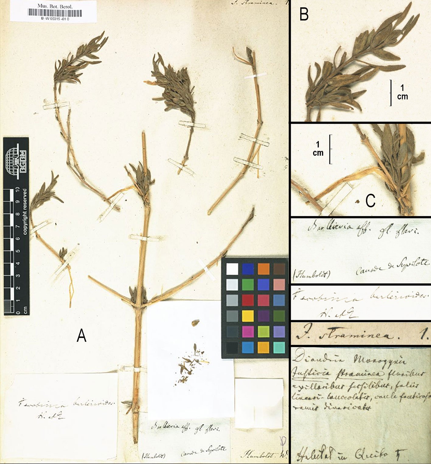
Figure 3. Tetramerium barlerioides, holotype (A. von Humboldt s.n.). A, Specimen at B-W; Curators Herbarium B (2000+); B, close-up of terminal foliose spike; C, partially folded corolla. Annotations noting (from top): affinities with Barleria, yellow flowers, collector (Humboldt), and collection locality (“Canada de Supilote”); Nees’ annotation (Jacobinia barlerioides); a subsequent determination (Justicia straminea); and on the backside, a brief description of the plant as J. straminea noting “Habitat in Quito.”
Description. Daniel (1986, as T. ochoterenae).
Distribution. Endemic to the DBBP in Mexico (Guerrero, Morelos, Puebla). Plants in the DBBP occur from northwestern Guerrero through central and northern Guerrero and Morelos to central and southern Puebla.
Flowering in DBBP. January-May.
Biotic communities in DBBP. Tropical deciduous forest and tropical deciduous forest/oak forest ecotone at 600-1,600 m elevation.
Voucher by state. Guerrero: Municipio de Zumpango del Río [= Eduardo Neri], Cañón del Zopilote, MEX 95, 3.3 km N de la desviación a Xochipala (17°49’31” N, 099°33’48” W), V. Steinmann & J. Porter 4921 (CAS, MEXU). Morelos: 6 km al NW de Jonacatepec, [ca. 18°50’54.96” N, 098°59’44.57” W], L. González Q. 3631 (DS, ENCB, MICH, MSC). Puebla: along Hwy. 190 between Oaxaca and Izúcar de Matamoros, NW of Tehuitzingo, 11 mi NW of Río Atoyac (18°27’N, 98°22’W), T. Croat & D. Hannon 65721 (CAS, MEXU).
Remarks. This species was known to Daniel (1986) from only 6 collections. Recent collecting has resulted in at least 31 total collections (Fig. 1), but the species remains known only from the DBBP. Updated information on phenology, habitat, and elevation is indicated above. The total distribution of the species (EOO) is 21,037.792 km2 and the AOO is 116 km2. If sufficient information concerning actual or potential threats (and locations) to this species were known, it could potentially be assessed as Endangered (EN) based on the AOO.
Nees (1847) indicated that Jacobinia barlerioides Nees was collected by Alexander von Humboldt “ad Canade de Supulote in districtu Quitensi.” As a result, the locality of Humboldt’s type collection has been attributed to Ecuador in various sources (e.g., IPNI, 2024; JSTOR, 2024). However, the species does not occur there, and no such locality is noted by Sandwith (1926) among Humboldt’s Ecuadorian collecting sites. However, “Cañada de Sopilote” and “Valle de Sopilote” are specifically listed among Humboldt and Bonpland’s Mexican collection localities by Sprague (1924). Indeed, the species has been collected numerous times in and near the Cañón del Zopilote in the DBBP of central Guerrero between Zumpango del Río and Mezcala. The canyon lies along the route between Chilpancingo and Taxco that Humboldt followed on his journey from Acapulco to Mexico City. He would have passed through the canyon in early April of 1803 (Stevens-Middleton, 1956).
Humboldt’s type specimen in the Willdenow Herbarium at B (Fig. 3) contains several annotations: “Barleria aff.,” “Jacobinia barlerioides” in Nees’ handwriting, and “J. straminea” (an unpublished name written on the sheet and cited in Nees’ protologue). In the protologue of Jacobinia barlerioides, Nees (1847) noted numerous characteristics that match those of Mexican plants treated as Tetramerium ochoterenae for the past ca. 4 decades (e.g., yellow corollas). However, he provided measurements of the corolla (“3/4 poll. longa” = ca. 25 mm) and capsule (“4 lin. longa” = ca. 8.4 mm) that would suggest instead the yellow-flowered form of the similar species, T. rubrum. Measurements made from a high-resolution color image of the type specimen reveal: the single intact corolla appears to be ca. 50 mm long, lobes of the lower lip of the corolla are linear and ca. 1.3 mm wide, and a capsule is ca. 11 mm long. These updated measurements and the geographic locality all conform to data for T. ochoterenae rather than T. rubrum (Daniel, 1986; see key to species above). Miranda (1941) described this species from Mexico as Anisacanthus ochoterenae. It was transferred to Tetramerium by Daniel (1986), who noted its morphological affinities with that genus, despite having elongate corollas with recurved, linear lobes and prominently protruding stamens and style (Fig. 2M) that more closely resemble flowers of Anisacanthus. Subsequent molecular phylogenetic data confirmed its generic status in Tetramerium (Daniel et al., 2008; McDade et al., 2018). Resemblance of flowers between species of Anisacanthus and this sole species of Tetramerium likely results from adaptations to similar hummingbird pollinators.
3. Tetramerium butterwickianum T.F. Daniel
Description. Daniel (1986).
Distribution. Endemic to the DBBP in Mexico. Plants occur in south-central to southeastern Michoacán.
Flowering in DBBP. November-March.
Biotic communities in DBBP. Thornscrub and tropical deciduous forest at 225-500 m elevation.
Voucher by state. Michoacán: Municipio de La Huacana, 1.5 km NE de Los Ranchos, ladera NW de Cerro El Barril (18°42’40” N, 102°00’15” W), V. Steinmann 4196 (CAS, IEB, MEXU).
Remarks. This species, previously known only from the type (Daniel, 1986), is now known from at least 6 collections. Conspicuous variation in the presence and/or densities of glandular trichomes on young stems, leaves, and inflorescence rachises are evident among them. The species total distribution (EOO) is 249.120 km2 and the AOO is 24 km2. If sufficient information concerning actual or potential threats (and locations) to this species were known, it could potentially be assessed as Endangered (EN) based on either the EOO or the AOO.
4. Tetramerium cruzii T.F. Daniel, sp. nov. Type. Mexico. Guerrero: Municipio de Arcelia, Campo Morado, Campamento Minero, 4.57 km W (18°11’45” N, 100°10’48” W), 1,177 m, bosque tropical caducifolio, 30-IV-2010 (flr, frt), R. Cruz 8344 (holotype: FCME 129144) (Fig. 4).
This species is distinctive in the genus by the combination of its elongate spikes 12-14 mm wide near midpoint; bracts that taper distally from or below the midpoint, have the apical portion neither twisted nor reflexed, and bear marginal trichomes to 1 mm long; white and pseudopapilionaceous corollas 15 mm long; and pubescent capsules.
Perennial herbs to 5 dm tall. Young stems subterete to subquadrate, 2-fariously pubescent with mostly retrorse eglandular trichomes to 0.1 mm long and often with erect stipitate glandular trichomes near distal nodes, older stems with epidermis exfoliating in strips. Leaves not seen. Inflorescences of terminal, sessile to pedunculate dichasiate spikes to 100 mm long (including peduncle, if present), 12-14 mm wide (excluding flowers) near midspike, spikes more or less dense (median internodes 4-5 mm long), peduncles (if present) to 12 mm long, peduncles and rachis evenly pubescent with erect subglandular, eglandular, and glandular trichomes < 0.1-0.2 mm long, dichasia opposite, decussate, sessile, 1-2 (or more?)-flowered. Bracts lance-ovate to ovate to elliptic, 9-12 mm long, (2-) 2.2-4 mm wide, 2.9-4.1 (-4.5) times longer than wide, proximally tapered, distally acuminate to attenuate, erect, not twisted, apically mucronate, mucro to 1 mm long, abaxial surface prominently (1 or) 3-veined, pubescent like rachis, margin ciliate with erect to flexuose eglandular trichomes to 1 mm long and erect to flexuose stipitate glandular trichomes 0.1-0.3 mm long. Bracteoles fused at base for ca. 0.5 mm, lance-linear to lanceolate, 7-9.5 mm long, 0.6-1.1 mm wide, abaxially pubescent with mostly erect eglandular trichomes 0.05-0.2 mm long and scattered stipitate glandular trichomes to 0.2 mm long, distally attenuate, apically subspinose, margin ciliate with flexuose eglandular trichomes to 0.7 mm long; secondary bracteoles (if present) smaller than bracteoles. Flowers sessile. Calyces 5-lobed, 2.5-3.5 mm long, tube 0.5 mm long, lobes subulate, 2-3 mm long, 0.2-0.3 mm wide, abaxially and marginally puberulent with a mixture of subglandular, stipitate glandular, and eglandular trichomes 0.01-0.1 mm long. Corollas pseudopapilionaceous, white with purplish markings on upper lip, 15 mm long, externally glabrous, tube 5 mm long, 1.8 mm in diam. at apex, narrow proximal portion 2.5 mm long, expanded throat 2.5 mm long, upper lip spatulate, 9 mm long, 4 mm wide, lower lip 10 mm long, lateral lobes obovate, 9 mm long, 5 mm wide, lower-central lobe conduplicate, ca. 6.5-7 mm long, 4.5 mm wide (spread open). Stamens ca. 7-7.5 mm long, thecae dark purple-maroon, 1.5 mm long. Pollen not observed. Styles 11 mm long, glabrous, stigmas 0.1 mm long, lobes not evident. Capsules 6-7.5 mm long, externally pubescent with erect to downward pointing eglandular trichomes to 0.1 mm long, stipe 1.8-2.5 mm long, head ovoid to ellipsoid, 4-5 mm long. Seeds 4, more or less plano-convex, 1.6-1.7 mm long, 1.5-1.7 mm wide, surfaces and margin minutely papillose and covered with more or less broad conical projections.
Distribution. Endemic to the DBBP in Mexico. Plants are known only from north-central Guerrero.
Flowering in DBBP. April.
Biotic community in DBBP. Tropical deciduous forest at 1177 meters elevation.
Conservation. Because the species is known solely by the type collection with no information on its current status or possible threats, a preliminary conservation assessment of Data Deficient (DD) concurs with IUCN (2022) guidelines.
Remarks. This species is named for Ramiro Cruz Durán, botanist at FCME, collector of the type and many other taxa from Guerrero, and helpful colleague. Guerrero is the second richest Mexican state for species of Tetramerium, with 10 species currently known to occur there (those listed herein plus T. guerrerense T.F. Daniel, which occurs in west-central Guerrero on the southwestern escarpment of the Sierra Madre del Sur and the adjacent coastal plain; Daniel 1986).
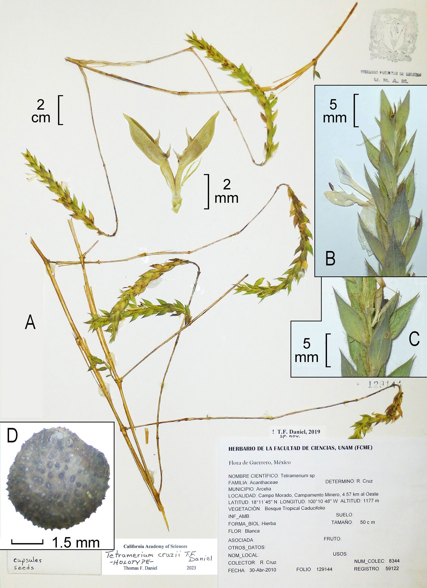
Figure 4. Tetramerium cruzii, holotype (Cruz 8344). A, Specimen at FCME; B, close-up of inflorescence with flower; C, close-up of inflorescence with capsule; D, close-up of seed.
5. Tetramerium emilyanum T.F. Daniel
Description. Daniel (1986).
Distribution. Endemic to the DBBP in Mexico. Plants occur in southeastern Michoacán.
Flowering in DBBP. November-December, March.
Biotic communities in DBBP. Tropical deciduous forest, tropical subdeciduous forest, and lower limit of oak zone at 550-630 m elevation.
Voucher by state. Michoacán: Municipio de Lázaro Cárdenas, carr. Nueva Italia-Playa Azul, 34 km S de Arteaga, [ca. 18°10’39.74” N, 102°16’30.71” W], J. Soto Núñez & S. Aureoles C. 7780 (IEB).
Remarks. This species is known definitively from only 2 collections from the same region of Michoacán. Plants intermediate between T. emilyanum and T. nervosum, potentially representing hybrids, were discussed by Daniel (1986). Additional recent collections intermediate between these species from the same region of southeastern Michoacán include Daniel 5316 (CAS) and Steinmann & Carranza 2165 (CAS).
6. Tetramerium glandulosum Oerst.
Description. Daniel (1986).
Distribution. Endemic to western and southern Mexico (Baja California Sur, Chihuahua, Colima, Durango, Guerrero, Jalisco, México, Michoacán, Morelos, Oaxaca, Puebla, Sinaloa, Sonora, Zacatecas). Plants in the DBBP occur from southwestern to northeastern Michoacán eastward through southern México, the northern half of Guerrero, and Morelos to central and southern Puebla and northwestern Oaxaca.
Flowering in DBBP. November-April
Biotic communities in DBBP. Thornscrub, tropical deciduous forest, tropical subdeciduous forest, and oak forest at 700-2,100 m elevation.
Voucher by state. Guerrero: 15.9 mi N of Zumpango del Río in Cañón del Zopilote, [ca. 17°49’46.30” N, 099°33’50.02” W], W. Anderson & C. Laskowski 4321 (MICH). México: Municipio de Ixtapan de la Sal, near Hwy. 55 between El Salitre and Ixtapan de la Sal (18°49’58.83” N, 099°40’2.96” W), D. Denham 3210 (CODAGEM). Michoacán: Municipio de Churumuco, El Limón, Ejido Llano Ojo de Agua (18°43’51” N, 101°40’23” W), M. Rojas 779 (MEXU). Morelos: Municipio de Puente de Ixtla, 6 km SE de Tilzapotla, camino a El Salto o 7 km de El Salto camino a Tilzapotla (18°28’06” N, 099°16’18” W, R. Ramírez et al. 2995 (MEXU). Oaxaca: La Reforma, 20 km NW de Tamazulapan (17°44’N, 097°44’W), A. García M. et al. 2058 (MEXU). Puebla: Municipio de Acatlán de Osorio, Barranca El Terrero, llegando por La Trinidad (18°12’41.30” N, 098° 0’46.91” W), C. Rojas-Martínez et al. 45 (MEXU).
Remarks. Tetramerium glandulosum is known from many collections throughout the DBBP. The collection cited above from the State of México represents the first report of the species in that state. It is the only species of Tetramerium in the DBBP with relatively large and pseudopapilionaceous corollas that are yellow (more intensely yellow and/or larger than in any of the cream to yellowish forms of T. nervosum or T. tenuissimum), and usually with 2 elongate reddish bands on the upper lip. It also differs from other species with white or cream to yellowish pseudopapilionaceous corollas by its habit (fragrant and viscid shrub to 3 m tall vs. non-fragrant perennial herbs to shrubs to 1 m tall).
7. Tetramerium glutinosum Lindau
Description. Daniel (1986).
Distribution. Endemic to the DBBP in Mexico. Plants occur from eastern Michoacán and southwestern México through Morelos and the northern half of Guerrero to western and south-central Puebla.
Flowering in DBBP. December-July.
Biotic communities in DBBP. Thornscrub, tropical deciduous forest, and ecotone between tropical deciduous and oak forests at 280-1,680 m elevation.
Voucher by state. Guerrero: Municipio de General Canuto Neri (Acapetlahuaya), ca. 4 km NE de El Crustel y 19 km NE de Arcelia, carr. Cd. Altamirano-Iguala (18°23’09.5” N, 100°07’43.5” W), J. Soto N. 21320 (IEB, MEXU). México: 25 km S de Amatepec, terraceria Amatepec-Arcelia, [ca. 18°31’38.28” N, 100°13’37.39” W], G. Flores F. & L. Terpán A. 745 (MEXU). Michoacán: Municipio de Huetamo, sobre Mex. 51, 7 km S de Huetamo (18°34’22” N, 100°51’51” W), V. Steinmann et al. 4116 (CAS, IEB, MEXU, XAL). Morelos: Municipio de Yautepec, Cañón de Lobos, 12-14 km E de Cuernavaca, carretera (libre) Cuernavaca-Cuautla, [ca. 18°51’31.93” N, 099°07’01.89” W], S. Koch & J. García P. 7649 (MEXU). Puebla: 5 mi W of Matamoros, [ca. 18°34’07.62” N, 098°32’53.22” W], D. Dunn & D. Dunn 18755 (ENCB, MSC, NY).
Remarks. Daniel (1986) cited 11 collections of this species. At least 47 collections are now known from throughout its total geographic range in the DBBP. The total geographic distribution of the species (EOO) is 34,092.476 km2 and the AOO is 164 km2. If sufficient information concerning actual or potential threats (and locations) to this species were known, it could potentially be assessed as Endangered (EN) based on the AOO.
Tetramerium glutinosum is a fragrant and more or less viscid perennial herb to shrub to 1 m tall. It is the only species of the genus in the DBBP with purple flowers. The conspicuous mucro at the bracteal apex is often conspicuously curved, bent, or coiled. Floral visits by a megachilid bee (Dianthidium sp.) were noted by Daniel (1986).
8. Tetramerium langlassei G.B. Happ
Description. Daniel (1986).
Distribution. Southern Mexico (Guerrero, Jalisco, Michoacán, Veracruz). In the DBBP, plants occur from western to eastern Michoacán and southward into western Guerrero.
Flowering in DBBP. November-February, May
Biotic communities in DBBP. Tropical deciduous forest and ecotone between tropical deciduous forest and oak forest at 302-1,450 meters elevation.
Voucher by state. Guerrero: Municipio de Coahuayutla de Guerrero, 1.5 km N de La Vainilla (18°14’53.5” N, 101°30’30.4” W), J. Calónico Soto 13457 (MEXU). Michoacán: Municipio de La Huacana, E foothills of Sierra Las Cruces, 3.5 km (air) SW of Los Ranchos, trail to La Verdura (ca. 18°41’00” N, 102°02’45” W), V. Steinmann 3180 (CAS, IEB).
Remarks. Daniel (1986) cited 11 collections of this species; at least 20 collections are currently known.
9. Tetramerium michoacanum T.F. Daniel, sp. nov. Type. Mexico. Michoacán: Municipio de Churumuco, La Barranca, Ejido Llano Ojo de Agua (18°42’11” N, 101°40’20” W), 365 m, bosque tropical caducifolio, 24-IV-2016 (flr), M. Rojas 735 (holotype: MEXU, accession 1499906!). (Fig. 5).
Tetramerium michoacanum differs from T. nervosum by its inflorescence rachis and bracteal margins with more or less densely floccose (vs. neither dense nor floccose) trichomes, distally apically attenuate (vs. rounded to acute to acuminate) bracts, longer (10-13 vs. 1.5-10 mm) bracteoles, generally longer (23-29 vs. 10-23 mm) corollas, and longer (2-3 vs. 0.9-1.7 mm) anther thecae.
Perennial herbs or shrub to 1 m tall. Young stems subquadrate to 2-sulcate, 2-fariously pubescent with retrorse (to flexuose, especially at nodes) eglandular trichomes 0.2-0.7 mm long, older stems with epidermis exfoliating in strips. Leaves petiolate, petioles 3-21 mm long, pubescent with straight to flexuose eglandular trichomes, blades lance-ovate, to ovate, 18-83 mm long, 5-29 mm wide, 2.3-5.5 (-8.3) times longer than wide, acuminate to attenuate at apex, rounded to acute to subattenuate at base, adaxial surface pubescent with erect to antrorse to antrorsely appressed eglandular trichomes 0.05-0.3 mm long, abaxial surface more or less evenly pubescent with flexuose to retrorse to antrorse eglandular trichomes 0.1-0.3 mm long, margin ciliate with mostly antrorse eglandular trichomes to 0.5 mm long. Inflorescences of terminal, sessile to short-pedunculate dichasiate spikes to 75 mm long (including peduncle) and 9-12 mm wide (excluding flowers) near midspike, spikes more or less dense (median internodes 4-6 mm long), peduncles (if present) to 2 mm long, densely and evenly pubescent with flexuose to mostly straight and downward pointing eglandular trichomes to 0.8 mm long, rachis more or less densely and more or less 2-fariously pubescent with flexuose and largely interwoven eglandular trichomes to 1.5 mm long (appearing more or less floccose), dichasia opposite, decussate, sessile, 1-2 (or more?)-flowered. Bracts lance-ovate to narrowly ovate-elliptic, 11-16 mm long, 3-5 mm wide, 2.8-4.7 times longer than wide, proximally slightly tapered and truncate at base, distally attenuate, erect to slightly recurved, straight or slightly twisted, apically mucronate, mucro 0.1-0.3 mm long, abaxial surface prominently 3-veined, proximal bracts abaxially pubescent with an understory of subglandular and stipitate glandular trichomes 0.02-0.2 mm long and an overstory of more or less interwoven eglandular trichomes to 0.5 mm long, distal bracts less densely pubescent with a similar understory and an overstory of flexuose eglandular trichomes to 1 mm long (especially along veins), margin of bracts ciliate with subglandular and glandular trichomes to 0.5 mm long and flexuose eglandular trichomes to 2 mm long, eglandular marginal trichomes becoming cotton-like and so dense as to obscure rachis, bracteoles, and calyces. Bracteoles linear-lanceolate, 10-13.5 mm long, 0.8-1.5 mm wide, abaxially pubescent with flexuose trichomes to 2.5 mm long, apically acute, emucronate, margin ciliate like bracts but with trichomes sparser. Flowers sessile. Calyces 5-lobed, 4.5-6.5 mm long, tube 0.5-1 mm long, lobes subulate, subequal in size, 3.5-6 mm long, 0.3-0.4 mm wide, abaxially and marginally pubescent with an understory of erect eglandular and subglandular to glandular trichomes 0.01-0.02 (-0.05) mm long and an overstory of sparse flexuose eglandular trichomes to 1 mm long. Corollas pseudopapilionaceous, white with upper lip cream bearing a purplish chevron outlined with maroon, (21-) 23-29 mm long, externally glabrous, tube subcylindric, 12-16 mm long, 1.7-2.2 mm in diam. at apex, narrow proximal portion 8-11 mm long, more or less expanded throat 2-5 mm long, upper lip obovate to subspatulate, 11-14.6 mm long, 3.5-4 mm wide, lower lip 13.5-15 mm long, lateral lobes elliptic to obovate-elliptic, 12-13 mm long, 6.5-10 mm wide, lower-central lobe conduplicate, 8-12 mm long, 4.4-6 mm wide (spread open). Stamens 7.5-13 mm long, thecae 2-3 mm long. Pollen euprolate, polar diameter (P) 46-53 µm, equatorial diameter (E) 28-33 µm, P:E = 1.4-1.8. Styles 19-20 mm long, glabrous distally and sometimes with a few eglandular trichomes proximally, stigmas 0.2-0.3 mm long, lobes not evident, ovary glabrous. Capsules and seeds not seen.
Distribution. Endemic to the DBBP in Mexico. Plants occur in the northern watershed of the Río Atoyac in the Cerro Conchitero region of southeastern Michoacán.
Flowering in DBBP. November-December, April.
Biotic communities in DBBP. Tropical deciduous forest at 365-664 meters elevation.
Conservation. The species is known only from 3 collections. The known distribution of T. michoacanum consists of an EOO of 46.592 km2 and the AOO is 12 km2. Additional information on actual or potential threats (and locations) would be useful to make a potential conservation assessment.
Paratypes. Mexico. Michoacán: Municipio de Churumuco, Cerro El Zipimo, ca. 3.7 km (línea recta) NW del Ejido Llano de Ojo de Agua (18°42’22” N, 101°40’18” W), 530 m, 15-IX-2023 (flr), G. Ibarra Manríquez et al. 7326 (IEB, MEXU); Municipio de Churumuco, Las Higueras, Ejido Llano Ojo de Agua (18°43’36” N, 101°39’58” W), 664 m, 13-XI-2014 (flr), M. Rojas 283 (MEXU). Additional duplicate specimens to be distributed.
Remarks. The species is named for the Mexican state from which all plants of it known to date have originated. Michoacán is the richest Mexican state for species of Tetramerium, with 13 species currently known to occur there (those listed herein plus T. diffusum Rose and T. rzedowskii T.F. Daniel, both of which occur just to the west and northwest of the DBBP). Capsules and seeds were not available for measurements for T. michoacanum. The presence or absence of eglandular trichomes on capsules in species of Tetramerium is a diagnostic character for all species except T. nervosum, in which both states occur. It is possible that capsules of T. michoacanum are glabrous because ovaries seen lack trichomes. However, some species with pubescent capsules (e.g., T. tenuissimum and perhaps others) have the younger ovaries glabrous and the older ones pubescent. Thus, capsule pubescence of T. michoacanum remains to be determined. The euprolate pollen of T. michoacanum is typical for the genus (e.g., Daniel, 1986, 1998) and shows harmomegathic variation that affect its shape (Fig. 6).
The distinctions noted in the key above distinguish T. michoacanum from morphologically similar and/or geographically close congeners. It also shares some morphological traits (e.g., dense and elongate trichomes in the inflorescence, especially along the bracteal margins) with T. tetramerioides (Lindau) T.F. Daniel from a region of tropical deciduous forest in southeastern Oaxaca. Tetramerium tetramerioides differs from T. michoacanum by: young stems with an understory of glandular trichomes 0.05-0.2 mm long; spikes 3-7 mm wide near midpoint; bracts linear-lanceolate to lanceolate-elliptic, 7-10 × 1-2.5 mm, and usually with only the midvein evident; bracteoles 6-8 × 0.5-0.8 mm; calyces 3.2-4 mm long; and corollas 14-15 mm long. Although duplicates are noted on the specimen labels of all 3 known collections cited above, the destinations of most of those duplicates remain unconfirmed at present.
10. Tetramerium nervosum Nees
Description. Daniel (1986).
Distribution. USA, Mexico (Aguascalientes, Baja California Sur, Campeche, Chiapas, Chihuahua, Coahuila, Colima, Durango, Guanajuato, Guerrero, Hidalgo, Jalisco, México, Michoacán, Morelos, Nayarit, Nuevo León, Oaxaca, Puebla, Querétaro, Quintana Roo, San Luis Potosí, Sinaloa, Sonora, Tamaulipas, Veracruz, Yucatán, Zacatecas), Guatemala, El Salvador, Honduras, Nicaragua, Costa Rica, Panama, Colombia, Venezuela, Ecuador, and Peru. Plants occur throughout most of the DBBP (from southeastern Jalisco through Michoacán, southern México, northern and central Guerrero, and Morelos to south-central Puebla and northwestern Oaxaca). It has not been recorded from portions of the states of Ciudad de México, Tlaxcala, and Veracruz that are sometimes included in delimitations of the DBBP.
Flowering in DBBP. September-May.
Biotic communities in DBBP. Thornscrub, tropical deciduous forest, tropical deciduous forest-oak forest ecotone, oak forest, tropical deciduous forest-pine-oak ecotone, pine-oak forest at 200-1,940 meters elevation.
Voucher by state. Guerrero: Municipio de Teloloapan, Tehuixtla (18°18’16.8” N, 099°55’34.3” W), D. Tejero-Díez & A. Torres 6466 (MEXU). Jalisco: Municipio de Jilotlán de los Dolores, 7 km SE de Huapala, camino a Jilotlán, [ca. 19°20’33.93” N, 103°05’08.41” W], A. Mendoza et al. 3700 (MEXU). México: Municipio de Tejupilco, ca. 2 km NO del centro de Tejupilco, camino a San José de La Laguna, en la col. Vista Bella (18°54’46.1” N, 100°09’26.5” W), J. Soto N. 21287 (MEXU). Michoacán: Municipio de Carácuaro, camino de La Eréndira a El Puerto del Salitrillo, ca. 2 km E del entronque con la carr. La Eréndira-Caracuáro (18°50’29.50” N, 100°55’37.19” W), J. Soto N. & B. Gómez Rosales 17372 (MEXU). Morelos: Municipio de Tepalcingo, 4 km SW de El Limón (18°30’00” N, 098°57’28” W), A. Ramírez Guadarrama et al. 789 (MEXU). Oaxaca: Dto. Huajuapan, Cañada Cuasá, 3 km (línea recta) N de San Juan Bautista Suchitepec (17°59’57.3” N, 097°39’10.5” W), R. Redonda Martínez et al. 460 (MEXU). Puebla: Municipio de Acatlán de Osorio, Barranca La Macahuite (18°12’41.32” N, 098°00’46.91” W), C. Rojas-Martínez et al. 49 (MEXU).
Remarks. This is the most widely distributed and morphologically diverse species in the genus (Daniel 1986). It is distributed from the southwestern USA to northwestern Peru. Plants in the DBBP show morphological variation in calyx lobe number (4 or 5), bract shape (lance-ovate to ovate to elliptic to subcircular), corolla color (white to pale yellow), pubescence (length, form, and glandular vs. eglandular trichomes), and patterning of discolorations on the upper lip (Fig. 2K, L). Daniel (1986) noted visitation to flowers of T. nervosum by several genera of bombyliid flies and a genus of hesperiid butterflies.

Figure 5. Tetramerium michoacanum. A, Holotype at MEXU (Rojas 735); B, live plant with leaves and flowering inflorescence (Ibarra Manríquez et al. 7326); C, live flower (frontal view; Ibarra Manríquez et al. 7326); D, live flower (side view; Ibarra Manríquez et al. 7326); E, portion of inflorescence with flower showing dense, floccose pubescence concealing rachis (from holotype); F, bracteole (from holotype). Photos B-D by G. Ibarra-Manríquez.
11. Tetramerium pauciflorum T.F. Daniel & V.W. Steinm.
Description. Daniel and Steinmann (2016).
Distribution. Endemic to the DBBP in Mexico. The species has a restricted distribution in southeastern Michoacán. Daniel and Steinmann (2016) noted that it is known from 2 regions ca. 30 km apart, the valleys of the Río Marquez to the north and the Río Tepalcatepec to the south.
Flowering in DBBP. November, February, May.
Biotic community in DBBP. Tropical deciduous forest at 250-400 meters elevation.
Conservation. The 5 known collections from 4 localities reveal an extent of occurrence (EOO) of ca. 3 km2 and an area of occupancy (AOO) of 8 km2. Despite the limited distribution, Daniel and Steinmann (2016) provided a rationale for a provisional conservation assessment of Least Concern (LC) for this species. Additional information on actual or potential threats (and locations) would be useful to make a potential conservation assessment.
Voucher by state. Michoacán: Municipio de Múgica, 5.5 km NE de la salida a Nueva Italia sobre la autopista Morelia-Lázaro Cárdenas (19°01’57” N, 102°03’12” W), V. Steinmann & Y. Ramírez-Amezcua 8089 (CAS, MEXU,RSA).
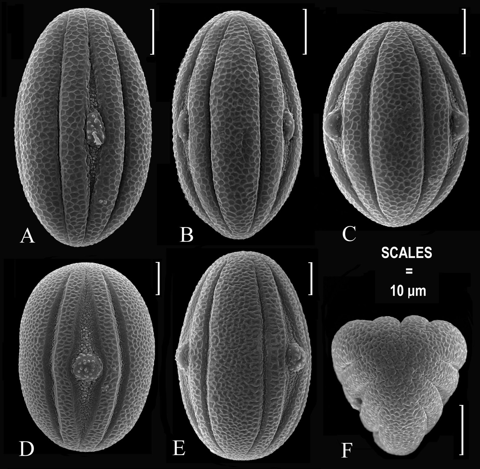
Figure 6. Pollen of Tetramerium michoacanum (Rojas 735, A-C) and T. barlerioides (D-F). A, Apertural view; B, interapertural view; C, interapertural view (showing harmomegathic variation); D, apertural view (Steinmann & Porter 4921); E, interapertural view (Steinmann & Porter 4921); F, polar view (Grimes et al. 2612).
12. Tetramerium rubrum G.B. Happ
Description. Daniel (1986).
Distribution. Endemic to west-central Mexico (Guerrero, Jalisco, México, Michoacán, Nayarit). Plants occur throughout much of the DBBP: western Jalisco, southern and northeastern Michoacán, western Guerrero, western México, and southwestern Puebla. It appears to be most abundant in Michoacán and western México. No collections have been seen from Morelos, central and eastern Guerrero, or Oaxaca.
Flowering in DBBP. November-June.
Biotic communities in DBBP. Tropical deciduous forest, oak forest, and pine-oak forest at 200-1,700 meters elevation.
Voucher by state. Guerrero: Municipio de La Unión, MEX 134, ca. 31 km NE de Vallecitos y 3 km E de Puerto del Bálsamo (17°58’49” N, 101°12’16” W), V. Steinmann & J. Porter 4932 (CAS, MEXU). Jalisco: Municipio de de Jilotlán de los Dolores, 5 km al N de Tepalcatepec, [ca. 19°13’33.74” N, 102°52’04.83” W], J. Rzedowski 16639 (ENCB). Mexico: Municipio de Santo Tomás de los Plátanos, valley just N of (below) Nuevo Santo Tomás (19°11’05.37” N, 100°15’55.93” W), T. Daniel et al. 12323 (CAS). Michoacán: Municipio de Buenavista Tomatlán, ca. 3 km SW de El Terrero, [ca. 19°02’34.91” N, 102°40’24.62” W], J. Soto Núñez et al. 8045
(CAS,MEXU).
Remarks. The very similar species T. abditum and T. rubrum both occur in Nayarit and Michoacán (and likely Jalisco, but T. abditum has not been recorded from that state, which lies between the other 2), and maintain their distinctions as noted in the key. Plants of T. rubrum with yellow corollas appear almost as frequently as those with red flowers. Collections with yellow corollas are known from Guerrero (Campos R. 360, MEXU; Moreno Gtz. & Alberto Monroy 742, MEXU) and Michoacán (Daniel & Butterwick 3270, ASU, CAS, ENCB, MEXU, MICH, NY; Rojas 704 and 780, MEXU; Roman de Soto N. et al. 8045, CAS; Steinmann 5065, CAS; Steinmann et al. 3997, CAS).
13. Tetramerium tenuissimum Rose
Description. Daniel (1986).
Distribution. Western and southern Mexico (Campeche, Chiapas, Chihuahua, Colima, Guanajuato, Guerrero, Jalisco, México, Michoacán, Morelos, Nayarit, Oaxaca, Sinaloa, Sonora, Veracruz, Yucatán, Zacatecas), Guatemala, and El Salvador. In the DBBP this species is widespread, occurring from eastern Michoacán and western México through northern and central Guerrero and Morelos to the borders of Puebla and Oaxaca. It likely occurs within the latter 2 states as well, but no collections from them have been seen.
Flowering in DBBP. October-April.
Biotic communities in DBBP. Tropical deciduous forest and oak forest at 280-1,500 meters elevation.
Voucher by state. Guerrero: Municipio de Taxco, 4 km SW del crucero Cacahuamilpa-Toluca, camino a Taxco, [ca. 18°34’20.01” N, 099°34’5.89” W], E. Martínez S. & E. Cabrera 73 (MEXU). México: Municipio de Santo Tomás de los Plátanos, valley just N of (below) Nuevo Santo Tomás (19°11’05.37” N, 100°15’55.93” W), T. Daniel et al. 12328 (CAS). Michoacán: Municipio de Huetamo, MEX 51, 7 km S de Huetamo (18°34’22” N, 100°51’51” W), V. Steinmann et al. 4117 (CAS, MEXU). Morelos: Municipio de Jonacatepec, 2 km S de Tlayca, [ca. 18°41’28.43” N, 098°51’54.72” W], E. Cabrera C. et al. 12137 (MEXU).
Remarks. Tetramerium tenuissimum is newly documented from the state of México. Daniel (1986) noted visitation to flowers of this species by bombyliid flies. Plants are sometimes confused with T. nervosum. These species can be distinguished by the characters in the following couplet:
1a. Bracts with margins conspicuously and more or less densely ciliate with trichomes to 3.5 mm long, at least some (usually most) of the trichomes ≥ 1 mm long, abaxially more or less palmately and prominently 3 or 5 (or 7)-veined, apically usually more or less recurved and partially twisted; corolla tube 5-12 mm long T. nervosum
1b. Bracts with margins inconspicuously and more or less sparsely ciliate with trichomes to 0.5 mm long, abaxially more or less palmately and often obscurely (1 or) 3-veined, apically erect and not twisted; corolla tube (2.5-) 3-5 mm long T. tenuissimum
14. Tetramerium vargasiae T.F. Daniel & R. Cruz Durán
Description. Daniel and Cruz Durán (2016).
Distribution. Endemic to the DBBP in Mexico. Plants occur in north-central Guerrero.
Flowering in DBBP. March.
Biotic community in DBBP. Tropical deciduous forest at 650 meters elevation.
Conservation. Because the species is known solely by the type collection with no information on its current status or possible threats, a preliminary conservation assessment of Data Deficient (DD) concurs with IUCN (2022) guidelines.
Voucher by state. Guerrero: Municipio de Huitzuco de los Figueroa, 0.7 km NE de San Francisco Ozomatlán [ca. 17°56’0.63” N, 099°19’37.41” W], A. Vargas P. 288 (FCME).
Acknowledgments
I thank the following persons for their assistance with obtaining materials: Guillermo Ibarra-Manríquez (UNAM-Pátzcuaro), Rosalinda Medina Lemos (MEXU), and Nancy Hensold (F). Photographers Dale Denham, Victor Steinmann, José Javier Barrios Flores, and Guillermo Ibarra-Manríquez generously made their images available. Jurai Paule (B) helped me obtain the image of Tetramerium barlerioides from the Willdenow Herbarium at B.
References
Arreguín-Sánchez, M., Fernández-Nava, R., & Guerrero-Ruiz, M. I. (2002). La familia Celastraceae en la cuenca del río Balsas, México. Polibotánica, 14, 1–50.
Comisión Nacional de Agua. (2011). D.F. México: Coordinación General de Atención Institucional, Comunicación y Cultura del Agua, Comisión Nacional del Agua.
Curators Herbarium B (2000+). Digital specimen images at the Herbarium Berolinense. [Dataset]. Version: 28 Feb 2024, image ID: 238195. Botanic Garden and Botanical Museum Berlin. Retrieved on January 10th, 2024 from: https://herbarium.bgbm.org/object/BW00315010
Daniel, T. F. (1986). Systematics of Tetramerium (Acanthaceae). Systematic Botany, Monographs, 12, 1–134. https://doi.org/
10.2307/25027628
Daniel, T. F. (1998). Pollen morphology of Mexican Acanthaceae: diversity and systematic significance. Proceedings of the California Academy of Sciences, 50, 217–256.
Daniel, T. F. (2003). New and reconsidered Mexican Acan-
thaceae X. Flora del Bajío region. Novon, 13, 37–48. https://doi.org/10.2307/3393563
Daniel, T. F., & Cruz Durán, R. (2016). Tetramerium vargasiae (Acanthaceae), a new species from the Basin of the Río Balsas in Guerrero, Mexico. Proceedings of the California Academy of Sciences, 63, 159–162.
Daniel, T. F., McDade, L. A., Manktelow, M., & Kiel, C. A. (2008). The “Tetramerium Lineage” (Acanthaceae: Acanthoideae: Justicieae): delimitation and infra-lineage relationships based on cp and nrITS sequence data. Systematic Botany, 33, 416–436. https://doi.org/10.1600/036364408784571581
Daniel, T. F., & Steinmann, V. M. (2016). Tetramerium pau-
ciflorum (Acanthaceae: Justicieae): a new species from the basin of the Río Balsas in Michoacán, Mexico. Proceedings of the California Academy of Sciences, 63, 567–573.
Flores-Tolentino, M., Beltrán-Rodríguez L., Morales-Linares J., Ramírez Rodríguez J. R., Ibarra-Manríquez G., Dorado, O. et al. (2021). Biogeographic regionalization by spatial and environmental components: Numerical proposal. Plos One, 16, e0253152. https://doi.org/10.1371/journal.pone.0253152
Flores-Tolentino, M., Ramírez-Rodríguez, J. R., Morales-Linares, J., Ibarra-Manríquez, G., Dorado, O., & Villaseñor, J. L. (2023). Delimitación geográfica y florística de la provincial fisiográfica de la Depresión del Balsas, México, con énfasis en el bosque tropical estacionalmente seco. Revista Mexicana de Biodiversidad, 94, e944985. https://doi.org/10.22201/ib.20078706e.2023.94.4985
GeoCAT. (2024). Geospatial Conservation Assessment Tool. Royal Botanic Gardens, Kew. Retrieved on February 14th, 2024 from: https://geocat.iucnredlist.org/
Google Earth Pro. (2023). Google Earth Pro, version 7.3.4.8248. Maps. Retrieved during May, 2023 from: https://sites.
google.com/earthoutreach.org/imw-australia/agenda/goo
gle-earth-pro
IPNI (International Plant Names Index). (2024). Database. The Royal Botanic Gardens, Kew. Retrieved on February 15th, 2024 from: http://www.ipni.org
IUCN (International Union for Conservation of Nature). (2022). Guidelines for using the IUCN Red List Categories and Criteria, version 15.1. Standards and Petitions Committee. Retrieved on 02 March, 2024 from: http://www.iucnredlist.org/documents/RedListGuidelines.pdf
JSTOR. (2024). JSTOR Global Plants. ITHAKA Database. Retrieved on February 14th, 2014 from: https://plants.jstor.org/
McDade, L. A., Kiel, C. A., & Daniel, T. F. (2018). The Tetra-
merium Lineage (Acanthaceae, Justicieae) revisited: phylogenetic relationships reveal polyphyly of many New World genera accompanied by rampant evolution of floral morphology. Systematic Botany, 43,97–116. https://doi.org/10.1600/036364418X697003
Miranda, F. (1941). Estudios sobre la vegetación de México. 1. La vegetación de los cerros al sur de la Meseta de Anáhuac El Cuajiotal. Anales del Instituto de Biología, Universidad Nacional Autónoma de México, 12, 569–614.
Nees von Esenbeck, C. G. (1847). Acanthaceae. In A. de Candolle (Ed.), Prodromus Systematis Naturalis Regni Vegetabilis, Vol. 1 (pp. 46–519). Paris: Victoris Masson.
Rzedowski, J. (1978). Vegetación de México. Ciudad de México: Limusa.
Sandwith, N. Y. (1926). XXIV. –Humboldt and Bonpland’s itinerary in Ecuador and Peru. Bulletin of Miscellaneous Information (Royal Botanic Gardens, Kew), 1926, 181–190.
Sprague, T. A. (1924). II. –Humboldt and Bonpland’s Mexican itinerary. Bulletin of Miscellaneous Information (Royal Botanic Gardens, Kew), 1924, 20–27.
Stevens-Middleton, R. L. (1956). La obra de Alexander von Humboldt en México, fundamento de la geografía moderna. Boletín de la Sociedad Mexicana de Geografía y Estadística, 81,1–269.
Thiers, B. M. (2024). Index Herbariorum. NYBG. https://sweetgum.nybg.org/science/ih/
Wikipedia (Wikipedia contributors). (2023). Balsas River. In Wikipedia, The free encyclopedia. Retrieved during December, 2023 from: https://en.wikipedia.org/w/index.php?title=Balsas_River&oldid=1181414412

Lista comentada de las hormigas (Hymenoptera: Formicidae)de Calvillo, Aguascalientes, México
Israel de Jesús Rodríguez-Elizalde * y Gabriela Castaño-Meneses
Universidad Nacional Autónoma de México, Campus Juriquilla, Facultad de Ciencias, Unidad Multidiscliplinaria de Docencia e Investigación, Laboratorio de Ecología de Artrópodos en Ambientes Extremos, Boulevard Juriquilla Núm. 3001, 76230 Juriquilla, Querétaro, México
*Autor para correspondencia: ijrodriguez.elizalde@gmail.com (I.J. Rodríguez-Elizalde)
Recibido: 29 febrero 2024; aceptado: 21 junio 2024
Resumen
La familia Formicidae constituye un grupo de himenópteros eusociales de gran diversidad taxonómica y funcional conocidos como hormigas. El estado de Aguascalientes es de los menos conocidos en cuanto a riqueza de hormigas en México. Por ello, el presente estudio pretende conocer la mirmecofauna del municipio de Calvillo, Aguascalientes, México. Se realizaron recolectas en 28 localidades, tanto de manera sistemática como no sistemática en diferentes tipos de vegetación: 11 en bosque de encino (8 perturbados), 4 en bosque tropical subcaducifolio bajo, 5 en matorral subtropical y 8 en agroecosistema. Se aplicaron 4 métodos de colecta: trampas de caída y arbóreas cebadas con miel y atún, cernidos de hojarasca procesados con embudo Berlesse, y colecta manual. Los ejemplares fueron conservados en alcohol, separados y determinados hasta la categoría taxonómica posible. Se elaboró una lista comentada de las especies colectadas. Se recolectaron 40,395 ejemplares pertenecientes a 56 especies, 31 géneros, 15 tribus y 6 subfamilias, siendo Myrmicinae la de mayor riqueza con 29 especies. Trece especies se registran por primera vez en el estado. Los resultados obtenidos evidencian que se requieren más estudios a fin de conocer aspectos biológicos, ecológicos y de distribución sobre la mirmecofauna de Aguascalientes.
Palabras clave: Mirmecofauna; Muestreo; Nuevos registros; Inventario; Riqueza de especies
© 2024 Universidad Nacional Autónoma de México, Instituto de Biología. Este es un artículo Open Access bajo la licencia CC BY-NC-ND
(http://creativecommons.org/licenses/by-nc-nd/4.0/).
Annotated checklist of ants (Hymenoptera: Formicidae) from Calvillo, Aguascalientes, Mexico
Abstract
The Formicidae family constitutes a group of eusocial hymenopterans of great taxonomic and functional diversity known as ants. The state of Aguascalientes is one of the least known in terms of ant richness in Mexico. Therefore, the present study aims to know the myrmecofauna (ants) of the municipality of Calvillo, Aguascalientes, Mexico, in order to increase the number of records in the state. Collections were made in a systematic and non-systematic manner: 11 in oak forest (8 disturbed), 4 in low subdeciduous tropical forest, 5 in subtropical shrubland and 8 in agroecosystem. Four collection methods were implemented: pitfall and tree traps baited with honey and tuna, leaf litter sifting that was processed with a Berlesse funnel, and manual collection. The specimens were preserved in alcohol, separated and determined to the possible taxonomic level. An annotated list of the collected species was prepared. A total of 40,395 specimens belonging to 56 species, 30 genera, 15 tribes and 6 subfamilies were collected, with Myrmicinae being the richest with 29 species. Thirteen species are recorded for the first time in the state. Results show that are necessary more studies to know biological, ecological and distribution aspects of the myrmecofauna of Aguascalientes.
Keywords: Myrmecofauna; Sampling; New records; Inventory; Species richness
Introducción
El orden Hymenoptera se considera un grupo hiperdiverso junto con Coleoptera, Lepdioptera y Diptera. Estudios recientes indican que probablemente se trate del orden de insectos más diverso en el mundo, incluso por encima de Coleoptera, debido al poco conocimiento en torno a las avispas parasitoides, altamente diversas, pero pobremente estudiadas (Forbes et al., 2018). Los insectos que pertenecen a este grupo (abejas, avispas y hormigas) presentan ojos compuestos normalmente bien desarrollados y aparato bucal estructuralmente masticador, aunque adaptado en algunos casos para lamer y succionar. Las alas son membranosas, con tendencia a la reducción de la venación; el primer par siempre es mayor que el segundo. El ovipositor en las hembras se encuentra modificado a modo de sierra en el suborden Symphyta, taladro en el suborden Parasitica o aguijón en el suborden Aculeata (Fernández-Gayubo y Pujade-Villar, 2015).
Las hormigas son un grupo de himenópteros sociales de gran diversidad taxonómica y funcional. Todas sus especies pertenecen a la familia Formicidae dentro de la superfamilia Vespoidea, la cual se cree constituye un grupo monofilético (Brothers y Carpenter, 1993). Se caracterizan por poseer antenas geniculadas con el escapo casi tan largo como el resto de los antenómeros; mandíbulas bien desarrolladas y mesosoma (tórax más segmento abdominal I) separado del gáster por 1 o 2 segmentos articulados, llamados peciolo y pospeciolo (Hölldobler y Wilson, 1990).
Son organismos eusociales, es decir, tienen una estructura social avanzada, en la cual individuos adultos de diferentes generaciones conviven en el mismo tiempo y espacio (sobrelapamiento de generaciones) y existe división de trabajo (Wilson y Hölldobler, 2005). Cada casta está adaptada morfológica, fisiológica y etológicamente para llevar a cabo una tarea en particular: las reinas y los machos (generalmente alados) cumplen la función reproductiva; mientras que las obreras (hembras estériles y ápteras) se encargan del resto de las tareas que tienen lugar dentro y fuera de la colonia (Hölldobler y Wilson, 1990).
Dentro de los artrópodos, las hormigas son uno de los grupos más diversos. Se sabe que en el mundo hay más de 14,000 especies vivas descritas pertenecientes a 342 géneros incluidos en 16 subfamilias (AntWeb, 2024). Para nuestro país se conocen 927 especies (Vásquez-Bolaños, 2015). Por su parte, Aguascalientes ocupa el séptimo lugar entre las entidades pobremente conocidas en cuanto a mirmecofauna (Vásquez-Bolaños y Escoto-Rocha, 2016). Entre los estudios que mencionan especies de hormigas presentes en este estado, se cuenta con el de Cañedo (1988), quien reporta 9 especies para el municipio de Aguascalientes, así como aspectos básicos sobre su biología y hábitos; Escoto-Rocha et al. (2001), llevaron a cabo una revisión del material de Hymenoptera depositado en la Colección Zoológica de la Universidad Autónoma de Aguascalientes (CZUAA), incluyendo 10 especies de Formicidae; Vásquez-Bolaños (2011), Ríos-Casanova (2014) y Vásquez-Bolaños (2015) reportan 9 especies; Rodríguez-Elizalde y Escoto-Rocha (2015), pusieron al día el listado de especies de Formicidae de la CZUAA con 17 especies para Aguascalientes; Vásquez-Bolaños y Escoto-Rocha (2016), actualizaron el listado de Formicidae para el estado, reconociendo 32 especies; más recientemente, González-Martínez y Vásquez-Bolaños (2019) documentaron 26 especies del cerro Juan El Grande, en el municipio El Llano; Rodríguez-Elizalde (2019) menciona 41 especies para el municipio de Calvillo, y finalmente 17 especies registran Dáttilo et al. (2020).
Con este trabajo se pretende conocer la mirmecofauna del municipio de Calvillo, en 28 localidades considerando la variedad del uso de suelo imperante en éste: bosque de encino (conservado y perturbado), bosque tropical subcaducifolio bajo, matorral subtropical y agroecosistema (cultivo de guayaba).
Materiales y métodos
Aguascalientes se localiza en la parte central de la República Mexicana con una superficie de 5,680.33 km2 (0.3% del país). Colinda al norte, este y oeste con Zacatecas, al sur y este con Jalisco. Cuenta con 11 municipios: Aguascalientes, Asientos, Calvillo, Cosío, Jesús María, Pabellón de Arteaga, Rincón de Romos, San José de Gracia, Tepezalá, San Francisco de los Romo y El Llano (Esparza-Juárez, 2008).
Calvillo se ubica al suroeste del estado, su superficie es de 908.22 km2 (Esparza-Juárez, 2008). Presenta sierra alta con mesetas, valle intermontano con lomeríos, meseta y lomeríos con cañadas (INEGI, 2008a). Los tipos de clima imperantes son semiseco semicálido, BS1hw(w), semiseco templado, BS1kw y templado subhúmedo con lluvia en verano, C(w0) (INEGI, 2008b). Se reconocen 9 tipos de vegetación, sin embargo, por su extensión, los más representativos son: bosque de encino y vegetación subtropical, representada por bosque tropical subcaducifolio bajo (con diferentes grados de disturbio) y matorral subtropical, que es vegetación secundaria del bosque tropical subcaducifolio bajo por la apertura de áreas naturales para el cultivo de la guayaba, cítricos y otros, así como ganadería extensiva (Siqueiros-Delgado et al., 2016).
Para este trabajo se seleccionaron 28 localidades de muestreo pertenecientes a los tipos de uso de suelo más representativos del municipio: 11 de bosque de encino, 8 de ellos con cierto grado de perturbación, 4 de bosque tropical subcaducifolio bajo, 5 de matorral subtropical y 8 de agroecosistema, que fueron huertos de guayaba (tablas 1, 2; fig. 1). Se recolectaron hormigas de manera sistemática y no sistemática entre mayo de 2021 y febrero de 2022. El muestreo sistemático se llevó a cabo en 18 de las 28 localidades: 6 en bosque de encino (3 de ellos perturbados), 3 en bosque tropical subcaducifolio bajo, 3 en matorral subtropical y 6 en agroecosistema; se usó un transecto con 10 unidades de muestreo de 5×5 m y en cada una de éstas se colectó con 4 métodos: una trampa de caída con cebo de miel y atún, una trampa arbórea con cebo de miel y atún (ambas activas por 24 h), un cernido de hojarasca que fue procesado con embudo de Berlesse, y una colecta manual durante 15 minutos. Este procedimiento fue realizado una vez en temporada cálida-húmeda (julio a septiembre del 2021) y una vez en temporada fría-seca (diciembre de 2021 a febrero de 2022). El muestreo no sistemático se llevó a cabo en 10 de las 28 localidades: 5 en bosque de encino perturbado, 1 en bosque tropical subcaducifolio bajo, 2 en matorral subtropical y 2 en agroecosistema; cada localidad fue muestreada una sola vez entre mayo y junio de 2021; el muestreo consistió en colecta manual sin límite de tiempo.
Los ejemplares colectados se conservaron en alcohol al 70% y se llevaron al laboratorio para ser separados y contados con el uso de un estereoscopio. Posteriormente, los organismos fueron determinados a nivel de género con la clave taxonómica de Fisher y Cover (2007) y a nivel específico con el uso de literatura especializada para cada grupo. Cada ejemplar fue etiquetado y parte del material fue montado de manera tradicional con el uso de alfileres entomológicos y triángulos de papel para ser posteriormente depositado en 3 colecciones entomológicas nacionales: 1) Colección Entomológica del Laboratorio de Ecología de Artrópodos en Ambientes Extremos de la Unidad Multidisciplinaria de Docencia e Investigación de la Facultad de Ciencias, UNAM Campus Juriquilla (Colección Entomológica LEAAE); 2) Colección Zoológica del Departamento de Biología de la Universidad Autónoma de Aguascalientes (Colección Zoológica UAA); 3) Colección Entomológica del Centro de Estudios en Zoología de la Universidad de Guadalajara (Colección Entomológica CZUG).
Para evaluar la completitud del inventario faunísitco, se elaboró una curva de rarefacción basada en el tamaño de la muestra y con intervalos de confianza de 95%, considerando la frecuencia de captura de cada especie (como medida de abundancia) para todas las localidades del área de estudio. Se utilizó la riqueza como medida de diversidad (0D) para evitar favorecer especies raras o dominantes. El análisis se realizó con iNEXT (iNterpolation and EXTrapolation) Online, que es la versión interactiva disponible en línea basada en el paquete iNext de R (Chao et al., 2014). Se calculó el coeficiente de trabajo taxonómico (CTT), propuesto por Navarrete-Heredia y Zaragoza-Caballero (2006), como una medida para evaluar la calidad taxonómica del estudio faunístico.
Se elaboró una clave taxonómica basada en obreras y soldados para subfamilias, géneros y especies. La clave incluyó a todas las morfoespecies de las cuales se colectaron obreras, soldados o ambas castas. También se elaboró una lista comentada para las especies colectadas en el área de estudio. Para ello, se realizó una revisión bibliográfica exhaustiva a fin de contar con información taxonómica y de distribución de cada una de las especies; se incluyen una diagnosis del género, una de la especie, notas sobre el material colectado: número de individuos por casta, número de individuos por tipo de uso de suelo donde fueron recolectados, rango altitudinal (m snm) y número de individuos por método de colecta, localidades de colecta, distribución de la especie en México y en Aguascalientes, y colecciones en las que están depositados. Se tomaron fotografías en vista lateral de todas las especies. Para ello se utilizó una cámara Canon EOS Rebel T6 con lente EF-S 35mm F/2.8 Macro IS STM y 3 tubos de extensión: 13, 21 y 31 mm.
Resultados
Se recolectaron 40,395 ejemplares de hormigas pertenecientes a 56 especies, 31 géneros, 15 tribus y 6 subfamilias (Dolichoderinae, Dorylinae, Formicinae, Myrmicinae, Ponerinae y Pseudomyrmecinae). La subfamilia con mayor riqueza fue Myrmicinae con 29 especies y 13 géneros, seguida de Formicinae con 15 especies y 10 géneros, Dolichoderinae con 4 especies y 4 géneros, Dorylinae con 4 especies y 2 géneros, Pseudomyrmecinae con 3 especies y 1 género, y finalmente Ponerinae con 1 especie y 1 género. El género con mayor riqueza fue Pheidole con 8 especies, seguido de Camponotus y Solenopsis con 4 especies cada uno, Crematogaster, Neivamyrmex, Pseudomyrmex y Temnothorax con 3 especies cada uno, Aphaenogaster, Formica, Nylanderia y Tetramorium con 2 especies cada uno; el resto de los géneros (20), contaron con 1 especie. Trece especies constituyen nuevos registros para el estado de Aguascalientes (tabla 3).
Tabla 1
Localidades seleccionadas para el muestreo de hormigas en el municipio de Calvillo, Aguascalientes, México. Se indica el uso de suelo, las coordenadas geográficas de muestreo, la altitud. Aquellas localidades en las que se llevó a cabo un muestreo sistemático están marcadas con un asterisco (*).
| Uso de suelo | Localidad | Coordenadas | Altitud |
| Agroecosistema | 1 km al NE de Jáltiche de Abajo | 21°46’45” N, 102°47’55” O | 1,586 m |
| 1 km al S de Piedras Chinas | 21°58’12” N, 102°40’54” O | 1,789 m | |
| 4 km al E del Rodeo* | 21°51’45” N, 102°42’54” O | 1,680 m | |
| Arroyo de los Caballos* | 21°50’40” N, 102°42’20” O | 1,679 m | |
| Colomos* | 21°52’44” N, 102°39’17” O | 1,798 m | |
| El Chiquihuitero* | 21°52’47” N, 102°42’11” O | 1,713 m | |
| La Labor* | 21°57’58” N, 102°41’11” O | 1,780 m | |
| Malpaso* | 21°51’35” N, 102°39’37” O | 1,747 m | |
| Bosque de encino | 4 km al NE del Temazcal* | 22°1’22” N, 102°44’33” O | 2,166 m |
| Cañada del Diablo I* | 21°54’18” N, 102°34’57” O | 2,133 m | |
| Sierra Escondida* | 21°43’32” N, 102°43’15” O | 2,390 m | |
| Bosque de encino perturbado | 1 km al E del Garruño | 21°44’49” N, 102°43’0” O | 2,246 m |
| 2 km al N del Garruño | 21°44’27” N, 102°43’42” O | 2,084 m | |
| 3 km al E del Maguey* | 21°53’35” N, 102°37’9” O | 2,022 m | |
| 5 km al NE del Temazcal | 22°1’40” N, 102°44’23” O | 2,239 m | |
| 7 km al NE del Temazcal* | 22°2’36” N, 102°44’7” O | 2,246 m | |
| Cañada del Diablo II | 21°54’42” N, 102°35’5” O | 2,103 m | |
| Presa de los Alamitos I | 21°44’5” N, 102°42’42” O | 2,408 m | |
| Presa de los Alamitos II* | 21°43’49” N, 102°42’21” O | 2,357 m | |
| Bosque tropical subcaducifolio bajo | Cebolletas* | 21°52’41” N, 102°38’39” O | 1,806 m |
| El Garruño | 21°44’32” N, 102°42’54” O | 2,220 m | |
| Los Huenchos* | 21°52’52” N, 102°47’3” O | 1,737 m | |
| Peña Blanca* | 21°54’10” N, 102°45’16” O | 1,714 m | |
| Matorral subtropical | 3 km al O del Garruño | 21°45’1” N, 102°44’6” O | 1,988 m |
| El Papantón* | 21°54’15” N, 102°44’22” O | 1,688 m | |
| La Mezquitera* | 21°51’33” N, 102°46’14” O | 1,654 m | |
| Presa de Malpaso | 21°51’31” N, 102°39’12” O | 1,742 m | |
| Río Gil de Arriba* | 21°51’33” N, 102°37’12” O | 1,792 m |
La subfamilia más abundante fue Myrmicinae con 30,442 ejemplares colectados, le siguen Dolichoderinae con 7,225, Formicinae con 2,566, Dorylinae con 132, Pseudomyrmecinae con 25 y Ponerinae con 5. Los géneros más abundantes (≥ 1,000 individuos colectados) fueron: Solenopsis con 16,748 ejemplares, Pheidole con 11,956, Dorymyrmex con 4,724, Liometopum 2,157 y Camponotus con 1,090; por otro lado, los géneros menos abundantes (≤ 10 individuos colectados) fueron: Stenamma con 10, Formica con 8, Odontomachus con 5, Paratrechina y Trachymyrmex, ambos con 1 ejemplar colectado. La especie más abundante fue Solenopsis geminata con 16,664 ejemplares colectados, mientras que de las especies Camponotus andrei, Paratrechina longicornis, Pheidole sp. 4, Polyergus topoffi, Tetramorium simillimum y Trachymyrmex smithi, se colectó únicamente 1 individuo de cada una.
Tabla 2
Características principales mencionadas en la literatura para cada uno de los tipos de uso de suelo muestreados.
| Uso de suelo | Características |
| Agroecosistema | Aguascalientes es el segundo mayor productor de guayaba a nivel nacional y en Calvillo existen registros del cultivo desde 1824; sin embargo, es a partir de los 70 cuando la superficie plantada se incrementa de manera importante debido a su éxito comercial. Según un análisis de superficie realizado por la Dirección de Sistemas de Información Geográfica de la SEDRAE, la superficie plantada con guayaba en Calvillo es de 4,662.32 ha que se encuentran distribuidas en 13 zonas de producción del municipio, destacando por su superficie: Mesa Grande, Malpaso, Media Luna y La Labor (Cortés, 2017). La apertura de tierras para huertos de guayaba en el municipio de Calvillo dio paso a la degradación de las zonas subtropicales de esta zona, con la deforestación completa de la vegetación original, reemplazada por huertos con un gran consumo de agua, lo que actualmente ha causado el abandono de los mismos, con los consecuentes problemas de erosión (Siqueiros-Delgado et al., 2017). |
| Bosque de encino | Es el principal tipo de vegetación boscosa en Aguascalientes. Se presentan en altitudes de 1,800 hasta 2,700 m. El estrato arbóreo está formado típicamente por la codominancia entre Quercus eduardii y Q. resinosa, en los valles de Calvillo. El primer estrato está compuesto por encinos de hasta 8 m de alto; el segundo estrato incluye elementos arbustivos hasta de 3 m de alto, entre los que se pueden incluir encinos juveniles o con porte arbustivo y abundantes arbustos de Arctostaphylos pungens, Montanoa leucantha, Mimosa spp., o Dodonea viscosa, entre otros; el estrato basal se encuentra formado por herbáceas como Crotalaria pumila, Laennecia spp., Gnaphalium spp., Stevia spp., Muhlenbergia spp., o Bouteloua chondrosioides y algunas arbustivas bajas como Helianthemum spp., Jatropha dioica o Painteria leptophylla (Siqueiros-Delgado et al., 2017). |
| Bosque de encino perturbado | Más de la mitad de los encinares de Aguascalientes muestran señales de alta perturbación, por lo que se considera que una proporción importante de tales bosques corresponde a una condición secundaria arbórea derivada de la perturbación, o se encuentran degradados a una condición de pastizal inducido, herbazales secundarios o matorrales de Dodonea. Al ser el tipo de bosque más extendido en el estado, ha sido también objeto de fuerte explotación forestal; una porción importante de su antigua extensión (condición primaria) fue desmontada con fines agrícolas y también es blanco frecuente de incendios forestales provocados o por descuido. Esto ha sido facilitado por la cercanía de estos bosques a poblados rurales, zonas agrícolas y por las prácticas de pastoreo extensivo de bovinos (Siqueiros-Delgado et al., 2017). |
| Bosque tropical subcaducifolio bajo | Se localiza en las áreas más conservadas de vegetación tropical del estado. En condiciones de poca perturbación, suele presentar un estrato arbóreo formado por árboles de 15 o hasta 25 m de alto, entre ellos Bursera penicillata, Ceiba aesculifolia, Leucaena esculenta, Myrtillocactus geometrizans, etc.; frecuentemente se aprecia un segundo estrato con árboles más bajos de 4 a 8 metros de alto, entre los que destacan Acacia acatlense, Agonandra racemosa, Heliocarpus terebinthinaceus, entre otros; el estrato arbustivo, por lo general presenta 2 pisos, uno alto de entre 2 y 4 metros con Bursera fagaroides, Varronia oaxacana, Lantana spp., Pistacia mexicana y Wimmeria confusa, principalmente, y uno bajo de entre 0.5 y 2 metros, compuesto por Acacia spp. Agave sp., Bouvardia spp. Echinoacactus histrix y Opuntia spp., entre otros. El estrato herbáceo está formado principalmente por herbáceas anuales y es más denso en sitios con mayor disturbio. Entre las especies dominantes destacan Melampodium spp. Simsia amplexicaule, Verbesina spp. y Bouteloua chondrosioides, entre otras (Siqueiros-Delgado et al., 2017). |
| Matorral subtropical | En Aguascalientes se denomina matorral subtropical a la comunidad dominada por arbustos o árboles pequeños que generalmente se produce como respuesta al desmonte del bosque tropical caducifólio. Este tipo de vegetación se establece en las zonas más accesibles de la parte tropical del estado, donde se ha cambiado el uso de suelo para agricultura (principalmente huertos de guayaba). El estrato arbóreo generalmente es abierto y llega a medir hasta 6 m, en él destacan Acacia interior, Bursera fagaroides, Ipomoea murucoides y Prosopis laevigata, entre otros; el estrato arbustivo usualmente es muy denso y diverso, con elementos que varían de 0.5 a 3 m de altura. Son frecuentes una gran cantidad de leguminosas como Acacia spp., Dalea bicolor, Mimosa spp., entre otras, y compuestas como Lasianthaea ceanothifolia, Montanoa leucantha, Verbesina serrata, etc., además de arbustos de otras familias como Bouvardia multiflora, Euphorbia spp., Lantana spp., Salvia spp. y Opuntia spp.; el estrato herbáceo es menos abundante y diverso, y su densidad depende de lo cerrado del estrato arbustivo. Algunos de los elementos principales son pastos como Bouteloua chondrosioides (el más abundante), Chloris submutica y Melinis repens, además de representantes de otras familias como Commelina erecta, Leonotis nepetifolia y Mirabilis jalapa, por mencionar algunas (Siqueiros-Delgado et al., 2017). |

Figura 1. Localidades de colecta en el municipio de Calvillo, Aguascalientes, México. Se indica el uso de suelo (agroecosistemas, bosque de encino, bosque de encino perturbado, bosque tropical subcaducifolio bajo y matorral subtropical) de cada localidad.
La curva de rarefacción para la riqueza de especies basada en el tamaño de la muestra mostró una tendencia asintótica. El valor de extrapolación para la riqueza estimada fue de 66 ± 10.18 especies efectivas (fig. 2); comparando este valor con el de la riqueza observada (56 especies), el esfuerzo de muestreo logró un porcentaje de completitud de 84.8%. Se tiene un coeficiente de trabajo taxonómico (CTT) de 0.875.
Clave basada en obreras y soldados de hormigas de Calvillo, Aguascalientes.
1. Región entre el propodeo y el gáster, compuesta de un solo segmento, el peciolo, el pospeciolo forma parte del gáster. 2
1’. Región entre el propodeo y el gáster, compuesta de 2 segmentos, el peciolo y el pospeciolo 23
2(1) Ápice del gáster con acidoporo, un orificio de la glándula venenosa usualmente con una corona de pelos; aguijón ausente………………………………………………………………………(Formicinae) 5
2’ Acidoporo ausente 19
5(2). Hormigas pequeñas (< 3 mm de longitud); 9 artejos antenales 6
5’. Hormigas medianas o grandes (> 3 mm de longitud); más de 9 artejos antenales 7
6(5). Maza antenal de 3 artejos…………………………………….(Myrmelachista) Myrmelachista mexicana
6’. Maza antenal ausente……………………………………………..(Brachymyrmex) Brachymyrmex patagonicus
7(5’). Mandíbulas falciformes (sin dientes en el borde interno)…………………(Polyergus) Polyergus topoffi
7’. Mandíbulas no falciformes 8
8(7’). Base de la antena después del borde del clípeo; dorso del mesosoma convexo……………..(Camponotus) 9
8’. Base de la antena antes del borde del clípeo; dorso del mesosoma variable 12
9(8). Setas largas y abundantes presentes en casi todas las superficies del cuerpo, especialmente mesosoma, gáster, cabeza, escapos y tibias; altamente polimórficas; muy comunes Camponotus atriceps
9’. Setas más cortas y no tan abundantes presentes en distintas partes del cuerpo; medianamente comunes 10
10(9’). Cuerpo de color claro, generalmente amarillo con algunos manchones marrones; el escapo de las antenas sobrepasa la cabeza por más de la mitad de su longitud Camponotus zonatus
10’. Mayor parte del cuerpo de color negro; el escapo de las antenas no sobrepasa la cabeza, o si lo hace, es por menos de la mitad de su longitud 11
11(10’). Obreras y soldados de color negro, con mandíbulas, antenas y tibias de color marrón o marrón rojizo Camponotus mina
11’. Obreras y soldados de color negro en todo el cuerpo Camponotus andrei
12(8’). Ojos ubicados hacia la mitad anterior de la cabeza; escapo sin vellosidades………………………………………
…………………………………………………………………………………(Paratrechina) Paratrechina longicornis
12’. Ojos ubicados hacia la mitad posterior de la cabeza; escapo con vellosidades 13
13(12’). Palpos maxilares con el artejo 4 igual en longitud que el 5 y 6 juntos……………………………………………………….
…………………………………………………………………………………(Myrmecocystus) Myrmecocystus melliger
13’. Palpos maxilares con el artejo 4 igual en longitud que el resto 14
14(13’). Con constricción entre el mesonoto y el propodeo en vista dorsal………(Prenolepis) Prenolepis imparis
14’. Sin constricción entre el mesonoto y propodeo en vista dorsal 15
15(14’). Ocelos presentes; área frontal de la cabeza bien definida en forma de triángulo…………….(Formica) 16
15’. Ocelos ausentes; área frontal de la cabeza no definida en forma de triángulo 17
16(15). Todo el cuerpo de color gris obscuro; cuerpo completamente cubierto por una fina pubescencia que le da una apariencia brillante contra luz Formica argentea
16’. Cuerpo de apariencia bicolor, antenas, cabeza, mesosoma y patas de color marrón claro con algunos manchones más obscuros, mientras que peciolo y gáster de color marrón obscuro o negro; sin pubescencia que le da una apariencia brillante contra luz Formica propatula
17(15)’. Cuerpo completamente amarillo; vellosidades del mesosoma escasas, cortas y de apariencia aterciopelada; principalmente de zonas montañosas…………………………….(Lasius) Lasius humilis
17’. Cuerpo en su mayoría marrón o gris obscuro; vellosidades del mesosoma escasas, largas y gruesas; comunes en diferentes ambientes……………………………………………………(Nylanderia) 18
18(17’). Mesopleuron completamente cubierto por pubescencia; cuerpo de marrón obscuro a completamente negro Nylanderia bourbonica
18’. Mesopleuron parcialmente cubierto por pubescencia; cuerpo de marrón claro a marrón obscuro Nylanderia bruesii
19(2’). Hormigas grandes (obreras > 7 mm de longitud); mandíbulas largas y rectas con dientes solo en el ápice; aguijón bien desarrollado…………………..(Ponerinae)……………………(Odontomachus) Odontomachus clarus
19’. Hormigas de tamaño variable; mandíbulas cortas, no rectas y con dientes distribuidos no únicamente en el ápice; aguijón ausente…………………………………………………………..(Dolichoderinae) 20
20(19’). Con 2 setas largas que sobresalen del pronoto……………………….(Forelius) Forelius pruinosus
20’. Sin setas en el pronoto, o si las hay todas son del mismo tamaño 21
21(20’). Altamente polimórficas; setas erectas abundantes en todo el cuerpo, principalmente en cabeza y mesosoma…
…………………………………………………………………………………(Liometopum) Liometopum apiculatum
21’. Monomórficas; setas erectas ausentes o moderadas 22
22(21’). Propodeo en forma de cono…………………………….(Dorymyrmex) Dorymyrmex insanus
22’. Propodeo redondeado…………………………………………..(Linepithema) Linepithema dispertitum
23(1’). Carinas frontales cercanas entre sí y no cubren las inserciones de las antenas, que están colocadas cerca de la base de las mandíbulas; las mandíbulas generalmente se oponen, y no se cruzan cuando están cerradas 24
23’. Carinas frontales alejadas entre sí y por lo general tienen lóbulos que cubren parte o toda la inserción de las antenas; las mandíbulas generalmente se cruzan, al menos los ápices, cuando están cerradas……………(Myrmicinae) 30
24(23) Ojos muy grandes, casi de la mitad de la longitud de la cabeza; usualmente cuentan con 3 ocelos…………………(Pseudomyrmecinae)…………………………………………………..(Pseudomyrmex) 25
24’ Ojos ausentes o muy pequeños; carecen de ocelos………………………………..(Dorylinae) 27
25(24). Hormigas generalmente de > 5 mm de longitud; pilosidad levantada común o abundante en la mayor parte del cuerpo, incluyendo mesonoto; usualmente más de 12 setas en el mesosoma; color variable, pero generalmente cabeza, metanoto, propodeo, peciolo, pospeciolo, gáster y coxas de color negro y mandíbulas, pronoto y patas de color naranja Pseudomyrmex gracilis
25’. Hormigas generalmente de < 5 mm de longitud; pilosidad levantada escasa en la mayor parte del cuerpo; usualmente menos de 8 setas en el mesosoma; cuerpo de color distinto a la combinación anterior 26
26(25’). Cuerpo completamente amarillo Pseudomyrmex pallidus
26’. Cuerpo naranja o café cobrizo, con el gáster café obscuro Pseudomyrmex sp.
27(24’). Superficie cóncava de las uñas tarsales con un diente……………………..(Labidus) Labidus coecus
27’. Superficie cóncava de las uñas tarsales sin diente……………………………….(Neivamyrmex) 28
28(27’). Cabeza rugosa o granulosa; peciolo tan alto como largo en vista lateral Neivamyrmex texanus
28’. Cabeza lisa; peciolo variable 29
29(28’). Proceso anteroventral del peciolo puntiagudo; cuerpo castaño obscuro o negro; despiden un olor fuerte Neivamyrmex melanocephalus
29’. Proceso anteroventral del peciolo sutilmente redondeado; cuerpo castaño amarillento o castaño rojizo; no despiden un olor fuerte Neivamyrmex opacithorax
30(23’). 10 artejos antenales y maza de 2; sin espinas, ni ornamentaciones en el propodeo……….(Solenopsis) 31
30’. Más de 10 artejos antenales, con o sin maza antenal (si está presente nunca de 2 artejos); con o sin espinas en el propodeo 34
31(30). Hormigas muy pequeñas (< 2 mm); monomórficas 32
31’. Hormigas medianas (> 3 mm); dimórficas o altamente polimórficas 33
32(31). Cuerpo amarillo, con algunos manchones café claro en cabeza, peciolo, pospeciolo y gáster; porción frontal de la cabeza, entre el clípeo y la inserción basal de las antenas, con una evidente estructura en forma de triángulo isósceles sin cerrar en la punta superior; para determinar con certeza a la especie se requiere de la reina Solenopsis sp. 1
32’. Cuerpo café claro, con algunos manchones café oscuro en cabeza, mesosoma, peciolo, pospeciolo y gáster, patas amarillas; porción frontal de la cabeza, entre el clípeo y la inserción basal de las antenas, sin estructura en forma de triángulo isósceles sin cerrar en la punta superior; para determinar con certeza a la especie se requiere de la reina Solenopsis sp. 2
33(31’). Dimórficas; cuerpo amarillo claro, en ocasiones con manchas marrones; la cabeza de los soldados no es desproporcionadamente grande ni cuadrangular; mandíbulas de los soldados de color claro Solenopsis aurea
33’. Altamente polimórficas; cuerpo naranja o amarillo obscuro, en ocasiones con apariencia bicolor (gáster más obscuro); la cabeza de los soldados de mayor tamaño es desproporcionadamente grande, casi cuadrada y con lados paralelos; las mandíbulas de los soldados mayores son de color marrón obscuro o negro, a menudo con los dientes desgastados por el uso Solenopsis geminata
34(30’). 11 artejos antenales (excepto Tetramorium simillimum que cuenta con 12) 35
34’. 12 artejos antenales 41
35(34). Con carina frontal hacia el borde posterior de la cabeza; cabeza con un par de espinas; cultivadoras de hongos. 36
35’. Sin carina frontal hacia el borde posterior de la cabeza; cabeza sin espinas; no cultivadoras de hongos 37
36(35). Gáster listo; altamente polimórficas; cabeza del soldado mayor con forma de corazón; mesosoma con 3 pares de espinas………………………………………………………………….(Atta) Atta mexicana
36’. Gáster con tubérculos; monomórficas; mesosoma con más de 3 pares de espinas……………………………………………..
…………………………………………………………………………………(Trachymyrmex) Trachymyrmex smithi
37(35’). Gáster puntiagudo (en forma de corazón), unido al pospeciolo dorsalmente y capaz de flexionarse sobre la superficie dorsal del cuerpo; aguijón normal…………………(Crematogaster) 38
37’. Gáster no puntiagudo, unido al pospeciolo en posición anterior e incapaz de flexionarse sobre la superficie dorsal del cuerpo; aguijón con un proceso apical lameliforme en forma de espátula (aguijón espatulado)………………
…………………………………………………………………………………(Tetramorium) 40
38(37). Peciolo más ancho que largo, o tan ancho como largo y ensanchado anteriormente; pospeciolo bilobulado, más ancho que largo y con surco medio; cabeza granulosa; anidan tanto en suelo como en vegetación Crematogaster opaca
38’. Peciolo rectangular u ovorrectangular, más largo que ancho y no ensanchado anteriormente; pospeciolo subglobular y sin surco medio; cabeza no granulosa; no anidan en suelo 39
39(38’). Cuerpo marrón o marrón obscuro; dorso de la cabeza con pubescencia adpresa y poca pilosidad erguida; diente peciolar anteroventral usualmente poco desarrollado, formando un ángulo recto o poco agudo Crematogaster torosa
39’. Cuerpo amarillo o naranja-marrón; dorso de la cabeza con abundante pilosidad erguida y sin pubescencia adpresa; diente peciolar anteroventral relativamente bien desarrollado y agudo Crematogaster missouriensis
40(37’). Antenas con 11 artejos; cuerpo > 3 mm de longitud; cuerpo rojizo o naranja obscuro Tetramorium spinosum
40’. Antenas con 12 artejos; cuerpo < 3 mm de longitud; cuerpo amarillo o naranja claro Tetramorium simillimum
41(34’). Clípeo bicarinado en su parte anterior; propodeo sin espinas…………………………..(Monomorium) Monomorium minimum
41’. Clípeo no bicarinado; propodeo con espinas 42
42(41’). Espuelas meso y metatibiales pectinadas 43
42’. Espuelas meso y metatibiales no pectinadas 44
43(42). Psamofora presente; sin constricción entre el mesonoto y el propodeo……………….(Pogonomyrmex) Pogonomyrmex barbatus
43’. Psamofora ausente; con constricción entre el mesonoto y el propodeo……….(Myrmica) Myrmica mexicana
44(42’). Clípeo sobre las mandíbulas en vista lateral……………………(Cardiocondyla) Cardiocondyla emeryi
44’. Clípeo no sobre las mandíbulas en vista lateral 45
45(44’). Sin maza antenal 46
45’. Maza antenal de 3 artejos 48
46(45). El escapo no sobrepasa el límite posterior de la cabeza; ornamentación marcada; hormigas pequeñas (< 3 mm de longitud); prefieren habitar en zonas montañosas……………………….(Stenamma) Stenamma manni
46’. El escapo sobrepasa el límite posterior de la cabeza; ornamentación ausente; hormigas de mayor tamaño (> 6 mm de longitud), con extremidades generalmente alargadas; hábitats variados…………………(Aphaenogaster) 47
47(46’). Cabeza con un estrechamiento posterior similar a un collar; hormigas esbeltas; cuerpo naranja-rojizo Aphaenogaster mexicana
47’. Cabeza sin estrechamiento posterior; hormigas más robustas; cuerpo marrón obscuro Aphaenogaster miamiana
48(45’). Monomórficas; mesosoma liso, sin constricción entre el mesonoto y el propodeo; el escapo no rebasa el margen posterior de la cabeza………………………………………………….(Temnothorax) 49
48’. Dimórficas o trimórficas; mesosoma con constricción bien marcada entre el mesonoto y el propodeo; el escapo antenal de las obreras rebasa el margen posterior de la cabeza…………………………..(Pheidole) 51
49(48). Cuerpo de color claro, generalmente amarillo; espinas propodeales robustas, más similares a un ángulo que a una espina Temnothorax carinatus
49’. Cuerpo de color obscuro, generalmente marrón o negro; espinas propodeales variables 50
50(49’). Espinas propodeales agudas Temnothorax neomexicanus
50’. Espinas propodeales no agudas, similares a un ángulo Temnothorax brevispinosus
51(48’). Hormigas medianas (obreras > 2.5 mm de longitud) 52
51’. Hormigas pequeñas (obrera < 2.5 mm de longitud) 54
52(51). Obreras con cabeza, pronoto, mesonoto y propodeo de apariencia granular; para determinar con certeza a la especie se requiere del soldado Pheidole sp. 2
52’. Obreras con cabeza y pronoto liso, mesonoto y propodeo de apariencia granular 53
53(52’). Trimórficas; cuerpo de color café (claro u obscuro) con algunos manchones más obscuros a lo largo del cuerpo. Pheidole obtusospinosa
53’. Dimórficas; cuerpo de color amarillo, con algunos manchones cafés en cabeza, pronoto y patas, gáster de color café obscuro; para determinar con certeza a la especie se requiere del soldado Pheidole sp. 3
54(51’). Trimórficas; la espina propodeal de las obreras es pequeña (no aguda) y apenas perceptible; color café (claro u obscuro) Pheidole tepicana
54’. Dimorficas; espina propodeal conspicua (en ocasiones aguda); color variable 55
55(54’). Color claro (generalmente amarillo); el soldado presenta setas erectas más largas que la longitud de los ojos; cabeza y mesosoma con puntuaciones Pheidole morelosana
55’. Color obscuro (café o café rojizo); el soldado presenta setas cortas; cabeza y mesosoma sin puntuaciones 56
56(55’). Obreras con cabeza y mesosoma de apariencia granular; cuerpo café obscuro con las patas y el gáster de color ligeramente más claro Pheidole calens
56’. Obreras con cabeza y pronoto lisos, mesonoto y propodeo de apariencia ligeramente granular; Cuerpo café obscuro, con las patas y las antenas de color café claro; para determinar con certeza a la especie se requiere del soldado Pheidole sp. 1

Figura 2. Curva de rarefacción basada en el tamaño de la muestra y con intervalos de confianza de 95% de todas las localidades del área de estudio.
Lista comentada
Subfamilia Dolichoderinae Forel, 1878
Tribu Leptomyrmecini Emery, 1913
Dorymyrmex Mayr, 1866
Estas hormigas poseen la parte posterior del propodeo en forma de cono; los palpos maxilares muy largos y con 6 artejos (Mackay y Mackay, 1989). Género exclusivamente americano, todas sus especies anidan en el suelo, en regiones áridas o semiáridas, prefiriendo sitios de escasa cobertura vegetal, donde suelen jugar un papel dominante desde el punto de vista ecológico (Cuezzo, 2003).
Dorymyrmex insanus (Buckley, 1866)
Diagnosis.Color de medianamente marrón a marrón oscuro; cabeza más larga que ancha, lados laterales paralelos y ligeramente convexos; margen posterior de la cabeza con una débil emarginación mediana; pronoto con 0-2 setas erectas; promesonoto ligeramente convexo con un subángulo débil detrás, formando un tubérculo débil en la misma línea del propodeo de perfil (Cuezzo y Guerrero, 2011). Material colectado: 4,724 ejemplares (obreras); 26 en agroecosistemas, 987 en bosque de encino perturbado, 9 en bosque tropical subcaducifolio bajo y 3,702 en matorral subtropical; entre 1,654 y 2,357 m snm; 158 mediante colecta directa, 807 con trampas arbóreas (miel + atún) y 3,759 con trampas de caída (miel + atún). Localidades de colecta: 1 km al E del Garruño, 1 km al S de Piedras Chinas, 2 km al N del Garruño, 3 km al E del Maguey, arroyo de los Caballos, cañada del Diablo II, Cebolletas, Colomos, El Chiquihuitero, El Garruño, El Papantón, La Labor, La Mezquitera, Malpaso, presa de los Alamitos I, presa de los Alamitos II y río Gil de Arriba. Distribución: en México registrada en Aguascalientes, Baja California, Baja California Sur, Campeche, Chihuahua, Durango, Estado de México, Guerrero, Hidalgo, Jalisco, Michoacán, Nayarit, Nuevo León, Puebla, Querétaro, Quintana Roo, San Luis Potosí, Sinaloa, Sonora, Tamaulipas, Tlaxcala, Veracruz y Yucatán (Vásquez-Bolaños, 2015; Vásquez-Bolaños y Escoto-Rocha, 2016). En Aguascalientes registrada en los municipios de Aguascalientes, Calvillo, El Llano y San José de Gracia (Vásquez-Bolaños y Escoto-Rocha, 2016; González-Martínez y Vásquez-Bolaños, 2019; Rodríguez-Elizalde, 2019). Colecciones de depósito de la especie: Colección Entomológica LEAAE, Colección Zoológica UAA y Colección Entomológica CZUG. Fotografía: figura 3A.
Tabla 3. Abundancia de hormigas colectadas. Aquellas especies que se registran por primera vez en Aguascalientes están marcadas con un asterisco (*). Uso de suelo: Agr = agroecosistema, BE = bosque de encino, BEP = bosque de encino perturbado, BTSB = bosque tropical subcaducifolio bajo y MS = matorral subtropical. Método de muestreo: Ch = cernido de hojarasca, Cd = colecta directa, Tar = trampa arbórea (miel + atún) y Tca = trampa de caída (miel + atún).
| Subfamilia/ tribu/ especie | Uso de suelo | Método de muestreo | Total |
| Subfamilia Dolichoderinae | |||
| Tribu Leptomyrmecini | |||
| Dorymyrmex insanus | Agr, BEP, BTSB y MS | Cd, Tar y Tca | 4,724 |
| Forelius pruinosus | Agr, BE, BEP y MS | Cd y Tca | 151 |
| Linepithema dispertitum | BE y BEP | Cd, Tar y Tca | 193 |
| Tribu Tapinomini | |||
| Liometopum apiculatum | BE, BEP y BTSB | Ch, Cd, Tar y Tca | 2,157 |
| Subfamilia Dorylinae | |||
| Tribu Dorylini | |||
| Labidus coecus | Agr, BE, BEP y BTSB | Ch, Cd y Tca | 109 |
| Neivamyrmex melanocephalus | BTSB | Cd | 8 |
| Neivamyrmex opacithorax | BEP | Cd | 10 |
| Neivamyrmex texanus | BEP | Cd | 5 |
| Subfamilia Formicinae | |||
| Tribu Camponotini | |||
| Camponotus andrei | BEP | Cd | 1 |
| Camponotus atriceps | Agr, BE, BEP, BTSB y MS | Cd, Tar y Tca | 935 |
| Camponotus mina | Agr, BE, BEP, BTSB y MS | Ch, Cd, Tar y Tca | 144 |
| Camponotus zonatus | BEP, BTSB y MS | Tar y Tca | 10 |
| Tribu Formicini | |||
| Formica argentea | BE y BEP | Cd y Tar | 5 |
| Formica propatula | BE | Cd | 3 |
| Polyergus topoffi* | BEP | Cd | 1 |
| Tribu Lasiini | |||
| Lasius humilis* | BE | Cd | 17 |
| Myrmecocystus melliger | BE, BEP y MS | Ch, Cd, Tar y Tca | 145 |
| Nylanderia bourbonica* | BEP | Cd | 14 |
| Nylanderia bruesii | Agr, BE, BEP y BTSB | Cd | 14 |
| Paratrechina longicornis | BEP | Tar | 1 |
| Prenolepis imparis* | BE y BEP | Cd y Tca | 275 |
| Tribu Myrmelachistini | |||
| Brachymyrmex patagonicus* | Agr, BE, BEP, BTSB y MS | Ch, Cd, Tar y Tca | 989 |
| Myrmelachista mexicana* | BE, BEP y BTSB | Cd, Tar y Tca | 12 |
| Subfamilia Myrmicinae | |||
| Tribu Attini | |||
| Atta mexicana | Agr, BE, BEP, BTSB y MS | Ch, Cd y Tca | 89 |
| Pheidole calens | Agr, BE, BEP, BTSB y MS | Cd, Tar y Tca | 468 |
| Pheidole morelosana | Agr, BE, BEP, BTSB y MS | Ch, Cd, Tar y Tca | 209 |
| Tabla 3. Continúa | |||
| Subfamilia/ tribu/ especie | Uso de suelo | Método de muestreo | Total |
| Pheidole obtusospinosa | Agr, BE, BEP, BTSB y MS | Ch, Cd, Tar y Tca | 6,185 |
| Pheidole tepicana | Agr, BEP, BTSB y MS | Ch, Cd, Tar y Tca | 5,030 |
| Pheidole sp. 1 | BE y BEP | Cd | 11 |
| Pheidole sp. 2 | BEP, BTSB y MS | Cd y Tca | 38 |
| Pheidole sp. 3 | BEP | Cd | 14 |
| Pheidole sp. 4 | BEP | Cd | 1 |
| Trachymyrmex smithi | MS | Cd | 1 |
| Tribu Crematogastrini | |||
| Cardiocondyla emeryi | Agr, BEP, BTSB y MS | Ch, Cd, Tar y Tca | 35 |
| Crematogaster missouriensis* | BEP y MS | Cd y Tca | 2 |
| Crematogaster opaca | Agr, BE, BEP, BTSB y MS | Cd, Tar y Tca | 396 |
| Crematogaster torosa* | BE y MS | Cd y Tca | 24 |
| Temnothorax brevispinosus* | Agr, BE, BEP y BTSB | Ch, Cd, Tar y Tca | 45 |
| Temnothorax carinatus | BE y BEP | Ch, Cd y Tca | 14 |
| Temnothorax neomexicanus | Agr y BE | Ch | 3 |
| Tetramorium simillimum* | Agr | Tca | 1 |
| Tetramorium spinosum | Agr, BEP, BTSB y MS | Ch, Cd, Tar y Tca | 238 |
| Tribu Myrmicini | |||
| Myrmica mexicana* | BE y BEP | Ch, Cd y Tca | 20 |
| Tribu Pogonomyrmecini | |||
| Pogonomyrmex barbatus | Agr, BEP, BTSB y MS | Cd y Tca | 200 |
| Tribu Solenopsidini | |||
| Monomorium minimum | Agr, BE, BEP, BTSB y MS | Ch, Cd, Tar y Tca | 597 |
| Solenopsis aurea | BEP | Cd y Tca | 20 |
| Solenopsis geminata | Agr, BE, BEP, BTSB y MS | Ch, Cd, Tar y Tca | 16,675 |
| Solenopsis sp. 1 | Agr, BE, BEP y MS | Ch, Cd y Tca | 49 |
| Solenopsis sp. 2 | BE y BEP | Cd | 15 |
| Tribu Stenammini | |||
| Aphaenogaster mexicana | BE, BTSB y MS | Cd y Tca | 60 |
| Aphaenogaster miamiana* | BEP | Cd y Tar | 3 |
| Stenamma manni* | BE | Ch | 10 |
| Subfamilia Ponerinae | |||
| Tribu Ponerini | |||
| Odontomachus clarus | BE y BEP | Cd | 5 |
| Subfamilia Pseudomyrmecinae | |||
| Tribu Pseudomyrmecini | |||
| Pseudomyrmex gracilis | Agr, BE, BEP, BTSB y MS | Cd, Tar y Tca | 15 |
| Pseudomyrmex pallidus | Agr, BE y BEP | Cd y Tar | 8 |
| Pseudomyrmex sp. | BTSB | Cd | 2 |
| Total | 40,395 |
Forelius Emery, 1888
Es de los géneros más característicos de la mirmecofauna de zonas áridas, semiáridas y desérticas, habita preferentemente en sitios de escasa cobertura vegetal. La mayoría de las especies miden menos de 5 mm. Sus obreras son monomórficas o débilmente polimórficas, por lo general, con varias reinas por colonia. Son omnívoras y se desplazan a gran velocidad mientras forrajean (Cuezzo, 2000). Poseen 2 setas rectas y largas en el pronoto, mandíbulas con 5 o 6 dientes y pelos curvos encima del clípeo. La mayoría de sus especies tienen el espiráculo propodeal 2 o más veces más largo que ancho (Cuezzo, 2003; Mackay y Mackay, 1989).
Forelius pruinosus (Roger, 1863)
Diagnosis. Coloración castaña obscura uniforme en cabeza, mesosoma y metasoma, con las mandíbulas, coxas y base de las antenas castaño-amarillentas; pubescencia y pilosidad escasa; margen posterior cefálico recto; los escapos sobrepasan el margen posterior cefálico por 1/5 de su longitud; perfil del mesosoma discontinuo (Cuezzo, 2000). Material colectado: 151 ejemplares (obreras); 110 en agroecosistemas, 2 en bosque de encino, 22 en bosque de encino perturbado y 17 en matorral subtropical; entre 1,586 y 2,166 m snm; 56 mediante colecta directa y 95 con trampas de caída (miel + atún). Localidades de colecta: 1 km al NE de Jáltiche de Abajo, 1 km al S de Piedras Chinas, 3 km al E del Maguey, 4 km al E del Rodeo, 4 km al NE del Temazcal, arroyo de los Caballos, cañada del Diablo II, El Chiquihuitero, El Papantón, La Labor, La Mezquitera, Malpaso y río Gil de Arriba. Distribución: en México registrada en Aguascalientes, Baja California, Baja California Sur, Campeche, Chiapas, Chihuahua, Coahuila, Colima, Durango, Guerrero, Hidalgo, Jalisco, Michoacán, Morelos, Nayarit, Nuevo León, Puebla, Querétaro, Quintana Roo, San Luis Potosí, Sinaloa, Sonora, Tabasco, Tamaulipas, Veracruz, Yucatán y Zacatecas (Dáttilo et al., 2020; Vásquez-Bolaños, 2015; Vásquez-Bolaños y Escoto-Rocha, 2016). En Aguascalientes, registrada en los municipios de Aguascalientes y Calvillo (Rodríguez-Elizalde, 2019; Vásquez-Bolaños y Escoto-Rocha, 2016). Colecciones de depósito de la especie: Colección Entomológica LEAAE, Colección Zoológica UAA y Colección Entomológica CZUG. Fotografía: figura 3B.
Linepithema Mayr, 1866
Las hormigas del género Linepithema son un elemento común, pero a menudo pasado por alto de la mirmecofauna neotropical. Son nativas de gran variedad de hábitats que incluyen bosques, pastizales y regiones montañosas. Destaca la hormiga argentina Linepithema humile, un insecto de comportamiento invasivo (Roura-Pascual et al., 2004). Son monomórficas, con mandíbulas constituidas por un diente apical alargado y uno subapical más pequeño; el mesosoma carece de espinas y el propodeo está deprimido en vista lateral (Wild, 2007).
Linepithema dispertitum (Forel, 1885)
Diagnosis. Dorso de la cabeza con 6 o menos setas erectas, a menudo con ausencia total de éstas; mesonoto con una ligera impresión medial; mesopleura y metaplaura brillantes con pubescencia escasa o ausente; color marrón (Wild, 2007). Material colectado: 193 ejemplares (obreras); 115 en bosque de encino y 78 en bosque de encino perturbado; entre 2,088 y 2,390 m snm; 123 mediante colecta directa, 32 con trampas arbóreas (atún + miel) y 38 con trampas de caída (atún + miel). Localidades de colecta: 7 km al NE del Temazcal, cañada del Diablo I, presa de los Alamitos I, presa de los Alamitos II y sierra Escondida. Distribución: en México registrada en Aguascalientes, Baja California Sur, Chiapas, Durango, Estado de México, Hidalgo, Jalisco, Michoacán, Morelos, Puebla, Tlaxcala y Veracruz (Dáttilo et al., 2020; Guénard et al., 2017; Rodríguez-Elizalde, 2019; Vásquez-Bolaños, 2015). En Aguascalientes registrada en el municipio de Calvillo (Rodríguez-Elizalde, 2019). Colecciones de depósito de la especie: Colección Entomológica LEAAE, Colección Zoológica UAA y Colección Entomológica CZUG. Fotografía: figura 3C.
Tribu Tapinomini Emery, 1913.
Liometopum Mayr, 1866
Las hormigas del género Liometopum son altamente polimórficas, las obreras mayores presentan ocelos, mandíbulas con dientes y dientecitos. El mesosoma es continuo, con el surco metanotal reducido a una sutura (Cuezzo, 2003). Usualmente anidan en árboles o troncos de encinos, aunque también bajo piedras o en el suelo (Mackay y Mackay, 1989). Las obreras despiden un olor a ocre cuando son molestadas. Son consideradas forrajeras generalistas de distribución neártica, paleártica y oriental (Alatorre-Bracamontes y Vásquez-Bolaños, 2010).
Liometopum apiculatum Mayr, 1870
Diagnosis.Color marrón claro u obscuro; escapos antenales delgados, con setas cortas erectas y que superan el margen posterior de la cabeza; mesosoma convexo, con setas en todas las superficies, las más largas en el pronoto (Del Toro et al., 2009). Material colectado: 2,157 ejemplares (obreras polimórficas); 1,706 en bosque de encino, 446 en bosque de encino perturbado y 5 en bosque tropical subcaducifolio bajo; entre 2,022 y 2,357 m snm; 16 mediante cernidos de hojarasca, 238 mediante colecta directa, 252 con trampas arbóreas (atún + miel) y 1,651 con trampas de caída (atún + miel). Localidades de colecta: 2 km al N del Garruño, 3 km al E del Maguey, 4 km al NE del Temazcal, 5 km al NE del Temazcal, 7 km al NE del Temazcal, cañada del Diablo I, El Garruño, presa de los Alamitos I y presa de los Alamitos II. Distribución: en México registrada en Aguascalientes, Baja California, Chihuahua, Ciudad de México, Coahuila, Colima, Durango, Estado de México, Guanajuato, Hidalgo, Jalisco, Michoacán, Nuevo León, Puebla, Querétaro, Quintana Roo, San Luis Potosí, Sinaloa, Sonora, Tamaulipas, Tlaxcala, Veracruz y Zacatecas (Dáttilo et al., 2020; Vásquez-Bolaños, 2015; Vásquez-Bolaños y Escoto-Rocha, 2016;). En Aguascalientes registrada en los municipios de Calvillo, El Llano y San José de Gracia (Vásquez-Bolaños y Escoto-Rocha, 2016; Guénard et al., 2017; González-Martínez y Vásquez-Bolaños, 2019; Rodríguez-Elizalde, 2019). Colecciones de depósito de la especie: Colección Entomológica LEAAE, Colección Zoológica UAA y Colección Entomológica CZUG. Fotografía: figura 3D.
Subfamilia Dorylinae Leach, 1815
Tribu Dorylini Leach, 1815
Labidus Jurine, 1807
Este género es, después de Eciton, el más sobresaliente de la subfamilia Dorylinae en el Nuevo Mundo, debido a su amplia distribución y colonias numerosas. Los soldados presentan cabezas grandes en relación con el resto del cuerpo y ojos reducidos; presentan un diente en la superficie cóncava de las uñas tarsales (Alatorre-Bracamontes et al., 2019; Palacio, 2003).
Labidus coecus (Latreille, 1802)
Diagnosis. Las obreras miden hasta 5 mm de longitud, los soldados alcanzan los 12 mm; cutícula lisa y brillante; los soldados poseen cabezas de al menos 1/3 de la longitud total del cuerpo y mandíbulas con dientes agudos; dorso del propodeo liso; peciolo en vista lateral, con un de diente anteroventral triangular y agudo; color castaño rojizo (Alatorre-Bracamontes et al., 2019). Material colectado: 109 ejemplares (103 obreras y 6 soldados); 4 en agroecosistemas, 5 en bosque de encino, 99 en bosque de encino perturbado y 1 en bosque tropical subcaducifolio bajo; entre 1,713 y 2,246 m snm; 94 con cernidos de hojarasca, 14 mediante colecta directa y 1 con trampas de caída (miel + atún). Localidades de colecta: 7 km al NE del Temazcal, cañada del Diablo I, El Chiquihuitero y Peña Blanca. Distribución: en México registrada en Aguascalientes, Campeche, Chiapas, Chihuahua, Ciudad de México, Coahuila, Colima, Estado de México, Guanajuato, Guerrero, Hidalgo, Jalisco, Michoacán, Morelos, Nayarit, Nuevo León, Oaxaca, Puebla, Querétaro, Quintana Roo, Sinaloa, San Luis Potosí, Tabasco, Tamaulipas, Tlaxcala, Veracruz, Yucatán y Zacatecas (Vásquez-Bolaños, 2015; Vásquez-Bolaños y Escoto-Rocha, 2016; Guénard et al., 2017; Dáttilo et al., 2020). En Aguascalientes registrada en el municipio de Calvillo (Vásquez-Bolaños y Escoto-Rocha, 2016). Colecciones de depósito de la especie: Colección Entomológica LEAAE, Colección Zoológica UAA y Colección Entomológica CZUG. Fotografía: figura 3E.
Neivamyrmex Borgmeier, 1940
Es el género más diverso de la subfamilia Dorylinae en el Nuevo Mundo. Se distinguen por la ausencia de dientecillos en las uñas tarsales, característica que las diferencia de Eciton, Labidus y Nomamyrmex, con las que podría llegar a confundirse(Palacio, 2003).
Neivamyrmex melanocephalus (Emery, 1895)
Diagnosis. Hormigas de 3 a 4.5 mm de longitud; cabeza con escultura lisa y brillante; ojos presentes, representados por un omatidio; carinas frontales estrechas al frente de las inserciones antenales; porción cóncava del margen posterior de la cabeza más angosta que el ancho máximo del mesosoma en vista dorsal; peciolo con forma semirrectangular en vista dorsal; proceso anteroventral del peciolo muy pequeño, dirigido ventralmente; es fácil de distinguir del resto de las especies del género por su patrón de coloración característico: cabeza y gáster negro, mesosoma y apéndices castaño-rojizo (Alatorre-Bracamontes et al., 2019). Material colectado: 8 ejemplares (obreras); todos en bosque tropical subcaducifolio bajo; a 2,220 m snm; mediante colecta directa. Localidades de colecta: El Garruño. Distribución: en México registrada en Aguascalientes, Durango, Hidalgo, Jalisco, Michoacán, Morelos, Oaxaca, Nayarit, Nuevo León, Puebla, Querétaro, San Luis Potosí y Sonora (Dáttilo et al., 2020; Rodríguez-Elizalde, 2019; Vásquez-Bolaños, 2015). En Aguascalientes registrada en el municipio de Calvillo (Rodríguez-Elizalde, 2019). Colecciones de depósito de la especie: Colección Entomológica LEAAE, Colección Zoológica UAA y Colección Entomológica CZUG. Fotografía: figura 3F.
Neivamyrmex opacithorax (Emery, 1894)
Diagnosis. Longitud de 2.5 a 3.5 mm; cabeza lisa y brillante, con puntuaciones dispersas; ojos de un omatidio; pospeciolo de menor longitud que el peciolo en vista lateral; peciolo en vista lateral sin diente anteroventral diferenciado; color castaño rojizo en cabeza, mesosoma, peciolo y pospeciolo, gáster y apéndices castaño-amarillentos (Alatorre-Bracamontes et al., 2019). Material colectado: 10 ejemplares (obreras); todos en bosque de encino perturbado; a 2,246 m snm; mediante colecta directa. Localidades de colecta: 7 km al NE del Temazcal. Distribución: en México registrada en Aguascalientes, Baja California, Baja California Sur, Chiapas, Estado de México, Hidalgo, Jalisco, Michoacán, Morelos, Oaxaca, Puebla, Sinaloa, Sonora, Tabasco, Tamaulipas y Veracruz (Dáttilo et al., 2020; Guénard et al., 2017; Rodríguez-Elizalde, 2019; Vásquez-Bolaños, 2015). En Aguascalientes registrada en el municipio de Calvillo (Rodríguez-Elizalde, 2019). Colecciones de depósito de la especie: Colección Entomológica LEAAE, Colección Zoológica UAA y Colección Entomológica CZUG. Fotografía: figura 3G.
Neivamyrmex texanus Watkins, 1972
Diagnosis. Soldados hasta de 5 mm; cabeza y mesosoma con escultura rugosa; ojos presentes, representados por un omatidio; ángulos posterolaterales de la cabeza proyectándose moderadamente; unión de las superficies dorsal y descendente del propodeo redondeada, formando un ángulo casi recto, ligeramente redondeado; peciolo tan largo como alto en vista lateral; peciolo y pospeciolo densamente granulados; hormigas de color castaño oscuro en cabeza, mesosoma, peciolo y pospeciolo; gáster y apéndices de color castaño rojizo (Alatorre-Bracamontes et al., 2019). Localidades de colecta: cañada del Diablo II. Material colectado: 5 ejemplares (obreras); todos en bosque de encino perturbado; a 2,088 m snm; mediante colecta directa. Distribución: en México presente en Aguascalientes, Chihuahua, Ciudad de México, Coahuila, Durango, Hidalgo, Jalisco, Nuevo León, San Luis Potosí y Sonora (Dáttilo et al., 2020; Guénard et al., 2017; Vásquez-Bolaños, 2015; Vásquez-Bolaños y Escoto-Rocha, 2016). En Aguascalientes registrada en el municipio de San José de Gracia (Vásquez-Bolaños y Escoto-Rocha, 2016). Colecciones de depósito de la especie: Colección Entomológica LEAAE y Colección Zoológica UAA. Fotografía: figura 3H.
Subfamilia Formicinae Latreille, 1809
Tribu Camponotini Forel, 1878
Camponotus Mayr, 1861
Hormigas de tamaño variable (pueden ser pequeñas o muy grandes). El margen posterior del clípeo está alejado de los alveólos antenales por una distancia igual o mayor al diámetro de éstos. No hay abertura de la glándula metapleural. Camponotus se encuentra desde el nivel del mar hasta más de 3,000 m snm (Fernández, 2003a).
Camponotus andrei Forel, 1885
Diagnosis. Carina clipeal poco desarrollada y con un área deprimida en el borde medial anterior; genas y área malar densamente cubiertas con setas erectas de punta roma; gáster liso y brillante; color obscuro uniforme (Mackay y Mackay, 2003). Material colectado: un ejemplar (obrera); en bosque de encino perturbado; a 2,088 m snm; mediante colecta directa. Localidades de colecta: cañada del Diablo II. Distribución: en México registrada en Aguascalientes, Baja California, Colima, Durango, Estado de México, Guanajuato, Guerrero, Hidalgo, Jalisco, Michoacán, Morelos, Oaxaca, Querétaro, Sonora, Veracruz, y Zacatecas (Dáttilo et al., 2020; Guénard et al., 2017; Vásquez-Bolaños, 2015). En Aguascalientes registrada en los municipios de Calvillo y El Llano (González-Martínez y Vásquez-Bolaños, 2019; Rodríguez-Elizalde, 2019). Colección de depósito de la especie: Colección Entomológica LEAAE. Fotografía: figura 3I.
Camponotus atriceps (Smith, 1858)
Diagnosis. Se reconoce por tener pelos abundantes y erectos en el eje del escapo y en todas las tibias; escapos cortos, aplanados cerca de la base y se extienden un poco más allá de la esquina posterior de la cabeza; el margen anterior del clípeo es muy cóncavo y lateralmente angulado; son de varios colores, pero el más común es marrón en mesosoma, con cabeza y gáster más oscuros (Mackay y Mackay, 2019). Material colectado: 935 ejemplares (815 obreras, 117 soldados y 3 reinas ápteras); 68 en agroecosistemas, 88 en bosque de encino, 753 en bosque de encino perturbado, 7 en bosque tropical subcaducifolo bajo y 19 en matorral subtropical; entre 1,679 y 2,370 m snm; 133 mediante colecta directa, 265 con trampas arbóreas (miel + atún) y 537 con trampas de caída (miel + atún). Localidades de colecta: 1 km al E del Garruño, 2 km al N del Garruño, 3 km al E del Maguey, 4 km al E del Rodeo, 4 km al NE del Temazcal, 7 km al NE del Temazcal, arroyo de los Caballos, cañada del Diablo I, cañada del Diablo II, Cebolletas, Colomos, El Chiquihuitero, El Papantón, La Labor, Malpaso, Peña Blanca, presa de los Alamitos I, presa de los Alamitos II, río Gil de Arriba y sierra Escondida. Distribución: en México registrada en Aguascalientes, Campeche, Chiapas, Ciudad de México, Colima, Durango, Estado de México, Guanajuato, Guerrero, Hidalgo, Jalisco, Michoacán, Morelos, Nayarit, Nuevo León, Oaxaca, Puebla, Querétaro, Quintana Roo, San Luis Potosí, Sinaloa, Sonora, Tabasco, Tamaulipas, Tlaxcala, Veracruz y Yucatán (Dáttilo et al., 2020; Guénard et al., 2017; Vásquez-Bolaños, 2015). En Aguascalientes registrada en los municipios de Aguascalientes, Calvillo, El Llano, Jesús María y San José de Gracia (González-Martínez, 2019; Vásquez-Bolaños y Escoto-Rocha, 2016). Colecciones de depósito de la especie: Colección Entomológica LEAAE, Colección Zoológica UAA y Colección Entomológica CZUG. Fotografía: figura 3J.
Camponotus mina Forel, 1879
Diagnosis. Los soldados tienen abundantes setas erectas, la mayoría con puntas romas, cubriendo cabeza, escapos, mesosoma, y gáster; borde anterior del clípeo cóncavo, pero no deprimido en la parte media a lo largo del borde anterior; color negro en el cuerpo con mandíbulas, antenas y tibias de color marrón o marrón rojizo (Mackay y Mackay, 2002). Localidades de colecta: 1 km al E del Garruño, 2 km al N del Garruño, 3 km al E del Maguey, 4 km al E del Rodeo, 4 km al NE del Temazcal, 5 km al NE del Temazcal, 7 km al NE del Temazcal, cañada del Diablo I, Cebolletas, El Chiquihuitero, El Papantón, La Labor, Malpaso, presa de los Alamitos I, río Gil de Arriba y sierra Escondida. Material colectado: 144 ejemplares (obreras); 16 en agroecosistemas, 21 en bosque de encino, 94 en bosque de encino perturbado, 4 en bosque tropical subcaducifolio bajo y 9 en matorral subtropical; entre 1,680 y 2,390 m snm; 1 con cernido de hojarasca, 47 mediante colecta directa, 54 con trampas arbóreas (atún + miel) y 42 con trampas de caída (atún + miel). Distribución: en México registrada en Aguascalientes, Baja California, Baja California Sur, Chihuahua, Hidalgo, Jalisco, Morelos, Nuevo León, Sinaloa, Sonora y Tamaulipas (Dáttilo et al., 2020; González-Martínez y Vásquez-Bolaños, 2019; Guénard et al., 2017; Vásquez-Bolaños, 2015). En Aguascalientes registrada en los municipios de Calvillo y El Llano (González-Martínez y Vásquez-Bolaños, 2019; Rodríguez-Elizalde, 2019). Colecciones de depósito de la especie: Colección Entomológica LEAAE, Colección Zoológica UAA y Colección Entomológica CZUG. Fotografía: figura 3K (soldado), L (obrera).
Camponotus zonatus Emery, 1894
Diagnosis.Mejillas y escapo antenal sin setas erectas o suberectas; es tan angosta en la parte anterior como en la posterior, pero pasando los ojos (en la parte posterior) se vuelve más angosta; color marrón en la mayor parte del cuerpo, el gáster usualmente con manchas laterales de color amarillo o con bandas transversales en cada tergo (Mackay y Delsinne, 2009). Material colectado: 10 ejemplares (obreras); 2 en bosque de encino perturbado, 1 en bosque tropical subcaducifolio bajo y 7 en matorral subtropical; entre 1,654 y 2,246 m snm; 6 con trampas arbóreas (atún + miel) y 4 con trampas de caída (atún + miel). Localidades de colecta: 3 km al E del Maguey, 7 km al NE del Temazcal, Cebolletas, El Papantón y La Mezquitera. Distribución: en México registrada en Aguascalientes, Campeche, Chiapas, Jalisco, Michoacán, Morelos, Puebla, Quintana Roo, Tabasco, Tlaxcala, Veracruz y Yucatán (Dáttilo et al., 2020; González-Martínez y Vásquez-Bolaños, 2019; Vásquez-Bolaños, 2015). En Aguascalientes registrada en los municipios de El Llano (González-Martínez y Vásquez-Bolaños, 2019). Colecciones de depósito de la especie: Colección Entomológica LEAAE, Colección Zoológica UAA y Colección Entomológica CZUG. Fotografía: figura 3M.
Tribu Formicini Laterille, 1809
Formica Linnaeus, 1758
Hormigas con antenas de 12 artejos, alvéolos antenales cerca del margen del clípeo, mandíbulas triangulares con 7 o más dientes, área frontal bien definida y triangular, ocelos generalmente presentes. Se ha observado parasitismo social en algunas especies del género (Mackay y Mackay, 1989; Fernández, 2003a).
Formica argentea Wheeler, 1902
Diagnosis. Proceso metaesternal poco desarrollado, pero suele estar rodeado de abundantes setas; la superficie ventral de la cabeza no tiene setas erectas; esta especie tiene un brillo plateado en el gáster, debido a la abundancia de pubescencia, el resto del cuerpo suele ser de color marrón, rojizo o marrón amarillento, con el gáster ligeramente más oscuro, también puede ser color negro, en ocasiones débilmente bicolor (Mackay y Mackay 2002). Material colectado: 5 ejemplares (obreras); 1 en bosque de encino y 4 en bosque de encino perturbado; entre 2,357 y 2,390 m snm; 4 mediante colecta directa y 1 con trampas arbóreas (atún + miel). Localidades de colecta: presa de los Alamitos II y sierra Escondida. Distribución: en México presente en Aguascalientes, Baja California, Chihuahua, Guanajuato, Tamaulipas y Veracruz (Dáttilo et al., 2020; Vásquez-Bolaños, 2015). En Aguascalientes en el municipio de El Llano (González-Martínez y Vásquez-Bolaños, 2019). Colecciones de depósito de la especie: Colección Entomológica LEAAE y Colección Zoológica UAA. Fotografía: figura 3N.
Formica propatula Francoeur, 1973
Diagnosis.Cuerpo pardo o amarillento, usualmente con aspecto bicolor; margen dorsal del peciolo alto, angulado y convexo; más de 5 setas erectas en el promesonoto (Francoeur, 1973). Material colectado:3 ejemplares (obreras); todos en bosque de encino: a 2,390 m snm; mediante colecta directa. Localidades de colecta: sierra Escondida. Distribución: en México registrada en Aguascalientes, Baja California, Chihuahua, Ciudad de México, Estado de México, Guanajuato, Hidalgo, Oaxaca, Tamaulipas, Tlaxcala y Veracruz (Dáttilo et al., 2020; Guénard et al., 2017; Rodríguez-Elizalde, 2019; Vásquez-Bolaños, 2015). En Aguascalientes registrada en el municipio de Calvillo (Rodríguez-Elizalde, 2019). Colección de depósito de la especie: Colección Entomológica LEAAE. Fotografía: figura 3O.

Figura 3. Fotografías en vista lateral de las morfoespecies montadas. Dolichoderinae: A) Dorymyrmex insanus; B) Forelius pruinosus; C) Linepithema dispertitum; D) Liometopum apiculatum. Dorylinae: E) Labidus coecus; F) Neivamyrmex melanocephalus; G) Neivamyrmex opacithorax; H) Neivamyrmex texanus. Formicinae: I) Camponotus andrei (soldado); J) Camponotus atriceps; K) Camponotus mina (soldado); L) Camponotus mina (obrera); M) Camponotus zonatus; N) Formica argentea; O) Formica propatula.
Polyergus Latreille, 1804
Hormigas de tamaño mediano con antenas de 12 segmentos, alvéolos antenales situados cerca al margen del clípeo y mandíbulas falciformes, es decir, sin dientes (Fernández, 2003a). El género Polyergus presenta una distribución Holártica, cuenta con 14 especies, 3 en la zona paleártica (Europa y Asia) y 11 en la zona neártica (América del Norte). Es parásita social obligada de especies del género Formica, ya sea de manera específica o generalista (Trager, 2013).
Polyergus topoffi Trager, 2013
Diagnosis. Hormigas de color principalmente rojo bronceado con oscurecimiento de las porciones posteriores de los terguitos y las patas ligeramente más oscuras; cabeza casi rectangular o cuadrada; pilosidad ausente en el vértex o con hasta 2 setas; los escapos antenales no alcanzan las esquinas del vértex; pronoto con 8-22 setas erectas dorsales; mesonoto de perfil plano o ligeramente convexo en la mayor parte de su longitud; propodeo uniformemente redondeado; primer terguito densamente pubescente (Trager, 2013). Material colectado: 1 ejemplar (obrera); en bosque de encino perturbado; a 2,357 m snm; mediante colecta directa. Localidades de colecta: presa de los Alamitos II. Distribución: en México registrada en Hidalgo y San Luis Potosí (Rodríguez-Elizalde et al., 2021; Tragger, 2013). Primer reporte para Aguascalientes. Colección de depósito de la especie: Colección Entomológica CZUG. Fotografía: figura 4A.
Tribu Lasiini Ashmead, 1905
Lasius Fabricius, 1804
Mandíbulas con más de 7 dientes, área cóncava pequeña en la cara anterior del primer tergo, mesotórax sin constricción después del pronoto (Fernández, 2003a). Depredadoras y carroñeras generalistas, sin embargo, también presentan asociaciones con áfidos y cóccidos subterráneos y de la capa superficial del suelo (Fisher y Cover, 2007).
Lasius humilis Wheeler, 1917
Diagnosis. Hormiga amarilla; ojos pequeños; los omatidios son difíciles de contar, ya que están mal definidos, el diámetro es de aproximadamente 0.07 mm; el ápice del pecíolo es convexo y ampliamente redondeado (Mackay y Mackay, 2002). Material colectado: 17 ejemplares (obreras); todos en bosque de encino; a 2,390 m snm; mediante colecta directa. Localidades de colecta: sierra Escondida. Distribución: en México registrada en Durango, Sinaloa y Tamaulipas (Antweb, 2024; Flores-Maldonado et al., 2021; Rosas-Mejía et al., 2020). Primer reporte para Aguascalientes. Colecciones de depósito de la especie: Colección Entomológica LEAAE, Colección Zoológica UAA y Colección Entomológica CZUG. Fotografía: figura 4B.
Myrmecocystus Wesmael, 1838
Son conocidas como “hormigas de la miel” en las zonas áridas de México y Estados Unidos. Cuentan con psámóforo y palpos maxilares largos, con el cuarto segmento tan largo o más que los 2 siguientes. Poseen una casta cuya función es almacenar sustancias ricas en carbohidratos parecidas a la miel para servir de alimento a los demás miembros de la colonia. Género presente exclusivamente en América del Norte (Fernández, 2003a).
Myrmecocystus melliger Forel, 1886
Diagnosis. Cabeza de 0.8 a 1.8 mm de longitud; área malar con numerosas setas erectas; las setas más largas del pronoto sobrepasan la longitud del ojo (Snelling, 1976). Material colectado: 145 ejemplares (obreras); 4 en bosque de encino, 105 en bosque de encino perturbado y 36 en matorral subtropical; entre 1,688 y 2,357 m snm; 1 con cernido de hojarasca, 68 mediante colecta directa, 30 con trampas arbóreas (atún + miel) y 46 con trampas de caída (miel + atún). Localidades de colecta: 1 km al E del Garruño, 3 km al E del Maguey, 3 km al O del Garruño, cañada del Diablo I, cañada del Diablo II, El Papantón, presa de los Alamitos I y presa de los Alamitos II. Distribución: en México registrada en Aguascalientes, Baja California Sur, Chihuahua, Ciudad de México, Coahuila, Durango, Estado de México, Guanajuato, Guerrero, Hidalgo, Jalisco, Michoacán, Nuevo León, Oaxaca, Puebla, Querétaro, San Luis Potosí, Sonora, Tlaxcala y Zacatecas (Vásquez-Bolaños, 2015). En Aguascalientes registrada en los municipios de Aguascalientes, Calvillo, Jesús María y San José de Gracia (Vásquez-Bolaños y Escoto-Rocha, 2016). Colecciones de depósito de la especie: Colección Entomológica LEAAE, Colección Zoológica UAA y Colección Entomológica CZUG. Fotografía: figura 4C.
Nylanderia Emery, 1906
El género Nylanderia es de distribución casi cosmopolita. Hasta hace poco, la mayoría de las especies de Nylanderia se ubicaban en el género Paratrechina, sin embargo, estudios filogenéticos moleculares y una reevaluación de los caracteres morfológicos han llevado a la resurrección de Nylanderia como un género válido. Estas hormigas viven en hábitats que van desde desiertos hasta selvas tropicales y anidan en la hojarasca, el suelo o la madera podrida. La mayoría de las especies son forrajeras epigeas y generalistas (LaPolla et al., 2011).
Nylanderia bourbonica (Forel, 1886)
Diagnosis. El propodeo está en el mismo plano que el resto del dorso; cuerpo oscuro unicolor similar al de Nylanderia birmana, sin embargo, N. bourbonica se puede distinguir fácilmente porque presenta puntuaciones lisas o finas en la cabeza y el dorso del mesosoma, mientras que en N. birmana la cabeza y el dorso mesosomal están cubiertos por una densa red de esculturas microrreticuladas (Wachkoo y Bharti, 2015). Material colectado: 14 ejemplares (12 obreras y 2 reinas aladas); todos en bosque de encino perturbado; a 2,084 m snm; mediante colecta directa. Localidades de colecta: 2 km al N del Garruño. Distribución: en México registrada en Hidalgo y Tamaulipas (Vásquez-Bolaños, 2015). Primer reporte para Aguascalientes. Colecciones de depósito de la especie: Colección Entomológica LEAAE, Colección Zoológica UAA y Colección Entomológica CZUG. Fotografía: figura 4D.
Nylanderia bruesii (Wheeler, 1903)
Diagnosis. Pronoto con pubescencia; pronoto y mesonoto de color más claro que mesopleura y propodeo; mesosoma, mesonoto y gáster con macrosetas (Kallal y LaPolla, 2012). Material colectado: 14 ejemplares (obreras); 3 en agroecosistemas, 7 en bosque de encino, 3 en bosque de encino perturbado y 1 en bosque tropical subcaducifolio bajo; entre 1,679 y 2,357 m snm; mediante colecta directa. Localidades de colecta: 4 km al NE del Temazcal, 7 km al NE del Temazcal, arroyo de los Caballos, cañada del Diablo I, El Garruño y presa de los Alamitos I. Distribución: en México registrada en Aguascalientes, Baja California Sur, Chihuahua, Ciudad de México, Coahuila, Hidalgo, Jalisco, Nayarit y Sonora (Guénard et al., 2017; Vásquez-Bolaños, 2015; Vásquez-Bolaños y Escoto-Rocha, 2016). En Aguascalientes registrada en el municipio de Calvillo (Rodríguez-Elizalde, 2019). Colecciones de depósito de la especie: Colección Entomológica LEAAE, Colección Zoológica UAA y Colección Entomológica CZUG. Fotografía: figura 4E.
Paratrechina Motschoulsky, 1863
Hormigas generalmente asociadas al suelo en sistemas naturales y con disturbios. Se caracterizan por la presencia de vellosidades gruesas y erectas en cabeza y promesonoto. Género cosmopolita que incluye a la especie invasora ampliamente distribuida Paratrechina longicornis (Fernández, 2003a).
Paratrechina longicornis (Latreille, 1802)
Diagnosis. Color gris o negro en ocasiones con tonos azulados y pilosidad torácica blanquecina; escapos y patas delgados y muy largos; los escapos antenales carecen de setas (Trager, 1984). Material colectado: 1 ejemplar (obrera); en bosque de encino perturbado; a 2,022 m snm; con trampa arbórea (atún + miel). Localidades de colecta: 3 km al E del Maguey. Distribución: en México registrada en Aguascalientes, Baja California, Baja California Sur, Campeche, Chiapas, Chihuahua, Coahuila, Colima, Durango, Estado de México, Guanajuato, Guerrero, Hidalgo, Jalisco, Michoacán, Morelos, Nayarit, Nuevo León, Oaxaca, Querétaro, Quintana Roo, Sinaloa, Sonora, Tabasco, Tamaulipas, Tlaxcala, Veracruz y Yucatán (Dáttilo et al., 2020; Vásquez-Bolaños, 2015). En Aguascalientes registrada en los municipios de Aguascalientes y Calvillo (Rodríguez-Elizalde, 2019; Vásquez-Bolaños y Escoto-Rocha, 2016). En México es una especie exótica invasora (Rosas-Mejía et al., 2021). Colección de depósito de la especie: Colección Entomológica LEAAE. Fotografía: figura 4F.
Prenolepis Mayr, 1861
Estas hormigas presentan mandíbulas con 6 dientes (raramente 7) y mesotórax con constricción después del pronoto (Fernández, 2003a). El género Prenolepis incluye a 19 especies, la mayoría presentes en el sur de China y el sudeste de Asia (Williams y LaPolla, 2016). Se conoce solamente una especie para América del Norte (Prenolepis imparis), presente en México (Vásquez-Bolaños, 2015; Williams y LaPolla, 2016).
Prenolepis imparis (Say, 1836)
Diagnosis. Propodeo de ángulo obtuso con las caras dorsal y posterior planas; cutícula completamente lisa y brillante; superficie externa de las mandíbulas con profundas estrías longitudinales (Williams y LaPolla, 2016). Material colectado: 275 ejemplares (obreras); 274 en bosque de encino y 1 en bosque de encino perturbado; entre 2,084 y 2,390 m snm; 15 mediante colecta directa y 260 con trampas de caída (atún + miel). Localidades de colecta: 2 km al N del Garruño y sierra Escondida. Distribución: en México registrada en Baja California, Baja California Sur, Ciudad de México, Coahuila, Colima, Chihuahua, Durango, Guanajuato, Hidalgo, Jalisco, Michoacán, Puebla, Querétaro y Veracruz (Dáttilo et al., 2020; Guénard et al., 2017; Vásquez-Bolaños, 2015). Primer reporte para Aguascalientes. Colecciones de depósito de la especie: Colección Entomológica LEAAE, Colección Zoológica UAA y Colección Entomológica CZUG. Fotografía: figura 4G.
Tribu Myrmelachistini Forel, 1912
Brachymyrmex Mayr, 1868
Hormigas pequeñas, habitantes del suelo y hojarasca. Antenas de 9 artejos, sin maza antenal. Normalmente se colectan con cernidos de hojarasca (Fernández, 2003a; Mackay y Mackay, 1989). Las obreras recolectan las sustancias que secretan áfidos y cóccidos para alimentarse. También son carroñeras (Fisher y Cover, 2007).
Brachymyrmex patagonicus Mayr, 1868
Diagnosis. Morfológicamente es muy similar a Brachymyrmex bruchi y Brachymyrmex oculatus, ya que las 3 especies tienen escapos que sobrepasan el margen posterior de la cabeza en una longitud aproximadamente igual al diámetro máximo del ojo o menos; suelen tener 2 setas erectas en el mesonoto, que no sobresale dorsalmente por encima del pronoto en vista lateral; el surco metanotal está ausente o es más estrecho que el diámetro de los espiráculos metatorácicos; su gáster tiene escasa pubescencia y varias setas largas y erectas dispersas; y el cuerpo es uniformemente pardusco; sin embargo, Brachymyrmex patagonicus se diferencia de B. bruchi, por tener generalmente 2 setas erectas en el pronoto y 2 en el mesonoto; y de B. oculatus por tener ojos más pequeños, con un diámetro máximo de aproximadamente 1/4 de la longitud de la cabeza y generalmente con menos de 14 omatidios a lo largo de su diámetro máximo (Ortiz-Sepulveda et al., 2019). Material colectado: 989 ejemplares (978 obreras, 10 reinas aladas y 1 macho); 403 en agroecosistemas, 24 bosque de encino, 163 en bosque de encino perturbado, 309 en bosque tropical subcaducifolio bajo y 90 en matorral subtropical; entre 1,586 y 2,357 m snm; 79 con cernido de hojarasca, 845 mediante colecta directa, 6 con trampas arbóreas (atún + miel) y 59 con trampas de caída (atún + miel). Localidades de colecta: 1 km al E del Garruño, 1 km al NE de Jáltiche de Abajo, 1 km al S de Piedras Chinas, 3 km al E del Maguey, 4 km al E del Rodeo, 4 km al NE del Temazcal, 7 km al NE del Temazcal, arroyo de los Caballos, cañada del Diablo I, cañada del Diablo II, Cebolletas, Colomos, El Chiquihuitero, El Papantón, La Labor, La Mezquitera, Los Huenchos, Malpaso, Peña Blanca, presa de los Alamitos I y río Gil de Arriba. Distribución: en México registrada en Ciudad de México, Guanajuato, Jalisco, Nayarit, Nuevo León, Oaxaca, Puebla, San Luis Potosí, Tamaulipas y Veracruz (Guénard et al., 2017). Primer reporte para Aguascalientes. Colecciones de depósito de la especie: Colección Entomológica LEAAE, Colección Zoológica UAA y Colección Entomológica CZUG. Fotografías: fig. 4H (reina), I (obrera).
Myrmelachista Roger, 1863
Género limitado a la región Neotropical con amplia distribución. Hormigas pequeñas, habitantes de las copas de los árboles en los bosques bajos. Se distinguen por una maza antenal visible. Antenas de 9-11 artejos. Cuerpo más o menos alargado (Fernández, 2003a).
Myrmelachista mexicana Wheeler, 1934
Diagnosis. Obreras con antenas de 10 segmentos; cabeza brillante; ancho de la cabeza, en vista frontal (sin incluir los ojos si éstos se proyectan más allá del borde de la cápsula de la cabeza) menor a 0.5 mm (Longino, 2006). Material colectado: 12 ejemplares (obreras); 1 en bosque de encino, 6 en bosque de encino perturbado y 5 en bosque tropical subcaducifolio bajo; entre 1,737 y 2,246 m snm; 10 mediante colecta directa, 1 con trampas arbóreas (atún + miel) y 1 con trampas de caída (atún + miel). Localidades de colecta: 7 km al NE del Temazcal, cañada del Diablo I y Los Huenchos. Distribución: en México registrada en Chiapas, Hidalgo, Jalisco, Morelos y Veracruz (Dáttilo et al., 2020; Vásquez-Bolaños, 2015). Primer reporte para Aguascalientes. Colecciones de depósito de la especie: Colección Entomológica LEAAE, Colección Zoológica UAA y Colección Entomológica CZUG. Fotografía: figura 4J.
Subfamilia Myrmicinae Lepeletier de Saint-Fargeau, 1835
Tribu Attini Smith, 1858
Atta Fabricus, 1818
Hormigas polimórficas, con el cuerpo cubierto de espinas y tubérculos. El mesosoma presenta 3 pares de espinas y el peciolo, pospeciolo y primer segmento del gáster no poseen tubérculos como en Acromyrmex (género con el cual podría confundirse). Son hormigas conspicuas en las tierras bajas desde Texas hasta Argentina, donde forman las conocidas filas de obreras transportando pedazos de hojas. Se les llama “arrieras”, “parasol”, “cortadoras de hojas”, “sauvas” y en México “chicatanas”. Utilizan material vegetal fresco como: hojas, frutos, tallos y partes de flores para el cultivo de los hongos que constituyen su alimento, por esta razón tienen gran importancia económica (Fernández, 2003b).
Atta mexicana (Smith, 1858)
Diagnosis. Obreras mayores de 1.3 cm y obreras menores de 3.8 mm de longitud, aproximadamente; la cabeza tiene una espina en cada lóbulo cefálico; mandíbulas con 8 dientes; 6 espinas en el mesosoma, un par por cada segmento (pronoto, mesonoto y metanoto) y una espina en la pleura anterior; la obrera mayor tiene una coloración café rojizo, la obrera menor es rojizo amarillento; los lóbulos cefálicos posteriores y el primer terguito gástrico carecen de setas erectas, la superficie es lisa y brillante; presencia de una concavidad relativamente poco profunda entre los lóbulos, más evidente en los soldados mayores (Norton, 1868). Material colectado: 89 ejemplares (69 obreras, 11 soldados mayores y 9 soldados menores); 59 en agroecosistemas, 1 en bosque de encino, 9 en bosque de encino perturbado, 7 en bosque tropical subcaducifolio bajo y 13 en matorral subtropical; entre 1,654 y 2,088 m snm; 6 con cernido de hojarasca, 71 mediante colecta directa y 12 con trampas de caída (atún + miel). Localidades de colecta: 4 km al E del Rodeo, arroyo de los Caballos, cañada del Diablo I, cañada del Diablo II, Cebolletas, Colomos, El Chiquihuitero, La Labor, La Mezquitera, Los Huenchos y Malpaso. Distribución: en México registrada en Aguascalientes, Campeche, Chiapas, Ciudad de México, Coahuila, Colima, Durango, Estado de México, Guanajuato, Guerrero, Hidalgo, Jalisco, Michoacán, Morelos, Nayarit, Nuevo León, Oaxaca, Puebla, Querétaro, Quintana Roo, San Luis Potosí, Sinaloa, Sonora, Tabasco, Tamaulipas, Tlaxcala, Veracruz, Yucatán y Zacatecas (Dáttilo et al., 2020; Guénard et al., 2017; Vásquez-Bolaños, 2015). En Aguascalientes registrada en los municipios de Aguascalientes, Asientos, Calvillo, Jesús María, Pabellón de Arteaga, San Francisco de los Romo y San José de Gracia (Vásquez-Bolaños y Escoto-Rocha, 2016). Colecciones de depósito de la especie: Colección Entomológica LEAAE, Colección Zoológica UAA y Colección Entomológica CZUG. Fotografía: figura 4K (obrera), l (soldado mayor).
Pheidole Westwood, 1839
Se trata de uno de los géneros más comunes y diversos, habitantes principalmente del estrato epigeo. Sus antenas son de 12 artejos con una maza de 3. Las obreras normalmente son dimórficas (Fernández, 2003b). Las hormigas del género Pheidole pueden ser muy abundantes a nivel local (Benson y Brandão, 1987; Fowler, 1993).
Pheidole calens Forel, 1901
Diagnosis. Los soldados presentan el perfil dorsal posterior de la cabeza débilmente cóncavo; mesonoto convexo y húmero en vista dorsal-oblicua prominente y sub-rectangular; las obreras presentan ojos grandes y una espina propodeal triangular en vista lateral; tanto las obreras como los soldados son de color marrón (Wilson, 2003). Material colectado: 468 ejemplares (445 obreras, 22 soldados y 1 reina alada); 5 en agroecosistemas, 28 en bosque de encino, 174 en bosque de encino perturbado, 21 en bosque tropical subcaducifolio bajo y 240 en matorral subtropical; entre 1,654 y 2,390 m snm; 57 mediante colecta directa, 24 con trampas arbóreas (atún + miel) y 387 con trampas de caída (atún + miel). Localidades de colecta: 3 km al E del Maguey, 7 km al NE del Temazcal, arroyo de los Caballos, cañada del Diablo I, cañada del Diablo II, El Chiquihuitero, La Mezquitera, Los Huenchos, presa de los Alamitos II, río Gil de Arriba y sierra Escondida. Distribución: en México registrada en Aguascalientes, Hidalgo y Michoacán (Dáttilo et al., 2020; Vásquez-Bolaños, 2015). En Aguascalientes registrada en el municipio de Calvillo (Rodríguez-Elizalde, 2019). Colecciones de depósito de la especie: Colección Entomológica LEAAE, Colección Zoológica UAA y Colección Entomológica CZUG. Fotografía: figura 4N (obrera), O (soldado).
Pheidole morelosana Wilson, 2003
Diagnosis. La obrera presenta cabeza y mesosoma foveolados (con huecos u hoyos en su superficie) y opacos; nódulo peciolar ancho y redondeado en el ápice; occipucio amplio y de margen cóncavo. El soldado es de color amarillo obscuro; occipucio amplio y profundo; pilosidad densa, muchas setas mucho más largas que la longitud de los ojos; nodo pospeciolar bajo en vista lateral y espinoso desde arriba; mesosoma completamente foveolado (Wilson, 2003). Material colectado: 209 ejemplares (180 obreras y 29 soldados); 9 en agroecosistemas, 31 en bosque de encino, 17 en bosque de encino perturbado, 151 en bosque tropical subcaducifolio bajo y 1 en matorral subtropical; entre 1,688 y 2,390 m snm; 1 con cernido de hojarasca, 37 mediante colecta directa, 2 con trampas arbóreas (atún + miel) y 21 con trampas de caída (atún + miel). Localidades de colecta: 1 km al E del Garruño, cañada del Diablo I, cañada del Diablo II, El Chiquihuitero, El Papantón, Malpaso, Peña Blanca, presa de los Alamitos I, presa de los Alamitos II y sierra Escondida. Distribución: en México registrada en Aguascalientes, Jalisco y Morelos (Dáttilo et al., 2020; Rodríguez-Elizalde, 2019; Vásquez-Bolaños, 2015). En Aguascalientes registrada en el municipio de Calvillo (Rodríguez-Elizalde, 2019). Colecciones de depósito de la especie: Colección Entomológica LEAAE, Colección Zoológica UAA y Colección Entomológica CZUG. Fotografías: fig. 5A (obrera), B (soldado).
Pheidole obtusospinosa Pergande, 1896
Diagnosis. Especie con 3 castas (no reproductoras), las obreras son las más pequeñas, los soldados menores son las de tamaño intermedio (que se parecen a los soldados de otras especies) y los soldados mayores son las de mayor tamaño; el escapo antenal en las obreras se extiende alrededor de 2/3 la longitud de la cabeza, pero en los soldados puede extenderse casi hasta el borde de los lóbulos laterales posteriores; la superficie dorsal de la cabeza presenta una escultura granulosa en las caras frontales de los lóbulos laterales posteriores; mesonoto proyectado por encima del nivel del pronoto y el propodeo (Mackay y Mackay, 2002). Material colectado: 6,185 ejemplares (5,287 obreras, 955 soldados mayores y 46 soldados menores); 1,015 en agroecosistemas, 281 en bosque de encino, 1,534 en bosque de encino perturbado, 9 en bosque tropical subcaducifolio bajo y 3,346 en matorral subtropical; entre 1,654 y 2,390 m snm; 6 con cernido de hojarasca, 190 mediante colecta directa, 1,046 con trampas arbóreas (atún + miel) y 4,943 con trampas de caída (atún + miel). Localidades de colecta: 1 km al E del Garruño, 2 km al N del Garruño, 3 km al E del Maguey, 4 km al E del Rodeo, 4 km al NE del Temazcal, cañada del Diablo I, cañada del Diablo II, El Chiquihuitero, El Garruño, El Papantón, La Labor, La Mezquitera, Los Huenchos, Malpaso, presa de los Alamitos I, presa de los Alamitos II, río Gil de Arriba y sierra Escondida. Distribución: en México registrada en Chihuahua, Durango, Guanajuato, Hidalgo, Jalisco, Michoacán, Morelos, Nayarit, Nuevo León, Oaxaca, Puebla, Querétaro, Quintana Roo, Sinaloa, Sonora y Tlaxcala (Dáttilo et al., 2020; Guénard et al., 2017; Vásquez-Bolaños, 2015). En Aguascalientes registrada en los municipios de Aguascalientes y Calvillo (Vásquez-Bolaños y Escoto-Rocha, 2016). Colecciones de depósito de la especie: Colección Entomológica LEAAE, Colección Zoológica UAA y Colección Entomológica CZUG. Fotografías: figuras 5C (obrera), 5D (soldado menor) y 5E (soldado mayor).
Pheidole tepicana Pergande, 1896
Diagnosis. Especie con 3 castas (no reproductoras), con una profunda emarginación a lo largo del borde anterior del clípeo de los soldados, característica que separa a esta especie de otras Pheidole. En soldados mayores y menores el primer tercio anterior de la cabeza es rugoso, los lóbulos laterales posteriores tienen estrías transversales finas, y el resto de la cabeza es liso y brillante; las espinas propodeales son pequeñas y ligeramente curveadas hacia arriba. Las obreras son pequeñas, de color marrón y con patas más pálidas; el dorso de la cabeza es liso y brillante. Las espinas propodeales son pequeñas, y anguladas (Mackay y Mackay, 2002). Material colectado: 5,030 ejemplares (4,778 obreras, 37 soldados mayores y 215 soldados menores); 2,425 en agroecosistemas, 1,817 en bosque de encino perturbado, 552 en bosque tropical subcaducifolio bajo y 236 en matorral subtropical; entre 1,586 y 2,357 m snm; 6 con cernido de hojarasca, 214 mediante colecta directa, 3 con trampas arbóreas (atún + miel) y 4,807 con trampas de caída (atún + miel). Localidades de colecta: 1 km al E del Garruño, 1 km al NE de Jáltiche de Abajo, 2 km al N del Garruño, 3 km al E del Maguey, 4 km al E del Rodeo, 7 km al NE del Temazcal, arroyo de los Caballos, cañada del Diablo II, Cebolletas, Colomos, El Chiquihuitero, El Papantón, La Labor, La Mezquitera, Los Huenchos, Malpaso, Peña Blanca, presa de los Alamitos I, presa de los Alamitos II y río Gil de Arriba. Distribución: en México registrada en Aguascalientes, Chiapas, Estado de México, Guerrero, Hidalgo, Jalisco, Michoacán, Morelos, Nayarit, Nuevo León, Puebla, San Luis Potosí, Sinaloa, Sonora, Tamaulipas, Tlaxcala y Veracruz (Vásquez-Bolaños, 2015; Guénard et al., 2017; Rodríguez-Elizalde, 2019; Dáttilo et al., 2020). En Aguascalientes registrada en el municipio de Calvillo (Rodríguez-Elizalde, 2019). Colecciones de depósito de la especie: Colección Entomológica LEAAE, Colección Zoológica UAA y Colección Entomológica CZUG. Fotografías: figura 5F (obrera), 5G (soldado menor) y 5H (soldado mayor).
Pheidole sp. 1
Material colectado: 11 ejemplares (obreras); 10 en bosque de encino y 1 en bosque tropical subcaducifolio bajo; entre 2,088 y 2,166 m snm; todos mediante colecta directa. Localidades de colecta: 4 km al NE del Temazcal y cañada del Diablo II. Colecciones de depósito de la especie: Colección Entomológica LEAAE y Colección Zoológica UAA. Fotografía: figura 5I.
Pheidole sp. 2
Material colectado: 38 ejemplares (37 obreras y 1 soldado); 1 en bosque de encino perturbado, 12 en bosque tropical subcaducifolio bajo y 25 en matorral subtropical; entre 1,654 y 2,084 m snm; 8 mediante colecta directa y 30 con trampas de caída (atún + miel). Localidades de colecta: 2 km al N del Garruño, La Mezquitera, Los Huenchos y Peña Blanca. Colecciones de depósito de la especie: Colección Entomológica LEAAE, Colección Zoológica UAA y Colección Entomológica CZUG. Fotografía: figura 5J.
Pheidole sp. 3
Material colectado: 14 ejemplares (obreras); en bosque de encino perturbado; a 2,088 m snm; mediante colecta directa. Localidad de colecta: cañada del Diablo II. Colecciones de depósito de la especie: Colección Entomológica LEAAE, Colección Zoológica UAA y Colección Entomológica CZUG. Fotografía: figura 5K.
Pheidole sp. 4
Material colectado: 1 ejemplar (reina); en bosque de encino perturbado; a 2,088 m snm; mediante colecta directa. Localidad de colecta: cañada del Diablo II. Colección de depósito de la especie: Colección Entomológica LEAAE. Fotografía: figura 5L.
Trachymyrmex Forel, 1893
Las hormigas pertenecientes a este género se caracterizan por poseer escrobos antenales distintos y pocos profundos. Cuerpo con numerosos tubérculos, incluyendo el primer segmento del gáster. Son monomórficas, usualmente de color oscuro. Especialistas de climas tropicales y cultivadoras de hongos (Mackay y Mackay 1989; Fernández 2003b).
Trachymyrmex smithi Buren, 1944
Diagnosis. Esquinas posteriores de la cabeza, cada una con un tubérculo prominente, usualmente bidentado, y algunos tubérculos más cortos no bidentados, esta diferencia en el tamaño de los tubérculos es notable; hormigas generalmente de color oscuro (Mackay y Mackay, 2002). Material colectado: 1 ejemplar (obrera); en matorral subtropical; a 1,792 m snm; mediante colecta directa. Localidad de colecta: río Gil de Arriba. Distribución: en México registrada en Aguascalientes, Chihuahua, Coahuila y Nuevo León (Vásquez-Bolaños, 2015; González-Martínez y Vásquez-Bolaños, 2019; Dáttilo et al., 2020). En Aguascalientes registrada en el municipio de El Llano (González-Martínez y Vásquez-Bolaños, 2019). Colección de depósito de la especie: Colección Entomológica LEAAE. Fotografía: figura 4M.
Tribu Crematogastrini Forel, 1893
Cardiocondyla Emery, 1869
Hormigas pequeñas, con las porciones laterales del clípeo aplanadas dorsoventralmente, notoriamente prominentes sobre las mandíbulas. Ojos grandes, situados hacia el margen anterior de la cabeza, propodeo con espina. En la región Neotropical se encuentran algunas especies distribuidas por el comercio (Fernández, 2003b).

Figura 4. Fotografías en vista lateral de las morfoespecies montadas. Formicinae: A) Polyergus topoffi; B) Lasius humilis; C) Myrmecocystus melliger; D) Nylanderia bourbonica; F) Nylanderia bruesii; G) Prenolepis imparis; H) Brachymyrmex patagonicus (reina); I) Brachymyrmex patagonicus (obrera); J) Myrmelachista mexicana. Myrmicinae: K) Atta mexicana (obrera); L) Atta mexicana (soldado mayor); M) Trachymyrmex smithi; N) Pheidole calens (obrera); O) Pheidole calens (soldado).
Cardiocondyla emeryi Forel, 1881
Diagnosis. Pospeciolo tan alto como el peciolo; proceso ventral conspicuo; esta especie presenta gran variación en tamaño y color alrededor del mundo (Seifert, 2003). Material colectado: 35 ejemplares (obreras); 5 en agroecosistemas, 1 en bosque de encino perturbado, 7 en bosque tropical subcaducifolio bajo y 22 en matorral subtropical; entre 1,679 y 2,246 m snm; 1 con cernido de hojarasca, 16 mediante colecta directa, 1 con trampas arbóreas (atún + miel) y 17 con trampas de caída (atún + miel). Localidades de colecta: 4 km al E del Rodeo, 7 km al NE del Temazcal, arroyo de los Caballos, El Papantón, Los Huenchos y río Gil de Arriba. Distribución: en México registrada en Aguascalientes, Chiapas, Chihuahua, Colima, Durango, Guerrero, Hidalgo, Jalisco, Puebla, Querétaro, Quintana Roo, San Luis Potosí, Tabasco, Tamaulipas, Tlaxcala y Veracruz (Vásquez-Bolaños, 2015; Rodríguez-Elizalde, 2019; Dáttilo et al., 2020). En Aguascalientes registrada en el municipio de Calvillo (Rodríguez-Elizalde, 2019). En México es una especie exótica invasora (Rosas-Mejía et al., 2021). Colecciones de depósito de la especie: Colección Entomológica LEAAE, Colección Zoológica UAA y Colección Entomológica CZUG. Fotografía: figura 5M.
Crematogaster Lund, 1831
La inserción del pospeciolo con el gáster en posición dorsal permite reconocer a este género de los demás Myrmicinae. El gáster tiene forma de corazón. En la naturaleza muchas obreras andan con el gáster alzado y proyectado hacia adelante (Fernández, 2003b).
Crematogaster missouriensis Emery, 1895
Diagnosis. Reinas de 5-6 mm de largo; especie similar a Crematogaster minutissima (en ocasiones simpátrica), sin embargo, se distingue de ésta porque las espinas propodeales son más largas; el promesonoto tiende a tener menos carínulas, principalmente a los lados; y el mesopleuron a menudo es reticulado-foveolado y opaco (Ward y Blaimer, 2022). Material colectado: 2 ejemplares (obreras); 1 en bosque de encino perturbado y 1 en matorral subtropical; entre 1,654 y 2,022 m snm; 1 mediante colecta directa y 1 con trampa de caída (atún + miel). Localidades de colecta: 3 km al E del Maguey y La Mezquitera. Distribución: en México registrada en el estado de Chihuahua (Guénard et al., 2017). Primer reporte para Aguascalientes. Colección de depósito de la especie: Colección Entomológica LEAAE. Fotografía: figura 5N.
Crematogaster opaca Mayr, 1870
Diagnosis. Pospeciolo dividido en 2 hemilóbulos por un surco medial longitudinal; espinas insertadas en la parte ancha del propodeo; dorso de la cabeza casi o completamente punteado; mesosoma densamente punteado (Morgan y Mackay, 2017). Material colectado: 396 ejemplares (obreras); 247 en agroecosistemas, 7 en bosque de encino, 11 en bosque de encino perturbado, 53 en bosque tropical subcaducifolio bajo y 78 en matorral subtropical; entre 1,654 y 2,390 m snm; 13 mediante colecta directa, 84 con trampas arbóreas (atún + miel) y 299 con trampas de caída (atún + miel). Localidades de colecta: 2 km al N del Garruño, 4 km al E del Rodeo, 7 km al NE del Temazcal, cañada del Diablo I, Cebolletas, Colomos, La Labor, La Mezquitera, Los Huenchos, Peña Blanca, río Gil de Arriba y sierra Escondida. Distribución: en México registrada en Aguascalientes, Baja California, Chiapas, Guanajuato, Hidalgo, Jalisco, Michoacán, Nayarit, Oaxaca, Puebla, Querétaro, Quintana Roo, Sonora, Tamaulipas, Tlaxcala y Veracruz (Vásquez-Bolaños, 2015; Guénard et al., 2017; Rodríguez-Elizalde, 2019; Dáttilo et al., 2020). En Aguascalientes registrada en el municipio de Calvillo (Rodríguez-Elizalde, 2019). Colecciones de depósito de la especie: Colección Entomológica LEAAE, Colección Zoológica UAA y Colección Entomológica CZUG. Fotografía: figura 5O.
Crematogaster torosa Mayr, 1870
Diagnosis. Miembro del complejo Crematogaster crinosa, es posible que no siempre se pueda distinguir de Crematogaster crinosa y Crematogaster rochai; C. torosa se diferencia de C. crinosa y C. rochai porque presenta un promesonoto algo más aplanado; el diente peciolar generalmente es más corto; cuenta con un patrón de setas gastrales intermedio entre C. crinosa, que tiene una cubierta uniforme de setas aplanadas, y C. rochai, que no tiene setas erectas (Longino, 2003). Material colectado: 24 ejemplares (23 obreras y 1 reina alada); 1 en bosque de encino y 23 en matorral subtropical; entre 1,654 y 2,088 m snm; 11 mediante colecta directa y 13 con trampas de caída (atún + miel). Localidades de colecta: 3 km al O del Garruño, cañada del Diablo I y La Mezquitera. Distribución: en México registrada en Baja California, Baja California Sur, Campeche, Chiapas, Ciudad de México, Guerrero, Jalisco, Michoacán, Morelos, Nayarit, Puebla, Quintana Roo, San Luis Potosí, Sinaloa, Sonora, Tabasco, Tamaulipas, Veracruz y Yucatán (Vásquez-Bolaños, 2015; Guénard et al., 2017; Dáttilo et al., 2020). Primer reporte para Aguascalientes. Colecciones de depósito de la especie: Colección Entomológica LEAAE, Colección Zoológica UAA y Colección Entomológica CZUG. Fotografía: figura 6A.
Temnothorax Mayr, 1861
Las obreras de Temnothorax son generalmente pequeñas, presentan antenas con 11 o 12 artejos y la mayoría de las especies presentan el tórax convexo en vista lateral (Fernández, 2003b; Snelling et al., 2014). Las especies de Temnothorax parecen ser de hábitos generalistas y no se tiene documentado ningún comportamiento agresivo de depredación (Snelling et al., 2014).

Figura 5. Fotografías en vista lateral de las morfoespecies montadas. Myrmicinae: A) Pheidole morelosana (obrera); B) Pheidole morelosana (soldado); C) Pheidole obtusospinosa (obrera); D) Pheidole obtusospinosa (soldado menor); E) Pheidole obtusospinosa (soldado mayor); F) Pheidole tepicana (obrera); G) Pheidole tepicana (soldado menor); H) Pheidole tepicana (soldado mayor); I) Pheidole sp. 1 (obrera); J) Pheidole sp. 2 (obrera); K) Pheidole sp. 3 (obrera); L) Pheidole sp. 4 (reina); M) Cardiocondyla emeryii; N) Crematogaster missouriensis; O) Crematogaster opaca.
Temnothorax brevispinosus (Mackay, 2000)
Diagnosis. Especie pequeña; color marrón; antena de 12 segmentos; espinas propodeales poco desarrolladas que consisten en pequeñas protuberancias romas; cabeza casi completamente lisa y brillante; gran parte del dorso del mesosoma liso y brillante, a excepción del propodeo, que tiene arrugas bien definidas entremezcladas con pinchazos; nudo peciolar con un ápice relativamente afilado con rugosidades gruesas que cubren la superficie superior (Mackay, 2000). Material colectado: 45 ejemplares (44 obreras y 1 reina áptera); 5 en agroecosistemas, 7 en bosque de encino, 7 en bosque de encino perturbado, 25 en bosque tropical subcaducifolio bajo y 8 en matorral subtropical; entre 1,714 y 2,390 m snm; 4 con cernidos de hojarasca, 19 mediante colecta directa, 6 con trampas arbóreas (atún + miel) y 16 con trampas de caída (atún + miel). Localidades de colecta: 1 km al E del Garruño, 4 km al NE del Temazcal, 5 km al NE del Temazcal, 7 km al NE del Temazcal, cañada del Diablo I, Cebolletas, La Labor, Los Huenchos, Malpaso, Peña Blanca, presa de los Alamitos I, presa de los Alamitos II y sierra Escondida. Distribución: en México registrada en el estado de Michoacán (Vásquez-Bolaños, 2015). Primer reporte para Aguascalientes. Colecciones de depósito de la especie: Colección Entomológica LEAAE, Colección Zoológica UAA y Colección Entomológica CZUG. Fotografía: figura 6B.
Temnothorax carinatus (Cole, 1957)
Diagnosis. Hormigas de color amarillo; 12 artejos antenales; nodo peciolar redondo o rectangular en vista lateral; espinas propodeales robustas (Snelling et al., 2014). Material colectado: 14 ejemplares (obreras); 12 en bosque de encino y 2 en bosque de encino perturbado; entre 2,088 y 2,357 m snm; 2 con cernidos de hojarasca, 11 mediante colecta directa y 1 con trampas de caída (atún + miel). Localidades de colecta: 4 km al NE del Temazcal, cañada del Diablo I y presa de los Alamitos I. Distribución: en México registrada en Aguascalientes y Chihuahua (Vásquez-Bolaños, 2015; Rodríguez-Elizalde, 2019). En Aguascalientes registrada en el municipio de Calvillo (Rodríguez-Elizalde, 2019). Colecciones de depósito de la especie: Colección Entomológica LEAAE, Colección Zoológica UAA y Colección Entomológica CZUG. Fotografía: figura 6C.
Temnothorax neomexicanus (Wheeler, 1903)
Diagnosis. Hormigas de color café obscuro; 12 artejos antenales; nodo peciolar redondo o rectangular en vista lateral; espinas propodeales agudas (Snelling et al., 2014). Material colectado: 3 ejemplares (obreras); 1 en agroecosistemas y 2 en bosque de encino; entre 1,780 y 2,390 m snm; todos con cernido de hojarasca. Localidades de colecta: La Labor y sierra Escondida. Distribución: en México registrada en Aguascalientes, Chihuahua, Coahuila y Puebla (Vásquez-Bolaños, 2015; Guénard et al., 2017; Rodríguez-Elizalde, 2019; Dáttilo et al., 2020). En Aguascalientes registrada en el municipio de Calvillo (Rodríguez-Elizalde, 2019). Colección de depósito de la especie: Colección Entomológica LEAAE. Fotografía: figura 6D.
Tetramorium Mayr, 1855
Tetramorium es un género distribuido en casi todo el mundo, pero con mayor diversidad en la región Afrotropical. Se encuentran en gran cantidad de ambientes, desde desiertos hasta bosques tropicales, y ocupando desde el suelo y hojarasca hasta el dosel (Hita-Garcia et al., 2010). Presentan 11 o 12 artejos antenales, espinas bien desarrolladas en el propodeo y el borde posterior del clípeo formando una cresta al frente de las inserciones antenales. Una característica distintiva del género es la presencia de un apéndice membranoso o espatulado en el borde apical del aguijón (Bolton, 1977; Mackay y Mackay, 2002).
Tetramorium simillimum (Smith, 1851)
Diagnosis. Hormigas pequeñas, de 1.6 a 2 mm de longitud; superficie corporal con escultura débil; color rojo pálido (Collingwood, 1979). Material colectado: 1 ejemplar (obrera); en agroecosistemas; a 1,680 m snm; con trampas de caída (atún + miel). Localidad de colecta. Cuatro km al E del Rodeo. Distribución: en México registrada en Campeche, Chiapas, Hidalgo, Jalisco, Quintana Roo, Tabasco y Veracruz (Vásquez-Bolaños, 2015; Dáttilo et al., 2020). Primer reporte para Aguascalientes. En México es una especie exótica invasora (Rosas-Mejía et al., 2021). Colección de depósito de la especie: Colección Entomológica LEAAE. Fotografía: figura 6E.
Tetramorium spinosum (Pergande, 1896)
Diagnosis. Antenas con 11 artejos; las setas de la superficie dorsal del pronoto y de las carinas frontales son de la misma longitud o más largas que el diámetro del ojo; dorso del cuerpo con crestas longitudinales (Bolton, 1979; Vásquez-Bolaños et al., 2011). Material colectado: 238 ejemplares (237 obreras y 1 reina áptera); 7 en agroecosistemas, 69 en bosque de encino perturbado, 3 en bosque tropical subcaducifolio bajo y 159 en matorral subtropical; entre 1,654 y 2,357 m snm; 1 con cernido de hojarasca; 36 mediante colecta directa, 1 con trampas arbóreas (atún + miel) y 200 con trampas de caída (atún + miel). Localidades de colecta: 3 km al E del Maguey, 4 km al E del Rodeo, 7 km al NE del Temazcal, cañada del Diablo II, Cebolletas, Colomos, El Papantón, La Labor, La Mezquitera, Los Huenchos, presa de los Alamitos I y río Gil de Arriba. Distribución: en México registrada en Aguascalientes, Baja California, Baja California Sur, Campeche, Chiapas, Coahuila, Colima, Durango, Hidalgo, Jalisco, Michoacán, Nayarit, Nuevo León, Oaxaca, Puebla, San Luis Potosí, Sinaloa, Sonora, Tamaulipas, Tlaxcala, Veracruz, y Zacatecas (Vásquez-Bolaños, 2015; Vásquez-Bolaños y Escoto-Rocha, 2016; Guénard et al., 2017; Dáttilo et al., 2020). En Aguascalientes registrada en los municipios de Calvillo y San José de Gracia (Vásquez-Bolaños y Escoto-Rocha, 2016; Rodríguez-Elizalde, 2019). Colecciones de depósito de la especie: Colección Entomológica LEAAE, Colección Zoológica UAA y Colección Entomológica CZUG. Fotografía: figura 6F.
Tribu Myrmicini Lepeletier de Saint-Fargeau, 1835
Myrmica Latreille, 1804
Estas hormigas presentan antenas de 12 segmentos con maza antenal de 4; de 4-6 palpos; mandíbulas con más de 6 dientes; los espolones de las tibias posteriores usualmente están pectinados (Fernández, 2003b).
Myrmica mexicana Wheeler, 1914
Diagnosis. Lóbulos frontales delgados y elevados; el escapo del macho es aproximadamente tan largo como los primeros 7 segmentos funiculares; espinas propodeales de la obrera casi tan largos como la distancia entre sus puntas; el escapo de la obrera se dobla gradualmente en la base en un ángulo de aproximadamente 120°, el borde exterior del escapo tiene una carina mal definida; probablemente sólo sería confundida con Myrmica discontinua, pero se diferencia de esta última especie, en que el escapo del macho es tan largo como los primeros 5 segmentos funiculares (Mackay y Mackay, 2002). Material colectado: 20 ejemplares (obreras); 19 en bosque de encino y 1 en bosque de encino perturbado; entre 2,357 y 2,390 m snm; 12 con cernidos de hojarasca, 1 mediante colecta directa y 7 con trampas de caída (atún + miel). Localidades de colecta: Presa de los Alamitos II y sierra Escondida. Distribución: en México registrada en Coahuila, Durango, Guanajuato, Hidalgo, Nuevo León, Puebla, Tlaxcala y Veracruz (Dáttilo et al., 2020; Guénard et al., 2017; Vásquez-Bolaños, 2015). Primer reporte para Aguascalientes. Colecciones de depósito de la especie: Colección Entomológica LEAAE, Colección Zoológica UAA y Colección Entomológica CZUG. Fotografía: figura 6G.
Tribu Pogonomyrmecini Ward, Brady, Fisher & Schultz, 2014
Pogonomyrmex Mayr, 1868
Hormigas con 12 artejos antenales, la superficie ventral de la cabeza usualmente con psamóforo, sin constricción entre el mesonoto y el propodeo, tienen el aguijón bien desarrollado (su picadura es dolorosa). Habitan zonas abiertas, secas y construyen sus nidos en el suelo, con la superficie que los rodea, libre de vegetación. Las colonias son grandes, con miles de individuos. Se alimentan de semillas e insectos muertos (Fernández, 2003b; Mackay et al., 1985).
Pogonomyrmex barbatus (Smith, 1858)
Diagnosis.Color naranja o rojo; usualmente el cuerpo mide más de 8 mm de longitud; espinas del propodeo bien desarrolladas; presencia de arrugas profundas en la cabeza (Mackay et al., 1985). Material colectado: 200 ejemplares (199 obreras y 1 reina alada); 70 en agroecosistemas, 90 en bosque de encino perturbado, 1 en bosque tropical subcaducifolio bajo y 39 en matorral subtropical; entre 1,586 y 2,357 m snm; 97 mediante colecta directa y 103 con trampas de caída (atún + miel). Localidades de colecta: 1 km al NE de Jáltiche de Abajo, 1 km al S de Piedras Chinas, 3 km al E del Maguey, 4 km al E del Rodeo, 7 km al NE del Temazcal, arroyo de los Caballos, Cebolletas, Colomos, El Chiquihuitero, El Papantón, La Labor, presa de los Alamitos I, presa de los Alamitos II, presa de Malpaso y río Gil de Arriba. Distribución: en México registrada en Aguascalientes, Baja California, Baja California Sur, Chihuahua, Ciudad de México, Coahuila, Colima, Durango, Estado de México, Guanajuato, Guerrero, Hidalgo, Jalisco, Michoacán, Morelos, Nayarit, Nuevo León, Oaxaca, Puebla, Querétaro, San Luis Potosí, Sinaloa, Sonora, Tamaulipas, Tlaxcala, Veracruz y Zacatecas (Dáttilo et al., 2020; Vásquez-Bolaños, 2015). En Aguascalientes registrada en los municipios de Aguascalientes, Calvillo y San José de Gracia (Vásquez-Bolaños y Escoto-Rocha, 2016). Colecciones de depósito de la especie: Colección Entomológica LEAAE, Colección Zoológica UAA y Colección Entomológica CZUG. Fotografía: figura 6H.
Tribu Solenopsidini Forel, 1893
Monomorium Mayr, 1855
Es un género común de hormigas de cutícula lisa y brillante, casi siempre de color obscuro (algunas especies son amarillas y en nuestro país las que son de este color son introducidas). Presentan antenas con 12 artejos y maza antenal de 3 (o incluso 4). El propodeo está redondeado y carece de espinas o tubérculos (Fernández, 2003b; Mackay y Mackay, 2002). Está ampliamente distribuido, especialmente en el Viejo Mundo. Algunas especies (como Monomorium pharaonis y Monomorium salomonsis) son plagas caseras (Fernández, 2003b).
Monomorium minimum (Buckley, 1867)
Diagnosis. Hormigas de color café obscuro; propodeo angular; mesopleuron no puntuado (al menos no en la porción central); usualmente presenta más de 10 setas erectas proyectándose encima del mesosoma (DuBois, 1986; Mackay y Mackay, 2002). Material colectado: 597 ejemplares (obreras); 83 en agroecosistemas, 30 en bosque de encino, 90 en bosque de encino perturbado, 135 en bosque tropical subcaducifolio bajo y 259 en matorral subtropical; entre 1,596 y 2,357 m snm; 2 con cernidos de hojarasca, 108 mediante colecta directa, 5 con trampas arbóreas (atún + miel) y 482 con trampas de caída (atún + miel). Localidades de colecta: 1 km al E del Garruño, 1 km al NE de Jáltiche de Abajo, 1 km al S de Piedras Chinas, 3 km al E del Maguey, 4 km al E del Rodeo, 7 km al NE del Temazcal, arroyo de los Caballos, cañada del Diablo I, Cebolletas, Colomos, El Chiquihuitero, El Garruño, El Papantón, La Labor, La Mezquitera, Los Huenchos, Malpaso, Peña Blanca, presa de los Alamitos I, presa de los Alamitos II, río Gil de Arriba y sierra Escondida. Distribución: en México registrada en Aguascalientes, Campeche, Chihuahua, Ciudad de México, Coahuila, Durango, Estado de México, Guanajuato, Guerrero, Hidalgo, Jalisco, Michoacán, Morelos, Nayarit, Nuevo León, Oaxaca, Puebla, Querétaro, Quintana Roo, Sinaloa, Sonora, Tamaulipas, Tlaxcala, Veracruz y Yucatán (Dáttilo et al., 2020; Guénard et al., 2017; Vásquez-Bolaños, 2015; Vásquez-Bolaños y Escoto-Rocha, 2016). En Aguascalientes registrada en los municipios de Aguascalientes, Calvillo y El Llano (González-Martínez y Vásquez-Bolaños, 2019; Rodríguez-Elizalde, 2019; Vásquez-Bolaños y Escoto-Rocha, 2016). Colecciones de depósito de la especie: Colección Entomológica LEAAE, Colección Zoológica UAA y Colección Entomológica CZUG. Fotografía: figura 6I.
Solenopsis Westwood, 1840
Hormigas pequeñas, monomórficas, dimórficas o polimórficas, habitantes comunes de la hojarasca. Cuentan con 10 artejos antenales y maza de 2. Propodeo sin dientes ni espinas. Trager (1991) revisa las “hormigas de fuego” (grupo geminata) que incluye a las Solenopsis más grandes y con castas dimórficas. Las especies pequeñas y monomórficas (antes subgénero Diplorhoptrum) forman un grupo muy conspicuo en la hojarasca, recientemente revisado por Pacheco y Mackay (2013), se les conoce como “hormigas ladronas”.
Solenopsis aurea Wheeler, 1906
Diagnosis. Obreras de color claro, a menudo con manchas marrones; ojos pequeños (alrededor de 50 omatidios en el soldado, 20 en la obrera), estando separados de la inserción de las mandíbulas por aproximadamente el doble del diámetro máximo de los ojos; los soldados tienen dientes laterales en el clípeo (Mackay y Mackay 2002). Material colectado: 20 ejemplares (14 obreras y 6 soldados); todos en bosque de encino perturbado; entre 2,084 y 2,246 m snm; 18 mediante colecta directa y 2 con trampas de caída (atún + miel). Localidades de colecta: 1 km al E del Garruño y 2 km al N del Garruño. Distribución: en México registrada en Aguascalientes, Chihuahua, Durango, Estado de México, Hidalgo, Jalisco, Nuevo León, Querétaro, Sonora, Veracruz y Zacatecas (Dáttilo et al., 2020; Vásquez-Bolaños, 2015; Vásquez-Bolaños y Escoto-Rocha, 2016). En Aguascalientes registrada en el municipio de Aguascalientes (Vásquez-Bolaños y Escoto-Rocha, 2016). Colecciones de depósito de la especie: Colección Entomológica LEAAE y Colección Zoológica UAA. Fotografía: figura 6J.
Solenopsis geminata (Fabricius, 1804)
Diagnosis. Las obreras son difíciles de distinguir de las obreras de otras hormigas emparentadas, sin embargo, los soldados mayores cuentan con varias características cefálicas distintivas que las hacen fáciles de identificar, éstas incluyen: 1) una cabeza desproporcionadamente grande, casi cuadrada, con lados paralelos; 2) un surco longitudinal profundo en la parte frontal de la cabeza que se extiende desde una hendidura medial en el vértice; 3) mandíbulas negras, a menudo con todos los dientes desgastados por el uso; y 4) escapos antenales cortos que se extienden sólo hasta la mitad del occipucio en los soldados de mayor tamaño (Wetterer, 2011). Material colectado: 16,675 ejemplares (16,370 obreras, 68 soldados mayores, 234 soldados menores, 2 reinas aladas y 2 machos); 393 en agroecosistemas, 14 en bosque de encino, 3,359 en bosque de encino perturbado, 3,223 en bosque tropical subcaducifolio bajo y 9,686 en matorral subtropical; entre 1,654 y 2,357 m snm; 6 con cernidos de hojarasca, 157 mediante colecta directa, 48 con trampas arbóreas (atún + miel) y 16,464 con trampas de caída (atún + miel). Localidades de colecta: 1 km al S de Piedras Chinas, 3 km al E del Maguey, 4 km al E del Rodeo, arroyo de los Caballos, cañada del Diablo I, cañada del Diablo II, Cebolletas, Colomos, El Chiquihuitero, El Papantón, La Labor, La Mezquitera, Los Huenchos, presa de los Alamitos I y río Gil de Arriba. Distribución: en México registrada en Aguascalientes, Baja California, Campeche, Chiapas, Chihuahua, Ciudad de México, Coahuila, Colima, Durango, Estado de México, Guerrero, Hidalgo, Jalisco, Michoacán, Morelos, Nayarit, Nuevo León, Oaxaca, Puebla, Querétaro, Quintana Roo, San Luis Potosí, Sinaloa, Tabasco, Tamaulipas, Tlaxcala, Veracruz, Yucatán y Zacatecas (Dáttilo et al., 2020; Guénard et al., 2017; Vásquez-Bolaños, 2015). En Aguascalientes registrada en los municipios de Aguascalientes, Calvillo, El Llano y San José de Gracia (González-Martínez y Vásquez-Bolaños, 2019; Rodríguez-Elizalde, 2019; Vásquez-Bolaños y Escoto-Rocha, 2016). Colecciones de depósito de la especie: Colección Entomológica LEAAE, Colección Zoológica UAA y Colección Entomológica CZUG. Fotografía: figura 6K (obrera), L (soldado mayor).
Solenopsis sp. 1
Material colectado: 49 ejemplares (obreras); 3 en agroecosistemas, 31 en bosque de encino, 14 en bosque de encino perturbado y 1 en matorral subtropical; entre 1,780 y 2,357 m snm; 17 con cernidos de hojarasca, 2 mediante colecta directa y 30 con trampas de caída (atún + miel). Localidades de colecta: cañada del Diablo I, La Labor, presa de los Alamitos I y río Gil de Arriba. Colecciones de depósito de la especie: Colección Entomológica LEAAE, Colección Zoológica UAA y Colección Entomológica CZUG. Fotografía: figura 6M.
Solenopsis sp. 2
Material colectado: 15 ejemplares (obreras); 9 en bosque de encino y 6 en bosque de encino perturbado; entre 2,084 y 2,390 m snm; todos mediante colecta directa. Localidades de colecta: 2 km al N del Garruño, cañada del Diablo II y sierra Escondida. Colecciones de depósito de la especie: Colección Entomológica LEAAE, Colección Zoológica UAA y Colección Entomológica CZUG. Fotografía: figura 6N.
Tribu Stenammini Ashmead, 1905
Aphaenogaster Mayr, 1853
Hormigas con el tercer diente (contando desde el apical) de la mandíbula más grande que el cuarto. Las especies más pequeñas de Aphaenogaster podrían llegar a confundirse con obreras de Pheidole, sin embargo, se distinguen de éstas por la falta de maza antenal de 3 artejos, además de que la casta obrera es monomórfica (Fernández, 2003b; Fisher y Cover, 2007). Todas las especies del género son carroñeras y depredadoras que suelen anidar debajo de rocas, aunque en ambientes boscosos pueden hacer uso de otros microhábitats (Fisher y Cover, 2007).
Aphaenogaster mexicana (Pergande, 1896)
Diagnosis. La cabeza es estrecha en la parte posterior y presenta una estructura similar a un collar; el escapo antenal sobrepasa el margen posterior de la cabeza por la mitad de la longitud de éste (DeMarco y Cognato, 2015). Localidades de colecta: cañada del Diablo I, La Mezquitera, Los Huenchos y Peña Blanca. Material colectado: 60 ejemplares (obreras); 2 en bosque de encino, 35 en bosque tropical subcaducifolio bajo y 23 en matorral subtropical; entre 1,654 y 2,088 m snm; 6 mediante colecta directa y 54 con trampas de caída (atún + miel). Distribución: en México está registrada en Aguascalientes, Hidalgo, Jalisco, Michoacán, Nayarit, Puebla, Sonora y Tlaxcala (Dáttilo et al., 2020; Guénard et al., 2017; Rodríguez-Elizalde, 2019; Vásquez-Bolaños, 2015). En Aguascalientes está registrada para el municipio de Calvillo (Rodríguez-Elizalde, 2019). Colecciones de depósito de la especie: Colección Entomológica LEAAE, Colección Zoológica UAA y Colección Entomológica CZUG. Fotografía: figura 6O.
Aphaenogaster miamiana Wheeler, 1932
Diagnosis. De 5.5-7 mm de longitud; color rojo ferruginoso intenso, antenas más pálidas, porción posterior del gáster marrón oscuro, coxas y patas de color marrón amarillento (Wheeler, 1932). Espinas propodales presentes, más largas que el ancho del espiráculo y ligeramente curvadas hacia adentro en vista dorsal; setas en mesosoma y metasoma; sin lóbulo en la base del escapo; mesosoma puntiforme o rugoso; dorso de la cabeza con finas arrugas; borde posterior de la cabeza de redondeado a aplanado; rugosidades gruesas en el mesosoma (DeMarco y Cognato, 2015). Material colectado: 3 ejemplares (obreras); en bosque de encino perturbado; a 2,084 m snm; 1 mediante colecta directa y 2 con trampas arbóreas (atún + miel). Localidad de colecta. Dos km al N del Garruño. Distribución: en México registrada en el Estado de México (Guénard et al., 2017). Primer reporte para Aguascalientes. Colección de depósito de la especie: Colección Entomológica LEAAE. Fotografía: figura 7A.
Stenamma Westwood, 1839
Hormigas crípticas que viven en la hojarasca. Presentes en hábitats de bosques mésicos en toda la región holártica, América Central y parte del noroeste de América del Sur (Colombia y Ecuador). Se creía que el género estaba restringido a la zona templada, pero los recientes esfuerzos de recolección han descubierto una gran radiación de formas neotropicales, que rivalizan con las especies holárticas en términos de diversidad morfológica y conductual (Branstetter, 2013).
Stenamma manni Wheeler, 1914
Diagnosis. Morfológicamente es separable de la mayoría de especies similares (Stenamma felixi, Stenamma leptospinum, Stenamma megamanni y Stenamma muralla) por la combinación de las siguientes características: presencia de un lóbulo hipoestomal lateral, presencia de espinas propodeales tuberculadas cortas, gran tamaño corporal; es una especie común pero variable y, por tanto, es difícil caracterizarla de forma satisfactoria (Branstetter, 2013). Material colectado: 10 ejemplares (obreras); en bosque de encino; a 2,390 m snm; todos mediante cernido de hojarasca. Localidades de colecta: sierra Escondida. Distribución: en México registrada en Chiapas, Colima, Estado de México, Guerrero, Hidalgo, Jalisco, Oaxaca, Puebla, Querétaro y Veracruz (Dáttilo et al., 2020; Vásquez-Bolaños, 2015). Primer reporte para Aguascalientes. Colecciones de depósito de la especie: Colección Entomológica LEAAE, Colección Zoológica UAA y Colección Entomológica CZUG. Fotografía: figura 7B.
Subfamilia Ponerinae Lepeletier de Saint-Fargeau, 1835
Tribu Ponerini Lepeletier de Saint-Fargeau, 1835

Figura 6. Fotografías en vista lateral de las morfoespecies montadas. Myrmicinae: A) Crematogaster torosa; B) Temnothorax brevispinosus; C) Temnothorax carinatus; D) Temnothorax neomexicanus; E) Tetramorium simillimum; F) Tetramorium spinosum; G) Myrmica mexicana; H) Pogonomyrmex barbatus; I) Monomorium minimum; J) Solenopsis aurea; K) Solenopsis geminata (obrera); L) Solenopsis geminata (soldado mayor); M) Solenopsis sp. 1; N) Solenopsis sp. 2; O) Aphaenogaster mexicana.
Odontomachus Latreille, 1804
Depredadoras agresivas con mandíbulas tipo trampa de resorte. Son fáciles de identificar por la forma característica de la cabeza y las mandíbulas; a diferencia de Anochetus, con las cuales se podrían confundir, en Odontomachus el nodo peciolar suele ser cónico y puntiagudo apicalmente (Lattke, 2003).
Odontomachus clarus Roger, 1861
Diagnosis. Propleuras casi totalmente lisas y brillantes, con esculturas en los márgenes laterales; proceso dorsomedial del peciolo fuertemente cónico o espiniforme en vista anterior (MacGown et al., 2014). Material colectado: 5 ejemplares (obreras); 2 en bosque de encino y 3 en bosque de encino perturbado; a 2,088 m snm; mediante colecta directa. Localidades de colecta: cañada del Diablo I y cañada del Diablo II. Distribución: en México registrada en Aguascalientes, Chihuahua, Ciudad de México, Coahuila, Colima, Durango, Estado de México, Guanajuato, Guerrero, Hidalgo, Jalisco, Michoacán, Morelos, Nuevo León, Puebla, Querétaro, San Luis Potosí, Sonora, Tamaulipas y Tlaxcala (Dáttilo et al., 2020; Vásquez-Bolaños, 2015; Vásquez-Bolaños y Escoto-Rocha, 2016). En Aguascalientes presente en los municipios de Aguascalientes, Calvillo y El Llano (González-Martínez y Vásquez-Bolaños, 2019; Rodríguez-Elizalde, 2019; Vásquez-Bolaños y Escoto-Rocha, 2016). Colecciones de depósito de la especie: Colección Entomológica LEAAE y Colección Zoológica UAA. Fotografía: figura 7C.
Subfamilia Pseudomyrmecinae Smith, 1952
Tribu Pseudomyrmecini Smith, 1952
Pseudomyrmex Lund, 1831
Estas hormigas se reconocen por su aspecto alargado, ojos grandes, escapo corto, pospeciolo y aguijón bien desarrollados. El pronoto y el mesonoto no presentan fusión, lo que implica que se pueden mover libremente entre sí. Normalmente viven en el estrato arbóreo. Algunas especies son habitantes obligadas de plantas mirmecófilas como acacias con espinas u otras especies de leguminosas (Ward, 2003).
Pseudomyrmex gracilis (Fabricius, 1804)
Diagnosis.Margen masticatorio de la mandíbula con 7 a 10 dientes; cabeza ancha (casi tan ancha como larga); margen anterior del lóbulo de la glándula media de recto a ampliamente convexo; el tamaño y el color son extremadamente variables, desde negro hasta naranja-marrón, con muchas combinaciones intermedias y bicolores (Ward, 1999). Material colectado: 15 ejemplares (obreras); 3 en agroecosistemas, 1 en bosque de encino, 6 en bosque de encino perturbado, 3 en bosque tropical subcaducifolio bajo y 2 en matorral subtropical; entre 1,680 y 2,357 m snm; 5 mediante colecta directa, 9 con trampas arbóreas (atún + miel) y 1 con trampas de caída (atún + miel). Localidades de colecta: 3 km al E del Maguey, 4 km al E del Rodeo, 4 km al NE del Temazcal, 7 km al NE del Temazcal, Cebolletas, Peña Blanca, presa de los Alamitos I y río Gil de Arriba. Distribución: en México registrada en Aguascalientes, Campeche, Chiapas, Ciudad de México, Durango, Estado de México, Guanajuato, Guerrero, Hidalgo, Jalisco, Michoacán, Morelos, Nayarit, Nuevo León, Oaxaca, Puebla, Querétaro, Quintana Roo, San Luis Potosí, Sinaloa, Sonora, Tabasco, Tamaulipas, Veracruz, Yucatán y Zacatecas (Dáttilo et al., 2020; Vásquez-Bolaños, 2015; Vásquez-Bolaños y Escoto-Rocha, 2016). En Aguascalientes registrada en los municipios de Aguascalientes, Calvillo y Jesús María (Vásquez-Bolaños y Escoto-Rocha, 2016). Colecciones de depósito de la especie: Colección Entomológica LEAAE, Colección Zoológica UAA y Colección Entomológica CZUG. Fotografía: figura 7D.
Pseudomyrmex pallidus (Smith, 1855)
Diagnosis. Color naranja-marrón, con carinas frontales contiguas, ojos moderadamente largos y esculturas puntiformes (al menos ligeramente visibles) en el vértex (Ward, 1985). Material colectado: 8 ejemplares (obreras); 1 en agroecosistemas, 2 en bosque de encino y 5 en bosque de encino perturbado; entre 1,747 y 2,357 m snm; 7 mediante colecta directa y 1 con trampas arbóreas (atún + miel). Localidades de colecta: 2 km al N del Garruño, 4 km al NE del Temazcal, 5 km al NE del Temazcal, 7 km al NE del Temazcal, Malpaso y presa de los Alamitos I. Distribución: en México registrada en Aguascalientes, Baja California, Baja California Sur, Campeche, Chiapas, Chihuahua, Durango, Guerrero, Hidalgo, Jalisco, Michoacán, Morelos, Nayarit, Nuevo León, Oaxaca, Puebla, Querétaro, Quintana Roo, San Luis Potosí, Sinaloa, Sonora, Tamaulipas, Tlaxcala, Veracruz y Yucatán (Dáttilo et al., 2020; Vásquez-Bolaños, 2015; Vásquez-Bolaños y Escoto-Rocha, 2016). En Aguascalientes registrada en los municipios de Aguascalientes y Calvillo (Rodríguez-Elizalde, 2019; Vásquez-Bolaños y Escoto-Rocha, 2016). Colecciones de depósito de la especie: Colección Entomológica LEAAE, Colección Zoológica UAA y Colección Entomológica CZUG. Fotografía: figura 7E.
Pseudomyrmex sp.
Material colectado: 2 ejemplares (obreras); todos en bosque tropical subcaducifolio bajo; a 1,714 m snm; todos mediante colecta directa. Localidades de colecta: peña Blanca. Colección de depósito de la especie: Colección Entomológica LEAAE. Fotografía: figura 7F.

Figura 7. Fotografías en vista lateral de las morfoespecies montadas. Myrmicinae: A) Aphaenogaster miamiana; B) Stenamma manni. Ponerinae: C) Odontomachus clarus. Pseudomyrmecinae: D) Pseudomyrmex gracilis; E) Pseudomyrmex pallidus; F) Pseudomyrmex sp.
Discusión
Las 56 especies reportadas en el presente trabajo representan 6% de la mirmecofauna conocida actualmente para México (Vásquez-Bolaños, 2015). Recopilando la información de los trabajos que mencionan hormigas en el estado de Aguascalientes (Cañedo, 1988; Dáttilo et al., 2020; González-Martínez y Vásquez-Bolaños, 2019; Ríos-Casanova, 2014; Rodríguez-Elizalde, 2019; Rodríguez-Elizalde y Escoto-Rocha, 2015; Vásquez-Bolaños, 2011, 2015; Vásquez-Bolaños y Escoto-Rocha, 2016) se cuenta con un listado de 66 especies de hormigas en total, lo cual representa 7.1% de la mirmecofauna conocida en nuestro país. Considerando que con este estudio se suman 13 registros nuevos, la mirmecofauna de la entidad incrementa a 79 especies. Esto sugiere que Aguascalientes, a pesar de ser una de las entidades con menor superficie terrestre de nuestro país (0.3% del territorio nacional), aún alberga especies de hormigas que no se han reportado y que pueden incrementar considerablemente el listado actual.
Myrmicinae y Formicinae fueron las subfamilias con mayor riqueza de especies, con 29 y 15, respectivamente (tabla 3). Este patrón coincide con el descrito por Ward (2000; 2010), quien menciona que estas 2 subfamilias son las de mayor riqueza alrededor del mundo. A su vez, también coincide con lo observado en otros estudios sobre mirmecofauna de Aguascalientes (González-Martínez y Vásquez-Bolaños, 2019; Rodríguez-Elizalde, 2019). Por su parte, Pheidole fue el género con mayor cantidad de especies colectadas, 8. Cabe destacar que se trata de un género hiperdiverso con más de 1,000 especies descritas en el mundo (Wilson, 2003), razón por la cual es común, abundante y diverso en prácticamente todos los ambientes.
En los últimos años han ocurrido algunos cambios notables en la taxonomía de la familia Formicidae. DeMarco y Cognato (2015), recientemente, propusieron que a partir de análisis filogenéticos se resucitara el género Novomessor (con únicamente 3 especies, todas exclusivas de América), separándolo de Aphaenogaster. Considerando este cambio, se reconocen 8 especies para México (Vásquez-Bolaños, 2015). Vásquez-Bolaños y Escoto-Rocha (2016) reportan una especie del género Aphaenogaster que actualmente pertenece a Novomessor (Novomessor cockerelli), misma que también está reportada por González-Martínez y Vásquez-Bolaños (2019) para el municipio de El Llano. Otro caso es el de la especie Pheidole hirtula. Vázquez-Franco y Morrone (2022) mencionan que no es posible separar P. hirtula de P. obtusospinosa, ésto basado en la revisión de varias colecciones del centro de México. Las diferencias tradicionales entre ambas especies son la presencia de fóveas alargadas de la mitad posterior del dorso de la cabeza, con espacios intermedios densamente foveolados y opacos en P. obtusospinosa versus fóveas redondeadas de la mitad posterior del dorso de la cabeza, con los espacios intermedios lisos y brillantes en P. hirtula (Wilson, 2003). La revisión de varios ejemplares mostró que las variaciones en la escultura de la cabeza no son constantes entre los especímenes y que se mezclan diferentes estados de carácter, es decir, algunos individuos tienen una fóvea alargada, con los espacios intermedios lisos y brillantes. Por otro lado, algunos ejemplares de Zacatecas muestran una mezcla del patrón de ambas especies en la misma colonia: algunas obreras menores exhiben la forma típica de P. hirtula y el soldado mayor de la misma colonia tiene el patrón de P. obtusospinosa. Por estos motivos, Vázquez-Franco y Morrone (2022) consideran que los nombres son sinónimos. Vásquez-Bolaños y Escoto-Rocha (2016) reportan la presencia de P. hirtula en Aguascalientes, particularmente en la capital y en el municipio de Calvillo. En este trabajo se sigue la propuesta de Vázquez-Franco y Morrone (2022), considerando a la especie como P. obtusospinosa y se sugiere una actualización del listado estatal, considerando las nuevas propuestas nomenclaturales.
De acuerdo con Vásquez-Bolaños (2015), las especies con mayor distribución en México son: Atta mexicana, Solenopsis geminata, Paratrechina longicornis, Pogonomyrmex barbatus, Pseudomyrmex pallidus y Labidus coecus; todas ellas presentes en el área de estudio. Sin embargo, las especies con mayor rango de distribución fueron Monomorium minimum, presente en 22 localidades, Brachymyrmex patagonicus en 21, Camponotus atriceps en 20 y Pheidole tepicana en 20. Cabe destacar que todas ellas son generalistas y con capacidad de adaptarse a gran cantidad de ambientes (Deyrup et al., 2000; Mackay y Mackay, 2002), o cuentan con adaptaciones que les permiten ser dominantes en los sitios que ocupan y ampliar su rango de distribución, por ejemplo, M. minimum que presenta nidos con más de una reina (Mackay y Mackay, 2002), o B. patagonicus que tiene la capacidad de anidar junto con otras especies de hormigas, como Solenopsis invicta (MacGown et al., 2007). Por otro lado, especies de hábitos generalistas como Myrmecocystus melliger y Liometopum apiculatum (Alatorre-Bracamontes y Vásquez-Bolaños, 2010; Snelling, 1976), aunque fueron comunes, estuvieron prácticamente restringidas a bosque de encino (tabla 3). Esto también sugiere que, a pesar de ser especies con la capacidad de aprovechar una gran variedad de recursos, no se adaptan tan fácilmente a todo tipo de ambientes. Se sabe que L. apiculatum es más común en bosques de encino y altitudes superiores a los 1,900 m snm (Mackay y Mackay, 2002), mientras que el género Myrmecocystus es de afinidad neártica, siendo más común en zonas áridas y sitios de mayor altitud (Fernández, 2003a).
Las especies Cardiocondyla emeryii, Paratrechina longicornis y Tetramorium simillimum se tienen reportadas como exóticas invasoras para México (Rosas-Mejía et al., 2021). Ninguna de ellas fue abundante en el área de estudio (< 35 individuos colectados) y la única que se distribuyó en más de una localidad fue C. emeryii, presente en 6 de los puntos de muestreo y todos los tipos de uso de suelo, salvo bosque de encino conservado (tabla 3). A pesar de que la presencia de estas especies no parece ser significativa en términos de dominancia con respecto a las especies locales, valdría la pena llevar a cabo más estudios dirigidos, con el objetivo de determinar el efecto que pudieran tener estas especies exóticas a nivel ecosistémico, tanto en Calvillo como en otros municipios de Aguascalientes.
Finalmente, tal y como se puede observar en el listado, algunos ejemplares solo se determinaron hasta la categoría de género (tabla 3). Esto debido a que varios grupos de hormigas no cuentan con estudios taxonómicos en México (Alatorre-Bracamontes y Vásquez-Bolaños, 2010) y por ello la literatura especializada es escasa. Por otro lado, existen géneros en los que se requiere de una casta específica para que la determinación específica sea más certera, tal como el género Pheidole, en el que es necesario el soldado (Wilson, 2003) o las “hormigas ladronas” del género Solenopsis, en las que se requiere de la reina para reconocer a varias de las especies (Pacheco y Mackay, 2013). Considerando las limitantes, en este trabajo se logró contar con un CTT de 0.875, valor que resultó ser mayor al obtenido por González-Martínez y Vásquez-Bolaños (2019) de 0.769, y menor al obtenido por Rodríguez-Elizalde (2019), de 0.951.
En los últimos años se ha incrementado considerablemente el listado de especies de hormigas en Aguascalientes. La convergencia de 3 regiones biogeográficas (Sierra Madre Occidental, Mesa Central y Eje Neovolcánico) dan como resultado un mosaico paisajístico de planicies y colinas bajas (Martínez-Calderón et al., 2017). Esta convergencia puede implicar que exista una alta diversidad mirmecofaunística, al contar con ambientes que permiten la presencia de especies tanto de afinidad neártica como neotropical. Sin embargo, la mayoría de los registros se concentran en la región de la Sierra Madre Occidental, existiendo huecos de información importantes en Mesa Central y Eje Neovolcánico, particularmente, en los municipios de Cosío, Rincón de Romos y Tepezalá que aún carecen de registros (Vásquez-Bolaños y Escoto-Rocha, 2016). Valdría la pena llevar a cabo más estudios en la entidad, a fin de contar con un listado lo más completo posible, ya que Aguascalientes resulta ser un sitio de estudio interesante al estar ubicado en el punto de transición entre las regiones Neártica y Neotropical, ofreciendo un escenario idóneo para responder preguntas interesantes en torno a la biología, ecología y biogeografía de la familia Formicidae.
Agradecimientos
Este artículo forma parte de los requisitos necesarios para la obtención de grado de Doctor en Ciencias de IJRE en el Posgrado en Ciencias Biológicas de la UNAM, quien además contó con una beca otorgada por el Conahcyt (Núm. 855497). Los autores agradecemos a Jeniffer Brito Ruiz de Velasco y a Diana Pacheco Juárez por su apoyo durante el trabajo de campo y gabinete; a Miguel Vásquez Bolaños por el asesoramiento durante la determinación de ejemplares; a Andrés Verver y Vargas Méndez por su apoyo para tomar las fotografías, y a Enrique Arturo Cantoral Uriza e Ismael Alejandro Hinojosa Díaz, por sus valiosas aportaciones al manuscrito.
Referencias
Alatorre-Bracamontes, C. E. y Vásquez-Bolaños, M. (2010). Lista comentada de las hormigas (Hymenoptera: Formicidae) del norte de México. Dugesiana, 17, 9–36. https://doi.org/
10.32870/dugesiana.v26i2.7078
Alatorre-Bracamontes, C. E., Vásquez-Bolaños, M., Castaño-Meneses, G., Navarrete-Heredia, J. L. y Lattke, J. E. (2019). Las hormigas legionarias de Jalisco (Hymenoptera: Formicidae: Dorylinae): lista comentada y claves. Dugesiana, 26, 133–166. https://doi.org/10.32870/dugesiana.v26i2.7082
AntWeb (2024). AntWeb. Versión 8.106.1. California Academy of Sciences, San Francisco, California. Recuperado el 27 de mayo, 2024 de: https://www.antweb.org
Benson, W. W. y Brandão, C. R. F. (1987). Pheidole diversity in the humid tropics: a survey from Serra dos Carajas, Pará, Brazil. En J. Eder y H. Rembold (Eds.), Chemistry and biology of social insects (pp. 593–594). München: Verlag J. Peperny.
Bolton, B. (1977). The ant tribe Tetramoriini (Hymenoptera: Formicidae). The genus Tetramorium Mayr in the Oriental and Indo-Australian regions and in Australia. Bulletin of the British Museum (Natural History) Entomology, 36, 67–151.
Bolton, B. (1979). The ant tribe Tetramoriini (Hymenoptera: Formicidae). The genus Tetramorium Mayr in the Malagasy region and in the New World. Bulletin of the British Museum (Natural History) Entomology, 38, 129–181.
Branstetter, M. G. (2013). Revision of the Middle American clade of the ant genus Stenamma Westwood (Hymenoptera, Formicidae, Myrmicinae). Zookeys, 295, 1–277. https://doi.org/10.3897/zookeys.295.4905
Brothers, D. J. y Carpenter, J. M. (1993). Phylogeny of Aculeata: Chrysidoidea and Vespoidea (Hymenoptera). Journal of Hymenoptera Research, 2, 227–304.
Cañedo, B. O. (1988). Distribución, biología e implicaciones ecológicas y económicas de la entomofauna de la familia Formicidae en el municipio de Aguascalientes (Tesis). Centro de Ciencias Básicas, Universidad Autónoma de Aguascalientes. Aguascalientes, México.
Chao, A., Gotelli, N. J., Hsieh, T. C., Sander, E. L., Ma, K. H., Colwell, R. K. et al. (2014). Rarefaction and extrapolation with Hill numbers: a framework for sampling and estimation in species diversity studies. Ecological Monographs, 84, 45–67. https://doi.org/10.1890/13-0133.1
Collingwood, C. A. (1979). The Formicidae (Hymenoptera) of Fennoscandia and Denmark. Fauna Entomologica Scandinavica, 8, 1–174.
Cortés, J. (2017). El sistema sociecológico de las huertas de guayaba en Calvillo, Aguascalientes: situación actual y perspectivas (Tesis de maestría). Universidad Autónoma de Aguascalientes. Aguascalientes, México.
Cuezzo, F. (2000). Revisión del género Forelius (Hymenoptera: Formicidae: Dolichoderinae). Sociobiology, 35, 197–275.
Cuezzo, F. (2003). Subfamilia Dolichoderinae. En F. Fernández (Ed.), Introducción a las hormigas de la región Neotropical (pp. 291–297). Bogotá: Instituto de Investigación de Recursos Biológicos Alexander von Humboldt.
Cuezzo, F. y Guerrero, R. J. (2011). The ant genus Dorymyrmex Mayr in Colombia. Psyche, 2012, 1–24. https://doi.org/10.1155/2012/516058
Dáttilo, W., Vásquez-Bolaños, M., Ahuatzin, D. A., Antoniazzi, R., Chávez-González, E., Corro, E. et al. (2020). Mexico ants: incidence and abundance along the Nearctic-Neotropical interface. Ecology, 101, https://doi.org/10.1002/ecy.2944
Del Toro, I., Pacheco, J. A. y Mackay, W. P. (2009). Revision of the Ant Genus Liometopum Mayr (Hymenoptera: Formicidae). Sociobiology, 53, 296–369.
DeMarco, B. B. y Cognato, A. I. (2015). Phylogenetic analysis of Aphaenogaster supports the resurrection of Novomessor (Hymenoptera: Formicidae). Annals of the Entomological Society of America, 108, 201–210. https://doi.org/10.1093/aesa/sau013
Deyrup, M., Davis, L. y Cover, S. (2000). Exotic ants in Florida. Transactions of the American Entomological Society, 126, 293–325.
DuBois, M. B. (1986). A revision of the native New World species of the ant genus Monomorium (minimum group) (Hymenoptera: Formicidae). University of Kansas Science Bulletin, 53, 65–119.
Escoto-Rocha, J., Cruz-Gutiérrez, H. J. y Delgado-Saldivar, L. (2001). Biodiversidad de himenópteros del estado de Aguascalientes. Investigación y Ciencia, 24, 20–27.
Esparza-Juárez, A. (2008). Descripción del medio físico. En H. A. Villegas y A. Cruz Angón (Coords. y Comps.), La biodiversidad en Aguascalientes: estudio de estado (pp. 24–61). Aguascalientes: Comisión Nacional para el Conocimiento y Uso de la Biodiversidad/ Instituto del Medio Ambiente del Estado de Aguascalientes/ Universidad Autónoma de Aguascalientes.
Fernández, F. (2003a). Subfamilia Formicinae. En F. Fernández (Ed.), Introducción a las hormigas de la región Neotropical (pp. 299–306). Bogotá: Instituto de Investigación de Recursos Biológicos Alexander von Humboldt.
Fernández, F. (2003b). Subfamilia Myrmicinae. En F. Fernández (Ed.), Introducción a las hormigas de la región Neotropical (pp. 307–330). Bogotá: Instituto de Investigación de Recursos Biológicos Alexander von Humboldt.
Fernández-Gayubo, S. y Pujade-Villar, J. (2015). Orden Hymenoptera. Ibero Diversidad Entomológica @ccesible, 59, 1–36.
Fisher, B. L. y Cover, S. P. (2007). Ants of North America: a guide to the genera. Berkeley, California: University of California Press.
Flores-Maldonado, K. Y., Rodríguez-De León, I. R., Guzmán-Díaz, L. y Rosas-Mejía, M. (2021). Myrmecological diversity (Hymenoptera: Formicidae) in Tamaulipas, México. Revista de la Sociedad Entomológica Argentina, 80, 81–99. https://www.redalyc.org/articulo.oa?id=322069034023
Forbes, A. A., Bagley, R. K., Beer, M. A., Hippee, A. C. y Widmayer, H. A. (2018). Quantifying the unquantifiable: why Hymenoptera, not Coleoptera, is the most speciose animal order. BMC Ecology, 18, 1–11. https://doi.org/10.1186/s12898-018-0176-x
Fowler, H. G. (1993). Relative representation of Pheidole (Hymenoptera: Formicidae) in local ground ant assemblages of the Americas. Anales de Biología, 19, 29–37.
Francoeur, A. (1973). Révision taxonomique des espèces néarctiques du groupe fusca, genre Formica (Formicidae, Hymenoptera). Mémoires de la Société Entomologique du Québec, 3, 1–316.
González-Martínez, E. y Vásquez-Bolaños, M. (2019). Lista comentada de las hormigas (Hymenoptera: Formicidae) del cerro Juan El Grande, El Llano, Aguascalientes, México. Dugesiana, 26, 87–98. https://doi.org/10.32870/dugesiana.v26i2.7078
Guénard, B., Weiser, M., Gomez, K., Narula, N. y Economo, E. P. (2017). The Global Ant Biodiversity Informatics (GABI) database: a synthesis of ant species geographic distributions. Myrmecological News, 24, 83–89. https://doi.org/10.25849/myrmecol.news_024:083
Hita-Garcia, F., Fischer, G. y Peters, M. K. (2010). Taxonomy of the Tetramorium weitzeckeri species group (Hymenoptera: Formicidae) in the Afrotropical zoogeographical region. Zootaxa, 2704, 1–90. https://doi.org/10.11646/zootaxa.2704.1.1
Hölldobler, B. y Wilson, E. O. (1990). The ants. Cambridge, Massachusets: Harvard University Press.
Instituto Nacional de Estadística y Geografía (INEGI). (2008a). Descripción del medio físico: relieve. En H. A. Villegas y A. Cruz Angón (Coords. y Comps.), La biodiversidad en Aguascalientes: estudio de estado (pp. 24–26). Aguascalientes: Comisión Nacional para el Conocimiento y Uso de la Biodiversidad/ Instituto del Medio Ambiente del Estado de Aguascalientes / Universidad Autónoma de Aguascalientes.
Instituto Nacional de Estadística y Geografía (INEGI). (2008b). Descripción del medio físico: climas. En H. A. Villegas y A. Cruz Angón (Coords. y Comps.), La biodiversidad en Aguascalientes: estudio de estado (pp. 37–42). Aguascalientes: Comisión Nacional para el Conocimiento y Uso de la Biodiversidad/ Instituto del Medio Ambiente del Estado de Aguascalientes / Universidad Autónoma de Aguascalientes.
Kallal, R. J. y LaPolla, J. S. (2012). Monograph of Nylanderia (Hymenoptera: Formicidae) of the World, Part II: Nylanderia in the Nearctic. Zootaxa, 3508, 1–64. https://doi.org/10.11646/zootaxa.3508.1.1
LaPolla, J. S., Hawkes, P. G. y Fisher, B. L. (2011). Monograph of Nylanderia (Hymenoptera: Formicidae) of the World, Part I: Nylanderia in the Afrotropics. Zootaxa, 3110, 10–36. https://doi.org/10.11646/zootaxa.3110.1.2
Lattke, J. E. (2003). Subfamilia Ponerinae. En F. Fernández (Ed.), Introducción a las hormigas de la región Neotropical (pp. 261–276). Bogotá: Instituto de Investigación de Recursos Biológicos Alexander von Humboldt.
Longino, J. T. (2003). The Crematogaster (Hymenoptera, Formicidae, Myrmicinae) of Costa Rica. Zootaxa, 151, 1–150. https://doi.org/10.11646/zootaxa.151.1.1
Longino, J. T. (2006). A taxonomic review of the genus Myrmelachista in Costa Rica. Zootaxa, 1141, 1–54. https://doi.org/10.11646/zootaxa.1141.1.1
MacGown, J. A., Boudinot, B., Deyrup, M. y Sorger, D. M. (2014). A review of the Nearctic Odontomachus (Hymenoptera: Formicidae: Ponerinae) with a treatment of the males. Zootaxa, 3802, 515–552. https://doi.org/10.11646/zootaxa.3802.4.6
MacGown, J. A., Hill, J. G. y Deyrup, M. A. (2007). Brachymyrmex patagonicus (Hymenoptera: Formicidae), an emerging pest species in the southeastern United States. Florida Entomologist, 90, 457–464. https://doi.org/10.1653/0015-4040(2007)90[457:BPHFAE]2.0.CO;2
MacKay, W. P. (2000). A review of the New World ants of the subgenus Myrafant, (genus Leptothorax) (Hymenoptera: Formicidae). Sociobiology, 36, 265–444.
Mackay, W. P. y Delsinne, T. (2009). A new species of Carpenter ant (Hymenoptera: Formicidae: Camponotus) from Paraguay with a key to the New World members of the maculatus species complex. Sociobiology, 53, 487–498.
Mackay, W. P. y Mackay, E. E. (1989, 23 de mayo). Clave de los géneros de hormigas en México (Hymenoptera: Formicidae). En L. N. Quiroz-Robledo y L. M. P. Garduño (Coords.), Memorias II Simposio Insectos Sociales (pp. 1–82). Oaxtepec, México: Sociedad Mexicana de Entomología.
Mackay, W. P. y Mackay, E. E. (2002). The ants of New Mexico (Hymenoptera: Formicidae). Lewiston, New York: The Edwin Mellen Press.
Mackay, W. P. y Mackay, E. E. (2003). Ants of North America. The University of Texas, El Paso. Recuperado el 18 de noviembre, 2023 de: https://www.utep.edu/leb/ants/camponotus.htm
Mackay, W. P. y Mackay, E. E. (2019). Género Camponotus. En F. Fernández, R. J. G. Flórez y T. Delsinne (Eds.), Hormigas de Colombia (pp. 743–789). Bogotá: Universidad Nacional de Colombia.
Mackay, W. P., Mackay, E. E., Pérez-Domínguez, J. F., Valdez-Sánchez, L. I. y Vielma-Orozco, P. (1985). Las hormigas del estado de Chihuaha, México: el género Pogonomyrmex (Hymenoptera: Formicidae). Sociobiology, 11, 39–54.
Martínez-Calderón, V., Siqueiros-Delgado, M. y Martínez-Ramírez, J. (2017). Checklist of the genus Quercus (Fagaceae) of Aguascalientes, México. Check List, 13, 1–22. https://doi.org/10.15560/13.1.2045
Morgan, C. E. y Mackay, W. P. (2017). The North America acrobat ants of the hyperdiverse genus Crematogaster. Balti, Moldova: Lambert Academic Publishing.
Norton, E. (1868). Description of Mexican ants noticed in the American Naturalist, April, 1868. Proceedings of the Essex Institute (Communications), 6, 1–10.
Navarrete-Heredia, J. L. y Zaragoza-Caballero, S. (2006). Diversidad de los Staphylinoidea de México: análisis de grupos selectos (Hydraenidae, Agyrtidae, Silphidae y Staphylinidae). Dugesiana, 13, 53–65. https://doi.org/10.32870/dugesiana.v13i2.3815
Ortiz-Sepulveda, M. A., Van Bocxlaer, B., Meneses, A. D. y Fernández, F. (2019). Molecular and morphological recognition of species boundaries in the neglected ant genus Brachymyrmex (Hymenoptera: Formicidae): toward a taxonomic revisión. Organisms Diversity & Evolution, 19, 447–542. https://doi.org/10.1007/s13127-019-00406-2
Pacheco, J. A. y Mackay, W. P. (2013). The systematics and biology of the New World thief ants of the genus Solenopsis (Hymenoptera: Formicidae). Lewiston, New York: Edwin Mellen Press.
Palacio, E. E. (2003). Subfamilia Ecitoninae. En F. Fernández (Ed.), Introducción a las hormigas de la región Neotropical (pp. 281–285). Bogotá: Instituto de Investigación de Recursos Biológicos Alexander von Humboldt.
Ríos-Casanova, L. (2014). Biodiversidad de hormigas en México. Revista Mexicana de Biodiversidad, 85, 392–398. https://doi.org/10.7550/rmb.32519
Rodríguez-Elizalde, I. J. (2019). Hormigas (Hymenoptera: Formicidae) en zonas de uso forestal y agroecosistemas del municipio de Calvillo, Aguascalientes, México: composición, grupos funcionales y tratamiento sistemático (Tesis de maestría). Centro Universitario de Ciencias Biológicas y Agropecuarias, Universidad de Guadalajara. Jalisco, México.
Rodríguez-Elizalde, I. J. y Escoto-Rocha, J. (2015). Hormigas (Hymenoptera: Formicidae) de la Colección Zoológica del Departamento de Biología de la Universidad Autónoma de Aguascalientes. En G. Castaño-Meneses, M. Vásquez-Bolaños, J. L. Navarrete-Heredia, A. G. Quiroz-Rocha e I. Alcalá-Martínez (Eds.), Avances de Formicidae de México (pp. 61–70). Guadalajara: Astra Editores.
Rodríguez-Elizalde, I. J., Vásquez-Bolaños, M. y Ayala-Rodríguez, J. J. (2021). Nuevo registro de la hormiga Polyergus topoffi Trager, 2013 para San Luis Potosí, México. Southwestern Entomologist, 46, 549–551. https://doi.org/10.3958/059.046.0229
Rosas-Mejía, M., Guénard, B., Aguilar-Méndez, M. J. Ghilardi, A., Vásquez-Bolaños, M. Economo, E. P. et al. (2021). Alien ants (Hymenoptera: Formicidae) in Mexico: the first database of records. Biological Invasions, 23, 1669–1680. https://doi.org/10.1007/s10530-020-02423-1
Rosas-Mejía, M., Vásquez-Bolaños, M., Gaona-García, G. y Vanoye-Eligio, V. (2020). Hormigas (Hymenoptera: Formicidae) del estado de Sinaloa, México. Acta Zoológica Mexicana, 36,1–17. https://doi.org/10.21829/azm.2020.3612
250
Roura-Pascual, N., Suárez, A. V., Gómez, C., Pons, P., Touyama, Y., Wild, A. L. et al. (2004). Geographical potential of Argentine ants (Linepithema humile Mayr) in the face of global climate change. Proceedings of the Royal Society of London. Series B, 271, 2527–2535. https://doi.org/10.1098/rspb.2004.2898
Seifert, B. (2003). The ant genus Cardiocondyla (Insecta: Hymenoptera: Formicidae). A taxonomic revision of the C. elegans, C. bulgarica, C. batessi, C. nuda, C. shuckardi, C. stambuloffi, C. wroughtoni, C. emeryi, and C. minutior species groups. Annalen des Naturhistorischen Museums in Wien, 104B, 203–338.
Siqueiros-Delgado, M. E., Rodríguez-Ávalos, J. A., Martínez-Ramírez, J. y Sierra-Muñoz, J. C. (2016). Situación actual de la vegetación de Aguascalientes. Botanical Sciences, 94, 455–470. https://doi.org/10.17129/botsci.466
Siqueiros-Delgado, M. E., Rodríguez-Ávalos, J. A., Martínez-Ramírez, J., Sierra -Muñoz, J. C. y García-Regalado, G. (2017). Vegetación del estado de Aguascalientes. Aguascalientes: Universidad Autónoma de Aguascalientes.
Snelling, R. R. (1976). A revision of the honey ants, genus Myrmecocystus (Hymenoptera: Formicidae). Bulletin of Los Angeles County Natural History Museum, 24, 1–163.
Snelling, R. R., Borowiec, M. L. y Prebus, M. M. (2014). Studies on California ants: a review of the genus Temnothorax (Hymenoptera, Formicidae). Zookeys, 372, 27–89. https://doi.org/10.3897/zookeys.372.6039
Trager, J. C. (1984). A revision of the genus Paratrechina (Hymenoptera: Formicidae) of the continental United States. Sociobiology, 9, 49–162.
Trager, J. C. (1991). A revision of the fire ants, Sonelopsis geminata group (Hymenoptera: Formicidae: Myrmicinae). Journal of the New York Entomological Society, 99, 141–198.
Trager, J. C. (2013). Global revision of the dulotic ant genus Polyergus (Hymenoptera: Formicidae, Formicinae, Formicini). Zootaxa, 3722, 501–548. https://doi.org/10.11646/zootaxa.3722.4.5
Vásquez-Bolaños, M. (2011). Lista de especies de hormigas (Hymenoptera: Formicidae) para México. Dugesiana, 18, 95–133. https://doi.org/10.32870/dugesiana.v18i1.3995
Vásquez-Bolaños, M. (2015). Taxonomía de Formicidae (Hymenoptera) para México. Métodos en Ecología y Sistemática, 10, 1–53.
Vásquez-Bolaños, M. y Escoto-Rocha, J. (2016). Hormigas (Hymenoptera: Formicidae) del estado de Aguascalientes. Investigación y Ciencia, 24, 36–40. https://doi.org/10.33064/iycuaa2016681953
Vásquez-Bolaños, M., Castaño-Meneses, G. y Guzmán-Mendoza, R. (2011). New Species of Tetramorium Mayr (Hymenoptera: Formicidae) from Puebla State, Mexico. Neotropical Entomology, 40, 452–455. https://doi.org/10.1590/s1519-566×2011000400007
Vázquez-Franco, C. M. y Morrone, J. J. (2022). The genus Pheidole (Hymenoptera: Formicidae: Myrmicinae) in Puebla, Mexico. Revista Mexicana de Biodiversidad, 93, e933820. https://doi.org/10.22201/ib.20078706e.2022.93.3820
Wachkoo, A. A. y Bharti, H. (2015). Taxonomic review of ant genus Nylanderia Emery, 1906 (Hymenoptera: Formicidae) in India. Journal of Asia-Pacific Entomology, 8, 105–120. https://doi.org/10.1016/j.japb.2015.04.007
Ward, P. S. (1985). The Nearctic species of the genus Pseudomyrmex (Hymenoptera: Formicidae). Quaestiones Entomologicae, 21, 209–246.
Ward, P. S. (1999). Systematics, biogeography and host plant associations of the Pseudomyrmex viduus group (Hymenoptera: Formicidae), Triplaris- and Tachigali-inhabiting ants. Zoological Journal of the Linnean Society, 126, 451–540. https://doi.org/10.1111/j.1096-3642.1999.tb00
157.x
Ward, P. S. (2000). Broad scale patterns of diversity in leaf litter ant communities. En D. Agosti, J. D. Majer, L. E. Alonso y T. R. Schultz (Eds.), Ants, standard methods for measuring and monitoring biodiversity (pp. 99–121). Washington D.C.: Smithsonian Institution Press.
Ward, P. S. (2003). Subfamilia Pseudomyrmecinae. En F. Fernández (Ed.), Introducción a las hormigas de la región Neotropical (pp. 331–333). Bogotá: Instituto de Investigación de Recursos Biológicos Alexander von Humboldt.
Ward, P. S. (2010). Taxonomy, phylogenetics, and evolution. En L. Lach, C. L. Parr y K. L. Abbott (Eds.), Ant ecology (pp. 3–17). Oxford: Oxford University Press.
Ward, P. S. y Blaimer, B. B. (2022). Taxonomy in the phylogenomic era: species boundaries and phylogenetic relationships among North American ants of the Crematogaster scutellaris group (Formicidae: Hymenoptera). Zoological Journal of the Linnean Society, 194, 893–937. https://doi.org/10.1093/zoolinnean/zlab047
Wetterer, J. K. (2011). Worldwide Spread of the tropical fire ant, Solenopsis geminata (Hymenoptera: Formicidae). Myrmecological News, 14, 21–35.
Wheeler, W. M. (1932). A list of the ants of Florida with descriptions of new forms. Journal of the New York Entomological Society, 40, 1–17.
Wild, A. L. (2007). Taxonomic revision of the ant genus Linepithema (Hymenoptera: Formicidae). University of California Publications in Entomology, 126, 1–151.
Williams, J. L. y LaPolla, J. S. (2016). Taxonomic revision and phylogeny of the ant genus Prenolepis (Hymenoptera: Formicidae). Zootaxa, 4200, 201–258. https://doi.org/10.116
46/zootaxa.4200.2.1
Wilson, E. O. (2003). Pheidole in the New World: a dominant, hyperdiverse ant genus. Cambridge, Massachusets: Harvard University Press.
Wilson, E. O. y Hölldobler, B. (2005). Eusociality: origin and consequences. Proceedings of the Natural Academy of Sciences of the United States of America, 102, 13367–13371. https://doi.org/10.1073/pnas.0505858102

Rediscovery of Eunoe crassa and clarification of some morphological features (Annelida: Aphroditiformia: Polynoidae)
Sergio I. Salazar-Vallejo a, * Víctor M. Conde-Vela b, Daniel A. López-Sánchez a
a El Colegio de la Frontera Sur, Departamento de Sistemática y Ecología Acuática, Ave. Centenario Km 5.5, Chetumal, Quintana Roo, México
b Department of Invertebrate Zoology, Smithsonian Institution, National Museum of Natural History, 10th St. & Constitution Ave. NW, Washington, DC, 20560, USA
*Corresponding author: ssalazar@ecosur.mx (S.I. Salazar-Vallejo)
Received: 17 January 2024; accepted: 29 April 2024
Abstract
Aaron Treadwell described Lagisca crassa from Punta Arenas, Chile 100 years ago, based on an incomplete specimen. The species was later regarded as belonging in Eunoe Malmgren, 1865, but the species has not been found after its original description. The rediscovery of specimens collected in Punta Arenas has allowed us to evaluate its morphology to clarify some incompletely known features. Further, a comparison of the holotype of L. crassa with specimens of Hermadion magalhaensi Kinberg, 1856, led us to conclude these 2 species-group names are synonyms. We provide additional information and illustrations, and make some remarks on Eunoe and Hermadion Kinberg, 1856.
Keywords: Cephalic peaks; Anterior eyes; Lagisca; Hermadion; Antarctic Ocean
© 2024 Universidad Nacional Autónoma de México, Instituto de Biología. Este es un artículo Open Access bajo la licencia CC BY-NC-ND
(http://creativecommons.org/licenses/by-nc-nd/4.0/).
Redescubrimiento de Eunoe crassa y aclaración de algunos atributos morfológicos (Annelida: Aphroditiformia: Polynoidae)
Resumen
Aarón Treadwell describió Lagisca crassa de Punta Arenas, Chile hace 100 años con un ejemplar incompleto. Luego la especie fue considerada como parte de Eunoe Malmgren, 1865, pero no fue recolectada de nuevo después de su descripción original. El redescubrimiento de ejemplares recolectados en Punta Arenas nos permitió evaluar su morfología y aclarar algunos atributos poco conocidos. Además, la comparación del material tipo de L. crassa con ejemplares de Hermadion magalhaensi Kinberg, 1856, nos hizo concluir que estas 2 especies nominales son sinónimas. En esta contribución proporcionamos información e ilustraciones adicionales y hacemos algunos comentarios sobre los géneros Eunoe y Hermadion Kinberg, 1856.
Palabras clave: Picos cefálicos; Ojos anteriores; Lagisca; Hermadion; Oceáno Antártico
Introduction
The family Polynoidae Kinberg, 1856 is one of the largest groups of marine annelids, and although there is some discrepancy about the generic definition for several taxa, and many synonyms were introduced without revisions, or after using a rather wide definition for genera, Polynoidae includes 12-13% of all polychaete genera, and about 8% or all polychaete species. Thus, Polynoidae would include almost 180 genera and about 900 species in some sources (Pamungkas et al., 2019), or 167 genera and 870 species (Read & Fauchald, 1924), but the most relevant feature is that the number of new taxa proposed per year is still growing (Pamungkas et al., 2019). One problem in identifying marine scaleworms is that they often break in parts, detach their elytra, or both, and this is widespread in specimens from the intertidal to abyssal depths. For this reason, many species have been described based on incomplete specimens. Further, as indicated by Barnich and Fiege (2009), as a result of a low number of taxonomic publications or revisions, for many polynoid genera “neither the respective generic nor specific identification characters have been critically evaluated.” This is further complicated because about 30% of all polynoid species are only known after the original description (Hourdez, 2024 pers. comm.).
The polynoin genera Lagisca Malmgren, 1865 and Eunoe Malmgren, 1865 are very similar by having 15 pairs of elytra but final segments without elytra, notochaetae as thick as, or thicker than neurochaetae, never with pilose or capillary tips, neurochaetae without semilunar pockets, with tips uni- or bidentate, ventral cirri digitate, venter smooth (Fauchald, 1977). The main difference separating them is the type of neurochaetae; in Lagisca there are at least some bidentate ones, whereas in Eunoe all are unidentate. Pettibone (1963) regarded both, Eunoe and Lagisca as subgenera of Harmothoe Kinberg, 1856. Malmgren (1865: key) separated Lagisca from Harmothoe because of the extent of dorsal cover by elytra. In Lagisca, the last segments are exposed, whereas in Harmothoe they are always covered. These 2 genera are regarded as synonyms because besides both having bidentate neurochaetae, larger specimens of Harmothoe usually have the last segments exposed (Barnich et al., 2006). However, as indicated by Fauvel (1916), the diagnostic relevance of this feature implies there are 12-19 chaetigers uncovered, as in Hermadion Kinberg, 1856, against a few (up to 5) in Harmothoe and other genera.
On the other hand, Eunoe also resembles Hermadion Kinberg, 1856, another subgenus in Harmothoe after Pettibone (1963), which is regarded as distinct by Wehe (2006). They are similar to each other by having the same number of elytra, final segments without elytra, and notochaetae as thick as, or thicker than neurochaetae. The main differences between them are that Eunoe species have less segments (40 vs. 50 or more), and neurochaetae are all unidentate in Eunoe, whereas they were regarded as uni- or bidentate in Hermadion. However, Bock et al. (2010) revised Hermadion, redefined the genus, and concluded it is monotypic, with H. magalhaensi Kinberg, 1856, as its type species. They did not provide an emended diagnosis but after their key, the diagnostic features would include body short, with up to 50 segments, prostomium without cephalic peaks, anterior eyes towards anterior margin (after figure), notochaetae with blunt tips, and neurochaetae denticulate, without semilunar pockets.
Hartman (1938) studied the holotype of Lagisca crassa and although she hesitated about its placement in Eunoe Malmgren, 1865, she completed the original description, corrected some details and included illustrations for the prostomium, 1 parapodium, and tips of 1 notochaeta and 2 neurochaetae. The prostomium has the anterior eyes ventral, under anterior prostomial margin, and chaetae were depicted with better definition of their fine details; she also indicated that palps, antennae and dorsal cirri were smooth, and that aciculae are exposed. Later, Hartman (1956, 1959) listed Treadwell’s species in Eunoe and hence confirmed the new combination.
Rozbaczylo (1985) noted that 3 species of Eunoe had been recorded for Chile: E. crassa (Treadwell, 1924), E. opalina M’Intosh, 1885, and E. rhizoicola Hartmann-Schröder, 1962. However, regarding E. crassa, after the original description, the species has been listed for Chile by Wesenberg-Lund (1962) but no additional specimens have been found.
On the other hand, Hermadion magalhaensi has more records for Chile, but only the original description (and the one for its junior synonym H. longicirratus Kinberg, 1856, plus 2 figures by Fauvel [1916]) has been illustrated, with all other records only listing the species in several Chilean localities from the intertidal to 200 m water depth (Rozbaczylo, 1985).
In this contribution, we document the discovery of some specimens of Eunoe crassa (Treadwell, 1924), collected in the type locality, and deposited in the University of Miami Voss Museum of Marine Invertebrates collection. Because the specimens are well-preserved, some remarks are introduced in the diagnosis of the involved genera, and the diagnostic features are clarified, explained, and accompanied by some illustrations. We also conclude, after the study of the holotype of E. crassa, that it is a junior synonym of H. magalhaensi.
Materials and methods
During part of the cruise 23 of the USNS Eltanin, some specimens were collected in Punta Arenas, Chile. They were deposited in the University of Miami Voss Museum of Marine Invertebrates (UMML). Additional specimens for comparison of H. magalhaensi (USNM 57798) and the holotype of L. crassa Treadwell, 1924 (USNM 19101) were examined at the National Museum of Natural History, Smithsonian Institution.
Specimens were observed with stereomicroscopes. Some detached elytra, parapodia and chaetae were observed in compound microscopes. Digital photos were stacked with HeliconFocus8, and plates were prepared with PaintShopPro and Photoshop CS.
Results
Order Phyllodocida Dales, 1962
Suborder Aphroditiformia Levinsen, 1883
Family Polynoidae Kinberg, 1856
Subfamily Polynoinae Kinberg, 1856
Eunoe Malmgren, 1865
Eunoe Malmgren, 1865: 61 (key, diagn.); Fauvel, 1923: 50; Uschakov, 1955: 147; Uschakov, 1965: 127 (diagn., key); Fauchald, 1977: 65; Barnich & Fiege, 2003: 29; Wehe. 2006: 125; Barnich & Fiege, 2010: 4.
Harmothoe (Eunoe): Pettibone, 1963: 34.
Type species. Polynoe nodosa Sars, 1861, by subsequent designation (Uschakov, 1955: 147; Uschakov, 1965: 128; Pettibone, 1963: 34; Jirkov, 2001: 145).
Diagnosis (slightly modified after Barnich and Fiege [2010]). Body depressed, short, with up to 50 segments; dorsum more or less covered by elytra or short posterior region uncovered. Fifteen pairs of elytra on segments 2, 4, 5, 7, 9, 11, 13, 15, 17, 19, 21, 23, 26, 29, and 32. Prostomium with or without distinct cephalic peaks and 3 antennae; lateral antennae inserted ventrally to median antenna. Anterior pair of eyes dorsolateral at widest part of prostomium, posterior pair dorsal near hind margin. Parapodia with elongate acicular lobes with both aciculae with tips exposed; neuropodia with a supra-acicular process. Notochaetae stout with distinct rows of spines, tips blunt. Neurochaetae more numerous and thinner, with distinct rows of spines distally and exclusively unidentate tips.
Remarks
Eunoe Malmgren, 1865 includes 46 species-group names distributed along all oceans from the intertidal to abyssal depths (Read & Fauchald, 2024). Malmgren (1865) included a key to genera and the diagnostic features for Eunoe were 15 pairs of elytra, covering dorsum, less than 45 segments; lateral antennae subventral; notochaetae with transverse rows of spines; neurochaetae unidentate with tips falcate, thinner than notochaetae. The same features were completed for the diagnosis (Malmgren, 1865).
There are no keys for identifying all Eunoe species. Species have been sorted out after the position of the anterior eyes (under anterior margin vs. median prostomial area), palp surface (papillose vs. spinulose), elytral features (pigmentation, fimbriae, macrotubercles), tips of notochaetae (tapered, mucronate, elongate), tips of neurochaetae (acute, swollen), and size or extent of subdistal denticulate region (short or long). Jimi et al. (2021) described a dimorphic species, and noted that after some molecular indicators, 2 groups of species can be recognized in Eunoe.
Malmgren (1865) included 2 species in Eunoe: E. oerstedi (Fig. 3A-D, in his plate 8), a replacement name for Lepidonote (sic) scabra Örsted, 1843, and the new combination of E. nodosa (Sars, 1861) for Polynoe nodosa Sars, 1861 (Fig. 4A-D in his plate 8). The main difference between these 2 species is the type of macrotubercles because in E. nodosa they have granulose tips, whereas they are spiny in E. oerstedi. On the other hand, the replacement name, E. oerstedi was unnecessary because there was no homonymy (ICZN, 1999, Art. 52.2) or matching combinations, but it has become accepted in recent publications and redescriptions (Barnich & Fiege, 2010; Pettibone, 1954, 1963).
The generic diagnosis included above indicates that prostomium has or lacks cephalic peaks. The type species, E. nodosa (Sars, 1861) has cephalic peaks “rather inconspicuous” (Barnich & Fiege, 2010).
On the other hand, the above diagnosis, slightly modified after Barnich and Fiege (2010), leaves out the species with eyes present towards the anterior prostomial region, as in E. crassa (Treadwell, 1924), not along the widest prostomial area. Other species having anterior eyes displaced anteriorly include E. alvinella Pettibone, 1989; E. barbata Moore, 1910; E. clarki Pettibone, 1951; E. hubrechti (McIntosh, 1900); E. papillosa Amaral & Nonato, 1982; E. rhizoicola Hartmann-Schröder, 1962; E. senta (Moore, 1902); E. spinosa Imajima, 1997 and E. subtruncata Annenkova, 1937. Further, the only species having anterior eyes displaced anteriorly and directed ventrally are E. barbata, E. clarki, E. rhizoicola, E. senta, and E. spinicirris. Another alternative, which should be based upon the study of type materials, would be to transfer these species to Hermadion, but this is beyond our current objectives.
The study of the type material of Lagisca crassa Treadwell, 1924 allowed us to conclude it belongs in Hermadion, and that it is a junior synonym of H. magalhaensi Kinberg, 1856, as redescribed elsewhere (Bock et al., 2010).
Hermadion Kinberg, 1856
Hermadion Kinberg, 1856: 386; Kinberg, 1858: 22; Baird, 1865: 196; Fauchald, 1977: 62, Bock et al., 2010: 46.
Type species. Hermadion magalhaensi Kinberg, 1856 by subsequent designation (Hartman, 1959: 79).
Diagnosis. Body depressed, short, with up to 50 segments, posterior region without elytra. Fifteen pairs of elytra on segments 2, 4, 5, 7, 9, 11, 13, 15, 17, 19, 21, 23, 26, 29, and 32. Prostomium without cephalic peaks, and 3 antennae, lateral antennae inserted ventrally to median one. Anterior pair of eyes ventrolateral, posterior pair towards hind margin. Parapodia with elongate acicular lobes with acicular tips exposed; neuropodia without supracicular process. Notochaetae stout with distinct rows of spines, tips blunt. Neurochaetae thinner, with distinct rows of spines distally and only unidentate tips.
Remarks
Hermadion Kinberg, 1856 is currently regarded as a monotypic genus (Bock et al., 2010). If the species listed above become regarded as members of Hermadion, then the potential diagnostic features would be centered in papillation of dorsal cirri and elytral ornamentation (fimbriae, and macro- and microtubercles); however, as indicated above, revising these species is beyond our current objectives.
Hermadion magalhaensi Kinberg, 1856
Figs. 1-4
Hermadion magalhaensi Kinberg, 1856: 386; Kinberg, 1858: 22, Pl. 6, Fig. 32; Ehlers, 1897: 15-16; Gravier, 1911: 86-87; Fauvel, 1916: 423-426, Pl. 8, Figs 10, 11; Augener, 1932: 13-14; Hartman, 1964: 35-37 (diagn., syn.); Averintsev, 1972: 123; Bock et al., 2010: 50-53 (redescr., syn.).
Lagisca crassa Treadwell, 1924: 1-3, 4 figs; Wesenberg-Lund, 1962: 26 (list).
Eunoe (?) crassa: Hartman, 1938: 119-120, Fig. 38b-e.
Eunoe crassa: Hartman, 1956: 261, 265 (list); Hartman, 1959: 67 (list).
Diagnosis. Hermadion with elytra without fimbriae, surface covered by short microtubercles, round and elongate spine-like; dorsal cirri with small papillae, tips mucronate, smooth.
Taxonomic summary
Type material. Punta Arenas, Chile. Holotype of Lagisca crassa Treadwell, 1924 (USNM 19101), Punta Arenas, Chile, 1923, F.F. Felippone, coll. (depth unknown).
Additional material. Punta Arenas, Chile. Four specimens (UMML), USNS Eltanin, Cruise 23, Sta. P4-3 (53°11’ S, 70°50’ W), shore collection, by hand, 0.8-1.6 km south of commercial pier, 30 Mar. 1966, fixed in isopropyl alcohol, McSween, coll. 11 specimens (USNM 57798), Cobble Beach, Magellanes, 6 May 1965, J. Mohr, coll.
Holotype of Lagisca crassa. The holotype (USNM 19101) is posteriorly incomplete, 7.3 mm long, 2.4 mm wide, 32 segments (Fig. 1A, C). Most elytra, cephalic appendages and dorsal cirri detached, some parapodia previously dissected, pharynx everted.

Prostomium longer than wide (Fig. 4F); eyes almost faded out, anterior eyes anteroventral (Fig. 1F). Ceratophore of median antenna with a V-shaped depression; ceratostyle missing. Lateral antenna ventral, ceratophores about half as wide as median one; ceratostyles 1.5x longer than ceratophores (Fig. 1F). Palps lost.
Tentacular cirri with chaetae; cirrostyles distally incomplete, slightly longer than cirrophores (Fig. 1F). Facial tubercle not visible dorsally.
Pharynx fully exposed (Fig. 1F, G); no pigments observed, slightly expanded distally; 9 pairs of marginal papillae. Jaws dark brown (Fig. 1G), blunt tips, without accessory denticles.
Elytra pale, non-fimbriate (Fig. 1B, C), with eccentric insertions. Surface almost fully covered with microtubercles; microtubercles rounded, rod-like, or distally truncate.
Parapodia biramous from segment 2. Few dorsal cirri remain attached, all without tips (Fig. 1D). Both notacicular and neuracicular lobes projected, tips of aciculae exposed (Fig. 1D, E). Ventral cirri tapered, reaching base of neuracicular lobe (Fig. 1D, E). Nephridial lobes blunt, present from segment 9 throughout body.
Notochaetae light brown, of different sizes (Fig. 1H, I), each blunt, with series of denticles, margin finely spinulose, tips delicately bent, entire (Fig. 1J, K). Neurochaetae light brown to transparent, subdistally expanded (Fig. 1L-O), with rows of denticles leaving tip smooth (Fig. 1P, Q); tip falcate, unidentate (Fig. 1P, Q).
Posterior end lost (Fig. 1A).
Additional material. The UMML and some USNM specimens were complete, body wall brittle, most elytra detached, some cephalic appendages and dorsal cirri lost, some with some portions removed likely after predatory attacks, especially along anterior region including right parapodia (Fig. 2), or right lateral antenna (Fig. 3B). Some specimens bent laterally, others bent ventrally, 2 with pharynx exposed. Body 35-47 mm long, 9-17 mm wide, 43-47 segments. Elytra overlapping laterally leaving middorsal area exposed in some specimens (Fig. 2A), fully covering it in others (Fig. 4A, B).
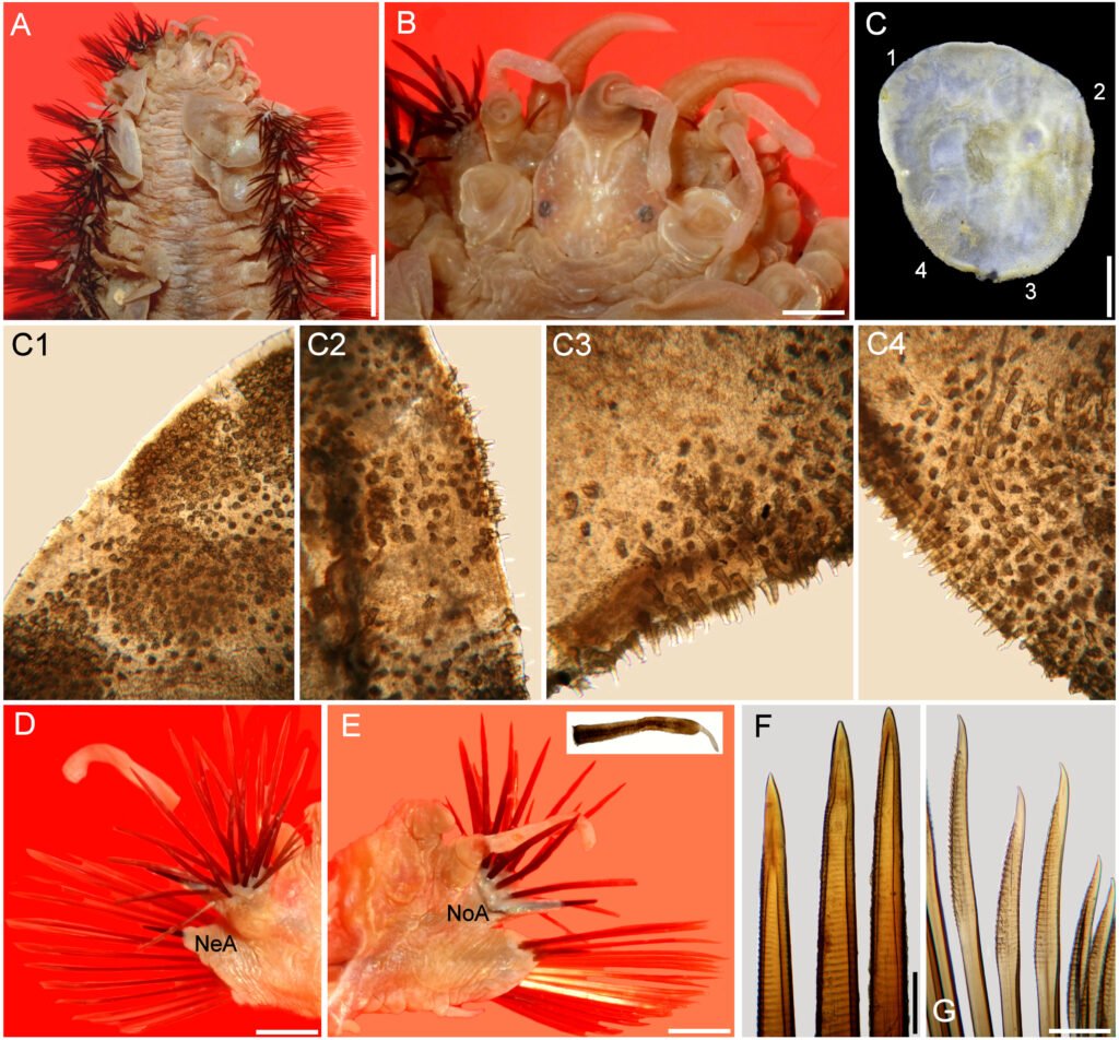
Figure 2. Hermadion magalhaensi Kinberg, 1856, topotype specimen (UMML). A, Anterior región, dorsal view; B, anterior end, dorsal view; C, right elytron 6, seen from above (1-4: sections enlarged in C1-C4); D, chaetiger 18, right parapodium, anterior view (NeA, neuracicular lobe); E, same, posterior view (inset: dorsal cirrus; NoA, notacicular lobe); F, tips of notochaetae; G, tips of neurochaetae. Scale bars: A, 2.1 mm; B, 0.6 mm; C, 1.1 mm; D, E, 1 mm; F, G, 180 µm.
Prostomium longer than wide. Eyes black, anterior eyes ventrolateral, not visible dorsally (Fig. 2B), better perceived in frontal view (Fig. 3A, B). Antennae and cirri cylindrical, tips mucronate, blunt. Median antenna with ceratophore forming a V-shaped depression, about 4 times wider than ceratostyle, ceratostyle about as long as prostomium. Lateral antennae ventral, ceratophores about half as wide as median one; ceratostyles lost. Palps thick, short, about as long as median antennae, finely papillate, but papillae not arranged in rows.
Tentacular cirri with cirrophores fused, with chaetae exposed; cirrostyles cylindrical mucronate. Facial tubercle pale, not visible dorsally, better defined after pharynx is exposed.
Elytra barely pigmented, non-fimbriate (Figs 2C, 4D), with variable amount of sediment particles. Surface covered by abundant microtubercles (Fig. 4D), small globular along anterior regions (Fig. 3C1, 2), progressively longer along posterior region, projected beyond elytral margin (Figs. 3C3, 4; 4E). Other specimens with a diffuse spot surrounding central area. Insertion area eccentric, displaced anteriorly and laterally, to the right in right elytra, to the left in left ones.

Figure 3. Hermadion magalhaensi Kinberg, 1856, topotype specimen (UMML). A, Anterior región and pharynx, dorsal view; B, anterior end, frontal view; C, pharynx opening, frontal view (Pa, papilla). Scale bars: A, 1 mm; B, 0.6 mm; C, 0.9 mm.
Parapodia biramous from segment 2. Dorsal cirri finely papillate, papillae not arranged in rows, tip smooth. Notopodia with dorsal cirri cylindrical, tip mucronate (Fig. 2D, E). Notacicular lobe projected, aciculae exposed (Fig. 4F, G). Neuropodia with neuropodial lobe projected, rarely with a long prechaetal subacicular lobe (Fig. 4G). Neuracicular lobe projected, aciculae exposed (Fig. 4F, G). Ventral cirri tapered, short, reaching base of neuracicular lobe. Nephridial lobes blunt, short, present from chaetiger 8-9, continued along body.
Notochaetae dark brown, abundant, roughly verticillate, each blunt, with series of denticles, margin finely spinulose, tips delicately bent, entire (Figs. 2F; 4H, I). Neurochaetae brownish, subdistally expanded, with rows of denticles leaving tip smooth; tip falcate, unidentate (Figs. 2G; 4J-M).
The pharynx is fully exposed; it is 9 mm long in a 46 mm long specimen (Fig. 3A). The outer surface looks maculate but the spots correspond with adsorbed crystals on the surface. The pharynx tube is slightly expanded distally, its margins are eroded and only the lateral papillae are left after erosion of most marginal integument (Fig. 3C); it was described with 9 pairs of marginal papillae. Jaws dark brown, tips blunt, without accessory denticles (Fig. 3C).
Posterior end tapered (Fig. 4C); pygidium with anus terminal; anal cirri short, resembling dorsal cirri.
Remarks
Hermadion magalhaensi Kinberg, 1856 and H. longicirratus Kinberg, 1856 were both described from the same locality and depth in Saint York Bay, Magellan Strait. The main differences between these species were that H. magalhaensi has smooth elytra, and smooth notochaetae, whereas H. longicirratus has elytra minutely tuberculate and spiny notochaetae; the former species was based on a 52 mm long specimen, whereas the latter on a 14 mm long specimen. The size difference might explain some features present in the smaller specimen and lost after abrasion in the larger specimen. However, the microtubercles in elytra might accumulate sediment and look smooth if they are not carefully cleaned. Fauvel (1916: 425) studied several specimens of different size and concluded H. magalhaensi and H. longicirratus were the same species.

Figure 4. Hermadion magalhaensi Kinberg, 1856, topotype specimen (USNM 57798). A, Whole specimen, dorsal view; B, anterior end, dorsal view; C, posterior end, dorsal view; D, right elytron from middle segment, seen from above; E, microtubercles from elytral margin; F, right cirrigerous chaetiger from middle segment, anterior view; G, right elytrigerous chaetiger from middle segment, anterior view; H, I, tips of notochaetae from middle segment; J, K, tips of supra-acicular neurochaetae from middle segment; L, M, tips of sub-acicular neurochaetae from middle segment. Scale bars: A, 3 mm; B, C, 1 mm; D, F, G, 0.5 mm; E, 0.1 mm; H-M, 50 μm.
Treadwell (1924) described Lagisca crassa from Punta Arenas, Chile based on an incomplete specimen, without most of its elytra, and included figures for the anterior end, 1 cirrigerous parapodium, and tips of 1 notochaetae (tapered), and 1 neurochaetae (unidentate), but no elytra were illustrated. Ceratostyles of antennae and dorsal cirrostyles were shown with a subdistal brown ring but were not subdistally expanded. The median antenna is longer than laterals, its base marks a deep V-shaped depression over prostomium, and the parapodium shows acicular lobes projected, but tips of aciculae were not emergent. The pharynx was indicated as having 9 pairs of marginal papillae, but no details of the jaws were provided.
On the other hand, what has been regarded as E. crassa and E. rhizoicola Hartmann-Schröder, 1962 are the 2 only species described and recorded from shallow water depths in Chile. The latter species was also described from Punta Arenas, with a 21 mm long specimen. These 2 species are very similar by having anterior eyes displaced anteriorly, similar types of noto- and neurochaetae, and dorsal cirri with black bands. They differ because in E. crassa the dorsal cirri have a single subdistal black band, against 2 in E. rhizoicola, and its tip is short, whereas it is longer in E. rhizoicola. The main difference is in the presence of fimbriae; there are no fimbriae in E. crassa, whereas E. rhizoicola has some short filaments along posterior margins. It is likely that E. rhizoicola is another junior synonym of H. magalhaensi because it resembles H. longicirratus in having longer dorsal cirri, but this might be a size dependent feature, becoming relatively shorter in larger specimens. Further, H. magalhaensi has been found living in Macrocystis rhizoids (Pratt, 1901), which was the habitat also for E. rhizoicola.
We think that the main reason for the confusion regarding the affinities between what was described as L. crassa and H. magalhaensi is because there were only 1 set of illustrations of the species (Kinberg, 1858), and since during many years, the proposals for new records or new species did not include the study of type or topotype specimens (Fauchald, 1989).
Distribution. Originally described from Puntarenas, Chile, in shallow depths (0-200 m), it ranges along subantarctic localities including the Falkland and Kerguelen Islands.
Acknowledgments
Geoff Read, Igor Jirkov and Oscar Díaz-Díaz kindly provided useful publications. William Moser found some additional field data for the Eltanin station where the specimens were found. Stéhane Hourdez and an anonymous referee carefully read this contribution and suggested several important modifications. The technical editorial issues were masterfully made by María Antonieta Arizmendi.
References
Amaral, A. C., & Nonato, E. F. (1982). Anelideos poliquetos da costa brasileira, 3. Aphroditidae e Polynoidae. Brazilia, Conselho Nacional de Desenvolvimento Científico e Tecnológico.
Annenkova, N. P. (1937). Fauna Polychaeta severnoii chasti Yaponskogo Morya. Issledovaniya Morei SSSR, 23, 139–216.
Augener, H. (1932). Antarktische und Antiboreale Polychaeten nebst einer Hirudinee. Scientific Results of the Norwegian Antarctic Expeditions 1927-1928 et sqq., instituted and financed by Consul Lars Christensen, 9, 1–85.
Averintsev, V. G. (1972). Donnye mnogotchetinkovye chervi Errantia Antarktiki i Subantarktiki no materialam sovetskoi Antarktitcheskoi Exspeditsii. Issledovaniya Fauny Morei, 11(19). Resul’taty biologicheskikh issledovanii Sovetskikh Antarktitseskikh Exspeditsii, 5, 85–293.
Baird, W. (1865). Contributions towards a monograph of the species of Annelides belonging to the Aphroditacea, containg a list of the known species, and a description of some new species contained in the National Collection of the British Museum. Journal of the Linnean Society, Zoology, 8, 172–202. https://doi.org/10.1111/j.1096-3642.1865.tb02438.x
Barnich, R., & Fiege, D. (2003). The Aphroditoidea (Annelida: Polychaeta) of the Mediterranean Sea. Abhandlungen der Senckenbergischen Naturforschenden Gesellschaft Frankfurt am Main, 559, 1–167.
Barnich, R., & Fiege, D. (2009). Revision of the genus Harmothoe Kinberg, 1856 (Polychaeta: Polynoidae) in the Northeast Atlantic. Zootaxa, 2104, 1–76. https://doi.org/10.11646/zoo
taxa.2104.1.1
Barnich, R., & Fiege, D. (2010). On the distinction of Harmothoe globifera (G.O. Sars, 1873) and some other easily confused polynoids in the NE Atlantic, with the description of a new species of Acanthicolepis Norman in McIntosh, 1900 (Polychaeta, Polynoidae). Zootaxa, 2525, 1–18. https://doi.org/10.11646/zootaxa.2525.1.1
Barnich, R., Fiege, D., Micaletto, G., & Gambi, M. C. (2006). Redescription of Harmothoe spinosa Kinberg, 1856 (Polychaeta: Polynoidae) and related species from Subantarctic and Antarctic Waters, with the erection of a new genus. Journal of Natural History, 40, 33–75. https://doi.org/10.1080/00222930500445044
Bock, G., Fiege, D., & Barnich, R. (2010). Revision of Hermadion Kinberg, 1856, with a redescription of Hermadion magalhaensi Kinberg, 1856, Adyte hialina (G.O. Sars, 1873) n. comb., and Neopolynoe acanellae (Verrill, 1881) n. comb. (Polychaeta: Polynoidae). Zootaxa, 2554, 45–61. https://doi.org/10.11646/zootaxa.2554.1.4
Dales, R. P. (1962). The polychaete stomodeum and the inter-relationships of the families of Polychaeta. Proceedings of the Zoological Society of London, 139, 389–428. https://doi.org/10.1111/j.1469-7998.1962.tb01837.x
Ehlers, E. (1897). Hamburger Magalhaensischen Sammelreise 1892/93 3(Bryozoen und Würmer). Polychaeten. Hamburg: Friederichsen & Co.
Fauchald, K. (1977). The polychaete worms: definitions and keys to the orders, families and genera. Natural History Museum of Los Angeles County, Science Series, 28, 1–188.
Fauchald, K. (1989). The second annual Riser lecture: eclecticism and the study of polychaetes. Proceedings of the Biological Society of Washington, 102, 742–752.
Fauvel, P. (1916). Annélides polychètes des Iles Falkland recueillies par M. Rupert Vallentin Esq (1902-1910). Archives de Zoologie Expérimentale et Générale, 55, 417–482. https://doi.org/10.5962/bhl.part.11511
Fauvel, P. (1923). Polychètes errantes. Faune de France, 5,1–488.
Gravier, C. (1911). Deuxième Expédition Antarctique Française (1908-1910), commandé par le Dr. Jean Charcot. Annélides polychètes. Paris: Masson et Cie.
Hartman, O. (1938). The types of the polychaete worms of the families Polynoidae and Polyodontidae in the United States National Museum and the description of a new genus. Proceedings of the United States National Museum, 86, 3046, 107–134. https://doi.org/10.5479/si.00963801.86-3046.107
Hartman, O. (1956). Polychaetous annelids erected by Treadwell, 1891 to 1948, together with a brief chronology. Bulletin of the American Museum of Natural History, 109, 239–310.
Hartman, O. (1959). Catalogue of the polychaetous annelids of the World. Allan Hancock Foundation Publications, Occasional Paper, 23, 1–628.
Hartman, O. (1964). Polychaeta Errantia of Antarctica. Antarctic Research Series, 3, 1–131. https://doi.org/10.1029/ar003
Hartmann-Schröder, G. (1962). Zur Kenntnis des Eulitorals der chilenischen Pazifikküste und der argentinischen Küste Südpatagoniens unter besonderer Berücksichtigung der Polychaeten und Ostracoden. Die Polychaeten des Eulitorals. Mitteilungen aus dem Hamburgischen Zoologischen Museum und Institut, 60, 57–270.
Imajima, M. (1997). Polychaetous annelids from Sagami Bay and Sagami Sea collected by the Emperor Showa of Japan and deposited at the Showa Memorial Institute, National Science Museum, Tokyo. Families Polynoidae and Acoetidae. National Science Museum Monographs, 13,1–131.
ICZN (International Commission of Zoological Nomenclature). (1999). International Code of Zoological Nomenclature. London, Natural History Museum. Available at: www.code.iczn.org
Jimi, N., Hookabe, N., Moritaki, T., Kimura, T., & Imura, S. (2021). First evidence of male dwarfism in scale worms: A new species of Polynoidae (Annelida) from hermit crab and molluscan shells. Journal of Zoological Systematics and Evolutionary Research, 59,801–818. https://doi.org/10.1111/jzs.12463
Jirkov, I. A. (2001). Polikhety Severnogo Ledovitogo Okeana. Tromsø, Akvaplan-Niva.
Kinberg, J. G. H. (1856). Nya slägten och arter af Annelider. Öfversigt af Kongliga Vetenskaps-Akademiens Förhhandlingar Stockholm, 12, 381–388.
Kinberg, J. G. H. (1858). Kongliga Svenska Fregatten Eugenies resa Omkring Jorden under befäl af C.A. Virgin, Ånen 1851-1853, Vetenskapliga Iakttagelser, Zoologi, 3. Annulater. Stockholm.
Levinsen, G. M. R. (1883). Systematisk-geografisk Oversigt over de nordiske Annulata, Gephyrea, Chaetognathi og Balanoglossi. Videnskabelige Meddelelser fra Dansk naturhistorisk Forening i Kjøbenhavn, 1882, 160–251. https://doi.org/10.5962/bhl.title.16117
Malmgren, A. J. (1865). Nordiska Hafs-Annulater. Öfversigt af Kongl. Vetenskaps-Akademiens Förhandlingar, 22,51–110,
M’Intosh, W. C. (1885). Report on the Annelida Polychaeta collected by H.M.S. Challenger during the years 1873-1876. Reports on the Scientific Results of the Voyage of H.M.S. Challenger during the years 1873–76, Zoology, 12,i-xxxvi.
McIntosh, W. C. (1900). A monograph of British Annelids, 1(2) Polychaeta Amphinomidae to Sigalionidae. London: Ray Society of London.
Moore, J. P. (1902). Descriptions of some new Polynoidae, with a list of other Polychaeta from North Greenland waters. Proceedings of the Academy of Natural Sciences of Philadelphia, 54, 258–278.
Moore, J. P. (1910). The polychaetous annelids dredged by the U.S.S. “Albatross” off the coast of Southern California in 1904: 2. Polynoidae, Aphroditidae and Segalionidae (sic). Proceedings of the Academy of Natural Sciences of Philadelphia, 62, 328–402.
Örsted, A. S. (1843). Grönlands Annulata dorsibranchiata. Det Kongelige Danske videnskabernes selskabs. Naturviden-
skabelige og Mathematiske Afhandlinger, 10, 153–216.
Pamungkas, J., Glasby, C. J., Read, G. B., Wilson, S. P., & Costello, M. J. (2019). Progress and perspectives in the discovery of polychaete worms (Annelida) of the world. Helgolander Marine Research, 73, 4. https://doi.org/10.1186/s10152-019-0524-z
Pettibone, M. H. (1951). A new species of polychaete worm of the family Polynoidae from Point Barrow, Alaska. Journal of the Washington Academy of Sciences, 41,44–45.
Pettibone, M. H. (1954). Marine polychaete worms from Point Barrow, Alaska, with additional records from the North Atlantic and North Pacific. Proceedings of the United States National Museum, 103, 203–356. https://doi.org/10.5479/si.00963801.103-3324.203
Pettibone, M. H. (1963). Marine polychaete worms of the New England región, 1. Families Aphroditidae through Trochochaetidae. Bulletin, United States National Museum, 227, 1–356. https://doi.org/10.5479/si.03629236.227.1
Pettibone, M. H. (1989). Two new species of Harmothoinae (Polychaeta: Polynoidae) from the East Pacific Rise, collected by Alvin dives 2000 and 2003. Proceedings of the Biological Society of Washington, 102,305–310.
Pratt, E. M. (1901). A collection of Polychaeta from the Falkland Islands. Manchester Memoirs, Memoirs and Proceeding of the Manchester Literary & Philosophical Society, 45, 1–18.
Read, G., & Fauchald, K. (Eds). (2024). World Polychaeta database. Eunoe Malmgren, 1865. Retrieved on January 17 2024, from: https://www.marinespecies.org/aphia.php?p=
taxdetails&id=129487
Rozbaczylo, N. (1985). Los anélidos poliquetos de Chile: Índice sinonímico y distribución geográfica de especies. Facultad de Ciencias Biológicas, Pontificia Universidad Católica de Chile, Monografías Biológicas, 3, 1–284.
Sars, M. (1861). Om de ved Norges Kyster forekommende Arter af Annelideslaegten Polynoë. Forhandlinger i Videnskabs-Selskabet i Christiania, 1860, 54–62.
Treadwell, A. L. (1924). A new marine annelid from Chile. Proceedings of the United States National Museum, 65, 1–3. https://doi.org/10.5479/si.00963801.65-2536.1
Uschakov, P. V. (1955). Mnogotschetinkovye chervi Dal’ne-
vostochitchykh Morei, SSSR. Akademiya Nauk, Opredeliteli ro Faune SSSR, Isdavaemye Zoologicheskim Institutom, 56, 1–445.
Uschakov, P. V. (1965). Polychaeta of the Far Eastern Seas of the U.S.S.R. Zoological Institute of the Russian Academy of Sciences, Keys to the Fauna of the U.S.S.R., 56, 1–419.
Wehe, T. (2006). Revision of the scale worms (Polychaeta: Aphroditoidea) occurring in the seas surrounding the Arabian Peninsula, 1. Polynoidae. Fauna of Arabia, 22, 23–197.
Wesenberg-Lund, E. (1962). Reports of the Lund University Chile Expedition 1948-49, 43. Polychaeta Errantia. Lunds Universitets Årsskrift, neue folge, Series 2, 57, 1–139.

Cyanoboletus abieticola (Boletaceae, Basidiomycota),a new species from Mexico
Jesús García-Jiménez a, Olivia Ayala-Vásquez a, b, Javier Isaac de la Fuente a, b,
Roberto Garibay-Orijel c, Fortunato Garza-Ocañas d, Edgardo Ulises Esquivel-Naranjo e,
Felipe Manuel Ferrusca-Rico e, Fidel Landeros e, *
a Tecnológico Nacional de México, Instituto Tecnológico de Ciudad Victoria, Boulevard Emilio Portes Gil #1301, 87010 Ciudad Victoria, Tamaulipas, Mexico
b Colegio de Postgraduados, Microbiología, Edafología, Km 36.5 Carretera México-Texcoco, Montecillo, 56230 Texcoco, Estado de México, Mexico
c Universidad Nacional Autónoma de México, Instituto de Biología, Circuito exterior s/n, Ciudad Universitaria, Coyoacán, 04510 Mexico City, Mexico
d Universidad Autónoma de Nuevo León, Campus Linares, Facultad de Ciencias Forestales, Carretera Nacional Km 145, 67700 Linares, Nuevo León, Mexico
e Universidad Autónoma de Querétaro, Facultad de Ciencias Naturales, Carretera a Chichimequillas s/n, 76140 Santiago de Querétaro, Querétaro, Mexico
*Corresponding author: landeros@uaq.mx (F. Landeros-Jaime)
Received: 1 May 2023; accepted: 25 March 2024
Abstract
Cyanoboletus abieticola is described as a new species to science. This species is characterized by the viscid pileus, cylindric to bacilliform basidiospores ([14.1] 16.2 ± 1.1 [17.5] × [5] 5.5 ± 0.3 [5.9] µm, Q [2.8] 3.0 ± 0.1 [3.2]), and its gregarious habit in mixed coniferous forests dominated by Abies religiosa or A. guatemalensis. Photographs, drawings, and the phylogenetic analysis of 3 genetic data sets (ITS, nucLSU, and RPB2) of the new species are presented.
Keywords: Boletales; Mycorrhizal fungi; “Pulveroboletus group”; Abies
© 2024 Universidad Nacional Autónoma de México, Instituto de Biología. Este es un artículo Open Access bajo la licencia CC BY-NC-ND
(http://creativecommons.org/licenses/by-nc-nd/4.0/).
Cyanoboletus abieticola (Boletaceae, Basidiomycota), una especie nueva de México
Resumen
Cyanoboletus abieticola es descrita como una especie nueva para la ciencia. Esta especie se caracteriza por el píleo víscido, basidiosporas cilíndricas a baciliformes ([14.1] 16.2 ± 1.1 [17.5] × [5] 5.5 ± 0.3 [5.9] µm, Q [2.8] 3.0 ± 0.1 [3.2]) y su hábito gregario en bosques mixtos de coníferas dominados por Abies religiosa o A. guatemalensis. Se presentan fotografías, dibujos y el análisis filogenético de 3 conjuntos de datos genéticos (ITS, nucLSU y RPB2) de la nueva especie.
Palabras clave: Boletales; Hongos ectomicorrizógenos; “Grupo Pulveroboletus”; Abies
Introduction
The family Boletaceae comprises pileate-stipitate or sequestrate species, with poroid or lamellate hymenophore. Boletaceae species are an important component of ecosystems because most of them form ectomycorrhizal associations with a great diversity of angiosperms and gymnosperms (Binder & Hibbet, 2006; Ortíz-Santana et al., 2007). They are common in different vegetation types, such as deciduous, conifer, and mixed forest; mediterranean shrublands, tropical and montane cloud forests (Bessette et al., 2010; Gelardi, 2020; Leonardi et al., 2020; Wu et al., 2016). In addition to their ecological importance, many species are valued edibles in several regions of the world (Garibay-Orijel et al., 2009; Gelardi, 2020).
Wu et al. (2014) recognized 7 major clades at the subfamily level and 59 genus-level clades, placing Boletus pulverulentus within the “Pulveroboletus group”, which also includes the genera Butyriboletus D. Arora & J.L. Frank, Cacaoporus Raspé & Vadthanarat, Caloboletus Vizzini, Crocinoboletus N.K. Zeng, Zhu L. Yang & G. Wu, Gymnogaster J.W. Cribb, Lanmaoa G. Wu & Zhu L. Yang, Pulveroboletus Murrill, Rubroboletus Kuan, Rugiboletus G. Wu & Zhu L. Yang, Suillellus Murrill, and Sutorius Halling, Nuhn & N.A. Fechner. Members of the “Pulveroboletus group” share certain common characteristics such as poroid hymenium, usually yellowish, reddish or brown hymenophore, Boletus-type hymenophoral trama (Snell & Dick, 1958), and smooth spores.
Gelardi et al. (2014) proposed the new genus Cyanoboletus, within the “Pulveroboletus group”, for those species characterized mainly by their strong blue reaction of basidiomata and context to cutting. They included 3 species in this genus: C. pulverulentus (Opat.) Gelardi, Vizzini & Simonini, C. sinopulverulentus (Gelardi & Vizzini) Gelardi, Vizzini & Simonini, and C. rainisiae (Bessette & O.K. Mill.) Gelardi, Vizzini & Simonini. The latter one was transferred to the genus Xerocomellus, but without type studies, and is currently known as X. rainisiae (Bessette & O.K. Mill.) N. Siegel, C.F. Schwarz & J.L. Frank (see discussion in Frank et al. [2020]).
Later, 4 more species were transferred to this genus: C. cyaneitinctus (Murrill) A. Farid, A.R. Franck & J.A. Bolin (Farid et al., 2021), C. instabilis (W. F. Chiu) G. Wu & Zhu L. Yang (Wu et al., 2016), C. poikilochromus (Pöder, Cetto & Zuccherelli) M. Carbone, D. Puddu & P. Alvarado (Carbone et al., 2023), and C. flavosanguineus (Lavorato & Simonini) Pierotti (Pierotti, 2015). However, the latter species was placed in the genus Neoboletus in 2021: N. flavosanguineus (Lavorato & Simonini) Biketova, Wasser, Simonini & Gelardi (Biketova et al., 2021).
Additionally, 5 Cyanoboletus species have been recently described: C. brunneoruber G. Wu & Zhu L. Yang from China (Wu et al., 2016), C. hymenoglutinosus D. Chakr., K. Das, A. Baghela, S.K. Singh & Dentinger nom. inval. from India (Li et al., 2016), C. bessettei A.R. Bessette, L.V. Kudzma, & A. Farid from the USA (Farid et al., 2021), C. macroporus Sarwar, Naseer & Khalid from Pakistan (Sarwar et al., 2021), and C. mediterraneensis Biketova, A. Rinaldi & Simonini from Israel and Italy (Biketova et al., 2016, 2022). Therefore, 10 species are currently known for the genus. These species are distributed mainly in Asia, Europe and North America and associated with Abies, Arbutus, Buxus, Carya, Castanopsis, Cistus, Crataegus, Cryptomeria, Erica, Juniperus, Lithocarpus, Ostrya, Pinus, Pistacea,and Quercus trees, as well as with Halimium shrub (Biketova et al., 2022; Farid et al., 2021; García et al., 1998; Li et al., 2016; Wu et al., 2016).
This paper describes Cyanoboletus abieticola as a new species from Mexico associated with mixed conifer forests dominated by Abies religiosa (Kunth) Schltdl. & Cham. and A. guatemalensis Rehder.
Materials and methods
Collections were carried out in central and southern Mexico (Fig. 1), in mixed coniferous forests, during the rainy season from June to October (2000-2017). Morphological characteristics were described according to Largent (1977) and Lodge et al. (2004). Chemical reactions with KOH 5% and Melzer reagent were tested on pileus, hymenophore, and stipe surface. Photographs of basidiomata were taken on site, as well as data regarding plant species. The colors for the taxonomic description were based on Kornerup and Wanscher (1978). A light microscope (Carl Zeiss GmbH 37081, Germany) was used to observe the microscopic characteristics. Only structures from mature basidiomes were measured. Twenty basidiospores, basidia, pleurocystidia, cheilocystidia and caulocystidia were measured by specimen. If the specimen consisted of several basidiomes, only the structures of 2 of them were measured. The mean of each variable of every collection was computed. Dimensions are given according to the following format: (lower mean) mean of means ± standard deviation (upper mean), Q = (lower mean) mean of means ± standard deviation (upper mean).
Vouchers were deposited in the “Herbario Nacional de México” (MEXU), in the José Castillo Tovar herbarium (ITCV), and in the mycological herbarium of the Universidad Autónoma de Querétaro (MUAQ). Additional materials were obtained in loan from the following herbaria: Escuela Nacional de Ciencias Biológicas-Instituto Politécnico Nacional herbaria (ENCB-IPN), Instituto de Biología Universidad de Guadalajara (IBUG), Instituto Nacional de Ecología (INECOL) and Universidad Autónoma de Nuevo León (UNL). All acronyms of herbaria and mycological collections follow Index Herbariorum (Thiers, 2024).
Samples of dehydrated basidiomata were used for DNA extraction. The DNA was extracted using the DNeasy Power-Soil kit (QIAGEN). Cell lysis was performed by grinding in a mortar with liquid nitrogen. Three nuclear loci (ITS, LSU and RPB2) were amplified with Platinum Taq DNA Polymerase (Invitrogen-Thermo Fisher Scientific) or Taq & Load PCR Mastermix (MP Biomedicals) in a thermal cycler (BIO-RAD). The PCR parameters were as follows: 95 ºC initial denaturation 4 min; 35 cycles of denaturation at 94 ºC for 1 min, annealing at 54 ºC for 1 min, extension at 72 ºC for 1 min, and a final extension step at 72 ºC for 10 min. The primers ITS1/ITS4 (White et al., 1990) were used for the ITS region; LR0R/LR5 (Vilgalys & Hester, 1990) for nucLSU; and RPB2-B-F2/RPB2-B-R (Wu et al., 2014) for the RPB2 gene. The PCR products were examined by 1% agarose gel electrophoresis, the gel was stained with GelRed (Biotium) and observed under an UVP Multidoc-It transilluminator (Analytikjena). Successful PCR products were cleaned with diluted 1:1 ddH2O: ExoSAP-IT (Thermo Fisher Scientific) and incubated at 37 ºC for 45 min and 80 ºC for 15 min. Sanger sequencing of clean PCR products was performed in the “Laboratorio de secuenciación genómica de la biodiversidad y la salud” at Instituto de Biología, Universidad Nacional Autónoma de México. Samples were sequenced in both directions with PCR primers using BigDye Terminator v3.1 (Thermo Fisher Scientific). Sequences were edited in Chromas Pro Vers. 1.41 (Technelysium Pty, Ltd, Tewantin, Qld, Australia).
For phylogenetic analyses we used Cyanoboletus sequences from the ITS, nucLSU and RPB2 regions listed in the Table 1. A total of 32 concatenated sequences were used (Supplementary material 1). Two Lanmaoa species were chosen as an outgroup. The sequences of each locus were aligned separately using MacClade 4.0 (Maddison & Maddison, 2000) and concatenated in Mesquite 3.40 (Maddison & Maddison, 2018). The alignments were manually edited to eliminate ambiguous regions.
Table 1
List of DNA sequences used for Cyanoboletus phylogenetic analyses.
| Species | Code | Country | GenBank | Reference | ||
| ITS | nucLSU | RPB2 | ||||
| Lanmaoa sublurida | USF 288426 | USA | MW675740 | MW662575 | MW737499 | Farid et al., 2021 |
| L. sublurida | USF 300104 | USA | MW675736 | MW662572 | MW737498 | Farid et al., 2021 |
| Cyanoboletus abieticola | MUAQ13 Paratype | Mexico | MW750332 | MW750369 | – | This study |
| C. abieticola | ITCV-1010 Paratype | Mexico | – | MW750367 | – | This study |
| C. abieticola | MEXU-30111 Paratype | Mexico | MW209739 | MW750366 | PP108649 | This study |
| C. abieticola | MEXU-30106 Paratype | Mexico | MW209740 | MW750365 | – | This study |
| C. abieticola | MEXU-30109 Holotype | Mexico | MW209738 | MW750368 | PP108650 | This study |
| Table 1. Continued | ||||||
| Species | Code | Country | GenBank | Reference | ||
| ITS | nucLSU | RPB2 | ||||
| C. abieticola | MEXU-26275 Paratype | Mexico | KC152077 | – | – | This study |
| C. abieticola | MEXU-26276 Paratype | Mexico | KC152076 | – | – | This study |
| C. abieticola | MEXU-26278 Paratype | Mexico | KC152075 | – | – | This study |
| C. bessettei | USF 301500 (A) Holotype | USA | MW675737 | MW662571 | MW737457 | Farid et al., 2021 |
| C. bessettei | USF 301500 (B) Holotype | USA | MW675738 | – | MW737458 | Farid et al., 2021 |
| C. brunneoruber | HKAS63504 | China | – | KF112368 | KF112702 | Wu et al., 2014 |
| C. brunneoruber | HKAS80579 1 | China | – | KT990568 | KT990401 | Wu et al., 2016 |
| C. brunneoruber | HKAS80579 2 | China | – | KT990569 | KT990402 | Wu et al., 2016 |
| C. cyaneitinctus | USF 288424 | USA | MW675739 | MW662574 | MW737461 | Farid et al., 2021 |
| C. cyaneitinctus | USF 301499 Epitype | USA | MW675744 | MW662579 | MW737503 | Farid et al., 2021 |
| C. cyaneitinctus | JAB184 | USA | MW675731 | MW662584 | MW737467 | Farid et al., 2021 |
| C. cyaneitinctus | JAB324 | USA | MW675732 | MW662586 | MW737469 | Farid et al., 2021 |
| C. cyaneitinctus | JAB325 | USA | MW675733 | – | MW737470 | Farid et al., 2021 |
| C. hymenoglutinosus | AB2016 | India | KT907355 | KT860060 | – | Li et al., 2016 |
| C. instabilis | FHMU1839 | China | MG030473 | MG030466 | – | Chai et al., 2018 |
| C. instabilis | HKAS59554 | China | – | KF112412 | KF112698 | Wu et al., 2014 |
| C. macroporus | DC21-02 | India | OQ860238 | OQ860239 | ON364552 | Das et al., 2023 |
| C. macroporus | DC21-04 | India | OQ860240 | OQ860241 | OQ876894 | Das et al., 2023 |
| C. mediterraneensis | K-M000265123 Holotype | Israel | – | OM801212 | – | Biketova et al., 2023 |
| C. mediterraneensis | K-M000265124 Paratype | Israel | OM801199 | – | – | Biketova et al., 2023 |
| C. mediterraneensis | TUR-A 209199 | Italy | MZ265183 | MZ265198 | MZ277228 | Carbone et al., unpublished |
| C. paurianus | KD22-008 | India | – | OQ859920 | OQ914389 | Das et al., 2023 |
| C. paurianus | KD22-009 Holotype | India | – | OQ859919 | OQ914388 | Das et al., 2023 |
| C. poikilochromus | GS10070 | Italy | KT157051 | KT157060 | KT157068 | Gelardi et al., 2015 |
| C. poikilochromus | GS11008 | Italy | KT157050 | KT157059 | KT157067 | Gelardi et al., 2015 |
| C. poikilochromus | TO HG 100091987 Epitype | Italy | KT157047 | KT157056 | – | Gelardi et al., 2015 |
| C. pulverulentus | MG126a | Italy | KT157053 | KT157062 | – | Gelardi et al., 2015 |
| C. pulverulentus | MG 456a | Portugal | KT157054 | KT157063 | – | Gelardi et al., 2015 |
| C. pulverulentus | MG 628a | Italy | KT157055 | KT157064 | KY157069 | Gelardi et al., 2015 |
| C. sinopulverulentus | HKAS59609 | China | – | KF112366 | KF112700 | Wu et al., 2014 |
| C. sinopulverulentus | HMAS266894 | China | KC579402 | – | – | Gelardi et al., 2015 |
| Cyanoboletus. sp. | HKAS76850 | China | – | KF112343 | KF112697 | Wu et al., 2014 |
Phylogenetic analyses were partitioned for both Maximum Likelihood (ML) and Bayesian Inference (BI) analyses. Best evolutionary models were selected with jModelTest 2.1.10 (Darriba et al., 2012), using the Akaike information criteria. Table 2 summarizes the evolutionary model of each region. The ML analysis was performed in RAxML 7.2.6 (Stamatakis, 2006), with 1,000 bootstrap replicates. The BI analysis was performed in MrBayes 3.2.5 (Ronquist & Huelsenbeck, 2003) with 5,000,000 generations, 4 Monte Carlo chains and sampling every 100 trees, chain convergence was determined using Tracer 1.7.2 (Rambaut et al., 2018), we discarded the first 25% of trees as burning. ML bootstrap support (BS) over 50% and Bayesian posterior probability (PP) values exceeding 0.90 are reported in the resulting tree.
Table 2
Nucleotide substitutions models by each partition obtained from jModelTest with the corrected Akaike information criterion.
| Gene/Partition | Length | Evolutifon model | Nst-rates |
| nucLSU | 747 pb | TIM1+G | 6 – Gamma |
| ITS | 603 pb | TPM3ef+G | 6 – Gamma |
| RPB2 | 688 pb | TIM3ef+G | 6 – Gamma |
Results
The phylogenetic analyses (Fig. 1) based on the ITS, nucLSU and RPB2 concatenated dataset using ML analyses and BI showed that all Cyanoboletus species cluster in a monophyletic clade with strong support (PP 1 / BS 100). Trees obtained from separate ITS and RPB2 analyses are presented in Supplementary material 2. Sequences of all C. abieticola sp. nov. samples form a strongly supported clade (PP 1/BS 99) within the genus Cyanoboletus. Consequently, based on morphological, phylogenetic and ecological data, we describe it as a new species, which is also the first species of the genus Cyanoboletus reported from Mexico.
To determine whether the ITS or RPB2 region is more informative as a barcode, in Table 3 we show the percentages of nucleotide similarity between species. The RPB2 region commonly has more variation and generates fewer ambiguous regions than the ITS. Even while the ITS region has been considered as the fungal genetic barcode, the RPB2 region has higher resolution for species delineation in Cyanoboletus.
Description
Cyanoboletus abieticola J. García, Ayala-Vásquez & Landeros,sp. nov.
Diagnosis. Pileus 13-50 mm in diameter, viscid, widely convex, convex to plane convex, brown, yellow, pale brown, reddish-brown, cinnamon. Stipe 40-75 × 7-8 mm, viscid, cylindrical, yellow when young, middle section and apex yellow when mature, basal area red brown to red-vinaceous, and basidiospores (14.1) 16.2 ± 1.1 (17.5) × (5) 5.5 ± 0.3 (5.9) µm. It grows on the ground of neotropical Abies forests.
Description. Macroscopic characters (Fig. 2). Pileus 13-50 mm diameter, widely convex, convex to plane convex, brown yellow (4B6), pale brown (6B5), reddish-brown, cinnamon, furfuraceous, very viscid when young, incurved margin, sterile. Hymenophore attached, pores 0.3-0.7 mm in diameter, pale yellow (2A8-2A4), yellow (3A8) to yellow-olive (30B8-30B7) it stains dark blue (22F8) when touched, with some brown tones, young specimens exude a somewhat acidic astringent-flavored yellow liquid from hymenophore; tubes 2-6 mm diameter, concolor to pores, immediately changing to dark blue (25F8) when cut. Context white, 5 mm thick, dark blue (22F8) when cut; stipe context pale yellow (3A6) base red-vinaceous (10F8), turning blue (25F8) when cut. Stipe 40-75 × 7-8 mm, cylindrical, yellow when young, middle section and apex yellow when mature, basal area red brown (9C8-9C5) to red-vinaceous (10F8), surface pruinose to furfuraceous, immediately turning dark blue (22F8) when touched. Mycelium white.
Chemical reactions: pileus surface and context turning dark brown (6F8) with KOH 5%, hymenophore turning brown (5F3) with KOH 5%.
Microscopic characters (Fig. 3). Basidiospores 14.1-17.5 × 5-5.9 µm, mean values 16.2 ± 1.1 × 5.5 ± 0.3 µm, Q 2.8-3.2, means values 3.0 ± 0.1, cylindric to bacilliform, yellow in KOH, inamyloid with Melzer’s reagent, with visible suprahilar depression (Fig. 3A). Basidia 27.3-37.6 × 9.5-10.7 µm, mean values 33.3 ± 4.0 × 10.3 ± 0.5 µm, clavate, hyaline in KOH, tetrasporic (Fig. 3B). Hymenophoral trama divergent (Boletus-type), with a medium and lateral stratum of cylindrical hyphae, hyaline to yellowish brown in KOH, inamyloid with Melzer’s reagent, with gelatinized wall. Pleurocystidia 52.2-71.2 × 10.6-13.9 µm, mean values 63.2 ± 7.5 × 12.4 ± 1.4 µm, arise from subhymenium, mucronate, clavate, fusoid-ventricose, hyaline to brown in KOH (Fig. 3C), with reddish brown incrustations on Melzer. Cheilocystidia 39.6-58.4 × 8.9-11 µm, mean values 47.7 ± 7.5 × 9.9 ± 0.8 µm, fusoid-ventricose, mucronate, clavate, reddish to brown on KOH, with reddish brown incrustations (dextrinoid) in Melzer’s reagent, thick-walled (Fig. 3D). Pileipellis formed by an ixotrichoderm 250-300 µm thick, with terminal cells 34.8-45.4 × 4-5.6 µm, mean values 38.4 ± 4.8 × 4.7 ± 0.6 µm, cylindrical, yellow-reddish brown in KOH, reddish brown (dextrinoid) with Melzer’s reagent, some with thick wall, sometimes gelatinized (Fig. 3E). Stipitipellis 100-120 µm thick, ixocutis, hyphae subparallel to loosely intermingled, formed of caulocystidia 34-47 × 9.6-11.4 µm, mean values 40.6 ± 5.2 × 10.3 ± 0.7 µm, in clusters, fusoid-mucronate, clavate, some ventricose, arise from the middle or surface, hyaline to brown in KOH, with reddish brown incrustations (dextrinoid) in Melzer’s reagent.

Figure 1. Bayesian tree using the concatenated alignment (LSU, ITS and RPB2). The values in the phylogram branches represent the maximum likelihood bootstrap (MLB)/Bayesian posterior probabilities (BPP). Only MLB 50 ≥ and 90 BPP ≥ are displayed. Cyanoboletus abieticola is in bold.
Taxonomic summary
Holotype: Mexico, Oaxaca, Santa Catarina Ixtepeji, La Cumbre, Abies guatemalensis, 17º11’ N, 96º38’ W, 2,902 m asl, 4 November 2017, Ayala-Vásquez (MEXU-30109).
Isotype: ITCV-1141
Mycobank: MB 838523.
Etymology: the name of the species is due to its association with Abies forests.
Habitat: scattered or solitary in mixed neotropical conifer forests dominated by Abies religiosa and A. guatemalensis.
Table 3
Percent nucleotide similarity between Cyanoboletus species based on their sequences, ITS/RPB2 DNA sequences. Above ITS and below RPB2 percentage ranges (WD: without data).
| C. abieticola | C. bessettei | C. brunneoruber | C. cyaneitinctus | C. hymenoglutinosusus | C. instabilis | C. macroporus | C. mediterraneensis | C. paurianus | C. poikilochromus | C. pulverulentus | C. sinopulverulentus | |
| C. abieticola | 0.0-0.5 0.0 | |||||||||||
| C. bessettei | 5.6-6.2 8.7 | 0.0 0.0 | ||||||||||
| C. brunneoruber | WD 5.9 | WD 8.7 | WD 0.0 | |||||||||
| C. cyaneitinctus | 6.7-7.2 7.0 | 8.1 10.2 | WD 5.9 | 0.0 0.0 | ||||||||
| C. hymenoglutinosus | 3.6-3.9 WD | 4.6 WD | WD WD | 5.7 WD | WD WD | |||||||
| C. instabilis | 5.7-7.0 7.5 | 5.7 8.3 | WD 7.8 | 6.3 8.7 | 6.3 WD | WD WD | ||||||
| C. macroporus | 4.4-4.6 6.0 | 5.4 8.8 | WD 5.3 | 4.9 3.6 | 1.8 WD | 7.0 7.9 | 0.0 0.0 | |||||
| C. mediterraneensis | 2.9-3.9 2.7 | 2.9-3.4 7.0 | WD 5.4 | 2.0-5.9 6.0 | 2.3 WD | 5.1 5.8 | 3.1-3.2 5.4 | 0.0-0.3 WD | ||||
| C. paurianus | WD 6.2 | WD 9.2 | WD 4.6 | WD 3.6 | WD WD | WD 8.0 | WD 2.7 | WD 4.9 | WD 0.0 | |||
| C. poikilochromus | 4.2-5.9 6.9-7.1 | 3.9 8.5-8.7 | WD 7.1-7.4 | 5.9-7.6 7.7-7.8 | 2.0-3.4 WD | 7.0-7.1 7.8-8.0 | 3.3-4.6 7.5 | 1.7-3.0 6.3-6.7 | WD 7.1-7.2 | 0.0 0.0-0.5 | ||
| C. pulverulentus | 3.6-3.9 6.5 | 4.9-5.2 9.1 | WD 5.2 | 4.6 2.2 | 2.1-2.3 WD | 6.3 8.4 | 1.8-2.1 2.8 | 2.3-2.8 5.1 | WD 2.8 | 3.6-4.9 7.8 | 0.0-0.3 WD | |
| C. sinopulverulentus | 3.8-4.1 6.1 | 5.2 9.3 | WD 4.6 | 4.0 3.9 | 2.8 WD | 6.3 7.4 | 1.0 2.7 | 2.3-3.1 4.7 | WD 2.1 | 3.1-4.7 7.0-7.1 | 1.3-1.6 3.3 | WD WD |
Additional material studied. Mexico, Hidalgo: El Chico National Park, Abies religiosa, 13 August 1988, J. García (ITCV-5874), 13 August 1988, J. García (ITCV-5878), 23 August 2018, J. García (ITCV-21996); Jalisco: Road to Tamazula, 15 km to Mazamitla, between Guayabos and Cabañas, A. religiosa, 24 August 1974, G. Guzmán (ENCB-11869); Road from San Sebastián del Oeste to Santa Ana, A. religiosa, 29 August 1994, L. Guzmán-Dávalos (IBUG-5349); Nevado de Colima, A. religiosa, 13 October 1984, A. Tamayo and R. González (IBUG); 11 August 1990, J. García (ITCV-6633); Estado de México: Road to Chalma, Lagunas de Zempoala National Park, A. religiosa, 1 August 1982, R. E. Chio (ENCB-368, ITCV-368), 23 September 1985, E. Perez-Silva (MEXU-19733), 17 July 1985, García (ITCV-4784); Nevado de Toluca National Park, near Ranchería La Puerta, A. religiosa, 21 August 1983, L. Colón 208-a (ENCB); Naucalpan-Toluca highway, road to Villa Alpina, La Glorieta, A. religiosa, without date, A. González-Velázquez (ENCB-965); Mpio. Amanalco, Corral de Piedras, A. religiosa, without date, A. González-Velázquez (ENCB-1454); Zone E of San Rafael Atlixco, Escualango, A. religiosa, 7 October 1983, A. Hernández (ENCB-145); La Marquesa, A. religiosa, 7 July 1963, Gispert-Imaz (MEXU-9873), 12 August 1962, G. Guzman (ENCB-3198); Ciudad de México: Former Mexico-Cuernavaca highway 3 km S. of Parres, A. religiosa, 17 July 1982, S. Chacón (ENCB-183); Michoacán: Morelia-Cd Road. Hidalgo, Sierra de Mil Cumbres, km 45, A. religiosa, 21 July 1983, J. García (UNL-3665, ITCV-3665), 15 July 1982, J. García (UNL-1998, ITCV-1998); Morelos: Road to Chalma, 5 km Huitzilac, A. religiosa, 17 July 1982, S. Chacón (ENCB-234); Oaxaca: Santa Catarina Ixtepeji, La Cumbre, 17°11’ N, 96°38’ W, A. guatemalensis, 18 July 2017, Ayala-Vásquez (ITCV-846), 20 August 2017, Ayala-Vásquez (ITCV-1002), 21 August 2017, Ayala-Vásquez and Victores-Aguirre, (ITCV-1010); 8 October 2017, Ayala-Vásquez, (MEXU-30106, ITCV-1129), Ayala-Vásquez (MEXU-30111, ITCV-1128); 4 November 2017, Ayala-Vásquez (ITCV-1136); Ayala-Vásquez (MEXU-30109, ITCV-1141), Ayala-Vásquez, (ITCV-1142); Querétaro: Mpio. Cerro El Zamorano, A. religiosa, 16 September 1995, J. García (ITCV-9560), 23 September 2017, Ferrusca 390 (MUAQ13), 19 october 2019, Ferrusca 462 (MUAQ14), Ferrusca 467 (MUAQ15), 16 september 2022, Landeros 3770 (MUAQ16); Tlaxcala: road from Tlaxco to Chignahuapan, Cerro de Teapa, El Conejo, A. religiosa, 26 June 1979, J. García (UNL-496, ITCV-496); Huamantla, road to La Malinche hilltop, A. religiosa, 29 August 2010, T. Bruns (MEXU-26275) (MEXU-26276) (MEXU-26278); Veracruz: Xico, Los Gallos, 1.5 km to N. from Ingenio El Rosario, Zona del Cofre de Perote, A. religiosa, 27 October 1983, Villarreal 1024 (INECOL-1068), 31 July 1990, J. García (ITCV-6459).
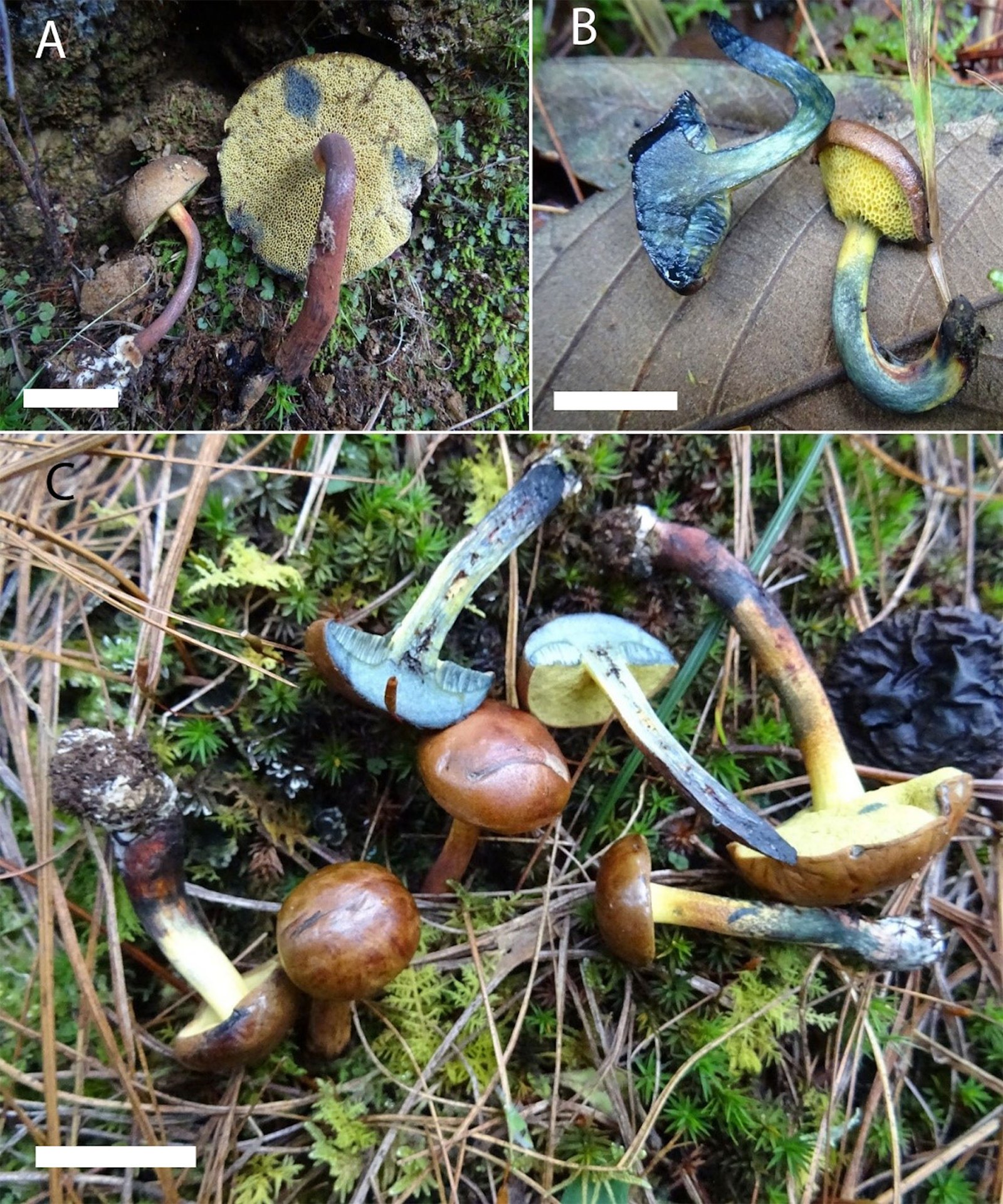
Figure 2. Cyanoboletus abieticola morphology. A) Basidiomata (holotype), B) context, C) basidiomata at different stages. Bar = 10 mm.

Figure 3. Microscopic characteristics of Cyanoboletus abieticola. A) Basidiospores, B) basidia, C) cheilocystidia, D) pleurocystidia, E) stipitipellis, F) pileipellis. Bar = 10 µm.
Remarks
Cyanoboletus abieticola is a new species with a strong phylogenetic support (PP1 / BS 99) and distinctive taxonomic characters. This species is characterized by a small pileus 13-50 mm diameter, very viscid, pale brown, yellowish-brown, brown, red to cinnamon; pileus sterile margin somewhat involute when young; hymenophore distills a liquid with sweaty acidic flavor when young, pores and tubes yellow; stipe yellow cylindrical in the middle and apex, basal area red brown to red-vinaceous, when touched immediately turns to dark blue. It is distributed in mixed coniferous forests in central and southern Mexico at altitudes ranging from 2,700 to 3,000 m asl (Fig. 4).

Figure 4. Distribution of Cyanoboletus abieticola in Mexico.
Previously, only 2 species of Cyanoboletus (C. bessettei and C. cyaneitinctus) have been recorded from North America (Farid et al., 2021). Cyanoboletus bessettei and C. cyaneitinctus have similar small basidiomata as C. abieticola, nevertheless, both species are associated with oak forests in the United States, in contrast, C. abieticola is distributed from central to southern Mexico in mixed conifer forests with a strong association with Abies. Morphological and microscopical comparisons of the American species of Cyanoboletus are shown in the Table 4. They are similar by morphology, however, C. bessettei has blue-green then reddish-brown staining in its stipe when handled, while C. abieticola and C. cyaneitinctus are bluing, also their basidiospores are bigger than those in C. bessettei (9-11 ´ 3.5-5 mm). Cyanoboletus cyaneitinctus and C. abieticola are very similar by morphology and microscopical characters, however they are not phylogenetically close, and the first one has shorter basidiospores in length (11.5-15 mm) and associates with Carya and Quercus.
Table 4
North American Cyanoboletus species morphology comparison.
| Characteristic | C. bessettei | C. cyaneitinctus | C. abieticola |
| Pileus color | Buffy brown when young, darker brownish at maturity | Bister, umber, mahogany and dark brown | Brown yellow, pale brown, reddish brown, cinnamon |
| Pileus size | 2.7-8 cm wide | 3-8 cm wide | 1.3-5 cm wide |
| Staining stipe when handled | Blue-green then reddish-brown | Bluing instantly and strongly | Bluing instantly and strongly |
| Stipe size | 2.5-4 × 1-2 cm | 3-6 × 0.5-2 cm | 4-7.5 × 0.7-0.8 cm |
| Basidia | (2)4-spored | 4-spored | 4-spored |
| Basidiospores | (8-)9-11(-12) × 3.5-5 mm | (11)11.5-15(16) × 4-6 mm | [(14.1) 16.2 ± 1.1 (17.5) × (5) 5.5 ± 0.3 (5.9) µm |
| Host plants | Under Quercus and Pinus | Under Carya and Quercus | Under Abies spp. |
Most Cyanoboletus species are morphologically similar, so to separate them, a combination of microscopic, geographic and molecular characteristics is necessary. With the description of this new species, the genus Cyanoboletus reaches its southernmost distribution in America, developing in forests of central and southern Mexico forests. Its occurrence in Abies forests is also highlighted, since in North America the genus has been recorded in mixed Pinus–Quercus forests (Farid et al., 2021).
Acknowledgements
We thank Instituto Tecnológico de Ciudad Victoria, Universidad de Quintana Roo, Universidad Nacional Autónoma de México and Universidad Autónoma de Nuevo León for supporting this research. The DNA sequences produced at IB-UNAM were financed by project Conacyt 239266 assigned to RGO. AVO thanks Conahcyt for the postdoctoral funding 3129307. The last author wants to thank the Universidad Autónoma de Querétaro for the project FNB-2022-06.
References
Bessette, A., Roody, W. C., & Bessette, A. R. (2010). Boletes of Eastern North America: a color guide to the fleshy pored mushrooms. China: Syracuse University Press.
Biketova, A. Y., Kosakyan, A., Wasser S. P., & Nevo, E. (2016). New, noteworthy, and rare species of the genus Boletus in Israel. Plant Biosystems, 150, 876–886. https://doi.org/10.1080/11263504.2014.990537
Biketova, A. Y., Wasser, S. P., Simonini, G., & Gelardi, M. (2021). Nomenclatural novelties: Neoboletus flavosanguineus (Lavorato & Simonini) Biketova, Wasser, Simonini & Gelardi, comb.nov. Index Fungorum, 505, 1.
Biketova A. Y., Rinaldi A. C., & Simonini, G. (2022). Nomenclatural novelties: Cyanoboletus mediterraneensis Biketova, A. Rinaldi & Simonini, sp. nov. Index Fungorum, 516, 1.
Binder, M., & Hibbett, D. S. (2006). Molecular systematics and biological diversification of Boletales. Mycologia, 98, 971–983. https://doi.org/10.1080/15572536.2006.11832
626
Carbone, M., Puddu, D., & Alvarado, P. (2023). Nomenclatural novelties: Cyanoboletus poikilochromus (Pöder, Cetto & Zuccherelli) M. Carbone, D. Puddu & P. Alvarado, comb. nov. Index Fungorum, 534, 1.
Darriba, D., Taboada, G. L., Doallo, R., & Posada, R. (2012). jModelTest 2: more models, new heuristics and parallel computing. Nature Methods, 9, 772.
Farid, A., Bessette, A. E., Bessette, A. R., Bolin, J. A., Kudzma, L. V. Franck, A. R. et al. (2021). Investigations in the boletes (Boletaceae) of southeastern USA: four novel species and three novel combinations. Mycosphere, 12, 1038–1076. https://doi.org/10.5943/mycosphere/12/1/12
Frank, J. L., Siegel, N., Schwarz, C. F., Araki, B., & Vellinga, E. C. (2020). Xerocomellus (Boletaceae) in western North America. Fungal Systematics and Evolution, 5, 265–288. http://dx.doi.org/10.3114/fuse.2020.06.13
García, J., Pedraza, D., Silva, C. I., Andrade, R. L., & Castillo, J. (1998). Hongos del estado de Querétaro. Querétaro: Universidad Autónoma de Querétaro.
Garibay-Orijel, R., Martínez-Ramos, M., & Cifuentes, J. (2009). Disponibilidad de esporomas de hongos comestibles en los bosques de pino encino de Ixtlán de Juárez, Oaxaca. Revista Mexicana de Biodiversidad, 80, 521–534. https://doi.org/10.22201/ib.20078706e.2009.002.615
Gelardi, M. (2020). Diversity, biogeographic distribution, ecology, and ectomycorrhizal relationships of the edible porcini mushrooms (Boletus s. str., Boletaceae) worldwide: state of the art and an annotated checklist. In J. Pérez-Moreno, A. Guerin-Laguette, R. Flores Arzú, & F.Q. Yu (Eds.), Mushrooms, humans and nature in a changing World (pp. 223–271). Cham, Switzerland: Springer. https://doi.org/10.1007/978-3-030-37378-8_8
Kornerup, A., & Wanscher, J. H. (1978). Methuen handbook of colour. London: Methuen Publishing.
Largent, D., Johnson, D., & Watling, R. (1977). How identify mushrooms to genus III: microscopic features. Eureka, California: Mad River Press.
Leonardi, M., Marinho-Furtado, A. N., Comandini, O., Geml, J., & Rinaldi, A. C. (2020). Halimium as an ectomycorrhizal symbiont: new records and an appreciation of known fungal diversity. Mycological Progress, 19, 1495–1509. https://doi.org/10.1007/s11557-020-01641-0
Li, G. J., Hyde, K. D., Zhao, R. L., Hongsanan, S., Abdel-Aziz, F. A., Abdel-Wahab, M. A. et al. (2016). Fungal diversity notes 253-366: taxonomic and phylogenetic contributions to fungal taxa. Fungal Diversity, 78, 1–237. http://doi.org/10.1007/s13225-016-0366-9
Lodge, D. J., Ammirati, J. F., Dell, T. O., & Mueller, G. M. (2004). Terrestrial and lignicolous macrofungi: collecting and describing macrofungi. In G. Mueller, G. F. Bills, & M. S. Foster (Eds.), Biodiversity of Fungi. Inventary and monitoring methods (pp. 128–158). New York: Elsevier Academic Press.
Maddison, D. R., & Maddison, W. P. (2000). MacClade 4: analysis of phylogeny and character evolution. Sunderland, Massachussetts: Sinauer Associates.
Maddison, W. P., & Maddison, D. R. (2018). Mesquite: a modular system for evolutionary analysis. Version 3.40. http://www.mesquiteproject.org
Pierotti, A. (2015). Nomenclatural novelties: Cyanoboletus flavosanguineus (Lavorato & Simonini), in Pierotti, comb. nov. Index Fungorum, 263, 1.
Rambaut, A., Drummond, A. J., Xie, D., Baele, G., & Suchard, M. A. (2018). Posterior summarization in Bayesian phylogenetics using Tracer 1.7. Systematic Biology, 67, 901-904. http://doi.org/10.1093/sysbio/syy032
Ronquist, F., & Huelsenbeck, J. P. (2003). MrBayes 3: Bayesian phylogenetic inference under mixed models. Bioinformatics, 19, 1572–1574. https://doi.org/10.1093/bioinformatics/btg180
Sawar, S., Naaser, N., & Khalid, A. N. (2021). Cyanoboletus macroporus (Boletaceae), a new bolete species from Pakistani forests. Karstenia, 59, 78–87.
Snell, W. H., & Dick, E. A. (1958). Notes on Boletes X. A few miscellaneous discussions and a new species. Mycologia, 50, 57–65. https://doi.org/10.1080/00275514.1958.12024709
Stamatakis, A. (2006). RAxML-VI-HPC: maximum likelihood-based phylogenetic analyses with thousands of taxa and mixed models. Bioinformatics, 22, 2688–2690. https://doi.org/10.1093/bioinformatics/btl446
Thiers, B. M. (2024). Index Herbariorum. Retrieved on March 03rd, 2024 from: https://sweetgum.nybg.org/science/ih/
Vizzini, A. (2014). Nomenclatural novelties: Cyanoboletus Gelardi, Vizzini & Simonini, gen. nov. Index Fungorum, 176, 1.
Wu, G., Feng, B., Xu, J. P., Zhu, X. T., Li, Y. C., Zeng, N. K., Hosen, M. I., & Yang, Z. L. (2014). Molecular phylogenetic analyses redefine seven major clades and reveal 22 new generic clades in the fungal family Boletaceae. Fungal Diversity, 69, 93–115. https://doi.org/10.1007/s13225-014-0283-8
Wu, G., Li, Y. C., Zhu, X. T., Zhao, K., Han, L. H, Cui, Y. Y., Li, F., Xu, J. P., & Yang, Z. L. (2016). One hundred noteworthy boletes from China. Fungal Diversity, 81, 25–188. https://doi.org/10.1007/s13225-016-0375-8

A new species of Lysinoe (Gastropoda: Helicoidea) from the Oligocene of Mexico
Rodrigo B. Salvador *
UiT – The Arctic University of Norway, The Arctic University Museum of Norway, Lars Thørings veg 10, 9006 Tromsø, Norway
University of Helsinki, Finnish Museum of Natural Zoology Unit, Pohjoinen Rautatiekatu 13, 00100 Helsinki, Finland
*Corresponding author: salvador.rodrigo.b@gmail.com (R.B. Salvador)
Received: 27 November 2023; accepted: 23 May 2024
http://zoobank.org/urn:lsid:zoobank.org:pub:6F009397-AD47-4995-8790-223A97819748
Abstract
In her 1945 study on the Tertiary fossil mollusks of northeastern Mexico, Gardner listed only 2 taxa of land snails: Holospira eva Gardner, 1945 and “Helix” sp. The latter is recognized here as a new species of Lysinoe Adams & Adams, 1855 (Helicoidea, Xanthonychidae). The new species can be diagnosed from its congeners by its flattened shell profile, a lower body whorl with a faint angulation on its median portion, a ridge-like angulation around the umbilicus, and a likely wide umbilicus. The species is known to occur in 2 nearby Upper Middle Oligocene outcrops in the eastern part of the state of Nuevo León.
Keywords: Mollusca; Land snail; Fossil; Nuevo León; Stylommatophora; Xanthonychidae
© 2024 Universidad Nacional Autónoma de México, Instituto de Biología. Este es un artículo Open Access bajo la licencia CC BY-NC-ND
(http://creativecommons.org/licenses/by-nc-nd/4.0/).
Una especie nueva de Lysinoe (Gastropoda: Helicoidea) del Oligoceno de México
Resumen
En su estudio de 1945 sobre los moluscos fósiles del Terciario del noreste de México, Gardner enumeró solo 2 taxones de caracoles terrestres: Holospira eva Gardner, 1945 y “Helix” sp. Esta última se reconoce aquí como una especie nueva de Lysinoe Adams et Adams, 1855 (Helicoidea, Xanthonychidae). La nueva especie se puede diagnosticar a partir de sus congéneres por el perfil aplanado de su concha, la vuelta del cuerpo es más baja y con una leve angulación en su porción media, una angulación en forma de cresta alrededor del ombligo y un ombligo probablemente ancho. La especie se encuentra en 2 afloramientos cercanos del Oligoceno Medio Superior en la parte oriental del estado de Nuevo León.
Palabras clave: Mollusca; Caracol terrestre; Fósil; Nuevo León; Stylommatophora; Xanthonychidae
Introduction
In 1945, Julia Gardner published an important paper describing the Tertiary fossil molluscan fauna of northeastern Mexico (Gardner, 1945), with information and specimens collected by the United States Geological Survey (USGS). Virtually all fossils were marine or freshwater, with 2 exceptions: the land snail taxa Holospira eva Gardner, 1945 (Urocoptidae) and “Helix” sp.
Gardner (1945) assigned the fossils the broad identity of “Helix” sp. to signify they were helicoid snails (superfamily Helicoidea). Still, she alluded to the possibility that those fossils were closely related to the Mexican and Central American genus Lysinoe Adams & Adams, 1855 (Helicoidea, Helminthoglyptidae). Later, Roth (1984) described a new species, Lysinoe breedlovei Roth, 1984, from the Vieja Group (Upper Eocene; Texas, USA) and included Gardner’s “Helix” sp. in that species. It is uncertain why Roth (1984) did that, as the morphological differences between his new species and Gardner’s “Helix” sp. are quite striking. Furthermore, the discrepancy in age between the 2, alongside the large geographical distance, would also have been good indicators that they were 2 separate species.
Herein, Gardner’s “Helix” sp. is recognized as a distinct species belonging to the genus Lysinoe and described as new.
Materials and methods
The single specimen representative of the new species is housed in the Paleobiology Collection of the National Museum of Natural History (NMNH, Smithsonian Institution, Washington D.C., USA) under the registration number USNM MO 497132. A historical background and further details regarding the USGS collection efforts in Mexico can be found in Gardner (1945).
Description
Family Xanthonychidae Strebel & Pfeffer, 1880
Genus Lysinoe Adams & Adams, 1855 (type species Helix ghiesbreghti Nyst, 1841)
Lysinoe bravoensis sp. nov. (Fig. 1)
http://zoobank.org/urn:lsid:zoobank.org:act:2DC2392E-CBCF-4C66-AED4-CC8924D9CC2D
Shell large (height 23.0 mm, width 41.3 mm), helicoid, of ca. 4 whorls, with a low spire. Whorls growing regularly in size, but final ½ whorl suddenly expands towards aperture. Body whorl slightly flattened, with faint angulation on its median portion and light ridge-like angulation around the umbilicus. Aperture seemingly rounded, prosocline. Umbilicus seemingly deep and relatively wide. The fossil is an internal mold, so not all shell structures can be observed; features such as the umbilicus’ width might be misleading.
Even though Gardner (1945: 18, 267) alludes to further material, no specimens beyond the holotype (Gardner’s figured specimens) were available for study at the NMNH. According to that author’s remarks, a few additional morphological features could be gleaned from the specimens then available (Gardner, 1945: 267): the number of whorls could grow a little beyond 4; shell moderately heavy (observed in fragments of shell adhered to some of the molds); the body whorl angulation in juvenile shells was more pronounced than in the adults.
Taxonomic summary
Type locality: Mexico, Nuevo León, General Bravo, USGS station 13517: “[a]t and just west of Rancho Paulino Ríos” (Gardner, 1945: 23, quadrant N-15 on map).
Type material: USNM MO 497132 (holotype).
Etymology: the specific epithet refers to the type locality.
Type stratum: base of Upper Middle Oligocene sandstone, described as a “hard conglomeratic, shaly, locally silicious sandstone” (Gardner, 1945: 18).
Age: Middle Oligocene.
Distribution: also known from nearby USGS station 14023: Nuevo León, General Bravo, Zacate, “[o]n a high hill 3,750 meters S. 68° W. from Zacate well No. 1” (Gardner, 1945: 32, quadrant N-13 on map).
Diagnosis: Shell large, helicoid with a flattened profile. Body whorl low, with faint median angulation. Ridge-like angulation around umbilicus. Umbilicus likely wide.
Previous mentions in the literature: “Helix” sp.: Gardner, 1945: 267, pl. 18, figs. 1-3. Helix s. l. near Lysinoe sp.: Gardner, 1945: 18. Lysinoe breedlovei [in part]: Roth, 1984: 203.
Remarks
Roth (1984, 1988) included Lysinoe and related forms in Helminthoglyptidae (Sei et al., 2017), while current classification (MolluscaBase, 2023; Thompson, 2011) places it in Xanthonychidae instead. That interpretation of Xanthonychidae was shown to be polyphyletic, with branches scattered throughout Helicoidea (Calcutt et al., 2020; Cuezzo, 1998; Zhang et al., 2024). The classification of Lysinoe in Xanthonychidae is maintained here, but it is noted that this could potentially change with new phylogenetic studies.
Considering the overall shell shape, the present fossil is consistent with helminthoglyptid snails, in particular with Lysinoe spp., which include animals with large helicoid shells with similar features, including the wide umbilicus and the periumbilical angulation (Schileyko, 2004; Zilch, 1960). Species in related genera, e.g., Leptarionta Fischer & Crosse, 1872 and Helminthoglypta Ancey, 1887, have smaller shells (Schileyko, 2004; Zilch, 1960). The shells of Helminthoglypta spp. are also much more globular. Leptarionta spp. often display a median angulation on the body whorl, but the shells typically have higher spires and a more conical profile.

Figure 1. Lysinoe bravoensis sp. nov., holotype USNM MO 497132. A, Apertural view; B, lateral view; C, apical view; D, umbilical view. Scale bar = 2 cm.
The holotype and only specimen available is an internal mold of the shell, so interpretations of the species systematics must be done with caution. While the classification in Lysinoe seems the best solution at the moment, it must remain tentative until better-preserved fossils are found. There are minor morphological differences observed in the fossil (more flattened shell, light median angulation of body whorl; Fig. 1) that are not seen in recent representatives of Lysinoe: L. eximia (Pfeiffer, 1844), L. ghiesbreghti (Nyst, 1841), L. sebastiana (Dall, 1897), and L. starretti Thompson, 1963. Those differences, alongside the old age of the fossil, could indicate that this species belongs to a still unrecognized and extinct genus. Nevertheless, only the discovery of additional material (both, of the new species and L. breedlovei), in a better state of preservation, can shed more light on this matter.
Therefore, the same shell features mentioned above (i.e., more flattened shell, light median angulation of body whorl) can be used to diagnose Lysinoe bravoensis sp. nov. from its extant congeners. Importantly, the more flattened shell, lower spire, the median angulation on the body whorl, the ridge-like angulation surrounding the umbilicus, and the larger umbilicus (Fig. 1) diagnose Lysinoe bravoensis sp. nov. from Roth’s Lysinoe breedlovei.
Discussion
Living Lysinoe spp. are distributed from central and southern Mexico to El Salvador and Honduras (Schileyko, 2004; Thompson, 2011; Zilch, 1960). As such, an occurrence in the Oligocene of northern Mexico is outside the genus’s current distribution but hardly surprising, particularly considering that Lysinoe breedlovei is from the Late Eocene of Texas, close to the border with Mexico (Roth, 1984).
Still, Lysinoe bravoensis sp. nov. represents the first fossil record of the genus in Mexico. The oldest record of the genus (and of other closely-related xanthonychid genera) is Lysinoe breedlovei. The superfamily Helicoidea, to which they belong, originated in North America, with its oldest records (family Labyrinthidae) dating from the Paleocene and Eocene (Calcutt et al., 2020; Roth, 1988).
Gardner (1945: 18) noted that in USGS station 14023, Lysinoe bravoensis sp. nov. was part of an assemblage with marine mollusks (both gastropods and bivalves) and the freshwater snail Hemisinus miralejas Gardner, 1945. Thus, Gardner (1945) suggested an estuarine paleoenvironment for the area, such as the mouth of a stream where sea shells could have accumulated alongside freshwater and terrestrial snail shells. Further, fossil Hemisinus spp. are also common in other deltaic deposits of northeastern Mexico (e.g., Vega & Perrilliat, 1992), supporting Gadner’s (1945) interpretation. At the type locality USGS station 13517, no accompanying fauna was found (Gardner, 1945); however, considering the sedimentological similarity between the 2 stations (Gardner, 1945), a similar paleoenvironment could be expected.
An actualistic genus-level approach can be used to hypothesize further paleoenvironmental aspects (Rasser et al., 2019), though this must be done with caution considering the relatively old age of the fossil and its uncertain generic affinities. Based on the current distribution and habitats of living Lysinoe spp., a humid forest environment would have been expected for the region in the past (cf. Roth, 1984), contrary to today’s xeric shrublands of the Tamaulipan mezquital.
Acknowledgements
I am very grateful to Mark Florence and Jessica Nakano (NMNH) for the loan of the material; to Erik Kjellman and Andreas Altenburger (UiT) for the help with the photographs of the specimen; and to the two anonymous reviewers and the editor, Xochitl Vital, for their helpful comments.
References
Calcutt, J., Cuezzo, M. G., Jackson, M., & Salvador, R. B. (2020). Phylogenetic relationships and classification of Solaropsidae (Gastropoda: Stylommatophora). Archiv für Molluskenkunde, 149, 181–193. https://doi.org/10.1127/arch.moll/149/181-193
Cuezzo, M. G. (1998). Cladistic analysis of the Xanthonychidae (=Helminthoglyptidae) (Gastropoda: Stylommatophora: Helicoidea). Malacologia, 39, 93–111.
Gardner, J. (1945). Mollusca of the Tertiary formations of northeastern Mexico. Geological Society of America Memoir, 11, 1–332. https://doi.org/10.1130/MEM11-p1
MolluscaBase. (2023). MolluscaBase. Retrieved on November 12th 2023 from: https://www.molluscabase.org
Rasser, M. W., Höltke, O., & Salvador, R. B. (2019). Gastropod paleohabitats of Miocene Lake Randeck Maar and its hinterland defined by an actualistic genus-level approach. Lethaia, 53, 229–241. https://doi.org/10.1111/let.12353
Roth, B. (1984). Lysinoe (Gastropoda: Pulmonata) and other land snails from Eocene-Oligocene of Trans-Pecos Texas, and their paleoclimatic significance. The Veliger, 27, 200–218.
Roth, B. (1988). Camaenid land snails (Gastropoda: Pulmonata) from the Eocene of southern California and their bearing on the history of the American Camaenidae. Transactions of the San Diego Society of Natural History, 21, 203–220.
Schileyko, A. A. (2004). Treatise on recent terrestrial pulmonate molluscs. Part 12. Bradybaenidae, Monadeniidae, Xan-
thonychidae, Epiphragmophoridae, Helminthoglyptidae, Elonidae, Humboldtianidae, Sphincterochilidae, Cochli-
cellidae. Ruthenica, 2 (Suppl.), 1627–1763.
Sei, M., Robinson, D. G., Geneva, A. J., & Rosenberg, G. (2017). Doubled helix: Sagdoidea is the overlooked sister group of Helicoidea (Mollusca: Gastropoda: Pulmonata). Biological Journal of the Linnean Society, 122, 697–728. https://doi.org/10.1093/biolinnean/blx082
Thompson, F. G. (2011). An annotated checklist and bibliography of the land and freshwater snails of México and Central America. Florida Museum of Natural History Bulletin, 50, 1–299. https://doi.org/10.58782/flmnh.bnej7351
Vega, F. J., & Perrilliat, M. C. (1992). Freshwater gastropods from Early Eocene Difunta Group, Northeastern Mexico. Journal of Paleontology, 66, 603–609. https://doi.org/10.
1017/S002233600002446X
Zhang, G., Naggs, F., Andrus, P. S., & Wade, C.M. (2024). Phylogenetic insights into the terrestrial snails Helicoidei (Gastropoda: Stylommatophora) with special emphasis on the Camaenidae. Zoological Journal of the Linnean Society, 200, 1–13. https://doi.org/10.1093/zoolinnean/zlae027
Zilch, Α. (1960). Euthyneura. In O. H. Schindewolf (Ed.), Handbuch der Paläozoologie (pp. 1–835). Berlin: Gebrüder Borntraeger.

Lyophyllum herrerae sp. nov. uno de los hongos de mayor importancia cultural en el centro de México, con potencial de fructificación en cultivo
Yolanda Arana-Gabriel a, Cristina Burrola-Aguilar a, Roberto Garibay-Orijel b, *, Adriana Montoya c
a Universidad Autónoma del Estado de México, Facultad de Ciencias, Centro de Investigación en Recursos Bióticos, Carretera Toluca-Atlacomulco Km 14.5, 50200 Toluca, Estado de México, México
b Universidad Nacional Autónoma de México, Instituto de Biología, Departamento de Botánica, Circuito Exterior s/n, Ciudad Universitaria, Coyoacán, 04510 Ciudad de México, México
c Universidad Autónoma de Tlaxcala, Centro de Investigación en Ciencias Biológicas, Km 10.5 Autopista Texmelucan-Tlaxcala, 90120 Ixtacuixtla, Tlaxcala, México
*Autor para correspondencia: rgaribay@ib.unam.mx (R. Garibay-Orijel)
Recibido: 22 septiembre 2023; aceptado: 11 diciembre 2024
Resumen
Las especies del género Lyophyllum son ampliamente valoradas por su importancia cultural y biotecnológica. Las especies de la sección Difformia son polimórficas debido a su plasticidad fenotípica, lo que dificulta su correcta determinación; en el centro de México estas especies se conocen tradicionalmente como “clavitos”. En el presente trabajo se describe la morfología macroscópica y microscópica, filogenia, interacción ecológica, importancia cultural y se presentan los resultados preliminares de bioensayos de fructificación de Lyophyllum herrerae sp. nov. dentro de la sección Difformia. Lyophyllum herrerae se encuentra entre las 10 especies con mayor importancia cultural en el centro de México, es saprótrofa y altamente variable (aun en cultivo); crece, predominantemente, en bosques de pino aunque también en bosques de oyamel y encino. Aquí demostramos que esta especie es susceptible de cultivo, obteniendo cuerpos fructíferos a nivel experimental. Adicionalmente, se presenta una clave taxonómica para las especies de la sección Difformia. Estos hallazgos representan una alternativa en el aprovechamiento de este patrimonio biocultural, generando beneficios alimenticios y económicos para las comunidades locales contribuyendo a la soberanía alimentaria.
Palabras clave: Hongos comestibles; Clavitos;Cultivo; Nueva especie; Xolete; Patrimonio biocultural; Filogenia
© 2025 Universidad Nacional Autónoma de México, Instituto de Biología. Este es un artículo Open Access bajo la licencia CC BY-NC-ND
(http://creativecommons.org/licenses/by-nc-nd/4.0/).
Lyophyllum herrerae sp. nov, one of the most cultural important mushrooms of Central Mexico with potential for cultivation
Abstract
Lyophyllum species are widely valued for their cultural and biotechnological importance. Species of Difformia section are polymorphic due to their phenotypic plasticity, which makes their correct identification difficult; in central Mexico, these species are traditionally known as “clavitos”. This paper describes the macroscopic and microscopic morphology, phylogeny, ecological interactions, and cultural importance of Lyophyllum herrerae sp. nov. within the section Difformia, and presents preliminary results of fruiting bioassays. Lyophyllum herrerae is among the 10 most culturally important species in central Mexico. It is saprotrophic and highly variable (even in cultivation); it grows predominantly in pine forests, although it also grows in fir and oak forests. Here, we demonstrate that this species is susceptible to cultivation, obtaining fruiting bodies experimentally. Additionally, a taxonomic key is presented for the species in the Difformia section. These findings represent an alternative for harnessing this biocultural heritage, generating nutritional and economic benefits for local communities and contributing to food sovereignty.
Keywords: Edible mushrooms; Clavitos; Cultivation; New species; Xolete; Biocultural heritage; Phylogeny
Introducción
A nivel mundial, algunas especies del género Lyophyllum P. Karst., como L. aggregatum (Schaeff.) Kühner, L. connatum (Schumach.) Singer, L. decastes (Fr.)Singer, L. fumosum (Pers.)P.D. Orton, L. shimeji (Kawam.) Hongo, L. sykosporum Hongo y Clémençon, y L. ulmarium (Bull.) Kühner, son utilizadas como alimento y/o como medicina (Boa, 2009; Ukawa et al., 2000). Lyophyllum shimeji es una de las especies comestibles más costosas y buscadas en los mercados internacionales junto con otras especies como Tuber melanosporum Vittad., Tricholoma matsutake (S. Ito y S. Imai) Singer, Boletus edulis Bull., Cantharellus cibarius Fr., Amanita caesarea (Scop.) Pers. y Lactarius deliciosus (L.) Gray. Lyophyllum shimeji es conocido como “honshimeji” y es considerado como un manjar en Japón y China (Wang y Chen, 2015). A L. decastes y L. semitale (Fr.) Kühner se les atribuyen propiedades medicinales por sus efectos antineoplásicos e hipoglucémicos (Ukawa et al., 2000). El cultivo de Lyophyllum sigue siendo un proceso complejo y largo. Lyophyllum shimeji se cultiva de manera comercial, mientras que L. connatum y L. decastes de manera experimental (Sánchez y Mata, 2012).
En México se han citado 5 especies de Lyophyllum con uso alimentario: L. aggregatum, L. decastes, L. fumosum, L. loricatum y L. aff. shimeji; éstas fructifican entre junio y agosto en bosques de Abies religiosa, Pinus, Quercus, Abies-Pinus y Pinus-Alnus (Burrola-Aguilar et al., 2012; Estrada-Martínez et al., 2009; Montoya et al., 2004; Garibay-Orijel y Ruan-Soto, 2014; Servín-Campuzano y Alarcón-Cháires, 2018). Las 5 especies son apreciadas por su sabor y, en conjunto, se reportan dentro de las 10 especies con mayor importancia cultural en diversas localidades de estudio, junto con A. caesarea s.l., Cantharellus cibarius s.l. y Lactarius indigo (Garibay-Orijel y Ruan-Soto, 2014). Burrola-Aguilar et al. (2012) reportan a L. decastes y Lyophyllum sp. entre los hongos más difíciles de encontrar por los recolectores en Amanalco, Estado de México; sin embargo, Montoya et al. (2004) mencionan que Lyophyllum sp. es muy abundante en el Parque Nacional La Malinche, Tlaxcala.
El género Lyophyllum es polifilético, de acuerdo con Bellanger et al. (2015). Las especies morfológicas agrupadas en este género se sitúan en 5 clados diferentes (clados: I, Va, Vb, IX, XI) cada uno de los cuales merecería un rango genérico al incluirse miembros de otros géneros como: Hypsizygus, Tephrocybe, Clitocybe, Calocybe y Rugosomyces. El clado Va corresponde a Lyophyllum sección Lyophyllum y el clado Vb a Lyophyllum sección Difformia (Bellanger et al., 2015). Las especies con uso comestible se encuentran dentro de la sección Difformia, un clado bien soportado por estudios como los deBellanger et al. (2015), Sundberg (2010) y Larsson y Sundberg (2011). La sección Difformia es monofilética y está integrada por L. loricatum, L. decastes s.l., L. fumosum y L. shimeji (Kalamees, 2004; Knudsen y Vesterholt, 2008; Li et al., 2019; Sundberg, 2010). Bellanger et al. (2015) consideran dentro del clado Difformia a L. decastes s.l., L. fumosum y L. shimeji, especies morfogenéticas e incluyen en la sección 2 filoespecies crípticas no nombradas formalmente. Lavorato y Contu (2015) incluyeron en esta sección a L. mariae y Wei et al. (2023) a L. subdecastes.
Lyophyllum sección Difformia se caracteriza porque sus especies presentan forma tricolomatoide o clitocyboide, hábito fasciculado, conado u ocasionalmente solitario; el contexto del esporoma no tiene tonos de color azul ni se ennegrece, en ocasiones es ligeramente pardo; las láminas presentan “hematomas”, las basidiosporas tienen la pared lisa, la forma puede variar de globosas a elipsoides (Kalamees, 2004; Knudsen y Vesterholt, 2008). Su interacción ecológica es muy variada, se ha reportado que L. shimeji es una especie micorrizógena facultativa que se asocia con Pinus y Quercus (Larsson y Sundberg, 2011; Pera y Alvares, 1995; Yamada et al., 2001) ycon Quercus serrata (Yamanaka, 2009); L. fumosum se asocia con P. silvestris (Yamada et al., 2001), mientras que L. loricatum se ha reportado como saprótrofa y L. decastes como saprótrofa y como micorrízica con P. pinaster (Pera y Álvarez, 1995; Yamada et al., 2001).
Las especies dentro de la sección Difformia han sido reportadas como polimórficas, trabajos como los de Bellanger et al. (2015), Hofstetter et al. (2002) y Moncalvo et al. (2000) mencionan que esta variación morfológica puede estar sujeta a factores como su plasticidad fenotípica o evolución paralela de algunas especies. Esto dificulta su estudio taxonómico, ya que ocasiona confusión en la determinación de las especies generando un gran número de sinonimias.
Dada su importancia cultural y potencial de cultivo, es fundamental realizar taxonomía integral para resolver la problemática de las especies del género. Aspectos como su distribución, interacción ecológica, cultivo y aspectos culturales proporcionan datos relevantes para la delimitación de las especies. Esto permitirá contribuir con el conocimiento del patrimonio micocultural y a desarrollar estrategias de aprovechamiento con enfoques biotecnológicos en beneficio de la seguridad alimentaria y económica de las comunidades locales y originarias.
Por lo tanto, el presente trabajo, tiene como objetivo el empleo de análisis filogenéticos, características macro y micromorfológicas, interacciones ecológicas, aspectos culturales y biotecnológicos (asociados a bioensayos de fructificación)(Wang et al., 2013) para describir a Lyophyllum herrerae como una nueva especie con importancia cultural y biotecnológica en el centro de México.
Materiales y métodos
Los ejemplares se recolectaron en bosques de Abies religiosa (Kunth) Schltdl. y Cham., Pinus spp., Quercus spp. y bosques mixtos en Tlaxcala, Estado de México y Ciudad de México. Algunos ejemplares se obtuvieron a partir de un muestreo dirigido con ayuda de la población local y otros se compraron en mercados tradicionales (tabla 1).
La descripción de caracteres macroscópicos se realizó en fresco de acuerdo con las sugerencias de Delgado et al. (2005). Los colores se registraron en fresco considerando los códigos de Kornerup y Wanscher (1978). Los ejemplares fueron fotografiados en fresco y herborizados a no más de 60 ºC de acuerdo con Cifuentes et al. (1986). Posteriormente, se etiquetaron y se depositaron en la Colección de Hongos del Herbario Nacional de México en el Instituto de Biología, UNAM (MEXU-HO), Herbario Universitario TLXM y en el Centro de Investigación en Recursos Bióticos de la Universidad Autónoma del Estado de México.
Para la descripción de caracteres microscópicos y evidenciar la granulación siderófila se utilizó acetocarmín; así como KOH (10%), agua, azul de algodón, rojo Congo y Melzer para la caracterización de basidios, basidiosporas, subhimenio, trama himenoforal, pileipellis y estipitipellis (Largent et al., 1977). Para las medidas de las esporas (n = 20) se realizaron preparaciones temporales a partir de cortes de las láminas y se obtuvo el cociente de forma (Q = largo/ancho) (Largent et al., 1977); para los basidios y células marginales (n = 20) se realizaron cortes transversales de las láminas. Todas las preparaciones se observaron con aumento de 1,000x con un microscopio óptico Motic® y el software Motic digital Microscope DMB3-223 (Motic China Group Co., Ltd., 2001-2004).
Debido a la alta variabilidad morfológica en las basidiosporas de los ejemplares estudiados, se citan los valores promedios y extremos del holotipo y también los tamaños extremos en el resto de los ejemplares revisados de la siguiente manera: (Al) al-Cl-bl (Bl) × (Aa) aa-Ca-ba (Ba). Donde: Cl es el promedio del largo del holotipo, al y bl son los extremos de las medidas de largo del holotipo; Ca es el promedio del ancho del holotipo, aa y ba son los extremos del ancho del holotipo; Al, Bl son las medidas extremas del largo de todos los ejemplares revisados, Aa y Ba son las medidas extremas del ancho de todos los ejemplares revisados. El cociente de las esporas se representa como: Qa-Qc-Qb; donde Qa es el valor mínimo del cociente entre las medias de todos los ejemplares, Qc es el valor del holotipo y Qb corresponde al valor máximo del cociente entre las medias de todos los ejemplares.
Todos los análisis estadísticos se realizaron en el software R (R Core Team, 2024). Se utilizaron las pruebas de Shapiro-Wilk y Lilliefors para determinar la normalidad de los datos; así como la prueba de Levene para la homocedasticidad de varianza. Para el caso en el que los datos no presentaron una distribución normal, se utilizó la prueba no paramétrica de Kruskal-Wallis y para los casos de normalidad se realizó un Anova de Welch para determinar diferencias significativas del largo, ancho y Q de los ejemplares analizados. Para la diferencia entre los grupos se realizó la prueba de Dunn (p < 0.05), además de la prueba de Bonferroni para corregir los errores en las comparaciones múltiples. Los resultados obtenidos fueron graficados utilizando la función ggplot. Las librerías utilizadas en el software R fueron, “car” (Fox y Weisberg, 2019), “ggplot 2” (Wickham, 2016), “readr” (Wickham et al., 2022)., “dunn.test” (Dunn, 1964), “FSA” (Ogle et al., 2023), “dplyr” (Wickham et al., 2023) y “viridis” (Garnier et al., 2024).
Tabla 1
Ejemplares estudiados.
| Número de recolecta | Número de herbario | Nombre común | Vegetación | Fecha de recolecta | Estado | Región |
| GO-2009-278 | MEXU 26748 | Clavitos | desconocida | Edo. Mex. | Mercado de Amecameca | |
| HC-PNNT-078 | MEXU 26594 | Clavo de oyamel | Bosque de Abies religiosa | 23/07/2008 | Edo. Mex. | Zinacantepec |
| HC-PNNT-246 | MEXU 26689 | Clavitos | Bosque de Pinus sp. | 29/08/2008 | Edo. Mex. | Zinacantepec |
| A. Montoya 3005 | TLXM 7001 | Xolete regadito | Bosque de Pinus sp. | Tlaxcala | ||
| A. Montoya 3022 | TLXM 7002 | sin nombre | Bosque de Quercus crasifolia, Q. laeta, Q. laurina | _______ | Tlaxcala | _______ |
| Jaime-Salinas 24 | TLXM 7003 | Xolete de encino | Bosque de Quercus sp. | _______ | Tlaxcala | Tlaxco |
| Jaime-Salinas 36 | TLXM 7004 | Hongo blanco de monte, xolete blanco | _______ | _______ | Tlaxcala | Parque Nacional La Malinche |
| Lorant-Flores A. 47 | MEXU 30216 | Clavito, Hongo de mata, Güeritos, Negritos, Hongo blanco | ______ | 12/07/2017 | CdMx | Milpa alta, Santa Ana Tlacotenco |
| Lorant-Flores A. 49 | MEXU 30357 | Clavito de encinal | Bosque de Quercus sp. | 13/07/2017 | CdMx | Milpa alta, Santa Ana Tlacotenco |
| Lorant-Flores A. 52 | MEXU 30358 | Cuaresmeño | _______ | 13/07/2017 | CdMx | Milpa alta, Santa Ana Tlacotenco |
| Lorant-Flores A. 66 | MEXU 30217 | Clavitos | _______ | 05/08/2017 | CdMx | Milpa alta, Santa Ana Tlacotenco |
| Lorant-Flores A. 42 | MEXU 30359 | Clavito de encinal | Bosque de Quercus sp. | 05/07/2017 | CdMx | Milpa alta, Santa Ana Tlacotenco |
| AGYLyo-5.3 | MEXU 28149 | Clavitos | Bosque de Abies religiosa | 01/07/2015 | Edo. Mex. | Zinacantepec |
| CIRB-H01 | CIRB HO1 | Clavo | Bosque de Pinus sp. | 20/07/2019 | Edo. Mex. | Coatepec Harinas |
| CIRB-H02 (holotipo) | MEXU 30365 | Clavitos | Bosque de Pinus sp. | 25/07/2019 | Edo. Mex. | Isidro Fabela |
| CIRB-H03 | CIRB H03 | Clavitos | Bosque de Pinus sp. | 25/07/2019 | Edo. Mex. | Otzolotepec |
| CIRB-H04 | CIRB HO4 | Clavo | Bosque de Pinus sp. | 27/07/2019 | Edo. Mex. | Toluca |
| CIRB-H05 | MEXU 30368 | Clavo | Bosque de Pinus sp. | 27/07/2019 | Edo. Mex. | Zinacantepec |
| CIRB-H06 | CIRB H06 | Clavitos | Bosque de Pinus sp. | 25/07/2019 | Edo. Mex. | Capulhuac |
| CIRB-H07-cultivo | MEXU 30360 | ______ | Ejemplares cultivados de la cepa IE 983 del ejemplar MEXU 28149 | 13/06/2023 | _______ | __________ |
Para la extracción de ADN, amplificación por PCR y secuenciación Sanger se usaron los protocolos de Sambrook et al. (1989) y Sánchez-Ledesma et al. (2022). El ADN se extrajo de ejemplares secos por el método CTAB y se amplificó por PCR en reacciones de 25 μl. Para los análisis filogenéticos se usó la región de los espaciadores transcritos internos ribosomales (ITS), pues ha demostrado discriminar adecuadamente las especies en L. sección Difformia (Kalamees, 2004; Knudsen y Vesterholt, 2008; Lavorato y Contu, 2015; Li et al., 2019; Sundberg, 2010; Wei et al., 2023). La región de los ITS se amplificó con los oligonucleótidos ITS1F e ITS4. La amplificación se llevó a cabo en un termociclador MiniAmp Plus (Applied Biosystems, EUA). Los productos de PCR se limpiaron con ExoSAP-IT (Thermofisher, EUA). Las secuencias de los ITS se obtuvieron en el Laboratorio de Secuenciación de la Biodiversidad y la Salud del Instituto de Biología de la UNAM, utilizando BigDye Terminator 3.1 (Thermofisher), en ambas direcciones.
Las secuencias de ADN se editaron y alinearon en Geneious Prime 2023 con el algoritmo de Muscle 5.1 (Edgar, 2004). Las secuencias de ADN nuevas se depositaron en GenBank (tabla 2). El alineamiento para los análisis filogenéticos (material suplementario 1) incluyó las secuencias generadas en este estudio, las incluidas previamente en análisis de Lyophyllum sección Difformia y secuencias de alta similitud de nucleótidos obtenidas de GenBank con el algoritmo Blast (Altschul et al., 1990; tabla 2). Se alinearon un total de 60 secuencias de 11 taxones de la sección Difformia y 3 especies de Tephrocybe como grupo externo. El alineamiento tuvo 540 posiciones, éste se revisó manualmente y las regiones de alineamiento ambiguo fueron excluidas.
Se realizaron análisis filogenéticos por el método de inferencia bayesiana y el de máxima verosimilitud. Primero, se eligió el modelo evolutivo más adecuado con Jmodel test 2 (Darriba et al., 2012), que resultó el HKY85 con proporción de sitios invariables. Los valores de probabilidad posterior bayesiana (PPB) se obtuvieron en MrBayes 3.2.6 (Ronquist y Huelsenbeck, 2003), se corrieron 4 cadenas de Monte Carlo con 10 millones de generaciones, se muestreó cada 100 y se descartó el primer 10% de los árboles. Se usó Tracer 1.7 para calcular el tamaño efectivo de muestra (ESS, por sus siglas en inglés) y para visualizar la convergencia de las cadenas (Rambaut et al., 2018). Los valores de máxima verosimilitud (MV) se obtuvieron en PhyML 3.3.2 (Guindon et al., 2010) con mil réplicas de bootstrap y optimizando tanto la topología del árbol como el largo de las ramas. Estos análisis se implementaron en Geneiuos Prime 2023.
Se realizó una clave taxonómica con base en caracteres morfológicos e interacción ecológica para las especies que han sido reportadas dentro de la sección Difformia. Se realizó una revisión bibliográfica detallada sobre las investigaciones enfocadas en el conocimiento micológico tradicional (CMT) en México, con atención en las especies reportadas del género Lyophyllum para recabar información relacionada a sus usos, nombres comunes, interacción ecológica, época de fructificación e importancia cultural.
Los cuerpos fructíferos obtenidos de cultivo experimental fueron donados por MycoSeta® para su caracterización macro y microscópica en el presente estudio y para evidenciar la plasticidad morfológica en sus diferentes etapas de desarrollo. Los cuerpos fructíferos fueron obtenidos a partir de la cepa IE 983 aislada de MEXU 28149.
Resultados
Los análisis filogenéticos de máxima verosimilitud y bayesianos de Lyophyllum sección Difformia resultaron en la misma topología. Para los análisis bayesianos, todos los parámetros de las cadenas convergieron con un ESS siempre mayor a 4,592. En la figura 1 se observan 2 clados principales: el primero con muy buen soporte (PPB/MV = 1/98) en donde se encuentran L. littoralis, L. loricatum y L. decastes s.l., el segundo clado no tiene soporte y en él se encuentran 3 clados que incluyen a: L. shimeji, L. fumusum y Lyophyllum herrerae. Los ejemplares de esta especie resultaron en un clado monofilético no descrito previamente y bien soportado con PPB = 0.95 y soporte de bootstrap moderado de MV = 78%; es un clado con características morfológicas y microscópicas diagnósticas particulares. Por lo que, a continuación, se describe a Lyophyllum herrerae como nueva especie.
Tabla 2
Secuencias de DNA usadas en el análisis filogenético
| Especie | GenBank | Voucher | Referencia |
| Lyophyllum aff. fumosum | KT875064 | CB08330 | este trabajo |
| Lyophyllum aff. fumosum | KT875066 | AR09641 | este trabajo |
| Lyophyllum aff. fumosum | KY195931 | IE981 | este trabajo |
| Lyophyllum cf. lanzonii | KP192546 | LIP: PAM060928030 | Bellanger et al. (2015) |
| Lyophyllum conglobatum var. albidopallidum | KP192602 | FR2014020 | Bellanger et al. (2015) |
| Lyophyllum decastes | AB269928 | Miyagi LD1 Gou | Babasaki et al. (2007) |
| Lyophyllum decastes | AB285107 | Miyagi LD1 Gou (Variety No. 8121) | Babasaki et al. (2007) |
| Lyophyllum decastes | AB301605 | NBRC 33134 | Maeta et al. (2008) |
| Lyophyllum decastes | AF357059 | JM87/16(T1) | Hofstetter et al. (2002) |
| Lyophyllum decastes | FJ810160 | dd08054 | no publicado |
| Lyophyllum decastes | HM119485 | Ld418 | no publicado |
| Lyophyllum decastes | HM572547 | LAS06-152 | Larsson y Sundberg (2011) |
| Lyophyllum decastes | JN983979 | Ldec6Q106 | Visnovsky et al. (2014) |
| Lyophyllum decastes | JN983983 | Ldec3Q106 | Visnovsky et al. (2014) |
| Lyophyllum fumosum | HM572537 | Sundberg090813 | Larsson y Sundberg (2011) |
| Lyophyllum fumosum | HM572538 | Lipovac090903 | Larsson y Sundberg (2011) |
| Lyophyllum fumosum | HM572539 | SJ02-006 | Larsson y Sundberg,(2011) |
| Lyophyllum fumosum | HM572540 | Aase810721 | Larsson y Sundberg, (2011) |
| Lyophyllum fumosum | HM572541 | LAS00-144 | Larsson y Sundberg, (2011) |
| Lyophyllum fumosum | JF908340 | 16077 | Osmundson et al. (2013) |
| Lyophyllum fumosum | JN983977 | LfumNlf24 | Visnovsky et al. (2014) |
| Lyophyllum fumosum | JX966309 | L2010512370 | no publicado |
| Lyophyllum fumosum | JX966310 | L2010512371 | no publicado |
| Lyophyllum herrerae | KT875068 | HC-PNNT-078 | este trabajo |
| Lyophyllum herrerae | KT875069 | GO-2009-278 | este trabajo |
| Lyophyllum herrerae | KT875070 | HC-PNNT-246 | este trabajo |
| Lyophyllum herrerae | KY195933 | UBC F-32192 | este trabajo |
| Lyophyllum herrerae | OR116953 | am3005a | este trabajo |
| Lyophyllum herrerae | OR116954 | am3022 | este trabajo |
| Lyophyllum herrerae | OR116955 | CIRB-H01 | este trabajo |
| Lyophyllum herrerae holotipo | OR116956 | CIRB-H02 | este trabajo |
| Lyophyllum herrerae | OR116957 | CIRB-H03 | este trabajo |
| Lyophyllum herrerae | OR116958 | CIRB-H04 | este trabajo |
| Lyophyllum herrerae | OR116959 | CIRB-H05 | este trabajo |
| Lyophyllum herrerae | OR116960 | CIRB-H06 | este trabajo |
| Lyophyllum herrerae | OR116961 | Jasq24 | este trabajo |
| Lyophyllum herrerae | OR116962 | Jasq36 | este trabajo |
| Lyophyllum herrerae | OR116963 | Lorant-FloresA.47 | este trabajo |
| Tabla 2. Continúa | |||
| Especie | GenBank | Voucher | Referencia |
| Lyophyllum herrerae | OR116964 | Lorant-FloresA.49 | este trabajo |
| Lyophyllum herrerae | OR116965 | Lorant-FloresA.52 | este trabajo |
| Lyophyllum herrerae | OR116966 | Lorant-FloresA.66 | este trabajo |
| Lyophyllum herrerae | OR116967 | Lorant-FloresA.92 | este trabajo |
| Lyophyllum littoralis | JX280410 | CA20091210 | no publicado |
| Lyophyllum loricatum | JF908336 | 13175 | Osmundson et al. (2013) |
| Lyophyllum loricatum | JX280406 | CA20090202.03 | no publicado |
| Lyophyllum loricatum f. subxanthum holotipo | JX280407 | 01.12.09 | no publicado |
| Lyophyllum shimeji | HM572522 | “Cultivar” | Larsson y Sundberg (2011) |
| Lyophyllum shimeji | HM572530 | Olsen821006 | Larsson y Sundberg (2011) |
| Lyophyllum shimeji | HM572536 | Fallman090927 | Larsson y Sundberg (2011) |
| Lyophyllum shimeji | JN983958 | AT608 | Visnovsky et al. (2014) |
| Lyophyllum shimeji | JN983959 | AT713 | Visnovsky et al. (2014) |
| Lyophyllum shimeji | JN983967 | JS10 | Visnovsky et al. (2014) |
| Lyophyllum shimeji | JN983975 | INA1 | Visnovsky et al. (2014) |
| Lyophyllum shimeji | JN983985 | NZ4Q88 | Visnovsky et al. (2014) |
| Lyophyllum shimeji | MF955187 | UBC F-32192 | no publicado |
| Lyophyllum sp. | KF702394 | ql-6 | no publicado |
| Lyophyllum tenebrosum | KP192615 | LIP:RC11100801 | Bellanger et al. (2015) |
| Tephrocybe ambusta | AF357057 | CBS452.87 | Hofstetter et al. (2002) |
| Tephrocybe anthracophila | AF357055 | HC79/132 | Hofstetter et al. (2002) |
| Tephrocybe atrata | AF357053 | CBS709.87 | Hofstetter et al. (2002) |
Descripción
Lyophyllum herrerae Arana-Gabriel, Burrola-Aguilar, Garibay-Orijel y Montoya, sp.nov.
Fig. 2a-m
Mycobank: MB858523
Diagnosis. Cap of 30-90 (-195) mm in diameter; its surface is dry in most cases, but it can be humid or hygrophanous, in a dark brown color. As it matures, the color turns clearer, predominately light pale yellow, pastel grey or brownish-orange, predominately with a greyish-brown, with yellowish-brown to champagne color spots; from convex to flat-convex; incurved margin to straight margin with a crenulated wavy edge; generally showing dark brown, radial fibrils. Gills are subdecurrent to adherent, edge generally smooth to slightly wavy or fimbriated, lamellulae attenuated; in cream color, greyish-white or pale yellow, in some cases, they present champagne-colored spots. Stipe of 30-100 (-270) mm long and 5-20 mm wide, central, and sinuous with fibrilous surface; with a cream to yellowish, pale greyish yellow, with some champagne-colored spots that, in certain occasions when manipulating, accentuate to dark brown. Basidia (22.3) 26.6-30.5-33.3 (36.7) × (4.6) 5.3-6.8-9.0 (9.3), 3-4 sterigmata. Basidiospores (3.7) 4.3-4.8-6.0 (7.0) ± 0.58 × 2.3-3.4-4.3 (5.7) ± 0.51 μm, Q = 1.2-1.4-1.6 ± 0.19, ellipsoid to amplified ellipsoid to elongated, hyaline, uni or two-guttulated, cyanophilic and inamyloid. Marginal cells (cheilocystidia) 22.9-41.0 × 3.0-5.2 μm, inconspicuous, filiform-fusiform to cylinder-flexuous, hyaline and they can even be absent in some specimens.
Esporoma: píleo de 30-90 mm de diámetro, en algunos casos alcanza los 195 mm; en estado juvenil es convexo, conforme madura es plano-convexo, en algunos casos llega a ser plano o giboso, con el disco obtuso, vista apical orbicular; margen de incurvado a decurvado o recto dependiendo del estado de maduración; borde ondulado, crenulado o entero. La superficie es de seca a húmeda, higrófana o ligeramente aceitosa; generalmente tiene fibrillas del mismo color que el píleo, en algunos casos glabra. Unión con el contexto homogénea. El color es muy variable en las diferentes etapas de maduración, por la exposición y la vegetación asociada. En estado juvenil es color café claro en el margen (6D5, 6D3) con el disco café oscuro (5F4-6F5-6F3) y con algunas manchas café claro (5D3, 5E4, 5D1) en todo el píleo (fig. 2a, f). En muchos casos este color puede prevalecer en estado adulto; sin embargo, en algunos otros casos el color es más claro, llegando a ser amarillo claro (4A4), gris pastel (5C1) o naranja parduzco (5C3), predomina el color café grisáceo (5E2) (fig. 2b, c); a veces con manchas de color café amarillento (5F6) a champán (4B4) (fig. 2h, i, l). También pueden ser café oscuro (6F8) a café (8F6) (fig. 2d, e) o crema (4A3) (fig. 2j, l) con tonos grises (5C1) (fig. 2m) o con el disco color café oscuro (6F4) (fig. 2g, k).

Figura 1. Árbol de máxima verosimilitud de Lyophyllum sección Difformia. En los nodos se muestran los valores de soporte de probabilidades posteriores bayesianas/porcentaje de bootstrap de máxima verosimilitud.
Contexto del píleo y estípite: blanco (A1), sólido, sin cambios de color al maltrato, olor dulce.
Láminas: juntas, subadheridas, adheridas, en algunos casos subdecurrentes, o sinuadas, anchas; borde liso a ligeramente ondulado o fimbriado; con lamélulas atenuadas, color crema (4A3), blanco grisáceo (30B1), amarillo pálido (4A3) o blanco amarillento (2A2), en algunos casos con manchas de color champán (4B4). Esporada blanquecina-crema (4A3).
Estípite: 30-100 mm × 5-20 mm, en algunos casos alcanza los 270 mm de longitud; generalmente central a excéntrico; recto, sinuoso, en algunos casos atenuado a la base; superficie fibrilosa, consistencia carnosa-fibrosa, contexto sólido. Color blanco (A1), crema (4A3), blanco grisáceo (30B1), amarillo pálido(4A3) o blanco amarillento (2A2) igual que las láminas, con algunas manchas de color champán (4B4) o café claro (5D3, 5E4, 5D1), las cuales pueden acentuarse a café oscuro (6F8) con la manipulación; en algunos ejemplares se observa tomento basal o cordones miceliares.

Figura 2. Variación morfológica en los esporomas silvestres de Lyophyllum herrerae. a, HC-PNNT-078; b, HC-PNNT-246; c, AGYLyo-5.3; d, GO-2009-278; e, Lorant-Flores A. 66; f, CIRB-H02 (holotipo); g, CIRB H01; h, CIRB H03; i, CIRB H06; j, Lorant-Flores A. 47; k, CIRB H05; l, Jaime-Salinas 24; m, Jaime-Salinas 36. Barras de escala: 20 mm.
Basidios: (22.3) 26.6-30.5-33.3 (36.7) × (4.6) 5.3-6.8-9.0 (9.3) μm, claviformes, de 3-4 esterigmas, con fíbulas basales, hialinos y con granulación siderófila (fig. 3a-c).
Basidiosporas: (3.7) 4.3-4.8-6.0 (7.0) ± 0.58 × 2.3-3.4-4.3 (5.7) ± 0.51 μm, Q = 1.2-1.4-1.6 ± 0.19, de elipsoides a ampliamente elipsoides a elongadas; hialinas, con pared delgada y lisa, uni o bigutuladas, cianófilas e inamiloides (fig. 3d-f).
En algunos casos se observan células marginales de 22.9-41.0 × 3.0-5.2 μm, filiforme-fusiformes a cilindro-flexuosas, hialinas, inconspicuas (fig. 4a-e). Subhimenio ramificado. Trama himenóforal regular. Pileipellis compuesta por hifas paralelas o ligeramente entrelazadas, de (2.0-) 5.1 (-6.8) μm de diámetro, con pigmentación intraparietal de color marrón grisáceo (6E3) con tonalidades café (5F4), la pared de las hifas es gruesa (1 μm), presentan abundantes fíbulas, con algunas hifas tromboplerosas (hifas oleíferas). Estipitipellis, cutis con hifas alargadas y con presencia de fíbulas. Fíbulas presentes en la mayoría de las hifas (fig. 4f).

Figura 3. Himenio de Lyophyllum herrerae. a-c, Basidios con 3 y 4 esporas; d-f, esporas de Lyophyllum herrerae. Tinción con rojo Congo a 1,000x. Barras de escala: 10 μm.

Figura 4. Otras estructuras microscópicas de Lyophyllum herrerae. a-e, Células marginales de tipo filiforme-fusiforme y cilindro-flexuoso (cada flecha muestra células marginales); f, fíbulas del subhimenio. Tinción con rojo Congo a 1,000 x. Barras de escala: 10 μm.
Resumen taxonómico
Holotipo: México, Estado de México, Isidro Fabela, Las Palomas, julio 25, 2019, MEXU 30365, GenBank OR116956. Figura 2f.
Especímenes examinados: México, Estado de México: Zinacantepec, Agua Blanca, julio 23, 2008, recolectados en APFFNT (Área de Protección de Flora y Fauna Nevado de Toluca), Sergio Franco Maass, HC-PNNT-078 (MEXU 26594) (fig. 2a), julio 01, 2015, Yolanda Arana Gabriel, AGYLyo-5.3 (MEXU 28149) (fig. 2c); raíces, agosto 29, 2008, José Enrique Figueroa Morales, HC-PNNT-246 (MEXU 26689) (fig. 2b). México, Estado de México: Amecameca, mercado de Amecameca, junio 6, 2009, recolecta, Roberto Garibay Orijel, GO-2009-278 (MEXU 26748) (fig. 2d). Ciudad de México: Milpa Alta, julio, Santa Ana Tlacotenco, julio 12, 2017, recolecta, Angélica Lorant Flores Lorant-Flores A. 47 (MEXU 30216) (fig. 2j), Lorant-Flores A. 66 (MEXU 30217) (fig. 2e), Lorant-Flores A.49 (MEXU 30357), Lorant-Flores A. 52 (MEXU 30358), Lorant-Flores A. 42 (MEXU 30359). México, Estado de México: Coatepec Harinas, paraje de las placas, julio 7, 2019, compra en el seminario, Toluca, CIRB-H01 (fig. 2g); Zinacantepec, Llano Redondo, julio 27, 2019, compra en el seminario, Toluca, CIRB-H05 (MEXU 30368) (fig. 2k); Capulhuac, julio 25, 2019, compra en Otzolotepec, CIRB-H06 (fig. 2i); Otzolotepec, julio 25, 2019, compra en Otzolotepec, CIRB-H03 (fig. 2h); Isidro Fabela, Las Palomas, julio 25, 2019, compra en Temoaya, CIRB-H02 (holotipo MEXU 30365) (fig. 2f). México, Tlaxcala: mercado de Huamantla, Tlaxcala, mayo 27, 2005, recolectados en el PNLM (Parque Nacional La Malinche), Cándida Rodríguez, A. Montoya3005 (TLXM 7001) (fig. 5); 1 km al NO de San Mateo Huexoyucan, julio 18, 2015, A. Montoya, 3022 (TLXM 7002); Tlaxco, El Peñón, sin fecha, Maricarmen Jaime Salinas, Jaime-Salinas 24 (TLXM 7003) (fig. 2l); Parque Nacional La Malinche, 4-7 km al O de Javier Mina, julio 5, 2018, Maricarmen Jaime, Salinas Jaime-Salinas 36 (TLXM 7004) (fig. 2m). Ejemplares cultivados de la cepa IE 983 del ejemplar MEXU 28149, CIRB-H07-cultivo (MEXU 30360) (fig. 6).
Etimología: en honor al Dr. Teófilo Herrera, pionero de la Micología en México quien falleció en el año 2020.
Hábito de crecimiento: pueden presentar crecimiento epigeo o subhipogeo con crecimiento cespitoso, connado, a veces solitario.
Interacción ecológica y distribución: es una especie saprótrofa, crece predominantemente en bosques de Pinus spp. (entre las acículas o en la base del zacatonal), aunque también puede encontrarse en bosques de Abies religiosa y ocasionalmente en bosque de Quercus spp.
Nombres comunes: clavitos, clavo, clavo de oyamel, xolete regadito, xolete de encino, hongo blanco de monte, xolete blanco, hongo de mata, güeritos, negritos, hongo blanco, ahuaxulet, ocoxulet, cuaresmeño.
Cepa: el micelio crece en medio EMA-PL (agar extracto de malta adicionado con peptona y levadura) a 18 ºC, es de color blanco, forma circular, margen fimbriado.
Cultivos: depositados en el INECOL, Xalapa, México, IE 983 aislado de MEXU 28149 (fig. 2c).
Extype culture: IE 983
Observaciones: el tamaño y la forma de las esporas de L. herrerae no es homogéneo entre los ejemplares analizados. Las pruebas de normalidad de Shapiro-Wilk y Lilliefors indican que los datos de largo y ancho de las esporas presentan una distribución no normal (p < 0.05) y el valor de Q una distribución normal (p > 0.05). De acuerdo con la homocedasticidad de las varianzas basadas en la prueba de Levene se presenta homogeneidad en el largo (F15, 304 = 1.6644, p > 0.05) y ancho (F15, 304 = 0.9572, p > 0.05) de las esporas y heterogeneidad para el valor de Q (F15, 304 = 2.9504, p < 0.05). Para el ancho (χ2 = 79.094, gl = 14, p < 0.05) y largo (χ2 = 91.417, gl = 14, p < 0.05) de las esporas la prueba de Kruskal-Wallis y Welch de ANOVA para valor de Q (F14 = 7.8179, p < 0.05) arrojaron que hay diferencias significativas entre los ejemplares analizados (fig. 7).
La similitud nucleotídica intraespecífica en el ITS entre los ejemplares de L. herrerae va de 99 a 100%. Mientras que la similitud interespecífica con L. shimeji es alrededor de 2% y con L. fumosum, L. conglobatum y L. tenebrosum, es de 3%.
Clave taxonómica para las especies reportadas dentro de Lyophyllum sección Difformia
1a Cociente de las esporas Q > 1.2 ……………………………………………………………………………………………………………………………… 2
1b Cociente de las esporas Q < 1.2 ……………………………………………………………………………………………………………………………… 3
2a Esporas de 5-6 × 4-5 μm, globosas a ampliamente elipsoides, Q = 1-1.4, lisas; basidios con 4 esporas. Laminas separadas, ventricosas, adheridas; estípite cilíndrico a clavado, en ocasiones retorcido, hueco con superficie pruinosa, y habito solitario ……………………………………………………………………………………………………………………………… L. mariae
2b Esporas de 4.3-6.0 × 3.0-4.5 μm, elipsoides, ampliamente elipsoides a elongadas, Q = 1.23-1.49, lisas; basidios con 3 a 4 esporas. Píleo con fibrillas, láminas de subdecurrentes a adheridas; estípite sinuoso con superficie fibrilosa, saprótrofo, y habito cespitoso o connado ……………………………………………………………………………………………………………………………… L. herrerae
3a Pleurocistidios presentes y dispersos de 2.63-47.57 × 5.23-11.19 μm, fusoide-ventricosos. Esporas de 3.7-5.0 μm, globosas a subglobosas, Q = 1.0-1.1, lisas; basidios con 4 esporas, raramente 2, y hábito gregario ……………………………………………………………………………………………………………………………… L. subdecastes
3b Pleurocistidios ausentes ……………………………………………………………………………………………………………………………… 4
4a Píleo viscoso, higrófano, cartilaginoso. Láminas emarginadas, algunas veces cambian de color a marrón cuando se maltratan. Estípite cilíndrico o ensanchado de la base, algunas veces ligeramente radicante. Esporas de 5-7 × 4.5-6 μm, globosas a subglobosas, Q = 1-1.1, lisas, saprótrofo, y hábito fasciculado ……………………………………………………………………………………………………………………………… L. loricatum
4b Píleo deprimido o umbonado ……………………………………………………………………………………………………………………………… 5
5a Píleo deprimido o umbonado y fibriloso. Láminas emarginadas, estípite cilíndrico a clavado, a menudo excéntrico, fibriloso, pruinoso. Esporas de 5-6 × 4.5-5.5 μm, globosas a globosas-elipsoides, Q = 1-1.2, lisas, forma micorrizas con Pinus, saprótrofo, y habito fasciculado ……………………………………………………………………………………………………………………………… L. decastes
5b Píleo de color café a café obscuro ……………………………………………………………………………………………………………………………… 6
6a Píleo de color gris, gris oscuro o marrón grisáceo hemisférico a convexo o plano con margen incurvado, superficie lisa. Láminas con una ligera depresión o ligeramente decurrentes, estípite ventricoso a cilíndrico y esporas globosas; forma micorrizas con Pinus y Quercus, yhabito fasciculado ……………………………………………………………………………………………………………………………… L. shimeji
6b Píleo de color café, café oscuro o café grisáceo, con fibrillas, margen tomentoso incurvado y enrollado. Láminas adheridas a decurrentes. Estípite cilíndrico con la base ensanchada, en ocasiones excéntrico, ligeramente tomentoso-pruinoso; forma micorrizas con Pinus y hábito connado ……………………………………………………………………………………………………………………………… L. fumosum

Figura 5. Lyophyllum herrerae en el mercado de Huamantla, Tlaxcala, recolectado en el Parque Nacional La Malinche.
Conocimiento tradicional
Lyophyllum es uno de los géneros más utilizados con fines comestibles y/o alimenticios en el centro de México, sus especies son recolectadas para venta y autoconsumo (Garibay-Orijel y Ruan-Soto, 2014); cada especie utilizada recibe más de un nombre común. Diferentes investigaciones reportan el uso comestible de L. decastes, L. fumosum, L. loricatum, L. sp. y Lyophyllum aff. shimeji. Los clavitos, macoyitas, hongo de mata, montones o xolete, nombres con los que comúnmente se les conocen, se encuentran dentro de las 10 especies con mayor importancia etnomicológica y económica en México (Burrola-Aguilar et al., 2012; Estrada-Martínez et al., 2009; Montoya et al., 2004; Ramírez-Carbajal, 2017; Servín-Campuzano y Alarcón-Cháires, 2018).
Bioensayos de fructificación
Los esporomas obtenidos en bioensayos de fructificación (MEXU 30360) (fig. 6) presentaron variaciones morfológicas y de crecimiento asociadas con las condiciones ambientales. En las primeras etapas de desarrollo los píleos presentan una forma convexa con margen incurvado y coloración café (30E5, 5A5), con el borde ondulado o entero; conforme maduran, el píleo se torna plano-convexo y de coloración más clara siendo amarillo claro (4A4) o naranja parduzco (5C3) con el centro del píleo de color café claro (5D3). En las primeras etapas de desarrollo tanto el píleo como el estípite presentan fibrillas de color café (5D3), las cuales suelen perderse conforme maduran; en algunos otros casos, prevalecen durante todo el tiempo. El estípite puede ser de 2 formas, central o excéntrico. Presentaron un crecimiento epigeo y subhipogeo con hábito cespitoso y solitario. Actualmente, se continúa trabajando con adecuaciones en el cultivo, para identificar las condiciones que se requieren para el desarrollo óptimo de la especie y producción de cuerpos fructíferos bajo condiciones controladas.
Comentarios taxonómicos
Lyophyllum herrerae se ubica dentro de L. sección Difformia, es un clado no descrito previamente y de gran importancia cultural que recibe los nombres genéricos de xolete o clavito en el centro de México. Su posición filogenética y la combinación de sus caracteres morfológicos y ecológicos permiten distinguirla como una nueva especie con potencial de fructificación en cultivo.
Plasticidad morfológica. Lyophyllum herrerae presenta variación en la coloración, tamaño, forma y ornamentación del esporoma, así como el tamaño y forma de las esporas. Esta variación se observa en los diferentes estados de maduración y asociado a las condiciones sometidas en los bioensayos de fructificación (fig. 6). Otras variables como la vegetación, origen geográfico y factores ambientales también influyen en su morfología como se ha reportado para otras especies de la sección Difformia (Bellanger et al., 2015; Hofstetter et al., 2002; Moncalvo et al., 2000). En estados juveniles la coloración del píleo es más oscura y conforme madura la coloración se vuelve más clara hasta tomar tonalidades crema o amarillo claro o amarillo grisáceo; la presencia de fibrillas de color café en el píleo y el estípite fibriloso son las características que más prevalecen en la mayoría de los ejemplares en particular en estado inmaduro; sin embargo, éstas pueden estar ausentes o perderse en ejemplares maduros. Al igual que las otras especies de la sección Difformia (Kalamees, 2004; Knudsen y Vesterholt, 2008), esta especie no presenta cambio de coloración en el contexto al maltrato, pero sí presenta algunas manchas cafés en las láminas y estípite, las cuales en ocasiones son más evidentes con la manipulación.
En la mayoría de los casos, las láminas son subadheridas, adheridas, en algunos casos subdecurrentes o sinuadas. Lyophyllum herrerae se distingue por presentar el estípite central o excéntrico, recto, sinuoso, uniforme o atenuado hacia la base. El hábito de crecimiento es otra de sus características distintivas. Lyophyllum herrerae presenta hábito cespitoso y connado e incluso pueden llegar a presentarse de manera solitaria, de aquí el nombre común de xolete regadito (tabla 1). Las variaciones morfológicas de L. herrerae son comunes en los taxones que integran la sección Difformia (Kalamees, 2004; Larsson y Sundberg, 2011; Yamanaka, 2009), lo cual genera confusión pues comparten caracteres morfológicos en alguna etapa de desarrollo. Esto se atribuye a que las especies de la sección Difformia son polimórficas debido a la plasticidad fenotípica intraespecífica y homoplasia (Hofstetter et al., 2002; Moncalvo et al., 1990), hábitat en el que se desarrollan y origen geográfico (Bellanger et al., 2015; Larsson y Sundberg, 2011).
En relación con las características microscópicas, las especies de esta sección presentan esporas de pared lisa, con forma globosa, subglobosa a ampliamente elipsoide (Q = 1-1.2). En contraste, Lyophyllum herrerae presenta esporas con una forma distinta; el largo y ancho de las esporas es más grande y variable entre ejemplares y son ampliamente elipsoides a elongadas (fig. 7a, b). Para la descripción de la especie se utilizaron las medidas del holotipo y los extremos son los valores mínimos y máximos del resto de los ejemplares. Como se muestra en la figura 7a, el ejemplar CIRB-H01 tiene esporas considerablemente menos largas y los ejemplares CIRB-H07-cultivo y Lorant-Flores A 47 tienen esporas significativamente más largas que el holotipo. En cuanto al ancho de las esporas, el ejemplar CIRB-H04 tiene esporas significativamente menos anchas que el resto de los ejemplares y los ejemplares CIRB-H07-cultivo y HC-PNNT-078 tienen esporas significativamente más anchas que el holotipo (fig. 7b). En cuanto a la forma de las esporas, hay 3 rangos (fig. 7c); en el primero se encuentran los ejemplares CIRB-H01 y HC-PNNT-246 con esporas ampliamente elipsoides (Q = 1.2), el segundo, que es mayoritario e incluye al holotipo y a los ejemplares cultivados CIRB-H07-cultivo (tanto esporas de esporada como de cuerpos fructíferos) tiene esporas elipsoides (Q = 1.3-1.5) y el tercer rango (ejemplar CIRB-H04) tiene esporas elongadas (Q = 1.6) (fig. 7c). En los mapas de calor se muestran todas las comparaciones significativas entre los ejemplares para el largo (material suplementario 2a), ancho (material suplementario 2b) y valor de Q (material suplementario 2c), lo que refuerza aún más la variación en el tamaño y la forma de las esporas.

Figura 6. Variación morfológica en los esporomas cultivados de Lyophyllum herrerae Cultivo de la cepa IE 983 obtenida del esporoma MEXU 28140.
Los basidios e hifas de la pileipellis se encuentran dentro del rango de tamaño y forma de las especies de la sección (2-15 μm). Los basidios al igual que los del resto de la sección presentan de 3-4 esporas (fig. 3a-c) (Kalamees, 2004; Knudsen y Vesterholt, 2008; Li et al., 2019; Sundberg, 2010). Sin embargo, L. herrerae en contraste con las otras especies de la sección (Kalamees, 2004; Knudsen y Vesterholt, 2008; Li et al., 2019; Sundberg, 2010), sí presenta células marginales y son de tipo filiforme-fusiforme a cilindro-flexuoso (fig. 4a-e). Las células marginales pueden estar ausentes o si se presentan suelen ser inconspicuas, por lo que se recomienda poner atención en la caracterización microscópica. Sin embargo, éstas no son exclusivas de L. herrerae, ya que en otras especies del género han sido reportados como en L. turcicium, L. atrofuscum, L. subdecastes, L. fuscobrunneum, L. impudicum, L. rosa-mariae (Dähncke at al., 2011; Kalamees, 2004; Sesli et al., 2015; Vizzini y Contu, 2010; Wei et al., 2023).
Interacción ecológica de Lyophyllum herrerae. En cuanto a su nutrición, L. decastes ha sido reportada como saprótrofa y formando ectomicorrizas; L. loricatum como saprótrofa, L. fumosum y L. shimeji como ectomicorrizógenas. Para L. subdecastes y L. mariae no se reporta interacción; su distribución es en bosque subalpino donde predomina Picea crassifolia (Wei et al., 2023) y en bosque de Pinus halepensis x brutia, Quercus ilex y Quercus virgiliana (Lavorato y Contu, 2015), respectivamente. Nosotros consideramos a L. herrerae como saprótrofa debido a que puede completar su ciclo de vida en cultivo y no se ha reportado que realice asociación simbiótica con alguna especie arbórea. El crecimiento del micelio en cultivo in vitro ha sido en medios de cultivo generalistas como EMA y PDA (Arana-Gabriel et al., 2018) y para la obtención de cuerpos fructíferos en cultivo experimental, tampoco se ha requerido de establecer una micorrización.
Lyophyllum herrerae tiene un intervalo amplio de distribución y habita en los bosques templados del centro de México, se ha recolectado en bosques de Abies religiosa, Pinus spp. y Quercus spp. Se reporta su presencia en primavera, ya que son los primeros en fructificar en la temporada de lluvia (Burrola-Aguilar et al., 2012; Caamal-Caamal et al., 2016; Domínguez et al., 2015; Estrada-Martínez et al., 2009, Franco-Maass et al., 2012; Lara-Vázquez et al., 2013; Montoya et al., 2004; Ramírez-Carbajal, 2017; Servín-Campuzano y Alarcón-Cháires, 2018). En general, las especies de la sección Difformia se desarrollan en bosques de Pinus y Quercus; la similitud en el entorno en el que crecen podría ser una de las principales causas para que ocurra una evolución paralela a pesar de que se encuentran en diferentes puntos geográficos generando así la plasticidad morfológica que tanto dificulta la correcta determinación de las especies.

Figura 7. Diagrama de caja y bigotes del largo (a), ancho (b) y Q (c) de las esporas de los ejemplares de Lyophyllum herrerae. El diagrama de caja muestra la mediana (“línea en negrita”), el primer y tercer cuartiles (“bisagras”) y los valores atípicos (puntos negros). El asterisco (*) corresponde al holotipo.
La distribución geográfica e interacción ecológica puede resultar un carácter importante para discriminar entre especies de la sección Difformia (Larson y Sundberg, 2011). Wei et al. (2023) mencionan que existen caracteres morfológicos que son diferentes entre ejemplares dependiendo de la zona donde se encuentran, la altitud y la vegetación. En especies como L. subdecastes, la distribución es en áreas de gran altitud en el noroeste de China, generalmente a una elevación de 3,000 m. Su distribución subalpina en Asia ayudaría a distinguirla de especies morfológicamente parecidas de Europa y EUA (Wei et al., 2023). La condición saprótrofa de Lyophyllum herrerae que permite obtener cuerpos fructíferos en condiciones controladas sin necesidad de establecer una micorrización, podría ser considerado un carácter que la distinga de especies como L. shimeji.
Importancia cultural de los clavitos (Lyophyllum spp.) en México. Debido a la plasticidad morfológica de las especies de la sección Difformia existe imprecisión en la determinación de las especies en trabajos taxonómicos o etnomicológicos.Los ejemplares de L. herrerae habían sido anteriormente identificados como L. decastes, L. aff. shimeji y Lyophyllum sp. Por lo tanto, es importante corroborar la identidad de las especies estudiadas debido a la importancia cultural, económica y biotecnológica del género Lyophyllum en México.
Lyophyllum es uno de los géneros más utilizados con fines alimenticios en el centro de México, sus especies son recolectadas para venta y autoconsumo (fig. 5), y a una sola especie se le puede asignar incluso más de un nombre común. Para la región de la Sierra Nevada L. decastes s.l.es una de las especies más consumidas por los pobladores, principalmente por su sabor (Estrada-Martínez et al., 2009; Montoya et al., 2004; Ramírez-Carbajal, 2017), se encuentra dentro de las 10 especies con mayor importancia etnomicológica y económica. Incluso los habitantes de la comunidad p’urhépecha de Comachuén, Nahuatzen, Michoacán, consideran que los hongos dan identidad y espiritualidad a las personas. Ellos mencionan que es un honor que compartan atapakua (platillo regional) de terékua pachakua / pa- chakua / Lyophyllum aff. decastes en la fiesta de Corpus (Servín-Campuzano y Alarcón-Cháires, 2018). Lyophyllum spp. alcanza precios en el mercado de hasta $200 pesos por kilo y un mínimo de $100 pesos dependiendo de su disponibilidad (Ramírez-Carbajal, 2017). En algunas zonas como en Amanalco en el Estado de México, los clavitos se conservan en almíbar para consumirlos en otra temporada (Burrola-Aguilar et al., 2012), este es uno de los pocos reportes de este tipo de prácticas con Lyophyllum. Estos hongos también son deshidratados para la elaboración de collares o rosarios por su peso y dimensiones (Moreno-Fuentes, 2013). Los diferentes nombres comunes que se les asigna a las especies de la sección Difformia están relacionados a la vegetación en la que se desarrollan como clavito de encino o cholete de encinar y clavo de oyamel; en cuanto al hábito de crecimiento y forma, se les nombran macoyitas, clavitos, nchjo chixtyu (clavito de acotalera o mata), pata gorda, lengua de vaca, hongo rugoso y para el caso de L. herrerae, xolete regadito, haciendo referencia a su hábito solitario u hongo de mata a su hábito cespitoso y connado.
De acuerdo con la temporada en la que aparecen, en la región de los Tlahuicas, en el Estado de México, L. decastes s.l. es nombrado cómo nchjo nda que se traduce al español como clavito vidrioso. Su nombre también se relaciona con el agua debido a que se desarrollan en temporada de lluvia o de acuerdo con otros caracteres morfológicos como el color, negritos, hongo blanco de monte, xolete blanco, güeritos (para L. herrerae, debido a que llega a presentar coloraciones más claras). Algunos otros nombres con los que se les conocen son: cuaresmeño, auexolete, montones, kanghamundo, tablero, chompuetawi o chonjeki (matlatzinca) y uachitas (Burrola-Aguilar et al., 2012; Caamal-Caamal et al., 2016; Domínguez et al., 2015; Estrada-Martínez et al., 2009; Lara-Vázquez, et al., 2013; Molina-Castillo et al., 2019; Montoya et al., 2004; Ramírez-Carbajal, 2017; Salinas-Rodríguez et al., 2017; Servín-Campuzano y Alarcón-Cháires, 2018).
Potencial económico de Lyophyllum herrerae. Debido a su importancia cultural y a su forma de nutrición, Lyophyllum es un género con potencial para cultivo comercial y, en particular, las especies que se localizan dentro de la sección Difformia, que además tienen propiedades funcionales y medicinales (Pokhrel et al., 2006). Lyophyllum shimeji se cultiva a nivel industrial pese a ser reportada como una especie micorrízica facultativa, por lo que las demás especies al ser saprótrofas o facultativas son altamente susceptibles para cultivarse (Sánchez y Mata, 2012). Este es el caso de L. herrerae que desarrolla cuerpos fructíferos bajo condiciones controladas a partir de cepas nativas de la región de alta montaña del Estado de México (fig. 6).
La domesticación de cepas nativas es una buena alternativa para el manejo regional de germoplasma adaptado a las condiciones climáticas y del sustrato
donde se desarrolla de forma natural, eliminando la dependencia de cepas de otros países. El cultivo de Lyophyllum herrerae puede ser fomentado en las comunidades rurales en donde tiene importancia cultural y crece en los bosques aledaños. Esto como una estrategia para minimizar el impacto en las poblaciones naturales y para generar un beneficio, alimentario y económico para las familias. Sin embargo, aún es preciso realizar más investigaciones enfocadas en la caracterización de las propiedades nutricionales y medicinales, así como un proceso de domesticación para identificar las características deseables para el sector.
Agradecimientos
La caracterización molecular y análisis filogenéticos fueron apoyados financieramente a RGO por el proyecto PAPIIT-UNAM IN212521. El trabajo etnomicológico y la recolecta de ejemplares en el Estado de México formaron parte del proyecto “Valoración ecológica y etnomicológica de hongos comestibles silvestres de alta montaña en el Estado de México”, Ciencia de Frontera 2019 del Conacyt 140621 a cargo de CBA y YAG. Se agradece a Gala Viurcos por la elaboración de la versión final de la figura 1, al Dr. Armando Sunny por el apoyo en el análisis estadístico y a Myco Seta® por los cultivos de Lyophyllum herrerae.
Referencias
Altschul, S. F., Gish, W., Miller, W., Myers, E. W. y Lipman, D. J. (1990). Basic local alignment search tool. Journal of Molecular Biology, 215, 403–410. https://doi.org/10.1016/S0022-2836(05)80360-2
Arana-Gabriel, Y., Burrola-Aguilar, C., Garibay-Orijel, R., Matías-Ferrer, N., Franco-Maass, S. y Mata, G. (2018). Genetic characterization, evaluation of growth and pro-
duction of biomass from wild edible mushrooms of Lyophyllum of Central Mexico. Brazilian Journal of Micro-
biology, 49,632–640. https://doi.org/10.1016/j.bjm.2017.12.002
Babasaki, K., Neda, H. y Murata, H. (2007). MegB1, a novel macroevolutionary genomic marker of the fungal phylum Basidiomycota. Bioscience, Biotechnology, and Biochemistry, 71, 1927–1939. https://doi.org/10.1271/bbb.70144
Bellanger, J. M., Moreau, P. A, Corriol, G., Bidaud, A., Chalange, R., Dudova, Z. et al. (2015). Plunging hands into the mushroom jar: a phylogenetic framework for Lyophyllaceae (Agaricales, Basidiomycota). Genetica, 143, 169–194. https://dx.doi.org/10.1007/s10709-015-9823-8
Boa, E. (2005). Los hongos silvestres comestibles. Perspectiva global de su uso e importancia para la población. Roma: FAO.
Burrola-Aguilar, C., Montiel, O., Garibay-Orijel R. y Zizumbo-Villarreal, L. (2012). Conocimiento tradicional y aprovechamiento de los hongos comestibles silvestres en la región de Amanalco, Estado de México. Revista Mexicana de Micología, 35,1–16.
Caamal-Caamal, L. G., Montoya, A., Trejo-Hernández, L. y Castillo-Guevara, C. (2016). Estado del arte relativo al conocimiento tradicional de los hongos silvestres en el estado de Tlaxcala, México. Mexican Journal of Biotechnology, 1,1–14.
Cifuentes, B. J., Villegas, M. R. y Pérez, L. R. (1986). Hongos. En A. Lot y F. Chiang (Eds.), Manual de herbario: administración y manejo de colecciones, técnicas de recolección y preparación de ejemplares botánicos. México D.F.: Consejo Nacional de la Flora de México.
Dähncke, R. M., Contu, M. y Vizzini, A. (2011). Two new species of Lyophyllum s.l. (Basidiomycota, Agaricomycetes) from La Palma (Canary Islands, Spain). Mycotaxon, 115, 65–71.
Darriba, D., Taboada, G. L., Doallo, R. y Posada, D. (2012). jModelTest 2: more models, new heuristics and high-performance computing. Nature Methods, 9, 772. https://doi.org/10.1038/nmeth.2109
Delgado, F. A., Villegas, R. M. y Cifuentes, B. J. (2005). Glosario ilustrado de los caracteres macroscópicos en Basidiomycetes con himenio laminar. México D.F.: Las Prensas de Ciencias, Facultad de Ciencias, UNAM.
Domínguez, R. D., Arzaluz, R. J. I., Valdés, V. C. y Romero, P. N. P. (2015). Uso y manejo de hongos silvestres en cinco comunidades del municipio de Ocoyoacac, Estado de México. Tropical and Subtropical Agroecosystems, 18,133–143.
Dunn, O. J. (1964). Multiple comparisons using rank sums. Technometrics, 6, 241–252.
Edgar, R. C. (2004). MUSCLE: multiple sequence alignment with high accuracy and high throughput. Nucleic Acids Research, 32,1792–1797.
Estrada-Martínez, E., Guzmán, G., Cibrián-Tovar, D. y Ortega-Paczka, R. (2009). Contribución al conocimiento etnomicológico de los hongos comestibles silvestres de mercados regionales y comunidades de la sierra nevada (México). Interciencia, 34,25–33.
Franco-Maass, S., Burrola-Aguilar, C. y Arana-Gabriel, Y. (2012). Hongos comestibles silvestres: un recurso forestal no maderable del Nevado de Toluca. México D.F.: EON.
Fox, J. y Weisberg, S. (2019). An R companion to applied regression. Tercera edición. Thousand Oaks, CA: SAGE Publishing.
Garnier, S., Ross, N., Rudis, R., Camargo, P. A., Sciaini y Scherer, C. (2024). viridis(Lite) – Colorblind-Friendly color maps for R., viridis package version 0.6.5 https://sjmgarnier.github.io/viridis/, https://doi.org/10.5281/zenodo.4679423
Garibay-Orijel, R. y Ruan-Soto, F. (2014). Listado de hongos silvestres consumidos como alimento tradicional en México. En A. Moreno-Fuentes y R. Garibay-Orijel (Eds.), La etnomicología en México. Estado del arte (pp. 91–109). México D.F: Conacyt/ UAEH/ UNAM.
Guindon, S., Dufayard, J. F., Lefort, V., Anisimova, M., Hordijk, W. y Gascuel, O. (2010). New algorithms and methods to estimate maximum-likelihood phylogenies: assessing the performance of PhyML 3.0. Systematic Biology, 59,307–321.
Hofstetter, V., Clémençon, H., Vilgalys, R. y Moncalvo, J. M. (2002) Phylogenetic analyses of the Lyophylleae (Agaricales, Basidiomycota) based on nuclear and mitochondrial rDNA sequences. Mycological Research, 106, 1043–1059. https://doi.org/10.1017/S095375620200641X
Kalamees, K. (2004). Palearctic Lyophyllaceae (Tricholomatales) in Northern and Eastern Europe and Asia. Scripta Mycologica Tartu, 18,1.135.
Knudsen, H. y Vesterholt, J. (2008). Funga Nordica: Agaricoid, Boletoid and Cyphelloid Genera, Volumen 1. Dinamarca: Nordsvamp Publishers.
Kornerup, A. y Wanscher, J. H. (1978). Methuen handbook of color. 3rd Ed. London: Eyre Methuen Ltd.
Largent, D. L., Johnson, D. y Watling, R. (1977). How to identify mushrooms to genus III: microscopic features. Eureka, CA: Mad River Press.
Lara-Vázquez, F., Romero-Contreras, A. T. y Burrola-Aguilar, C. (2013). Conocimiento tradicional sobre los hongos silvestres en la comunidad otomí de San Pedro Arriba; Temoaya, Estado de México. Agricultura, Sociedad y Desarrollo, 10,305–333.
Larsson, E. y Sundberg, H. (2011). Lyophyllum shimeji, a species associated with lichen pine forest in northern Fennoscandia. Mycoscience, 52, 289–295. http://dx.doi.org/10.1007/s10267-010-0104-1.1
Lavorato, C. y Contu, M. (2015). Lyophyllum mariae: a new species of section Difformia with showy colours from Calabria Italy. Micologia e Vegetazione Mediterranea, 30,97–102.
Li, Q., Wang, Q., Jin, X., Chen, Z., Xiong, C., Li, P. et al. (2019). Characterization and comparison of the mitochondrial genomes from two Lyophyllum fungal species and insights into phylogeny of Agaricomycetes. International Journal of Biological Macromolecules, 121,364–372. https://doi.org/10.1016/j.ijbiomac.2018.10.037
Maeta, K., Ochi, T., Tokimoto, K., Shimomura, N., Maekawa, N., Kawaguchi, N. et al. (2008). Rapid species identification of cooked poisonous mushrooms by using real-time PCR. Applied and Environmental Microbiology, 74, 3306–3309. https://doi.org/10.1128/AEM.02082-07
Molina-Castillo, S., Thomé-Ortiz, T. y Espinoza-Ortega, A. (2019). Conocimiento ecológico tradicional y aprovechamiento de los hongos comestibles silvestres en el centro de México. Agro Productividad, 12,3–8.https://doi.org/10.32854/agrop.v0i0.1394
Moncalvo, J. M., Toriola, D. y Clémençon, H. (1990). Analyse taxonomique du complexe Lyophyllum decastes sensu lato (Agaricales, Basidiomycetes) sur la base des caractéres culturaux. Mycologia Helvetica, 3,397–415.
Moncalvo, J. M., Lutzoni, F., Rehner, S. A., Johnson, J. y Vilgalys, R. (2000). Phylogenetic relationships of agaric fungi based on nuclear large subunit ribosomal DNA sequences. Systematic Biology, 49,278–305. https://doi.org/10.1093/sysbio/49.2.278
Montoya, A., Kong, A., Estrada-Torres, A., Cifuentes, J. y Caballero, J. (2004). Useful wild fungi of La Malinche Nacional Park, Mexico. Fungal Diversity, 17, 115–143.
Moreno-Fuentes, A. (2013). Un recurso alimentario de los grupos originarios y mestizos de México: los hongos silvestres. Anales de Antropología, 48,241–272. https://doi.org/10.1016/S0185-1225(14)70496-5
Ogle, D. H., Doll, J. C., Wheeler, A. P. y Dinno, A. (2023). FSA: Simple fisheries stock assessment methods. R package version 0.9.5. https://CRAN.Rproject.org/package=FSA
Osmundson, T. W., Robert, V. A., Schoch, C. L., Baker, L. J., Smith, A., Robich, G. et al. (2013). Filling gaps in biodiversity knowledge for macrofungi: contributions and assessment of an herbarium collection DNA barcode sequencing project. Plos One, 8, e62419. https://doi.org/10.1371/journal.pone.0062419
Pera, J. y Álvarez, I. F. (1995). Ectomycorrhizal fungi of Pinus pinaster. Mycorrhiza, 5,193–200. https://doi.org/10.1007/BF00203337
Pokhrel, C., Sumikawa, S., Iida, S. y Ohga, S. (2006). Growth and productivity of Lyophyllum decastes on compost enriched with various supplements. Micología Aplicada International, 18,21–28.
Rambaut, A., Drummond, A. J., Xie, D., Baele, G. y Suchard, M. A. (2018). Posterior summarization in Bayesian phylogenetics using Tracer 1.7. Systematic Biology, 67, 901–904. https://doi.org/10.1093/sysbio/syy032
Ramírez-Carbajal, E. (2017). Etnomicología en la zona Tlahuica-Pjiekakjoo del Estado de México (Tesis). Universidad Intercultural del Estado de México, México.
R Core Team (2024). R: a language and environment for statistical computing. R Foundation for Statistical Computing, Vienna, Austria.
Ronquist, F. y Huelsenbeck J. P. (2003). MrBayes 3: Bayesian phylogenetic inference under mixed models. Bioinformatics, 19,1572–1574. https://doi.org/10.1093/bioinformatics/btg180
Salinas-Rodríguez, M., Gómez-Reyes, V. y Blanco-García, A. (2017). Conocimiento tradicional de los hongos silvestres comestibles y venenosos de dos localidades del municipio de Pátzcuaro, Michoacán. Biológicas, 19,28–34.
Sambrook, J., Fritsch, E. y Maniatis, T. (1989). Molecular cloning: a laboratory manual. 2a Ed. Long Cold Island, Nueva York: Cold Spring Harbor Laboratory Press.
Sánchez, J. E. y Mata, G. (2012). Cultivo y aprovechamiento de macromicetos. Una tendencia global en crecimiento. En J. E. Sánchez y G. Mata (Eds.), Hongos comestibles y medicinales en Iberoamérica: investigación y desarrollo en un entorno multicultural. Xalapa: ECOSUR/ INECOL.
Sánchez-Ledesma, J. A., Guevara-Guerrero, G., Garibay-Orijel, R., Ángeles-Argáiz, R., Ávila-Rodríguez, V., Arreola-Ávila, J. G. et al. (2022). Tuber caryophilum, a new truffle species growing in Carya illinoinensis orchards. Revista Mexicana de Biodiversidad, 93, e934893. https://doi.org/10.22201/ib.20078706e.2022.93.4893
Servín-Campuzano, L. S. y Alarcón-Cháires, P. E. (2018). Conocimiento tradicional de los hongos silvestres comestibles en la comunidad p’urhépecha de Comachuén, Nahuatzen, Michoacán. Acta Universitaria, 28,15–29. https://doi.org/10.15174/au.2018.1277
Sesli, E., Vizzini, A. y Contu, M. (2015). Lyophyllum turcicum (Agaricomycetes: Lyophyllaceae), a new species from Turkey. Turkish Journal of Botany, 39,512–519. https://doi.org/10.3906/bot-1407-16
Sundberg, H. (2010). Phylogeny of Lyophyllum Section Difformia: Does Hon-shimeji (L. shimeji) occur in Sweden? Department of Plant and Environmental Sciences, Faculty of Science, Universidad de Gothenburg, Suecia.
Ukawa, Y., Ito, H. y Hisamatsu, M. (2000). Antitumor effects of (1–>3)-beta-D-glucan and (1–>6)-beta-D-glucan purified from newly cultivated mushroom, Hatakeshimeji (Lyophyllum decastes Sing.). Journal of Bioscience and Bioengineering, 90,98–104. https://doi.org/10.1016/S13891723(00)80041-9
Visnovsky, S. B., Cummings, N., Guerin-Laguette, A., Wang, Y., Yamada, A., Kobayashi, H. et al. (2014). Detection of the edible ectomycorrhizal fungus Lyophyllum shimeji colonising seedlings of cultivated conifer species in New Zealand. Mycorrhiza, 24, 453–463. https://doi.org/10.1007/s00572-013-0552-5
Vizzini, A. y Contu, M. (2010). Lyophyllum rosae-mariae sp. nov. (Basidiomycota, Agaricomycetes) from la Palma (Canary Islands, Spain). Mycosphere, 1,83–86.
Wang, X. Q., Zhou D. Q. y Zhang, X. L. (2013). Taxonomic study on the genus Lyophyllum in sustainable environment engineering. Applied Mechanics and Materials, 340,975–978. https://doi.org/10.4028/www.scientific.net/AMM.340.975
Wang, Y. y Chen, Y. L. (2015). Recent advances in cultivation of edible mycorrhizal mushrooms. En Z. M. Solaiman (Ed.), Mycorrhizal Fungi: use in sustainable agriculture and land restoration. Soil Biology, 41, 375–397. https://doi.org/10.1007/978-3-662-45370-4_23
Wei, S. W., Lu, B. Y., Wang, Y., Dou, W. J., Wang, Q. y Li, Y. (2023). Morphology and phylogeny of Lyophylloid mushrooms in China with description of four new
species, Journal of Fungi, 9,77. https://doi.org/10.3390/jof9010077
Wickham, H. (2016). ggplot2: Elegant graphics for data analysis. New York: Springer-Verlag.
Wickham, H., Hester, J. y Bryan, J. (2022). readr: Read rectangular text data. https://readr.tidyverse.org, https://github.com/tidyverse/readr
Wickham, H., François, R., Henry, L., Müller, K. y Vaughan, D. (2023). dplyr: a grammar of data manipulation. R package version 1.1.4. https://github.com/tidyverse/dplyr; https://dplyr.tidyverse.org
Yamada, A., Ogura, T. y Ohmasa, M. (2001). Cultivation of mushrooms of edible ectomicorrhizal fungi associated with Pinus densiflora by in vitro mycorrhizal synthesis. Mycorrhiza, 11,59–66. https://doi.org/10.1007/s005720000093
Yamanaka, K. (2009). Commercial cultivation of Lyophyllum shimeji. En J. I. Lelley y J. A. Buswell (Eds.), Mushroom biology and mushroom products. Proceedings of the 6th International Conference on Mushroom Biology and Mushroom Products. Bonn, Alemania.

New records of tardigrades from Mexico with the description of Paramacrobiotus puma sp. nov. (Eutardigrada: Macrobiotidae)
Daniel López-Sandoval a, b, *, Griselda Montiel-Parra a, Tila M. Pérez a
a Universidad Nacional Autónoma de México, Instituto de Biología, Departamento de Zoología, Colección Nacional de Ácaros, Tercer Circuito Exterior s/n, Ciudad Universitaria, Coyoacán, 04510 Ciudad de México, Mexico
b Universidad Nacional Autónoma de México, Posgrado en Ciencias Biológicas, Instituto de Biología, Departamento de Zoología, Colección Nacional de Ácaros, Tercer Circuito Exterior s/n, Ciudad Universitaria, Coyoacán, 04510 Ciudad de México, Mexico
*Corresponding author: danielbiologia@comunidad.unam.mx (D. López-Sandoval)
Received: 19 April 2024; accepted: 30 October 2024
http://zoobank.org/urn:lsid:zoobank.org:pub:E20553D6-CDA6-423F-869A-56DFF6008D0A
Abstract
Five samples of mosses and 2 samples of lichens were collected within the Cantera Oriente, in southern Mexico City. In total, 110 tardigrades and 27 eggs, belonging to 2 orders (Apochela and Parachela), 4 families (Milnesiidae, Hypsibiidae, Macrobiotidae, and Ramazzottiidae), 6 genera (Milnesium, Hypsibius, Notahypsibius, Minibiotus, Paramacrobiotus, and Ramazzottius) and 9 species were recorded. Milnesium longiungue Tumanov, 2006, Notahypsibius pallidoides Pilato, Kiosya, Lisi, Inshina and Biserov, 2011 and Paramacrobiotus gadabouti Kayastha, Stec, Mioduchowska and Kaczmarek, 2023, represent new records for Mexico. The species Paramacrobiotus puma sp. nov. is new to science and its description is provided and supported by phase contrast light microscopy (PCM), scanning electron microscopy (SEM) and analysis of nucleotide sequences of 3 nuclear and 1 mitochondrial markers. The new records increase the diversity of the phylum to 87 species in the country.
Keywords: Tardigrada; Diversity; REPSA; Mexico City
© 2025 Universidad Nacional Autónoma de México, Instituto de Biología. Este es un artículo Open Access bajo la licencia CC BY-NC-ND
(http://creativecommons.org/licenses/by-nc-nd/4.0/).
Nuevos registros de tardígrados de México con la descripción de Paramacrobiotus puma sp. nov. (Eutardigrada: Macrobiotidae)
Resumen
Se recolectaron 5 muestras de musgo y 2 muestras de líquenes dentro de la Cantera Oriente en el sur de la Ciudad de México. En total, se registraron 110 tardígrados y 27 huevos pertenecientes a 2 órdenes (Apochela y Parachela), 4 familias (Milnesiidae, Hypsibiidae, Macrobiotidae y Ramazzottiidae), 6 géneros (Milnesium, Hypsibius, Notahypsibius, Minibiotus, Paramacrobiotus y Ramazzottius) y 9 especies. Milnesium longiungue Tumanov, 2006, Notahypsibius pallidoides Pilato, Kiosya, Lisi, Inshina y Biserov, 2011 y Paramacrobiotus gadabouti Kayastha, Stec, Mioduchowska y Kaczmarek, 2023, representan nuevos registros para México. La especie Paramacrobiotus puma sp. nov. es nueva para la ciencia y se proporciona su descripción, respaldada por microscopía óptica de contraste de fases (MCF), microscopía electrónica de barrido (MEB) y análisis de secuencias de nucleótidos de 3 marcadores nucleares y 1 mitocondrial. Estos nuevos registros incrementan la diversidad del grupo a 87 especies en el país.
Palabras clave: Tardigrada; Diversidad; REPSA; Ciudad de México
Introduction
Tardigrades (tardus = slow, gradus = step or “slow-stepper”) have commonly been called “water bears” due to their bear-like appearance, legs with claws, and slow lumbering gait (Nelson et al., 2015, 2018). These micrometazoans are found in a wide variety of marine, freshwater and terrestrial habitats, such as tropical forests and polar and arid deserts, from mountains to the depths of the oceans, and inhabit mainly mosses and lichens (Nelson & Marley, 2000; Nelson et al., 2015; Ramazzotti & Maucci, 1983). Being hydrophilic organisms, they need an aqueous medium to move and carry out their life cycle. Particularly terrestrial tardigrades depend on water films that adhere to the substrates where they live (Glime, 2017; Nelson et al., 2015).
To date, more than 1,400 species of tardigrades have been described in 3 classes (Eutardigrada, Heterotardigrada, and Mesotardigrada) (Bertolani et al., 2014; Degma & Guidetti, 2024; Guidetti & Bertolani, 2005). As for Mexico, 83 species have been recorded in 16 of the 32 states: Baja California, Chiapas, Chihuahua, Coahuila, Mexico City, Michoacán, Morelos, Nuevo León, Oaxaca, Quintana Roo, San Luis Potosí, Sinaloa, Sonora, Estado de México, Tamaulipas and Yucatán (Anguas-Escalante et al., 2020; Beasley, 1972; Beasley et al., 2008; Dueñas-Cedillo et al., 2020, 2024; García-Román et al., 2022; Heinis, 1911; Kaczmarek et al., 2011; León-Espinosa et al., 2017, 2019; Moreno-Talamantes & León-Espinosa, 2019; Moreno-Talamantes et al., 2015, 2019, 2020; May, 1948; Núñez et al., 2021; Pérez-Pech et al., 2017, 2018, 2020; Pilato, 2006; Pilato & Lisi, 2006; Ramazzotti & Maucci, 1983; Schuster, 1971). The presence of tardigrades in the rest of the Mexican territory is unknown. In this article, we present new records of tardigrades found in samples of mosses and lichens collected in the Cantera Oriente, buffer zone that belongs to the Pedregal de San Angel Ecological Reserve (REPSA), southern Mexico City. We describe a new species, Paramacrobiotus puma sp. nov., by using an integrative approach, including morphological analysis with phase-contrast microscopy (PCM), scanning electron microscopy (SEM) as well as DNA sequencing.
Materials and methods
Five samples of mosses and 2 samples of lichens were collected within the Cantera Oriente (19°19’00.5” N, 99°10’21.5” W; 2,260 m asl) on October 2, 2015, and August 30, 2016, respectively. The area is composed mainly of high elevation xerophilic scrub and is located in southern Mexico City and corresponds to the Buffer Zone (A3) of the Pedregal de San Ángel Ecological Reserve (REPSA) (Fig. 1), produced by the Xitle Volcano’s eruption approximately 1,670 years ago. This ecological reserve is a conservation area created in 1983 within the campus of the Universidad Nacional Autónoma de México (UNAM). The objective of the reserve is to maintain an area of biological and cultural diversity containing the last remnants of natural ecosystems in the southern Mexico Basin (Palacio & Guilbaud, 2015). The samples covered an area of approximately 5 cm2 and were deposited in brown paper bags and taken to the laboratory for examination. The specimens were collected under the Scientific Collector Permits FAUT-0027 and FAUT-209 granted by Semarnat and with project 361 issued by the Executive Secretariat of REPSA. Tardigrade specimens were deposited in the Colección de Tardígrados associated with the Colección Nacional de Ácaros (CNAC), Instituto de Biología, UNAM, Mexico City.
Tardigrades and eggs were extracted from the samples using the technique described by Dastych (1985). Specimens for light microscopy were mounted on slides with Hoyer’s liquid and were observed under the microscope Nikon Optiphot-2 using phase contrast microscopy (PCM). Some specimens were separated for Scanning Electron Microscopy (SEM) and were prepared according to the technique described by Stec et al. (2015). Images were obtained in a SEM Hitachi, model SU 1510 at the Laboratorio Nacional de la Biodiversidad (LANABIO), Instituto de Biología, Universidad Nacional Autónoma de México.

Figure 1. View of collection site within the buffer zone (A3), and map indicating location of the Cantera Oriente and Pedregal de San Ángel Ecological Reserve (REPSA), CDMX, Mexico. Map by D. López-Sandoval.
The sample size for morphometrics was chosen following recommendations by Stec et al. (2016). All measurements are in micrometers (µm). For the measurements, terminology of the structures and claws of the buccopharyngeal apparatus follow Pilato and Binda (2010) and Michalczyk and Kaczmarek (2003). The claw measurements were according to Beasley et al. (2008) and Kaczmarek and Michalczyk (2017). The macroplacoid length sequence was determined according to Kaczmarek, Cytan et al. (2014) and Kaczmarek and Michalczyk (2017). The terminology and measurements for Apochela follow Tumanov (2006), Michalczyk et al. (2012a, b), and Pilato et al. (2016). The pt ratio is the relation between the length of a given structure and the length of the buccal tube, expressed as a percentage (Pilato, 1981). Morphometric data was managed using templates “Parachela” and “Apochela”. Versions 1.2 for both templates are available in the Tardigrada Register (Michalczyk & Kaczmarek, 2013). Tardigrade taxonomy follows Bertolani et al. (2014) and Stec et al. (2021). The morphometric data is given in supplementary material (SM1).
The specimens examined were identified with taxonomic keys and compared with original species descriptions and other useful literature: Tumanov (2006, 2020), Pilato and Lisi (2006), Claxton (1998), Guidetti et al. (2009, 2022), Pilato and Binda (2010), Michalczyk et al. (2012a, b), Pilato et al. (2016), Kaczmarek et al. (2017), Gąsiorek, Stec, Morek et al. (2018), Stec, Morek et al. (2018), Moreno-Talamantes et al. (2019, 2020), Dueñas-Cedillo et al. (2020), Morek and Michalczyk (2020), Stec, Morek et al. (2018), Stec, Roszkowska et al. (2018), Stec, Kristensen et al. (2020), Stec, Krzywański et al. (2020), Rocha et al. (2022), Kayastha, Mioduchowska et al. (2023), Kayastha, Stec et al. (2023). For comparison with the new species, we also examined the following type material deposited at the Institute of Zoology and Biomedical Research, Jagiellonian University, Gronostajowa, Kraków, Poland: Paramacrobiotus areolatus (Murray, 1907) (slides NO.385.63 – NO.385.71, NO.385.75 – NO.385.78 and NO.385.81) and P. lachowskae Stec, Roszkowska, Kaczmarek and Michalczyk, 2018 (slides CO.018.04 – CO.018.21).
Before DNA extraction, specimens were mounted in water on a glass slide and examined under a Nikon Optiphot-2 optical microscope to confirm identification. The DNA was extracted from individual animals following a modified protocol by Casquet et al. (2012), using the Chelex® 100 resin (Bio-Rad) extraction method. Each specimen was placed individually in a 1.5 ml Eppendorf microcentrifuge tube, in 50 μl of a 5% suspension of 75-150 μm wet bead size Chelex® 100 resin (Bio-Rad) in ddH2O with the addition of 3.5 μl Proteinase K (A&A Biotechnology) and incubated at 56 ºC for 1 h. Then, tubes were incubated at 95 ºC for 30 min and centrifuged at 4,500 rpm for 15 min. After that, the supernatant was transferred to new 1.5 ml tubes and stored at -20 ºC. After the extraction, the hologenophores (Pleijel et al., 2008), were mounted in Hoyer’s medium. Four DNA fragments were sequenced: the small ribosome subunit (18S rRNA, nDNA), the large ribosome subunit (28S rRNA, nDNA), the internal transcribed spacer 2 (ITS-2, nDNA), and the cytochrome oxidase subunit I (COI, mtDNA). Primers and original references for specific PCR programs for amplification of the fragments are listed in Table 1.
For every PCR reaction, the solution contained 9.5 μl ddH2O, 3 μl 5x MyTaq Reaction Buffer (Bioline™), 0.2 μl 10 mM forward primer, 0.2 ml 10 mM reverse primer, 0.1 μl MyTaq™ DNA Polymerase, (Bioline™) (5U/μl), and 2 μl of genomic DNA extract. The PCR products were controlled by 1.5% agarose gel electrophoresis stained with GelRed Nucleic Acid Gel Stain, 10,000X (Biotium™) and purified with the ExoSap-IT enzyme (Applied Biosystems), following the manufacturer’s instructions. The sequence reaction was prepared with 4 μl of water, 2 μl of Buffer 5X, 2 μl of big dye Terminator v3.1 (Applied Biosystems), 1 μl of the primer, and 2.5 μl of the purified product. The reaction was placed in a PCR 2720 with the program suggested by the manufacturer. When finished, they were purified with Sephadex CentriSep™ plates (Princeton) and read in a 3730xl sequencer (Applied Biosystems), at the LANABIO.
All sequences were assembled, manually inspected, and processed in SeqTrace (Stucky, 2012) and submitted to GenBank.
The identity of the obtained sequences was verified using the Basic Local Alignment Search Tool (Altschul et al., 1990). As a support for the morphological comparisons between the new species and other Paramacrobiotus species, several sequences deposited in GenBank of the 4 sequenced markers were used to calculate the uncorrected genetic distances (p-distance), applying the program MEGA X (Kumar et al., 2018). The distance matrices are provided in the supplementary material (SM2).
In order to establish the phyletic position of the new species, a phylogenetic tree was constructed using the concatenated 18S rRNA + 28S rRNA + ITS-2 + COI sequences of the genus Paramacrobiotus with the sequences of 2 Minibiotus species as an outgroup (Table 2). Sequences of the newly barcoded species and sequences of species obtained from GenBank were aligned with the MAFFT algorithm version 7 (Katoh et al., 2002) implemented in the MAFFT online service (Katoh et al., 2019). Sequences were checked by visual inspection and translated to amino acids by using the invertebrate mitochondrial code implemented in MEGA X (Kumar et al., 2018) to check for the presence of pseudogenes. The sequences were concatenated using SequenceMatrix (Vaidya et al., 2011) and before partitioning, the concatenated alignment was divided into 6 data blocks constituting 3 separate blocks of ribosomal markers and 3 separate blocks of 3 codon positions in the COI data set. We selected the best scheme of partitioning with the program ModelFinder (Kalyaanamoorthy et al., 2017) and the best substitution model for the posterior phylogenetic analysis using ModelTest-NG (Darriba et al., 2020). The best-fit substitution model for each partition under the Bayesian Information Criterion (BIC) was: GTR+G4 for the first and the second codon positions and GTR+I+G4 for the third codon position in COI data set. As for the ribosomal markers the best-fit model was: HKY+G4 for ITS2 marker data set, HKY+I+G4 for 28S marker data set and HKY+I for 18S marker data set. Bayesian inference (BI) marginal posterior probabilities were calculated using MrBayes version 3.2 (Ronquist & Huelsenbeck, 2003). The analysis was run for 10 million generations using random starting trees and sampling the Markov chain every 1,000 generations. An average standard deviation of split frequencies of < 0.01 was used as a guide to ensure the 2 independent analyses had converged. To ensure Markov chains had reached stationarity and to determine the correct “burn-in” for the analysis (which was the first 10% of generations), the program Tracer version 1.7 (Rambaut et al., 2018) was used. The ESS values were > 200 and the consensus tree was obtained after summarizing the resulting topologies and discarding the “burn-in”. Additionally, a maximum likelihood (ML) analysis was run using Iqtree2 (Minh et al., 2020) and the branch support values of the ML tree were measured using 1,000 ultrafast bootstrap replicates (UFBoot) (Hoang et al., 2018). The final consensus trees were viewed and edited in FigTree version 1.4.4 available from http://tree.bio.ed.ac.uk/software/figtree
Results
We obtained 110 tardigrades and 27 eggs from the class Eutardigrada. The specimens examined belong to 2 orders (Apochela and Parachela), 4 families (Milnesiidae, Hypsibiidae, Macrobiotidae, and Ramazzottiidae), 6 genera (Milnesium, Hypsibius, Notahypsibius, Minibiotus, Paramacrobiotus, and Ramazzottius) and 9 species are recorded. We found 3 species which correspond to new records for Mexico and for Mexico City, and 1 species is new to science.
Class Eutardigrada Richters, 1926
Order Apochela Schuster, Nelson, Grigarick and Christenberry, 1980
Family Milnesiidae Ramazzotti, 1962
Genus Milnesium Doyère, 1840
Milnesium longiungue Tumanov, 2006
(Fig. 2A-C)
Taxonomic summary
Type locality: Hymalaia, India.
Material examined: Mexico: Mexico City: Cantera Oriente (19°19’00.5” N, 99°10’21.5” W; 2,260 m asl), 8 specimens (CNAC-Tar000243 – CNAC-Tar000250). Coll. D. López and G. Montiel.
Habitat: high elevation xerophilic scrub. Elevation: 2,260 m asl.
Microhabitat: mossesof the species Thuidium delicatulum (Hedw.) Schimp. collected on a rock.
Remarks. The specimens examined correspond well to the original description by Tumanov (2006). The cuticle is smooth and white colored, the eyes are present, 6 peribuccal lamellae are present, accessory points on primary branches are absent, secondary branches of external claws I-III and of posterior claws IV with 3 points (claw configuration [3-3] – [3-3]), pt of the primary branch IV length is between 82-91% and cuticular bars under the I-III are present. This species has been recorded previously in China (Beasley & Miller, 2007). This is the second record of the species outside the type locality in Hymalaia, India. New record for Mexico.
Milnesium cf. reductum
Taxonomic summary
Material examined: Mexico: Mexico City: Cantera Oriente (19°19’00.5” N, 99°10’21.5” W; 2,260 m asl), 5 specimens (CNAC-Tar000238 – CNAC-Tar000242). Coll. D. López and G. Montiel.
Table 1
PCR primers for amplification of the 4 DNA fragments sequenced in the present study.
| DNA marker | Primer name | Primer direction | Primer sequence (5’-3’) | Source | PCR programme source |
| 18S rRNA | SSU01_F | forward | AACCTGGTTGATCCTGCCAGT | Sands et al.(2008) | Zeller (2010) |
| SSU82_R | reverse | TGATCCTTCTGCAGGTTCACCTAC | |||
| 28S rRNA | 28S_Eutar_F | forward | ACCCGCTGAACTTAAGCATAT | Gąsiorek, Stec, Zawierucha et al. (2018) | Stec, Kristensen et al. (2020) |
| 28SR0990 | reverse | CCTTGGTCCGTGTTTCAAGAC | Mironov et al. (2012) | ||
| ITS-2 | ITS2_Eutar_Ff | forward | CGTAACGTGAATTGCAGGAC | Stec, Morek et al. (2018) | Stec, Kristensen et al. (2020) |
| ITS2_Eutar_Rr | reverse | TCCTCCGCTTATTGATATGC | |||
| COI | COI_Para_F | forward | GGTCAACAAATCATAAAGATATTGG | Gąsiorek et al. (2017) | Michalczyk et al. (2012a) |
| COI_Mac_Rr | reverse | TAAACTTCAGGGTGACCAAAAAATCA | Stec, Krzywański et al. (2020) |
Table 2
Accession numbers sequences used for phylogenetic analysis downloaded from GenBank.
| Taxon | 18S rRNA | 28S rRNA | ITS-2 | COI | Source |
| Paramacrobiotus aff. richtersi BR.009 1 | MH664934 | MH664952 | MH666082 | MH676000 | Stec, Krzywański et al. (2020) |
| Paramacrobiotus aff. richtersi BR.009 2 | – | – | – | MH676001 | Stec, Krzywański et al. (2020) |
| Paramacrobiotus aff. richtersi BR.009 3 | – | – | – | MH676002 | Stec, Krzywański et al. (2020) |
| Paramacrobiotus aff. richtersi HU.012 1 | MH664936 | MH664954 | MH666084 | MH676005 | Stec, Krzywański et al. (2020) |
| Paramacrobiotus aff. richtersi HU.012 2 | – | – | – | MH676006 | Stec, Krzywański et al. (2020) |
| Paramacrobiotus aff. richtersi MG.002 1 | MH664938 | MH664956 | MH666086 | MH676008 | Stec, Krzywański et al. (2020) |
| Paramacrobiotus aff. richtersi MG.002 2 | – | – | MH666087 | – | Stec, Krzywański et al. (2020) |
| Paramacrobiotus aff. richtersi NO.386 | MH664939 | MH664957 | MH666088 | MH676009 | Stec, Krzywański et al. (2020) |
| Paramacrobiotus aff. richtersi NZ.001 | MH664940 | MH664958 | MH666089 | MH676010 | Stec, Krzywański et al. (2020) |
| Paramacrobiotus aff. richtersi TZ.018 | MH664933 | MH664951 | MH666095 | MH676017 | Stec, Krzywański et al. (2020) |
| Paramacrobiotus arduus Guidetti et al., 2019 | MK041032 | – | – | MK041020 | Guidetti et al. (2019) |
| Paramacrobiotus areolatus (Murray, 1907) | MH664931 | MH664948 | MH666080 | MH675998 | Stec, Krzywański et al. (2020) |
| Paramacrobiotus bengalenseis Basu et al., 2023 | ON923868 | – | – | OP531839 | Basu et al. (2023) |
| Paramacrobiotus bifrons (Pontremoli) 1 Brandoli et al., 2024 | – | – | PP240910 | PP236542 | Brandoli et al. (2024) |
| Paramacrobiotus bifrons (Pontremoli) 2 Brandoli et al., 2024 | – | – | PP240911 | PP236543 | Brandoli et al. (2024) |
| Paramacrobiotus bifrons (Pontremoli) 3 Brandoli et al., 2024 | – | – | PP240912 | PP236544 | Brandoli et al. (2024) |
| Paramacrobiotus bifrons (Pontremoli) 4 Brandoli et al., 2024 | – | – | PP240913 | PP236545 | Brandoli et al. (2024) |
| Paramacrobiotus bifrons (Gombola) 1 Brandoli et al., 2024 | – | – | – | PP236546 | Brandoli et al. (2024) |
| Paramacrobiotus bifrons (Gombola) 2 Brandoli et al., 2024 | – | – | PP240914 | PP236547 | Brandoli et al. (2024) |
| Paramacrobiotus bifrons (Gombola) 3 Brandoli et al., 2024 | – | – | PP240915 | PP236548 | Brandoli et al. (2024) |
| Paramacrobiotus bifrons (Gombola) 4 Brandoli et al., 2024 | – | – | PP240916 | PP236549 | Brandoli et al. (2024) |
| Paramacrobiotus bifrons (Gombola) 5 Brandoli et al., 2024 | – | – | PP240917 | PP236550 | Brandoli et al. (2024) |
| Paramacrobiotus bifrons (Gombola) 6 Brandoli et al., 2024 | – | – | PP240918 | PP236551 | Brandoli et al. (2024) |
| Table 2. Continued | |||||
| Taxon | 18S rRNA | 28S rRNA | ITS-2 | COI | Source |
| Paramacrobiotus bifrons (Sassi di Varana) Brandoli et al., 2024 | – | – | – | PP236552 | Brandoli et al. (2024) |
| Paramacrobiotus bifrons (Monte Sant’Angelo) 1 Brandoli et al., 2024 | – | – | PP240919 | PP236553 | Brandoli et al. (2024) |
| Paramacrobiotus bifrons (Monte Sant’Angelo) 2 Brandoli et al., 2024 | – | – | PP240920 | PP236554 | Brandoli et al. (2024) |
| Paramacrobiotus bifrons (Monte Sant’Angelo) 3 Brandoli et al., 2024 | – | – | PP240921 | PP236555 | Brandoli et al. (2024) |
| Paramacrobiotus celsus Guidetti et al., 2019 | MK041031 | – | – | MK041019 | Guidetti et al. (2019) |
| Paramacrobiotus cf. klymenki IT.048 | MH664937 | MH664955 | MH666085 | MH676007 | Stec, Dudziak et al. (2020) |
| Paramacrobiotus cf. klymenki PT.006 | MH664943 | MH664960 | MH666092 | MH676013 | Stec, Dudziak et al. (2020) |
| Paramacrobiotus depressus Guidetti et al., 2019 | MK041030 | – | – | MK041015 | Guidetti et al. (2019) |
| Paramacrobiotus experimentalis Kaczmarek et al., 2020 | MN073468 | MN073465 | MN073464 | MN097837 | Kaczmarek et al. (2020) |
| Paramacrobiotus fairbanksi | MH664941 | MH664950 | MH666090 | MH676011 | Stec, Krzywański et al. (2020) |
| Paramacrobiotus filipi 1Dudziak et al., 2020 | MT261913 | MT261904 | – | MT260372 | Stec, Dudziak et al. (2020) |
| Paramacrobiotus filipi 2 Dudziak et al., 2020 | – | – | – | MT260373 | Stec, Dudziak et al. (2020) |
| Paramacrobiotus gadabouti MD50.1 Kayastha et al., 2023 | OP394210 | – | – | OP394113 | Kayastha, Stec et al. (2023) |
| Paramacrobiotus gadabouti MD50.4 Kayastha et al., 2023 | OP394212 | – | – | OP394114 | Kayastha, Stec et al. (2023) |
| Paramacrobiotus gadabouti AU.044 Kayastha et al., 2023 | MH664932 | MH664949 | MH666081 | MH675999 | Stec, Krzywański et al. (2020) |
| Paramacrobiotus gadabouti FR.077 1 Kayastha et al., 2023 | MH664935 | MH664953 | MH666083 | MH676003 | Stec, Krzywański et al. (2020) |
| Paramacrobiotus gadabouti FR.077 2 Kayastha et al., 2023 | – | – | – | MH676004 | Stec, Krzywański et al. (2020) |
| Paramacrobiotus gadabouti PT.048 1 Kayastha et al., 2023 | MH664944 | MH664961 | MH666093 | MH676014 | Stec, Krzywański et al. (2020) |
| Paramacrobiotus gadabouti PT.048 2 Kayastha et al., 2023 | – | – | – | MH676015 | Stec, Krzywański et al. (2020) |
| Paramacrobiotus gadabouti TN.014 Kayastha et al., 2023 | MH664945 | MH664962 | MH666094 | MH676016 | Stec, Krzywański et al. (2020) |
| Paramacrobiotus lachowskae Stec et al., 2018 | MF568532 | MF568533 | MF568535 | MF568534 | Stec, Roszkowska et al. (2018) |
| Paramacrobiotus metropolitanus Sugiura et al., 2022 | LC637243 | LC649795 | LC649794 | LC637242 | Sugiura et al. (2022) |
| Paramacrobiotus puma sp. nov. | PP416751 | PP416752 | PP416753 | PP414782 | Present study |
| Paramacrobiotus richtersi (Murray, 1911) | MK041023 | – | – | MK040994 | Guidetti et al. (2019) |
| Paramacrobiotus richtersi S38 (Murray, 1911) | OK663224 | OK663235 | OK663213 | OK662995 | Vecchi et al. (2022) |
| Table 2. Continued | |||||
| Taxon | 18S rRNA | 28S rRNA | ITS-2 | COI | Source |
| Paramacrobiotus spatialis Guidetti et al., 2019 | MK041024 | – | – | MK040996 | Guidetti et al. (2019) |
| Paramacrobiotus spatialis S107 Guidetti et al., 2019 | OK663225 | OK663236 | OK663214 | OK662996 | Vecchi et al. (2022) |
| Paramacrobiotus tonolli US (Ramazzotti, 1956) | MH664946 | MH664963 | MH666096 | MH676018 | Stec, Krzywański et al. (2020) |
| Minibiotus ioculator Stec et al. 2020 | MT023998 | MT024041 | MT024000 | MT023412 | Stec, Kristensen et al. (2020) |
| Minibiotus pentannulatus Londoño et al., 2017 | MT023999 | MT024042 | MT024001 | MT023413 | Stec, Kristensen et al. (2020) |
Habitat: high elevation xerophilic scrub. Elevation: 2,260 m asl.
Microhabitat: mossesof the species Thuidium delicatulum collected on a rock.
Remarks. The 5 specimens examined present a smooth and reddish colored cuticle, the eyes are present, 6 peribuccal lamellae are present, secondary branches of external claws I-III and of posterior claws IV with 2 points (claw configuration [2-3] – [3-2]), pt of the primary branch IV length is between 65-69% and the cuticular bars under legs I-III are present. Those characters correspond to the original description of Milnesium reductum Tumanov, 2006 (Tumanov, 2006); however, we were unable to confirm the presence or absence of accessory points on primary branches in all specimens. Therefore, due to the lack of a greater number of specimens for examination, for morphometric measurements and for sequencing of genetic material, this species cannot be identified with certainty.
Order Parachela Schuster, Nelson, Grigarick and Christenberry, 1980
Superfamily Hypsibioidea Pilato, 1969
Family Hypsibiidae Pilato, 1969
Subfamily Hypsibiinae Pilato, 1969
Genus Hypsibius Ehrenberg, 1848
Hypsibius cf. dujardini
Taxonomic summary
Material examined: Mexico: Mexico City: Cantera Oriente (19°19’00.5” N, 99°10’21.5” W, 2,260 m asl), 3 specimens (CNAC-Tar000224 – CNAC-Tar000226). Coll. D. López and G. Montiel.
Habitat: high elevation xerophilic scrub. Elevation: 2,260 m asl.
Microhabitat: mossesof the species Amblystegium varium (Hedw.) Lindb. collected on a rock.
Remarks. The specimen traits correspond to the redescription of Hypsibius dujardini (Doyère, 1840) made by Gąsiorek, Stec, Morek et al. (2018). However, we cannot confirm the presence or absence of cuticular bars on legs I-III in all specimens. Therefore, due to the lack of a greater number of specimens for morphometric measurements and for sequencing of genetic material, this species cannot be identified with certainty.
Subfamily Pilatobiinae Bertolani, Guidetti, Marchioro, Altiero, Rebecchi and Cesari, 2014
Genus Notahypsibius Tumanov, 2020
Notahypsibius pallidoides Pilato, Kiosya, Lisi, Inshina and Biserov, 2011
(Fig. 2D-F)
Taxonomic summary
Type locality: Ukraine.
Material examined: Mexico: Mexico City: Cantera Oriente (19°19’00.5” N, 99°10’21.5” W; 2,260 m asl), 10 specimens (CNAC-Tar000214 – CNAC-Tar000223). Coll. D. López and G. Montiel.
Habitat: high elevation xerophilic scrub. Altitude: 2,260 m asl.
Microhabitat: mossesof the species Orthostichella rigida (Müll. Hal.) B.H. Allen & Magill collected on a rock.
Remarks. The specimens examined present Ramazzottius-like claws (Fig. 2E), a smooth cuticle, the pt of the stylet support insertion point between 56.9-57.8%, the eyes are present, a pharyngeal bulb with 2 elongated macroplacoids and a minute dot-like septulum is present (Fig. 2E). The accessory points on primary branches and the lunules under the claws are present (Fig. 2F). The cuticular bars on all legs are absent. Specimen traits correspond to the original description of Notahypsibius pallidoides by Pilato et al. (2011). Also, they were compared with the redescription by Tumanov (2020). The species represents a new record for Mexico.
Family Ramazzottiidae Sands, McInnes, Marley, Goodall-Copestake, Convey and Linse, 2008
Genus Ramazzottius Binda & Pilato, 1986
Ramazzottius cf. oberhaeuseri
Taxonomic summary
Material examined: Mexico: Mexico City: Cantera Oriente (19°19’00.5” N, 99°10’21.5” W; 2,260 m asl), 11 specimens (CNAC-Tar000227 – CNAC-Tar000237) and 3 eggs (CNAC-Tar000282 – CNAC-Tar000284). Coll. D. López, G. Montiel, L. Piña and M. Hernández.
Habitat: high elevation xerophilic scrub. Elevation: 2,260 m asl.
Microhabitat: lichensof the species Heterodermia sp. collected on a tree.
Remarks. The specimens and eggs traits correspond to the redescription of Ramazzottius oberhaeuseri (Doyère, 1840) made by Stec, Morek et al. (2018). However, due to the lack of a greater number of specimens for morphometric measurements and for sequencing of genetic material, this species cannot be identified with certainty.
Superfamily Macrobiotoidea Thulin, 1928
Family Macrobiotidae Thulin, 1928
Genus Minibiotus R.O. Schuster, 1980
Minibiotus cf. continuus
Taxonomic summary
Material examined: Mexico: Mexico City: Cantera Oriente (19°19’00.5” N, 99°10’21.5” W; 2,260 m asl), 7 specimens (CNAC-Tar000282 – CNAC-Tar000288) and 3 eggs (CNAC-Tar000289 – CNAC-Tar000291). Coll. D. López and G. Montiel.
Habitat: high elevation xerophilic scrub. Elevation: 2,260 m asl.
Microhabitat: mossesof the species Syntrichia amphidiacea (Müll. Hal.) R.H. Zander collected on a tree.
Remarks. The traits of the specimens and eggs correspond to the original description of Minibiotus continuus Pilato and Lisi, 2006 (Pilato & Lisi, 2006). However, the eggs examined differ in size from the egg in the original description, which has a diameter of 46.2 µm excluding the processes, and 52.2 µm including them. In contrast, the eggs examined in the present study the diameter is between 42.5 – 44.3 µm excluding the processes and between 49.8 – 51.9 µm including them. Therefore, due to the lack of a greater number of specimens for morphometric measurements, this species cannot be identified with certainty.
Genus Paramacrobiotus Guidetti, Schill, Bertolani, Dandekar and Wolf, 2009
Paramacrobiotus gadabouti Kayastha, Stec, Mioduchowska and Kaczmarek, 2023
(Fig. 2G-I)
Taxonomic summary
Type locality: Portugal.
Material examined: Mexico: Mexico City: Cantera Oriente (19°19’00.5” N, 99°10’21.5” W; 2,260 m asl), 7 specimens (CNAC-Tar000204 – CNAC-Tar000210), 3 eggs (CNAC-Tar000211 – CNAC-Tar000213) and 2 eggs were prepared for SEM. Coll. D. López and G. Montiel.
Habitat: high elevation xerophilic scrub. Elevation: 2,260 m asl.
Microhabitat: mossesof the species Syntrichia amphidiacea collected on a tree.
Remarks. The specimens examined lack eyes, and present a smooth cuticle, a pt of the stylet support insertion point between 77.2-80.5%, granulation on the external surface of legs I-III, smooth lunules under all claws and accessory points on primary branches. The eggs are areolated, of richtersi type with a single ring of 10-12 areolae around each process. The top endings of the processes present cap like structures. Specimens and eggs traits correspond to the original description of Paramacrobiotus gadabouti (Kayastha, Stec et al., 2023), also they were examined following the diagnostic key by Kayastha, Mioduchowska et al. (2023). In addition to the type locality in Madeira Island, Portugal, this species has also been recorded in Australia, France and Tunisia (Kayastha, Stec et al., 2023). A new record for Mexico.

Figure 2. Tardigrade species that represent new records for Mexico. A-C, Milnesium longiungue: A, habitus; B, claws II; C, claws IV. D-F, Notahypsibius pallidoides: D, habitus; E, buccopharyngeal apparatus; F, claws III; white arrows indicate the thickened region on the lunule margin. G-I, Paramacrobiotus gadabouti: G, habitus; H, egg seen on PCM; I, egg seen on SEM. Scale bars = μm.
Paramacrobiotus puma López-Sandoval, Montiel-Parra and Pérez sp. nov.
(Tables 3, 4; Figs. 3-9)
http://zoobank.org/urn:lsid:zoobank.org:act:4C178E55-DA78-4EFD-88A5-186B7B716A72
Taxonomic summary
Type locality: Cantera Oriente (19°19’00.5” N, 99°10’21.5” W; 2,260 m asl). Mexico City, Mexico.
Material examined: Mexico: Mexico City: Cantera Oriente (19°19’00.5” N, 99°10’21.5” W; 2,260 m asl). Coll. D. López, G. Montiel, L. Piña and M. Hernández.
Microhabitat: lichens of the species Heterodermia cf. tremulans, collected from a tree trunk.
Type material. Holotype and 55 paratypes (32 specimens and 23 eggs). Additionally, 2 specimens and 2 eggs were prepared for SEM photographs, and 2 specimens were processed for DNA sequencing.
Holotype (CNAC-TTar000011). Mexico City, Mexico: Reserva Ecológica del Pedregal de San Ángel, Cantera Oriente (19°19’00.5” N, 99°10’21.5” W; 2,260 m asl).
Paratypes. (CNAC- TTar000001 – CNAC- TTar000056). The same data as for the holotype.
Type specimen’s depositories. Holotype (CNAC-TTar000011) and 51 paratypes (30 specimens and 21 eggs) (CNAC-TTar000001 – CNAC-TTar000056) are deposited at the Tardigrada Collection associated with the National Collection of Mites (CNAC) of the Instituto de Biología, UNAM, Mexico City (Mexico). Additionally, 4 paratypes (2 specimens and 2 eggs) (slides CNAC-TTar000030, CNAC-TTar000032, CNAC-TTar000050 and CNAC-TTar000053) are deposited in the Department of Animal Taxonomy and Ecology, Institute of Environmental Biology, Adam Mickiewicz University, Poznań, Poland, and 4 paratypes (2 specimens and 2 eggs) (slides CNAC-TTar000029, CNAC-TTar000031, CNAC-TTar000040 and CNAC-TTar000043) are deposited in the Institute of Zoology and Biomedical Research, Jagiellonian University, Kraków, Poland.
Etymology. The new species is named after the Puma, the official mascot which is the emblem of the National Autonomous University of Mexico (UNAM).
Description (measurements and statistics in Table 3).
White body in live specimens, transparent in specimens mounted in Hoyer’s medium (Fig. 3A-C). Eyes are present in live adult animals (present in 18 of the 25 specimens examined mounted in Hoyer’s medium) and absent in a hatching specimen examined (Fig. 3C). Cuticle smooth, without gibbosities, papillae, pores, spines, or ornaments. Small areas of granulation in the first 3 pairs of legs are present, specifically on the external surfaces near the claw bases, and as for the hind legs, the granulation is extended from the claws onto the entire dorsal surface of the legs (Fig. 4). Claws robust, of the hufelandi type (Fig. 4A, B). Smooth lunules are present under all claws (Fig. 4C, D). Accessory points on primary branches are present. Cuticular bars under the claws are absent.
Table 3
Measurements (in μm), and values of the pt index, of some structures of the holotype and paratypes of Paramacrobiotus puma sp. nov.
| Character | N | Range | Mean | Sd | Holotype | ||||
| µm | pt | µm | pt | µm | pt | µm | pt | ||
| Body length | 25 | 364-678 | 814-1106 | 470 | 944 | 76 | 75 | 576 | 958 |
| Buccal tube | |||||||||
| Length | 25 | 36-61.3 | – | 49.7 | 7.2 | – | 60.1 | – | |
| Stylet support insertion point | 25 | 27.2-46.5 | 74.4-81.2 | 38.6 | 77.8 | 5.3 | 1.4 | 45.9 | 76.3 |
| External width | 25 | 5.6-11.8 | 15.6-25.2 | 9.6 | 19.3 | 1.6 | 1.2 | 10.5 | 17.5 |
| Internal width | 25 | 4.3-9.7 | 11.6-20 | 7.4 | 14.9 | 1.3 | 1.2 | 8.1 | 13.5 |
| Ventral lamina length | 15 | 21.7-40.3 | 54.8-75.5 | 30 | 62 | 5.6 | 3 | 34 | 56.6 |
| Placoid lengths | |||||||||
| Macroplacoid 1 | 25 | 5.5-12.7 | 13.8-20.7 | 8.6 | 17.2 | 1.9 | 1.5 | 11.7 | 19.5 |
| Macroplacoid 2 | 25 | 4.9-9.6 | 10.5-18.4 | 6.6 | 13.3 | 1.4 | 1 | 8.6 | 14.3 |
| Macroplacoid 3 | 25 | 5.7-13 | 15.8-21.5 | 9.5 | 19 | 2.2 | 1.8 | 12.8 | 21.3 |
| Macroplacoid row | 25 | 18-35.9 | 49.4-67.3 | 27.8 | 55.8 | 5 | 2.5 | 33.4 | 55.6 |
| Claw 1 lengths | |||||||||
| External primary branch | 25 | 8.8-17.6 | 16.8-31.4 | 12.8 | 25.9 | 1.8 | 1.8 | 14.4 | 24 |
| External secondary branch | 22 | 7-12.8 | 13.4-26.2 | 9.6 | 19.2 | 1.4 | 2 | 11.2 | 18.6 |
| Internal primary branch | 23 | 6.4-14.8 | 12.2-28.9 | 11.6 | 23.5 | 1.7 | 1.7 | 14.1 | 23.5 |
| Internal secondary branch | 21 | 3.2-11.7 | 6.1-24.7 | 8.2 | 16.6 | 1.3 | 2 | 10.4 | 17.3 |
| Claw 2 lengths | |||||||||
| External primary branch | 24 | 10.3-17.4 | 22-31.4 | 13.1 | 26.4 | 2.1 | 2.6 | 15.1 | 25.1 |
| External secondary branch | 25 | 6.4-12.9 | 12.2-25.3 | 9.8 | 19.7 | 1.8 | 2.1 | 12.8 | 21.3 |
| Internal primary branch | 25 | 7.2-16 | 13.8-28.9 | 12 | 24.1 | 2.1 | 1.8 | 14.8 | 24.6 |
| Internal secondary branch | 25 | 5.6-12.8 | 10.7-23.6 | 9.3 | 18.7 | 1.9 | 2.2 | 11.6 | 19.3 |
| Claw 3 lengths | |||||||||
| External primary branch | 24 | 11.2-18.4 | 24.3-31.9 | 14.1 | 28.4 | 2 | 1.4 | 16 | 26.6 |
| External secondary branch | 23 | 8-13.2 | 15.7-24.5 | 10.3 | 20.7 | 1.7 | 1.5 | 13 | 21.6 |
| Internal primary branch | 23 | 9.6-17.6 | 23.6-31.5 | 13.3 | 26.9 | 2.1 | 2.1 | 15.2 | 25.3 |
| Internal secondary branch | 22 | 7.7-12.6 | 17-22.6 | 9.6 | 19.5 | 1.5 | 1.5 | 11.2 | 18.6 |
| Claw 4 lengths | |||||||||
| Anterior primary branch | 24 | 10.2-20.8 | 19.5-33.9 | 14.7 | 29.6 | 2.3 | 1.8 | 17.6 | 29.3 |
| Anterior secondary branch | 23 | 5.6-15.2 | 10.7-24.8 | 10.6 | 21.2 | 2 | 1.7 | 13.6 | 22.6 |
| Posterior primary branch | 25 | 11.4-21.6 | 21.7-35.2 | 15.6 | 31.4 | 2.5 | 1.4 | 19.2 | 31.9 |
| Posterior secondary branch | 24 | 7.2-16 | 13.8-27.4 | 11.5 | 23.2 | 1.7 | 1.7 | 13.1 | 21.8 |
N = Number of specimens/structures measured; Range = the smallest and the largest structure among all measured specimens; Sd = standard deviation.
Table 4
Measurements (μm) of morphological structures of eggs of Paramacrobiotus puma sp. nov.
| Character | N | Range | Mean | Sd |
| Diameter of egg without processes | 22 | 72-107.1 | 89.9 | 8.1 |
| Diameter of egg with processes | 22 | 94.4-131.9 | 117.1 | 10.4 |
| Process height | 66 | 11.2-27 | 16.5 | 3.2 |
| Process base width | 66 | 9.9-21.1 | 15.7 | 2.3 |
| Process base/height ratio | 66 | 49%-144% | 97% | 18% |
| Distance between processes | 66 | 5.6-10.4 | 7.8 | 1.1 |
| Number of processes on the egg circumference | 19 | 12-15 | 13.1 | 0.8 |
N = Number of eggs/structures measured; Range = the smallest and the largest structure among all measured specimens; Sd = standard deviation.

Figure 3. Paramacrobiotus puma sp. nov. Habitus: A, dorso-ventral projection of the entire animal (holotype, PCM); B, dorsal view of the entire animal (paratype, SEM); C, juvenile hatching from the egg (paratype); arrowhead indicates a sclerified line after the third macroplacoid. Scale bars = μm.

Figure 4. Paramacrobiotus puma sp. nov. Claws and leg granulation: A-B, claws II and IV, respectively (holotype PCM); C-D, claws II and IV, respectively, with smooth lunules seen in SEM (paratype); E-F, claws III seen in PCM (holotype) and SEM (paratype) respectively; arrows indicate the granulation on the external surface of the legs. Scale bars = μm.
Mouth antero-ventral with 10 peribuccal lamellae. Buccopharyngeal apparatus of the Macrobiotus type with ventral lamina present (Fig. 5A). The oral cavity armature is composed of 3 bands of teeth (Fig. 6). The first band of teeth consists of small cones (granules in PCM) positioned at the base of the buccal lamellae. The second band of teeth is composed of larger cones arranged in one row around the oral cavity and positioned in the rear of the oral cavity between the ring fold and the third band of teeth. The third band of teeth is positioned just before the buccal tube opening and is composed of dorsal and ventral transversal ridges, organized into 2 large lateral ridges and a smaller median ridge (Fig. 6C, D).

Figure 5. Paramacrobiotus puma sp. nov. Buccopharyngeal apparatus (dorso-ventral projection in PCM): A, general view (paratype); B, dorsal placoids (paratype); arrows indicate the subterminal constriction in the third macroplacoid; arrowhead indicates a sclerified line and a rudimentary microplacoid-like thickening after the third macroplacoid. Scale bars = μm.
The pharyngeal bulb is spherical, with triangular apophyses and 3 rod-shaped macroplacoids (Fig. 5B). Macroplacoid length sequence is 2 < 1 < 3. The first macroplacoid is without constrictions but narrower anteriorly. The second macroplacoid is of uniform width and without constrictions. The third macroplacoid presents a sub-terminal constriction. Microplacoid is absent, however, a sclerified line and a rudimentary microplacoid-like thickening are present after the third macroplacoid in adult specimens (Fig. 5A, B). In the hatching specimen examined, the microplacoid-like thickening is also present (Fig. 3C).
Eggs (measurements and statistics in Table 4).Eggs of the richtersi type. Laid free, white, spherical, and with 12-15 cone-shaped processes on the circumference with a variable termination (Figs. 3C; 7A-D; 9A-F). The apices can be very short or thin and long (Fig. 8A-D). The labyrinth layer between the walls of the processes is visible under PCM as a reticular pattern (Fig. 8B). Between 12 and 14 areolae around each process. The internal surface of the areolae is sculpted with a reticular pattern with pores (Figs. 7D; 9E, F).
DNA sequences. We obtained DNA sequences for all 4 molecular markers from 1 hologenophore (voucher number: CNAC-TTar000033). The sequence length and GenBank accession number of each marker are as follows: 18s rRNA (GenBank: PP416751), 1632-bp long; 28s rRNA (GenBank: PP416752), 737-bp long; ITS-2 (GenBank: PP416753), 419-bp long; COI (GenBank: PP414782), 631-bp long.

Figure 6. Paramacrobiotus puma sp. nov. Oral cavity armature: A-B, dorsal and ventral views, respectively (paratype, PCM); C-D, dorsal and ventral views, respectively (paratypes, SEM); the arrow indicates teeth of the first band; flat arrowheads indicate teeth of the second band; indented arrowheads indicate teeth of the third band; letters indicate lateral (L) and median (M) crests. Scale bars = μm.
Phenotypic differential diagnosis. The genus Paramacrobiotus is divided into 2 morphologically distinct species groups: the richtersi group (species with a microplacoid in the pharynx) and the areolatus group (species without a microplacoid or with rudimentary structures in the place of microplacoid in the pharynx). Also, there are 7 types of eggs, being the areolatus and richtersi the most common types (Kaczmarek et al., 2017; Kayastha, Mioduchowska et al., 2023). Since the microplacoid is absent in Paramacrobiotus puma sp. nov., it belongs to the areolatus group along with 12 other species: P. areolatus (Murray, 1907), P. bifrons Brandoli, Cesari, Massa, Vecchi, Rebecchi and Guidetti, 2024, P. centesimus (Pilato, 2000), P. csotiensis (Iharos, 1966), P. derkai (Degma, Michalczyk & Kaczmarek, 2008), P. huziori (Michalczyk & Kaczmarek, 2006), P. intii Kaczmarek, Cytan, Zawierucha, Diduszko and Michalczyk, 2014, P. klymenki Pilato, Kiosya, Lisi and Sabella, 2012, P. lachowskae Stec, Roszkowska, Kaczmarek and Michalczyk, 2018, P. spinosus Kaczmarek, Gawlak, Bartels, Nelson and Roszkowska, 2017, P. tonollii (Ramazzotti, 1956) and P. walteri (Biserov, 1998) (Biserov, 1998; Brandoli et al., 2024; Degma et al., 2008; Iharos, 1966; Kaczmarek, Michalczyk et al., 2014, 2017; Michalczyk & Kaczmarek, 2006; Murray, 1907; Pilato, 2000; Pilato et al., 2012; Ramazzotti, 1956; Stec, Roszkowska et al., 2018). Moreover, Paramacrobiotus puma sp. nov., presents the richtersi type of egg, and is most similar to 7 species within the areolatus group: P. areolatus, P. centesimus, P. intii, P. klymenki, P. lachowskae, P. spinosus and P. walteri. Nevertheless, the new species can be differentiated specifically from all species mentioned above by the following traits.

Figure 7. Paramacrobiotus puma sp. nov. Eggs seen in PCM: A-B, midsection; C, the surface of the egg seen in PCM; D, a closer look at the areolation around a process; the arrows indicate the smaller areoles. Scale bars = μm.
Paramacrobiotus puma sp. nov. differs from P. areolatus, restricted only to Svalbard and Greenland (McInnes, 1994; Stec, Krzywański et al., 2020), by the presence of smooth lunules under the IV claws (crenate in P. areolatus) and a different type of egg (richtersi type in P. puma sp. nov. vs. areolatus type in P. areolatus). From P. bifrons, recorded only in Italy (Brandoli et al., 2024), by the presence of smooth lunules under the IV claws (clearly indented larger lunules on legs IV in P. bifrons) and by a different type of egg (richtersi type in P. puma sp. nov. vs. 2 egg types in P. bifrons: areolatus type and csotiensis type). From P. centesimus, recorded only in Brazil and Ecuador (Kaczmarek et al., 2015; Pilato, 2000), by a different type of egg (richtersi type in P. puma sp. nov. vs. areolatus type in P. centesimus), longer egg processes (11.2-27.0 μm in P. puma sp. nov. vs. 7.0-11.0 μm in P. centesimus), and by larger full egg diameter (94.4-131.9 μm in P. puma sp. nov. vs. 76.0-91.0 μm in P. centesimus).From P. csotiensis, recorded only in Hungary (Iharos, 1966), by a different type of egg (egg processes shape blunt with a transparent cover [csotiensis type] in P. csotiensis vs egg processes shape conical without a transparent cover [richtersi type] in P. puma sp. nov.), and by different egg diameters (diameters with processes of 75-80 μm and without processes of 60-65 μm in P. csotiensis vs 94.4-131.9 μm with processes and of 72.0-107.1 μm without processes in P. puma sp. nov.).From P. derkai, recorded only in Colombia and Peru (Degma et al., 2008; Kaczmarek et al., 2016), by less protruding accessory points on primary branches, for a different type of egg (richtersi type in P. puma sp. nov. vs huziori type in P. derkai), spaces between neighbor areolae (narrower than areolae widths in P. puma sp. nov. vs. usually broader than the areolae widths in P. derkai), and by longer egg processes (11.2-27.0 μm P. puma sp. nov. vs. 8.0-17.1 μm in P. derkai). From P. huziori, recorded only in Costa Rica (Michalczyk & Kaczmarek, 2006; Kaczmarek, Michalczyk et al., 2014), by leg granulation in aggregations of small granules or cones absent (present in P. huziori), a different type of egg (richtersi type in P. puma sp. nov. vs. huziori type in P. huziori), shorter egg processes (11.2-27 μm in P. puma sp. nov. vs. 20.0-33.0 in P. huziori), and by the number of egg processes (12-15 in P. puma sp. nov. vs. 9-11 in P. huziori). From P. intii, recorded only in Peru (Kaczmarek, Cytan et al., 2014), by the oral cavity armature, showing bands I to III in PCM (only I and II in P. intii), a different type of egg (richtersi type in P. puma sp. nov. vs. areolatus type in P. intii), shorter egg processes (11.2-27 μm in P. puma sp. nov. vs. 15.4-24.4 in P. intii), and by the number of egg processes (12-15 in P. puma sp. nov. vs. 9-10 in P. intii). From P. klymenki, recorded only in Belarus (Pilato et al., 2012), by presenting eyes (absent in P. klymenki), lunules IV smooth (crenate in P. klymenki), a different type of egg (richtersi type in P. puma sp. nov. vs. areolatus type in P. klymenki), and by the number of egg processes (12-15 in P. puma sp. nov. vs. 10-11 in P. klymenki). From P. lachowskae, recorded only in Colombia (Stec, Roszkowska et al., 2018), by macroplacoid length sequence (2 < 1 < 3 in P. puma sp. nov. vs. 2 < 3 ≤ 1 in P. lachowskae), a different type of egg (richtersi type in P. puma sp. nov. vs. areolatus type in P. lachowskae), egg processes shape (conical processes with filaments not covered with hairs in P. puma sp. nov. vs. dome-like, wrinkled, and with long flexible spines/filaments covered by fine short hairs in P. lachowskae). From P. spinosus, recorded only in Ecuador (Kaczmarek et al., 2017), by the presence of eyes (absent in P. spinosus), egg processes shape (conical processes with transverse annulations smooth in P. puma sp. nov. vs. transverse annulations associated with short spines in the upper parts of egg processes in P. spinosus), by the number of egg processes (12-15 in P. puma sp. nov. vs. 10-11 in P. spinosus), and by the number of areolae on egg surface (between 12 and 14 areolae around each process in P. puma sp. nov. vs. 10 areolae in P. spinosus). From P. tonollii, recorded in Lapland (Finland), USA, and Canada (McInnes, 1994), by a different type of egg (richtersi type in P. puma sp. nov. vs. tonollii type in P. tonollii) and by the number of egg processes (12-15 in P. puma sp. nov. vs. 8-10 in P. tonollii). And from P. walteri, known only from Russia (Biserov, 1998), by the presence of smooth lunules under claws IV (dentate in P. walteri), and by a different type of egg (richtersi type in P. puma sp. nov. vs. areolatus type in P. walteri).
Genotypic differential diagnosis. The ranges of uncorrected genetic p-distances from the most to the least conservative between the new species and other species of the genus Paramacrobiotus for which sequences are available from GenBank, are as follows: 18S rRNA: 0.06-5.02% (1.66% on average), with the most similar being Paramacrobiotus lachowskae from Magdalena Province, Colombia (MF568532), and the least similar being a haplotype attributed to P. danielae (Pilato, Binda, Napolitano & Moncada, 2001) from undetermined location (MZ081363). In the 28S rRNA: 0.00-8.57% (5.98% on average), being identical to Paramacrobiotus lachowskae from Magdalena Province, Colombia (MF568533), and the least similar being P. tonollii (Ramazzotti, 1956) from the East Tennessee State University campus, USA (MH664963). In the ITS-2: 10.36-35.69% (25.29% on average), with the most similar being Paramacrobiotus lachowskae from Magdalena Province, Colombia (MF568535), and the least similar P. tonollii (Ramazzotti, 1956) from Oregon, USA (GQ403679). In the COI: 11.33-26.94% (21.78% on average), with the most similar being Paramacrobiotus lachowskae Stec, Roszkowska, Kaczmarek and Michalczyk, 2018 from Magdalena Province, Colombia (MF568534), and the least similar being a haplotype attributed to P. richtersi (Murray, 1911) from China (unpublished) (GU339056).

Figure 8. Paramacrobiotus puma sp. nov. Egg processes morphology seen in PCM: A, midsection of 2 processes; B, reticulum within the process walls; C-D, midsection of 2 processes with different apices. Scale bars = μm.
Phylogenetic analysis. The phylogenetic reconstruction performed using BI and ML methods resulted in trees with similar topology and mostly well supported nodes, although the lowest support values corresponded to the ML tree (Fig. 10). The results show that the Paramacrobiotus richtersi morphogroup was recovered as paraphyletic, and the areolatus morphogroup as polyphyletic, as the sequences of the new species obtained in this study clustered together with P. lachowskae from Colombia within the clade of the richtersi morphogroup. These results are largely consistent with the phylogenies previously presented by Stec, Krzywański et al. (2020) and Kayastha, Stec et al. (2023). Paramacrobiotus areolatus and P. tonolli from the USA are found at the base of the areolatus morphogroup clade and interestingly, P. cf. klymenky IT.048 from Italy was clustered with P. bifrons also from Italy, being P. cf. klymenky PT.006 from Portugal a sister lineage to that cluster.

Figure 9. Paramacrobiotus puma sp. nov. Egg seen in SEM: A-B, chorion; C, processes; D, areolae between the processes; E-F, a closer look at the areolation between 2 processes; the arrows indicate the pores inside the areolae. Scale bars = μm.
Discussion
To date, 83 species of tardigrades have been reported for Mexico. Particularly for the genus Milnesium, 5 species have been previously reported: Milnesium barbadosense Meyer and Hinton, 2012 (Moreno-Talamantes et al., 2019), M. cassandrae Moreno-Talamantes, Roszkowska, García-Aranda, Flores-Maldonado and Kaczmarek, 2019 (Moreno-Talamantes et al., 2019), M. fridae Moreno-Talamantes, León-Espinosa, García-Aranda, Flores-Maldonado and Kaczmarek, 2020 (Moreno-Talamantes et al., 2020), M. sp. (Moreno-Talamantes et al., 2020) and M. tardigradum tardigradum Doyère, 1840 (Schuster, 1971; Beasley, 1972; Kaczmarek et al., 2011; Moreno-Talamantes et al., 2019, 2020). However, currently, the geographical distribution of Milnesium tardigradum is restricted to Central and Western Europe (Kaczmarek et al., 2011; Michalczyk et al., 2012a, b; Morek et al., 2018), so the records provided by Schuster (1971) and Beasley (1972) are doubtful and it is necessary to inspect the specimens collected in Mexico since they are probably a different species. Milnesium longiungue and M. cf. reductum represent a new record for Mexico and the number of species of the genus Milnesium increases to 7.

Figure 10. Phylogeny constructed from concatenated sequences of the genus Paramacrobiotus (18S rRNA + 28S rRNA + ITS-2 + COI; Table 2). Numbers above branches indicate Bayesian posterior probabilities values (≥ 0.90), while number below branches indicate bootstrap support values (≥ 50). In agreement with previous phylogenies (Basu et al., 2023; Kayastha, Stec et al., 2023; Stec, Krzywański et al., 2020), taxa of the richtersi and areolatus morphogroups are indicated by blue and red branches, respectively. The outgroup is indicated in gray font. The new species is in bolded font. The scale bar represents substitutions per position.
Regarding the family Hypsibiidae, 4 subfamilies have been recorded: Diphasconinae, Hypsibiinae, Itaquasconinae and Pilatobiinae (Schuster, 1971; Ramazzotti & Maucci, 1983; Moreno-Talamantes et al., 2019; Dueñas-Cedillo et al., 2020). For the subfamily Hypsibiinae, 4 species belonging to the genus Hypsibius are present in the country: H. cf. convergens recorded by Schuster (1971), H. cf. microps and H. cf. pallidus recorded by Dueñas-Cedillo et al. (2020) and H. pallidus Thulin, 1911 recorded by Ramazzotti and Maucci (1983), and with the record of H. cf. dujardini, there are 5 species recorded for the genus. And as for the subfamily Pilatobiinae, Notahypsibius pallidoides represents the first species of this genus recorded for Mexico.
Specifically for the genus Paramacrobiotus, P. areolatus (Murray, 1907) and P. richtersi (Murray, 1911) were recorded by Schuster (1971), being the only 2 species of the genus that are present in Mexico. However, these records should be considered doubtful, because although both species were previously considered cosmopolitan (Kaczmarek et al., 2011, 2017), they are currently within 2 morphogroups of closely related species and their distribution is very restricted. Currently, Paramacrobiotus areolatus is restricted to Svalbard and Greenland (Stec, Krzywański et al., 2020), and P. richtersi to Ireland and Finland (Kayastha, Mioduchowska et al., 2023). Furthermore, in addition to the diagrams showing the buccopharyngeal apparatus and the egg type, Schuster (1971), did not provide more details of the chorion or the egg ornamentation. Therefore, it is necessary to inspect the specimens registered in Mexico that were attributed to P. areolatus and P. richtersi by Schuster, since they are most likely different species. Paramacrobiotus gadabouti is a new record for Mexico, and with the description of P. puma sp. nov., there are 4 species of the genus recorded for the country.
Phylogenetic analysis. The genus Paramacrobiotus has been studied on several occasions. Guidetti et al. (2009), erected the genus by separating it from Macrobiotus Schultze, 1834. Subsequently, the redescriptions of Paramacrobiotus richtersi, the nominal taxon (Guidetti et al., 2019) and P. areolatus (Stec, Krzywański et al., 2020), contributed significantly by providing detailed morphological and molecular data from both species and several additional new species described. Recently, Basu et al. (2023) and Kayastha, Stec et al. (2023) described Paramacrobiotus bengalenseis and P. gadabouti, respectively, contributing to new phylogenetic hypotheses. Basu et al. (2023) demonstrated the monophyly of the richtersi group but found the areolatus group as paraphyletic, Kayastha, Stec et al. (2023) found the representatives of the areolatus group formed a paraphyletic group caused by P. lachowskae which was clustered together with the richtersi morphogroup.
In the present study, we found a tree topology very similar to those previously published by Stec, Krzywański et al. (2020) and Kayastha, Stec et al. (2023), however, the richtersi group was recovered as paraphyletic and the areolatus group as polyphyletic (Fig. 10). As for Paramacrobiotus puma sp. nov., it was clustered together with P. lachowskae from Colombia, both species being the only neotropical representatives within the areolatus morphogroup along the phylogenies. These results indicate that Paramacrobiotus puma sp. nov. is very close to P. lachowskae, as seen in the genetic distances (p-distances), particularly for the ribosomal marker 28s rRNA, which proved to be a similar haplotype between both species (see results above). Nevertheless, morphologically, several differences are found between both species, such as the macroplacoid length sequence, the type of eggs and the egg processes shape (see differential diagnosis).
Finally, according to the phylogenetic tree obtained, we recovered Paramacrobiotus cf. klymenky IT.048 from Italy, clustered with P. bifrons, which indicates that they may represent closely related species. Also, Paramacrobiotus cf. klymenky PT.006 is recovered as a sister taxon of that cluster (Fig. 10). In our study, the p-distances between Paramacrobiotus cf. klymenky IT.048 and P. bifrons, showed to be low (between 0.53-2.72%) for the COI marker, but very variable regarding the ITS-2 marker (between 0.55-6.55%) (Supplementary material, SM2). Stec, Krzywański et al. (2020) studied Paramacrobiotus cf. klymenky IT.048 along with P. cf. klymenky PT.006, where despite being morphologically identical (suggesting they were a single species), both species presented discordant genetic distances between the ITS-2 and COI markers. Moreover, regardless of the genetic distance method used, for the COI marker they were different species and as for the ITS-2 marker, they turned out to be the same species. Nevertheless, although in the different phylogenies they are clustered together (Basu et al., 2023; Kayastha, Stec et al., 2023; Stec, Krzywański et al., 2020), whether the Italian and the Portuguese populations are different, or the same species is difficult to answer so far, since a greater number of studies with an integrative approach are still needed to gradually gain a better resolution within this genus.
Acknowledgments
The first author thanks the Posgrado en Ciencias Biológicas, UNAM. Thanks to Francisco Martínez (deceased) for his support in obtaining the sample collections in the Cantera Oriente. To the Executive Secretary of REPSA for the permit granted. We thank the RMB Editor in chief and two anonymous reviewers for their comments and suggestions that improved our manuscript. We are grateful to Łukasz Michalczyk for kindly allowing DLS the inspection of type material of the genus Paramacrobiotus deposited at the Institute of Zoology and Biomedical Research, Jagiellonian University, which was used for morphological comparisons with the new species. To Lucero Piña and Mayreli Hernández for their help with the sample collections. To Dennis Escolástico for identifying the mosses. To Gustavo Epitacio for identifying the lichens. We are grateful for the service of the Laboratorio de Biología Molecular and the Laboratorio de Microscopía y Fotografía de la Biodiversidad I of the Instituto de Biología of the Universidad Nacional Autónoma de México, as part of the Laboratorio Nacional de Biodiversidad (LaNaBio) and in particular the technical support of Berenit Mendoza for her help with the SEM images and of A. Jiménez-Marin, N. López, and L. Márquez for their help with DNA extraction, amplification and sequencing.
References
Altschul, S. F., Gish, W., Miller, W., Myers, E. W., & Lipman, D. J. (1990). Basic local alignment search tool. Journal of Molecular Biology, 215, 403–410. https://doi.org/10.1016/S0022-2836(05)80360-2
Anguas-Escalante, A., Jesús-Navarrete, A., Demilio, E., Pérez-Pech, W. A., & Goulberg, J. H. (2020). A new species of Tardigrada from a Caribbean reef lagoon, Florarctus yucatanensis sp. nov. (Halechiniscidae: Florarctinae). Cahiers de Biologie Marine, 61, 377–385. https://doi.org/10.21411/CBM.A.CD1B185A
Basu, S., Babu, R., Siddique, A., & Purushothaman, J. (2023). Integrative description of Paramacrobiotus bengalensis sp. nov. (Tardigrada: Eutardigrada: Macrobiotidae), a new limno-terrestrial tardigrade species from the state of West Bengal, India. European Journal of Taxonomy, 890, 23–48. https://doi.org/10.5852/ejt.2023.890.2249
Beasley, C. W. (1972). Some tardigrades from Mexico. Southwestern Naturalist, 17, 21–29. https://doi.org/10.2307/3669835
Beasley, C. W., Kaczmarek, Ł., & Michalczyk, Ł. (2008). Doryphoribius mexicanus, a new species of Tardigrada (Eutardigrada: Hypsibiidae) from Mexico (North America). Proceedings of the Biological Society of Washington, 121, 34–40. https://doi.org/10.2988/07-30.1
Beasley, C. W., & Miller, W. R. (2007). Tardigrada of Xinjiang Uygur Autonomous Region, China. Proceedings of the Tenth International Symposium on Tardigrada. Journal of Limnology, 66 (Suppl. 1), 49–55. https://doi.org/10.4081/jlimnol.2007.s1.49
Bertolani, R., Guidetti, R., Marchioro, T., Altiero, T., Rebecchi, L., & Cesari, M. (2014). Phylogeny of Eutardigrada: new molecular data and their morphological support lead to the identification of new evolutionary lineages. Molecular Phylogenetics and Evolution, 76, 110–126. https://doi.org/10.1016/j.ympev.2014.03.006
Biserov, V. I. (1998). Tardigrades of the Caucasus with a taxonomic analysis of the genus Ramazzottius (Parachela: Hypsibiidae). Zoologischer Anzeiger, 236, 139–159.
Brandoli, S., Cesari, M., Massa, E., Vecchi, M., Rebecchi, L., & Guidetti, R. (2024). Diverse eggs, diverse species? Production of two egg morphotypes in Paramacrobiotus bifrons, a new eutardigrade species within the areolatus group. The European Zoological Journal, 91, 274–297. https://doi.org/10.1080/24750263.2024.2317465
Casquet, J., Thebaud, C., & Gillespie, R. G. (2012). Chelex without boiling, a rapid and easy technique to obtain stable amplifiable DNA from small amounts of ethanol-stored spiders. Molecular Ecology Resources, 12, 136–141. https://doi.org/10.1111/j.1755-0998.2011.03073.x
Claxton, S. K. (1998). A revision of the genus Minibiotus (Tardigrada: Macrobiotidae) with descriptions of eleven new species from Australia. Records of the Australian Museum, 50, 125–160. https://doi.org/10.3853/j.0067-1975.50.1998.1276
Darriba, D., Posada, D., Kozlov, A., Stamatakis, A., Morel, B., & Flouri, T. (2020). ModelTest-NG: A new and scalable tool for the selection of DNA and protein evolutionary models. Molecular Biology and Evolution, 37, 291–294, https://doi.org/10.1093/molbev/msz189
Dastych, H. (1985). West Spitsbergen Tardigrada. Acta Zoologica Cracoviensia, 28, 169–214.
Degma, P., & Guidetti, R. (2024). Actual checklist of Tardigrada species (2009–2024, 43th Edition: 01-07-2024). Available from http://www.tardigrada.modena.unimo.it/miscellanea/Actual%20checklist%20of%20Tardigrada.pdf [accessed 10 March 2024]. https://dx.doi.org/10.25431/11380_1178608
Degma, P., Michalczyk, Ł., & Kaczmarek, Ł. (2008). Macrobiotus derkai, a new species of Tardigrada (Eutardigrada, Macrobiotidae, huziori group) from the Colombian Andes (South America). Zootaxa, 1731, 1–23. https://doi.org/10.11646/zootaxa.1731.1.1
Dueñas-Cedillo, A., Martínez-Méndez, E., García-Román, J., Armendáriz-Toledano, F., & Ruiz, E. A. (2020). Tardigrades from Iztaccíhuatl Volcano (Trans-Mexican Volcanic Belt), with the description of Minibiotus citlalium sp. nov. (Eutardigrada: Macrobiotidae). Diversity, 12, 271. https://dx.doi.org/10.3390/d12070271
Dueñas-Cedillo, A., Venegas, I., García-Román, J., Jurado, E., Cuellar-Rodríguez, G., Villegas-Guzmán, G. A. et al. (2024). Towards an inventory of Mexican tardigrades (Tardigrada): a survey on the diversity of moss tardigrades with an emphasis in conifer forests from the Valley of Mexico Basin. Check List, 20, 471–498. https://doi.org/10.15560/20.2.471
García-Román, J., Dueñas-Cedillo, A., Cervantes-Espinoza, M., Flores-Martínez, J. J., Vargas-Mendoza, C. F., Ruiz, E. A. et al. (2022). A strategy to provide a present and future scenario of Mexican biodiversity of Tardigrada. Diversity, 14, 280. https://doi.org/10.3390/d14040280
Gąsiorek, P., Stec, D., Morek, W., & Michalczyk Ł. (2017). An integrative redescription of Echiniscus testudo (Doyère, 1840), the nominal taxon for the class Heterotardigrada (Ecdysozoa: Panarthropoda: Tardigrada). Zoologischer Anzeiger, 270, 107–122. https://doi.org/10.1016/j.jcz.2017.09.006
Gąsiorek, P., Stec, D., Morek, W., & Michalczyk, Ł. (2018). An integrative redescription of Hypsibius dujardini (Doyère, 1840), the nominal taxon for Hypsibioidea (Tardigrada: Eutardigrada). Zootaxa, 4415, 45–75. https://doi.org/10.11646/zootaxa.4415.1.2
Gąsiorek, P., Stec, D., Zawierucha, Z., Kristensen, R. M., & Michalczyk, Ł. (2018). Revision of Testechiniscus Kristensen, 1987 (Heterotardigrada: Echiniscidae) refutes the polar-temperate distribution of the genus. Zootaxa, 4472, 261–297. https://doi.org/10.11646/zootaxa.4472.2.3
Glime, J. M. (2017). Tardigrade survival. Chapter 5-1. In J. M. Glime (Ed.), Bryophyte ecology. Volume 2. Bryological Interaction. Ebook sponsored by Michigan Technological University and the International Association of Bryologists. Accessed June 21, 2024 from: http://digitalcommons.mtu.edu/bryophyte-ecology2/
Guidetti, R., & Bertolani, R. (2005). Tardigrade taxonomy: an updated checklist of the taxa and a list of characters for their identification. Zootaxa, 845, 1–46. https://doi.org/10.11646/zootaxa.845.1.1
Guidetti, R., Cesari, M., Bertolani, R., Altiero, T., & Rebecchi, L. (2019). High diversity in species, reproductive modes and distribution within the Paramacrobiotus richtersi complex (Eutardigrada, Macrobiotidae). Zoological Letters, 5, 1–28. https://doi.org/10.1186/s40851-018-0113-z
Guidetti, R., Cesari, M., Giovannini, I., Ebel, C., Förschler, M. I., Rebecchi, L. et al. (2022). Morphology and taxonomy of the genus Ramazzottius (Eutardigrada; Ramazzottiidae) with the integrative description of Ramazzottius kretschmanni sp. nov. The European Zoological Journal, 89, 346–370. https://doi.org/10.1080/24750263.2022.2043468
Guidetti, R., Schill, R. O., Bertolani, R., Dandekar, T., & Wolf, M. (2009). New molecular data for tardigrade phylogeny, with the erection of Paramacrobiotus gen. nov. Journal of Zoological Systematics and Evolutionary Research, 47, 315–321. https://doi.org/10.1111/j.1439-0469.2009.00526.x
Heinis, F. (1911). Beitrag zur Kenntnis der zentralamericanischen Moosfauna. Revue Suisse de Zoologie, 19, 253–266.
Hoang, D. T., Chernomor, O., von Haeseler, A., Minh, B. Q., & Vinh, L. S. (2018). UFBoot2: Improving the ultrafast bootstrap approximation. Molecular Biology and Evolution, 35, 518–522. https://doi.org/10.1093/molbev/msx281
Iharos, G. (1966). Neue Tardigraden-Arten aus Ungarn (Neuere Beitrage zur Kenntnis der Tardigraden Fauna Ungarns VI). Acta Zoologica Hungarica, 12, 111–122.
Kaczmarek, Ł., & Michalczyk, Ł. (2017). The Macrobiotus hufelandi (Tardigrada) group revisited. Zootaxa, 4363, 101–123. https://doi.org/10.11646/zootaxa.4363.1.4
Kaczmarek, Ł., Cytan, J., Zawierucha, K., Diduszko D., & Michalczyk, Ł. (2014). Tardigrades from Peru (South America), with descriptions of three new species of Parachela. Zootaxa, 3790, 357–379. https://doi.org/10.11646/zootaxa.3790.2.5
Kaczmarek, Ł., Diduszko, D., & Michalczyk, Ł. (2011). New records of Mexican Tardigrada. Revista Mexicana de Bio-
diversidad, 82, 1324–1327. https://doi.org/10.22201/ib.20078706e.2011.4.754
Kaczmarek, Ł., Gawlak, M., Bartels, P. J., Neslon, D. R., & Roszkowska, M. (2017). Revision of the genus Paramacrobiotus Guidetti et al., 2009 with the description of a new species, re-descriptions and a key. Annales Zoologici, 67, 627–656. https://doi.org/10.3161/00034541ANZ2017.67.4.001
Kaczmarek, Ł., Michalczyk, Ł., & McInnes, S. J. (2014). Annotated zoogeography of non-marine Tardigrada. Part I: Central America. Zootaxa, 3763, 1–62. https://doi.org/10.11646/zootaxa.3763.1.1
Kaczmarek, Ł., Michalczyk, Ł., & McInnes, S. J. (2015). Annotated zoogeography of non-marine Tardigrada. Part II: South America. Zootaxa, 3923, 1–107. https://doi.org/10.11646/zootaxa.3923.1.1
Kaczmarek, Ł., Michalczyk, Ł., & McInnes, S. J. (2016). Annotated zoogeography of non-marine Tardigrada. Part III: North America and Greenland. Zootaxa, 4203, 1–249. https://doi.org/10.11646/zootaxa.4203.1.1
Kaczmarek, Ł., Roszkowska, M., Poprawa, I., Janelt, K., Kmita, H., Gawlak, M. et al. (2020). Integrative description of bisexual Paramacrobiotus experimentalis sp. nov. (Macrobiotidae) from republic of Madagascar (Africa) with microbiome analysis. Molecular Phylogenetics and Evolution, 145, 106–730. https://doi.org/10.1016/j.ympev.2019.106730
Kalyaanamoorthy, S., Minh, B., Wong, T., von Haeseler, A., & Jermiin, L. (2017). ModelFinder: fast model selection for accurate phylogenetic estimates. Nature Methods, 14, 587–589. https://doi.org/10.1038/nmeth.4285
Katoh K., Misawa, K., Kuma K., & Miyata, T. (2002). MAFFT: a novel method for rapid multiple sequence alignment based on fast Fourier transform. Nucleic Acids Research, 30, 3059–3066. https://doi.org/10.1093/nar/gkf436
Katoh, K., Rozewicki, J., & Yamada, K. D. (2019). MAFFT online service: multiple sequence alignment, interactive sequence choice and visualization. Briefings in Bioinformatics, 20, 1160–1166. https://doi.org/10.1093/bib/bbx108
Kayastha, P., Mioduchowska, M., Warguła, J., & Kaczmarek, Ł. (2023). A review on the genus Paramacrobiotus (Tardigrada) with a new diagnostic key. Diversity, 15, 977. https://doi.org/10.3390/d15090977
Kayastha, P., Stec, D., Sługocki, Ł., Gawlak, M., Mioduchowska, M., & Kaczmarek, Ł. (2023). Integrative taxonomy reveals new, widely distributed tardigrade species of the genus Paramacrobiotus (Eutardigrada: Macrobiotidae). Scientific Reports, 13, 2196. https://doi.org/10.1038/s41598-023-28714-w
Kumar, S., Stecher, G., Li, M., Knyaz, C., & Tamura, K. (2018). Mega X: molecular evolutionary genetics analysis across computing platforms. Molecular Biology and Evolution, 35, 1547–1549. https://doi.org/10.1093/molbev/msy096
León-Espinosa, G. A., Marley, N., Moreno-Talamantes, A., Nelson, D., & Rodríguez-Almaraz, G. (2017). Biodiversity of tardigrades in Mexico. Accessed November 18, 2023 from: https://www.researchgate.net/publication/320597470_Biodiversity_of_Tardigrades_in_Mexico
León-Espinosa, G. A., Moreno-Talamantes, A., & Rodríguez-Almaraz, G. A. (2019). Ositos de agua (Tardigrada) de México: los famosos desconocidos. Biología y Sociedad, 4, 61–70. https://doi.org/10.29105/bys2.4-40
May, R. M. (1948). Nouveau genre et espèce de tardigrade du Mexique: Haplomacrobiotus hermosillensis. Bulletin de la Société Zoologique de France, 73, 95–97.
McInnes, S. J. (1994). Zoogeographic distribution of terrestrial/freshwater tardigrades from current literature. Journal of Natural History, 28, 257–352. https://doi.org/
10.1080/00222939400770131
Michalczyk, Ł., & Kaczmarek, Ł. (2003). A description of the new tardigrade Macrobiotus reinhardti (Eutardigrada, Macrobiotidae, harmsworthi group) with some remarks on the oral cavity armature within the genus Macrobiotus Schultze. Zootaxa, 331, 1–24. https://doi.org/10.11646/zootaxa.331.1.1
Michalczyk, Ł., & Kaczmarek, Ł. (2006). Macrobiotus huziori, a new species of Tardigrada (Eutardigrada: Macrobiotidae) from Costa Rica (Central America). Zootaxa, 1169, 47–59. https://doi.org/10.11646/zootaxa.1169.1.3
Michalczyk, Ł., & Kaczmarek, Ł. (2013). The Tardigrada register: a comprehensive online data repository for tardigrade taxonomy. Journal of Limnology, 72, 175–181. https://doi.org/10.4081/jlimnol.2013.s1.e22
Michalczyk, Ł., Wełnicz, W., Frohme, M., & Kaczmarek, Ł. (2012a). Redescriptions of three Milnesium Doyère, 1840 taxa (Tardigrada: Eutardigrada: Milnesiidae), including the nominal species for the genus. Zootaxa, 3154, 1–20. https://doi.org/10.11646/zootaxa.3154.1.1
Michalczyk, Ł., Wełnicz, W., Frohme, M., & Kaczmarek, Ł. (2012b). Corrigenda of Zootaxa, 3154: 1–20 Redescriptions of three Milnesium Doyère, 1840 taxa (Tardigrada: Eutardigrada: Milnesiidae), including the nominal species for the genus. Zootaxa, 3393, 66–68. https://doi.org/10.11646/zootaxa.3393.1.6
Minh, B. Q., Schmidt, H. A., Chernomor, O., Schrempf, D. S., Woodhams, M. D., von Haeseler, A. et al. (2020). IQ-TREE 2. New models and efficient methods for phylogenetic inference in the Genomic Era. Molecular Biology and Evolution, 37, 1530–1534. https://doi.org/10.1093/molbev/msaa015
Mironov, S. V., Dabert, J., & Dabert, M. (2012). A new feather mite species of the genus Proctophyllodes Robin, 1877 (Astigmata: Proctophyllodidae) from the Long-tailed Tit Aegithalos caudatus (Passeriformes: Aegithalidae): morphological description with DNA barcode data. Zootaxa, 3253, 54–61. https://doi.org/10.11646/zootaxa.3253.1.2
Morek, W., & Michalczyk, Ł. (2020). First extensive multilocus phylogeny of the genus Milnesium (Tardigrada) reveals no congruence between genetic markers and morphological traits. Zoological Journal of the Linnean Society, 188, 681–693. https://doi.org/10.1093/zoolinnean/zlz040
Morek, W., Stec, D., Gąsiorek, P., Surmacz, B., & Michalczyk, Ł. (2018). Milnesium tardigradum Doyère, 1840: The first integrative study of interpopulation variability in a tardigrade species. Journal of Zoological Systematics and Evolutionary Research, 57, 1–23. https://doi.org/10.1111/jzs.12233
Moreno-Talamantes, A., & León-Espinosa, G. A. (2019). Nuevo registro de Diaforobiotus islandicus (Richters, 1904) (Eutardigrada: Richtersiidae) para México. Árido-Ciencia, 6, 5–12.
Moreno-Talamantes, A., León-Espinosa, G. A., García-Aranda, M. A., Flores-Maldonado, J. J., & Kaczmarek, Ł. (2020). The genus Milnesium Doyère, 1840 in Mexico with description of a new species. Annales Zoologici, 70, 467–486. https://doi.org/10.3161/00034541ANZ2020.70.4.001
Moreno-Talamantes, A., Roszkowska, M., García-Aranda, M. A., Flores-Maldonado, J. J., & Kaczmarek, Ł. (2019). Current knowledge on Mexican tardigrades with a description of Milnesium cassandrae sp. nov. (Eutardigrada: Milnesiidae) and discussion on the taxonomic value of dorsal pseudoplates in the genus Milnesium Doyère, 1840. Zootaxa, 4691, 501–524. https://doi.org/10.11646/zootaxa.4691.5.5
Moreno-Talamantes, A., Roszkowska, M., Guayasamín, P. R., Flores, J. J., & Kaczmarek, Ł. (2015). First record of Dactylobiotus parthenogeneticus Bertolani, 1982 (Eutardigrada: Murrayidae) in Mexico. Check List, 11, 1723. http://dx.doi.org/10.15560/11.4.1723
Murray, J. (1907). XXV. Arctic Tardigrada, collected by Wm. S. Bruce. Earth Environ. Transactions of the Royal Society of Edinburgh, Earth Sciences, 45, 669–681.
Nelson, D. R., Bartels, P. J., & Guil, N. (2018). Tardigrade ecology. In R. O. Schill (Ed.), Water bears: the biology of tardigrades (pp. 163–210). Cham: Springer.
Nelson, D., Guidetti, R., & Rebecchi, L. (2015). Chapter 17 – Phylum Tardigrada. In J. Thorp, & Rogers, C. (Eds.), Thorp and Covich’s freshwater invertebrates (Fourth edition) (pp. 347–380). San Diego: Academic Press.
Nelson, D., & Marley, N. J. (2000). The biology and ecology of lotic Tardigrada. Freshwater Biology, 44, 93–108. https://doi.org/10.1046/j.1365-2427.2000.00586.x
Núñez, P. G., León-Espinosa, G. A., Vázquez, R., Peña-Salinas, M. E., Rodríguez-Almaraz, G. A., & Moreno-Talamantes, A. (2021). First tardigrade records from San Pedro Mártir, Baja California, Mexico. Check List, 17, 1131–1136. https://doi.org/10.15560/17.4.1131
Palacio, P. J. L., & Guilbaud, M. N. (2015). Patrimonio natural de la Reserva Ecológica del Pedregal de San Ángel y áreas cercanas: sitios de interés geológico y geomorfológico al sur de la Cuenca de México. Boletín de la Sociedad Geológica Mexicana, 67, 227–244.
Pérez-Pech, W. A., Anguas-Escalante, A., Cutz-Pool, L. Q., & Guidetti, R. (2017). Doryphoribius chetumalensis sp. nov. (Eutardigrada: Isohypsibiidae) a new tardigrade species discovered in an unusual habitat of urban areas of Mexico. Zootaxa, 4344, 345–356. http://dx.doi.org/10.11646/zootaxa.4344.2.9
Pérez-Pech, W. A., Anguas-Escalante, A., De Jesús-Navarrete, A., & Hansen, J. G. (2018). Primer registro genérico de tardígrados marinos en costas de Quintana Roo, México. Academia Journal, 10, 1909–1912.
Pérez-Pech, W. A., De Jesús-Navarrate, A., Demilio, E., Anguas-Escalante, A., & Hansen, J. G. (2020). Marine Tardigrada from the Mexican Caribbean with the description of Styraconyx robertoi sp. nov. (Arthrotardigrada: Styraconyxidae). Zootaxa, 4731, 492–508. http://dx.doi.org/10.11646/zootaxa.4731.4.3
Pleijel, F., Jondelius, U., Norlinder, E., Nygren, A., Oxelman, B., Schander, C. et al. (2008). Phylogenies without roots? A plea for the use of vouchers in molecular phylogenetic studies. Molecular Phylogenetics and Evolution, 48, 369–71. http://dx.doi.org/10.1016/j.ympev.2008.03.024
Pilato, G. (1981). Analisi di nuovi caratteri nello studio degli Eutardigradi. Animalia, 8, 51–57.
Pilato, G. (2000). Macrobiotus centesimus, new species of eutardigrade from the South America. Bollettino delle Sedute della Accademia Gioenia di Scienze Naturali in Catania, 33, 97–101.
Pilato, G. (2006). Remarks on the Macrobiotus polyopus group, with the description of two new species (Eutardigrada, Macrobiotidae). Zootaxa, 1298, 37–47. https://doi.org/10.11646/zootaxa.1298.1.4
Pilato, G., & Binda, M. G. (2010). Definition of families, subfamilies, genera and subgenera of the Eutardigrada, and keys to their identification. Zootaxa, 2404, 1–54. https://doi.org/10.11646/zootaxa.2404.1.1
Pilato, G., Kiosya, Y., Lisi, O., Inshina, V., & Biserov, V. (2011). Annotated list of Tardigrada records from Ukraine with the description of three new species. Zootaxa, 3123, 1–31. https://doi.org/10.11646/zootaxa.3123.1.1
Pilato, G., Kiosya, Y., Lisi, O., & Sabella, G. (2012). New records of Eutardigrada from Belarus with the description of three new species. Zootaxa, 3179, 39–60. https://doi.org/10.11646/zootaxa.3179.1.2
Pilato, G., & Lisi, O. (2006). Notes on some tardigrades from southern Mexico with description of three new species. Zootaxa, 1236, 53–68. https://doi.org/10.11646/zootaxa.1236.1.4
Pilato, G., Sabella, G., & Lisi, O. (2016). Two new species of Milnesium (Tardigrada: Milnesiidae). Zootaxa, 4132, 575–587. https://doi.org/10.11646/zootaxa.4132.4.9
Ramazzotti, G. (1956). Tre nouve specie di Tardigradi ed altre specie poco comuni. Atti della Società Italiana di Scienze Naturali e del Museo Civico di Storia Naturale di Milano, 10, 284–291.
Ramazzotti, G., & Maucci, W. (1983). Il Phylum Tardigrada. 3th Edition. Memorie dell’ Istituto Italiano di Idrobiologia, 41, 1–1012.
Rambaut, A., Drummond, A. J., Xie, D., Baele, G., & Suchard. M. A. (2018). Posterior summarisation in Bayesian phylogenetics using Tracer 1.7. Systematic Biology, 67, 901–904. https://doi.org/doi:10.1093/sysbio/syy032
Rocha, A. M., González-Reyes, A. X., Ostertag, B., & Lisi, O. (2022). The genus Milnesium (Eutardigrada, Apochela, Milnesiidae) in Argentina: description of three new species and key to the species of South America. European Journal of Taxonomy, 822, 1–54. https://doi.org/10.5852/ejt.2022.822.1807
Ronquist, F., & Huelsenbeck, J. P. (2003). MrBayes 3: Bayesian phylogenetic inference under mixed models. Bioinfor-
matics, 19, 1572–1574. https://doi.org/10.1093/bioinformatics/btg180
Sands, C. J., McInnes, S. J., Marley, N. J., Goodall-Copestake, W. P., Convey, P., & Linse, K. (2008). Phylum Tardigarda: an “individual” approach. Cladistics, 24, 1–18. http://dx.doi.org/10.1111/j.1096-0031.2008.00219.x
Schuster, R. O. (1971). Tardigrada from Barranca del Cobre, Sinaloa and Chihuahua, Mexico. Proceedings of the Biological Society of Washington, 84, 2130–224.
Stec, D., Dudziak, M., & Michalczyk, Ł. (2020). Integrative descriptions of two new Macrobiotidae species (Tardigrada: Eutardigrada: Macrobiotoidea) from French Guiana and Malaysian Borneo. Zoological Studies, 59, e23. https://doi.org/10.6620/ZS.2020.59-23
Stec, D., Gąsiorek, P., Morek, W., Kosztyła, P., Zawierucha, K., Michno, K. et al. (2016). Estimating optimal sample size for tardigrade morphometry. Zoological Journal of the Linnean Society, 178, 776–784. https://doi.org/10.1111/zoj.12404
Stec, D., Kristensen, R. M., & Michalczyk, Ł. (2020). An integrative description of Minibiotus ioculator sp. nov. from the Republic of South Africa with notes on Mini-
biotus pentannulatus Londoño et al., 2017 (Tardigrada: Macrobiotidae). Zoologischer Anzeiger, 286, 117–134. https://doi.org/10.1016/j.jcz.2020.03.007
Stec, D., Krzywański, Ł., Zawierucha, K., & Michalczyk, Ł. (2020). Untangling systematics of the Paramacrobiotus areolatus species complex by an integrative redescription of the nominal species for the group, with multilocus phylogeny and species delineation in the genus Paramacrobiotus. Zoological Journal of the Linnean Society, 188, 694–716. https://doi.org/10.1093/zoolinnean/zlz163
Stec, D., Morek, W., Gąsiorek, P., & Michalczyk, Ł. (2018). Unmasking hidden species diversity within the Ramazzottius oberhaeuseri complex, with an integrative redescription of the nominal species for the family Ramazzottiidae (Tardigrada: Eutardigrada: Parachela). Systematics and Biodiversity, 16, 357–376. https://doi.org/10.1080/14772000.2018.1424267
Stec, D., Roszkowska, M., Kaczmarek, Ł., & Michalczyk, Ł. (2018). Paramacrobiotus lachowskae, a new species of Tardigrada from Colombia (Eutardigrada: Parachela: Macrobiotidae). New Zealand Journal of Zoology, 45, 43–60. https://doi.org/10.1080/03014223.2017.1354896
Stec, D., Smolak, R., Kaczmarek, Ł., & Michalczyk, Ł. (2015). An integrative description of Macrobiotus paulinae sp. nov. (Tardigrada: Eutardigrada: Macrobiotidae: hufelandi group) from Kenya. Zootaxa, 4052, 501–526. https://doi.org/10.11646/zootaxa.4052.5.1
Stec, D., Vecchi, M., Calhim, S., & Michalczyk, Ł. (2021). New multilocus phylogeny reorganises the family Macrobiotidae (Eutardigrada) and unveils complex morphological evolution of the Macrobiotus hufelandi group. Molecular Phylogenetics and Evolution, 160, 106987. https://doi.org/10.1016/j.ympev.2020.106987
Stucky, B. J. (2012). SeqTrace: a graphical tool for rapidly processing DNA sequencing chromatograms. Journal of Biomolecular Techniques, 23, 90–93. https://doi.org/10.7171/jbt.12-2303-004
Sugiura, K., Matsumoto, M., & Kunieda, T. (2022). Description of a model tardigrade Paramacrobiotus metropolitanus sp. nov. (Eutardigrada) from Japan with a summary of its life history, reproduction and genomics. Zootaxa, 5134, 92–112. https://doi.org/10.11646/zootaxa.5134.1.4
Tumanov, D. V. (2006). Five new species of the genus Milnesium (Tardigrada, Eutardigrada, Milnesiidae). Zootaxa, 1122, 1–23. https://doi.org/10.11646/zootaxa.1122.1.1
Tumanov, D. V. (2020). Integrative redescription of Hypsibius pallidoides Pilato et al., 2011 (Eutardigrada: Hypsibioidea) with the erection of a new genus and discussion on the phylogeny of Hypsibiidae. European Journal of Taxonomy, 681, 1–37. https://doi.org/10.5852/ejt.2020.681
Vaidya, G., Lohman, D. J., & Meier, R. (2011). SequenceMatrix: concatenation software for the fast assembly of multi-gene datasets with character set and codon information. Cladistics, 27, 171–180. https://doi.org/10.1111/j.1096-0031.2010.00329.x
Vecchi, M., Stec, D., Vuori, T., Ryndov, S., Chartrain, J., & Calhim, S. (2022). Macrobiotus naginae sp. nov., a new xerophilous tardigrade species from Rokua Sand Dunes (Finland). Zoological Studies, 61, e22. https://doi.org/10.6620/ZS.2022.61-22
Zeller, C. (2010). Untersuchung der phylogenie von Tardigraden anhand der Genabschnitte 18S rDNA und Cytochrom c Oxidase Untereinheit 1 (COX I) (MSc. Thesis). Technical University of Applied Sciences Wildau. Wildau, Germany.

Taxonomic revision and distribution of the cleptoparasitic bee genus Mesoplia (Apidae: Ericrocidini) from Mexico and Central America
José Ángel Zamarripa-Fernández a, b, *, Ismael Hinojosa-Díaz c, Moisés Armando Luis-Martínez d, Ricardo Ayala a
a Universidad Nacional Autónoma de México, Instituto de Biología, Estación de Biología Chamela (Sede Colima), Km 59, Carr. Fed. 200, Melaque – Pto. Vallarta, La Huerta, 48895 Chamela, Jalisco, Mexico
b Universidad Nacional Autónoma de México, Posgrado en Ciencias Biológicas, Edificio D, 1°Piso, Circuito de Posgrados, Ciudad Universitaria, Coyoacán, 04510 Ciudad de México, Mexico
c Universidad Nacional Autónoma de México, Instituto de Biología, Departamento de Zoología, 3er. Circuito Exterior s/n, Ciudad Universitaria, Coyoacán, 04510 Ciudad de México, Mexico
d Universidad Nacional Autónoma de México, Facultad de Ciencias, Departamento de Biología Evolutiva, Museo de Zoología “Alonso L. Herrera”, Circuito Exterior s/n, Ciudad Universitaria, Coyoacán, 04510 Ciudad de México, Mexico
*Corresponding author: josea_zamarripa.fdez@comunidad.unam.mx(J.Á. Zamarripa-Fernández)
Received: 12 August 2024; accepted: 9 December 2024
http://zoobank.org/urn:lsid:zoobank.org:pub:2D8547C4-6432-419B-9361-3D7076FD0267
Abstract
A taxonomic revision of the cleptoparasitic bee genus Mesoplia Lepeletier, 1841 from Mexico and Central America is presented. We recognize 4 new species, resulting in a total of 10 species for the study area: Mesoplia (Mesoplia) insignis (Smith, 1879), M. (M.) sapphirina Melo & Rocha-Filho, 2011, M. (M.) regalis (Smith, 1854), M. (M.) dugesi (Cockerell, 1917), M. (M.) rufipes (Perty, 1933), M. (M.) veracruzana sp. nov., M. (M.) oaxacana sp. nov., M. (M.) tica sp. nov., M.(Eumelissa) ornata (Spinola, 1841)and M.(E.) carmelitae sp. nov. We propose the following synonymies: M. imperatrix (Friese, 1913) = M. (M.) insignis, and M. guatemalensis (Cockerell, 1912) = M. (M.) rufipes. We describe the previously unknown female of M. (M.) dugesi and provide diagnoses for both sexes based on the holotype. An identification key for the species, illustrations, distributional records (available as supplementary material), and lists of hosts and floral associations are provided.
Keywords: Brood parasite; Centridini; New species; Mesoamerica; Neotropical bees; Taxonomic key
© 2025 Universidad Nacional Autónoma de México, Instituto de Biología. Este es un artículo Open Access bajo la licencia CC BY-NC-ND
(http://creativecommons.org/licenses/by-nc-nd/4.0/).
Revisión taxonómica y distribución de las abejas cleptoparásitas del género Mesoplia (Apidae: Ericrocidini) de México y Centroamérica
Resumen
Se presenta una revisión taxonómica del género de abejas cleptoparásitas Mesoplia Lepeletier de México y Centroamérica. Se reconocen 4 especies nuevas, dando un total de 10 especies para el área en estudio: Mesoplia (Mesoplia) insignis (Smith, 1879), M. (M.) sapphirina Melo & Rocha-Filho, 2011, M. (M.) regalis (Smith, 1854), M. (M.) dugesi (Cockerell, 1917), M. (M.) rufipes (Perty, 1933), M. (M.) veracruzana sp. nov., M. (M.) oaxacana sp. nov., M. (M.) tica sp. nov., M. (Eumelissa) ornata (Spinola, 1841) y M. (E.) carmelitae sp. nov. Se encontraron las siguientes sinonimias: M. imperatrix (Friese, 1913) = M. (M.) insignis y M. guatemalensis (Cockerell, 1912) = M. (M.) rufipes. Se describe la hembra de M. (M.) dugesi, previamente desconocida, y se proporcionan las diagnosis para ambos sexos basados en el tipo. Se aportan una clave de identificación de las especies, ilustraciones, registros de distribución (disponible como material complementario), una lista de huéspedes y asociaciones florales.
Palabras clave: Parásito de cría; Centridini; Nuevas especies; Mesoamérica; Abejas neotropicales; Clave taxonómica
Introduction
The tribe Ericrocidini is composed mainly of cleptoparasitic bees that have Neotropical affinity, with the exception of the genus Ericrocis Cresson, 1887, which is Nearctic (Martins et al., 2018). The greatest diversity occurs in the Amazon region (Silveira et al., 2002; Snelling & Brooks, 1985). Their known hosts are species of the tribe Centridini (Rocha-Filho et al., 2009). The most easily recognizable morphological character of the tribe is the large, bifurcate or multidentate apex of the middle tibial spur (Michener, 2007).
The genus Mesoplia Lepeletier, 1841 is the richest in the tribe with 19 described species (Table 1), although it is estimated that it could include more species (Rozen et al., 2011). It is distributed from northern Mexico (Sinaloa and Tamaulipas) to Argentina (Snelling & Brooks, 1985). Mesoplia is recognized by the following characters: internal orbits more or less parallel; presence of 2 tubercles on the scutellum of variable development; meso and metabasitarsus without lateral patches of short, flattened setae; tiny metallic scales blue or green, mainly in the dorsal area of the metasoma, frequently also with patches of yellowish or whitish pubescence; S5 of male evidently emarginated and hidden under S4 (Genaro & Breto, 2022; Michener, 2007; Snelling & Brooks, 1985; Vivallo, 2010).
The subgeneric classification was proposed by Snelling and Brooks (1985). They proposed 2 subgenera based on morphological characters, Mesoplia and Eumelissa. Males of the former have posterior tibial spurs that do not extend beyond the basal third of the basitarsus, the posterior tibia has an internal distal patch of setae and S5 evidently emarginate and hidden under S4. Females of the same subgenus have a broad pygidial plate, which occupies the exposed dorsal surface of T6, covered with setae or scales and dorsal surface of posterior coxa angulate or carinate at the junction with the lateral surfaces. In contrast, males of the subgenus Eumelissa have long posterior tibial spurs reaching to or beyond middle of basitarsus. Females of the same subgenus have narrow pygidial plate, does not completely occupy the exposed dorsal surface of T6, without scales or setae and dorsal surface of posterior coxa abruptly rounded at the junction with lateral surfaces (Michener, 2007). Furthermore, Moure (1960a, b) recognizes 2 groups: bifrons and azurea, both of which are part of the subgenus Mesoplia s. str.Males of the bifrons grouphave conspicuous hind tibia setal brush, 2 spurs on the posterior tibia, ventral basal surface of posterior femur without a robust posterior projection. Females have pronotum without a carina extending laterally from the pronotal collar to the pronotal lobe.On the other hand, males of the azurea grouphave inconspicuous hind tibia setal brush, 1 spur on the posterior tibia and ventral basal surface of posterior femur with a robust posterior projection. Females of this group have pronotum with a carina extending laterally from the pronotal collar to the pronotal lobe.
The known hosts include several species of Centridini (Rocha-Filho et al., 2009). For Mesoplia, as in the rest of the tribe, the biology of most species is practically unknown and their geographical distribution uncertain, since some of the information available in the literature is based on mistaken identifications (Vivallo, 2014).
In this work we update the knowledge of the species of Mesoplia forMexico and Central America, providing diagnoses, descriptions, distributional data, identification keys, and a summary of floral and host records. We describe 4 new species and establish 2 new synonyms.
Materials and methods
We reviewed 363 specimens from the following collections where studied specimens are deposited (names of curators and/or collection managers are in parentheses): EBCh, Estación de Biología Chamela, IBUNAM, Jalisco, Mexico (R. Ayala Barajas); CNIN, Colección Nacional de Insectos, Instituto de Biología, UNAM, Mexico City (I.A. Hinojosa Díaz); MZFC, Museo de Zoología “Alfonso L. Herrera”, Facultad de Ciencias, UNAM, Mexico City (M.A. Luis Martínez); CZUG, Centro de Estudios en Zoología, CUCBA, Universidad de Guadalajara, UDG, Jalisco, Mexico (José Luis Navarrete, Hugo Fierros); HFL, Colección Particular de Hugo Eduardo Fierros López, Jalisco, Mexico (Hugo Fierros); IEXA, Colección Entomológica del Instituto de Ecología, A.C., INECOL, Veracruz, Mexico (Jorge E. Valenzuela, Viridiana Vega); ECOAB, Colección de Abejas de El Colegio de la Frontera Sur, Chiapas, Mexico (Rémy Vandame, Jorge A. Mérida Rivas, Philippe Sagot); CER-UADY, Colección Regional Entomológica de la Universidad Autónoma de Yucatán, UADY, Yucatán, Mexico, (Virginia Meléndez Ramírez, María José López Gómez); SEMC, Snow Entomological Collection, Division of Entomology, University of Kansas Natural History Museum, KU, Lawrence, Kansas, USA (Zachary Falin, Michael Engel, Rachel Osborn); MNCR, Museo Nacional de Costa Rica, Heredia, Costa Rica (Maricelle Méndez, Marcela Sánchez); MZUCR, Museo de Zoología, Universidad de Costa Rica, San José, Costa Rica (Mauricio Fernández, Paul Hanson); CINAT, Centro de Investigaciones Apícolas Tropicales, Universidad Nacional de Costa Rica, UNA, Heredia, Costa Rica (Mario Gallardo, Eduardo Herrera).
Table 1
Recognized species of Mesoplia Lepeletier, 1841. * New synonyms.
| Subgenus | Group | Species | Known sex | General distribution |
| Mesoplia | bifrons | Mesoplia bahamensis Genaro & Breto, 2022 | Male | Bahamas |
| Mesoplia bifrons (Fabricius, 1804) | Male | Guyana | ||
| Mesoplia cubensis Genaro & Breto, 2022 | Both | Cuba and Isla de la Juventud | ||
| Mesoplia imperatrix (Friese, 1913)* | – | – | ||
| Mesoplia insignis (Smith, 1879) | Both | Mexico | ||
| Mesoplia pilicrus (Friese, 1902) | Both | Haiti and Dominican Republic | ||
| Mesoplia regalis (Smith, 1854) | Both | Panama to Brazil | ||
| Mesoplia sapphirina Melo & Rocha-Filho, 2011 | Both | Mexico to Panama | ||
| Mesoplia simillima Schrottky, 1920 | Male | Brazil and Paraguay | ||
| Mesoplia tica sp. nov. | Both | Costa Rica | ||
| Mesoplia veracruzana sp. nov. | Female | Mexico | ||
| azurea | Mesoplia azurea (Lepeletier & Audinet-Serville, 1825) | Both | Dominica, Guadeloupe, Martinique and Saint Vincent | |
| Mesoplia chalybaea (Friese, 1912) | Both | Brazil | ||
| Mesoplia dugesi (Cockerell, 1917) | Both | Mexico | ||
| Mesoplia guatemalensis (Cockerell, 1912)* | – | – | ||
| Mesoplia oaxacana sp. nov. | Female | Mexico | ||
| Mesoplia rufipes (Perty, 1833) | Both | Mexico to South America | ||
| Eumelissa | Mesoplia alboguttata (Ducke, 1905) | Both | Bolivia and Brazil | |
| Mesoplia carmelitae sp. nov. | Both | México and Costa Rica | ||
| Mesoplia decorata (Smith, 1854) | Both | Brazil, Ecuador, Guatemala, Panama and Venezuela | ||
| Mesoplia friesei (Ducke, 1902) | Both | Brazil, Colombia and Paraguay | ||
| Mesoplia guedesii (Ducke, 1902) | Female | Brazil | ||
| Mesoplia ornata (Spinola, 1841) | Both | Mexico to French Guiana |
Type specimens of M. sapphirina were studied. For the rest of the species high-resolution images of holotypes were available, which allowed verification of the species that were delimited and that had been previously described: for M. insignis (both sexes)and M. regalis on the website of the Natural History Museum (London, England); the holotype of M. dugesi on the website of the National Museum of Natural History, Smithsonian Institution (Washington D.C., USA); for M. imperatrix images of holotype from the Museum für Naturkunde (Berlin, Germany) were provided by Stefanie Krause; and the holotype images of M. guatemalensis from the American Museum of Natural History (New York, USA) were provided by Corey Smith. Delimitation of other species followed original descriptions and specimens previously identified by taxonomists who worked with the genus and compared their specimens with types deposited in the mentioned collections. Due to the morphological characteristics of the species of this genus, it is possible to be certain of their identification.
Morphological terminology follows Michener (2007); for integument sculpture we follow Harris (1979). Metasomal terga and sterna are designated as T and S respectively, numbered from anterior to posterior. We used F for antennal flagellum, with F1 following the pedicel. Male genitalia were dissected along with S7 and S8. The subgeneric classification follows Snelling and Brooks (1985) and the classification of groups follows Moure (1960a). All measurements are given in millimeters (mm). Images for most of the structures and habitus were taken with a Leica MC 170 HD camera adapted to a Leica M205C stereoscopic microscope except some of the habitus photographs were taken with a Cannon EOS 70D DSLR camera and a Canon EF-S 60 mm macro lens. For Mesoplia tica sp. nov., images were taken using an Olympus DP74 camera attached to an Olympus SZX16 stereoscopic microscope. Images were processed with Adobe Photoshop CS5®, Photopea.com, HeliconSoft and Leica Application Suite. The scale bar indicates 0.5 mm in the genitalia images. Distribution maps were produced from specimen locality data (available as supplementary material) using QGis software and the base map of Esri Physical and were prepared by the first author. Geospatial coordinates are presented in DMS. Plant associations were based on the information present in the specimen label. For the cleptoparasite-host associations we reviewed and compiled the published information categorized following Rocha-Filho et al. (2009).
Description
We recognize 10 species of Mesoplia for Mesoamerica; 4 are new to science herein described and illustrated. In addition, 2 synonyms are recognized, Mesoplia imperatrix (Friese, 1913) = M. insignis (Smith, 1854) and M. guatemalensis (Cockerell, 1912) = M. rufipes (Perty, 1833).
Genus Mesoplia Lepeletier, 1841
Mesoplia Lepeletier, 1841: 457. Type species: Mesocheira azurea Lepeletier & Serville, 1825: Museo Regionale di Scienze Naturale, Torino, Italy (♀♂), monobasic.
Melissa Smith, 1854: 279. Type species: Mesocheira azurea Lepeletier & Serville, 1825, designated by Sandhouse, 1943: 570.
Diagnosis. Maxillary palps elongated, with 3 or 4 segments; internal orbits more or less parallel; scutellum bituberculate (in some species not very evident); medial basitarsus with a flattened distal process on the posterior margin, more evident in females (Figs. 1, 2); dorsal region of the metasoma covered with tiny scales that give it a metallic blue or green color, regularly with small patches of yellow or white pubescence; S5 of the male evidently emarginate and hidden under S4; body length from 10 to 25 mm.
Subgenus Mesoplia Lepeletier, 1841
Diagnosis. Male: distal inner surface of the posterior tibia with a setal brush, not very evident in some species (Fig. 3A-E); hind tibial spurs not reaching beyond basal third of basitarsus, some species with only 1 spur present. Female: pygidial plate broad, occupying the exposed dorsal surface of T6; pygidial plate covered with scales or setae (Fig. 4A-G); dorsal surface of posterior coxa angulate or carinate at the junction with the lateral surfaces.
M. bifrons group(sensu Moure, 1960a, b)
Diagnosis. Male: hind tibia with setal brush conspicuous (Fig. 3A-C) and 2 spurs; posterior femur with ventral basal margin without a robust posterior projection; posterior basitarsus with inner surface without a longitudinal carina. Female: without a carina between pronotal collar and the pronotal lobe (Fig. 5A).
Mesoplia (Mesoplia) insignis (Smith, 1879)
(Figs. 3A, 4A, 5A, 6, 7A, 8-10, 35)
Melissa insignis Smith, 1879: 108. Syntypes: British Museum Natural History, London, England (♀♂). Type locality: Mexico, Veracruz, Orizaba.
Melissa imperialis Friese, 1912: 205. Holotype: Museum für Naturkunde, Berlin, Germany (♀). Type locality: Mexico, Morelos. New junior synonym.
Melissa imperatrix Friese, 1913: 89. nom. nov. for Melissa imperialis Friese, 1912. New junior synonym.
Melissa imperatrix Friese, 1921: 266. nom. nov. for Melissa imperialis Friese, 1912. New junior synonym.
Diagnosis. Male: metallic greenish body, with pubescence on head and mesosoma mostly bright yellow; integument of antenna, pronotal lobe, tegula and legs black; scutellar tubercles conical, inconspicuous due to dense pubescence (Fig. 6D), with perceptible cleft between them; robust forked medial tibial spur, with dark integument, wide anterior projection and with between 2 and 4 internal teeth; pubescence of the terga mainly whitish with a spot of bright yellow pubescence on both lateral margins of T1, at least also present in T2 (Fig. 6A); surface of T7 without scales but with black pubescence; apex of T7 slightly forked, both apices truncated and bare at tip (Fig. 7A); S4 shallowly emarginate, with several rows of compound pubescence on the apical margin, dark in color in the center and becoming light at the laterally; digitiform lobe of the gonostylus triangular and broad, projecting upwards (Fig. 8C, D).

Figure 1. Middle leg basitarsus, male: A, Mesoplia (M.) sapphirina. B, Mesoplia (M.) dugesi. C, Mesoplia (M.) rufipes. D, Mesoplia (E.) carmelitae sp. nov. E, Mesoplia (E.) ornata.
Female: body dark metallic blue and black pubescence, but with some small patches of whitish pubescence behind the antennal area, preoccipital area, lateral margins of the scutum to the level of tegula, and lateral margins of S2-S4 (Fig. 9A-C); black integument on antenna pronotal lobe, tegula and legs; scape with dark metallic blue; integument of scutum and tegula with scales that give a dark metallic blue appearance; scutellar tubercles mamilliform; tergal pubescence mainly dark; ventral surface of mesosoma and metasoma with metallic blue scales; middle tibial spur robust with black integument, forked, anterior projection with 1 to 4 internal teeth; pygidial plate with a broad and quadrangular apex, without scales on the surface, with blackish pubescence that does not reach the apex, black integument (Fig. 4A).
Variation. Some females from Morelos with white setae on lateral edges of the labrum and posterolateral edges of the propodeum. Pubescence and the presence of metallic scales in some body areas of males seem to be relatively variable, labral setae can be yellow, whitish or dark; the clypeus may have yellow setae or metallic blue scales, as well as the dorsal surface of the scutellar tubercles.

Figure 2. Middle leg basitarsus, female: A, Mesoplia (M.) sapphirina. B, Mesoplia (M.) rufipes. C, Mesoplia (M.) oaxacana sp. nov. D, Mesoplia (E.) carmelitae sp. nov.
Taxonomic summary
Material examined. Mexico: Jalisco: 22.5 km al NE de Magdalena, 20°58’46.17” N, 104°6’52.33” W, 1,066.8 m, 19-VII-1953, Univ. of Kans. Mex. Exped., 1♂ (SEMC 1254912); Tala, Bosque Escuela, 20°35’44.9988” N, 103°38’15” W, 1,499 m, 7-IX-2012, H. E. Fierros-López, 1♀ (CZUG); ANP Bosque la Primavera, S. Nopales, 20°36’3.4” N, 103°38’20.4” W, 1,500 m, 26-IX-2013, O. Serrano-Pineda, 1♀ (CZUG); Tequila, Volcán de Tequila, 20°51’52” N, 103°50’36” W, 1,300 m, 29-VII-1995, H. E. Fierros-López, 1♀ (CZUG 580); 20°49’36” N, 103°50’45” W, 1,300 m, 29-VIII-1995, H. E. Fierros-López, 1♀ 1♂ (HFL), 20°51’36” N, 103°51’0” W, 1,370 m, 12-VI-2022, K. Sanchez, 1♂ (ECOAB 87968); Tlajomulco de Zúñiga, Fraccionamiento Nueva Galicia coto Valencia, 20°34’39” N, 103°26’40” W, 1,618 m, 24-IX-2022, J. A. Zamarripa-Fernández, C. Sánchez-Bastidas e I. I. Alfaro-Ríos, 5♀ (CZUG); Zapopan, Barranca la Experiencia, 20°57’42.804” N, 103°24’5.292” W, 1,300 m, 14-IX-1996, G. Mercado, 1♀ (CZUG 1112), 1♂ (CZUG 1113), 22-VIII-2009, G. Mercado, 1♀ (CZUG EXP0440), 1♂ (CZUG EXP0446), 5-IX-2009, G. Mercado, 1♂ (CZUG EXP0445), 1,350 m, 29-VII-2009, G. Mercado, 1♂ (HFL), 29-VII-2009, G. Mercado, 1♂ (CZUG); Parque ecológico Huilotán, 20°57’42.804” N, 103°24’5.292” W, 1,121 m, 7-IX-2023, J. A. Zamarripa-Fernández, C. Morales & J. M. Sandoval, 3♀ 4♂ (CZUG). Morelos: Jojutla de Juárez, Cerro del Higuerón, 18°34’0.3876” N, 99°9’55.2816” W, 1,060 m, 26-VII-1981, C. Deloya, 1♀ (MZFC 28612); Yautepec de Zaragoza, 18°50’55.6116” N, 99°4’42.0888” W, 1,249 m, 15-XI-1980, J. M. Labougle, 4♀ (CNIN 3042-3045) 2♂ (CNIN 3046; 3047). Oaxaca: Santo Domingo Tehuantepec, 17 km W of Tehuantepec, 16°21’59.328” N, 95°22’59.088” W, 8-IX-1965, D. Janzen, 2♂ (SEMC 1254910; 1254911).
Distribution. This species is endemic to Mexico and distributed from the center of country to the north of the Isthmus of Tehuantepec (Fig. 10) between 1,060-1,616 m of altitude, a distribution that corresponds to the Trans-Mexican Volcanic Belt and Sierra Madre del Sur.

Figure 3. Hind leg, male: A, Mesoplia (M.) insignis. B, Mesoplia (M.) tica sp. nov. C, Mesoplia (M.) sapphirina. D, Mesoplia (M.) dugesi. E, Mesoplia (M.) rufipes. F, Mesoplia (E.) carmelitae sp. nov. G. Mesoplia (E.) ornata.
Taxonomic comments. This species is morphologically similar to Mesoplia tica sp. nov. Males differ in the apex of T7 slightly forked with both apices truncated and bare at tip (Fig. 7A), and the pubescence of the mesosoma almost entirely bright yellow (Fig. 6). The female pygidial plate has a broadly quadrangular apex, with blackish pubescence on the surface (Fig. 4A), and the scutellar tubercles are less projected upward than in Mesoplia tica sp. nov.

Figure 4. Pygidial plate, female: A, Mesoplia (M.) insignis. B, Mesoplia (M.) tica sp. nov. C, Mesoplia (M.) sapphirina. D, Mesoplia (M.) veracruzana sp. nov. E, Mesoplia (M.) dugesi. F, Mesoplia (M.) rufipes. G, Mesoplia (M.) oaxacana sp. nov. H, Mesoplia (E.) carmelitae sp. nov.
Mesoplia (Mesoplia) tica Zamarripa-Fernández & Ayala sp. nov.
http://zoobank.org/urn:lsid:zoobank.org:act:AA210F3F-809C-442E-8EF8-62160B7E0991
(Figs. 3B, 4B, 7B, 10-13, 35)
Diagnosis. Male: metallic greenish body, with bright yellow pubescence on the clypeus, anterior surface of the mesepisternum, pronotal lobe, anterior region of the scutellar disc, posterior region of the scutellum, scutellum and lateral areas of the propodeum (Fig. 11); tegula with black setae on inner anterior and posterior edge; scutellar tubercles conical and strongly projecting upwards, with a perceptible cleft between them; robust forked medial tibial spur, with blackish integument, wide anterior projection and with between 3 and 4 internal teeth; tergal pubescence mainly whitish, with a spot of bright yellowpubescence on both lateral margins of T1 (Fig. 11B); tergal scales metallic greenish-copper; apex of T7 noticeably forked, both apices rounded (Fig. 7B); dorsal lobe of gonostyle triangular and broad projected upwards (Fig. 12C, D).

Figure 5. Pronotal lobe, female: A, Mesoplia (M.) insignis. B, Mesoplia (M.) dugesi.
Female: body dark metallic and blue pubescence, with scales blue-greenish on head and mesosoma, and metallic blue to the metasoma; with patches of whitish pubescence on labrum, anterior lateral edges of the clypeus, behind the antennal insertion, preoccipital region, upper region of the gena, lateral surface of the mesepisternum, lateral margins of the scutum at the level of the tegula, posterior region of the scutellum, lateral apex of T5 and lateral apices of S2-S4 (Fig. 13); black integument on antenna, pronotal lobe, tegula and legs; scape with blue-green scales; tegula with metallic blue scales; scutellar tubercles subconical, strongly projecting upwards (Figs. 13A, D, 35C); middle tibial spur robust with black integument, forked, anterior projection with 2 to 3 internal teeth; pygidial plate with apex more or less rounded, with scales on the surface that do not reach the apex, and black integument (Fig. 4B).

Figure 6. Mesoplia (M.) insignis, male. A, Lateral habitus; B, dorsal habitus; C, frontal habitus; D, posterior view of the scutellar tubercles.
Description. Holotype: male. Body length 17.5 mm, forewing length 13.4 mm, head length 4.2 mm, intertegular distance 4.3 mm, T2 length 2.5 mm. Head: mandible with an internal tooth. Labrum subrectangular, concave surface, with a very evident preapical margin. Ocelli aligned to the upper margin of the eyes, protruding above the head in lateral view. Mesosoma: convex scutum in lateral view. Scutellar tubercles conical, strongly projecting upwards, cleft between them evident. Vertical metanotum and propodeum. Middle tibial spine rounded and short. Medial tibial spur robust forked, anteriorly projecting with 3 to 4 internal teeth. Middle basitarsus with posterior margin smooth and with short and straight flattened distal process. Hind tibia with 2 short spurs at the inner apex. Metasoma: T7 with a flattened surface, noticeably forked apex, with a moderately deep central cleft, medium distance between the apices, both ends rounded. Color: in general, with black integument. Head: labrum, rostrum, scape, pedicel and f1 black, remainder of flagellum greyish. Mandible with apical third yellowish brown, the rest black. Mesosoma: pronotal lobe, tegula, wing veins, legs, middle tibial spur, black. With smoked wings. Forewings without dark spots evident. Metasoma: with black sternum. Surface sculpture: head, labrum with most of surface rugose, by basal edge polished. Mesosoma: tegula with stippling. The propodeum strigulate. Pubescence: black and bright yellow. Head: labrum central surface with white plumose setae and scattered simple black setae, lower edge with a pair of long black tufts, lateral edges with simple black setae, upper edge bare. Clypeus densely covered with bright yellow plumose setae. Supraclypeal area, forehead close to the lower edge of the ocelli and vertex with metallic bluish-green scales. Supraclypeal area with black setae. With a spot of bright yellow setae in the upper part of the paraocular area. Preoccipital region and upper gena region with bright yellow setae. Lower region of the gena with black setae. Mesosoma: anterior surface of the mesepisternum, pronotal lobe, region anterior to the central disc of the scutum, posterior region of the scutellum, metascutum and lateral areas of the propodeum covered almost exclusively by bright yellow setae. The rest covered by black setae. Central disc of the scutum and most of the surface of the tegula with metallic green scales. Both the anterior and posterior inner edges of the tegula with black setae. Naked propodeal triangle. Internal apex of posterior tibia with very evident short blackish setal brush (Fig. 3B). Metasoma: terga covered with metallic greenish-copper scales. Anterior edge of T1 with scattered simple black and white setae, with a spot of yellow pubescence on both lateral margins. Surfaces of T3 to T6 with several series of rows of simple black setae. S2 to S4 with a short white patch of pubescence on the lateral edges. Scattered black sternum setae. S4 with long, branched black setae near the posterior edge and with several rows of simple black setae on the surface. S2 to S4 with a more or less triangular white spot on the lateral margins; dorsal lobe of gonostyle triangular and broad projected upwards.

Figure 7. T7, male: A, Mesoplia (M.) insignis. B, Mesoplia (M.) tica sp. nov. C, Mesoplia (M.) sapphirina. D, Mesoplia (M.) dugesi. E, Mesoplia (M.) rufipes. F, Mesoplia (E.) carmelitae sp. nov. G. Mesoplia (E.) ornata.
Allotype: female. Body length 16.8 mm, forewing length 12.6 mm, head length 4 mm, intertegular distance 4.5 mm, T2 length 2.3 mm. Head: mandible with an internal tooth; labrum subrectangular with flat surface, and with a very evident preapical margin; ocelli aligned to the upper margin of the eyes, protruding above the head in lateral view. Mesosoma: convex scutum in lateral view. Scutellar tubercles with the conical shape strongly projecting upwards, an evident cleft between them. Vertical metanotum and propodeum. Middle tibial spine pointed and short. Medial tibial spur robust forked, anteriorly projecting with 2 to 3 internal teeth. Medium basitarsus with slightly wavy posterior margin and a flattened curved distal process. Metasoma: pygidial plate with apex more or less rounded. Color: integument black. Head: labrum, rostrum, scape, pedicel and F1 black, remainder of flagellum greyish. Apical third of mandible dark reddish brown with nearby yellowish brown spot, basal half black. Mesosoma: pronotal lobe, tegula, wing veins, legs, middle tibial spur, black. Apex of distal process of middle basitarsus dark reddish brown. Evenly smoked wings. Forewings without obvious dark spots. Metasoma: black sternum. Surface sculpture: head. Rugulous labrum. Mesosoma: finely punctuate tegula. Dotted propodeum. Metasoma: dotted pigidial plate. Pubescence: mainly black, but head covered mainly with white setae. Head: labrum surface with white setae branched and few scattered simple black setae, with a pair of tufts of black setae on the anterior margin and with setae on the lateral edges. Scape almost entire surface of anterior area with metallic blue-green scales. Mesosoma: covered mainly with black setae, except for patches of white setae on the collar of the pronotum, lateral region of the mesepisternum, lateral edges of the scutum, near the tegula, posterior region of the scutellum. Scales of the central disc of the scutum and the pronotal lobe metallic blue-green, of the same tone as those of the face. Scales of the tegula, mesepisternum and scutellum metallic blue. Metasoma: virtually the entire surface covered with metallic blue scales and the setae present are almost exclusively black, except for a spot of branched white setae on the lateral edges of T1, several rows of simple white pubescence on the surface of T4 and T5, a triangular spot of short branched white pubescence on the lateral ends of S3 to S5 and another small spot on the lateral edge of T5. Sterna also with metallic blue scales. Pygidial plate with metallic scales on the surface.
Variation. Some males have bright yellow setae on the external surface of anterior tibia and little pale-yellow pubescence on the lateral edge of S4.

Figure 8. Mesoplia (M.) insignis, male: A, S7. B, S8. C and D, genital capsule, dorsal and lateral view, respectively.
Taxonomic summary
Type material. Holotype: ♂ MNCR INB0004333459, CR. CART (Costa Rica, Cartago), Ochomongo, San Nicolás, Finca Kirqua, 9°54’41.29” N, 83°56’1.81” W, 14-II-2010/1-III-2010, W. Porras (MNCR). Allotype: ♀ MNCR INB0004333299, CR. HER [Costa Rica, Heredia], Sarapiquí, La Isla, 10°24’50.79” N, 84°7’42.24” W, 100-200 m, 22-II-2017/17-IV-2017, I. A. Chacón (MNCR). Paratypes: same data as the holotype ♀ MNCR INB0004333460 (MNCR), ♀ MNCR A5002767; CR. ALAJ [Costa Rica, Alajuela], Virgen del Socorro, 10°17’0.20” N, 84°10’38.22” W, 750 m, 15-IX-1982, I. A. Chacón (MNCR); ♂ MNCR A5057872 CR. HER [Costa Rica, Heredia], Sarapiquí, Puerto Viejo, Estación Biológica La Selva, 10°25’50.61” N, 84°10’38.21” W, 61 m, 24-VI-1988, I. A. Chacón (MNCR), ♀ SEMC 1254906, 10°25’35.81” N, 84°1’1.16” W, 80 m, 19-V-1993, J. Ashe & A. Ashe (SEMC); ♀ MZUCR HY6823 CR. HER [Costa Rica, Heredia], Sarapiquí, Puerto Viejo, La Isla, 10°14’7.70” N, 83°54’43.45” W, 221 m, VI-2011/VII-2011, I. A. Chacón (MZUCR); ♀ CINAT JZ344 CR. HER [Costa Rica, Heredia], Sarapiquí, Puerto Viejo, La Tirimbina, 10°23’52.20” N, 84°8’9.16” W, 186 m, 1997, Sergio (CINAT), ♀ MNCR JZ357, same location as the previous one, 25-VI-1997, Posada (MNCR); ♀ MZUCR HY6827 CR. PUNT [Costa Rica, Puntarenas], Reserva Forestal Golfo Dulce, 24 km W. Piedras Blancas, 8°45’17.43” N, 83°29’5.51” W, 200 m, IV-1992/V-1992, P. Hanson (CINAT).
Etymology. The specific epithet tica refers to the demonym with which the inhabitants of Costa Rica recognize themselves.
Distribution. Registered only for Costa Rica and it is possible that this species be endemic to this country (Fig. 10), present between 61 to 750 m altitude.
Taxonomic comments. This species is morphologically like M. insignis, the main differences are that the female has the scutellar tubercles strongly projecting upwards (Fig. 6A), and the pygidial plate covered by metallic scales and its apex is rounded (Fig. 4B); and the male has the apex of T7 noticeably forked, both apices rounded (Fig. 7B).

Figure 9. Mesoplia (M.) insignis, female: A, lateral habitus; B, dorsal habitus; C, frontal habitus; D, posterior view of the scutellar tubercles.
Mesoplia (Mesoplia) regalis (Smith, 1854)
Melissa regalis Smith, 1854: 280. Syntypes: British Museum Natural History, London, England (♀♂). Type locality: Brazil, Pará, Santarém.
Diagnosis. Male: body metallic green and pubescence white and brown; reddish brown on antennal integument, pronotal lobe, tegula and legs; scutum and tegula with metallic green scales; scutellar tubercles with a flattened surface, median slit between them; bifurcated middle tibial spur, with integument brown; anterior projection with 2 to 4 internal teeth; anterior edge of T1 with scattered white setae, lateral edges with a brown and white spot; T7 with the flat tips, with setae below it that are noticeable in dorsal view.

Figure 10. Map with the known distribution of Mesoplia (Eumelissa) carmelitae sp. nov., M. (E.) ornata, M. (Mesoplia) dugesi, M. (M.) insignis, M. (M.) oaxacana sp. nov., M. (M.) regalis, M. (M.) tica nov. sp., and M. (M.) veracruzana sp. nov.
Female: body metallic green, with white pubescence; antennal integument, pronotal lobe, tegula and legs reddish brown; scutum and tegulas with scales metallic green; scutellar tubercles more developed than in M. sapphirina with a deep depression between them and tubercles conspicuously pointed the delimiting carina is more developed only along the tubercles gradually fading to the sides; bifurcated middle tibia spur, integument brown; anterior projection with 2 to 4 internal teeth; pygidial plate with rounded apex and metallic scales that do not reach the apex (Melo & Rocha-Filho, 2011).
Taxonomic summary
Material examined. 1♂: Panama: Islas de las Perlas, Isla del Rey, 8°23’34.70” N, 78°54’24.11” W, 139 m, 13-IV-1981, R. W. Brooks, 1♂ (SEMC 1254921).
Distribution. Mainly South American, with the northern limit in Panama (Moure & Melo, 2023).
Taxonomic comments. According with Melo and Rocha-Filho (2011), this is a species similar morphologically to M. sapphirina, the main difference is that in this species the tubercles of the scutellum have the distal edge projecting upwards, more evident in females; the dorsal surface of the T7 in males bulging, with flat apices and with setae inserted underneath, distinguishable even in dorsal view. Specimens from Brazil deposited in SEMC were analyzed, whose distribution data were not included because they are from a distribution area not included in this study.
Mesoplia (Mesoplia) sapphirina Melo & Rocha-Filho, 2011
(Figs. 1A, 2A, 3C, 4C, 7C, 14, 15, 16A, 17, 18A, 19)
Mesoplia sapphirina Melo & Rocha-Filho, 2011: 30. Holotype: Department of Zoology, Universidade Federal do Pará, Curitiba, Brazil (♀). Type locality: Panamá, ‘Old Panama’.

Figure 11. Mesoplia (M.) tica sp. nov. Holotype, male: A, lateral habitus; B, dorsal habitus; C, frontal habitus; D, posterior view of the scutellar tubercles.
Diagnosis. Male: body metallic blue, with whitish setae (Fig. 14); F1 light reddish brown; remainder of flagellum, pronotal lobe, tegula, most of legs and sterna dark reddish brown; scutum and tegula with metallic blue scales; scutellar tubercles poorly developed, posterior carina conspicuous; middle tibial spur forked, both apical branches with robust teeth, outer branch with 2 small internal teeth (Fig. 16A); dorsal surface of T7 bulging, its projected ventral portion conspicuously excavated; with a pair of apical projections of T7 with rounded apices, emargination between them relatively deep (Fig. 7C); dorsal and digitiform lobes of the gonostylus well developed (Fig. 15C, D).
Female: body metallic blue, with whitish setae (Fig. 17); F1 light reddish brown; remainder of flagellum, pronotal lobe, tegula, most of legs and sterna dark reddish brown; scutellar tubercles weakly developed, its surface only slightly convex and its tubercles low and broadly rounded; the carina that delimits the tubercles posteriorly well developed and runs continuously from one side of the scutellum to the other; middle tibial spur forked, both apical branches with robust teeth, outer branch with 2 small internal teeth (Fig. 18A); pygidial plate with oval apex and covered with decumbent bluish metallic scaly hairs, except for the apex which is naked (Fig. 4C).

Figure 12. Mesoplia (M.) tica sp. nov. Holotype male: A, S7. B, S8. C and D, genital capsule, dorsal and lateral view, respectively.
Variation. Some males have yellow setae on the posterior surface of the scutellar tubercles.
Taxonomic summary
Material examined. Costa Rica: Cartago: Cachí, 9°49’52.06” N, 83°48’18.12” W, 1,016 m, 28-V-1974, G. Rivera, 1♀ (MZUCR HY6608). Guanacaste: Bagaces: Barrio el Brasil, 10°32’57.36” N, 85°15’54.11” W, 114 m, 5-V-2022, K. Borbón, 1♀ (CINAT JZ340), 3♂ (CINAT JZ341 – CINAT JZ343). 10°32’58.60” N, 85°15’52.42” W, 110 m, 8-IV-2023, K. Borbón, 1♀ (MZUCR HY6131), 1♂ (MZUCR HY6131). Filadelfia, 10°26’51.27” N, 85°32’59.86” W, 22 m, 28-IX-1959, M. Leiva, 1♂ (MZUCR HY6816); La Cruz: Cuajiniquil, Bahía Tomás, Salinitas, in mangrove, 10°55’15.60” N, 85°42’57.96” W, 0 m, 28-I-2022, M. F. Otárola & J. Lobo, 1♀ (MZUCR HY2249), 7-II-2022/7-III-2022, M. M. Chavarría & P. Hanson, 2♀ (MZUCR HY5067), (MZUCR HY5068), 25-III-2021, M. F. Otárola & J. Lobo, 1♀ (MZUCR HY2345), V-2022, M. M. Chavarría & P. Hanson, 1♀ (MZUCR HY6838); Nicoya: Sámara, 9°52’51.60” N, 85°31’36.30” W, 17-I-2009, C. Reichie, 1♀ (MZUCR HY5051). San José: San Pedro de Montes de Oca, 9°56’11.41” N, 84°2’58.50” W, 1,201 m, 20-VI-1959, Y. Gómez, 1♀ (MZUCR HY5061). Mexico: Chiapas: La Concordia, 16°7’12.00” N, 92°39’0.00” W, 616 m, 1-IV-2016, P. Sagot, 1♀ (ECOAB 58710), 16°3’36.00” N, 92°33’36.00” W, 550 m, 5-III-2020, P. Sagot, 1♂ (ECOAB 134687); Mazatan, 14°55’12.00” N, 92°37’48.00” W, 6 m, 2-II-2019, P. Sagot, 1♂ (ECOAB 130647), 14°55’48.00” N, 92°37’12.00” W, 8 m, 2-II-2019, I. Pérez, 1♂ (ECOAB 130665); Tonalá, 15°30’0.00” N, 92°24’0.00” W, 3 m, 21-IV-2011, 1♀ (ECOAB 56616). Jalisco: La Huerta: Chamela, 19°29’54.77” N, 105°2’41.22” W, 10-IX-1981, S. Bullock, 1♀ (EBCH SB736), 19-X-1985, S. Bullock, 1♀ (SEMC 1451101), 27-IX-1985, R. Ayala, 1♀ (SEMC 1451080); Estación Biológica Chamela, 19°29’54.77” N, 105°2’41.22” W, 25-IX- 1985, C. D. Michener, 1♀ (EBCH JZ65); La Manzanilla, 19°17’0.03” N, 104°47’13.06” W, 1 m, 16-XI-1994, A. Moreno, 1♀ (HFL 302), 1♀ (CZUG 302), 16-XI-1994, H. E. Fierros-López, 1♀ (HFL JZ7), 1♂ (HFL JZ8), 1♀ (CZUG 309); Playa Careyitos, 19°29’36.18” N, 105°1’29.56” W, 27-X-1985, R. Ayala, 1♀ (EBCH RA219), 27-IX-1985, R. Ayala, 1♀ (EBCH RA218), 30-IX-1985, C. D. Michener, 1♀ (SEMC 1451078); Playa Careyitos 6 Km. South of Chamela, 19°29’36.18” N, 105°1’29.56” W, 27-IX-1985, A. Rodríguez P., 1♀ (EBCH JZ63), R. B. Roberts, 1♀ (EBCH JZ64); Playa Teopa, 19°23’48.69” N, 105°1’9.27” W, 4-X-1985, J. G. Rozen 1♀ (EBCH JZ62), R. Ayala, 1♀ (EBCH JZ69). Oaxaca: San Pedro Huamelula, 15°55’48.00” N, 95°46’48.00” W, 22 m, 21-XII-2019, P. Sagot, 1♂ (ECOAB 133378). Sinaloa: San Ignacio, Autopista 4 Río-Piaxtla, 23°55’59.28” N, 104°25’59.88” W, 1,184 m, 18-III-1990, W. Bell, D. Conlon & R. L. Mickley, 1♀ (SEMC 1451099). Tabasco: Tenosique, 17°18’0.00” N, 91°10’12.00” W, 126 m, 23-V-2018, A. Tapia, 1♀ (ECOAB 120153). Tamaulipas: Altamira, Playa Altamira, 22°29’59.53” N, 97°51’41.04” W, 3-VI-1985, M. S. Wasbauer & J. E. Slansky, 1♀ (SEMC 1442315); Llera de Canales, 23°19’24.79” N, 99°1’19.66” W, 267 m, 19-VII-1954, Univ. Of Kans. Mex. Exped., 1♂ (SEMC 1451076); Soto la Marina, La Pesca, 23°46’31.53” N, 97°44’21.63” W, 4 m, 1-VII-1981, B. Miller, B. Porter & L. Stage, 6♀ (SEMC 1451070 – SEMC1451075); Tampico, 22°13’57.47” N, 97°53’30.53” W, 2 m, 10-VI-1951, H.E. Evans, 6♀ (SEMC 1451089 – SEMC 1451094), 1♂ (SEMC 1451088). Veracruz: without coordinates, 25-VII- 1995, 1♀ (CERUADY 239ver). 25-VII-1995, 1♂ (CERUADY 230ver); Actopan: Cofre de Perote, 19°35’45.96” N, 96°22’47.28” W, 10 m, VI-2019, P. Luna & W. Dáttilo, 1♀ (IEXA JZ38); La Mancha, 19°21’12.60” N, 96°13’27.48” W, 3 m, VI-2022, B. Ratoni & W. Dáttilo, 1♂ (EBCH 622 1), 19°21’16.92” N, 96°13’29.64” W, 15 m, VI-2022, B. Ratoni & W. Dáttilo, 1♀ (EBCH 623 7), 1♂ (EBCH 623 6), V-2023, C. Pinilla, 2♂ (EBCH JZ355, EBCH JZ356). Boca del Río: 8 km SE of Boca del Río, 19°3’13.58” N, 96°2’42.53” W, 9 m, 22-VII-1990, W. Bell, D. Conlon & R. L. Mickley, 1♂ (SEMC 1451100); San Andrés Tuxtla: Estación biológica Los Tuxtlas, 18°31’0.00” N, 95°7’59.59” W, 136 m, 16-IX-2018, I. Huerta, 1♀ (CZUG JZ 13); Tecolutla: 20°28’47.00” N, 97°0’36.00” W, H. E. Evans, 1♀ (SEMC 1451095), 2.41402 km N of Tecolutla, 20°29’33.25” N, 97°1’34.21” W, 4.572 m, 12-VI-1985, Univ. of Kans. Mex. Exped., 1♂ (SEMC 1451077). Yucatán: Tizimín: El Cuyo, 21°31’5.99” N, 87°40’59.00” W, 25-VII-1995, H. Moo, 2♀ (CERUADY 009406(02450)), (009411(02477)), 1♂ (009414(02451)), R. Tut, 7♀ (CERUADY 009574(02453), (009546(02454)), (009543(02455)), (009539(02456)), (009541(02474)), (009545(02475)), (009536(02476)), 1♂ (009544(02461)), 14-VI-1995, R. Tut, 8♀ (CERUADY 007998(02452)), (007987(02462)), (007992(02457)), (007986(02465)), (007980(02466)), (007982(02467)), (008004(02469)), (008000(02473)), 5♂ (007996(02458)), (007979(02460)), (007994(02463)), (007983(02472)), (008006(02479)), 24-V-1995, R. Tut, 1♀ (006649(02468)), 1♂ (006651(02478)), H. Moo, 1♂ (006844(02464)), 4-IV-1995, R. Tut, 1♀ (005166(02470)), 1♂ (005175(02459)). Nicaragua: León: Campus Agropecuário UNAN-León, 12°25’22.14” N, 86°57’8.68” W, 16-V-2022, R. Varela, 1♀ (LEECAV JZ292). Panama: Chimán: Brujas: Punta Bruja, Zona del Canal, 8°35’6.51” N, 78°31’56.69” W, 4 m, 25-I-1929, C. H. Curran, 1♂ (SEMC 1451102). Panamá: Panamá Viejo, 9°0’22.09” N, 79°29’6.29” W, 5 m, 16-IV-1945, C. D. Michener, 1♂ (SEMC 1451079). Panamá Oeste: Fort Kobbe, 8°55’0.30” N, 79°34’59.59” W, 8 m, 11-I-1960, W. J. Hanson, 2♀ (SEMC 14510972), (SEMC 1451098), 2♂ (SEMC 1451096), (SEMC 1427034).

Figure 13. Mesoplia (M.) tica sp. nov. Allotype, female: A, lateral habitus; B, dorsal habitus; C, frontal habitus; D, posterior view of the scutellar tubercles.
Distribution. The northernmost distribution has been recorded in Sonora, along the Pacific Ocean slope and in Tamaulipas on the Gulf of Mexico slope, to the south the limit of its distribution it is in the center of Panama (Fig. 19).
Taxonomic comments. It is a species morphologically similar to M. regalis, the main difference is that the apices of the scutellar tubercles are rather flattened (Fig. 16A, D), not projected upwards (this character can be confused if the scales in this area of the body have been lost), while males do not present setae that protrude in dorsal view below T7 and the apices of this are rounded (Fig. 7C).
Mesoplia (Mesoplia) veracruzana Zamarripa-Fernández & Ayala sp. nov.
(Figs. 4D, 10, 20, 35D)
http://zoobank.org/urn:lsid:zoobank.org:act:BA688E1E-A2ED-435E-9FB3-C5276D2E0A84
Diagnosis. Female: body metallic blue, with pubescence mostly blackish, but bright yellow setae on head and mesosoma, especially on the pronotum, mesepisternum, posterior region of the scutellum, metanotum and lateral areas of the propodeum (Fig. 20); integument black in antenna, pronotal lobe, tegula and legs; posterior apex of scutellar tubercles projecting upwards (Fig. 20C); middle tibial spur forked, with black integument, the anterior projection with 3 inner teeth; tergal pubescence mainly dark with a bright yellow spot on both lateral margins of T1 and T2 (Fig. 20A); pygidial plate with rounded apex, but with a notch in the medial part of the apex, with scales that does not reach the apex, and with black integument (Fig. 4D).

Figure 14. Mesoplia (M.) sapphirina, male: A, lateral habitus; B, dorsal habitus; C, frontal habitus; D, posterior view of the scutellar tubercles.
Description. Holotype: female. Body length 17.9 mm, forewing length 12.6 mm, head length 5 mm, intertegular distance 4.2 mm, T2 length 2.5 mm. Head: mandible with an internal tooth. Labrum subtriangular, surface slightly concave, with a raised preapical margin. Ocelli aligned to the upper margin of the eyes, protruding above the head in lateral view. Mesosoma: scutum convex in lateral view. Scutellar tubercles not very evident due to the large amount of pubescence, a noticeable cleft between them. Metanotum and propodeum vertical. Spine of the middle tibia long pointed. Medial tibial spur robust and forked, anterior projection with 3 internal teeth. Medial basitarsus with smooth posterior margin and a flattened distal process that is slightly curved externally. Metasoma: broad pygidial plate at the base, apex subtruncate with a slight central notch. Color: integument blackish. Head: black on face, labrum and antenna; the flagellum with integument opaque. Apical third of mandible yellowish brown, except for black teeth. Mesosoma: almost all black. Apex of distal process of middle basitarsus reddish brown. Wings overall evenly smoked (Fig. 20A, B); forewings with the anterior edge of the marginal cell darker. Veins dark. Metasoma: between the terga and sterna reddish brown. Surface sculpture: head. Labrum with most surface rugose, basal edge polished. Mesosoma: punctured tegula. Reticulated propodeum. Metasoma: dotted pigidial plate. Pubescence: mostly bright yellow and black. Head: labrum discal area with white plumose setae and scattered simple black setae, lower edge with a pair of long dark tufts, lateral edges with simple black setae, upper edge bare. Clypeus with lower margin with white plumose setae, sides with pale yellow plumose setae, central surface with light metallic blue scales. Suplaclypeal area with few long and scattered black simple setae and with scales equal to those of the clypeus. Frons with black setae and light metallic green scales near the lower edge of the ocelli. Paraocular area with pale yellow plumose setae. Vertex and preoccipital region with bright yellowcompound setae. Gena with setae bright yellow, except for the lower region that has black. Mesosoma: pronotal lobe with the anterior and external lateral margin with bright yellow setae, posterior margin with interspersed white and black setae, inner margin with mainly black setae, surface with dark metallic blue scales (Fig. 20). Mesepisternum upper region with bright yellow setae, lower region black. Scutum covered mainly by black setae, except for the lateral edges near the posterior two-thirds of the tegula that have interspersed bright yellow setae, central disc with light metallic green scales. Tegula black on the anterior and inner edge and with dark metallic blue scales on the surface. Upper of scutellum with few black setae and light metallic blue scales and bright yellow on posterior region, that projects a little between the tubercles. On the metanotum bright yellow. Propodeum upper region naked, posterolateral region bright yellow. Legs are mainly dark and with dark metallic blue scales on the external surfaces, with a tuft of white setae on the posterior margin of the femurs of the forelegs and on the external apices of the middle femurs. Metasoma: terga covered with metallic bluish-green scales. Anterior edge of T1 with scattered white setae, lateral edges with a bright yellow spot; T2 with a smaller pale-yellow spot in the lateral marginal area. T4 and T5 with few white simple setae in lateral view. T6 with thick black setae on the sides of the pygidial plate. Pygidial plate with light metallic green scales that do not reach the apex. Sterna with scattered black setae. S2 to S4 with a sub triangular white spot on the lateral margins.

Figure 15. Mesoplia (M.) sapphirina, male: A, S7. B, S8. C and D, genital capsule, dorsal and lateral view, respectively.
Male: unknown.
Taxonomic summary
Type material. Holotype: ♀ IEXA JZ39 MEX. VER [Mexico, Veracruz], Coatepec, 19°26’42.36” N, 96°57’52.13” W, 1,200 m, 6-VI-2020, G. Quintos-Andrade (IEXA). Paratypes: 3♀: UNAM-LT JZ352 MEX. VER [Mexico, Veracruz], San Andrés Tuxtla, Estación Biológica Los Tuxtlas, 18°35’5.50” N, 95°4’26.58” W, 160 m, 1985-VII-6, A. Ibarra (UNAM-LT). Same location as the previous one, 2♀ UNAM-LT JZ353, 1985-VI-2, P. Sinica. UNAM-LT JZ354, 1986-VII-20, P. Sinica.
Etymology. The name veracruzana refers to the known distribution of this species, the state of Veracruz, Mexico.
Distribution. Only known for the localities of Coatepec and San Andrés Tuxtla (Fig. 10), although there are photographic records in iNaturalist near Xalapa and Orizaba, localities with cloud forest and tropical forest.

Figure 16. Middle tibial spur, male: A, Mesoplia (M.) sapphirina. B, Mesoplia (M.) dugesi. C, Mesoplia (M.) rufipes. D, Mesoplia (E.) carmelitae sp. nov. E, Mesoplia (E.) ornata.
Taxonomic comments. The female of this species has a pubescent color similar to that in the male of M. insignis, so they could be confused. In this species, the bright yellow pubescence on the metasoma is only located in the pronotum, mesepisternum, posterior region of the scutellum, metanotum and lateral areas of the propodeum (Fig. 20), unlike M. insignis whose metasoma is almost completely covered by yellow setae (Fig. 6).
M. azurea group(sensu Moure, 1960a, 1960b)
Diagnosis. Male: hind tibia with an inconspicuous setal brush and with 1 spur; ventral basal surface of posterior femur with a robust posterior projection (Fig. 3D, E); inner surface of basitarsus with a longitudinal carina. Female: with carina extending laterally from the pronotal collar, to the pronotal lobe (Fig. 5B).
Mesoplia (Mesoplia) dugesi (Cockerell, 1917)
(Figs. 1B, 3D, 4E, 5B, 7D, 10, 16B, 21-23, 35E)
Mesonychium dugesi Cockerell, 1917: 477. Holotype: National Museum of Natural History, Smithsonian Institution, Washington DC, United States of America (♂). Type locality: Mexico, Guanajuato.
Diagnosis. Male: body dark metallic blue, pubescence mainly black (Fig. 21), except for some white spots on the central surface of the labrum, anterior edge of the superior gena and clypeus; integument blackish on antenna, pronotal lobe, tegula and legs, except for the F1 which is usually dark reddish brown; tegula with metallic blue scales; wing with black veins; scutellar tubercles practically flattened and without a cleft between them; middle tibial spur forked with dark reddish-brown integument, anterior projection with 1 to 3 internal teeth (Fig. 16B); femur posterior with a robust posterior projection on the ventral basal surface (Fig. 3D); apex of T7 bifurcated, both with an acute angle and close to each other (Fig. 7D); dorsal lobe of gonostylus reduced (Fig. 22C, D).
Female: body dark metallic blue, with dark pubescence at first glance (Fig. 23), in a deeper examination some areas with whitish pubescence can be seen on labrum, superior area of the gena, internal margin of the pronotal lobe and a small spot on the posterior surface of the scutellum and between the tubercles; integument of antenna, pronotal lobe, tegula and legs blackish (dark reddish); labrum, vertex, preoccipital area and tegula with metallic blue scales; with a carina extending laterally from the pronotal collar to the pronotal lobe (Fig. 5B); wings with black veins (Fig. 23A, B); scutellar tubercles conical, slightly projecting with a shallow cleft between them (Fig. 23D); middle tibial spur forked with dark reddish-brown integument, anterior projection with 3 internal teeth; T1 with black setae; terga with metallic blue scales; pygidial plate with a narrow apex and completely covered by metallic bluish-green scales (Fig. 4E).

Figure 17. Mesoplia (M.) sapphirina, female: A, lateral habitus; B, dorsal habitus; C, frontal habitus; D, posterior view of scutellar tubercles.
Description. Female: body length, 16.4 mm, forewing length 12.7 mm, head length 4.1 mm, intertegular distance 3.9 mm, T2 length 1.7 mm. Head: mandible with an internal tooth. Labrum subrectangular, surface slightly concave, with a raised preapical margin. Ocelli aligned with the upper margin of the eyes, protruding slightly above the head in lateral view. Mesosoma: with carina that runs laterally from the collar of the pronotum to the pronotal lobe. Convex scutum in lateral view. Scutellar tubercles rounded, without posterior carina, with a median slit between them. Metanotum and propodeum vertical. Medial tibial spine short rounded. Medial tibial spur bifurcated, anterior projection with 3 internal teeth. Medial basitarsus with pentadentate external margin and with a flattened distal process that is slightly curved externally. Metasoma: broad pygidial plate at the base, narrow rounded apex. Color: integument blackish to dark reddish brown. Head: labrum with reddish brown lateral and anterior edges, blackish surface. Apical region of mandible blackish (yellowish brown) reddish brown in basal region. Scape and pedicel blackish to reddish brown. F1 reddish brown, remainder of flagellum brown. Mesosoma: pronotal lobe and tegula dark reddish brown. Almost transparent wings. Forewings with the anterior edge and the distal apex of the marginal cell darker, also presenting a darker spot that goes from the external edge of the 2r-m to the wing apex (Fig. 23B). Dark veins. Inner surfaces of legs dark reddish brown, outer surfaces blackish. Apex of the distal process of the medial basitarsus ferruginous and medial tibial spur reddish brown. Metasoma: blackish sterna, except for S6 which is reddish brown. Surface sculpture: head. Labrum with most surface rugose, basal edge polished. Mesosoma: punctured tegula. Strigulate propodeum. Metasoma: dotted pigidial plate. Pubescence: mostly blackish. Head: labrum central surface with white feathery setae and scattered simple black setae, lower edge with a pair of long dark tufts, lateral edges with simple black setae, upper edge bare. Clypeus and supraclypeal area with metallic blue scales and long black simple setae. Scape with short black setae. Frons with black setae and metallic blue scales on the lower edge of the ocelli. Paraocular area mainly with simple black setae, with a tuft of setae near the antennal alveolus. Vertex and preoccipital region with simple black setae and metallic blue scales. Gena with black setae, except for the middle region near the eyes which has white setae. Mesosoma: with black setae except for the inner margin of the pronotal lobe and a small spot on the posterior surface of the scutellum and between the tubercles. Pronotal lobe with metallic blue scales. Anterior region of the scutum with dense setae coverage. Central disc with scattered setae and light metallic blue scales. Tegula with black setae on the anterior edge and metallic blue scales on the inner edge. Scutellum upper region with few black setae and metallic blue scales, posterior region also with metallic blue scales. Naked propodeal triangle. Legs are mainly black, with only a patch of white setae on the external apex of the anterior tibia and on the external apex of the middle femur. External surface of the tibiae of all legs with metallic blue scales and on the posterior basitarsus. Metasoma: with black setae except for the lateral margins of S2 to S4 which have a triangular spot of short white setae. Sterna with scattered black setae.

Figure 18. Middle tibial spur, female: A, Mesoplia (M.) sapphirina. B, Mesoplia (M.) rufipes. C, Mesoplia (M.) oaxacana sp. nov. D, Mesoplia (E.) carmelitae sp. nov.
Variation. Some males have a greater proportion of white setae in some body regions, on all margins of the pronotal lobe, in the anterior region of the scutum, anterior and posterior apex of the tegula, between the tubercles and in the posterior region of the scutellum, metanotum and on the supralateral margins of the propodeum.
Taxonomic summary
Material exanimated. Mexico: Jalisco: Mazamitla, Puerta del Zapatero, 19°50’29.00” N, 103°5’52.00” W, 1,615 m, 27-VIII-2005, H. E. Fierros-López, 1♂ (HFL); Teocuitatlán: Laguna de Sayula, 19°56’55.00” N, 103°27’56.00” W, 1,350 m, 28-VIII-2011, A. Aguilar, 1♂ (HFL 1111); Zapopan: Barranca la Experiencia, 20°44’6.13” N, 103°19’38.38” W, 1,200 m, 23-VIII-1997, G. Mercado, 1♀ (HFL 1107), 23-VIII-1996, G. Mercado, 1♂ (HFL), 14-IX-1996, G. Mercado, 1♂ (CZUG 1108), 1,350 m, 27-IX-2009, G. Mercado, 1♀ (CZUG). Michoacán: Nahuatzen: Zacapu, 19°45’22.46” N, 101°46’52.61” W, 2,152 m, 10-IX-2014, G. Mérida, 1♂ (ECOAB 25661).
Distribution. Only known from Jalisco, Guanajuato and Michoacán in México, although there is at least one record in iNaturalist for Querétaro (Fig. 35E). Its distribution seems to be restricted to the center of the country (Fig. 10).
Taxonomic comments. Is the darkest species distributed in the region, both the general pubescence of the body and the integument of the legs are mainly blackish.
Mesoplia (Mesoplia) rufipes (Perty, 1833)
(Figs. 1C, 3E, 2B, 4F, 7E, 16C, 18B, 24-27, 35F)
Crocisa rufipes Perty, 1833: 149. Holotype: Zoologische Staatssammlung München, Munich, Germany (♂). Type locality: Brazil, Piauí.
Melissa charruana Holmberg, 1884: 205. Holotype: Museo Argentino de Ciencias Naturales, Buenos Aires, Argentina (♂). Type locality: Uruguay, Colonia.

Figure 19. Map with the known distribution of Mesoplia (M.) sapphirina.
Mesoplia spinipes Hiller & Wittmann, 1994: 112. nom. nud.
Mesoplia guatemalensis Cockerell, 1912: 567. Holotype: National Museum of Natural History, Smithsonian Institution, Washington D.C., United States of America (♀). Type locality: Guatemala, Gualan. New junior synonym.
Diagnosis. Male: body metallic blue-greenish coloration and with whitish pubescence (Fig. 24); integument of the scape, pedicel and f1 ferruginous (in some specimens inner margin of the scape darker); integument ferruginous on apical flagellomere in posterior view, pronotal lobe and tegula; integument of legs dark brown, on external surface and ferruginous on internal; tegula without scales (Fig. 24B); wing veins ferruginous; with rounded scutellar tubercles, with posterior carina and no cleft between them; femur posterior with a robust posterior projection on the ventral basal surface (Fig. 3E, 35F); terga with blue-green scales; apex of T7 bifurcated, both with an acute angle and close to each other (Fig. 7E); dorsal lobe of gonostylus reduced (Fig. 25C, D).
Female: body metallic blue-greenish coloration and with whitish pubescence (Fig. 26); integument ferruginous on scape, pedicel and f1, pronotal lobe, tegula and legs (some populations with dark brown integument); with a carina extending laterally from the pronotal collar to the pronotal lobe; tegula without metallic scales (Fig. 26B); wing veins ferruginous; conical tubercles slightly projected with a shallow cleft between them; terga with dorsal pubescence whitish; middle tibial spur bifurcated with ferruginous integument, anterior projection with 2 or 3 internal teeth (Fig. 18B); pubescence of the anterior edge of T1 whitish; terga with green scales; pygidial plate with a narrow apex and covered by metallic bluish-green scales (Fig. 4F).
Notes made by Moure (1960a) from the holotype: “The pubescence of the clypeus and paraocular area, especially in the upper part, tends to very pale yellow. With few dark hairs in the supraclipeal area, next to the ocelli and on the frons. The pubescence of the thorax is pale on the pronotum, with dark setae on the lobes. Dark setae in the anterior third of the mesoscutum, but divided in the middle by a line of white setae and bordered posteriorly by white setae. Mesoscutum disc with fine bronze-green scales and few setae; The punctuation is very evident there in two sizes, the small denser dots and the thick ones very dispersed. On the mesepisternum there is white pubescence above and below an irregular disc area of dark setae and ventrally the setae are also dark. The terga are covered with bronze-green scales and in certain light give the impression of being dark at the base of each tergum, each side of the terga with a small longitudinal line of white setae on the border with the ventral surface which is covered with setae quite short white ones. The long setae of T1 toT5 are white, in the last two black. The integument of mandibles, labrum and legs is rusty; the tegulae and pronotal lobes of a lighter rust color.

Figure 20. Mesoplia (M.) veracruzana sp. nov. Holotype, female: A, lateral habitus; B, dorsal habitus; C, frontal habitus; D, posterior view of the scutellar tubercles.
The spur of the middle tibia widened towards the apex and bifurcated, with the inner ramus having a single tooth and the outer ramus having a toothed inner edge. The middle basitarsus with the posterior angle between the external and internal surfaces only edged, not laminated. Hind femurs thickened near base projecting backwards at a large finger-like angle. The tibia moderately thickened at the apex, internally more or less flattened, distally on the internal surface a short imperfect tuft and with a relatively short spur. The posterior basitarsus with the inner side flattened and smooth, largely glabrous and separated from the posterior surface by a thin carina. T7 with the apex narrowly emarginated in a paraboloid shape, the tips relatively close together and strongly rounded. The S4 widely emarginated, procurved, with a wide short band ending at the level of the edge. S5 with deeper emargination, very pubescent, hairs curved towards the center. Approximate length 13.2 mm, forewings including tegula 13 mm; head width 4.28 mm, abdomen 5.45 mm.”
Variation.The shape of the S8 seems to be higly variable; and the shape of the basal projection of the posterior femur on males, in some individuals it is wider, while in others it is narrower.

Figure 21. Mesoplia (M.) dugesi, male: A, lateral habitus; B, dorsal habitus; C, frontal habitus; D, posterior view of scutellar tubercles.
Taxonomic summary
Material examined. Costa Rica: no location data, 1♂ (MZUCR HY6836). Guanacaste: Bagaces, 8 km al NE de Bagaces, Pan Am Hwy, 10°32’17.67” N, 85°19’53.58” W, 116 m, 23-II-2000, P. Ronchi & G. W. Frankie, 1♂ (MZUCR HY5770), 24-II-2000, P. Ronchi & G. W. Frankie, 2♂ (MZUCR HY3446), (MZUCR HY3448), 12-II-2000, P. Ronchi & G. W. Frankie, 2♂ (MZUCR HY3450), (MZUCR HY3447), 9-III-2000, P. Ronchi & G. W. Frankie, 1♂ (MZUCR HY6835); Urban Bagaces, 10°31’39.84” N, 85°15’25.26” W, 83 m, 12-III-2004, L. Sandoval & G. W. Frankie, 2♂ (MZUCR HY6825), (MZUCR HY6824); Hacienda Monteverde 9 km NW Bagaces, 10°33’17.91” N, 85°16’12.50” W, 91 m, 24-II-1996, G. W. Frankie, 1♀ (MZUCR HY5697), 18-III- 2022, J. Lobo, 1♀ (MZUCR HY6828); Carrillo: Filadelfia, 11.2654 SW of Filadelfia, 10°22’21.18” N, 85°37’29.14” W, 85 m, 3-III-1954, A. Wille & H. Daly, 1♀ (SEMC 1451159); Hojancha: Lajas, 9°59’34.55” N, 85°27’5.06” W, 200 m, 18-V-2014, S. Galbraith, 2♀ (INB0004444317 – INB0004444319); La Cruz, Cuajiniquil, Bahía Tomás, Salinitas, in mangrove, 10°55’17.40” N, 85°42’57.96” W, 0 m, 25-III-2021, M. F. Otárola & J. Lobo, 1♀ (MZUCR HY2792), 7-II-2022/7-III-2022, M. F. Otárola & J. Lobo, 1♀ (MZUCR HY5064), 25-III-2021, M. F. Otárola & J. Lobo, 2♀ (MZUCR HY2348), (MZUCR HY2349), 18-III-2022/-IV-2022, M. M. Chavarría & P. Hanson, 1♀ (MZUCR HY5065), 9-IV-2022/7-V-2022, M. M. Chavarría & P. Hanson, 3♀ (MZUCR HY5063), (MZUCR HY5066), (MZUCR HY5066); Liberia, 10°38’55.46” N, 85°26’39.36” W, 149 m, 21-II-2013, 1♀ (MZUCR HY3449); Barrio La Arena, 10°36’21.96” N, 85°25’30.23” W, 142 m, 15-V-1980, E. Ponce, 1♂ (MZUCR HY6817); Pan Am Hwy, 10°38’32.38” N, 85°27’13.36” W, 132 m, 22-II-2004, G. W. Frankie & S. B. Vinson, 1♂ (MZUCR HY5696); Santa Cruz, Playa Junquillal, 10°10’7.04” N, 85°48’47.87” W, 3 m, 3-III-1976, R. M. Bohart, 1♀ (SEMC 1442317). Heredia: CINAT Lagunilla, 9°58’23.58” N, 84°7’45.55” W, 1,038 m, 30-VII-1997, A. Ortiz, 1♂ (CINAT JZ337), 27-III-2017, R. Díaz, 1♀ (CINAT JZ339); Sarapiquí: Puerto Viejo, Estación Biológica La Selva (OET), 10°25’49.70” N, 84°0’24.96” W, 50 m, 17-VII-1995, P. Hanson, 1♀ (MZUCR HY6826), 2-IV-1993, P. Hanson & C. Godoy, 1♀ (MZUCR HY6818). Puntarenas: Golfo Dulce, 8°42’13.42” N, 83°29’8.86” W, 10 m, XII-1989/III-1990, P. Hanson, 1♀ (MZUCR HY6821); Gromaco, 34 km S of Potrero Grande en río, 8°50’49.49” N, 83°2’41.43” W, 836 m, 21-VII-1963, C. D. Michener & W. Kerfoot, 1♀ (SEMC 1451161); Rincon, 5 km S of Rincon, 8°40’57.72” N, 83°28’24.94” W, 21 m, 15-III-1973, E. Borrows, 1♂ (SEMC 1451162). San José, 9°40’0.01” N, 84°0’0.00” W, C. D. Michener, 1♀ (SEMC 1451160); Pérez Zeledón, Esperanza, 9°16’30.64” N, 83°42’9.86” W, 807 m, II-1997, N. Siles, 1♂ (CINAT JZ336), 13-IX-1999, A. Ortiz, 1♂ (CINAT JZ338); San Antonio de Escazú, 9°53’23.88” N, 84°8’17.66” W, 1,454 m, W. Edward, 1♂ (MZUCR HY6834). Guatemala: without locality, 28-III-1923, 1♀ (SEMC 1451087). Huehuetenango: La Libertad, 15°34’12.00” N, 91°51’0.00” W, 915 m, 27-IV-2010, M. Hurtado, 1♂ (ECOAB 25637), 28-IV-2010, C. Balboa, 2♂ (ECOAB 25639), (ECOAB 38876), L. Aguilar, 1♂ (ECOAB 25642), 26-II-2010, C. Balboa 2♂ (ECOAB 25643), (ECOAB 25646); San Antonio Huista, 15°36’36.00” N, 91°44’24.00” W, 1,192 m, 23-II-2010, D. Sánchez, 1♂ (ECOAB 25645). Honduras: Ocotepeque: Lucerna, Autopista 4, 9 km N of Lucerna, 14°37’36.00” N, 89°3’42.00” W, 792.48 m, 26-V-2003, D. Brzoska, 1♀ (SMO 418386). Mexico: No location data, J. Mérida, 1♀ (ECOAB 25656). Campeche: Champotón, 18°33’0.00” N, 89°56’24.00” W, 155 m, 8-VI-2018, J. Mérida, 3♀ (ECOAB 121736 – ECOAB 121738), 18°27’0.00” N, 89°53’24.00” W, 168 m, 6-VI-2018, 7♀ (ECOAB 121803 – ECOAB 121806), (ECOAB 121813 – ECOAB 121816). Chiapas: Acacoyagua, 15°24’0.00” N, 92°39’0.00” W, 862 m, 15-V-2007, R. Ayala, 1♂ (ECOAB 56633); Arriaga: 16°19’12.00” N, 93°58’48.00” W, 367.5 m, 10-III-2009, M. Guzmán, 1♂ (ECOAB 25641), 19-V-2009, C. Balboa, 1♀ (ECOAB 25657); Ej. López Mateos, 16°20’46.60” N, 93°58’26.80” W, 255 m, 13-III-2009, C. Balboa, M. Guzmán y M. Cigarroa, 2♂ (EBCH ECO-TAB57347), (EBCH ECO-TAB57276); Cacahoatán, 5 km. sur de Cacahoatán, 14°57’0.00” N, 92°9’0.00” W, 340 m, 18-IV-1993, A. Rodríguez P., 2♀ (EBCH JZ70), (SMO 317151), 2♂ (EBCH JZ77), (SMO 317154); La Concordia, 15°45’0.00” N, 92°58’12.00” W, 921 m, 23-IV-2021, P. Sagot, 1♂ (ECOAB 125000), J. Mérida, 2♂ (ECOAB 125229), (ECOAB 125230), 5-III-2020, P. Sagot, 2♂ (ECOAB 134690), (ECOAB 134691), E. Gómez, 2♂ (ECOAB 134756), (ECOAB 134757), 16°2’24.00” N, 92°33’36.00” W, 580 m, 5-III-2020, P. Sagot, 1♂ (ECOAB 134785); Mapastepec, 15°31’12.00” N, 92°48’0.00” W, 316 m, 22-II-2006, J. Esponda, 1♂ (ECOAB 25644), 1-IV-2005, M. Rincón, 1♀ (ECOAB 25660); Motozintla de Mendoza, 15°22’48.00” N, 92°19’12.00” W, 1,230 m, 7-II-2011, P. Sagot, 1♂ (ECOAB 25638), 15°19’12.00” N, 92°20’24.00” W, 1,000 m, 3-II-2019, P. Sagot, 1♂ (ECOAB 131078); Ocosingo, 16°54’36.00” N, 93°40’48.00” W, 950 m, 15-IV-2010, J. Mérida, 1♂ (ECOAB 56637); San Juan Cancuc, 16°54’0.00” N, 92°21’36.00” W, 1,170 m, 6-IV-2010, J. Mérida, 1♂ (ECOAB 25654); Siltepec, 15°34’48.00” N, 92°39’0.00” W, 1,709 m, 9-III-2022, L. Arroyo, 1♀ (ECOAB 71706), 1♂ (ECOAB 71705); Tapachula, 14°53’24.00” N, 92°17’24.00” W, 127 m, 9-VI-1989, A. Aquino, 1♂ (ECOAB 25648), 14°54’0.00” N, 92°18’36.00” W, 102 m, 14-XII-1988, A. Aquino, 2♂ (ECOAB 25649), (ECOAB 25651), 18-I-1989, A. Aquino, 1♂ (ECOAB 25650), 1♀ (ECOAB 25658), M. Cigarroa, 2♂ (ECOAB 25652), (ECOAB 25653), 1♀ (ECOAB 25659); Tonalá, 16°8’24.00” N, 93°40’48.00” W, 407.5 m, 21-V-2009, C. Balboa, 1♂ (ECOAB 56635), 12-VII-2009, C. Balboa, 1♀ (ECOAB 56636), 9-III-2009, M. Guzmán, 1♀ (ECOAB 25655), 16°30’0.00” N, 93°40’48.00” W, 407.5 m, 12-II-2009, C. Balboa, 1♀ (ECOAB 61187), 15°56’24.00” N, 93°49’12.00” W, 6 m, 31-I-2019, I. Pérez, 1♂ (ECOAB 130806), 25-I-1989, M. Cigarroa, 1♂ (ECOAB:66072); Tuxtla Chico, 14°58’12.00” N, 92°10’48.00” W, 395 m, 18-II-1992, M. Medina, 1♀ (ECOAB 56638), 1♂ (ECOAB:25647); Venustiano Carranza, 16°18’60.00” N, 92°33’59.76” W, 570 m, 21-IV-1993, J. L. Neff, 1♀ (EBCH JZ71). Guerrero: Iguala, 18°20’37.00” N, 99°32’21.01” W, 731.52 m, 4-II-1954, R. R. Dreisbach, 1♂ (SEMC 1451084); Tlapa de Comonfort, 17°33’0.00” N, 98°34’48.00” W, 1,063 m, 17-IV-1989, A. Aquino, 1♂ (ECOAB 56634). Jalisco: Cabo Corrientes, 19°39’0.00” N, 105°10’48.00” W, 49 m, 8-IX-2018, J. Mérida 1♀ (ECOAB 121569); El Tuito, 20°21’20.50” N, 105°18’59.96” W, 18-VI-1989, A. Borquez, 1♂ (EBCH JZ79); Jardín Botánico, 20°27’57.64” N, 105°17’30.89” W, 360 m, 26-VII-2014, C. E. Alatorre-Bracamontes y M. Vásquez-Bolaños, 1♂ (CZUG JZ12); La Huerta: Chamela, 19°29’54.77” N, 105°2’41.22” W, 20-VII-1985, R. Ayala, 2♂ (EBCH RA178bis JZ73), 1♂ (EBCH RA178bis JZ76), 19-XI-1989, G. Rodríguez, 2♂ (EBCH JZ74), (EBCH JZ75); Tequila: Volcán de Tequila, 20°51’50.99” N, 103°50’35.00” W, 1,300 m, 15-III-1996, H. E. Fierros-López, 1♂ (HFL JZ11), 15-III-1995, H. E. Fierros-López, 1♂ (CZUG 344); Zapopan: Barranca la Experiencia, 20°44’6.13” N, 103°19’38.38” W, 30-I-1997, G. Mercado, 1♂ (CZUG 1110), 31-VII-1996, G. Mercado, 1♂ (CZUG 1109). Morelos: Temixo: Cuentepec, 18°51’38.16” N, 99°19’30.72” W, 1,485 m, 31-X-2019, D. A. Hernández-Márquez, 1♀ (MZFC 33199), 18°51’27.72” N, 99°19’40.80” W, 1,455 m, 22-XII-2018, D. A. Hernández-Márquez, 1♀ (MZFC 32554). Querétaro: Jalpan de Serra, 21°13’0.01” N, 99°28’21.00” W, 770 m, 24-V-1989, D. Yanega, 2♀ (SEMC 1451144), (SEMC 1451145). Nayarit: San Blas, 20 km al sur de San Blas, 21°23’25.00” N, 105°6’14.00” W, 10 m, 7-IV-1994, F. Noguera, 1♂ (SMO 328474). Oaxaca: San Pedro Totolapa, 8.04672 km al noroeste de San Pedro Totolapa, 16°43’23.12” N, 96°19’14.27” W, 1,158.24 m, 6-VII-1953, Univ. of Kans. Mex. Exped., 1♂ (SEMC 1451086); Putla Villa de Guerrero, 17°0’36.00” N, 97°57’0.00” W, 849 m, 24-V-2020, Wilebaldo, V., 1♀ (ECOAB 58886). Puebla: Cuetzalan del Progreso, 20°3’36.00” N, 97°28’12.00” W, 413 m, 26-III-2020, L. Arroyo, 1♂ (ECOAB 137985). Sonora: Álamos, La Aduana, 27°2’27.16” N, 109°0’57.91” W, 567 m, 15-III-1962, L. A. Stange, 1♀ (SEMC 1442316). Tabasco: Huimanguillo, 17°49’48.00” N, 93°55’12.00” W, 21 m, 3-VI-2015, P. Sagot, 1♂ (ECOAB 77134). Veracruz: without locality, 1♀ (CERUADY 037ver); Acayucan, 48.2803 km al sur de Acayucan, 17°38’6.41” N, 94°54’14.40” W, 56 m, 21-IV-1962, L. A. Stage, 1♀ (SEMC 1442318); Coatepec, 19°26’42.36” N, 96°57’52.13” W, 1,200 m, 1-VI- 2020, G. Quintos-Andrade, 3♀ (IEXA JZ40 – IEXA JZ42), 3-VI- 2020, G. Quintos-Andrade, 1♀ (IEXA JZ43). 4-VI- 2020, G. Quintos-Andrade, 1♀ (IEXA JZ44), 7-VI-2020, G. Quintos-Andrade, 1♀ (IEXA JZ45), 6-VI- 2020, G. Quintos-Andrade, 3♀ (IEXA JZ46 – IEXA JZ48); Medellín: Paso del Toro, 4.82803 km SW of Paso del Toro, 19°0’46.43” N, 96°8’39.30” W, 15.24 m, 23-VI-1961, Univ. of Kans. Mex. Exped., 1♂ (SEMC 1451081); Teocelo, Llano Gande, 19°22’13.01” N, 96°52’50.99” W, 833 m, 17-VI-1990, G. Rodríguez, 1♀ (SEMC1451143); Xalapa, 35.4056 km SW of Xalapa, 19°24’20.92” N, 96°38’46.46” W, 335.28 m, 29-VI-1953, Univ. of Kans. Mex. Exped., 1♂ (SEMC 1451176); Veracruz, 18°54’29.30” N, 96°8’16.01” W, 27-III-1951, W. P. Stephen, 1♂ (SEMC 1451083). Yucatán: Izamal, Plaza Izamal, 20°56’1.00” N, 89°1’5.00” W, 15 m, 24-V-1995, W. May, 1♀ (CERUADY 22841(02486)), 1♂ CERUADY 22838(02482), A. Canto, 2♂ (CERUADY 22488(02482)), (CERUADY:22481(02484)); Kinchil, Parque Central Kinchil, 20°55’1.23” N, 89°56’50.18” W, 8 m, 24-V-1995, F. León, 1♂ (CERUADY 019671(02480)), 8-V-1995, R. Rodríguez, 1♂ (CERUADY 021772(02481)); Xmatkuil, CCBA, 20°52’2.86” N, 89°37’28.10” W, 11 m, 18-V-2022, A. Sansores, 1♂ (CERUADY JZ206), 16-V-2022, 1♀ (CERUADY JZ211), 1♂ (CERUADY JZ207). Nicaragua: Rivas: Cárdenas, 11°14’24.00” N, 85°42’36.00” W, 90 m, 26-V-2015, E. Dorgay, 1♀ (ECOAB 66669); San Juan del Sur, 11°6’36.00” N, 85°45’36.00” W, 1 m, 6-IV-2017, M. Calero, 1♀ (ECOAB 80382), 0 m, 6-IV-2017, M. Calero, 1♂ (ECOAB 80393). Panama: Colón, 3.21869 km NW of Gamboa, 9°7’42.46” N, 79°42’55.28” W, 65 m, 21-I-1958, W. J. Hanson, 1♀ (SEMC 1451152); 8 km NW of Gamboa, pipeline road, 9°8’38.63” N, 79°43’38.22” W, 61 m, 12-I-1981, C. D. Michener, 1♀ (SEMC 1451153). Panamá: Zona del Canal, Juan Mina, 9°13’39.67” N, 79°57’2.59” W, 106 m, 22-VI-1945, C. D. Michener, 1♂ (SEMC 1451082); Curundú, 8°59’26.73” N, 79°32’27.29” W, 34 m, 31-III-1981, R. W. Brooks, 1♂ (SMO 725157), 19-V-1981, R. W. Brooks, 4♂ (SMO 725158), (SEMC 1254922 – SEMC1254924). Panamá Oeste: Laguna, Chame, 8°39’53.99” N, 80°6’10.90” W, 792.48 m, 29-IV-1945, C. D. Michener, 1♂ (SEMC1451085); Zona del Canal, Río Corona, 8°28’55.22” N, 80°1’42.15” W, 609.6 m, 3-V-1952, C. W. Rettenmeyer, 1♀ (SEMC 1451146); Isla Barro Colorado, 9°11’0.00” N, 79°51’0.00” W, 21-II-1956, C. W. Rettenmeyer, 1♀ (SEMC 1451147), 16-IV-1956, C. W. Rettenmeyer, 1♀ (SEMC 1451148), 15-II-1956, C. W. Rettenmeyer, 1♀ (SEMC 1254915), 19-II-1956, C. W. Rettenmeyer, 1♀ (SEMC 1254916), 7-III-1967, M. Naumann, 1♀ (SEMC 1451149); Fort Kobbe, 8°55’0.30” N, 79°34’59.59” W, 8 m, 11-I-1960, W. J. Hanson, 1♀ (SEMC 1451150), 1♂ (SEMC 1451151).

Figure 22. Mesoplia (M.) dugesi, male: A, S7. B, S8. C and D, genital capsule, dorsal and lateral view, respectively.
Distribution. Registered from south Sonora in northern Mexico, to Brazil, according to opinion of Melo and Genaro (Genaro & Franz, 2008), its distribution is restricted to continental America, so its presence on the islands of the continent would be ruled out (Fig. 27).
Taxonomic comments. Within the genus, it is the species with the widest distribution (Fig. 27), largest number of registered hosts (Table 2). This is possibly a species complex; we did not find morphological characters that allow us to delimit it in a group of species.
Mesoplia (Mesoplia) oaxacana Zamarripa-Fernández & Ayala sp. nov.
(Figs. 4G, 10, 28)
http://zoobank.org/urn:lsid:zoobank.org:act:DA008E7B-584F-4D7B-89F4-8DE28F0ED32D
Diagnosis. Female: body metallic blue but black in face and mesosoma and metasoma (Fig. 28); scape with dark integument on the base and reddish brown on apex; pedicel with dark integument; integument of f1 ferruginous, remainder of flagellum dark brown; labrum, without metallic blue scales on vertex, occiput and tegula (or not very evident on tegula (Fig. 28B)); tegula integument dark brown; legs with integument on outer surface of blackish and inner surface dark reddish brown; with a carina extending laterally from the pronotal collar to the pronotal lobe; conical scutellar tubercles moderately projected, with a median cleft between them (Fig. 28D); tergal pubescence blackish; middle tibial spur forked with dark reddish-brown integument, anterior projection with 4 internal teeth; pygidial plate with a broad apex and almost completely covered by metallic bluish-green scales (Fig. 4G).

Figure 23. Mesoplia (M.) dugesi, female: A, lateral habitus; B, dorsal habitus; C, frontal habitus; D, posterior view of the scutellar tubercles.
Description. Holotype: female. Body length 13.5 mm, forewing length 12.5 mm, head length 3.5 mm, intertegular distance 4.4 mm, T2 length 2.8 mm. Head: mandible with an internal tooth. Labrum subrectangular, surface slightly concave, with a raised preapical margin. Ocelli aligned to the upper margin of the eyes, protruding above the head in lateral view. Mesosoma: with a carina extending laterally from the pronotal collar to the pronotal lobe. Scutum convex in lateral view. Scutellar tubercles conical, without posterior carina, with an evident cleft between them. Vertical metanotum and propodeum. Short pointed middle tibial spine. Medial tibial spur bifurcated, anterior projection with 4 internal teeth. Medium basitarsus with tridentate external margin and with a thin flattened distal process slightly curved externally. Metasoma: broad pygidial plate at the base, and with a broad rounded apex (Fig. 4G). Color: integument blackish to dark reddish brown. Head: scape mostly blackish, with dark reddish brown upper outer edge. Pedicel also bicolor. F1 ferruginous, remainder of flagellum brown. Basal and apical region of the mandible dark, with a yellowish brown area in the base of the teeth and reddish brown near the base. Mesosoma: pronotal lobe and tegula blackish. Wings almost transparent. Forewings with the anterior edge and the distal apex of the marginal cell darker, also presenting a darker spot that goes from the external edge of the 2r-m to the wing apex (Fig. 28B). Very dark veins. Inner surfaces of legs dark reddish brown, outer surfaces blackish. Apex of distal process of middle basitarsus blackish. Middle tibial spur reddish-brown. Metasoma: sterna blackish, except for S6 which is reddish brown. Surface sculpture: head. Labrum with most surface rugose, basal edge polished. Mesosoma: punctured tegula. Dotted propodeum. Metasoma: dotted pigidial plate. Pubescence: approximately the same proportion of blackish and whitish. Head: labrum discal area with white plumose setae and scattered simple black setae; lower edge with a pair of long dark tufts; lateral edges with simple black setae and upper edge bare. Clypeus and supraclypeal area, with lateral with white plumose setae, discal surface with little pubescence, some elongated black simple setae evident in lateral view. Frons with brown setae. Paraocular area with white plumose setae. Vertex and preoccipital region with white setae. Gena with white setae, except for the darks on lower area. Mesosoma: pronotal lobe, with the inner and posterior margins with white setae, rest with blackish setae, with light metallic green scales, only slightly evident in frontal view. Mesepisternum with blackish setae, with a thick longitudinal white line. Scutum covered mainly by black setae, except for the lateral edges near the posterior two-thirds of the tegula that have white setae, a central disc with light metallic green scales. Tegula with black setae on the anterior margin and white on the posterior, and with few light metallic green scales on the inner margin, only slightly evident in the opposite lateral view. Scutellum, upper area with few black setae and light metallic blue scales, posterior part with white setae project a little between the tubercles, also with light metallic blue scales in posterior view. Metanotum blackish. Propodeum upper region naked, posterolateral region blackish. Mainly black legs. Outer surface of anterior tibia with a few light metallic green scales, some white plumose setae and simple blackish elongated setae and also present on the basitarsus. With light metallic blue scales evident on the outer surface of the tibia and basitarsus of the middle and hind legs. Metasoma: terga covered with metallic blue-green scales and setae almost black and simple, except on the side of T5, S2 to S4. T6, with thick black setae on the sides; pygidial plate with light metallic green scales that do not reach the apex (Fig. 4G); sterna with scattered black setae.

Figure 24. Mesoplia (M.) rufipes, male: A, lateral habitus; B, dorsal habitus; C, frontal habitus; D, posterior view of the scutellar tubercles.
Male: unknown.
Taxonomic summary
Type material. Holotype: ♀ ECOAB 74052 MEX. OAX [Mexico, Oaxaca], Santiago Nacaltepec, 17°28’12.00” N, 96°49’12.00” W, 1,377 m, 4-XII-2014, L. M. Reyes (ECOAB).
Etymology. The name oaxacana makes reference to the known distribution of this species, the state of Oaxaca.
Distribution. It is only known from the type locality (Fig. 10).
Taxonomic comments. This species is similar to M. dugesi since the majority of the pubescence is dark. But this species has few metallic scales on the face (Fig. 28C) and tegula (Fig. 28B), and the apex of the pygidial plate is broad (Fig. 4G).
Subgenus Eumelissa Snelling & Brooks, 1985
Eumelissa Snelling & Brooks, 1985: 21. Type species: Melissa decorata Smith, 1854: British Museum Natural History, London, England (♀), by original designation.
Diagnosis. Male: posterior tibia, distal inner surface without a conspicuous setal brush (Fig. 3F, G); hind tibial spurs reaching to or beyond middle of basitarsus, both present. Female: pygidial plate narrow, does not completely occupy the exposed dorsal surface of T6; pygidial plate glabrous (Figs. 4H, 23D); dorsal surface of posterior coxa abruptly rounded at the junction with lateral
surfaces.
Mesoplia (Eumelissa) carmelitae Zamarripa-Fernández & Ayala sp. nov.
(Figs. 1D, 2D, 3F, 4H, 7F, 10, 16D, 18D, 29-31)
http://zoobank.org/urn:lsid:zoobank.org:act:F0E953A9-E4CE-4A6E-B988-F71C31106113
Diagnosis. Male: body metallic blue, with mostly whitish pubescence; whitish-yellowish pubescence on the face, except for the frons, which has brown pubescence; scape and pedicel with integument dark; basal and apical flagellomere, pronotal lobe, tegula and legs with integument ferruginous; anterior region of the scutellar disc pubescence with a color pattern that goes from blackish in the anterior region, brownish-yellowish to whitish (Fig. 29B); scutellar tubercles flattened; forked spur of middle tibia ferruginous, becoming dark at apex, both branches short, external apex with 3 or 4 internal teeth (Fig. 16D). Terga pubescence whitish, with a pair of white spots with short pubescence in the marginal area of T2 to T6 (Fig. 29D); forked apex of T7, both tips truncated and bare, median cleft shallow (Fig. 7F); S4 bilobed, with a band of very short, dark hairs on the distal margin; dorsal lobe of the gonostylus elongated and projected towards the penis valvae (Fig. 30C, D).

Figure 25. Mesoplia (M.) rufipes, male: A, S7. B, S8. C and D, genital capsule, dorsal and lateral view, respectively.
Female: body metallic blue, with mostly whitish pubescence; F1 shorter than F2; scape and pedicel integument reddish brown; F1, pronotal lobe, tegula and legs integument ferruginous; pubescence of the anterior region of the scutum short and branched, with a characteristic pattern that transversely intersperses spots of whitish and blackish setae (Fig 20B); scutellar tubercles flattened with a superficial cleft between them and with short, bushy black pubescence on the apical edge; terga pubescence whitish; with a pair of white spots with short pubescence in the marginal area of T2 to T4 (Fig. 31A); mesosoma and metasoma, ventral surface with metallic blue scales; middle tibial spur forked with ferruginous integument, becoming dark at apex, both branches short, external apex with a series of 3 or 4 short internal teeth (Fig. 18D); pygidial plate narrow at the base, does not cover the entire posterior margin of T5, glabrous, without scales or hairs (Fig. 4H).
Description. Holotype: male. Body length, 11.3 mm (10.8-11.9; n = 4), forewing length 9.4 mm (9.1-10; n = 4), head length 3.4 mm (3.4-3.5; n = 4), intertegular distance 3.3 mm (2.8-3.5; n = 4), T2 length 1.729 mm (1.6-1.8; n = 4). Head: mandible with an internal tooth. Labrum subrectangular, flat surface, with a slightly elevated preapical margin. Ocelli aligned to the upper margin of the eyes, protruding only a little above the head in lateral view. Mesosoma: convex scutum in lateral view. Scutellar tubercles with a flattened surface, a superficial cleft between them. Vertical metanotum and propodeum. Medial tibial sine short pointed (Fig. 1D). Medial tibial spur bifurcated near the apex, noticeably elongated, internal tip with a single thin elongated tooth, external tip with a series of 3 or 4 internal teeth (Fig. 16D). Medial basitarsus with posterior margin smooth and with short and straight flattened distal process (Fig. 1D). Posterior femur thin. Posterior tibia with 2 spurs at the apex, the inner one longer than the outer one (Fig. 3F). Metasoma: T7 with a flattened surface, bifurcated, with a shallow central cleft, short distance between the apices, both ends truncated (Fig. 7F). Color: blackish to ferruginous integument. Head: ferruginous labrum. Blackish face. Ferruginous scape (some specimens with a reddish spot at the apex). Dark brown pedicel. Ferruginous F1 and F11, remainder of flagellum brown. Apical third of the mandible with apical third blackish (some specimens with yellowish-brown tints), rest dark reddish brown. Mesosoma: ferruginous pronotal lobe and tegula. Blackish mesepisternum. Apex of distal process of middle basitarsus reddish brown. Spur of the middle tibia mainly ferruginous, with blackish apices. Wings almost transparent. Forewings with the anterior edge of the marginal cell darker, also presenting a subtly darkened spot that goes from the outer apex of the marginal cell to the wing apex. Brown veins. Ferruginous legs. Blackish propodeum. Metasoma: ferruginous sterna. Surface sculpture: head. Labrum with most of the surface rugose, the basal edge polished. Mesosoma: punctured tegula. Dotted propodeum. Metasoma: polished T7 apical surface. Pubescence: mainly whitish. Head: labrum discal area with pale yellowish plumose setae; lower edge with a pair of long brown tufts; lateral edges with simple brown setae and upper edge bare. Clypeus and suplaclypeal area, with pale yellowish plumose setae. Frons with brown setae. Paraocular area with pale yellowish plumose and simple setae, some specimens with bright yellow setae in the upper region. Vertex and preoccipital region with white compound setae. Gena with white compound setae, except for the brown on lower area. Mesosoma: pronotal lobe, with yellowish anterior margins, white lateral and posterior margins, practically naked posterior surface. Mesepisternum anterior margin with bright yellow and brown setae, some specimens with the lower portion with a black spot, rest of the surface white except for a spot of black setae below the tegula. Scutum anterior area with a characteristic pattern that goes from blackish, passing through yellowish-brown, until reaching whitish in the region of the discal surface, the latter with metallic blue scales and scattered setae (Fig. 29B). Axila lateral edges with black setae. Tegula with white setae on the inner anterior edge and at the posterior apex, and black on the inner and outer anterior edge, rest of the surface bare. Scutellum upper region with few scattered short black setae and metallic blue scales, scutellar tubercles posterior apices with long black setae and with a line of short, branched white setae between them, posterior area with long white, branched setae (Fig. 29B). Metanotum with white setae. Propodeum upper region naked, posterolateral region whitish-light brown. Legs mainly dark. Anterior tibia outer surface scaleless, with a tuft of short plumose white setae on the outer basal surface, with long simple dark setae running from the outer apex of the tibia and extending along the basitarsus. External surface of middle and posterior tibia and basitarsus with metallic blue scales evident on the external surface. Coxa and trochanter with simple long white setae scattered. Metasoma: terga and sterna with metallic blue scales. Sternum disc with scattered long thin white setae. Anterior edge of T1 with thin white moderately bushy setae, lateral edges with a white patch of short plumose setae. Marginal zone of T2 to T4 with a pair of white spots with short pubescence, from T4 onwards they tend to merge with a lateral spot (Fig. 29D). T7 with simple black setae on the sides. T1 to T6 with a lateral stripe of short, branched setae. Sterna setae scattered black. S4 with short, branched brown setae near the apex and with several rows of simple black setae. S2 to S4 with a more or less triangular white spot on the lateral margins.

Figure 26. Mesoplia (M.) rufipes, female: A, lateral habitus; B, dorsal habitus; C, frontal habitus; D, posterior view of the scutellar tubercles.
Allotype: female. Body length 12.3 mm (11-14.3; n = 3), forewing length 12.3 mm (9.3-17.5; n = 3), head length 3.5 mm (n = 3), intertegular distance 3.5 mm (3.4-3.6; n = 3), T2 length 1.8 mm (1.6-1.9; n=3). Head: mandible with an internal tooth. Labrum subrectangular, surface flattened, with a subtly raised preapical margin. Ocelli aligned to the upper margin of the eyes, protruding only a little above the head in lateral view. Mesosoma: convex scutum in lateral view. Scutellar tubercles flattened, with a superficial cleft between them (Fig. 31A, D). Vertical metanotum and propodeum. Medial tibial spine short pointed. Medial tibial spur notably elongated bifurcated near apex, inner tip with a single slender tooth elongated and curved posteriorly, outer apex has a series of 3 or 4 short inner teeth curved anteriorly (Fig. 18D). Basitarsus medium with smooth posterior margin and with flattened distal process slightly curved externally (Fig. 2D). Metasoma: narrow pygidial plate at the base, forming an angle of approximately 30°, apex rounded (Fig. 4H). Color: blackish to ferruginous integument. Head: scape with dark brown inner edge, rest ferruginous. Pedicel also bicolor, dark brown and ferruginous. Flagellum goes from ferrugous in the basal region to dark brown in the distal region. Apical third of mandible blackish, base dark reddish brown, with a yellowish-brown region at base of teeth extending approximately to end of first third. Mesosoma: pronotal lobe, tegula, upper region of the mesepisternum ferruginous. Wings almost transparents; forewings with the anterior edge of the marginal cell darker, also presenting a subtly darkened spot that goes from the outer apex of the marginal cell to the wing apex. Brown veins. Ferruginous legs. Blackish propodeum. Metasoma: dark pygidial plate. Ferruginous sterna. Surface sculpture: head. Labrum with most of the surface rugose, basal edge polished. Mesosoma: punctured tegula. Dotted propodeum. Metasoma: polished pygidial plate. Pubescence: mostly whitish with some blackish areas. Head: labrum with a thick transverse central band of branched white setae and with few scattered brown simple setae; lower edge with a pair of long brown tufts and some short simple brown setae; lateral edges with simple short brown setae and upper edge bare. Clypeus and supraclypeal area with short white plumose setae, discal area with little pubescence, some simple elongated white setae evident in lateral view. Scape with a tuft of short white plumose setae at the outer edge. Frons with brown setae. Paraocular area with short white plumose setae and some long simple. Vertex and preoccipital region with white compound setae. Gena with white compound setae, except for the lower region that has brown. Mesosoma: pronotal lobe with lateral and posterior margins with short white compound setae, with scattered simple blackish setae (Fig. 31C); anterior surface with metallic blue scales, evident in frontal view; discal surface practically naked. Surface surrounding the pronotal lobe with a thick strip of light brown branched short pubescence. Mesepisternum upper surface mainly with white branched short setae, lower surface with metallic blue scales. Scutum anterior area with short and branched setae, with a characteristic pattern, central area with a thin whitish stripe, followed on both sides by a more or less rectangular blackish spot, these followed by a more or less rectangular whitish spot, after them, a quadrangular blackish spot bordered by whitish setae (the whitish areas have interspersed dark setae); discal area with scattered short simple white setae and metallic blue scales, lateral edges with branched short white setae. Tegula with white setae on the inner anterior edge and at the posterior apex, and black on the inner and outer anterior edge, rest of the surface bare. Scutellum upper region with few scattered short black setae and metallic blue scales; bushy black setae at the posterior apices of the tubercles and with a line of short, branched white setae between them, posterior region with long white, branched setae (Fig. 31B, D). Metanotum with white setae. Propodeum upper region naked, posterolateral region whitish-light brown. Legs mainly dark. Anterior tibia outer surface scaleless, with a tuft of short plumose white setae on the outer basal surface, with long simple dark setae running from the outer apex of the tibia and extending along the basitarsus. External surface of middle and posterior tibia and basitarsus with metallic blue scales evident on the external surface. Coxa and trochanter with simple long white setae scattered. Metasoma: terga and sterna with metallic blue scales. Anterior edge of T1 with white simple long setae, lateral apices with a whitish light brown spot. Marginal zone of T2 to T4 with a pair of white spots with short pubescence, in T4 they tend to merge with a lateral spot. Lateral margins of T2 toT5 and S2 to S4with a strip of short white setae (Fig. 31A). T6 with thick black setae on the sides of the naked pygidial plate. Sterna with scattered black setae.
Variation. Some males from Costa Rica also present yellow setae on the white spots of T4 to T6, the white pubescence spots appear from T1 and they all tend to be fused together.

Figure 27. Map with the known distribution of Mesoplia (M.) rufipes.
Taxonomic summary
Type material. Holotype: ♂ ECOAB 566228, MEX. CHIS [Mexico, Chiapas], Arriaga, 16°13’48.00” N, 93°58’48.00” W, 367.5 m, 10-III-2009, R. Vargas (ECOAB). Allotype: ♀ ECOAB 134689, MEX. CHIS [Mexico, Chiapas] La Concordia, 16°3’36.00” N, 92°34’48.00” W, 550 m, 5-III-2020 P. Sagot (ECOAB). Paratypes: ♀ MZUCR HY6837, CR. GUA [Costa Rica, Guanacaste], La Cruz, Cuajiniquil Bahía Tomás, Salinitas, in mangrove, 10°55’17.40” N, 85°42’57.96” W, 7-III-2022/18-III-2022, M. M. Chavarría & P. Hanson (MZUCR); ♂ MZUCR HY10213, CR. GUA [Costa Rica, Guanacaste], La Cruz, Cuajiniquil, Parque Nacional Santa Rosa, 10°54’19.51” N, 85°46’11.78” W, 80 m, 20-II-2024, M. F. Otárola, M. Solano & M. M. Chavarría (MZUCR), ♂ MZUCR HY10221, 10°54’49.68” N, 85°48’15.41” W, 33 m, 21-II-2024, M. F. Otárola, M. Solano & M. M. Chavarría (MZUCR), ♂ MZUCR HY10257, 10°50’20.40” N, 85°37’4.80” W, 295 m, 7-II-2019, J. Lobo (MZUCR), same data as the previous one, ♀ MZUCR HY10257; ♂ ECOAB 566230, GU. HUE [Guatemala, Huehuetenango], San Antonio Huista, 15°40’12.00” N, 91°57’36.00” W, 1,007 m, 20-II-2010, J. Mérida (ECOAB). Same locality as the holotype, 2♀ ECOAB 566231, 566232, 13-III-2009, C. Balboa (ECOAB); same data as the allotype, ♀ ECOAB 134688 (ECOAB); ♂ ECOAB 566229, MEX. CHIS [Mexico, Chiapas], Tonalá, 16°8’24.00” N, 93°40’48.00” W, 407.5 m, 19-I-2009, C. Balboa (ECOAB); ♂ ECOAB 67237, MEX. CHIS [Mexico, Chiapas], Chiapilla, 16°33’0.00” N, 92°0’0.00” W, 561 m, 1-I-2017, P. Sagot; ♂ ECOAB 67320, MEX. CHIS [Mexico, Chiapas], Venustiano Carranza, 16°21’0.00” N, 92°37’12.00” W, 597 m, 1-II-2017, P. Sagot (ECOAB); ♂ ECOAB 67390 MEX. CHIS [Mexico, Chiapas], Solcotenango, 16°9’0.00” N, 92°22’48.00” W, 723 m, 14-I-2017, P. Sagot. (ECOAB); ♂ ECOAB 125155, MEX. CHIS [Mexico, Chiapas], Nicolás Ruiz, 16°28’12.00” N, 92°36’0.00” W, 890 m, 8-III-2020, P. Sagot (ECOAB); ♀ ECO-TAE57096, MEX. CHIS [Mexico, Chiapas], Arriaga, ej. López Mateos, 16°20’46.60” N, 93°58’26.80” W, 255 m, 10-III-2009, C. Balboa, M. Guzmán & M. Cigarroa (EBCH). Same data as the previous one, 2♀ ECO-TAE57326, ECO-TAE57327, 3♂ ECO-TAE67405, ECO-TAE57406, ECO-TAE57407. ♀ HFL JZ5, MEX. JAL [Mexico, Jalisco], La Huerta, Chamela, Estación biológica, vereda Chachalaca, 19°29’37.20” N, 105°2’44.94” W, 300 m, 9-IV-2014/11-IV-2014, E. Ramírez & A. Estrada (CZUG); ♀ CNIN-AP 009852, MEX, OAX [Mexico, Oaxaca], Santa Maria Huatulco, Parque Nacional Huatulco, 15°45’59.40” N, 96°12’11.00” W, 14-IV-2022, A. Saldivar & P. Benítez (CNIN).
Other material examined. ♂ MZUCR HY5700, no collection data (MZUCR).
Etymology. This species is dedicated to Luz del Carmen Fernández Rodríguez, mother of the first author. The noun is feminine and declined in the genitive case.
Distribution. It is only known from Jalisco, Oaxaca and Chiapas in Mexico, Huehuetenango in Guatemala and Guanacaste in Costa Rica, it is highly probable that it is also found in Belize, El Salvador, Honduras and Nicaragua (Fig. 10).
Taxonomic comments. This species is easily recognizable by the middle tibial spur with 2 short arms in respect to the rest of the spur (Figs. 29D, 33D) and with spots of whitish setae on the sublateral area of T2 to T6 in males (Fig. 29D) and T2 to T4 in females (Fig. 31A).
Table 2
Known host associations for species of Mesoplia Lepeletier, 1841.
| Cleptoparasite | Hosts | Relationship record | Type of evidence | Reference |
| Mesoplia (M.) bifrons (Fabricius, 1804) | Centris (Centris) caxiensis Ducke, 1907 | Brazil | Confirmed | Rocha-Filho et al. (2009) |
| Mesoplia (M.) cubensis Genaro & Breto, 2022 | Centris (Centris) poecila Lepeletier, 1841 | Cuba | Probable | Genaro and Breto (2022) |
| Mesoplia (E.) decorata (Smith, 1854) | C. (Centris) flavofasciata Friese, 1900 | Costa Rica, Guanacaste | Presumed | Vinson et al. (1987) |
| Mesoplia (M.) dugesi (Cockerell, 1917) | C. (Exallocentris) aterrima Smith, 1854 | Mexico | Suspected | Snelling (1984) |
| Mesoplia (M.) insignis (Smith, 1879) | C. (Acritocentris) agilis Smith, 1874 | Mexico, Jalisco | Probable | This work |
| Mesoplia (M.) regalis (Smith, 1854) | C. (Centris) flavofasciata Friese, 1900 | Costa Rica, Guanacaste | Confirmed | Vinson et al. (1987) |
| C. (Centris) flavifrons (Fabricius 1775) | Brazil, Paraiba | Confirmed | Martins et al.(2014) | |
| Mesoplia (M.) rufipes (Perty, 1833) | C. (Centris) aenea Lepeletier, 1841 | Brazil, Cerrado | Probable | Aguiar and Gaglianone (2003); Rocha-Filho et al. (2009) |
| C. (Centris) flavofasciata Friese, 1900 | Costa Rica, Guanacaste | Presumed | Vinson et al. (1987) | |
| C. (Centris) varia (Erichson, 1848) | Costa Rica, Guanacaste | Confirmed | Coville et al. (1983) | |
| C. (Trachina) carrikeri Cockerell, 1919 | Trinidad and Tobago | Confirmed | Rozen (1969) | |
| C. (Paracentris) nigrocaerulea Smith, 1874 | Mexico, Morelos | Suspected | This work | |
| C. (Centris) meaculpa Snelling, 1984 | Mexico, Chiapas | Probable | Mérida-Rivas, pers. com. | |
| Centris (C.) aethyctera Snelling, 1974 | Costa Rica, Guanacaste | Probable | Lobo et al. (2023) | |
| Epicharis (Anepicharis) dejeanii Lepeletier 1841 | Brazil, Rio Grande do Sul | Confirmed | Hiller and Wittmann (1994) | |
| E. (Xanthepicharis) bicolor Smith, 1854 | Brazil, Minas Gerais | Confirmed | Rocha-Filho et al. (2008) | |
| E. (Xanthepicharis) nigrita Friese, 1900 | Brazil, São Paulo, Paraiba | Confirmed | Gaglianone (2005); Martins et al. (2019) | |
| E. (Epicharoides) albofasciata Smith, 1874 | Trinidad and Tobago | Confirmed | Rozen (1969; 2016) | |
| E. (Epicharoides) picta (Smith, 1874) | Brazil, Minas Gerais | Presumed | Werneck and Campos (2020) | |
| E. (Triepicharis) analis Lepeletier, 1841 | Brazil, Rio de Janeiro | Presumed | Vivallo (2021) | |
| Mesoplia (M.) sapphirina Melo & Rocha-Filho, 2011 | C. (Centris) flavofasciata Friese, 1900 | Mexico, Jalisco; Costa Rica, Guanacaste | Confirmed | Rozenet al. (2011) |
| Centris (C.) aethyctera Snelling, 1974 | Costa Rica, Guanacaste | Probable | Lobo et al. (2023) |

Figure 28. Mesoplia (M.) oaxacana sp. nov. Holotype, female: A, lateral habitus; B, frontal habitus; C, dorsal habitus; D, scutellar tubercles posterior view.
Mesoplia (Eumelissa) ornata (Spinola, 1841)
(Figs. 1E, 3G, 7G, 10, 32-34)
Mesocheira ornata Spinola, 1841: 145. Holotype: Museo Regionale di Scienze Naturale, Torino, Italy (♀). Type locality: French Guiana, Cayenne.
Diagnosis. Male: body metallic green, bright yellow and black pubescence (Fig. 32); integument of the antenna, pronotal lobe, tegula and legs black, except for some internal regions of the hind leg which are dark reddish; pubescence of the head and mesosoma mostly bright yellow; conical scutellar tubercles, with a noticeable cleft between them; short and wide forked medial tibial spur, with dark reddish integument that becomes blackish at the apex, wide anterior projection, with 2 to 3 internal teeth (Fig. 3G); pubescence of the terga mainly whitish with a bright yellow maculation on both lateral margins of T1 and T2 (Fig. 32A, B); apex of T7 forked, both pointed and bare at tip, median cleft shallow but fairly wide, separating apices considerably (Fig. 7G); S4 bilobed, with several rows of compound pubescence on the apical margin, dark in color in the center and becomes light in the middle of the apices and continues that color towards the lateral edges of the lobes; digitiform and dorsal lobe of the gonostylus of similar size (Fig. 33C, D).
Female: body metallic blue, black and pale yellow pubescence (Fig. 34); integument of antenna, pronotal lobe, tegula and legs black; F1 a little longer than F2; yellowish pubescence in preoccipital region, gena, collar of the pronotum, a broad band in the center of the mesepisternum, the posterior region of the scutellum and metascutum; conical scutellar tubercles, projecting upwards with an evident cleft between them; robust medial tibial spur, bifurcated practically in half, internal tip curved posteriorly, has an internal tooth that in some cases is located on the bifurcation, external apex wider, has 2 internal teeth; pygidial plate, narrow at the base, rounded apex, forming an angle of approximately 35°, glabrous, without scales or hairs (Fig. 34D).

Figure 29. Mesoplia (E.) carmelitae sp. nov. Holotype, male: A, lateral habitus; B, dorsal habitus; C, frontal habitus; D, detail of the metasoma.
Taxonomic summary
Material examined. Costa Rica: Guanacaste: Estación Biológica Maritza, 10°57’25.06” N, 85°29’42.01” W, 573 m, 1988/1999, 1♀ (MZUCR HY6820), 1990, 1♀ (MZUCR HY6822). Mexico: Chiapas: La Concordia, 15°58’48.00” N, 92°48’36.00” W, 581 m, 2-III-2016, P. Sagot, 1♂ (ECOAB 76697).
Distribution. Previously it had only been recorded in South America. If the identity of this species is confirmed, its distribution would expand to southern Mexico in Chiapas (Fig. 10).
Taxonomic comments. The male is similar to M. insignis due to the yellow coloration of the mesosoma. It is differentiated among other characters by the lack of pubescence brush on the inner margin of the posterior tibia (Fig. 3G) and by the shape of the T7 whose internal notch resembles a semicircle (Fig. 7G).
Key for species of Mesoplia Lepeletier, 1841 of Mexico and Central America.

Figure 30. Mesoplia (E.) carmelitae sp. nov. Holotype, male: A, S7. B, S8.C and D, genital capsule, dorsal and lateral view, respectively.
Males
1. Distal inner surface of the posterior tibia, with a setal brush (Fig. 3A-E); hind tibial spurs not reaching beyond basal third of basitarsus, some species with only 1 spur present [M. (Mesoplia)] ………………………………………………………………… 2
– Distal inner surface of the posterior tibia, without a setal brush (Fig. 3F, G); hind tibial spurs reaching to or beyond middle of basitarsus (Fig. 3F), both present M. (Eumelissa) ………………………………………………………………… 7
2(1). Inconspicuous hind tibia setal brush (Fig. 3D, E); 1 spur on the posterior tibia; ventral basal surface of posterior femur with a robust posterior projection; inner surface of posterior basitarsus with a longitudinal carina (Group azurea) ………………………………………………………………… 3
– Conspicuous hind tibia setal brush (Fig. 3 A-C); 2 spurs on the posterior tibia; ventral basal surface of posterior femur without a robust posterior projection; inner surface of posterior basitarsus without a longitudinal carina (Group bifrons) ………………………………………………………………… 4
3(2). Setae of most of the body mainly dark; metallic scales on the tegula present (Fig. 21B); integument of legs blackish (Mexico) Mesoplia dugesi (Cockerell, 1917)
– Setae of most of the body mainly whitish; metallic scales on the tegula ausent (Fig. 24B); integument of legs redish brown (Mexico to South America) Mesoplia rufipes (Perty, 1833)
4(2). Mesosomal pubescence mainly bright yellow ………………………………………………………………… 5
– Pubescence of the mesosoma mainly blackish and whitish, if it presents yellowish setae they are restricted to the posterior region of the scutellum ………………………………………………………………… 6

Figure 31. Mesoplia (E.) carmelitae sp. nov. Allotype, female: A, lateral habitus; B, frontal habitus; C, dorsal habitus; D, posterior view of the scutellar tubercles.
5(4). Pubescence of the mesosoma almost exclusively bright yellow; central disc of scutum and dorsal surface of scutellar tubercles with yellow setae; metasoma with a spot of bright yellow pubescence on lateral margins of T1 and T2 (repeated in some specimens until T4) (Fig. 6A); T7 concavity shallow; T7 apices broadly rounded (Fig. 7A) (México) ………………………………………………………………… Mesoplia insignis (Smith, 1879)
– Pubescence of the mesosoma bright yellow interrupted by a broad transverse band in the anterior region; central disc of scutum and dorsal surface of scutellar tubercles with scattered black setae; metasoma with a bright yellow pubescent spot on both lateral margins of T1 (some specimens also with a very small spot on T2) (Fig. 11A); T7 concavity deep; T7 apices narrowly rounded (Fig. 7B) (Costa Rica) ………………………………………………………………… Mesoplia tica sp. nov.
6(4). T7 with apices rounded and setae on ventral side come out a little in dorsal view (Fig. 7C) (Mexico and Central America) ………………………………………………………………… Mesoplia sapphirina Melo & Rocha-Filho, 2011
– T7 with apices flat and with ventral setae below conspicuous in dorsal view (Panama and South America) ………………………………………………………………… Mesoplia regalis (Smith, 1854)
7(1). Pubescence of the head and mesosoma mainly bright yellow; metasoma with spots of pubescence bright yellowon lateral margins of T1 and T2 (Fig. 32A, B); without spots of short white pubescence on the marginal areas of T3 to T6; middle tibial spur with long branches (Fig. 16E) (South of Mexico, Chiapas, to South America) ………………………………………………………………… Mesoplia ornata (Spinola, 1841)
Pubescence of the head and mesosoma mainly whitish; without yellow pubescence on the metasoma; with 2 spots of short white pubescence in the marginal zone of T2 to T6 (Fig. 29D); branches of the middle tibial spur short (Fig. 16D) (Mexico, Guatemala and Costa Rica) ………………………………………………………………… Mesoplia carmelitae sp. nov.

Figure 32. Mesoplia (E.) ornata, male: A, lateral habitus; B, dorsal habitus; C, frontal habitus; D, scutellar tubercles posterior view (photos A, B by Jorge Mérida).
Females
1. Pygidial plate broad, occupying the exposed dorsal surface of T6 and covered with scales or setae (Fig. 4A-G); dorsal surface of posterior coxa angulate or carinate at the junction with the lateral surfaces [M. (Mesoplia)] ………………………………………………………………… 2
– Pygidial plate narrow, does not completely occupy the exposed dorsal surface of T6 and without scales or setae (Figs. 4H, 23D); dorsal surface of posterior coxa abruptly rounded at the junction with lateral surfaces [M. (Eumelissa)] ………………………………………………………………… 9
2(1). Pronotum with a carina extending laterally from the pronotal collar to the pronotal lobe (Fig. 5B) (Group azurea) ………………………………………………………………… 3
– Pronotum without a carina extending laterally from the pronotal collar to the pronotal lobe (Fig. 5A) ………………………………………………………………… 5 Group bifrons (sensu Moure, 1960a, b)
3(2). With metallic scales evident on head and tegula (Mexico) (Fig. 23B) ………………………………………………………………… Mesoplia dugesi (Cockerell, 1917)
– Without metallic scales or inconspicuous on head and tegula ………………………………………………………………… 4
4(3). Setae on most of the body mainly dark; pygidial plate with broad apex (Fig. 4G) (Mexico, Oaxaca) ………………………………………………………………… Mesoplia oaxacana sp. nov.
– Setae of most of the body mainly whitish; pygidial plate with narrow apex (Fig. 4F) (Mexico to South America) ………………………………………………………………… Mesoplia rufipes (Perty, 1833)
5(2). With bright yellowpubescence on head, mesosoma and metasoma (Fig. 20) (Mexico, Veracruz) ………………………………………………………………… Mesoplia veracruzana sp. nov.
– Without bright yellow pubescence on head, mesosoma and metasoma ………………………………………………………………… 6
6(5). With metallic scales very evident on the scape and tegula; forewings evenly smoked ………………………………………………………………… 7
– Without metallic scales on the scape and tegula or not very evident; forewings with a darker spot at the apex ………………………………………………………………… 8
7(6). Head pubescence mainly black (Fig. 9C); scutellar tubercles moderately projecting upwards (Fig. 9D); truncated pygidial plate with dark setae on the surface (Fig. 4A) (Mexico) ………………………………………………………………… Mesoplia insignis (Smith, 1879)
– Head pubescence mainly whitish (Fig. 13C); scutellar tubercles strongly projecting upwards (Fig. 13A); rounded pygidial plate with scales on the surface, in some specimens they do not reach the apex due to the abrasion of these (Fig. 4B) (Costa Rica)………………………………………………………………… Mesoplia tica sp. nov.

Figure 33. Mesoplia (E.) ornata, male: A, S7. B, S8. C and D, genital capsule, dorsal and lateral view, respectively.
8(6). Poorly developed scutellum protuberances with a shallow depression between them and low tubercles (Fig. 16A, D); the carina of the scutellum runs continuously from one side to the other (Mexico and Central America) ………………………………………………………………… Mesoplia sapphirina Melo & Rocha-Filho, 2011
– Scutellum protuberances developed with a deep depression between them and conspicuously pointed tubercles; the carina of scutellum most developed along tubercles, gradually fading to sides (Panamá and South America) ………………………………………………………………… Mesoplia regalis (Smith, 1854)
9(1). With pale yellow pubescence on the mesosoma (Fig. 34A-C); T2 to T5 without white pubescent spots; long middle tibial spur branches (South of Mexico, Chiapas, to South America) ………………………………………………………………… Mesoplia ornata (Spinola, 1841)
– Without pale yellow pubescence on the mesosoma; T2 to T5 with a couple of spots of appressed white pubescence in the marginal zone (Fig. 31A); short middle tibial spur branches (Fig. 18D) (Mexico, Guatemala and Costa Rica) ………………………………………………………………… Mesoplia carmelitae sp. nov.

Figure 34. Mesoplia (E.) ornata, female: A, lateral habitus; B, dorsal habitus; C, frontal habitus; D, pygidial plate (photos by Nicolás Rengifo).
Hosts. Like the rest of the members of the Ericrocidini tribe, species of the genus Mesoplia are cleptoparasites of several species of the Centridini tribe (Table 2). It should be noted that M. rufipes is the only species of the tribe that has been recorded cleptoparasitizing species of Epicharis. The cleptoparasitism relationship between M. insignis and Centris agilis was recorded for the first time in Jalisco, Mexico. The first author of this work had the opportunity to collect some specimens of this species in an aggregation of C. agilis nests in a suburban site.
Floral asossitations. The floral records reported in this section are based on information extracted directly from the collection tags of the specimens reviewed in this study (Table 3).

Figure 35. Species of Mesoplia in nature. A-B, Mesoplia (M.) insignis on Ramirezella sp. in Jalisco, México. A, male; B, female (photos by the first author). C, Mesoplia (M.) tica sp. nov. female on Stachytarpheta sp. in Alajuela, Costa Rica (photo by Daniel Garrigues). D, Mesoplia (M.) veracruzana sp. nov. female on Ipomoea sp. in Veracruz, Mexico (photo by Gerardo Quintos-Andrade). E, Mesoplia (M.) dugesi male on Tecoma stans in Querétaro, Mexico (photo by Belem Hernández). F, Mesoplia (M.) rufipes male on Duranta sp. in San José, Costa Rica (photo by “Homúnculo Daimon”).
Discussion
The complexity of the genus Mesoplia has previously been recognized for regions like the Caribbean. There is inaccurate information on its distribution due to taxonomic problems, which has caused erroneous identifications (Genaro & Breto, 2022; Genaro & Franz, 2008). For Mexico, difficulty in accessing the primary types deposited in institutions outside the country complicates the taxonomic understanding of the group. However, there are quality images available that have allowed this review, obtaining a reliable list and synonymizing the names that were required v. gr. M. insignis (Smith, 1879) and M. imperatrix (Friese, 1912), a species easily recognizable in the end.
Most of the of the species in this study present morphological characters that make them easily differentiated. However, 2 pairs of species, M. regalis and M. sapphirina; as well as M. dugesi and M. oaxacana, are quite similar to each other, particularly the females, which complicates their differentiation. Here we provide characters that allow the unequivocal identification of the mentioned species, such as scutellar tubercles and pygidial plate. Additionally, variation in characters of the male of M. rufipes, including shape of S8 and shape of the basal projection of the posterior femur, hint to the possibility that M. rufipes is a species complex, but more evidence is needed including molecular studies.
Table 3
Floral records of the species of Mesoplia Lepeletier, 1841.
| Species | Plant | Family |
| Mesoplia (M.) dugesi (Cockerell, 1917) | Tecoma stans | Bignoniaceae |
| Canavalia villosa | Fabaceae | |
| Crotalaria sp. | ||
| Libidibia sclerocarpa | ||
| Macroptilium atropurpureum | ||
| Mesoplia (M.) insignis (Smith, 1879) | Eryngium sp. | Apiaceae |
| Macroptilium atropurpureum | Fabaceae | |
| Ramirezella sp. | ||
| Vitex pyramidata | Lamiaceae | |
| Cuphea lanceolata | Lythraceae | |
| Hibiscus tiliaceus | Malvaceae | |
| Mesoplia (M.) regalis (Smith, 1854) | Antigonon leptopus | Polygonaceae |
| Mesoplia (M.) rufipes (Perty, 1833) | Ipomoea violacea | Convolvulaceae |
| Tabebuia rosea | Bignoniaceae | |
| Tecoma stans | ||
| Caesalpinia sp. | Fabaceae | |
| Haematoxylon brasiletto | ||
| Hyptis albida | Lamiaceae | |
| Cuphea sp. | Lythraceae | |
| Genipa americana | Rubiaceae |
The association of cleptoparasitism between M. insignis and Centris agilis supports the observations of Lim et al. (2022), they observed a considerable increase in the body size of Ericocidini that could be influenced by a change of host; and supports Harrison’s rule, since both species are of similar sizes (Harrison, 1915). Therefore, in some cases where the host is unknown, it could at least be inferred. For example, M. carmelitae sp. nov. is a relatively small bee within the genus, so it is expected that its host will be a bee from the Centridini tribe of similar size (approx. 11.395 mm) and distributed in the same geographical area. There is an opportunity to study cleptoparasite-host relationships between bees of the tribe Centridini and Ericrocidini, in sites where it is known that nest aggregations periodically occur, in addition to increasing information about the immature stages of both groups.
With this research, the region studied reaches South America with 10 species of Mesoplia, despite this it is expected that there are still several species to be described for that region since Ericrocidini is richer in that region (Snelling & Brooks, 1985). Furthermore, the distribution of some of the species recognized in this work could be broader, since there is a significant information gap across some Central American countries. The area included in this study has little diversity of species of the subgenus Eumelissa, with only 2 of the 10 known species. Furthermore, the data obtained extends the distribution of Eumelissa at least to Central Mexico on the Pacific Slope (particularly in Jalisco), far north of the previous northern limit in Costa Rica (Snelling & Brooks, 1985).
Acknowledgements
This article serves as fulfillment of the first author for obtaining the degree of M.Sc. degree with emphasis on Systematics of the Posgrado en Ciencias Biológicas at the UNAM. This study was financially supported by the student grants: Beca Nacional para Estudios de Posgrado 2022 – 1 Conahcyt No. 814906 and Programa de Apoyo a los Estudios de Posgrado (PAEP) 2023. We want to thank José Luis Navarrete(CZUG), Hugo Fierros (CZUG and HFL), Jorge E. Valenzuela, Viridiana Vega, Gerardo Quintos-Andrade (IEXA), Rémy Vandame, Jorge A. Mérida Rivas, Philippe Sagot (ECOAB), Virginia Meléndez Ramírez, María José López Gómez (CER-UADY), Zachary Falin, Michael Engel, Rachel Osborn (SEMC), Maricelle Méndez, Marcela Sánchez (MNCR), Mauricio Fernández, Paul Hanson (MZUCR), Mario Gallardo, Eduardo Herrera (CINAT) for the loan of specimens and/or for the information provided about the specimens of Mesoplia deposited in their collections. We thank Stefanie Krause (ZMB) and Corey Smith (AMNH), who sent us photographs of some type specimens. We thank again Jorge Mérida (ECOAB), Marcela Sánchez (MNCR), José Luis Navarrete (CZUG), Adam Karremans (Director of Jardín Botánico Lankaster, UCR) and Nicolás Rengifo Alfonso (MZUCR) for letting and helping us to use the imaging system to take the photographs. We want to thank Daniel Garrigues, Gerardo Quintos-Andrade, Belem Hernández and “Homúnculo Daimon” for the photographs of Mesoplia in nature. Finally, we thank the reviewers that helped to improve this article.
References
Aguiar, A. M. L., & Ganglianone, M. C. (2003). Nesting biology of Centris (Centris) aenea Lepeletier (Hymenoptera, Apidae, Centridini. Revista Brasileira de Zoologia, 20, 601–606. https://doi.org/10.1590/S0101-81752003000400006
Coville, R. E., Frenkie, G. W., & Vinson, S. B. (1983). Nests of Centris segregata (Hymenoptera: Anthophoridae) with a Review of the Nesting Habits of the Genus. Journal of the Kansas Entomological Society, 56, 109–122.
Gaglianone, M. C. (2005). Nesting biology, seasonality, and flower hosts of Epicharis nigrita (Friese, 1900) (Hymenoptera: Apidae: Centridini), with a comparative analysis for the genus. Studies on Neotropical Fauna and Environment, 40, 191–200. https://doi.org/10.1080/01650520500250145
Genaro, J. A., & Franz, N. M. (2008). The bees of Greater Puerto Rico (Hymenoptera: Apidae: Anthophila). Insecta Mundi, 40, 1–24.
Genaro, J. A., & Breto, D. (2022). Descripción de dos especies nuevas de Mesoplia Lepeletier (Hymenoptera: Apoidea: Apidae) para Cuba y Las Bahamas, con notas sobre taxonomía y distribución del género en las Antillas. Insecta Mundi, 929, 1–17.
Harris, R. A. (1979). A glossary of surface sculpturing. Occasional Papers in Entomology, 28, 1–32.
Harrison, L. (1915). Mallophaga from Apteryx, and their signifcance; with a note on the genus Rallicola. Parasitology, 8, 88–100.
Hiller, B., & Wittmann, D. (1994). Seasonality, nesting biology and mating behavior of the oil-collecting bee Epicharis dejeanii (Anthophoridae, Centridini). Biociências, 2, 107–124.
Lim, K., Lee, S., Orr, M., & Lee, S. (2022). Harrison´s rule corroborated for the body size of cleptoparasitic cuckoo bees (Hymenoptera: Apidae: Nomadinae) and their hosts. Scientific Reports, 12, 10984. https://doi.org/10.1038/s41598-022-14938-9
Lobo, J. A., Fernández-Otárola, M., Chavarría, M. M., & Agraz-Hernández, C. M. (2023). Nesting biology of Centris aethyctera (Centridini, Apidae) in an estuarine environment. Apidologie, 54, 58. https://doi.org/10.1007/s13592-023-01044-6
Martins, A. C., Luz, D. R., & Melo, G. A. R. (2018). Palaeocene origin of the Neotropical lineage of cleptoparasitic bees Ericrocidini-Rhathymini (Hymenoptera, Apidae). Systematic Entomology, 43, 510–521. https://doi.org/10.1111/syen.12286
Martins, C. F., Neto V. I. S., & Cruz, R. D. M. (2019). Nesting biology and mating behavior of the solitary bee Epicharis nigrita (Apoidea: Centridini). Journal of Apicultural Research, 58, 1–11. https://doi.org/10.1080/00218839.2019.1584963
Martins, C. F., Peixoto, M. P., & Aguiar, C. M. L. (2014). Plastic nesting behavior of Centris (Centris) flavifrons (Hymenoptera: Apidae: Centridini) in an urban area. Apidologie, 45, 156–171. https://doi.org/10.1007/s13592-013-0235-4
Michener, C. D. (2007). The bees of the World (2nd Edition). Baltimore, Maryland: The Johns Hopkins University Press.
Moure, J. S. (1960a). Notas sobre os tipos de abelhas do Brasil descritas por Perty em 1833 (Hymenoptera – Apoidea). Boletim da Universidade do Paraná, Zoologia, 1, 1–23.
Moure, J. S. (1960b). Notes on the types of the Neotropical bees described by Fabricius (Hymenoptera: Apoidea). Studia Entomologica, 3, 97–160.
Moure, J. S., & Melo, G. A. R. (2023). Mesoplia Lepeletier, 1841. In J. S. Moure, D. Urban, & G. A. R. Melo (Orgs.), Catalogue of bees (Hymenoptera, Apoidea) in the Neotropical Region. Retrieved on 30 May 2024 from: http://moure.cria.org.br/catalogue?id=113174
QGIS.org (2022). QGIS Geographic Information System. QGIS Association. http://www.qgis.org
Rocha-Filho, L. C., Morato, É. F., & Melo, G. A. R. (2009). New host records of Aglaomelissa duckei and a compilation of host associations of ericrocidini bees (hymenoptera: Apidae). Zoologia, 26, 299–304. http://dx.doi.org/10.1590/S198446702009000200012
Rocha-Filho, L. C., Silva, C. I., Gaglianone, M. C., & Augusto, S. C. (2008). Nesting behavior and natural enemies of Epicharis (Epicharis) bicolor Smith (Hymenoptera: Apidae). Tropical Zoology, 21, 227–242.
Rozen, J. G. (1969). The larvae of the Anthophoridae (Hymenoptera, Apoidea). Part 3. The Melectini, Ericrocidini, and Rhathymini. American Museum Novitates, 2382, 1–24.
Rozen, J. G. (2016). Nesting biology of the solitary bee Epicharis albofasciata (Apoidea: Apidae: Centridini). American Museum Novitates, 3869, 1–8. https://doi.org/10.1206/3869.1
Rozen, J. G., Vinson, S. B., Coville, R. E., & Frankie, G. W. (2011). Biology of the cleptoparasitic bee Mesoplia sapphirina (Ericrocidini) and its host Centris flavofasciata (Centridini) (Apidae: Apinae). American Museum Novitates, 3723, 1–36. https://doi.org/10.1206/3723.2
Silveira, F. A., Melo, G. A. R., & Almeida, E. A. B. (2002). Abelhas brasileiras: sistemática e identificação. Belo Horizonte, Minas Gerais: Ministério do Meio Ambiente & Fundação Araucária.
Snelling, R. R. (1984). Studies on the taxonomy and distribution of American Centridine bees (Hymenoptera: Anthophoridae). Contributions in Science, Natural History Museum of Los Angeles County, 347, 1–69.
Snelling, R. R., & Brooks, R. W. (1985). A review of the genera of cleptoparasitic bees of the Tribe Ericrocidini (Hymenoptera: Anthophoridae). Contributions in Science, Natural, History Museum of Los Angeles County, 369, 1–34.
Vinson, S. B., Frankie, G. W., & Coville, R. E. (1987). Nesting habits of Centris flavofasciata Friese (Hymenoptera: Apoidea: Anthophoridae) in Costa Rica. Journal of the Kansas Entomological Society, 60, 249–263.
Vivallo, F. (2010). Sistemática e filogenia da tribo de abelhas Centridini e suas relações filogenéticas com as tribos cleptoparasitas Ericrocidini e Rhathymini (Hymenoptera: Apidae) (Ph.D. Thesis). Universidade Federal do Paraná. Curitiba, Brazil.
Vivallo, F. (2014). Taxonomic revision of the cleptoparasitic bee genus Epiclopus Spinola, 1851 (Hymenoptera: Apidae: Ericrocidini). Zootaxa, 3857, 41–70. https://doi.org/10.11646/zootaxa.3857.1.2
Vivallo, F. (2021). Nesting behavior of the oil-collecting bee Epicharis (Triepicharis) analis Lepeletier (Hymenoptera: Apidae) in an urban area of Rio de Janeiro, RJ, Brazil. Journal of Apicultural Research, 60, 135–142. https://doi.org/10.1080/00218839.2020.1820150
Werneck, H. A., & Campos, L. A. O. (2020). A study of the biology of Epicharis (Epicharoides) picta using emergence-traps. Journal of Hymenoptera Research, 80, 147–167. https://doi.org/10.3897/jhr.80.56898

What is Femuros (Cynipidae: Cynipini)?
Victor Cuesta-Porta a, *, George Melika b, Juli Pujade-Villar a
a Universitat de Barcelona, Facultat de Biologia, Departament de Biologia Evolutiva, Ecologia i Ciències Ambientals, Avda. Diagonal 645, 08028-Barcelona, Spain
b National Food Chain Safety Office, Plant Health Diagnostic National Reference Laboratory, Budaörsi Str. 141-145, Budapest 1118, Hungary
*Corresponding author: victorcp93@gmail.com (V. Cuesta-Porta)
Received: 14 November 2024; accepted: 21 January 2025
http://zoobank.org/urn:lsid:zoobank.org:pub:18CD0974-E73E-475C-AE8D-D0CA1D0164CE
Abstract
The North American oak gall wasp genus Femuros Kinsey is revised after its re-establishment in 2015. Morphological evidence suggests that only 3 species described by Kinsey belong to this genus: F. repandae Kinsey, F. ocri Kinsey, and F. ruidum Kinsey. The rest of the species are transferred to the genus Andricus Hartig: A. geniale (Kinsey) comb. rev., A. integrum (Kinsey) comb. rev., A. lusum (Kinsey) comb. rev., and A. perfectum (Kinsey) comb. rev. A new species with slightly swollen femora but without an apical lobe and without internal tibial carina is described: A. calvoi sp. nov. We provide descriptions, redescriptions, diagnoses, keys to species, and information on biology, phenology, and distribution.
Keywords: Hymenoptera; Gall wasp; Nearctic; Taxonomy
© 2025 Universidad Nacional Autónoma de México, Instituto de Biología. Este es un artículo Open Access bajo la licencia CC BY-NC-ND
(http://creativecommons.org/licenses/by-nc-nd/4.0/).
¿Qué es Femuros (Cynipidae: Cynipini)?
Resumen
Se revisa el género norteamericano Femuros Kinsey que fue restituido en 2015. Solo 3 especies descritas por Kinsey pertenecen a este género: F. repandae Kinsey, F. ocri Kinsey y F. ruidum Kinsey. El resto de las especies están incluidas en el género Andricus Hartig: A. geniale (Kinsey) comb. rev., A. integrum (Kinsey) comb. rev., A. lusum (Kinsey) comb. rev. y A. perfectum (Kinsey) comb. rev. Se describe una especie nueva con fémures ligeramente hinchados, pero sin lóbulo apical y sin carina tibial interna: A. calvoi sp. nov. Se proporcionan descripciones, redescripciones, diagnosis, una clave para las especies, información sobre biología, fenología y distribución.
Palabras clave: Hymenoptera; Avispas agalladoras; Neártico; Taxonomía
Introduction
Kinsey (1937a, b) described several oak gall wasp genera from the Nearctic and Neotropics related to Andricus, some of which were synonymized under Andricus by Weld (1952): Femuros Kinsey, 1937, Feron Kinsey, 1937, Druon Kinsey, 1937, and Conobius Kinsey, 1938. Later, Melika and Abrahamson (2002) increased the number of synonymies: Dros Kinsey, 1937 and Erythres Kinsey, 1937. Recently morphological and phylogenetic studies have revalidated some of these genera: Erythres Kinsey, 1937 (Pujade-Villar & Melika, 2014), Femuros Kinsey, 1937(Pujade-Villar & Ferrer-Suay, 2015), Antron Kinsey, 1930 (Melika et al.,2021), Dros Kinsey, 1937 (Pujade-Villar et al., 2017), Druon Kinsey, 1937 (Cuesta-Porta et al., 2022), and Feron (Cuesta-Porta et al., 2023).
Femuros was described by Kinsey (1937a) to include 2 species (F. repandae and F. ruidum) characterized as having …“the hind femur peculiarly broadened on ventral margin near distal end, […], although it is suddenly constricted where it joins the tibia”. Later, Kinsey (1937b) described the “geniale complex” to include several species with different gall morphologies and punctured metasoma (F. lusum, F. perfectum, F. geniale, and F. integrum), and a new species belonging to “repandae complex” (F. ocri). Recently, Pujade-Villar and Ferrer-Suay (2015) mentioned another character present in the genus Femuros, an internal carina on the hind tibia, thus re-establishing Femuros as valid.
In Kinsey’s descriptions (both generic and specific), many diagnostic characters are not mentioned. The study of the type material and of the samples collected in Mexico show 2 distinct morphological models and some errors in the description of the species. The aim of this study is to redescribe the genus Femuros to adjust the diagnostic characters to the new proposed generic limits of Femuros and redescribe the species that Kinsey (1937a, b) included. We transfer and redescribe the species belonging to the “genialecomplex” to the genus Andricus, and we describe a new species of Andricus with swollen femurs and internal tibial carina: A. calvoi sp. nov. Also, the species Femuros bracteatus comb. nov. is transferred from Andricus.
Materials and methods
Fresh material was obtained from galls collected in Mexico from multiple collecting events during 2009-2019. Site locations and other details are provided in the “Material examined” section for each species. Galls were reared at room temperature in plastic containers with mesh lids to ensure ventilation. Emerging adult wasps were preserved in 70% ethanol. Type materials of previously described species was also examined, both to confirm the identity of our recently collected specimens and to help define species limits.
Type specimens are deposited at the American Museum of Natural History (AMNH) in New York City, Hungarian Natural History Museum (HNHM) in Budapest, and JP-V collection of Barcelona University (UB).
Morphological descriptions
The terminology used to describe gall wasp morphology follows other recent cynipid studies (Liljeblad et al., 2008; Melika, 2006; Melika et al., 2010). Abbreviations for forewing venation follow Ronquist and Nordlander (1989), and cuticular surface terminology follows Harris (1979). Measurements and abbreviations used here include: F1-F12 for the 1st and subsequent flagellomeres; POL (post-ocellar distance) for the distance between the inner margins of the lateral ocelli; OOL (ocellar-ocular distance) for the distance from the outer edge of a lateral ocellus to the inner margin of the compound eye; and LOL (lateral-frontal ocelli distance) for the distance between lateral and frontal ocelli. The width of the forewing radial cell is measured from the margin of the wing to the Rs vein.
The information contained in the material examined sections is a verbatim transcription of the pinned labels attached to the adult wasps including symbols and abbreviations. Alfred Kinsey included the symbol “ꚛ” to indicate the specimens naturally emerged from galls. Also, Kinsey designated most holotypes using a “Paratype” red label and crossing out the “Para-” to handwrite “Holo-” on top. We use the term “HoloParatype” to better reflect the verbatim transcription of Kinsey’s holotype labels, and to follow the terms used in previous studies (Cuesta-Porta et al., 2022, 2023, 2024).
Bright-field images of adults were produced with a digital Leica DC500 camera attached to a Leica DM2700M compound microscope using the LAS Store&Recall software, followed by processing in Adobe Photoshop 6.0. SEM images of the new species were taken with the Stereoscan Leica-360 at low voltage (700V) and without coating, in order to preserve the specimens. For all species examined in this paper, descriptions are provided according to current morphological requirements as the original descriptions are often superficial.
Nomenclature of host plants
Denk et al. (2017) reorganized the classification of Quercus, dividing the genus into the subgenera Cerris and Quercus. Subgenus Cerris includes 3 sections: Cyclobalanopsis (previously considered a subgenus), and the sections Ilex and Cerris from Menitsky (1984). Subgenus Quercus includes 5 sections: Lobatae and Protobalanus as in Nixon (1993), with the old section Quercus divided into 3 new sections: Quercus ‘sensu stricto’, Virentes, and Ponticae. The gall wasp species listed herein are associated with section Quercus subsection Leucomexicanae: Q. arizonica Sarg. (= Q. sacame Trel.), Q. chihuahuensis Trel., Q. deserticola Trel. (= Q. texcocana Trell.), Q. glaucoides Mart. & Gal., Q. grisea Liebm., Q. laeta Liebm., Q. magnoliifolia Née (= Q. haemathophebia Trel., = Q. macrophylla Née), Q.obtusata Humb. & Bonpl., Q. potosina Trel., Q. repanda Bonpl., Q. rugosa Née (= conglomerata Trel., = reticulata Bonpl., = rhodophlebia Trel.), Q. repanda Bonpl., and Q. undata Trel. There is only one record of an association to an oak in section Lobatae, Q. crassifolia Bonpl.
Results
Below we present the formal redescriptions of 4 valid species of Femuros (Cynipini), all from the Nearctic or Neotropics: F. bracteatus (Weld) comb. nov., F. ocri Kinsey, F. repandae Kinsey, and F. ruidum Kinsey. Also, 4 species currently in Femuros are placed in the genus Andricus Hartig 1840: A. geniale (Kinsey) comb. rev., A. integrum (Kinsey) comb. rev., A. lusum (Kinsey) comb. rev., and A. perfectum (Kinsey) comb. rev., along with a new Andricus species with swollen hind femurs and internal tibial carina described here: A. calvoi sp. nov.
The following identification key includes 8 Cynipini species characterized by a conspicuous transscutal articulation, toothed tarsal claws, fully-developed wings, without malar sulcus, antenna with 11-12 flagellomeres, the hind femur with a distinct lobe in posterior margin, hind tibia with a strong longitudinal carina, the second metasomal tergite with sparse setae on anterolateral area, the third and subsequent metasomal tergites micropunctured, and the ventral spine of hypopygium needle-like with its sides gradually converging into a tip.
Key to asexual Andricus and Femuros females with broadened femur and tibial carina
1. Body chestnut to black (Fig. 24a-d); lower head in frontal view sculptured, with radiating striae, carina reaching margin of the eye (Fig. 1a); occipital carina absent; all metasomal segments micropunctured posteriorly (Figs. 2c, 9b, 11b, 14b) …………………………………………………………………………………… Andricus (2)
– Body red rufous (Fig. 25a-d); lower head in frontal view almost smooth, without striae radiating from clypeus or with very inconspicuous carinae only next to clypeus (Figs. 15a, 16a, 18a, 21a); occipital carina dorsally present (Figs. 18b, 21c); second metasomal tergum smooth, without micropunctures, subsequent terga micropunctured (Figs. 15d, 16e, 20a, 23b) …………………………………………………………………………………… Femuros (6)
2. LOL subequal or shorter than diameter of lateral ocellus (Figs. 1b, 10b, 12c); hind coxae and femora swollen, sometimes hind femora with strong distal lobe (Figs. 2e-f, 11b, 14b); propodeal carinae bent outwards or converging posteriorly (Figs. 1e, 10f, 14c) …………………………………………………………………………………… 3
– LOL more than 1.2× diameter of lateral ocelli (Figs. 7c, 12c); hind coxae and femora not swollen (Fig. 9a); propodeal carinae subparallel (Figs. 6b, 8d) …………………………………………………………………………………… 5
3. Lower face rugose-reticulate, dull, with vertical carinae radiating from clypeus towards toruli (Fig. 12a, c); pronotum completely striate, with parallel curved striae (Fig. 13c); notaulus weakly impressed, incomplete, reaching slightly more than 1/2 of mesonotum length (Figs. 12f, 13a) …………………………………………………………………………………… A. perfectum, comb. rev.
– Lower face faintly reticulate, shining, carinae radiating from clypeus not extending towards toruli (Figs. 1a-b, 10a, 10b); pronotum punctured with striae only on lateral margin (Figs. 1c, 10c); notaulus deep, complete or not (Figs. 1d, 10c) …………………………………………………………………………………… 4
4. Notauli incomplete not converging posteriorly, space between notauli subequal to space between notauli and parapsidal line (Fig. 10d-e), propodeal carinae subparallel slightly bent outwards (Fig. 10a) …………………………………………………………………………………… A. lusum, comb. rev.
– Notauli complete strongly converging posteriorly, space between notauli subequal to width of notauli on posterior margin (Fig. 1d); propodeal carinae strongly converging towards posterior end (Fig. 1e) …………………………………………………………………………………… A. calvoi, sp. nov.
5. Lower face reticulate, sometimes with some sparse striae (Fig. 4a); mesopleuron smooth with sparse striae across mid-height of mesopleuron (Fig. 5a) …………………………………………………………………………………… A. geniale, comb. rev.
– Lower face rugose-reticulate, dull, with vertical carinae radiating from clypeus towards toruli (Fig. 7a); mesopleuron completely striated, except for smooth speculum (Fig. 8a) …………………………………………………………………………………… A. integrum, comb. rev.
6. POL around 1.5× OOL, OOL 1.5× diameter of lateral ocellus (Fig. 18c); transfacial distance 1.3× as long as height of eye, and height of eye 2.0× as long as malar space (Figs. 15a, 18a) …………………………………………………………………………………… 7
– POL 2.0× OOL, OOL subequal to diameter of lateral ocellus (Figs. 16b, 21c); transfacial distance subequal to height of eye; and height of eye more than 2.4× as long as malar space (Figs. 16a, 21a) …………………………………………………………………………………… 8
7. Mesonotum with infuscate stripes along anterior parallel lines and parapsidal lines (Fig. 19b); mesoscutellar foveae divided by a thin carina (Fig. 19d) …………………………………………………………………………………… F. repandae
– Mesoscutum uniformly colored (Fig. 15b); mesoscutellar foveae divided by a broad rugose elevated area …………………………………………………………………………………… F. bracteatus
8. Mesopleuron densely pubescent with visible punctures and deep piliferous points, speculum mostly pubescent except for a small central glabrous smooth area (Fig. 22a); propodeal carinae bent outwards (Fig. 22c) …………………………………………………………………………………… F. ruidum
– Mesopleuron sparsely pubescent, mostly smooth with scattered delicate shallow piliferous points; speculum smooth and glabrous at least on median 1/2 length of speculum (Fig. 16c); propodeal carinae parallel (Fig. 17c) …………………………………………………………………………………… F. ocri
Andricus calvoi Pujade-Villar, Cuesta-Porta & Melika, sp. nov.
Figs. 1a-e, 2a-g, 3a-b
https://zoobank.org/urn:lsid:zoobank.org:act:9E41094E-4FFF-4488-9358-B7CFDC29E4E7
Diagnosis. Andricus calvoi sp. nov. differs from all Andricus species, except for the species here transferred to Andricus, by the hind femur swollen and by the presence of a tibial carina. This species differs from Andricus geniale comb. rev., A. integrum comb. rev., A. perfectum comb. rev., and A. lusum, comb. rev. by the parallel internal margins of the eyes and the body without dense pubescence, the mesopleuron only basally pubescent; the lower face is reticulate; differs from A. geniale, comb. rev. by the weakly reticulate mesopleuron, except for the smooth speculum; and the propodeal carinae strongly converging posteriorly.
Description. Asexual female (Figs. 1a-e, 2a-g, 3a). Head, mesosoma and metasoma black (with some brown areas in a specimen dissected from a gall); antenna light brown, last flagellomere darker; tegula yellowish; legs light brown, coxa, trochanter, femur brown to black, last tarsus darker than preceding (Fig 3a). Wing veins light brown.
Head (Fig. 1a-c) transversally ovate, broadest part below toruli, 1.4× as broad as high and narrower than mesosoma in frontal view, 1.5× as broad as long in dorsal view, uniformly coriaceous, lower face with short dense white setae; frons glabrous, without setae, 1.3× as broad as high in anterior view. Gena coriaceous to microreticulate, slightly broadened behind eye, 0.89× as broad as cross diameter of eye, measuring along transfacial line. Malar space coriaceous to microreticulate, with very few striae radiating from clypeus, malar sulcus absent; eye 1.7× as high as length of malar space. Inner margins of eyes parallel. POL 1.7× as long as OOL, OOL 1.7× as long as diameter of lateral ocellus and slightly longer than LOL, all ocelli rounded, of same size. Transfacial distance nearly equal to height of eye; torulus located above mid height of head, frons shorter than height of lower face, diameter of antennal torulus 2.8× as long as distance between them, distance between torulus and eye as long as diameter of torulus or very slightly shorter; lower face and slightly elevated median area delicately reticulate, pubescent. Clypeus impressed, coriaceous, rounded ventrally, medially not incised, anterior tentorial pits distinct; epistomal sulcus and clypeo-pleurostomal line distinctly impressed. Frons uniformly coriaceous to microreticulate, without striae, with few setae; interocellar area coriaceous. Vertex and occiput coriaceous, glabrous. Antenna (Fig. 2a) shorter than length of head + mesosoma, with 11 flagellomeres; pedicel subglobose, slightly longer than broad; flagellomeres subsequently broadening until apex; F1 slightly broader distally, subequal to F2 and 2.3× as long as pedicel; subsequent flagellomeres progressively shortened; F3 = F4, F5 = F6, F7 to F10 equal in length, F11 longer than F10, sometimes F11 with a very inconspicuous suture and thus antenna with 12 flagellomeres. Placodeal sensilla on F5-F11.
Mesosoma (Fig. 1c-e) 1.2× as long as high, concave in lateral view, with dense white setae. Sides of pronotum alutaceous, with denser white setae and weak, parallel carinae in upper lateroposterior part, anterolateral rim of pronotum inconspicuous. Mesoscutum as broad as long in dorsal view; coriaceous, without rugae, pubescent, with piliferous points denser in the posterior half. Notaulus complete, deep, straight, converging posteriorly, in most posterior part distance between notauli shorter than distance between notaulus and side of mesoscutum; median mesoscutal line absent; parapsidal and anterior parallel lines differentiated by delicate sculpture. Circumscutellar carina complete. Mesoscutellum as long as broad, uniformly rugose; overhanging metanotum, with sparse long setae. Mesoscutellar foveae differentiated, triangular, deep, with shining bottom, median carina short. Mesopleuron completely sculptured, coriaceous to weak reticulate with delicate carinae and sparse setae anteriorly, speculum smooth and shining; mesopleural triangle smooth, glabrous, with dense, long white setae, hiding the surface sculpture; dorsal and lateral axillar areas with delicate parallel longitudinal carinae, glabrous; axillula alutaceous, pubescent; subaxillular bar smooth, glabrous, triangular, short, posteriorly as high as height of metanotal trough; metapleural sulcus reaching mesopleuron in upper 2/3 of its height; upper part of sulcus distinct; lower part of sulcus delimiting broad area with dense long white setae. Metascutellum subrectangular, rugose, strongly incised ventrally; metanotal trough alutaceous, with dense setae; ventral bar of metanotal trough coriaceous-rugose; central propodeal area nearly smooth and glabrous; lateral propodeal carinae strongly converging toward posterior end; lateral parts of propodeum uniformly alutaceous, densely pubescent. Nucha almost smooth and shining dorsally, with parallel sulci laterally. Legs (Fig. 2e-g) with broad coxa, femur strongly broadened, without apical lobe, with some short teeth on the internal margin produced by marginal sculpture; hind tibia with ventral carina reaching almost to the base of tibia; base of tarsal claws with strong tooth (Fig. 2b).

Figure 1a-e. Andricus calvoi sp. nov., asexual female. a) Head in frontal view; b) head in dorsal view; c) mesosoma in lateral view; d) mesosoma in dorsal view; e) propodeum.
Forewing (Fig. 3c) hyaline, 1.1× as long as body, pubescent, with cilia on margins; radial cell opened, around 3.0× as long as broad; veins light brown; areolet absent or indistinct.
Metasoma (Fig 2c) shorter than head+mesosoma, longer than high. metasomal tergum 2 with lateral patch of white setae, punctate in posterior 1/2-1/3, all subsequent terga uniformly and entirely punctate. Prominent part of ventral spine of hypopygium needle-like, 4.5-5.0× as long as broad, with sparse setae laterally, without apical tuft of setae (Fig. 2d). Body length: 3.0-3.4 mm (n = 3).

Figure 2a-g. Andricus calvoi sp. nov., asexual female. a) Antenna; b) tarsal claw; c) metasoma in lateral view; d) ventral spine of the hypopygium; e-g) hind leg, longitudinal carina of hind tibia marked with a white arrow.
Galls are developing in thin branches (Fig. 3b). It is a unilocular bud gall, woody, more or less cylindrical or globular, 8-18 mm in length and 7-15 mm in diameter, composed of 2 subunits; the upper and the lower third are constricted; the upper end is open with a depression, the edge is continuous. The gall is brown; the surface is covered by fine short brownish pubescence, which remains on the mature gall. The inner larval chamber is located in the constricted part of the gall. The single larval chamber is globular, with a hard woody wall, which is connected to the tissue of the gall. The emergence hole is located inside the upper depression.
Taxonomic summary
Type material. Holotype, asexual female deposited in JP-V collection (UB), labeled as “MEX, Parque Nacional Bosque del Pedregal, Ciudad de México, Mexico, M. Serrano col. 206A, 2,437 m asl, [19°17.283’ N, 99°12.256’ W]” (white label), “Ex. Q. obtusata, (24.vi.2012) 26.vi.2012” (white label); “Holotype Korlevicandricus tlalpanus desig. JP-V 2013” (red label), “Andricus calvoi Pujade-Villar, Cuesta-Porta & Melika, JP-V det., asexual gen.” (white label). Paratypes (3 females): 1 female with the same data as the holotype; 2 females collected in the same place and host than the holotype, but with different collection dates (24.vi.2012) 27.vi.2012: 1 female; (3.x.2010) extr. vi.2011:1 female.
Additional material. Two females collected in the same place and from the same host plant as the holotype (20.vi.2011). Both females were dissected from the galls on 16.vii.2013 (damaged material). Eight females deposited in the JP-V col. (UB): 1 female “Parque Nacional bosque del Pedregal, Tlalpan, Ciudad de México, Mexico, (MEX096), Ex Quercus sp., (19.iv.12) 01.v.2012, M. Serrano leg.”; 1 female “Santa Fe, Denominación de Coajomulco, Ciudad de México, Mexico, (MEX362), Ex Quercus sp., (23.iv.2017): 1 female , D. Cibrián-Tovar leg.”; 5 females “ Santa Fe, Coajomulco, Ciudad de México, Mexico, (MEX473), Ex Q. laeta, (22.iii.2019) 14.v.2019: 5 females, U. Barrera-Ruíz & D. Cibrián-Tovar leg.”; 1 female “Sanctórum de Lázaro Cárdenas, Tlaxcala, Mexico, (MEX644), Ex Quercus sp., (22.vi.2022) 30.vi.2022: 1 female, JP-V, VC-P, A. Equihua & E. Estrada-Venegas leg.”; 1 female “Peñón Blanco, Sierra Fría, San José de Gracia, Aguascalientes, Mexico (MEX772), Ex Quercus sp., (12.ii.2022) extracted: 1 female, R. Clark leg.”; 1 female “Puente Roto, Santa Catarina Ixtepeji, Oaxaca, Mexico, (MEX834), Ex Q. glabrescens, (25.i.2023) extracted: 1 female, R. Clark leg.”; 1 female “Carretera Maravatio-Morelia (Km. 177-178), Michoacán, Mexico, (MEX841), Ex Q. obtusata (SR-R det.), (18.vi.2023) 16-31.vii.2023: 1 female, A. Equihua & J. Pujade-Villar leg.”; 1 female “Peñón Blanco, Sierra Fría, San José de Gracia, Aguascalientes, Mexico, (MEX973), Ex Q. chihuahuensis, (20.ii.2023) extracted: 1 female, R. Clark leg.”.

Figure 3a-c. Andricus calvoi sp. nov. a) Asexual female, habitus; b) galls, deposited in the JP-V col. (UB); c) asexual female, fore wing.
Etymology. Species is named after Mr. Oriol Calvo Verderes, accused in 2019, one month after the protests in Barcelona against the sentence of the Catalan political prisoners.
Biology. The asexual generation is only known to induce galls on Q. obtusata Humb. & Bonpl., and Q. laeta (section Quercus, subsection Leucomexicanae, white oaks). The galls were collected between March and June, adults emerged between May and June.
Distribution. Mexico: Ciudad de México, and Estado de México.
Andricus geniale (Kinsey, 1937), comb. rev.
Figs. 4a-e, 5a-d, 6a-d
Femuros geniale Kinsey, 1937; in Kinsey, 1937b: 466-467, female, gall; Pujade-Villar & Ferrer-Suay, 2015: 8.
Andricus geniale (Kinsey): Weld, 1952: 306.
Diagnosis. Andricus geniale differs from all the Andricus species, except for the species here transferred to Andricus, which have tibial carina and the last femur swollen. It differs from A. lusum comb. rev. by having the body scarcely pubescent with the glabrous mesopleuron on all its surface, the internal margin of eyes parallel, hind femur without distal lobe; differs from A. calvoi sp. nov., A. lusum, comb. rev., and A. perfectum comb. rev. for the LOL more than 1.2× as long as the diameter of lateral ocellus, the hind coxae and femora not swollen, and the propodeal carinae subparallel. Differs from A. integrum, comb. rev. by having the reticulated lower face, the mesopleuron is smooth with sparse striae across mid-height of mesopleuron.
Redescription. Asexual female (Figs. 4a-e, 5a-d, 6a-c). Head, mesosoma dark brown to black, antenna dark brown; legs chestnut brown, except dark brown to black coxae; metasoma chestnut brown.

Figure 4a-e. Andricus geniale comb. rev., asexual female. a) Head in frontal view; b) head in posterior view; c) head in dorsal view; d) head in lateral view; e) antenna.
Head (Fig. 4a-d) trapezoid, broadest part on the toruli level, 1.2× as broad as high, or less, and slightly narrower than mesosoma in frontal view, with sparse setae, denser on lower face and postgena; 2.4× as broad as long in dorsal view. Gena alutaceous, broadened behind eye in frontal view, nearly as broad as cross diameter of eye in lateral view. Malar space alutaceous with distinct rugae radiating from clypeus and reaching eye; eye 1.7× as high as length of malar space. Inner margins of eyes parallel or only slightly converging ventrally. POL 2.0× as long as OOL, OOL 1.5× as long as diameter of lateral ocellus and 1.2× as long as LOL, all ocelli ovate, of same size. Transfacial distance 1.2× as long as height of eye; toruli located at mid height of eyes, frons shorter than height of lower face, diameter of antennal torulus 2.0× as long as distance between them, distance between torulus and eye 1.3× as long as diameter of torulus; lower face with sparse setae, rugoso-reticulate, rugae orientated mainly dorsoventrally and units of impressed areas slightly elongated, smooth; without setae; slightly elevated median area sculptured like rest of lower face. Clypeus impressed, flat, trapezoid, broader than high, smooth, glabrous, with few long setae along ventral edge; ventrally rounded, not emarginate and without median incision; anterior tentorial pit rounded, distinct, epistomal sulcus distinct, clypeo-pleurostomal line well impressed. Frons uniformly alutaceous, without striae and setae, area between toruli and eye alutaceous; interocellar area rugose. Vertex rugose, occiput alutaceous, glabrous, with white long setae; postocciput and postgena glabrous, alutaceous-reticulate, with concentric lines around occipital foramen and postgenal bridge; posterior tentorial pit large, elongated, area below impressed; occipital foramen as high as height of postgenal bridge; hypostomal carina emarginate, continuing into postgenal sulci, which diverge toward occipital foramen, postgenal bridge anteriorly slightly broader than occipital foramen. Antenna (Fig. 4e) as long as head+mesosoma, with 11 flagellomeres, scape 2.0× as long as pedicel, pedicel 1.4× as long as broad; flagellomeres subsequently broadening until apical end; all flagellomeres with sparse white short setae; F1 slightly longer than F2 and 1.8× as long as pedicel; F2 1.2× as long as F3; F3 slightly longer than F4, F5 = F6 = F7, F8 until F10 equal in length; F11 1.8× as long as F10; placodeal sensilla on F3-F11.

Figure 5a-d. Andricus geniale comb. rev., asexual female. a) Mesosoma in lateral view; b) mesosoma in frontal view; c) mesosoma in dorsal view; d) mesoscutellum.
Mesosoma (Figs. 5a-d, 6b) longer than high, with few white setae, setae denser along propleuron and on lateral propodeal area. Pronotum smooth, sparsely pubescent with delicate parallel striae; anterolateral impressed narrow area smooth, shining; propleuron coriaceous, smooth, shining in the dorsomedial part, with scattered white short setae. Mesoscutum uniformly alutaceous-reticulate, slightly broader than long (largest width measured across mesoscutum at level of base of tegulae), with white setae, denser along anterior parallel lines. Notaulus deep, distinct, complete, slightly obscured anteriorly; posteriorly converging; in most posterior part distance between notauli shorter than distance between notaulus and side of mesoscutum; anterior parallel line almost indistinct, slightly elevated, and finely alutaceous; parapsidal line impressed, extending well above tegula; median mesoscutal line absent or in a form of very short, impressed triangle; circumscutellar carina broad, reaching notaulus. Mesoscutellum elongated, longer than broad, trapezoid, broadest part in posterior 1/4 of its length; disk of mesoscutellum dull rugose laterally and posteriorly, coriaceous in anteromedian part, overhanging metanotum, with sparse setae. Mesoscutellar foveae transverse, with smooth, shining bottom, divided by narrow elevated coriaceous central area. Mesopleuron smooth, shining with delicate striae starting at ventrocentral part and going across mesopleuron to anterodorsal edge; lower half of anterior margin elevated into a strong carina, followed by impressed narrow furrow with striated bottom, speculum and posterior margin of mesopleuron smooth, glabrous, without longitudinal striae; mesopleural triangle smooth, glabrous, with dense, long white setae; dorsal and lateral axillar areas coriaceous, matt, with sparse white setae; axillula with delicate parallel longitudinal striae; subaxillular bar smooth, glabrous, with parallel sides, posteriorly as high as height of metanotal trough; metapleural sulcus reaching mesopleuron in upper 1/3 of its height, delimiting broad triangular smooth area with dense setae; upper part of sulcus distinct. Metascutellum coriaceous, higher than height of smooth, glabrous ventral impressed area; metanotal trough smooth, glabrous, with dense white setae; central propodeal area rectangular, smooth, shining, with irregular strong rugae; lateral propodeal carinae distinct, broad, blackish, subparallel; lateral propodeal area smooth, glabrous. Hind coxa and femora slightly swollen, without apical lobe; hind tibia with internal carinae. Tarsal claws toothed, with acute basal lobe.

Figure 6a-d. Andricus geniale comb. rev., asexual female (a-c). a) Fore wing; b) propodeum; c) metasoma in lateral view; d) galls, deposited in the AMNH.
Forewing (Fig. 6a) as long as body, hyaline, with very short cilia on margins, veins brown; radial cell opened, 3.1× as long as broad; Rs and R1 not reaching wing margin; areolet indistinct. Rs+M on all length indistinct, invisible.
Metasoma (Fig. 6c) as long as head+mesosoma, slightly longer than high in lateral view; 2nd metasomal tergum extending to 3/4 length of metasoma in dorsal view, with dense patch of white setae anterolaterally; all terga and hypopygium micropunctate posteriorly, prominent part of ventral spine of hypopygium 5.2× as long as broad in ventral view. Body length 2.0-2.5 mm.
Gall (Fig. 6d) unilocular, located on the buds, easily separable, elongated-cylindrical, cup-shaped (sometimes globular), almost or totally closed at the top. External surface silvery to yellow-brown, often with a rough surface; darker when more mature, completely bare, densely scaly or purple. Base of galls enlarged but joined by a small central point to the branch. Internally, the base of the gall is quite solid and woody, containing a centrally located circular larval chamber which, although heavily encrusted, has a distinct cell wall; upper half hollow, cup-shaped, bounded by thin to fairly thick walls occupying more than one-third the diameter of the entire gall; the walls of the upper half of the gall are quite thick and often wrinkled. Diameter up to 8.0 mm and length up to 11.0 mm.
Taxonomic summary
Type material examined. Holotype: female deposited in the AMNH “Durango, 2 N Dgo6500. Gall 11.8.31, female Spr.’32”, “Q. undata Kinsey Coll.” (white labels), “F. geniale HoloParatype” (red label), “AMNH_IZC 00322882” (white label with a QR code). Paratypes: 2 females deposited in the AMNH: “Durango, 2 N Dgo6500. Mex ꚛ, 11.8.31, female Spr.’32”, “Q. undata Kinsey Coll.” (white labels), “F. geniale Paratype” (red label); a female with the same data at HMNH.
Additional material. Two females (AMNH): 1 female “Durango, 2 N, Dgo., 6500. Mex ꚛ, 11.8.31, female Spr.’32”, “Q. undata Kinsey Coll.”, “F. geniale Kinsey coll. 37”; 1 female “Canatlan, 7N, Dgo., 7400’, Mex. ꚛ, 11.9.31, female”, “Q, undata Kinsey coll.”, “F. geniale Kinsey coll. 37”.

Figure 7a-f. Andricus integrum comb. rev., asexual female. a) Head in frontal view; b) head in lateral view; c) head in dorsal view; d) head in posterior view; e) antenna; f) propleuron and first coxae.
Biology. Only the asexual generation is known; adults emerge in spring. Galls on Q. undata Trell. (section Quercus, subsection Leucomexicanae, white oaks) (Kinsey 1937b).
Distribution. Mexico: state of Durango (Kinsey, 1937b).
Andricus integrum (Kinsey, 1937), comb. rev.
Figs. 7a-f, 8a-e, 9a-c
Femuros integrum Kinsey, 1937; in Kinsey, 1937b: 467-468, female, gall; Pujade-Villar & Ferrer-Suay, 2015: 8.
Andricus integrum (Kinsey): Weld, 1952: 306.
Diagnosis. Differs from all the Andricus species, except for the species here transferred to Andricus, which have tibial carina and the last femur swollen. It differs from A. lusum comb. rev. by scarcely pubescent body, with mesopleuron glabrous on its entire surface, the internal margin of eyes parallel, the hind femur without distal lobe; differs from A. calvoi sp. nov., A. lusum comb. rev., and A. perfectum comb. rev. by the LOL which is more than 1.2× as long as the diameter of lateral ocellus, the hind coxae and femora are not swollen, and the propodeal carinae subparallel. Differs from A. geniale comb. rev. by dull, rugose-reticulate lower face, with vertical carinae radiating from clypeus; the mesopleuron is completely striated, except for the smooth speculum.
Redescription. Asexual female (Figs. 7a-f, 8a-e, 9a-b). Head, mesosoma, antenna dark brown to black; legs dark brown, except dark brown to black coxae; metasoma chestnut brown.
Head (Fig. 7a-d) trapezoid, broadest part on toruli level, 1.5× as broad as high and slightly narrower than mesosoma in frontal view, with sparse setae, denser on lower face and postgena; 2.2× as broad as long in dorsal view. Gena alutaceous, units of sculpture orientated dorsoventrally, elongated, giving striate aspect in lower part; gena broadened behind eye in frontal view, slightly narrower than cross diameter of eye in lateral view. Malar space with distinct rugae radiating from clypeus and reaching eye, area between rugae matte, alutaceous; eye 1.9× as high as length of malar space. Inner margins of eyes parallel or only slightly converging ventrally. POL 2.0× as long as OOL, OOL 1.5× as long as diameter of lateral ocellus and only slightly longer than LOL. Transfacial distance 1.2× as long as height of eye; toruli located at mid height of eyes, frons shorter than height of lower face, diameter of antennal torulus 2.0× as long as distance between them, distance between torulus and eye 1.5× as long as diameter of torulus; lower face with sparse setae, rugoso-reticulate, rugae radiating from clypeus and reaching toruli, slightly elevated median area sculptured like rest of lower face. Clypeus impressed, flat, rectangular, broader than high, smooth, glabrous; ventrally rounded, not emarginate and without median incision; anterior tentorial pit rounded, distinct, epistomal sulcus distinct, clypeo-pleurostomal line well impressed. Frons uniformly alutaceous, without striae and setae, area between toruli and torulus and eye alutaceous; interocellar area rugose. Vertex rugose, occiput alutaceous, glabrous, with white long setae; postocciput with delicate transverse striae, postgena glabrous, alutaceous-reticulate, around occipital foramen and postgenal bridge smooth, shining; posterior tentorial pit large, elongated, area below impressed; occipital foramen 2.0× as high as height of postgenal bridge; hypostomal carina emarginate, continuing into postgenal sulci, which diverge toward occipital foramen, postgenal bridge anteriorly broader than occipital foramen. Antenna (Fig. 7e) as long as head+mesosoma, with 11 flagellomeres, scape 2.0× as long as pedicel, pedicel subglobose, as long as broad; flagellomeres subsequently broadening until apical end; all flagellomeres with sparse white short setae; F1 slightly longer than F2 and 1.8× as long as pedicel; F2 1.2× as long as F3; F3 slightly longer than F4, F5 = F6 = F7, F8 until F10 equal in length; F11 1.8× as long as F10; placodeal sensilla on F3-F11.

Figure 8a-e. Andricus integrum comb. rev., asexual female. a) Mesosoma in lateral view; b) mesosoma in dorsal view; c) mesoscutellum; d) propodeum; e) fore wing.
Mesosoma (Figs. 7f, 8a-d) longer than high, with few white setae, setae denser along propleuron and on lateral propodeal area. Pronotum smooth, glabrous dorsally, with transverse striae laterally; anterolateral impressed narrow area smooth, shining; propleuron alutaceous, smooth shining, with scattered white short setae. Mesoscutum uniformly alutaceous-reticulate, slightly broader than long (largest width measured across mesoscutum at level of base of tegulae), with white setae, denser along anterior parallel lines. Notaulus deep, distinct, complete; posteriorly converging; in most posterior part distance between notauli shorter than distance between notaulus and side of mesoscutum; anterior parallel line, glabrous, indistinct; parapsidal line impressed, extending well above tegula; median mesoscutal line absent or in a form of a very short, impressed triangle; circumscutellar carina broad, reaching notaulus. Mesoscutellum elongated, longer than broad, trapezoid, with subparallel sides; broadest part in posterior 1/4 of its length; disk of mesoscutellum dull rugose laterally and posteriorly, reticulated in anteromedian part, overhanging metanotum, with sparse setae. Mesoscutellar foveae transverse, with smooth, shining bottom, divided by narrow elevated smooth central area. Mesopleuron shining in between striae going across mesopleuron, anteriorly mesopleuron with narrow foveolate stripe, lower half of anterior margin elevated into a strong carina, followed by an impressed narrow furrow with bottom striated, speculum smooth, glabrous, without transverse longitudinal striae; mesopleural triangle smooth, glabrous, with dense, long white setae; dorsal and lateral axillar areas alutaceous, matte, with sparse white setae; axillula with delicate parallel longitudinal striae; subaxillular bar smooth, glabrous, with parallel sides, posteriorly as high as height of metanotal trough; metapleural sulcus reaching mesopleuron in upper 1/3 of its height, delimiting broad triangular smooth area with dense setae; upper part of sulcus distinct. Metascutellum with longitudinal rugae, 2.0× as high as height of smooth, glabrous ventral impressed area; metanotal trough smooth, glabrous, with dense white setae. Central propodeal area rectangular, smooth, shining, without irregular rugae; lateral propodeal carinae slightly bent outwards (parallel in the holotype), distinct, broad, blackish; lateral propodeal area smooth, glabrous, with long dense white setae. Nucha dull rugose dorsally, with parallel sulci laterally. Hind coxa and femora swollen, femora without apical lobe (Fig. 9a). Tarsal claws toothed, with acute basal lobe.

Figure 9a-c. Andricus integrum comb. rev., asexual female (a-b). a) Hind leg; b) metasoma in lateral view; c) galls, deposited in the AMNH.
Forewing (Fig. 8e) above as long as body, hyaline, with very short cilia on margin, veins brown; radial cell opened, 2.8× as long as broad; Rs and R1 not reaching wing margin; areolet indistinct. Rs+M on all length indistinct, invisible.
Metasoma (Fig. 9b) as long as head+mesosoma, slightly longer than high in lateral view; 2nd metasomal tergum extending to 3/4 length of metasoma in dorsal view, with dense patch of white setae anterolaterally; all terga and hypopygium micropunctured, prominent part of ventral spine of hypopygium 7.2× as long as broad in ventral view. Body length 2.1-2.6 mm (according to Kinsey, 1937b).
Gall (Fig. 9c). Similar to A. geniale but a little smaller: diameter up to 7 mm, length up to 10 mm.

Figure 10a-f. Andricus lusum comb. rev., asexual female. a) Head in frontal view; b) head in dorsal view; c) mesosoma in lateral view; d) mesosoma in dorsal view; e) mesoscutellum; f) propodeum.
Taxonomic summary
Type material examined. Holotype: female deposited in the AMNH “S. Luis Potosí, S.L.P. 15W, 8000, Mex. ꚛ, gall 11.30.31, female 1932”, “Q. potosina Kinsey Coll.” (white labels), “F. integrum HoloParatype” (red label), “AMNH_IZC 00322883” (white label with a QR code). Paratypes: 2 females deposited in the AMNH “S. Luis Potosí, S.L.P. 15W, 8000, Mex. ꚛ, gall 10.30.31, female 1932”, “Q. potosina Kinsey Coll.” (white labels), “F. integrum Paratype” (red label); a female with the same data at HMNH.
Additional material. One female deposited in the AMNH “San Felipe, Gto., 20 SW, 3000’, Mex. ꚛ, 12.7.31, female, spr. 32”, “Q. chihuahuens Kinsey coll.”, “F. integrum Kinsey coll. 37”.
Biology. The asexual generation is only known to induce galls on Q. potosina Trel., Q. chihuahuensis Trel., Q. undata Trel., and Q. rugosa Né (= Q. reticulata Née) (section Quercus, subsection Leucomexicanae, white oaks), according to Kinsey (1937b). Adults probably emerge in spring.
Distribution. México: Guanajuato and San Luis Potosí (Kinsey, 1937b).
Andricus lusum (Kinsey, 1937), comb. rev.
Figs. 10a-f, 11a-c
Femuros lusum Kinsey, 1937; in Kinsey, 1937b: 468-469, female, gall; Pujade-Villar & Ferrer-Suay, 2015: 8.
Andricus lusum (Kinsey): Weld, 1952: 307.
Diagnosis. Differs from all the Andricus species, except for the species here transferred to Andricus, which have tibial carina and the last femur swollen. This species belongs to the group of species that have the hind femur with a distal lobe and the LOL shorter than diameter of lateral ocelli, along with A. calvoi sp. nov. and A. perfectum comb. rev.It differs from A. perfectum comb. rev. by a faintly reticulate, shining lower face, carinae radiating from clypeus not extending towards toruli, the pronotum punctured with striae only on lateral margin, and the notaulus incomplete reaching more than 3/4 of length of mesonotum. Differs from A.calvoi sp. nov., by the space between notauli in the posterior margin on mesoscutum, which is subequal to the space between notauli and parapsidal lines, and parapsidal lines parallel or slightly bent outwards.
Redescription. Asexual female (Figs. 10a-f, 11a-b). Head, mesosoma dark brown to black, antenna dark brown; legs chestnut brown, except dark brown to black coxae; metasoma chestnut brown.
Head (Fig. 10a-c) trapezoid, broadest part below the toruli level, 1.5× as broad as high and slightly narrower than mesosoma in frontal view, with sparse setae, denser on lower face and postgena; 2.6× as broad as long in dorsal view. Gena finely reticulate, shining, broadened behind eye in frontal view, nearly as broad as cross diameter of eye in lateral view. Malar space alutaceous with distinct rugae radiating from clypeus and reaching eye; eye 2.1× as high as length of malar space. Inner margins of eyes parallel. POL 2.0× as long as OOL, OOL 1.5× as long as diameter of lateral ocellus and 1.3× as long as LOL, all ocelli ovate, of same size. Transfacial distance slightly longer than height of eye; toruli located at mid height of eyes, frons shorter than height of lower face, diameter of antennal torulus 2.0× as long as distance between them, distance between torulus and eye 1.2× as long as diameter of torulus; lower face with dense setae, shining, faintly reticulate-alutaceous, rugae orientated mainly dorsoventrally and units of impressed areas slightly elongated, smooth; slightly elevated median area sculptured like rest of lower face. Clypeus impressed, flat, rectangular, broader than high, smooth, glabrous, with few long setae along ventral edge; ventrally rounded, not emarginate and without median incision; anterior tentorial pit rounded, distinct, epistomal sulcus distinct, clypeo-pleurostomal line well impressed. Frons uniformly reticulated, without setae, area between toruli and torulus and eye alutaceous; interocellar area rugose. Vertex rugose, occiput alutaceous, glabrous, with white long setae; postocciput and postgena glabrous, alutaceous-reticulate, with concentric lines around occipital foramen and postgenal bridge. Antenna of the type material broken past F4, scape 1.5× as long as pedicel, pedicel 1.2× as long as broad; flagellomeres subsequently broadening until apical end; all flagellomeres with sparse white short setae; F1 slightly longer than F2 and 2.4× as long as pedicel; F2 slightly longer than F3; F3 slightly longer than F4, subsequent flagellomeres are missing.
Mesosoma (Fig. 10c-f) longer than high, with dense white setae, setae denser along propleuron and on lateral propodeal area. Pronotum with delicate parallel striae and impressed setose pits; anterolateral impressed narrow area smooth, shining; propleuron coriaceous, smooth shining in the dorsomedial part, with scattered white short setae. Mesoscutum uniformly alutaceous-reticulate, units transversally oriented on anterior half, posterior half alutaceous-reticulate with impressed setal points; slightly broader than long (largest width measured across mesoscutum at level of base of tegulae), with white setae. Notaulus deep, distinct, incomplete, absent in anterior 1/4-1/5 of mesoscutum length, anterior insertion into parascutal carina visible, posteriorly converging; in most posterior part distance between notauli shorter than distance between notaulus and side of mesoscutum; anterior parallel line distinct, slightly elevated, extending to 1/2 of mesoscutum length; parapsidal line impressed, extending until shortly passed the tegula; median mesoscutal line absent; circumscutellar carina broad, reaching notaulus. Mesoscutellum elongated, longer than broad, trapezoid, broadest part in posterior 1/4 of its length; disk of mesoscutellum uniformly dull rugose, overhanging metanotum, with sparse setae. Mesoscutellar foveae transversally ovate, with smooth, shining bottom, divided by broad elevated rugose central area, half as wide as mesoscutellar fovea. Mesopleuron smooth, shining with delicate striae going across mesopleuron; anteriorly with narrow foveolate stripe, speculum and posterior margin smooth, glabrous, without transverse longitudinal striae; mesopleural triangle coriaceous, glabrous, with dense, long white setae; dorsal and lateral axillar areas alutaceous with faint rugae, dull, with sparse white setae; axillula with delicate parallel longitudinal striae; subaxillular bar smooth, glabrous, triangular, posteriorly as high as height of metanotal trough. Metapleural sulcus reaching mesopleuron in upper 1/3 of its height, delimiting broad triangular smooth area with dense setae; upper part of sulcus distinct. Metascutellum rugose, as high as the smooth, glabrous ventral impressed area; metanotal trough smooth, glabrous, with dense white setae; central propodeal area rectangular, smooth, shining, with irregular strong rugae. Lateral propodeal carinae distinct, broad, slightly bent outwards; central propodeal area smooth with faint rugae; lateral propodeal area punctured-smooth, uniformly pubescent. Nucha dull rugose dorsally, with parallel sulci laterally. Hind legs (Fig. 11b) with coxa broad, femur strongly broadened, with apical lobe; hind tibia with ventral carina reaching almost to the base of the tibia; tarsal claws toothed, with acute basal lobe.
Forewing (Fig. 11a) above as long as body, hyaline, with very short cilia on margins, veins brown; radial cell opened, 3.2× as long as broad; Rs and R1 not reaching wing margin; areolet indistinct. Rs+M on all length indistinct, invisible.
Metasoma (Fig. 11b) as long as head+mesosoma, slightly longer than high in lateral view; 2nd metasomal tergum extending to 3/4 length of metasoma in dorsal view, with dense patch of white setae anterolaterally, with micropunctures; all subsequent terga and hypopygium with dense micropunctures, prominent part of ventral spine broken. Body length 3.0 mm (according to Kinsey, 1937b).
Gall (Fig. 11c). According to Kinsey (1937b): galls are cylindric, with the thin-walled top half of the gall widely open or flaring, making the gall wide open cup-shaped with a thick and solid base, the open cavity almost as wide as the whole gall. The gall silvery to yellowish-brown; young galls quite scurfy, older galls naked. The diameter of the body of the gall up to 15.0 mm, averaging nearer 11.0 mm; the flared top up to 19.0 mm in diameter; length up to 19.0 mm, averaging near 15.0 mm.
Taxonomic summary
Type material examined. Holotype asexual female deposited in the AMNH: “Morelia, 14E; Mich 7000; Mex gall 12.27.31”, “Q. conglomerata, Kinsey Coll.” (white labels), “Femuros lusum HoloParatype” (red label), “AMNH_IZC 00267205” (white label with a QR code). Paratypes: only galls with the same data as the holotype.
Biology. The asexual generation is known for inducing galls on a single species of white oaks: Q. rugosa Née (= conglomerata Trell.; section Quercus, subsection Leucomexicanae, white oaks). The single adult of this species (holotype) probably obtained after gall cut; galls were collected on December 27, 1931 (Kinsey, 1937b).
Distribution. México: Michoacán (Kinsey 1937b).
Andricus perfectum (Kinsey, 1937), comb. rev.
Figs. 12a-f, 13a-c, 14a-d
Femuros perfectum Kinsey, 1937; in Kinsey, 1937b: 469-470, female, gall; Pujade-Villar & Ferrer-Suay, 2015: 8.
Andricus perfecum (Kinsey): Weld, 1952: 306.
Diagnosis. Differs from all the Andricus species, except for the species here transferred to Andricus, with tibial carina and the last femur swollen. This species belongs to the group of species that have the hind femur with a distal lobe and the LOL shorter than the diameter of lateral ocellus, A. calvoi sp. nov., and A. lusum comb. rev. Differs from those 2 species by dull rugose-reticulate lower face, with vertical carinae radiating from the clypeus towards the toruli; the pronotum completely striate with parallel curved striae; and the notaulus incomplete reaching slightly more than half-length of mesonotum.
Redescription. Asexual female (Figs. 12a-f, 13a-c, 14a-c). Head, antenna dark brown; mesosoma blackish; legs chestnut brown, except dark brown to black coxae; metasoma chestnut brown.
Head (Figs. 12a-d, 13c) trapezoid, broadest part on the toruli level, 1.4× as broad as high and as broad as mesosoma in frontal view, with sparse setae, denser on postgena; 2.4× as broad as long in dorsal view. Gena alutaceous, units of sculpture orientated dorsoventrally, elongated, giving striate aspect of gena in its lower part; gena slightly broadened behind eye in frontal view, slightly broader than cross diameter of eye in lateral view. Malar space with distinct rugae radiating from clypeus and reaching eye, area between rugae smooth, shining; eye 2.2× as high as length of malar space. Inner margins of eyes parallel. POL 2.1× as long as OOL, OOL 1.7× as long as diameter of lateral ocellus and only slightly longer than LOL, lateral ocelli bigger than median ocellus. Transfacial distance subequal to height of eye; toruli located slightly above height of eyes, frons at least 2.0× shorter than height of lower face, diameter of antennal torulus 2.4× as long as distance between them, distance between torulus and eye 1.4× as long as diameter of torulus; lower face with sparse setae, delicately coriaceous, striae radiating from clypeus extending to 1/3 of lower face height; slightly elevated median area delicately coriaceous, on both sides with delicate striae radiating from clypeus and extending to 1/3 of lower face height. Clypeus convex, rectangular, broader than high, delicately coriaceous; ventrally rounded, not emarginate and without median incision; anterior tentorial pit rounded, distinct, epistomal sulcus distinct, clypeo-pleurostomal line well impressed. Frons dull rugose, without striae and setae, area between toruli and torulus and eye smooth, shining; interocellar area rugose. Vertex rugose, occiput alutaceous, glabrous, with white long setae; postocciput and postgena glabrous, alutaceous-reticulate, around occipital foramen and postgenal bridge smooth, shining; posterior tentorial pit large, elongated, area below impressed; occipital foramen as high as height of postgenal bridge; hypostomal carina emarginate, continuing into postgenal sulci which diverge toward occipital foramen, postgenal bridge anteriorly broader than occipital foramen. Antenna (Fig. 12e) slightly longer than head+mesosoma, with 11 flagellomeres, scape 2.7× as long as pedicel, pedicel subglobose, as long as broad; flagellomeres; flagellomeres from F1 until F7 of same width, with sparse white short setae; F1 = F2 and 2.4× as long as pedicel; F2 1.65× as long as F3; F3 slightly shorter than F4, F5 = F6 = F7, from F8 flagellomeres subsequently broadening until apical end, F8 until F10 equal in length; F11 1.8× as long as F10; placodeal sensilla on F2-F11.
Mesosoma (Figs. 12f, 13a-c, 14c) longer than high, with few white setae, setae denser along propleuron and on lateral propodeal area. Pronotum smooth, glabrous dorsally, laterally delicately uniformly coriaceous, without transverse striae; anterolateral impressed narrow area smooth, shining; propleuron alutaceous, smooth shining, with scattered white short setae. Mesoscutum uniformly alutaceous-reticulate, with distinct piliferous points scattered all over the mesoscutum, slightly broader than long (largest width measured across mesoscutum at level of base of tegulae), with white setae, denser along anterior parallel lines. Notaulus weakly impressed, narrow, incomplete, reaching to 3/4 of mesoscutum length; posteriorly converging; in most posterior part distance between notauli shorter than distance between notaulus and side of mesoscutum; anterior parallel line indistinct; parapsidal line impressed, extending to the level of tegula; median mesoscutal absent; circumscutellar carina broad, reaching notaulus. Mesoscutellum elongated, longer than broad, trapezoid, with subparallel sides; broadest part in posterior 1/4 of its length; disk of mesoscutellum uniformly dull rugose, overhanging metanotum, with sparse setae. Mesoscutellar foveae transverse, with smooth, shining bottom, divided by narrow elevated coriaceous central area. Mesopleuron alutaceous, delicate short transverse striae ventrally only in the anterolateral part, anteriorly mesopleuron with narrow foveolate stripe, speculum smooth, glabrous, without transverse longitudinal striae; mesopleural triangle delicately coriaceous, with dense, long white setae; dorsal and lateral axillar areas delicately coriaceous, matte, with sparse white setae; axillula with delicate parallel longitudinal striae; subaxillular bar smooth, glabrous, triangular, in the highest posterior part as high as height of metanotal trough; metapleural sulcus indistinct, reaching mesopleuron in upper 1/3 of its height, delimiting broad triangular smooth area with dense setae; upper part of sulcus indistinct. Metascutellum with longitudinal rugae, as high as height of smooth, glabrous ventral impressed area; metanotal trough smooth, glabrous, with dense white setae; central propodeal area rectangular, smooth, shining, without irregular rugae; lateral propodeal carinae slightly bent outwards, distinct, broad, blackish; lateral propodeal area smooth, glabrous, with long dense white setae. Nucha dull rugose dorsally, with parallel sulci laterally. Hind femora (Fig. 14b) strongly broadened, hind tibia with ventral carina reaching almost to the base of the tibia. Tarsal claws toothed, with acute basal lobe.
Forewing (Fig. 14a) above as long as body, hyaline, with dense cilia on margins, veins whitish, hardly traceable; radial cell opened, 2.8-3.2× as long as broad; Rs and R1 not reaching wing margin; areolet indistinct and Rs+M, indistinct invisible.
Metasoma (Fig. 14b) as long as head+mesosoma, longer than high in lateral view; 2nd metasomal tergum extending to 3/4 length of metasoma in dorsal view, with numerous white setae anterolaterally, smooth, shining; all subsequent terga and hypopygium with micropunctures, prominent part of ventral spine of hypopygium 4.5× as long as broad in ventral view. Body length 2.4-3.5 mm (according to Kinsey, 1937b).
Gall (Fig. 14d). Similar to A. geniale and A. perfectum, but larger (diameter up to 16 mm, never more than 13 mm in length), nearly globular or slightly elongated or flattened. In section, the upper cavity is exceedingly small occupying the upper half of the gall, never wider than larval chamber (often narrower), almost completely closed by very thick and solid walls, although a central pucker at the apex of the gall still indicates the opening to the cavity; outside of the gall silvery grey to purplish brown, conspicuously covered with a purplish-white bloom.
Taxonomic summary
Type material examined. Holotype: female deposited in the AMNH “Chilpancingo, Gro 6S, 4000’, Mex; gall 1.8.32, 56 females 5.10.32”, “Q. macrophylla Kinsey Coll.” (white labels), “F. perfectum HoloParatype” (red labels), “AMNH_IZC 00322886” (white label with a QR code). Paratypes: 33 females deposited in the AMNH “Chilpancingo, Gro 6S, 4000, Mex; gall 1.8.32, 56 females 5.10.32”, “Q. macrophylla Kinsey Coll.” (white labels), “F. perfectum Paratype” (red label).
Biology. The asexual generation is only known to induce galls on Q. magnoliifolia Née (= Q. macrophylla Née; section Quercus, subsection Leucomexicanae, white oaks). Adults emerge from May to July (Kinsey, 1937b).
Distribution. México: Guerrero (Kinsey, 1937b).
Femuros Kinsey, 1937
Type species: Femuros repandae Kinsey, 1937.
Diagnosis. Only asexual females known. Femuros is characterized as having a lower head smooth or almost smooth, without radiating carina from clypeus or very short, neither malar sulcus, occipital carina visible behind the ocelli, with transscutal articulation, winged forms, hind femur broadened on ventral margin near distal end, and an internal carina on the hind tibia. Some species of Andricus, Amphibolips, and Odontocynips can have broadened hind femur but in these cases the lower face is always sculptured (rugose and/or with radiating carina from clypeus). Very few Cynipini genera with transscutellar articulation lack facial striae and a malar groove: Dros, Cynips, Eumayriella, Heteroecus, and Kokkocynips. Eumayriella, unlike Femuros, is brachypterous, lacks scutellar pits and has a dorso-ventrally flat mesosoma. Heteroecus and Kokkocynips have sculptured face and simple tarsal claws, unlike Femuros; furthermore, the metanotum is sculptured in Kokkocynips (without sculpture in Femuros). Cynips have the head sculptured and, the mesoscutum and mesopleuron smooth or practically smooth (head smooth and sculptured mesoscutum and mesopleuron in Femuros); also, agamic forms of Cynips have a wide forming ventral spine provided with a dense truncated tuft in agamic forms (long spine without the apical tuft in Femuros). Dros has the head in frontal view smooth and mesoscutum also smooth but in Femuros the fronts and mesoscutum are sculptured. Finally, Sphaeroteras and some Neuroterus species have the lower face smooth, as Femuros, but have also malar sulcus (absent in Femuros); besides, in Neuroterus the transscutal articulation is absent (present in Femuros).
Redescription. Asexual female. Head, mesosoma dark brown, chestnut brown to black, rusty brown or yellowish to yellow amber; antenna of the same color or paler than head; metasoma dark brown to reddish brown; mouthparts, legs yellowish-brown, light brown to dark brown, with coxae always darker.
Head alutaceous, with sparse setae, denser on lower face, rounded, trapezoid or transverse, 1.2-1.4× as broad as high and slightly broader than mesosoma in frontal view; 2.0-2.2× as broad as long in dorsal view. Gena alutaceous, either not or broadened behind eye in frontal view, narrower than transverse diameter of eye in lateral view. Malar space alutaceous, with striae radiating from clypeus and reaching eye, malar sulcus absent (Figs. 15a, 16a, 18a, 21a); eye 2.8-4.0× as high as length of malar space. Eyes parallel or slightly converging ventrally. POL 1.8-3.6× as long as OOL, OOL slightly shorter or 1.3-1.6× as long as diameter of lateral ocellus and nearly equal to LOL, all ocelli ovate, of same size (Figs. 16b, 18c, 21c). Transfacial distance slightly shorter or equal to height of eye; toruli located at mid-height or level with the lower half of eye; frons higher than lower face, diameter of antennal torulus 1.3-2.0× as long as distance between them, distance between torulus and eye slightly shorter or 1.2-1.5× as long as diameter of torulus; lower face smooth, glabrous, alutaceous to delicately coriaceous, with white setae, with or without short delicate striae; slightly elevated median area alutaceous to delicately coriaceous, with few setae. Clypeus rounded, quadrangular or rectangular, nearly 2.0× as broad as high, smooth, glabrous, with few setae; ventrally rounded, not emarginate and without median incision; anterior tentorial pit large, rounded, distinct, epistomal sulcus distinct, clypeo-pleurostomal line well impressed. Frons uniformly alutaceous, without striae and setae, interocellar area alutaceous. Vertex, occiput and postocciput alutaceous; postgena smooth or alutaceous, with or without setae; posterior tentorial pit large, elongated, area below impressed; occipital foramen slightly shorter or as high as height of postgenal bridge; hypostomal carina emarginate, continuing into postgenal sulci which strongly diverge toward occipital foramen, postgenal bridge anteriorly slightly broader than occipital foramen. Antenna longer than head+mesosoma, with 11-12 flagellomeres (in some specimens the suture between F12 and F11 hardly visible), pedicel longer than broad; flagellomeres subsequently broadening towards apical end; F1 1.6× as long as pedicel and 1.3× as long as F2; F2 1.1× as long as F3; F3 = F4 = F5, F5 1.1× as long as F6, F6 to F10 nearly equal in length; F11 2.1× as long as F10; placodeal sensilla on F3-F11(F12).
Mesosoma slightly longer than high, with a few white setae, denser along propleuron and laterally. Pronotum smooth, glabrous, with parallel striae and sparse setae laterally; propleuron smooth, glabrous. Mesoscutum uniformly and entirely reticulate, with a few white setae along notauli (Fig. 17a), slightly longer than broad (greatest width measured across mesoscutum level with base of tegulae). Notaulus complete, in some species indistinct in anterior 1/3, impressed in posterior 2/3 of mesoscutum length, notaular furrow alutaceous or smooth; posteriorly strongly converging; anterior parallel line invisible or indistinctly impressed and extending to 1/3 of mesoscutum length; parapsidal line marked with broad impressed area; median mesoscutal line absent or short and impressed only posteriorly; parascutal carina broad, reaching pronotum. Mesoscutellum ovate, slightly longer than broad; disk of mesoscutellum, rugose, reticulated or dull rugose only laterally and posteriorly, overhanging metanotum, glabrous or with sparse long setae; circumscutellar carina complete. Mesoscutellar foveae transverse, about 2.0× as broad as high, with smooth glabrous bottom, divided by narrow rugose elevated central carina. Mesopleuron entirely covered with delicate interrupted parallel striae, without setae or only setose ventrally (Figs. 19a, 22a); mesopleural triangle smooth, glabrous, with a few strong irregular striae and long white setae; dorsal and lateral axillar areas smooth, glabrous, without setae; axillula with delicate parallel longitudinal striae; subaxillular bar smooth, glabrous, triangular, posteriorly as high as height of metanotal trough; metapleural sulcus reaching mesopleuron at mid-height or slightly above, upper part of sulcus also distinct, sulcus separating smooth, glabrous area, with some setae in lower part. Metascutellum smooth, glabrous or coriaceous, as high as height of smooth, glabrous ventral impressed area; metanotal trough smooth, glabrous, without setae; central propodeal area smooth, glabrous, with or without delicate rugae in posterolateral part; several parallel indistinct, interrupted, incomplete lateral propodeal carinae bent outwards in mid-height or posterior 1/3 (Figs. 19c-22c); in some cases lateral carinae absent; lateral propodeal area smooth, with long white setae and piliferous points. Nucha with strong longitudinal sulci dorsally and laterally. Tarsal claws with basal lobe.
Forewing longer than body, hyaline, with distinct dense cilia on margin, veins dark brown, radial cell open, 3.2-4.5× as long as broad; Rs not reaching wing margin, R1 indistinct, less pigmented, not reaching wing margin; areolet small, triangular, closed and distinct. Rs+M inconspicuous, its projection reaching basalis slightly below or in lower half of its height.
Metasoma as long as or longer than head+mesosoma, slightly longer or shorter than high in lateral view; 2nd metasomal tergum extending to half-length of metasoma in dorsal view, with few white setae anterolaterally, without micropunctures; third and fourth terga smooth, glabrous, without micropunctures; subsequent terga without or with rare delicate micropunctures (Figs. 15d, 20b). Hypopygium with or without micropunctures, prominent part of ventral spine of hypopygium 2.3-5.1× as long as broad in ventral view, with a few white setae ventrally. Body length 1.5-2.5 mm.
Femuros bracteatus (Weld, 1944), comb. nov.
Fig. 15a-d
Andricus bracteatus Weld, 1944: 8.
Diagnosis. Femuros bracteatus is most closely related to F. repandae and both differ from F. ruidum and F. ocri in having the POL around 1.5× as long as OOL, OOL 1.5× longer than diameter of lateral ocellus, the height of eye 2.0× longer than malar space, and the transfacial distance 1.3× as long as height of eye. Femuros bracteatus differs from F. repandae by the anterior parallel lines and parapsidal lines of the same color as the rest of the mesoscutum; mesoscutellar foveae are divided by a wide rugose elevated area, while in F. bracteatus the mesoscutum with the anterior parallel lines and parapsidal lines are darkened, chestnut colored; the mesoscutellar foveae are divided by a thin and sharp carina.
Redescription. Asexual female (Figs. 15a-b, 15d). Head, mesosoma, metasoma and legs reddish-brown, without darker areas in anterior parallel lines and parapsidal lines; antenna dark brown, last flagellomere darker; tegula yellowish. Wing veins brown.
Head (Fig. 15a-c) transversally oval, broadest part below toruli, broader than high and narrower than mesosoma in frontal view, with short dense white setae; 1.3× as broad as high in anterior view and head 2.0× as broad as long in dorsal view. Gena alutaceous to smooth, slightly broadened behind eye, as broad as cross diameter of eye, measuring along transfacial line. Malar space weak alutaceous, without striae radiating from clypeus, malar sulcus absent; eye 2.1× as high as length of malar space. Inner margins of eyes parallel. POL 2.6× as long as OOL, OOL as long as diameter of lateral ocellus and as long as LOL, all ocelli rounded, of same size. Transfacial distance 1.1× as long as height of eye; toruli located above mid height of head, frons shorter than height of lower face, diameter of antennal torulus 2.0× as long as distance between them, distance between torulus and eye almost as long as diameter of torulus. The lower face almost smooth, raised central part below the toruli alutaceous, pubescent. Clypeus impressed, coriaceous, rounded ventrally, medially not incised, anterior tentorial pits distinct; epistomal sulcus and clypeo-pleurostomal line distinctly impressed. Frons uniformly coriaceous, without striae, with few setae, piliferous points visible; interocellar area coriaceous with piliferous points; space between lateral ocellus to compound eye almost smooth and shining. Vertex and occiput coriaceous; postocciput and postgena glabrous, alutaceous-reticulate, with concentric lines around occipital foramen and postgenal bridge; posterior tentorial pit large, elongated, area below impressed; occipital foramen as high as height of postgenal bridge; hypostomal carina emarginate, continuing into postgenal sulci which strongly diverge toward occipital foramen, postgenal bridge anteriorly slightly broader than occipital foramen. Antenna (Fig. 15a-c) shorter than length of head + mesosoma, with 11 flagellomeres; pedicel 1.5× as long as broad; flagellomeres not broadening until apical end; F1 1.2× as long as F2 and 3.6× as long as pedicel; subsequent flagellomeres progressively shortened; F3 = F4, F5 = F6, F7 to F10 equal in length F11 longer than F10, sometimes F11 with a very inconspicuous suture and thus antenna with 12 flagellomeres; placodeal sensilla on F5-F11.
Mesosoma (Fig. 15b-c) 1.2× as long as high, concave in lateral view, pubescent. Sides of pronotum alutaceous, with white setae and weak and parallel carinae in upper lateroposterior part, anterolateral rim of pronotum inconspicuous. Mesoscutum 1.2× as broad as long in dorsal view; punctured, without rugae, pubescent, with dense piliferous points. Notaulus complete, deep, straight, converging posteriorly, in most posterior part distance between notauli shorter than distance between notaulus and side of mesoscutum; median mesoscutal line present; parapsidal lines and anterior parallel lines differentiated by alutaceous sculpture. circumscutellar carina absent. Mesoscutellum as long as broad, uniformly rugose; overhanging metanotum, with sparse long setae. Mesoscutellar foveae differentiated, delimited posteriorly by a broad rugose area, triangular, deep, with smooth bottom, separated by a median carina. Mesopleuron completely pubescent, weakly reticulate with delicate carinae and sparse setae anteriorly, speculum smooth and shining; mesopleural triangle alutaceous, with dense white setae, hiding the surface sculpture; dorsal and lateral axillar areas with delicate parallel longitudinal carinae, glabrous; axillula alutaceous, pubescent; subaxillular bar smooth, glabrous, triangular, posteriorly as high slightly shorter than high of metanotal trough; metapleural sulcus reaching mesopleuron in upper 1/2 of its height; upper part of sulcus distinct; lower part of sulcus delimiting big area with dense long white setae. Metascutellum subrectangular, coriaceous with some weak longitudinal carina, curved ventrally; metanotal trough alutaceous, with dense setae; ventral bar of metanotal trough coriaceous dorsally and smooth ventrally; central propodeal area nearly smooth and glabrous; lateral propodeal carinae parallel by converging toward posterior end; lateral parts of propodeum uniformly alutaceous, densely pubescent. Nucha almost smooth and shining dorsally, with parallel sulci laterally. Legs (Fig. 15d) with hind coxa broad, hind femur strongly broadened, with apical lobe; hind tibia with ventral carina on the ventral part extending to half the length of the tibia; base of tarsal claws with strong tooth.
Forewing (Fig. 15b) hyaline, 1.1× as long as body, pubescent, with cilia on margins; radial cell opened, around 2.6× as long as broad; veins light brown; areolet present. Rs+M vein obsolete heading towards the middle of the basal vein.
Metasoma (Fig. 15d) shorter than head+mesosoma, longer than high. 2nd metasomal tergum occupying 3/4 parts on the metasoma, with lateral patch of white setae, without micropunctures or micropunctures obsolete, all subsequent terga uniformly and entirely smooth or with obsolete micropunctures. Prominent part of ventral spine of hypopygium needle-like, around 2.6× as long as broad, with sparse setae laterally, without apical tuft of setae. Body length: 2.9 mm (Weld 1944).
Gall (Fig. 15c). Globular, bud gall up to 8.4 mm in diameter, more or less with short bracts usually on apical half. The internal parenchyma is cavernous with numerous lamellae connecting the outer shell and the larval chamber.
Taxonomic summary
Type material examined. Holotype, asexual female deposited in the USMN with the following labels “Young, Ariz.” (white label), “Type No. 56377, U.S.N.M.” (red label), “Andricus bracteatus 1942 Weld” (white label), “USNMENT 00779931” (white label with a QR code). Holotype examined through the images available at the website of the Entomology Department in the USNM: http://n2t.net/ark:/65665/3e449e73d-2c5a-49ee-8f2b-94f3ac9f237c
Biology. Only the asexual generation is known. The holotype was collected from an unknown Quercus, but the paratypes are reported as inducing galls on Q. oblongifolia Torr. and Q. rugosa (= diversicolor Trel.). According to Weld (1944) similar galls are also reported in Q. arizonica Sarg., and Q. toumeyi Sarg. (section Quercus, subsection Leucomexicanae, white oaks). The galls were collected between December and February, and the adults emerge in late March (Weld, 1944).

Figure 11a-c. Andricus lusum comb. rev., asexual female (a-b). a) Fore wing; b) metasoma in lateral view; c) galls, deposited in the AMNH.
Distribution. USA: Arizona (Weld, 1944).
Femuros ocri Kinsey, 1937
Figs. 16a-e, 17a-d
Femuros ocri Kinsey, 1937; in Kinsey, 1937b: 470-471, female, gall; Pujade-Villar & Ferrer-Suay, 2015: 8.
Andricus ocri (Kinsey): Weld, 1952: 307.
Diagnosis. Differs from F. repandae by the POL 2.0× as long as OOL, OOL similar in length to the diameter of lateral ocellus, height of eye 2.5× as long as malar space, and the transfacial distance subequal to the height of the eye. Differs from F. ruidum by the sparsely pubescent mesopleuron, which is smooth, with scattered piliferous points, the speculum smooth and glabrous at least on half of its length, and the propodeal carinae are parallel.

Figure 12a-f. Andricus perfectum comb. rev., asexual female. a) Head in frontal view; b) head in posterior view; c) head in dorsal view; d) head in lateral view; e) antenna; f) mesosoma in dorsal view.
Redescription. Asexual female (Figs. 16a-e, 17a-c). Head, mesosoma, metasoma and legs reddish-brown (with some darker areas in anterior parallel lines and parapsidal lines); antenna light brown, last flagellomere darker; tegula yellowish. Wing veins brown.
Head (Fig. 16a-c) transversally ovate, broadest part below toruli, broader than high and narrower than mesosoma in frontal view, with short dense white setae; 1.3× as broad as high in anterior view and head 2.0× as broad as long in dorsal view. Gena alutaceous to smooth, slightly broadened behind eye, as broad as cross diameter of eye, measuring along transfacial line. Malar space weak alutaceous, without striae radiating from clypeus, malar sulcus absent; eye 2.1× as high as length of malar space. Inner margins of eyes parallel. POL 2.6× as long as OOL, OOL as long as diameter of lateral ocellus and as long as LOL, all ocelli rounded, of same size. Transfacial distance 1.1× as long as height of eye; toruli located above mid height of head, frons shorter than height of lower face, diameter of antennal torulus 2.0× as long as distance between them, distance between torulus and eye slightly longer than diameter of torulus. Lower face almost smooth raised central part below the toruli alutaceous, pubescent. Clypeus impressed, coriaceous, rounded ventrally, medially not incised, anterior tentorial pits distinct; epistomal sulcus and clypeo-pleurostomal line distinctly impressed. Frons uniformly coriaceous, without striae, with few setae, piliferous points visible; interocellar area coriaceous with piliferous points; space between lateral ocellus to compound eye almost smooth and shining. Vertex and occiput coriaceous. Antenna (Fig. 16d) shorter than length of head + mesosoma, with 11 flagellomeres; pedicel 1.5× longer than broad; flagellomeres not broadening until apical end; F1 1.2× as long as F2 and 3.6× as long as pedicel; subsequent flagellomeres progressively shortened; F3 = F4, F5 = F6, F7 to F10 equal in length F11 longer than F10, sometimes F11 with a very inconspicuous suture and thus antenna with 12 flagellomeres. Placodeal sensilla on F5-F11.

Figure 13a-c. Andricus perfectum comb. rev., asexual female. (a) Mesosoma in dorsal view; b) mesoscutellum; c) mesosoma in lateral view.
Mesosoma (Figs. 16e, 17a-c) 1.2× as long as high, concave in lateral view, pubescent. Sides of pronotum alutaceous, with white setae and weak, parallel carinae in upper lateroposterior part, anterolateral rim of pronotum inconspicuous. Mesoscutum 1.2× as broad as long in dorsal view; weak coriaceous, without rugae, pubescent, with piliferous points more visible in the posterior half between notauli. Notaulus complete, deep, straight, converging posteriorly, in most posterior part distance between notauli shorter than distance between notaulus and side of mesoscutum; median mesoscutal line present; parapsidal lines and anterior parallel lines differentiated by alutaceous sculpture. circumscutellar carina absent. Mesoscutellum as long as broad, uniformly rugose; overhanging metanotum, with sparse long setae. Mesoscutellar foveae differentiated, delimited posteriorly by a weak carinae, triangular, deep, with weak alutaceous to smooth bottom, separated by a median carina. Mesopleuron sculptured, coriaceous to weak reticulate with delicate carinae and sparse setae anteriorly, speculum smooth and shining; mesopleural triangle alutaceous, with dense white setae, hiding the surface sculpture; dorsal and lateral axillar areas with delicate parallel longitudinal carinae, glabrous; axillula alutaceous, pubescent; subaxillular bar smooth, glabrous, triangular, posteriorly as high slightly shorter than high of metanotal trough; metapleural sulcus reaching mesopleuron in upper 1/2 of its height; upper part of sulcus distinct; lower part of sulcus delimiting big area with dense long white setae. Metascutellum subrectangular, coriaceous with some weak longitudinal carina, curved ventrally; metanotal trough alutaceous, with dense setae; ventral bar of metanotal trough coriaceous dorsally and smooth ventrally; central propodeal area nearly smooth and glabrous; lateral propodeal carinae parallel by converging toward posterior end; lateral parts of propodeum uniformly alutaceous, densely pubescent. Nucha almost smooth and shining dorsally, with parallel sulci laterally. Legs (Fig. 16e) with hind coxa broad, hind femur strongly broadened, with apical lobe; hind tibia with ventral carina on the ventral part extending to half the length of the tibia; base of tarsal claws with strong tooth.

Figure 14a-d. Andricus perfectum comb. rev., asexual female (a-c). a) Fore wing; b) metasoma in lateral view; c) propodeum; d) galls, deposited in the AMNH.
Forewing hyaline, 1.1× as long as body, pubescent, with cilia on margins; radial cell opened, around 2.6× as long as broad; veins light brown; areolet present. Rs+M vein obsolete heading towards the middle of the basal vein.
Metasoma (Fig. 16e) shorter than head+mesosoma, longer than high. 2nd metasomal tergum occupying 3/4 of metasoma, with lateral patch of white setae, without or with obsolete micropunctures, all subsequent terga uniformly and entirely smooth or with obsolete micropunctures. Prominent part of ventral spine of hypopygium needle-like, around 3.5-4.0× as long as broad, with sparse setae laterally, without apical tuft of setae. Body length: 3.0-4.5 mm (Kinsey, 1937b).
Gall (Fig. 17d). Similar to F. repandae but smaller, diameter up to 12 mm.
Taxonomic summary
Type material examined. Holotype: female, deposited in the AMNH “Pabellon, 20W, Ags 7000, Mex; gall 11.26.31, female Spr. ‘32”, “Q. sacame Kinsey Coll.” (white labels), “F. ocri HoloParatype” (red label), “AMNH_IZC 00267206” (white label with a QR code). Paratypes (4 females): 3 females with same data as holotype (AMNH); 1 female, “Sayula, 13S W, Jal 7700’, Mex, gall 12.21.31, female 2.10.32”, “Q. rhodophleb Kinsey Coll.”, “F. ocri Kinsey coll 37” (white labels), “F. ocri paratype, in type box” (red label), (JP-V col).

Figure 15a-d. Femuros bracteatus comb. nov., asexual female (a-b, d). a) Head in frontal view; b) mesosoma in dorsal view; d) habitus; pictures extracted from the entomology collection website of the Smithsonian Institution [https://collections.nmnh.si.edu/search/ento/], pictures taken by Matthew Buffington; c) galls extracted from Weld, 1944.
Additional material examined. Three females, deposited in the AMNH “Sayula, 13S W, Jal 7700’, Mex. ꚛ, gall 12.21.31, female 2.10.32”, “Q. rhodophleb Kinsey Coll.”, “F. ocri Kinsey coll 37”; 1 female “Guadalajara, Jal., 25W, 6000’, Mex. ꚛ, 12.23.31”, “Q. haematophlebKinsey coll.”, “F. ocri Kinsey coll 37” white labels. New material deposited in the JP-V col. (UB): 11 asexual females: 3 females “Santa Fe, Delegación de Cuajimalpa, Ciudad de México, México, (MEX181), Ex Q. laeta, (28.ii.2014) iii.2014: 3 females, D. Cibrián-Tovar leg.; 3 females “Fracción de Bosques de Santa Fe, Delegación de Cuajimalpa, Ciudad de México, México, (MEX336), Ex Q. laeta, (10.xii.2015) 15-24.ii.2016: 3 females, D. Cibrián-Tovar”; 1 female “Nativitas, Texcoco, Estado de México, (MEX400), Ex Quercus sp., (13.i.2015) 19.i.2015: 1 female, A. Equihua-Martinez & E. Estrada-Venegas leg.”; 1 female “Nativitas, Texcoco, Estado de México, (MEX401), Ex Quercus sp., (13.i.2015) 19.i.2015: 1 female, A. Equihua-Martinez & E. Estrada-Venegas leg.”; 3 females “Peñon Blanco, 22°10’12.6” N, 102°31’14.8” W, San José de Grácia, Aguascalientes, México, (MEX645), Ex Q. grisea, (10.i.2021) 15.ii.21-20.iii.21: 3 females, R. Clark leg.”, “Femuros ocri Kinsey, 1937, JP-V det. 2022”.
Biology. The asexual generation is only known to induce galls on Q. arizonica Sargent (= Q. sacame Trel.), Q. grisea Liebm, Q. laeta Liebm., Q. magnoliifolia Née (= Q. haemathophlebia Trel.), and Q. rugosa Née (= Q. rhodophebia Trel.) (section Quercus, subsection Leucomexicanae, white oaks). The galls were collected between November and January; adults emerge between January and March (Kinsey, 1937b).

Figure 16a-e. Femuros ocri, asexual female. a) Head in frontal view; b) head in dorsal view; c) mesosoma and head in lateral view; d) antenna; e) lateral habitus, with detail of the ventral spine of the hypopygium.
Distribution. México: Aguascalientes and Jalisco (Kinsey, 1937b).
Femuros repandae Kinsey, 1937
Figs. 18a-f, 19a-d, 20a-c
Femuros repandae Kinsey, 1937; in Kinsey, 1937a: 66-67, female, gall; Pujade-Villar & Ferrer-Suay, 2015: 8.
Andricus repandae (Kinsey): Weld, 1952: 309.
Diagnosis. Femuros repandae is most closely related to F. bracteatus and both differ from F. ruidum and F. ocri by the POL which is around 1.5× as long as OOL, OOL 1.5× as long as diameter of lateral ocellus, the height of eye is 2.0× as long as the malar space, and the transfacial distance 1.3× as long as the height of the eye. Femuros repandae differs from F. bracteatus by the mesoscutum with the anterior parallel lines and parapsidal lines darkened, chestnut colored; mesoscutellar foveae divided by a thin and sharp carina, while in F. bracteatus the anterior parallel lines and parapsidal lines are of the same color as the rest of the mesoscutum; and the mesoscutellar foveae are divided by a wide rugose elevated area.
Redescription. Asexual female (Figs. 18a-f, 19a-d, 20a-b). Head, mesosoma, metasoma and legs reddish-brown (with some darker areas in anterior parallel lines and parapsidal lines); antenna light brown, last flagellomere darker; tegula yellowish. Wing veins brown.
Head (Fig. 18a-d) transversally ovate, broadest part below toruli, broader than high and narrower than mesosoma in frontal view, with short dense white setae; 1.3× as broad as high in anterior view and head 2.0× as broad as long in dorsal view. Gena alutaceous to smooth, slightly broadened behind eye, as broad as cross diameter of eye, measuring along transfacial line. Malar space weak alutaceous, without striae radiating from clypeus, malar sulcus absent; eye 2.1× as high as length of malar space. Inner margins of eyes parallel. POL 2.6× as long as OOL, OOL as long as diameter of lateral ocellus and as long as LOL, all ocelli rounded, of same size. Transfacial distance 1.1× as long as height of eye; toruli located above mid height of head, frons shorter than height of lower face, diameter of antennal torulus 2.0× as long as distance between them, distance between torulus and eye slightly longer than diameter of torulus. Lower face almost smooth raised central part below the toruli alutaceous, pubescent. Clypeus impressed, coriaceous, rounded ventrally, medially not incised, anterior tentorial pits distinct; epistomal sulcus and clypeo-pleurostomal line distinctly impressed. Frons uniformly coriaceous, without striae, with few setae, piliferous points visible; interocellar area coriaceous with piliferous points; space between lateral ocellus to compound eye almost smooth and shining. Vertex and occiput coriaceous; postocciput and postgena glabrous, alutaceous-reticulate, with concentric lines around occipital foramen and postgenal bridge; posterior tentorial pit large, elongated, area below impressed; occipital foramen as high as height of postgenal bridge; hypostomal carina emarginate, continuing into postgenal sulci which strongly diverge toward occipital foramen, postgenal bridge anteriorly slightly broader than occipital foramen. Antenna (Fig. 18e) shorter than length of head + mesosoma, with 11 flagellomeres; pedicel 1.5× longer than broad; flagellomeres not broadening until apical end; F1 1.2× as long as F2 and 3.6× as long as pedicel; subsequent flagellomeres progressively shortened; F3 = F4, F5 = F6, F7 to F10 equal in length F11 longer than F10, sometimes F11 with a very inconspicuous suture and thus antenna with 12 flagellomeres. Placodeal sensilla on F5-F11.

Figure 17a-d. Femuros ocri, sexual female (a-c). a) Mesosoma in dorsal view; b) mesoscutellum; c) propodeum; d) galls, deposited in the AMNH.
Mesosoma (Figs. 18f, 19a-d) 1.2× as long as high, concave in lateral view, pubescent. Sides of pronotum alutaceous, with white setae and weak and parallel carinae in upper lateroposterior part, anterolateral rim of pronotum inconspicuous. Mesoscutum 1.2× as broad as long in dorsal view; weak coriaceous, without rugae, pubescent, with piliferous points more visible in the posterior half between notauli. Notaulus complete, deep, straight, converging posteriorly, in most posterior part distance between notauli shorter than distance between notaulus and side of mesoscutum; median mesoscutal line present; parapsidal lines and anterior parallel lines differentiated by alutaceous sculpture. Circumscutellar carina absent. Mesoscutellum as long as broad, uniformly rugose; overhanging metanotum, with sparse long setae. Mesoscutellar foveae differentiated, delimited posteriorly by a weak carinae, triangular, deep, with weak alutaceous to smooth bottom, separated by a median carina. Mesopleuron completely sculptured, coriaceous to weak reticulate with delicate carinae and sparse setae anteriorly, speculum smooth and shining; mesopleural triangle alutaceous, with dense white setae, hiding the surface sculpture; dorsal and lateral axillar areas with delicate parallel longitudinal carinae, glabrous; axillula alutaceous, pubescent; subaxillular bar smooth, glabrous, triangular, posteriorly as high slightly shorter than high of metanotal trough; metapleural sulcus reaching mesopleuron in upper 1/2 of its height; upper part of sulcus distinct; lower part of sulcus delimiting big area with dense long white setae. Metascutellum subrectangular, coriaceous with some weak longitudinal carina, curved ventrally; metanotal trough alutaceous, with dense setae; ventral bar of metanotal trough coriaceous dorsally and smooth ventrally; central propodeal area nearly smooth and glabrous; lateral propodeal carinae parallel by converging toward posterior end; lateral parts of propodeum uniformly alutaceous, densely pubescent. Nucha almost smooth and shining dorsally, with parallel sulci laterally. Legs with hind coxa broad, hind femur strongly broadened, with apical lobe; hind tibia with ventral carina on the ventral part extending to half the length of the tibia; base of tarsal claws with strong tooth.

Figure 18a-f. Femuros repandae, asexual female. a) Head in frontal view; b) head in posterior view; c) head in dorsal view; d) head in lateral view; e) antenna; f) mesosoma in frontal view.
Forewing (Fig. 20a) hyaline, 1.1× as long as body, pubescent, with cilia on margins; radial cell opened, around 2.6× as long as broad; veins light brown; areolet present. Rs+M vein obsolete heading towards the middle of the basal vein.
Metasoma (Fig. 20b) shorter than head+mesosoma, longer than high. 2nd metasomal tergum occupying 3/4 parts of metasoma length, with lateral patch of white setae, without or with obsolete micropunctures; all subsequent terga uniformly and entirely smooth or with obsolete micropunctures. Prominent part of ventral spine of hypopygium needle-like, around 3.5-4.0× as long as broad, with sparse setae laterally, without apical tuft of setae. Body length: 3.2-4.0 mm (Kinsey, 1937a).
Gall (Fig. 20c). Bud gall, globular to spherical, unilocular, sessile, located on main or side twigs, solitary or occasionally in groups of 2 or 3 galls. It is normally spherical (diameter up to 17 mm), distorted by the bracts, deformed leaves, and petioles, which are fused on the surfaces. Green touched with red when young, silvery and purple-brown when mature (similar to the twig bark). In section, a hard wall is observed that surrounds the gall, a spongy-opened and lax tissue and a large spherical central larval chamber thick and hard walled, up to 7 mm in diameter even in small galls; the spongy tissue usually is darker in mature galls.

Figure 19a-d. Femuros repandae, asexual female. a) Mesosoma in lateral view; b) mesosoma in dorsal view; c) propodeum; d) mesoscutellum.
Taxonomic summary
Type material examined. Holotype asexual female deposited in the AMNH: “Mex. (City), 32E; D.F. 10,600; gall 1.3.32, 13 females, 4.24.32 ”, “Q. repanda, Kinsey Coll.”, red handwriting label “Femuros repandae HoloParatype” “AMNH_IZC 00267207” (white label with a QR code). Paratypes: 15 females with same data as holotype, except for 6 females with different emergence date “4.16.32” (13 females deposited in the AMNH, 2 paratype females deposited I the JP-V col., UB). Type material from F. ruidum belonging to F. repandae. Seven females deposited in the AMNH “Mex. ꚛ, Cuernavaca 8N, Mor. 8700; gall 1.7.32, 1 female, 4.10.32”, “Q. texcocana, Kinsey Coll.”, red handwriting label “Femuros ruidum Paratype”.
Additional material. Material deposited in JP-V col. (UB), 15 asexual females: 1 female “San Juan Coajomulco, 19°45’21.0” N, 99°59’06.4” W, Jocotitlan, Estado de México, México, (MEX254), Ex Q. martinezii, (16.x.2013) 10.vi.2014: 1f, D. García-Martiñón leg.”; 2 females “San Juan Coajomulco, 19°45’21.0” N, 99°59’06.4” W, Jocotitlan, Estado de México, México, (MEX255), Ex Q. rugosa, (22.ix.2013) 30.iii.2014: 1f, D. García-Martiñón leg.”; 4 females “San Juan Coajomulco, 19°45’21.0” N, 99°59’06.4” W, Jocotitlan, Estado de México, México, (MEX256), Ex Q. obtusata,(18.i.2014) 28.i-5.iii.2014: 1f, D. García-Martiñón leg.”; 3 females “La Cumbre, 17°10’01” N, 96°35’58” W, Santa Catarina Ixtepeji, Oaxaca, México, (MEX649), Ex Q. rugosa, (02.ii.2020) 10.vi.2020: 3 females, R. Clark leg.”; 3 females “Santa María Yavesía, 17°16’04.8” N, 96°26’06.5” W, Santa María Yavesía, Oaxaca, México, (MEX650), Ex Q. crassifolia, (20.i.2022) 20.iii-20.iv.2022: 3 females, R. Clark leg”; 2 females “La Congoja, 22°09’34.5” N 102°33’05.2” W, San José de Grácia, Aguascalientes, México, (MEX651), Ex Q. grisea, (12.xii.2021) 15.ii-03.iii.2022: 2 females, R. Clark leg.”.

Figure 20a-c. Femuros repandae, asexual female (a-b). a) Fore wing; b) metasoma in lateral view; c) galls, deposited in the AMNH.
Biology. The asexual generation is only known for inducing galls on Q. deserticola Trel. (= texcocana Trel.), Q. grisea Liebm., Q. martinezii C.H.Muller, Q. obtusata Bonpl., Q. repanda Bonpl., Q. rugosa Née (section Quercus, subsection Leucomexicanae, white oaks), and 1 oak species from section Lobatae, Q. crassifolia Bonpl.. The adult galls were collected between September and February; adults emerge between January and April (Kinsey 1937a).
Distribution. México: México City (Kinsey 1937a).
Femuros ruidum Kinsey, 1937
Figs. 21a-f, 22a-d, 23a-c
Femuros ruidum Kinsey, 1937; in Kinsey, 1937a: 67-68, female, gall; Pujade-Villar & Ferrer-Suay, 2015: 8.
Andricus ruidus (Kinsey): Weld, 1952: 309.
Diagnosis. Femuros ruidum differs from F. repandae by having the POL 2.0× as long as OOL, the OOL is equal to length of lateral ocellus, the malar space 0.4× as long as height of the eye; the transfacial distance subequal to the height of the eye. Differs from F. ocri by the densely pubescent and distinctly punctured mesopleuron; the speculum pubescent and punctured except for a small smooth central area; propodeal carinae bent outwards.
Redescription. Asexual female (Figs. 21a-f, 22a-d, 23a-b). Head, mesosoma, metasoma and legs reddish-brown (without darker areas); antenna light brown, last flagellomere darker; tegula yellowish. Wing veins brown.

Figure 21a-f. Femuros ruidum, asexual female. a) Head in frontal view; b) head in posterior view; c) head in dorsal view; d) mesosoma in frontal view; e) head in lateral view; f) antenna.
Head (Fig. 21a-e) transversally oval, broadest part below toruli, broader than high and narrower than mesosoma in frontal view, with short dense white setae; 1.3× as broad as high in anterior view and head 2.4× as broad as long in dorsal view. Gena alutaceous, slightly broadened behind eye, as broad as cross diameter of eye, measuring along transfacial line. Malar space weak alutaceous to smooth, without striae radiating from clypeus, malar sulcus absent; eye 2.1× as high as length of malar space. Inner margins of eyes parallel. POL 1.6× as long as OOL, OOL 2.6× as long as diameter of lateral ocellus and longer than LOL, all ocelli rounded, of same size. Transfacial distance 1.2× as long as height of eye; toruli located above mid height of head, frons shorter than height of lower face, diameter of antennal torulus 2.0× as long as distance between them, distance between torulus and eye slightly longer than diameter of torulus. Lower face alutaceous to weak coriaceous, raised central part below the toruli coriaceous, pubescent. Clypeus impressed, coriaceous, rounded ventrally, medially not incised, anterior tentorial pits distinct; epistomal sulcus and clypeo-pleurostomal line distinctly impressed. Frons uniformly coriaceous, without striae, with few setae, piliferous points visible; interocellar area coriaceous with piliferous points; space between lateral ocellus to compound eye almost smooth and shining. Vertex and occiput coriaceous. Antenna (Fig. 21f) shorter than length of head + mesosoma, with 11 flagellomeres; pedicel 1.5× longer than broad; flagellomeres from F5 broadening until apical end; F1 1.4× as long as F2 and 4.1× as long as pedicel; subsequent flagellomeres progressively shortened; F11 longer than F10, sometimes F11 with a very inconspicuous suture and thus antenna with 12 flagellomeres. Placodeal sensilla on F5-F11.

Figure 22a-d. Femuros ruidum, asexual female. a) Mesosoma in lateral view; b) mesosoma in dorsal view; c) propodeum; d) mesoscutellum.
Mesosoma (Figs. 21d, 22a-d) 1.2× as long as high, pubescent, concave in lateral view. Sides of pronotum alutaceous, with white setae and inconspicuous carinae in upper lateroposterior part, anterolateral rim of pronotum inconspicuous. Mesoscutum 1.1× as broad as long in dorsal view; weak coriaceous, without rugae, pubescent, with piliferous points more visible in the posterior half between notauli. Notaulus complete, deep, straight, converging posteriorly, in most posterior part distance between notauli shorter than distance between notaulus and side of mesoscutum; median mesoscutal line absent; parapsidal lines and anterior parallel lines differentiated by alutaceous sculpture, almost smooth. Circumscutellar carina absent. Mesoscutellum slightly longer than broad, uniformly rugose; overhanging metanotum, with sparse long setae. Mesoscutellar foveae differentiated, triangular, relatively deep, not defined posteriorly with alutaceous bottom, separated by a median carina. Mesopleuron alutaceous to smooth, pubescent with piliferous points, speculum smooth and shining; mesopleural triangle alutaceous, with dense white setae, hiding the surface sculpture; dorsal and lateral axillar areas with delicate parallel longitudinal carinae, glabrous; axillula alutaceous, pubescent; subaxillular bar smooth, glabrous, triangular, posteriorly as high slightly shorter than high of metanotal trough; metapleural sulcus reaching mesopleuron in upper 1/2 of its height; upper part of sulcus distinct; lower part of sulcus delimiting big area with dense long white setae. Metascutellum subrectangular, coriaceous with some weak longitudinal carina, curved ventrally; metanotal trough alutaceous, with dense setae; ventral bar of metanotal trough coriaceous; central propodeal area nearly alutaceous with some rugae and glabrous; lateral propodeal carinae parallel by converging toward posterior end; lateral parts of propodeum uniformly alutaceous to smooth, densely pubescent. Nucha almost smooth and shining dorsally, with parallel sulci laterally. Legs (Fig. 23b) with hind coxa broad, hind femur strongly broadened, with apical lobe; hind tibia with ventral carina on the ventral part extending to 4/5 the length of the tibia; base of tarsal claws with strong tooth.
Forewing (Fig. 23a) hyaline, 1.1× as long as body, pubescent, with cilia on margins; radial cell opened, around 2.6× as long as broad; veins light brown; areolet present. Rs+M vein obsolete heading towards the middle of the basal vein.
Metasoma (Fig. 23b) shorter than head+mesosoma, slightly longer than high. Metasomal tergite 2 occupying 2/3 parts of the metasoma, with lateral patch of white setae, without micropunctures or micropunctures obsolete, all subsequent tergites uniformly and entirely smooth or with obsolete micropunctures. Prominent part of ventral spine of hypopygium needle-like, around 5.5× as long as broad, with sparse setae laterally, without apical tuft of setae. Body length: 3.0-4.3 mm (Kinsey, 1937a).
Gall (Fig. 23c). Similar to F. repandae but larger, diameter up to 23 mm.

Figure 23a-c. Femuros ruidum, asexual female (a-b). a) Fore wing; b) metasoma in lateral view; c) galls, deposited in the AMNH.
Taxonomic summary
Type material of F. ruidum. Holotype asexual female: “Mex. ꚛ, Cuernavaca 8N, Mor. 8700; gall 1.7.32, 8 females, 3.5.32”, “Q. texcocana, Kinsey Coll.”, red handwriting label “Femuros ruidum HoloParatype” (deposited in AMNH: AMNH_IZC 00267208). Paratypes: 3 females and 3 galls “Mex. ꚛ, Cuernavaca 8N, Mor. 8700; gall 1.7.32, 1 female, 4.10.32”, “Q. texcocana, Kinsey Coll.”, red handwriting label “Femuros ruidum Paratype” (1 female in AMNH; 1 female in JP-V col; 1 female and galls in HMNH); 3 females “Mex (City) 12W, D.F. 8500’, Mex. ꚛ, gall 1.13.32, 10 females, 4.10.32”, “Q. texcocana, Kinsey Coll.”, “Femuros ruidum Kinsey coll.” (1 female in JP-V col; 2 females in HMNH). Type material of F. repandae belonging to F. ruidum. Paratypes: 1 female “Mex. (City), 32E; D.F. 10600; gall 1.3.32, 9 females, 4.16.32”, “Q. repanda, Kinsey Coll.”, red handwriting label “Femuros repandae Paratype” (deposited in JP-V col).

Figure 24a-e. Lateral habitus of holotypes. a) Andricus calvoi sp. nov.; b) Andricus geniale comb. rev.; c) Andricus integrum comb. rev.; d) Andricus lusum comb. rev.; e) Andricus perfectum comb. rev.
Additional material. Seven asexual females deposited in the JP-V col. (UB) with the label “Universidad de la Sierra Juárez, 17°18’54” N, 96°28’58” W, Ixtlán de Juárez, Oaxaca, México, (MEX646-648), Ex Q. glaucoides, R. Clark leg.” and different collection and emergence dates: 1 female “(10.iii.2018) 27.iv.2018”; 3 females “(08.xii.2020) 10.i- 20.ii.2021”; and 3 females “(10.xii.2018) 10.i.2019”.
Biology. The asexual generation is only known to induce galls on Q. deserticola (= texcocana Trell.) and Q. rugosa Née (= conglomerata Trel. = rhodophlebia Trel.), according to Kinsey (1937a); and Q. glaucoides Mart. & Gal. (section Quercus, subsection Leucomexicanae, white oaks) in this study. The galls were collected between December and March, and the adults emerge between January and April.
Distribution. México: México City, Morelos, and Oaxaca (Kinsey, 1937a).

Figure 25a-d. Lateral habitus of holotypes. a) Femuros bracteatus comb. nov.; b) Femuros ocri; c) Femuros repandae; d) Femuros ruidum.
Discussion
After carefully studying the type materials of the Femuros species described by Kinsey (1937a, b), we have observed distinct morphologies. The species F. repandae, F. ruidum, and F. ocri have a smooth lower face of the head, while the rest of the species (A. geniale, A. integrum, A. lusum, and A. perfectum) have a sculptured lower face with carinae radiating from the clypeus. This latter group of species has been provisionally transferred to the Andricus genus. Andricus is a polyphyletic genus, and although several species have recently been transferred to other genera (such as Striatoandricus, Disholandricus, Druon, Dros, Feron, Protobalandricus, and Trichoteras), there remains a significant number of species groups within Andricus that require further assessment. The morphological characteristics of the species currently included in Andricus display excessive variation, making it difficult to determine reliable diagnostic characters. The species transferred into Andricus in this study exhibit the radiating carinae from the clypeus, which is one of the few characters broadly used to define Andricus.
The Cynipini genera are known for exhibiting a high level of homoplasy (Liljeblad et al., 2008), making it challenging to identify exclusive diagnostic characters for most genera. Recognition of these genera relies on a combination of characters rather than any single defining feature, further complicating the task of generic delimitation. Although, the morphological distinctiveness of Femuros compared to its closest genera is evident (see diagnosis). The etymology of Femuros refers to the broadening of the hind femur on the ventral margin near the distal end, although this feature is not exclusive to Femuros (see diagnosis). Additionally, the presence of an internal carina on the hind tibia, previously considered exclusive to Femuros, loses its exclusivity after transferring some species to the genus Andricus. This character is also found in the unrelated genus Odontocynips. Regardless of its distinctiveness, little is known about the relationships between Femuros and the rest of the Cynipini genera. It is suspected to be closely related to Andricus, probably to the species transferred in this study. If that is the case, the distinctiveness of Femuros should be assessed with the support of molecular data and would also be dependent on the taxonomy of Andricus and how this macro genus is assessed.
The galls of Femuros are now exclusively round bud galls with small bracts partially covering their surface with radiating lamellae connecting the larval chamber and the lignified outer shell. There is a certain degree of variation in terms of the gall size between the species; F. ruidum usually induces the biggest galls (up to 23 mm in diameter), but the size distribution overlaps with the galls of F. repandae and F. ocri. Hence, the galls of Femuros are almost impossible to tell apart without the confirmation of the adult wasp.
The galls of the studied Andricus speciesare mostly barrel-shaped or cup-shaped bud galls, with an apical depression, forming a central cavity that can be widely open to the exterior or almost closed, with thick lignified parenchyma. The apical walls of the outer shell of the gall can be opened forming a distinct cup or cover the apical part of the central cavity. The larval chamber is closer to the base of the gall.
The host plant associated with Femuros and the newly transferred Andricus are mainly oak species from section Quercus, subsection Leucomexicanae, except for a single record of F. repandae galling on Q. crassifolia (section Lobatae). Species galling on 2 different sections are extremely rare and in many cases such records have been corrected. This last record on Q. crassfolia may be attributed to an accidental host swap since F. repandae galls mainly in section Quercus. Further samplings should confirm this record and the occurrence of it if ever repeated.
Acknowledgments
VCP was supported by the University of Barcelona, grant number APIF 2018-2019. We thank all the staff and colleagues of the AMNH during VCP’s visit for their help and support: James Carpenter, Christine Lebeau, Melody Doering, Morgan H Chase, Marcel Hermes, Nayeli Gutiérrez, and Royce Cumming. We are also thankful to Matt Buffington (Smithosnian Institution, USA) and Mar Ferrer-Suay for their pictures of the type materials. This research was funded by “PID2021-128146NB-I00/MCIN/AEI/10.13039/501100011033/” and “FEDER una manera de hacer Europa”.
References
Cuesta-Porta, V., Cooke-McEwen, C., Melika, G., Romero-Rangel, S., Equihua-Martínez, A., Estrada-Venegas, E. G. et al. (2024). Review of the Mexican species of Dishol-
caspis Dalla Torre & Kieffer with the description of eleven new species. Zootaxa, 5498, 1–100. https://doi.org/10.11646/zootaxa.5498.1.1
Cuesta-Porta, V., Melika, G., Nicholls, J. A., Stone, G. N., & Pujade-Villar, J. (2022). Re-establishment of the Nearctic oak cynipid gall wasp genus Druon Kinsey, 1937 (Hymenoptera: Cynipidae: Cynipini), with description of 5 new species. Zootaxa, 5132, 1–92. https://doi.org/10.11646/zootaxa.5132.1.1
Cuesta-Porta, V., Melika, G., Nicholls, J. A., Stone, G. N., & Pujade-Villar, J. (2023). Re-establishment of the Nearctic oak cynipid gall wasp genus Feron Kinsey, 1937 (Hymenoptera: Cynipidae: Cynipini), including the description of six new species. Zootaxa, 5366, 1–174. https://doi.org/10.11646/zootaxa.5366.1
Denk, T., Grimm, G. W., Manos, P. S., Deng, M., & Hipp, A. L. (2017). An updated infrageneric classification of the oaks: review of previous taxonomic schemes and synthesis of evolutionary patterns. In E. Gil-Pelegrín, J. Peguero-Pina, & D. Sancho-Knapik (Eds.), Oaks physiological ecology. Exploring the functional diversity of genus Quercus L. (pp. 13–38). Cham Switzerland: Tree Physiology. Springer Nature.
Harris, R. (1979). A glossary of surface sculpturing. Occasional Papers in Entomology, 28, 1–31.
Kinsey, A. C. (1937a). New Mexican gall wasps (Hymenoptera, Cynipidae). Revista de Entomologia, 71, 39–79.
Kinsey, A. C. (1937b). New Mexican gall wasps (Hymenoptera, Cynipidae) II. Revista de Entomologia, 74, 428–471.
Liljeblad, J., Ronquist, F., Nieves-Aldrey, J. L., Fontal-Cazalla, F., Ros-Farre, P., Gaitros, D. et al. (2008). A fully web-illustrated morphological phylogenetic study of relationships among oak gall wasps and their closest relatives (Hymenoptera: Cynipidae). Zootaxa, 1796, 1–73. https://doi.org/10.11646/zootaxa.1796.1.1
Melika, G. (2006). Gall wasps of Ukraine. Vols. 1 & 2. Vestnik Zoologii, 21 (Suppl.), 1–644.
Melika, G., & Abrahamson, W. (2002). Review of the world genera of oak cynipid wasps (Hymenoptera: Cynipidae, Cynipini). In G. Melika, & C. Thuróczy (Eds.), Parasitic wasps: evolution, systematics, biodiversity and biological control (pp. 150–190). Budapest: Agroinform.
Melika, G., Nicholls, J. A., Abrahamson, W. G., Buss, E. A., & Stone, G. N. (2021). New species of Nearctic oak gall wasps (Hymenoptera: Cynipidae, Cynipini). Zootaxa, 5084, 1–131. https://doi.org/10.11646/zootaxa.5084.1.1
Melika, G., Pujade-Villar, J., Abe, Y., Tang, C., Nicholls, J., Wachi, N. et al. (2010). Palaearctic oak gallwasps galling oaks (Quercus) in the section Cerris: re-appraisal of generic limits, with descriptions of new genera and species (Hymenoptera: Cynipidae: Cynipini). Zootaxa, 2470, 1–79. https://doi.org/10.11646/zootaxa.2470.1.1
Menitsky, L. L. (1984). Oaks of Asia. St. Petersburg: Leningosizdat Sciences.
Nixon, K. C. (1993). Infrageneric classification of Quercus (Fagaceae) and typification of sectional names. Annals of Forest Science, 50 (Suppl.), 25s–34s. https://doi.org/10.1051/forest:19930701
Pujade-Villar, J., & Ferrer-Suay, M. (2015). Adjudicació genérica d’espècies mexicanes d’ubicació dubtosa descrites per Kinsey i comentaris sobre la fauna mexicana (Hymenop-
tera: Cynipidae: Cynipini). Butlletí de la Institució Catalana d’Història Natural, 79, 7–14.
Pujade-Villar, J., Lobato-Vila, I., & Ferrer-Suay, M. (2017). Restablecimiento del género Dros Kinsey (Hymenoptera: Cynipidae: Cynipini) como género válido para especies americanas. Entomología Mexicana, 4, 752–758.
Pujade-Villar, J., & Melika, G. (2014). Re-establishment of Erythres Kinsey, 1937 as a valid genus of gallwasps from Mexico (Hymenoptera: Cynipidae: Cynipini). Dugesiana, 21, 155–160. https://doi.org/10.32870/dugesiana.v21i2.4155
Ronquist, F., & Nordlander, G. (1989). Skeletal morphology of an archaic cynipoid, Ibalia rufipes (Hymenoptera: Ibaliidae). Entomologica Scandinavica. Supplementum, 33, 1–60.
Weld, L. H. (1944). New American cynipids from galls. Proceedings of the United States National Museum, 95, 1–24. https://doi.org/10.5479/si.00963801.95-3178.1
Weld, L. H. (1952). Cynipoidea (Hym.) 1905-1950 being a Supplement lo the Dalla Torre and Kieffer monograph, the Cynipidae in Das Tierreich, Leifening 24, 1910 and bringing the systematic literature of the world up to date, including keys to families and subfamilies and list of new generic, specific and variety names. Ann. Arbor, Michigan: Privately printed.
Taxonomic revision and distribution of the cleptoparasitic bee genus Mesoplia (Apidae: Ericrocidini) from Mexico and Central America Copy
José Ángel Zamarripa-Fernández a, b, *, Ismael Hinojosa-Díaz c, Moisés Armando Luis-Martínez d, Ricardo Ayala a
a Universidad Nacional Autónoma de México, Instituto de Biología, Estación de Biología Chamela (Sede Colima), Km 59, Carr. Fed. 200, Melaque – Pto. Vallarta, La Huerta, 48895 Chamela, Jalisco, Mexico
b Universidad Nacional Autónoma de México, Posgrado en Ciencias Biológicas, Edificio D, 1°Piso, Circuito de Posgrados, Ciudad Universitaria, Coyoacán, 04510 Ciudad de México, Mexico
c Universidad Nacional Autónoma de México, Instituto de Biología, Departamento de Zoología, 3er. Circuito Exterior s/n, Ciudad Universitaria, Coyoacán, 04510 Ciudad de México, Mexico
d Universidad Nacional Autónoma de México, Facultad de Ciencias, Departamento de Biología Evolutiva, Museo de Zoología “Alonso L. Herrera”, Circuito Exterior s/n, Ciudad Universitaria, Coyoacán, 04510 Ciudad de México, Mexico
*Corresponding author: josea_zamarripa.fdez@comunidad.unam.mx(J.Á. Zamarripa-Fernández)
Received: 12 August 2024; accepted: 9 December 2024
http://zoobank.org/urn:lsid:zoobank.org:pub:2D8547C4-6432-419B-9361-3D7076FD0267
Abstract
A taxonomic revision of the cleptoparasitic bee genus Mesoplia Lepeletier, 1841 from Mexico and Central America is presented. We recognize 4 new species, resulting in a total of 10 species for the study area: Mesoplia (Mesoplia) insignis (Smith, 1879), M. (M.) sapphirina Melo & Rocha-Filho, 2011, M. (M.) regalis (Smith, 1854), M. (M.) dugesi (Cockerell, 1917), M. (M.) rufipes (Perty, 1933), M. (M.) veracruzana sp. nov., M. (M.) oaxacana sp. nov., M. (M.) tica sp. nov., M.(Eumelissa) ornata (Spinola, 1841)and M.(E.) carmelitae sp. nov. We propose the following synonymies: M. imperatrix (Friese, 1913) = M. (M.) insignis, and M. guatemalensis (Cockerell, 1912) = M. (M.) rufipes. We describe the previously unknown female of M. (M.) dugesi and provide diagnoses for both sexes based on the holotype. An identification key for the species, illustrations, distributional records (available as supplementary material), and lists of hosts and floral associations are provided.
Keywords: Brood parasite; Centridini; New species; Mesoamerica; Neotropical bees; Taxonomic key
© 2025 Universidad Nacional Autónoma de México, Instituto de Biología. Este es un artículo Open Access bajo la licencia CC BY-NC-ND
(http://creativecommons.org/licenses/by-nc-nd/4.0/).
Revisión taxonómica y distribución de las abejas cleptoparásitas del género Mesoplia (Apidae: Ericrocidini) de México y Centroamérica
Resumen
Se presenta una revisión taxonómica del género de abejas cleptoparásitas Mesoplia Lepeletier de México y Centroamérica. Se reconocen 4 especies nuevas, dando un total de 10 especies para el área en estudio: Mesoplia (Mesoplia) insignis (Smith, 1879), M. (M.) sapphirina Melo & Rocha-Filho, 2011, M. (M.) regalis (Smith, 1854), M. (M.) dugesi (Cockerell, 1917), M. (M.) rufipes (Perty, 1933), M. (M.) veracruzana sp. nov., M. (M.) oaxacana sp. nov., M. (M.) tica sp. nov., M. (Eumelissa) ornata (Spinola, 1841) y M. (E.) carmelitae sp. nov. Se encontraron las siguientes sinonimias: M. imperatrix (Friese, 1913) = M. (M.) insignis y M. guatemalensis (Cockerell, 1912) = M. (M.) rufipes. Se describe la hembra de M. (M.) dugesi, previamente desconocida, y se proporcionan las diagnosis para ambos sexos basados en el tipo. Se aportan una clave de identificación de las especies, ilustraciones, registros de distribución (disponible como material complementario), una lista de huéspedes y asociaciones florales.
Palabras clave: Parásito de cría; Centridini; Nuevas especies; Mesoamérica; Abejas neotropicales; Clave taxonómica
Introduction
The tribe Ericrocidini is composed mainly of cleptoparasitic bees that have Neotropical affinity, with the exception of the genus Ericrocis Cresson, 1887, which is Nearctic (Martins et al., 2018). The greatest diversity occurs in the Amazon region (Silveira et al., 2002; Snelling & Brooks, 1985). Their known hosts are species of the tribe Centridini (Rocha-Filho et al., 2009). The most easily recognizable morphological character of the tribe is the large, bifurcate or multidentate apex of the middle tibial spur (Michener, 2007).
The genus Mesoplia Lepeletier, 1841 is the richest in the tribe with 19 described species (Table 1), although it is estimated that it could include more species (Rozen et al., 2011). It is distributed from northern Mexico (Sinaloa and Tamaulipas) to Argentina (Snelling & Brooks, 1985). Mesoplia is recognized by the following characters: internal orbits more or less parallel; presence of 2 tubercles on the scutellum of variable development; meso and metabasitarsus without lateral patches of short, flattened setae; tiny metallic scales blue or green, mainly in the dorsal area of the metasoma, frequently also with patches of yellowish or whitish pubescence; S5 of male evidently emarginated and hidden under S4 (Genaro & Breto, 2022; Michener, 2007; Snelling & Brooks, 1985; Vivallo, 2010).
The subgeneric classification was proposed by Snelling and Brooks (1985). They proposed 2 subgenera based on morphological characters, Mesoplia and Eumelissa. Males of the former have posterior tibial spurs that do not extend beyond the basal third of the basitarsus, the posterior tibia has an internal distal patch of setae and S5 evidently emarginate and hidden under S4. Females of the same subgenus have a broad pygidial plate, which occupies the exposed dorsal surface of T6, covered with setae or scales and dorsal surface of posterior coxa angulate or carinate at the junction with the lateral surfaces. In contrast, males of the subgenus Eumelissa have long posterior tibial spurs reaching to or beyond middle of basitarsus. Females of the same subgenus have narrow pygidial plate, does not completely occupy the exposed dorsal surface of T6, without scales or setae and dorsal surface of posterior coxa abruptly rounded at the junction with lateral surfaces (Michener, 2007). Furthermore, Moure (1960a, b) recognizes 2 groups: bifrons and azurea, both of which are part of the subgenus Mesoplia s. str.Males of the bifrons grouphave conspicuous hind tibia setal brush, 2 spurs on the posterior tibia, ventral basal surface of posterior femur without a robust posterior projection. Females have pronotum without a carina extending laterally from the pronotal collar to the pronotal lobe.On the other hand, males of the azurea grouphave inconspicuous hind tibia setal brush, 1 spur on the posterior tibia and ventral basal surface of posterior femur with a robust posterior projection. Females of this group have pronotum with a carina extending laterally from the pronotal collar to the pronotal lobe.
The known hosts include several species of Centridini (Rocha-Filho et al., 2009). For Mesoplia, as in the rest of the tribe, the biology of most species is practically unknown and their geographical distribution uncertain, since some of the information available in the literature is based on mistaken identifications (Vivallo, 2014).
In this work we update the knowledge of the species of Mesoplia forMexico and Central America, providing diagnoses, descriptions, distributional data, identification keys, and a summary of floral and host records. We describe 4 new species and establish 2 new synonyms.
Materials and methods
We reviewed 363 specimens from the following collections where studied specimens are deposited (names of curators and/or collection managers are in parentheses): EBCh, Estación de Biología Chamela, IBUNAM, Jalisco, Mexico (R. Ayala Barajas); CNIN, Colección Nacional de Insectos, Instituto de Biología, UNAM, Mexico City (I.A. Hinojosa Díaz); MZFC, Museo de Zoología “Alfonso L. Herrera”, Facultad de Ciencias, UNAM, Mexico City (M.A. Luis Martínez); CZUG, Centro de Estudios en Zoología, CUCBA, Universidad de Guadalajara, UDG, Jalisco, Mexico (José Luis Navarrete, Hugo Fierros); HFL, Colección Particular de Hugo Eduardo Fierros López, Jalisco, Mexico (Hugo Fierros); IEXA, Colección Entomológica del Instituto de Ecología, A.C., INECOL, Veracruz, Mexico (Jorge E. Valenzuela, Viridiana Vega); ECOAB, Colección de Abejas de El Colegio de la Frontera Sur, Chiapas, Mexico (Rémy Vandame, Jorge A. Mérida Rivas, Philippe Sagot); CER-UADY, Colección Regional Entomológica de la Universidad Autónoma de Yucatán, UADY, Yucatán, Mexico, (Virginia Meléndez Ramírez, María José López Gómez); SEMC, Snow Entomological Collection, Division of Entomology, University of Kansas Natural History Museum, KU, Lawrence, Kansas, USA (Zachary Falin, Michael Engel, Rachel Osborn); MNCR, Museo Nacional de Costa Rica, Heredia, Costa Rica (Maricelle Méndez, Marcela Sánchez); MZUCR, Museo de Zoología, Universidad de Costa Rica, San José, Costa Rica (Mauricio Fernández, Paul Hanson); CINAT, Centro de Investigaciones Apícolas Tropicales, Universidad Nacional de Costa Rica, UNA, Heredia, Costa Rica (Mario Gallardo, Eduardo Herrera).
Table 1
Recognized species of Mesoplia Lepeletier, 1841. * New synonyms.
| Subgenus | Group | Species | Known sex | General distribution |
| Mesoplia | bifrons | Mesoplia bahamensis Genaro & Breto, 2022 | Male | Bahamas |
| Mesoplia bifrons (Fabricius, 1804) | Male | Guyana | ||
| Mesoplia cubensis Genaro & Breto, 2022 | Both | Cuba and Isla de la Juventud | ||
| Mesoplia imperatrix (Friese, 1913)* | – | – | ||
| Mesoplia insignis (Smith, 1879) | Both | Mexico | ||
| Mesoplia pilicrus (Friese, 1902) | Both | Haiti and Dominican Republic | ||
| Mesoplia regalis (Smith, 1854) | Both | Panama to Brazil | ||
| Mesoplia sapphirina Melo & Rocha-Filho, 2011 | Both | Mexico to Panama | ||
| Mesoplia simillima Schrottky, 1920 | Male | Brazil and Paraguay | ||
| Mesoplia tica sp. nov. | Both | Costa Rica | ||
| Mesoplia veracruzana sp. nov. | Female | Mexico | ||
| azurea | Mesoplia azurea (Lepeletier & Audinet-Serville, 1825) | Both | Dominica, Guadeloupe, Martinique and Saint Vincent | |
| Mesoplia chalybaea (Friese, 1912) | Both | Brazil | ||
| Mesoplia dugesi (Cockerell, 1917) | Both | Mexico | ||
| Mesoplia guatemalensis (Cockerell, 1912)* | – | – | ||
| Mesoplia oaxacana sp. nov. | Female | Mexico | ||
| Mesoplia rufipes (Perty, 1833) | Both | Mexico to South America | ||
| Eumelissa | Mesoplia alboguttata (Ducke, 1905) | Both | Bolivia and Brazil | |
| Mesoplia carmelitae sp. nov. | Both | México and Costa Rica | ||
| Mesoplia decorata (Smith, 1854) | Both | Brazil, Ecuador, Guatemala, Panama and Venezuela | ||
| Mesoplia friesei (Ducke, 1902) | Both | Brazil, Colombia and Paraguay | ||
| Mesoplia guedesii (Ducke, 1902) | Female | Brazil | ||
| Mesoplia ornata (Spinola, 1841) | Both | Mexico to French Guiana |
Type specimens of M. sapphirina were studied. For the rest of the species high-resolution images of holotypes were available, which allowed verification of the species that were delimited and that had been previously described: for M. insignis (both sexes)and M. regalis on the website of the Natural History Museum (London, England); the holotype of M. dugesi on the website of the National Museum of Natural History, Smithsonian Institution (Washington D.C., USA); for M. imperatrix images of holotype from the Museum für Naturkunde (Berlin, Germany) were provided by Stefanie Krause; and the holotype images of M. guatemalensis from the American Museum of Natural History (New York, USA) were provided by Corey Smith. Delimitation of other species followed original descriptions and specimens previously identified by taxonomists who worked with the genus and compared their specimens with types deposited in the mentioned collections. Due to the morphological characteristics of the species of this genus, it is possible to be certain of their identification.
Morphological terminology follows Michener (2007); for integument sculpture we follow Harris (1979). Metasomal terga and sterna are designated as T and S respectively, numbered from anterior to posterior. We used F for antennal flagellum, with F1 following the pedicel. Male genitalia were dissected along with S7 and S8. The subgeneric classification follows Snelling and Brooks (1985) and the classification of groups follows Moure (1960a). All measurements are given in millimeters (mm). Images for most of the structures and habitus were taken with a Leica MC 170 HD camera adapted to a Leica M205C stereoscopic microscope except some of the habitus photographs were taken with a Cannon EOS 70D DSLR camera and a Canon EF-S 60 mm macro lens. For Mesoplia tica sp. nov., images were taken using an Olympus DP74 camera attached to an Olympus SZX16 stereoscopic microscope. Images were processed with Adobe Photoshop CS5®, Photopea.com, HeliconSoft and Leica Application Suite. The scale bar indicates 0.5 mm in the genitalia images. Distribution maps were produced from specimen locality data (available as supplementary material) using QGis software and the base map of Esri Physical and were prepared by the first author. Geospatial coordinates are presented in DMS. Plant associations were based on the information present in the specimen label. For the cleptoparasite-host associations we reviewed and compiled the published information categorized following Rocha-Filho et al. (2009).
Description
We recognize 10 species of Mesoplia for Mesoamerica; 4 are new to science herein described and illustrated. In addition, 2 synonyms are recognized, Mesoplia imperatrix (Friese, 1913) = M. insignis (Smith, 1854) and M. guatemalensis (Cockerell, 1912) = M. rufipes (Perty, 1833).
Genus Mesoplia Lepeletier, 1841
Mesoplia Lepeletier, 1841: 457. Type species: Mesocheira azurea Lepeletier & Serville, 1825: Museo Regionale di Scienze Naturale, Torino, Italy (♀♂), monobasic.
Melissa Smith, 1854: 279. Type species: Mesocheira azurea Lepeletier & Serville, 1825, designated by Sandhouse, 1943: 570.
Diagnosis. Maxillary palps elongated, with 3 or 4 segments; internal orbits more or less parallel; scutellum bituberculate (in some species not very evident); medial basitarsus with a flattened distal process on the posterior margin, more evident in females (Figs. 1, 2); dorsal region of the metasoma covered with tiny scales that give it a metallic blue or green color, regularly with small patches of yellow or white pubescence; S5 of the male evidently emarginate and hidden under S4; body length from 10 to 25 mm.
Subgenus Mesoplia Lepeletier, 1841
Diagnosis. Male: distal inner surface of the posterior tibia with a setal brush, not very evident in some species (Fig. 3A-E); hind tibial spurs not reaching beyond basal third of basitarsus, some species with only 1 spur present. Female: pygidial plate broad, occupying the exposed dorsal surface of T6; pygidial plate covered with scales or setae (Fig. 4A-G); dorsal surface of posterior coxa angulate or carinate at the junction with the lateral surfaces.
M. bifrons group(sensu Moure, 1960a, b)
Diagnosis. Male: hind tibia with setal brush conspicuous (Fig. 3A-C) and 2 spurs; posterior femur with ventral basal margin without a robust posterior projection; posterior basitarsus with inner surface without a longitudinal carina. Female: without a carina between pronotal collar and the pronotal lobe (Fig. 5A).
Mesoplia (Mesoplia) insignis (Smith, 1879)
(Figs. 3A, 4A, 5A, 6, 7A, 8-10, 35)
Melissa insignis Smith, 1879: 108. Syntypes: British Museum Natural History, London, England (♀♂). Type locality: Mexico, Veracruz, Orizaba.
Melissa imperialis Friese, 1912: 205. Holotype: Museum für Naturkunde, Berlin, Germany (♀). Type locality: Mexico, Morelos. New junior synonym.
Melissa imperatrix Friese, 1913: 89. nom. nov. for Melissa imperialis Friese, 1912. New junior synonym.
Melissa imperatrix Friese, 1921: 266. nom. nov. for Melissa imperialis Friese, 1912. New junior synonym.
Diagnosis. Male: metallic greenish body, with pubescence on head and mesosoma mostly bright yellow; integument of antenna, pronotal lobe, tegula and legs black; scutellar tubercles conical, inconspicuous due to dense pubescence (Fig. 6D), with perceptible cleft between them; robust forked medial tibial spur, with dark integument, wide anterior projection and with between 2 and 4 internal teeth; pubescence of the terga mainly whitish with a spot of bright yellow pubescence on both lateral margins of T1, at least also present in T2 (Fig. 6A); surface of T7 without scales but with black pubescence; apex of T7 slightly forked, both apices truncated and bare at tip (Fig. 7A); S4 shallowly emarginate, with several rows of compound pubescence on the apical margin, dark in color in the center and becoming light at the laterally; digitiform lobe of the gonostylus triangular and broad, projecting upwards (Fig. 8C, D).
Figure 1. Middle leg basitarsus, male: A, Mesoplia (M.) sapphirina. B, Mesoplia (M.) dugesi. C, Mesoplia (M.) rufipes. D, Mesoplia (E.) carmelitae sp. nov. E, Mesoplia (E.) ornata.
Female: body dark metallic blue and black pubescence, but with some small patches of whitish pubescence behind the antennal area, preoccipital area, lateral margins of the scutum to the level of tegula, and lateral margins of S2-S4 (Fig. 9A-C); black integument on antenna pronotal lobe, tegula and legs; scape with dark metallic blue; integument of scutum and tegula with scales that give a dark metallic blue appearance; scutellar tubercles mamilliform; tergal pubescence mainly dark; ventral surface of mesosoma and metasoma with metallic blue scales; middle tibial spur robust with black integument, forked, anterior projection with 1 to 4 internal teeth; pygidial plate with a broad and quadrangular apex, without scales on the surface, with blackish pubescence that does not reach the apex, black integument (Fig. 4A).
Variation. Some females from Morelos with white setae on lateral edges of the labrum and posterolateral edges of the propodeum. Pubescence and the presence of metallic scales in some body areas of males seem to be relatively variable, labral setae can be yellow, whitish or dark; the clypeus may have yellow setae or metallic blue scales, as well as the dorsal surface of the scutellar tubercles.
Figure 2. Middle leg basitarsus, female: A, Mesoplia (M.) sapphirina. B, Mesoplia (M.) rufipes. C, Mesoplia (M.) oaxacana sp. nov. D, Mesoplia (E.) carmelitae sp. nov.
Taxonomic summary
Material examined. Mexico: Jalisco: 22.5 km al NE de Magdalena, 20°58’46.17” N, 104°6’52.33” W, 1,066.8 m, 19-VII-1953, Univ. of Kans. Mex. Exped., 1♂ (SEMC 1254912); Tala, Bosque Escuela, 20°35’44.9988” N, 103°38’15” W, 1,499 m, 7-IX-2012, H. E. Fierros-López, 1♀ (CZUG); ANP Bosque la Primavera, S. Nopales, 20°36’3.4” N, 103°38’20.4” W, 1,500 m, 26-IX-2013, O. Serrano-Pineda, 1♀ (CZUG); Tequila, Volcán de Tequila, 20°51’52” N, 103°50’36” W, 1,300 m, 29-VII-1995, H. E. Fierros-López, 1♀ (CZUG 580); 20°49’36” N, 103°50’45” W, 1,300 m, 29-VIII-1995, H. E. Fierros-López, 1♀ 1♂ (HFL), 20°51’36” N, 103°51’0” W, 1,370 m, 12-VI-2022, K. Sanchez, 1♂ (ECOAB 87968); Tlajomulco de Zúñiga, Fraccionamiento Nueva Galicia coto Valencia, 20°34’39” N, 103°26’40” W, 1,618 m, 24-IX-2022, J. A. Zamarripa-Fernández, C. Sánchez-Bastidas e I. I. Alfaro-Ríos, 5♀ (CZUG); Zapopan, Barranca la Experiencia, 20°57’42.804” N, 103°24’5.292” W, 1,300 m, 14-IX-1996, G. Mercado, 1♀ (CZUG 1112), 1♂ (CZUG 1113), 22-VIII-2009, G. Mercado, 1♀ (CZUG EXP0440), 1♂ (CZUG EXP0446), 5-IX-2009, G. Mercado, 1♂ (CZUG EXP0445), 1,350 m, 29-VII-2009, G. Mercado, 1♂ (HFL), 29-VII-2009, G. Mercado, 1♂ (CZUG); Parque ecológico Huilotán, 20°57’42.804” N, 103°24’5.292” W, 1,121 m, 7-IX-2023, J. A. Zamarripa-Fernández, C. Morales & J. M. Sandoval, 3♀ 4♂ (CZUG). Morelos: Jojutla de Juárez, Cerro del Higuerón, 18°34’0.3876” N, 99°9’55.2816” W, 1,060 m, 26-VII-1981, C. Deloya, 1♀ (MZFC 28612); Yautepec de Zaragoza, 18°50’55.6116” N, 99°4’42.0888” W, 1,249 m, 15-XI-1980, J. M. Labougle, 4♀ (CNIN 3042-3045) 2♂ (CNIN 3046; 3047). Oaxaca: Santo Domingo Tehuantepec, 17 km W of Tehuantepec, 16°21’59.328” N, 95°22’59.088” W, 8-IX-1965, D. Janzen, 2♂ (SEMC 1254910; 1254911).
Distribution. This species is endemic to Mexico and distributed from the center of country to the north of the Isthmus of Tehuantepec (Fig. 10) between 1,060-1,616 m of altitude, a distribution that corresponds to the Trans-Mexican Volcanic Belt and Sierra Madre del Sur.
Figure 3. Hind leg, male: A, Mesoplia (M.) insignis. B, Mesoplia (M.) tica sp. nov. C, Mesoplia (M.) sapphirina. D, Mesoplia (M.) dugesi. E, Mesoplia (M.) rufipes. F, Mesoplia (E.) carmelitae sp. nov. G. Mesoplia (E.) ornata.
Taxonomic comments. This species is morphologically similar to Mesoplia tica sp. nov. Males differ in the apex of T7 slightly forked with both apices truncated and bare at tip (Fig. 7A), and the pubescence of the mesosoma almost entirely bright yellow (Fig. 6). The female pygidial plate has a broadly quadrangular apex, with blackish pubescence on the surface (Fig. 4A), and the scutellar tubercles are less projected upward than in Mesoplia tica sp. nov.
Figure 4. Pygidial plate, female: A, Mesoplia (M.) insignis. B, Mesoplia (M.) tica sp. nov. C, Mesoplia (M.) sapphirina. D, Mesoplia (M.) veracruzana sp. nov. E, Mesoplia (M.) dugesi. F, Mesoplia (M.) rufipes. G, Mesoplia (M.) oaxacana sp. nov. H, Mesoplia (E.) carmelitae sp. nov.
Mesoplia (Mesoplia) tica Zamarripa-Fernández & Ayala sp. nov.
http://zoobank.org/urn:lsid:zoobank.org:act:AA210F3F-809C-442E-8EF8-62160B7E0991
(Figs. 3B, 4B, 7B, 10-13, 35)
Diagnosis. Male: metallic greenish body, with bright yellow pubescence on the clypeus, anterior surface of the mesepisternum, pronotal lobe, anterior region of the scutellar disc, posterior region of the scutellum, scutellum and lateral areas of the propodeum (Fig. 11); tegula with black setae on inner anterior and posterior edge; scutellar tubercles conical and strongly projecting upwards, with a perceptible cleft between them; robust forked medial tibial spur, with blackish integument, wide anterior projection and with between 3 and 4 internal teeth; tergal pubescence mainly whitish, with a spot of bright yellowpubescence on both lateral margins of T1 (Fig. 11B); tergal scales metallic greenish-copper; apex of T7 noticeably forked, both apices rounded (Fig. 7B); dorsal lobe of gonostyle triangular and broad projected upwards (Fig. 12C, D).
Figure 5. Pronotal lobe, female: A, Mesoplia (M.) insignis. B, Mesoplia (M.) dugesi.
Female: body dark metallic and blue pubescence, with scales blue-greenish on head and mesosoma, and metallic blue to the metasoma; with patches of whitish pubescence on labrum, anterior lateral edges of the clypeus, behind the antennal insertion, preoccipital region, upper region of the gena, lateral surface of the mesepisternum, lateral margins of the scutum at the level of the tegula, posterior region of the scutellum, lateral apex of T5 and lateral apices of S2-S4 (Fig. 13); black integument on antenna, pronotal lobe, tegula and legs; scape with blue-green scales; tegula with metallic blue scales; scutellar tubercles subconical, strongly projecting upwards (Figs. 13A, D, 35C); middle tibial spur robust with black integument, forked, anterior projection with 2 to 3 internal teeth; pygidial plate with apex more or less rounded, with scales on the surface that do not reach the apex, and black integument (Fig. 4B).
Figure 6. Mesoplia (M.) insignis, male. A, Lateral habitus; B, dorsal habitus; C, frontal habitus; D, posterior view of the scutellar tubercles.
Description. Holotype: male. Body length 17.5 mm, forewing length 13.4 mm, head length 4.2 mm, intertegular distance 4.3 mm, T2 length 2.5 mm. Head: mandible with an internal tooth. Labrum subrectangular, concave surface, with a very evident preapical margin. Ocelli aligned to the upper margin of the eyes, protruding above the head in lateral view. Mesosoma: convex scutum in lateral view. Scutellar tubercles conical, strongly projecting upwards, cleft between them evident. Vertical metanotum and propodeum. Middle tibial spine rounded and short. Medial tibial spur robust forked, anteriorly projecting with 3 to 4 internal teeth. Middle basitarsus with posterior margin smooth and with short and straight flattened distal process. Hind tibia with 2 short spurs at the inner apex. Metasoma: T7 with a flattened surface, noticeably forked apex, with a moderately deep central cleft, medium distance between the apices, both ends rounded. Color: in general, with black integument. Head: labrum, rostrum, scape, pedicel and f1 black, remainder of flagellum greyish. Mandible with apical third yellowish brown, the rest black. Mesosoma: pronotal lobe, tegula, wing veins, legs, middle tibial spur, black. With smoked wings. Forewings without dark spots evident. Metasoma: with black sternum. Surface sculpture: head, labrum with most of surface rugose, by basal edge polished. Mesosoma: tegula with stippling. The propodeum strigulate. Pubescence: black and bright yellow. Head: labrum central surface with white plumose setae and scattered simple black setae, lower edge with a pair of long black tufts, lateral edges with simple black setae, upper edge bare. Clypeus densely covered with bright yellow plumose setae. Supraclypeal area, forehead close to the lower edge of the ocelli and vertex with metallic bluish-green scales. Supraclypeal area with black setae. With a spot of bright yellow setae in the upper part of the paraocular area. Preoccipital region and upper gena region with bright yellow setae. Lower region of the gena with black setae. Mesosoma: anterior surface of the mesepisternum, pronotal lobe, region anterior to the central disc of the scutum, posterior region of the scutellum, metascutum and lateral areas of the propodeum covered almost exclusively by bright yellow setae. The rest covered by black setae. Central disc of the scutum and most of the surface of the tegula with metallic green scales. Both the anterior and posterior inner edges of the tegula with black setae. Naked propodeal triangle. Internal apex of posterior tibia with very evident short blackish setal brush (Fig. 3B). Metasoma: terga covered with metallic greenish-copper scales. Anterior edge of T1 with scattered simple black and white setae, with a spot of yellow pubescence on both lateral margins. Surfaces of T3 to T6 with several series of rows of simple black setae. S2 to S4 with a short white patch of pubescence on the lateral edges. Scattered black sternum setae. S4 with long, branched black setae near the posterior edge and with several rows of simple black setae on the surface. S2 to S4 with a more or less triangular white spot on the lateral margins; dorsal lobe of gonostyle triangular and broad projected upwards.
Figure 7. T7, male: A, Mesoplia (M.) insignis. B, Mesoplia (M.) tica sp. nov. C, Mesoplia (M.) sapphirina. D, Mesoplia (M.) dugesi. E, Mesoplia (M.) rufipes. F, Mesoplia (E.) carmelitae sp. nov. G. Mesoplia (E.) ornata.
Allotype: female. Body length 16.8 mm, forewing length 12.6 mm, head length 4 mm, intertegular distance 4.5 mm, T2 length 2.3 mm. Head: mandible with an internal tooth; labrum subrectangular with flat surface, and with a very evident preapical margin; ocelli aligned to the upper margin of the eyes, protruding above the head in lateral view. Mesosoma: convex scutum in lateral view. Scutellar tubercles with the conical shape strongly projecting upwards, an evident cleft between them. Vertical metanotum and propodeum. Middle tibial spine pointed and short. Medial tibial spur robust forked, anteriorly projecting with 2 to 3 internal teeth. Medium basitarsus with slightly wavy posterior margin and a flattened curved distal process. Metasoma: pygidial plate with apex more or less rounded. Color: integument black. Head: labrum, rostrum, scape, pedicel and F1 black, remainder of flagellum greyish. Apical third of mandible dark reddish brown with nearby yellowish brown spot, basal half black. Mesosoma: pronotal lobe, tegula, wing veins, legs, middle tibial spur, black. Apex of distal process of middle basitarsus dark reddish brown. Evenly smoked wings. Forewings without obvious dark spots. Metasoma: black sternum. Surface sculpture: head. Rugulous labrum. Mesosoma: finely punctuate tegula. Dotted propodeum. Metasoma: dotted pigidial plate. Pubescence: mainly black, but head covered mainly with white setae. Head: labrum surface with white setae branched and few scattered simple black setae, with a pair of tufts of black setae on the anterior margin and with setae on the lateral edges. Scape almost entire surface of anterior area with metallic blue-green scales. Mesosoma: covered mainly with black setae, except for patches of white setae on the collar of the pronotum, lateral region of the mesepisternum, lateral edges of the scutum, near the tegula, posterior region of the scutellum. Scales of the central disc of the scutum and the pronotal lobe metallic blue-green, of the same tone as those of the face. Scales of the tegula, mesepisternum and scutellum metallic blue. Metasoma: virtually the entire surface covered with metallic blue scales and the setae present are almost exclusively black, except for a spot of branched white setae on the lateral edges of T1, several rows of simple white pubescence on the surface of T4 and T5, a triangular spot of short branched white pubescence on the lateral ends of S3 to S5 and another small spot on the lateral edge of T5. Sterna also with metallic blue scales. Pygidial plate with metallic scales on the surface.
Variation. Some males have bright yellow setae on the external surface of anterior tibia and little pale-yellow pubescence on the lateral edge of S4.
Figure 8. Mesoplia (M.) insignis, male: A, S7. B, S8. C and D, genital capsule, dorsal and lateral view, respectively.
Taxonomic summary
Type material. Holotype: ♂ MNCR INB0004333459, CR. CART (Costa Rica, Cartago), Ochomongo, San Nicolás, Finca Kirqua, 9°54’41.29” N, 83°56’1.81” W, 14-II-2010/1-III-2010, W. Porras (MNCR). Allotype: ♀ MNCR INB0004333299, CR. HER [Costa Rica, Heredia], Sarapiquí, La Isla, 10°24’50.79” N, 84°7’42.24” W, 100-200 m, 22-II-2017/17-IV-2017, I. A. Chacón (MNCR). Paratypes: same data as the holotype ♀ MNCR INB0004333460 (MNCR), ♀ MNCR A5002767; CR. ALAJ [Costa Rica, Alajuela], Virgen del Socorro, 10°17’0.20” N, 84°10’38.22” W, 750 m, 15-IX-1982, I. A. Chacón (MNCR); ♂ MNCR A5057872 CR. HER [Costa Rica, Heredia], Sarapiquí, Puerto Viejo, Estación Biológica La Selva, 10°25’50.61” N, 84°10’38.21” W, 61 m, 24-VI-1988, I. A. Chacón (MNCR), ♀ SEMC 1254906, 10°25’35.81” N, 84°1’1.16” W, 80 m, 19-V-1993, J. Ashe & A. Ashe (SEMC); ♀ MZUCR HY6823 CR. HER [Costa Rica, Heredia], Sarapiquí, Puerto Viejo, La Isla, 10°14’7.70” N, 83°54’43.45” W, 221 m, VI-2011/VII-2011, I. A. Chacón (MZUCR); ♀ CINAT JZ344 CR. HER [Costa Rica, Heredia], Sarapiquí, Puerto Viejo, La Tirimbina, 10°23’52.20” N, 84°8’9.16” W, 186 m, 1997, Sergio (CINAT), ♀ MNCR JZ357, same location as the previous one, 25-VI-1997, Posada (MNCR); ♀ MZUCR HY6827 CR. PUNT [Costa Rica, Puntarenas], Reserva Forestal Golfo Dulce, 24 km W. Piedras Blancas, 8°45’17.43” N, 83°29’5.51” W, 200 m, IV-1992/V-1992, P. Hanson (CINAT).
Etymology. The specific epithet tica refers to the demonym with which the inhabitants of Costa Rica recognize themselves.
Distribution. Registered only for Costa Rica and it is possible that this species be endemic to this country (Fig. 10), present between 61 to 750 m altitude.
Taxonomic comments. This species is morphologically like M. insignis, the main differences are that the female has the scutellar tubercles strongly projecting upwards (Fig. 6A), and the pygidial plate covered by metallic scales and its apex is rounded (Fig. 4B); and the male has the apex of T7 noticeably forked, both apices rounded (Fig. 7B).
Figure 9. Mesoplia (M.) insignis, female: A, lateral habitus; B, dorsal habitus; C, frontal habitus; D, posterior view of the scutellar tubercles.
Mesoplia (Mesoplia) regalis (Smith, 1854)
Melissa regalis Smith, 1854: 280. Syntypes: British Museum Natural History, London, England (♀♂). Type locality: Brazil, Pará, Santarém.
Diagnosis. Male: body metallic green and pubescence white and brown; reddish brown on antennal integument, pronotal lobe, tegula and legs; scutum and tegula with metallic green scales; scutellar tubercles with a flattened surface, median slit between them; bifurcated middle tibial spur, with integument brown; anterior projection with 2 to 4 internal teeth; anterior edge of T1 with scattered white setae, lateral edges with a brown and white spot; T7 with the flat tips, with setae below it that are noticeable in dorsal view.
Figure 10. Map with the known distribution of Mesoplia (Eumelissa) carmelitae sp. nov., M. (E.) ornata, M. (Mesoplia) dugesi, M. (M.) insignis, M. (M.) oaxacana sp. nov., M. (M.) regalis, M. (M.) tica nov. sp., and M. (M.) veracruzana sp. nov.
Female: body metallic green, with white pubescence; antennal integument, pronotal lobe, tegula and legs reddish brown; scutum and tegulas with scales metallic green; scutellar tubercles more developed than in M. sapphirina with a deep depression between them and tubercles conspicuously pointed the delimiting carina is more developed only along the tubercles gradually fading to the sides; bifurcated middle tibia spur, integument brown; anterior projection with 2 to 4 internal teeth; pygidial plate with rounded apex and metallic scales that do not reach the apex (Melo & Rocha-Filho, 2011).
Taxonomic summary
Material examined. 1♂: Panama: Islas de las Perlas, Isla del Rey, 8°23’34.70” N, 78°54’24.11” W, 139 m, 13-IV-1981, R. W. Brooks, 1♂ (SEMC 1254921).
Distribution. Mainly South American, with the northern limit in Panama (Moure & Melo, 2023).
Taxonomic comments. According with Melo and Rocha-Filho (2011), this is a species similar morphologically to M. sapphirina, the main difference is that in this species the tubercles of the scutellum have the distal edge projecting upwards, more evident in females; the dorsal surface of the T7 in males bulging, with flat apices and with setae inserted underneath, distinguishable even in dorsal view. Specimens from Brazil deposited in SEMC were analyzed, whose distribution data were not included because they are from a distribution area not included in this study.
Mesoplia (Mesoplia) sapphirina Melo & Rocha-Filho, 2011
(Figs. 1A, 2A, 3C, 4C, 7C, 14, 15, 16A, 17, 18A, 19)
Mesoplia sapphirina Melo & Rocha-Filho, 2011: 30. Holotype: Department of Zoology, Universidade Federal do Pará, Curitiba, Brazil (♀). Type locality: Panamá, ‘Old Panama’.
Figure 11. Mesoplia (M.) tica sp. nov. Holotype, male: A, lateral habitus; B, dorsal habitus; C, frontal habitus; D, posterior view of the scutellar tubercles.
Diagnosis. Male: body metallic blue, with whitish setae (Fig. 14); F1 light reddish brown; remainder of flagellum, pronotal lobe, tegula, most of legs and sterna dark reddish brown; scutum and tegula with metallic blue scales; scutellar tubercles poorly developed, posterior carina conspicuous; middle tibial spur forked, both apical branches with robust teeth, outer branch with 2 small internal teeth (Fig. 16A); dorsal surface of T7 bulging, its projected ventral portion conspicuously excavated; with a pair of apical projections of T7 with rounded apices, emargination between them relatively deep (Fig. 7C); dorsal and digitiform lobes of the gonostylus well developed (Fig. 15C, D).
Female: body metallic blue, with whitish setae (Fig. 17); F1 light reddish brown; remainder of flagellum, pronotal lobe, tegula, most of legs and sterna dark reddish brown; scutellar tubercles weakly developed, its surface only slightly convex and its tubercles low and broadly rounded; the carina that delimits the tubercles posteriorly well developed and runs continuously from one side of the scutellum to the other; middle tibial spur forked, both apical branches with robust teeth, outer branch with 2 small internal teeth (Fig. 18A); pygidial plate with oval apex and covered with decumbent bluish metallic scaly hairs, except for the apex which is naked (Fig. 4C).
Figure 12. Mesoplia (M.) tica sp. nov. Holotype male: A, S7. B, S8. C and D, genital capsule, dorsal and lateral view, respectively.
Variation. Some males have yellow setae on the posterior surface of the scutellar tubercles.
Taxonomic summary
Material examined. Costa Rica: Cartago: Cachí, 9°49’52.06” N, 83°48’18.12” W, 1,016 m, 28-V-1974, G. Rivera, 1♀ (MZUCR HY6608). Guanacaste: Bagaces: Barrio el Brasil, 10°32’57.36” N, 85°15’54.11” W, 114 m, 5-V-2022, K. Borbón, 1♀ (CINAT JZ340), 3♂ (CINAT JZ341 – CINAT JZ343). 10°32’58.60” N, 85°15’52.42” W, 110 m, 8-IV-2023, K. Borbón, 1♀ (MZUCR HY6131), 1♂ (MZUCR HY6131). Filadelfia, 10°26’51.27” N, 85°32’59.86” W, 22 m, 28-IX-1959, M. Leiva, 1♂ (MZUCR HY6816); La Cruz: Cuajiniquil, Bahía Tomás, Salinitas, in mangrove, 10°55’15.60” N, 85°42’57.96” W, 0 m, 28-I-2022, M. F. Otárola & J. Lobo, 1♀ (MZUCR HY2249), 7-II-2022/7-III-2022, M. M. Chavarría & P. Hanson, 2♀ (MZUCR HY5067), (MZUCR HY5068), 25-III-2021, M. F. Otárola & J. Lobo, 1♀ (MZUCR HY2345), V-2022, M. M. Chavarría & P. Hanson, 1♀ (MZUCR HY6838); Nicoya: Sámara, 9°52’51.60” N, 85°31’36.30” W, 17-I-2009, C. Reichie, 1♀ (MZUCR HY5051). San José: San Pedro de Montes de Oca, 9°56’11.41” N, 84°2’58.50” W, 1,201 m, 20-VI-1959, Y. Gómez, 1♀ (MZUCR HY5061). Mexico: Chiapas: La Concordia, 16°7’12.00” N, 92°39’0.00” W, 616 m, 1-IV-2016, P. Sagot, 1♀ (ECOAB 58710), 16°3’36.00” N, 92°33’36.00” W, 550 m, 5-III-2020, P. Sagot, 1♂ (ECOAB 134687); Mazatan, 14°55’12.00” N, 92°37’48.00” W, 6 m, 2-II-2019, P. Sagot, 1♂ (ECOAB 130647), 14°55’48.00” N, 92°37’12.00” W, 8 m, 2-II-2019, I. Pérez, 1♂ (ECOAB 130665); Tonalá, 15°30’0.00” N, 92°24’0.00” W, 3 m, 21-IV-2011, 1♀ (ECOAB 56616). Jalisco: La Huerta: Chamela, 19°29’54.77” N, 105°2’41.22” W, 10-IX-1981, S. Bullock, 1♀ (EBCH SB736), 19-X-1985, S. Bullock, 1♀ (SEMC 1451101), 27-IX-1985, R. Ayala, 1♀ (SEMC 1451080); Estación Biológica Chamela, 19°29’54.77” N, 105°2’41.22” W, 25-IX- 1985, C. D. Michener, 1♀ (EBCH JZ65); La Manzanilla, 19°17’0.03” N, 104°47’13.06” W, 1 m, 16-XI-1994, A. Moreno, 1♀ (HFL 302), 1♀ (CZUG 302), 16-XI-1994, H. E. Fierros-López, 1♀ (HFL JZ7), 1♂ (HFL JZ8), 1♀ (CZUG 309); Playa Careyitos, 19°29’36.18” N, 105°1’29.56” W, 27-X-1985, R. Ayala, 1♀ (EBCH RA219), 27-IX-1985, R. Ayala, 1♀ (EBCH RA218), 30-IX-1985, C. D. Michener, 1♀ (SEMC 1451078); Playa Careyitos 6 Km. South of Chamela, 19°29’36.18” N, 105°1’29.56” W, 27-IX-1985, A. Rodríguez P., 1♀ (EBCH JZ63), R. B. Roberts, 1♀ (EBCH JZ64); Playa Teopa, 19°23’48.69” N, 105°1’9.27” W, 4-X-1985, J. G. Rozen 1♀ (EBCH JZ62), R. Ayala, 1♀ (EBCH JZ69). Oaxaca: San Pedro Huamelula, 15°55’48.00” N, 95°46’48.00” W, 22 m, 21-XII-2019, P. Sagot, 1♂ (ECOAB 133378). Sinaloa: San Ignacio, Autopista 4 Río-Piaxtla, 23°55’59.28” N, 104°25’59.88” W, 1,184 m, 18-III-1990, W. Bell, D. Conlon & R. L. Mickley, 1♀ (SEMC 1451099). Tabasco: Tenosique, 17°18’0.00” N, 91°10’12.00” W, 126 m, 23-V-2018, A. Tapia, 1♀ (ECOAB 120153). Tamaulipas: Altamira, Playa Altamira, 22°29’59.53” N, 97°51’41.04” W, 3-VI-1985, M. S. Wasbauer & J. E. Slansky, 1♀ (SEMC 1442315); Llera de Canales, 23°19’24.79” N, 99°1’19.66” W, 267 m, 19-VII-1954, Univ. Of Kans. Mex. Exped., 1♂ (SEMC 1451076); Soto la Marina, La Pesca, 23°46’31.53” N, 97°44’21.63” W, 4 m, 1-VII-1981, B. Miller, B. Porter & L. Stage, 6♀ (SEMC 1451070 – SEMC1451075); Tampico, 22°13’57.47” N, 97°53’30.53” W, 2 m, 10-VI-1951, H.E. Evans, 6♀ (SEMC 1451089 – SEMC 1451094), 1♂ (SEMC 1451088). Veracruz: without coordinates, 25-VII- 1995, 1♀ (CERUADY 239ver). 25-VII-1995, 1♂ (CERUADY 230ver); Actopan: Cofre de Perote, 19°35’45.96” N, 96°22’47.28” W, 10 m, VI-2019, P. Luna & W. Dáttilo, 1♀ (IEXA JZ38); La Mancha, 19°21’12.60” N, 96°13’27.48” W, 3 m, VI-2022, B. Ratoni & W. Dáttilo, 1♂ (EBCH 622 1), 19°21’16.92” N, 96°13’29.64” W, 15 m, VI-2022, B. Ratoni & W. Dáttilo, 1♀ (EBCH 623 7), 1♂ (EBCH 623 6), V-2023, C. Pinilla, 2♂ (EBCH JZ355, EBCH JZ356). Boca del Río: 8 km SE of Boca del Río, 19°3’13.58” N, 96°2’42.53” W, 9 m, 22-VII-1990, W. Bell, D. Conlon & R. L. Mickley, 1♂ (SEMC 1451100); San Andrés Tuxtla: Estación biológica Los Tuxtlas, 18°31’0.00” N, 95°7’59.59” W, 136 m, 16-IX-2018, I. Huerta, 1♀ (CZUG JZ 13); Tecolutla: 20°28’47.00” N, 97°0’36.00” W, H. E. Evans, 1♀ (SEMC 1451095), 2.41402 km N of Tecolutla, 20°29’33.25” N, 97°1’34.21” W, 4.572 m, 12-VI-1985, Univ. of Kans. Mex. Exped., 1♂ (SEMC 1451077). Yucatán: Tizimín: El Cuyo, 21°31’5.99” N, 87°40’59.00” W, 25-VII-1995, H. Moo, 2♀ (CERUADY 009406(02450)), (009411(02477)), 1♂ (009414(02451)), R. Tut, 7♀ (CERUADY 009574(02453), (009546(02454)), (009543(02455)), (009539(02456)), (009541(02474)), (009545(02475)), (009536(02476)), 1♂ (009544(02461)), 14-VI-1995, R. Tut, 8♀ (CERUADY 007998(02452)), (007987(02462)), (007992(02457)), (007986(02465)), (007980(02466)), (007982(02467)), (008004(02469)), (008000(02473)), 5♂ (007996(02458)), (007979(02460)), (007994(02463)), (007983(02472)), (008006(02479)), 24-V-1995, R. Tut, 1♀ (006649(02468)), 1♂ (006651(02478)), H. Moo, 1♂ (006844(02464)), 4-IV-1995, R. Tut, 1♀ (005166(02470)), 1♂ (005175(02459)). Nicaragua: León: Campus Agropecuário UNAN-León, 12°25’22.14” N, 86°57’8.68” W, 16-V-2022, R. Varela, 1♀ (LEECAV JZ292). Panama: Chimán: Brujas: Punta Bruja, Zona del Canal, 8°35’6.51” N, 78°31’56.69” W, 4 m, 25-I-1929, C. H. Curran, 1♂ (SEMC 1451102). Panamá: Panamá Viejo, 9°0’22.09” N, 79°29’6.29” W, 5 m, 16-IV-1945, C. D. Michener, 1♂ (SEMC 1451079). Panamá Oeste: Fort Kobbe, 8°55’0.30” N, 79°34’59.59” W, 8 m, 11-I-1960, W. J. Hanson, 2♀ (SEMC 14510972), (SEMC 1451098), 2♂ (SEMC 1451096), (SEMC 1427034).
Figure 13. Mesoplia (M.) tica sp. nov. Allotype, female: A, lateral habitus; B, dorsal habitus; C, frontal habitus; D, posterior view of the scutellar tubercles.
Distribution. The northernmost distribution has been recorded in Sonora, along the Pacific Ocean slope and in Tamaulipas on the Gulf of Mexico slope, to the south the limit of its distribution it is in the center of Panama (Fig. 19).
Taxonomic comments. It is a species morphologically similar to M. regalis, the main difference is that the apices of the scutellar tubercles are rather flattened (Fig. 16A, D), not projected upwards (this character can be confused if the scales in this area of the body have been lost), while males do not present setae that protrude in dorsal view below T7 and the apices of this are rounded (Fig. 7C).
Mesoplia (Mesoplia) veracruzana Zamarripa-Fernández & Ayala sp. nov.
(Figs. 4D, 10, 20, 35D)
http://zoobank.org/urn:lsid:zoobank.org:act:BA688E1E-A2ED-435E-9FB3-C5276D2E0A84
Diagnosis. Female: body metallic blue, with pubescence mostly blackish, but bright yellow setae on head and mesosoma, especially on the pronotum, mesepisternum, posterior region of the scutellum, metanotum and lateral areas of the propodeum (Fig. 20); integument black in antenna, pronotal lobe, tegula and legs; posterior apex of scutellar tubercles projecting upwards (Fig. 20C); middle tibial spur forked, with black integument, the anterior projection with 3 inner teeth; tergal pubescence mainly dark with a bright yellow spot on both lateral margins of T1 and T2 (Fig. 20A); pygidial plate with rounded apex, but with a notch in the medial part of the apex, with scales that does not reach the apex, and with black integument (Fig. 4D).
Figure 14. Mesoplia (M.) sapphirina, male: A, lateral habitus; B, dorsal habitus; C, frontal habitus; D, posterior view of the scutellar tubercles.
Description. Holotype: female. Body length 17.9 mm, forewing length 12.6 mm, head length 5 mm, intertegular distance 4.2 mm, T2 length 2.5 mm. Head: mandible with an internal tooth. Labrum subtriangular, surface slightly concave, with a raised preapical margin. Ocelli aligned to the upper margin of the eyes, protruding above the head in lateral view. Mesosoma: scutum convex in lateral view. Scutellar tubercles not very evident due to the large amount of pubescence, a noticeable cleft between them. Metanotum and propodeum vertical. Spine of the middle tibia long pointed. Medial tibial spur robust and forked, anterior projection with 3 internal teeth. Medial basitarsus with smooth posterior margin and a flattened distal process that is slightly curved externally. Metasoma: broad pygidial plate at the base, apex subtruncate with a slight central notch. Color: integument blackish. Head: black on face, labrum and antenna; the flagellum with integument opaque. Apical third of mandible yellowish brown, except for black teeth. Mesosoma: almost all black. Apex of distal process of middle basitarsus reddish brown. Wings overall evenly smoked (Fig. 20A, B); forewings with the anterior edge of the marginal cell darker. Veins dark. Metasoma: between the terga and sterna reddish brown. Surface sculpture: head. Labrum with most surface rugose, basal edge polished. Mesosoma: punctured tegula. Reticulated propodeum. Metasoma: dotted pigidial plate. Pubescence: mostly bright yellow and black. Head: labrum discal area with white plumose setae and scattered simple black setae, lower edge with a pair of long dark tufts, lateral edges with simple black setae, upper edge bare. Clypeus with lower margin with white plumose setae, sides with pale yellow plumose setae, central surface with light metallic blue scales. Suplaclypeal area with few long and scattered black simple setae and with scales equal to those of the clypeus. Frons with black setae and light metallic green scales near the lower edge of the ocelli. Paraocular area with pale yellow plumose setae. Vertex and preoccipital region with bright yellowcompound setae. Gena with setae bright yellow, except for the lower region that has black. Mesosoma: pronotal lobe with the anterior and external lateral margin with bright yellow setae, posterior margin with interspersed white and black setae, inner margin with mainly black setae, surface with dark metallic blue scales (Fig. 20). Mesepisternum upper region with bright yellow setae, lower region black. Scutum covered mainly by black setae, except for the lateral edges near the posterior two-thirds of the tegula that have interspersed bright yellow setae, central disc with light metallic green scales. Tegula black on the anterior and inner edge and with dark metallic blue scales on the surface. Upper of scutellum with few black setae and light metallic blue scales and bright yellow on posterior region, that projects a little between the tubercles. On the metanotum bright yellow. Propodeum upper region naked, posterolateral region bright yellow. Legs are mainly dark and with dark metallic blue scales on the external surfaces, with a tuft of white setae on the posterior margin of the femurs of the forelegs and on the external apices of the middle femurs. Metasoma: terga covered with metallic bluish-green scales. Anterior edge of T1 with scattered white setae, lateral edges with a bright yellow spot; T2 with a smaller pale-yellow spot in the lateral marginal area. T4 and T5 with few white simple setae in lateral view. T6 with thick black setae on the sides of the pygidial plate. Pygidial plate with light metallic green scales that do not reach the apex. Sterna with scattered black setae. S2 to S4 with a sub triangular white spot on the lateral margins.
Figure 15. Mesoplia (M.) sapphirina, male: A, S7. B, S8. C and D, genital capsule, dorsal and lateral view, respectively.
Male: unknown.
Taxonomic summary
Type material. Holotype: ♀ IEXA JZ39 MEX. VER [Mexico, Veracruz], Coatepec, 19°26’42.36” N, 96°57’52.13” W, 1,200 m, 6-VI-2020, G. Quintos-Andrade (IEXA). Paratypes: 3♀: UNAM-LT JZ352 MEX. VER [Mexico, Veracruz], San Andrés Tuxtla, Estación Biológica Los Tuxtlas, 18°35’5.50” N, 95°4’26.58” W, 160 m, 1985-VII-6, A. Ibarra (UNAM-LT). Same location as the previous one, 2♀ UNAM-LT JZ353, 1985-VI-2, P. Sinica. UNAM-LT JZ354, 1986-VII-20, P. Sinica.
Etymology. The name veracruzana refers to the known distribution of this species, the state of Veracruz, Mexico.
Distribution. Only known for the localities of Coatepec and San Andrés Tuxtla (Fig. 10), although there are photographic records in iNaturalist near Xalapa and Orizaba, localities with cloud forest and tropical forest.
Figure 16. Middle tibial spur, male: A, Mesoplia (M.) sapphirina. B, Mesoplia (M.) dugesi. C, Mesoplia (M.) rufipes. D, Mesoplia (E.) carmelitae sp. nov. E, Mesoplia (E.) ornata.
Taxonomic comments. The female of this species has a pubescent color similar to that in the male of M. insignis, so they could be confused. In this species, the bright yellow pubescence on the metasoma is only located in the pronotum, mesepisternum, posterior region of the scutellum, metanotum and lateral areas of the propodeum (Fig. 20), unlike M. insignis whose metasoma is almost completely covered by yellow setae (Fig. 6).
M. azurea group(sensu Moure, 1960a, 1960b)
Diagnosis. Male: hind tibia with an inconspicuous setal brush and with 1 spur; ventral basal surface of posterior femur with a robust posterior projection (Fig. 3D, E); inner surface of basitarsus with a longitudinal carina. Female: with carina extending laterally from the pronotal collar, to the pronotal lobe (Fig. 5B).
Mesoplia (Mesoplia) dugesi (Cockerell, 1917)
(Figs. 1B, 3D, 4E, 5B, 7D, 10, 16B, 21-23, 35E)
Mesonychium dugesi Cockerell, 1917: 477. Holotype: National Museum of Natural History, Smithsonian Institution, Washington DC, United States of America (♂). Type locality: Mexico, Guanajuato.
Diagnosis. Male: body dark metallic blue, pubescence mainly black (Fig. 21), except for some white spots on the central surface of the labrum, anterior edge of the superior gena and clypeus; integument blackish on antenna, pronotal lobe, tegula and legs, except for the F1 which is usually dark reddish brown; tegula with metallic blue scales; wing with black veins; scutellar tubercles practically flattened and without a cleft between them; middle tibial spur forked with dark reddish-brown integument, anterior projection with 1 to 3 internal teeth (Fig. 16B); femur posterior with a robust posterior projection on the ventral basal surface (Fig. 3D); apex of T7 bifurcated, both with an acute angle and close to each other (Fig. 7D); dorsal lobe of gonostylus reduced (Fig. 22C, D).
Female: body dark metallic blue, with dark pubescence at first glance (Fig. 23), in a deeper examination some areas with whitish pubescence can be seen on labrum, superior area of the gena, internal margin of the pronotal lobe and a small spot on the posterior surface of the scutellum and between the tubercles; integument of antenna, pronotal lobe, tegula and legs blackish (dark reddish); labrum, vertex, preoccipital area and tegula with metallic blue scales; with a carina extending laterally from the pronotal collar to the pronotal lobe (Fig. 5B); wings with black veins (Fig. 23A, B); scutellar tubercles conical, slightly projecting with a shallow cleft between them (Fig. 23D); middle tibial spur forked with dark reddish-brown integument, anterior projection with 3 internal teeth; T1 with black setae; terga with metallic blue scales; pygidial plate with a narrow apex and completely covered by metallic bluish-green scales (Fig. 4E).
Figure 17. Mesoplia (M.) sapphirina, female: A, lateral habitus; B, dorsal habitus; C, frontal habitus; D, posterior view of scutellar tubercles.
Description. Female: body length, 16.4 mm, forewing length 12.7 mm, head length 4.1 mm, intertegular distance 3.9 mm, T2 length 1.7 mm. Head: mandible with an internal tooth. Labrum subrectangular, surface slightly concave, with a raised preapical margin. Ocelli aligned with the upper margin of the eyes, protruding slightly above the head in lateral view. Mesosoma: with carina that runs laterally from the collar of the pronotum to the pronotal lobe. Convex scutum in lateral view. Scutellar tubercles rounded, without posterior carina, with a median slit between them. Metanotum and propodeum vertical. Medial tibial spine short rounded. Medial tibial spur bifurcated, anterior projection with 3 internal teeth. Medial basitarsus with pentadentate external margin and with a flattened distal process that is slightly curved externally. Metasoma: broad pygidial plate at the base, narrow rounded apex. Color: integument blackish to dark reddish brown. Head: labrum with reddish brown lateral and anterior edges, blackish surface. Apical region of mandible blackish (yellowish brown) reddish brown in basal region. Scape and pedicel blackish to reddish brown. F1 reddish brown, remainder of flagellum brown. Mesosoma: pronotal lobe and tegula dark reddish brown. Almost transparent wings. Forewings with the anterior edge and the distal apex of the marginal cell darker, also presenting a darker spot that goes from the external edge of the 2r-m to the wing apex (Fig. 23B). Dark veins. Inner surfaces of legs dark reddish brown, outer surfaces blackish. Apex of the distal process of the medial basitarsus ferruginous and medial tibial spur reddish brown. Metasoma: blackish sterna, except for S6 which is reddish brown. Surface sculpture: head. Labrum with most surface rugose, basal edge polished. Mesosoma: punctured tegula. Strigulate propodeum. Metasoma: dotted pigidial plate. Pubescence: mostly blackish. Head: labrum central surface with white feathery setae and scattered simple black setae, lower edge with a pair of long dark tufts, lateral edges with simple black setae, upper edge bare. Clypeus and supraclypeal area with metallic blue scales and long black simple setae. Scape with short black setae. Frons with black setae and metallic blue scales on the lower edge of the ocelli. Paraocular area mainly with simple black setae, with a tuft of setae near the antennal alveolus. Vertex and preoccipital region with simple black setae and metallic blue scales. Gena with black setae, except for the middle region near the eyes which has white setae. Mesosoma: with black setae except for the inner margin of the pronotal lobe and a small spot on the posterior surface of the scutellum and between the tubercles. Pronotal lobe with metallic blue scales. Anterior region of the scutum with dense setae coverage. Central disc with scattered setae and light metallic blue scales. Tegula with black setae on the anterior edge and metallic blue scales on the inner edge. Scutellum upper region with few black setae and metallic blue scales, posterior region also with metallic blue scales. Naked propodeal triangle. Legs are mainly black, with only a patch of white setae on the external apex of the anterior tibia and on the external apex of the middle femur. External surface of the tibiae of all legs with metallic blue scales and on the posterior basitarsus. Metasoma: with black setae except for the lateral margins of S2 to S4 which have a triangular spot of short white setae. Sterna with scattered black setae.
Figure 18. Middle tibial spur, female: A, Mesoplia (M.) sapphirina. B, Mesoplia (M.) rufipes. C, Mesoplia (M.) oaxacana sp. nov. D, Mesoplia (E.) carmelitae sp. nov.
Variation. Some males have a greater proportion of white setae in some body regions, on all margins of the pronotal lobe, in the anterior region of the scutum, anterior and posterior apex of the tegula, between the tubercles and in the posterior region of the scutellum, metanotum and on the supralateral margins of the propodeum.
Taxonomic summary
Material exanimated. Mexico: Jalisco: Mazamitla, Puerta del Zapatero, 19°50’29.00” N, 103°5’52.00” W, 1,615 m, 27-VIII-2005, H. E. Fierros-López, 1♂ (HFL); Teocuitatlán: Laguna de Sayula, 19°56’55.00” N, 103°27’56.00” W, 1,350 m, 28-VIII-2011, A. Aguilar, 1♂ (HFL 1111); Zapopan: Barranca la Experiencia, 20°44’6.13” N, 103°19’38.38” W, 1,200 m, 23-VIII-1997, G. Mercado, 1♀ (HFL 1107), 23-VIII-1996, G. Mercado, 1♂ (HFL), 14-IX-1996, G. Mercado, 1♂ (CZUG 1108), 1,350 m, 27-IX-2009, G. Mercado, 1♀ (CZUG). Michoacán: Nahuatzen: Zacapu, 19°45’22.46” N, 101°46’52.61” W, 2,152 m, 10-IX-2014, G. Mérida, 1♂ (ECOAB 25661).
Distribution. Only known from Jalisco, Guanajuato and Michoacán in México, although there is at least one record in iNaturalist for Querétaro (Fig. 35E). Its distribution seems to be restricted to the center of the country (Fig. 10).
Taxonomic comments. Is the darkest species distributed in the region, both the general pubescence of the body and the integument of the legs are mainly blackish.
Mesoplia (Mesoplia) rufipes (Perty, 1833)
(Figs. 1C, 3E, 2B, 4F, 7E, 16C, 18B, 24-27, 35F)
Crocisa rufipes Perty, 1833: 149. Holotype: Zoologische Staatssammlung München, Munich, Germany (♂). Type locality: Brazil, Piauí.
Melissa charruana Holmberg, 1884: 205. Holotype: Museo Argentino de Ciencias Naturales, Buenos Aires, Argentina (♂). Type locality: Uruguay, Colonia.
Figure 19. Map with the known distribution of Mesoplia (M.) sapphirina.
Mesoplia spinipes Hiller & Wittmann, 1994: 112. nom. nud.
Mesoplia guatemalensis Cockerell, 1912: 567. Holotype: National Museum of Natural History, Smithsonian Institution, Washington D.C., United States of America (♀). Type locality: Guatemala, Gualan. New junior synonym.
Diagnosis. Male: body metallic blue-greenish coloration and with whitish pubescence (Fig. 24); integument of the scape, pedicel and f1 ferruginous (in some specimens inner margin of the scape darker); integument ferruginous on apical flagellomere in posterior view, pronotal lobe and tegula; integument of legs dark brown, on external surface and ferruginous on internal; tegula without scales (Fig. 24B); wing veins ferruginous; with rounded scutellar tubercles, with posterior carina and no cleft between them; femur posterior with a robust posterior projection on the ventral basal surface (Fig. 3E, 35F); terga with blue-green scales; apex of T7 bifurcated, both with an acute angle and close to each other (Fig. 7E); dorsal lobe of gonostylus reduced (Fig. 25C, D).
Female: body metallic blue-greenish coloration and with whitish pubescence (Fig. 26); integument ferruginous on scape, pedicel and f1, pronotal lobe, tegula and legs (some populations with dark brown integument); with a carina extending laterally from the pronotal collar to the pronotal lobe; tegula without metallic scales (Fig. 26B); wing veins ferruginous; conical tubercles slightly projected with a shallow cleft between them; terga with dorsal pubescence whitish; middle tibial spur bifurcated with ferruginous integument, anterior projection with 2 or 3 internal teeth (Fig. 18B); pubescence of the anterior edge of T1 whitish; terga with green scales; pygidial plate with a narrow apex and covered by metallic bluish-green scales (Fig. 4F).
Notes made by Moure (1960a) from the holotype: “The pubescence of the clypeus and paraocular area, especially in the upper part, tends to very pale yellow. With few dark hairs in the supraclipeal area, next to the ocelli and on the frons. The pubescence of the thorax is pale on the pronotum, with dark setae on the lobes. Dark setae in the anterior third of the mesoscutum, but divided in the middle by a line of white setae and bordered posteriorly by white setae. Mesoscutum disc with fine bronze-green scales and few setae; The punctuation is very evident there in two sizes, the small denser dots and the thick ones very dispersed. On the mesepisternum there is white pubescence above and below an irregular disc area of dark setae and ventrally the setae are also dark. The terga are covered with bronze-green scales and in certain light give the impression of being dark at the base of each tergum, each side of the terga with a small longitudinal line of white setae on the border with the ventral surface which is covered with setae quite short white ones. The long setae of T1 toT5 are white, in the last two black. The integument of mandibles, labrum and legs is rusty; the tegulae and pronotal lobes of a lighter rust color.
Figure 20. Mesoplia (M.) veracruzana sp. nov. Holotype, female: A, lateral habitus; B, dorsal habitus; C, frontal habitus; D, posterior view of the scutellar tubercles.
The spur of the middle tibia widened towards the apex and bifurcated, with the inner ramus having a single tooth and the outer ramus having a toothed inner edge. The middle basitarsus with the posterior angle between the external and internal surfaces only edged, not laminated. Hind femurs thickened near base projecting backwards at a large finger-like angle. The tibia moderately thickened at the apex, internally more or less flattened, distally on the internal surface a short imperfect tuft and with a relatively short spur. The posterior basitarsus with the inner side flattened and smooth, largely glabrous and separated from the posterior surface by a thin carina. T7 with the apex narrowly emarginated in a paraboloid shape, the tips relatively close together and strongly rounded. The S4 widely emarginated, procurved, with a wide short band ending at the level of the edge. S5 with deeper emargination, very pubescent, hairs curved towards the center. Approximate length 13.2 mm, forewings including tegula 13 mm; head width 4.28 mm, abdomen 5.45 mm.”
Variation.The shape of the S8 seems to be higly variable; and the shape of the basal projection of the posterior femur on males, in some individuals it is wider, while in others it is narrower.
Figure 21. Mesoplia (M.) dugesi, male: A, lateral habitus; B, dorsal habitus; C, frontal habitus; D, posterior view of scutellar tubercles.
Taxonomic summary
Material examined. Costa Rica: no location data, 1♂ (MZUCR HY6836). Guanacaste: Bagaces, 8 km al NE de Bagaces, Pan Am Hwy, 10°32’17.67” N, 85°19’53.58” W, 116 m, 23-II-2000, P. Ronchi & G. W. Frankie, 1♂ (MZUCR HY5770), 24-II-2000, P. Ronchi & G. W. Frankie, 2♂ (MZUCR HY3446), (MZUCR HY3448), 12-II-2000, P. Ronchi & G. W. Frankie, 2♂ (MZUCR HY3450), (MZUCR HY3447), 9-III-2000, P. Ronchi & G. W. Frankie, 1♂ (MZUCR HY6835); Urban Bagaces, 10°31’39.84” N, 85°15’25.26” W, 83 m, 12-III-2004, L. Sandoval & G. W. Frankie, 2♂ (MZUCR HY6825), (MZUCR HY6824); Hacienda Monteverde 9 km NW Bagaces, 10°33’17.91” N, 85°16’12.50” W, 91 m, 24-II-1996, G. W. Frankie, 1♀ (MZUCR HY5697), 18-III- 2022, J. Lobo, 1♀ (MZUCR HY6828); Carrillo: Filadelfia, 11.2654 SW of Filadelfia, 10°22’21.18” N, 85°37’29.14” W, 85 m, 3-III-1954, A. Wille & H. Daly, 1♀ (SEMC 1451159); Hojancha: Lajas, 9°59’34.55” N, 85°27’5.06” W, 200 m, 18-V-2014, S. Galbraith, 2♀ (INB0004444317 – INB0004444319); La Cruz, Cuajiniquil, Bahía Tomás, Salinitas, in mangrove, 10°55’17.40” N, 85°42’57.96” W, 0 m, 25-III-2021, M. F. Otárola & J. Lobo, 1♀ (MZUCR HY2792), 7-II-2022/7-III-2022, M. F. Otárola & J. Lobo, 1♀ (MZUCR HY5064), 25-III-2021, M. F. Otárola & J. Lobo, 2♀ (MZUCR HY2348), (MZUCR HY2349), 18-III-2022/-IV-2022, M. M. Chavarría & P. Hanson, 1♀ (MZUCR HY5065), 9-IV-2022/7-V-2022, M. M. Chavarría & P. Hanson, 3♀ (MZUCR HY5063), (MZUCR HY5066), (MZUCR HY5066); Liberia, 10°38’55.46” N, 85°26’39.36” W, 149 m, 21-II-2013, 1♀ (MZUCR HY3449); Barrio La Arena, 10°36’21.96” N, 85°25’30.23” W, 142 m, 15-V-1980, E. Ponce, 1♂ (MZUCR HY6817); Pan Am Hwy, 10°38’32.38” N, 85°27’13.36” W, 132 m, 22-II-2004, G. W. Frankie & S. B. Vinson, 1♂ (MZUCR HY5696); Santa Cruz, Playa Junquillal, 10°10’7.04” N, 85°48’47.87” W, 3 m, 3-III-1976, R. M. Bohart, 1♀ (SEMC 1442317). Heredia: CINAT Lagunilla, 9°58’23.58” N, 84°7’45.55” W, 1,038 m, 30-VII-1997, A. Ortiz, 1♂ (CINAT JZ337), 27-III-2017, R. Díaz, 1♀ (CINAT JZ339); Sarapiquí: Puerto Viejo, Estación Biológica La Selva (OET), 10°25’49.70” N, 84°0’24.96” W, 50 m, 17-VII-1995, P. Hanson, 1♀ (MZUCR HY6826), 2-IV-1993, P. Hanson & C. Godoy, 1♀ (MZUCR HY6818). Puntarenas: Golfo Dulce, 8°42’13.42” N, 83°29’8.86” W, 10 m, XII-1989/III-1990, P. Hanson, 1♀ (MZUCR HY6821); Gromaco, 34 km S of Potrero Grande en río, 8°50’49.49” N, 83°2’41.43” W, 836 m, 21-VII-1963, C. D. Michener & W. Kerfoot, 1♀ (SEMC 1451161); Rincon, 5 km S of Rincon, 8°40’57.72” N, 83°28’24.94” W, 21 m, 15-III-1973, E. Borrows, 1♂ (SEMC 1451162). San José, 9°40’0.01” N, 84°0’0.00” W, C. D. Michener, 1♀ (SEMC 1451160); Pérez Zeledón, Esperanza, 9°16’30.64” N, 83°42’9.86” W, 807 m, II-1997, N. Siles, 1♂ (CINAT JZ336), 13-IX-1999, A. Ortiz, 1♂ (CINAT JZ338); San Antonio de Escazú, 9°53’23.88” N, 84°8’17.66” W, 1,454 m, W. Edward, 1♂ (MZUCR HY6834). Guatemala: without locality, 28-III-1923, 1♀ (SEMC 1451087). Huehuetenango: La Libertad, 15°34’12.00” N, 91°51’0.00” W, 915 m, 27-IV-2010, M. Hurtado, 1♂ (ECOAB 25637), 28-IV-2010, C. Balboa, 2♂ (ECOAB 25639), (ECOAB 38876), L. Aguilar, 1♂ (ECOAB 25642), 26-II-2010, C. Balboa 2♂ (ECOAB 25643), (ECOAB 25646); San Antonio Huista, 15°36’36.00” N, 91°44’24.00” W, 1,192 m, 23-II-2010, D. Sánchez, 1♂ (ECOAB 25645). Honduras: Ocotepeque: Lucerna, Autopista 4, 9 km N of Lucerna, 14°37’36.00” N, 89°3’42.00” W, 792.48 m, 26-V-2003, D. Brzoska, 1♀ (SMO 418386). Mexico: No location data, J. Mérida, 1♀ (ECOAB 25656). Campeche: Champotón, 18°33’0.00” N, 89°56’24.00” W, 155 m, 8-VI-2018, J. Mérida, 3♀ (ECOAB 121736 – ECOAB 121738), 18°27’0.00” N, 89°53’24.00” W, 168 m, 6-VI-2018, 7♀ (ECOAB 121803 – ECOAB 121806), (ECOAB 121813 – ECOAB 121816). Chiapas: Acacoyagua, 15°24’0.00” N, 92°39’0.00” W, 862 m, 15-V-2007, R. Ayala, 1♂ (ECOAB 56633); Arriaga: 16°19’12.00” N, 93°58’48.00” W, 367.5 m, 10-III-2009, M. Guzmán, 1♂ (ECOAB 25641), 19-V-2009, C. Balboa, 1♀ (ECOAB 25657); Ej. López Mateos, 16°20’46.60” N, 93°58’26.80” W, 255 m, 13-III-2009, C. Balboa, M. Guzmán y M. Cigarroa, 2♂ (EBCH ECO-TAB57347), (EBCH ECO-TAB57276); Cacahoatán, 5 km. sur de Cacahoatán, 14°57’0.00” N, 92°9’0.00” W, 340 m, 18-IV-1993, A. Rodríguez P., 2♀ (EBCH JZ70), (SMO 317151), 2♂ (EBCH JZ77), (SMO 317154); La Concordia, 15°45’0.00” N, 92°58’12.00” W, 921 m, 23-IV-2021, P. Sagot, 1♂ (ECOAB 125000), J. Mérida, 2♂ (ECOAB 125229), (ECOAB 125230), 5-III-2020, P. Sagot, 2♂ (ECOAB 134690), (ECOAB 134691), E. Gómez, 2♂ (ECOAB 134756), (ECOAB 134757), 16°2’24.00” N, 92°33’36.00” W, 580 m, 5-III-2020, P. Sagot, 1♂ (ECOAB 134785); Mapastepec, 15°31’12.00” N, 92°48’0.00” W, 316 m, 22-II-2006, J. Esponda, 1♂ (ECOAB 25644), 1-IV-2005, M. Rincón, 1♀ (ECOAB 25660); Motozintla de Mendoza, 15°22’48.00” N, 92°19’12.00” W, 1,230 m, 7-II-2011, P. Sagot, 1♂ (ECOAB 25638), 15°19’12.00” N, 92°20’24.00” W, 1,000 m, 3-II-2019, P. Sagot, 1♂ (ECOAB 131078); Ocosingo, 16°54’36.00” N, 93°40’48.00” W, 950 m, 15-IV-2010, J. Mérida, 1♂ (ECOAB 56637); San Juan Cancuc, 16°54’0.00” N, 92°21’36.00” W, 1,170 m, 6-IV-2010, J. Mérida, 1♂ (ECOAB 25654); Siltepec, 15°34’48.00” N, 92°39’0.00” W, 1,709 m, 9-III-2022, L. Arroyo, 1♀ (ECOAB 71706), 1♂ (ECOAB 71705); Tapachula, 14°53’24.00” N, 92°17’24.00” W, 127 m, 9-VI-1989, A. Aquino, 1♂ (ECOAB 25648), 14°54’0.00” N, 92°18’36.00” W, 102 m, 14-XII-1988, A. Aquino, 2♂ (ECOAB 25649), (ECOAB 25651), 18-I-1989, A. Aquino, 1♂ (ECOAB 25650), 1♀ (ECOAB 25658), M. Cigarroa, 2♂ (ECOAB 25652), (ECOAB 25653), 1♀ (ECOAB 25659); Tonalá, 16°8’24.00” N, 93°40’48.00” W, 407.5 m, 21-V-2009, C. Balboa, 1♂ (ECOAB 56635), 12-VII-2009, C. Balboa, 1♀ (ECOAB 56636), 9-III-2009, M. Guzmán, 1♀ (ECOAB 25655), 16°30’0.00” N, 93°40’48.00” W, 407.5 m, 12-II-2009, C. Balboa, 1♀ (ECOAB 61187), 15°56’24.00” N, 93°49’12.00” W, 6 m, 31-I-2019, I. Pérez, 1♂ (ECOAB 130806), 25-I-1989, M. Cigarroa, 1♂ (ECOAB:66072); Tuxtla Chico, 14°58’12.00” N, 92°10’48.00” W, 395 m, 18-II-1992, M. Medina, 1♀ (ECOAB 56638), 1♂ (ECOAB:25647); Venustiano Carranza, 16°18’60.00” N, 92°33’59.76” W, 570 m, 21-IV-1993, J. L. Neff, 1♀ (EBCH JZ71). Guerrero: Iguala, 18°20’37.00” N, 99°32’21.01” W, 731.52 m, 4-II-1954, R. R. Dreisbach, 1♂ (SEMC 1451084); Tlapa de Comonfort, 17°33’0.00” N, 98°34’48.00” W, 1,063 m, 17-IV-1989, A. Aquino, 1♂ (ECOAB 56634). Jalisco: Cabo Corrientes, 19°39’0.00” N, 105°10’48.00” W, 49 m, 8-IX-2018, J. Mérida 1♀ (ECOAB 121569); El Tuito, 20°21’20.50” N, 105°18’59.96” W, 18-VI-1989, A. Borquez, 1♂ (EBCH JZ79); Jardín Botánico, 20°27’57.64” N, 105°17’30.89” W, 360 m, 26-VII-2014, C. E. Alatorre-Bracamontes y M. Vásquez-Bolaños, 1♂ (CZUG JZ12); La Huerta: Chamela, 19°29’54.77” N, 105°2’41.22” W, 20-VII-1985, R. Ayala, 2♂ (EBCH RA178bis JZ73), 1♂ (EBCH RA178bis JZ76), 19-XI-1989, G. Rodríguez, 2♂ (EBCH JZ74), (EBCH JZ75); Tequila: Volcán de Tequila, 20°51’50.99” N, 103°50’35.00” W, 1,300 m, 15-III-1996, H. E. Fierros-López, 1♂ (HFL JZ11), 15-III-1995, H. E. Fierros-López, 1♂ (CZUG 344); Zapopan: Barranca la Experiencia, 20°44’6.13” N, 103°19’38.38” W, 30-I-1997, G. Mercado, 1♂ (CZUG 1110), 31-VII-1996, G. Mercado, 1♂ (CZUG 1109). Morelos: Temixo: Cuentepec, 18°51’38.16” N, 99°19’30.72” W, 1,485 m, 31-X-2019, D. A. Hernández-Márquez, 1♀ (MZFC 33199), 18°51’27.72” N, 99°19’40.80” W, 1,455 m, 22-XII-2018, D. A. Hernández-Márquez, 1♀ (MZFC 32554). Querétaro: Jalpan de Serra, 21°13’0.01” N, 99°28’21.00” W, 770 m, 24-V-1989, D. Yanega, 2♀ (SEMC 1451144), (SEMC 1451145). Nayarit: San Blas, 20 km al sur de San Blas, 21°23’25.00” N, 105°6’14.00” W, 10 m, 7-IV-1994, F. Noguera, 1♂ (SMO 328474). Oaxaca: San Pedro Totolapa, 8.04672 km al noroeste de San Pedro Totolapa, 16°43’23.12” N, 96°19’14.27” W, 1,158.24 m, 6-VII-1953, Univ. of Kans. Mex. Exped., 1♂ (SEMC 1451086); Putla Villa de Guerrero, 17°0’36.00” N, 97°57’0.00” W, 849 m, 24-V-2020, Wilebaldo, V., 1♀ (ECOAB 58886). Puebla: Cuetzalan del Progreso, 20°3’36.00” N, 97°28’12.00” W, 413 m, 26-III-2020, L. Arroyo, 1♂ (ECOAB 137985). Sonora: Álamos, La Aduana, 27°2’27.16” N, 109°0’57.91” W, 567 m, 15-III-1962, L. A. Stange, 1♀ (SEMC 1442316). Tabasco: Huimanguillo, 17°49’48.00” N, 93°55’12.00” W, 21 m, 3-VI-2015, P. Sagot, 1♂ (ECOAB 77134). Veracruz: without locality, 1♀ (CERUADY 037ver); Acayucan, 48.2803 km al sur de Acayucan, 17°38’6.41” N, 94°54’14.40” W, 56 m, 21-IV-1962, L. A. Stage, 1♀ (SEMC 1442318); Coatepec, 19°26’42.36” N, 96°57’52.13” W, 1,200 m, 1-VI- 2020, G. Quintos-Andrade, 3♀ (IEXA JZ40 – IEXA JZ42), 3-VI- 2020, G. Quintos-Andrade, 1♀ (IEXA JZ43). 4-VI- 2020, G. Quintos-Andrade, 1♀ (IEXA JZ44), 7-VI-2020, G. Quintos-Andrade, 1♀ (IEXA JZ45), 6-VI- 2020, G. Quintos-Andrade, 3♀ (IEXA JZ46 – IEXA JZ48); Medellín: Paso del Toro, 4.82803 km SW of Paso del Toro, 19°0’46.43” N, 96°8’39.30” W, 15.24 m, 23-VI-1961, Univ. of Kans. Mex. Exped., 1♂ (SEMC 1451081); Teocelo, Llano Gande, 19°22’13.01” N, 96°52’50.99” W, 833 m, 17-VI-1990, G. Rodríguez, 1♀ (SEMC1451143); Xalapa, 35.4056 km SW of Xalapa, 19°24’20.92” N, 96°38’46.46” W, 335.28 m, 29-VI-1953, Univ. of Kans. Mex. Exped., 1♂ (SEMC 1451176); Veracruz, 18°54’29.30” N, 96°8’16.01” W, 27-III-1951, W. P. Stephen, 1♂ (SEMC 1451083). Yucatán: Izamal, Plaza Izamal, 20°56’1.00” N, 89°1’5.00” W, 15 m, 24-V-1995, W. May, 1♀ (CERUADY 22841(02486)), 1♂ CERUADY 22838(02482), A. Canto, 2♂ (CERUADY 22488(02482)), (CERUADY:22481(02484)); Kinchil, Parque Central Kinchil, 20°55’1.23” N, 89°56’50.18” W, 8 m, 24-V-1995, F. León, 1♂ (CERUADY 019671(02480)), 8-V-1995, R. Rodríguez, 1♂ (CERUADY 021772(02481)); Xmatkuil, CCBA, 20°52’2.86” N, 89°37’28.10” W, 11 m, 18-V-2022, A. Sansores, 1♂ (CERUADY JZ206), 16-V-2022, 1♀ (CERUADY JZ211), 1♂ (CERUADY JZ207). Nicaragua: Rivas: Cárdenas, 11°14’24.00” N, 85°42’36.00” W, 90 m, 26-V-2015, E. Dorgay, 1♀ (ECOAB 66669); San Juan del Sur, 11°6’36.00” N, 85°45’36.00” W, 1 m, 6-IV-2017, M. Calero, 1♀ (ECOAB 80382), 0 m, 6-IV-2017, M. Calero, 1♂ (ECOAB 80393). Panama: Colón, 3.21869 km NW of Gamboa, 9°7’42.46” N, 79°42’55.28” W, 65 m, 21-I-1958, W. J. Hanson, 1♀ (SEMC 1451152); 8 km NW of Gamboa, pipeline road, 9°8’38.63” N, 79°43’38.22” W, 61 m, 12-I-1981, C. D. Michener, 1♀ (SEMC 1451153). Panamá: Zona del Canal, Juan Mina, 9°13’39.67” N, 79°57’2.59” W, 106 m, 22-VI-1945, C. D. Michener, 1♂ (SEMC 1451082); Curundú, 8°59’26.73” N, 79°32’27.29” W, 34 m, 31-III-1981, R. W. Brooks, 1♂ (SMO 725157), 19-V-1981, R. W. Brooks, 4♂ (SMO 725158), (SEMC 1254922 – SEMC1254924). Panamá Oeste: Laguna, Chame, 8°39’53.99” N, 80°6’10.90” W, 792.48 m, 29-IV-1945, C. D. Michener, 1♂ (SEMC1451085); Zona del Canal, Río Corona, 8°28’55.22” N, 80°1’42.15” W, 609.6 m, 3-V-1952, C. W. Rettenmeyer, 1♀ (SEMC 1451146); Isla Barro Colorado, 9°11’0.00” N, 79°51’0.00” W, 21-II-1956, C. W. Rettenmeyer, 1♀ (SEMC 1451147), 16-IV-1956, C. W. Rettenmeyer, 1♀ (SEMC 1451148), 15-II-1956, C. W. Rettenmeyer, 1♀ (SEMC 1254915), 19-II-1956, C. W. Rettenmeyer, 1♀ (SEMC 1254916), 7-III-1967, M. Naumann, 1♀ (SEMC 1451149); Fort Kobbe, 8°55’0.30” N, 79°34’59.59” W, 8 m, 11-I-1960, W. J. Hanson, 1♀ (SEMC 1451150), 1♂ (SEMC 1451151).
Figure 22. Mesoplia (M.) dugesi, male: A, S7. B, S8. C and D, genital capsule, dorsal and lateral view, respectively.
Distribution. Registered from south Sonora in northern Mexico, to Brazil, according to opinion of Melo and Genaro (Genaro & Franz, 2008), its distribution is restricted to continental America, so its presence on the islands of the continent would be ruled out (Fig. 27).
Taxonomic comments. Within the genus, it is the species with the widest distribution (Fig. 27), largest number of registered hosts (Table 2). This is possibly a species complex; we did not find morphological characters that allow us to delimit it in a group of species.
Mesoplia (Mesoplia) oaxacana Zamarripa-Fernández & Ayala sp. nov.
(Figs. 4G, 10, 28)
http://zoobank.org/urn:lsid:zoobank.org:act:DA008E7B-584F-4D7B-89F4-8DE28F0ED32D
Diagnosis. Female: body metallic blue but black in face and mesosoma and metasoma (Fig. 28); scape with dark integument on the base and reddish brown on apex; pedicel with dark integument; integument of f1 ferruginous, remainder of flagellum dark brown; labrum, without metallic blue scales on vertex, occiput and tegula (or not very evident on tegula (Fig. 28B)); tegula integument dark brown; legs with integument on outer surface of blackish and inner surface dark reddish brown; with a carina extending laterally from the pronotal collar to the pronotal lobe; conical scutellar tubercles moderately projected, with a median cleft between them (Fig. 28D); tergal pubescence blackish; middle tibial spur forked with dark reddish-brown integument, anterior projection with 4 internal teeth; pygidial plate with a broad apex and almost completely covered by metallic bluish-green scales (Fig. 4G).
Figure 23. Mesoplia (M.) dugesi, female: A, lateral habitus; B, dorsal habitus; C, frontal habitus; D, posterior view of the scutellar tubercles.
Description. Holotype: female. Body length 13.5 mm, forewing length 12.5 mm, head length 3.5 mm, intertegular distance 4.4 mm, T2 length 2.8 mm. Head: mandible with an internal tooth. Labrum subrectangular, surface slightly concave, with a raised preapical margin. Ocelli aligned to the upper margin of the eyes, protruding above the head in lateral view. Mesosoma: with a carina extending laterally from the pronotal collar to the pronotal lobe. Scutum convex in lateral view. Scutellar tubercles conical, without posterior carina, with an evident cleft between them. Vertical metanotum and propodeum. Short pointed middle tibial spine. Medial tibial spur bifurcated, anterior projection with 4 internal teeth. Medium basitarsus with tridentate external margin and with a thin flattened distal process slightly curved externally. Metasoma: broad pygidial plate at the base, and with a broad rounded apex (Fig. 4G). Color: integument blackish to dark reddish brown. Head: scape mostly blackish, with dark reddish brown upper outer edge. Pedicel also bicolor. F1 ferruginous, remainder of flagellum brown. Basal and apical region of the mandible dark, with a yellowish brown area in the base of the teeth and reddish brown near the base. Mesosoma: pronotal lobe and tegula blackish. Wings almost transparent. Forewings with the anterior edge and the distal apex of the marginal cell darker, also presenting a darker spot that goes from the external edge of the 2r-m to the wing apex (Fig. 28B). Very dark veins. Inner surfaces of legs dark reddish brown, outer surfaces blackish. Apex of distal process of middle basitarsus blackish. Middle tibial spur reddish-brown. Metasoma: sterna blackish, except for S6 which is reddish brown. Surface sculpture: head. Labrum with most surface rugose, basal edge polished. Mesosoma: punctured tegula. Dotted propodeum. Metasoma: dotted pigidial plate. Pubescence: approximately the same proportion of blackish and whitish. Head: labrum discal area with white plumose setae and scattered simple black setae; lower edge with a pair of long dark tufts; lateral edges with simple black setae and upper edge bare. Clypeus and supraclypeal area, with lateral with white plumose setae, discal surface with little pubescence, some elongated black simple setae evident in lateral view. Frons with brown setae. Paraocular area with white plumose setae. Vertex and preoccipital region with white setae. Gena with white setae, except for the darks on lower area. Mesosoma: pronotal lobe, with the inner and posterior margins with white setae, rest with blackish setae, with light metallic green scales, only slightly evident in frontal view. Mesepisternum with blackish setae, with a thick longitudinal white line. Scutum covered mainly by black setae, except for the lateral edges near the posterior two-thirds of the tegula that have white setae, a central disc with light metallic green scales. Tegula with black setae on the anterior margin and white on the posterior, and with few light metallic green scales on the inner margin, only slightly evident in the opposite lateral view. Scutellum, upper area with few black setae and light metallic blue scales, posterior part with white setae project a little between the tubercles, also with light metallic blue scales in posterior view. Metanotum blackish. Propodeum upper region naked, posterolateral region blackish. Mainly black legs. Outer surface of anterior tibia with a few light metallic green scales, some white plumose setae and simple blackish elongated setae and also present on the basitarsus. With light metallic blue scales evident on the outer surface of the tibia and basitarsus of the middle and hind legs. Metasoma: terga covered with metallic blue-green scales and setae almost black and simple, except on the side of T5, S2 to S4. T6, with thick black setae on the sides; pygidial plate with light metallic green scales that do not reach the apex (Fig. 4G); sterna with scattered black setae.
Figure 24. Mesoplia (M.) rufipes, male: A, lateral habitus; B, dorsal habitus; C, frontal habitus; D, posterior view of the scutellar tubercles.
Male: unknown.
Taxonomic summary
Type material. Holotype: ♀ ECOAB 74052 MEX. OAX [Mexico, Oaxaca], Santiago Nacaltepec, 17°28’12.00” N, 96°49’12.00” W, 1,377 m, 4-XII-2014, L. M. Reyes (ECOAB).
Etymology. The name oaxacana makes reference to the known distribution of this species, the state of Oaxaca.
Distribution. It is only known from the type locality (Fig. 10).
Taxonomic comments. This species is similar to M. dugesi since the majority of the pubescence is dark. But this species has few metallic scales on the face (Fig. 28C) and tegula (Fig. 28B), and the apex of the pygidial plate is broad (Fig. 4G).
Subgenus Eumelissa Snelling & Brooks, 1985
Eumelissa Snelling & Brooks, 1985: 21. Type species: Melissa decorata Smith, 1854: British Museum Natural History, London, England (♀), by original designation.
Diagnosis. Male: posterior tibia, distal inner surface without a conspicuous setal brush (Fig. 3F, G); hind tibial spurs reaching to or beyond middle of basitarsus, both present. Female: pygidial plate narrow, does not completely occupy the exposed dorsal surface of T6; pygidial plate glabrous (Figs. 4H, 23D); dorsal surface of posterior coxa abruptly rounded at the junction with lateral
surfaces.
Mesoplia (Eumelissa) carmelitae Zamarripa-Fernández & Ayala sp. nov.
(Figs. 1D, 2D, 3F, 4H, 7F, 10, 16D, 18D, 29-31)
http://zoobank.org/urn:lsid:zoobank.org:act:F0E953A9-E4CE-4A6E-B988-F71C31106113
Diagnosis. Male: body metallic blue, with mostly whitish pubescence; whitish-yellowish pubescence on the face, except for the frons, which has brown pubescence; scape and pedicel with integument dark; basal and apical flagellomere, pronotal lobe, tegula and legs with integument ferruginous; anterior region of the scutellar disc pubescence with a color pattern that goes from blackish in the anterior region, brownish-yellowish to whitish (Fig. 29B); scutellar tubercles flattened; forked spur of middle tibia ferruginous, becoming dark at apex, both branches short, external apex with 3 or 4 internal teeth (Fig. 16D). Terga pubescence whitish, with a pair of white spots with short pubescence in the marginal area of T2 to T6 (Fig. 29D); forked apex of T7, both tips truncated and bare, median cleft shallow (Fig. 7F); S4 bilobed, with a band of very short, dark hairs on the distal margin; dorsal lobe of the gonostylus elongated and projected towards the penis valvae (Fig. 30C, D).
Figure 25. Mesoplia (M.) rufipes, male: A, S7. B, S8. C and D, genital capsule, dorsal and lateral view, respectively.
Female: body metallic blue, with mostly whitish pubescence; F1 shorter than F2; scape and pedicel integument reddish brown; F1, pronotal lobe, tegula and legs integument ferruginous; pubescence of the anterior region of the scutum short and branched, with a characteristic pattern that transversely intersperses spots of whitish and blackish setae (Fig 20B); scutellar tubercles flattened with a superficial cleft between them and with short, bushy black pubescence on the apical edge; terga pubescence whitish; with a pair of white spots with short pubescence in the marginal area of T2 to T4 (Fig. 31A); mesosoma and metasoma, ventral surface with metallic blue scales; middle tibial spur forked with ferruginous integument, becoming dark at apex, both branches short, external apex with a series of 3 or 4 short internal teeth (Fig. 18D); pygidial plate narrow at the base, does not cover the entire posterior margin of T5, glabrous, without scales or hairs (Fig. 4H).
Description. Holotype: male. Body length, 11.3 mm (10.8-11.9; n = 4), forewing length 9.4 mm (9.1-10; n = 4), head length 3.4 mm (3.4-3.5; n = 4), intertegular distance 3.3 mm (2.8-3.5; n = 4), T2 length 1.729 mm (1.6-1.8; n = 4). Head: mandible with an internal tooth. Labrum subrectangular, flat surface, with a slightly elevated preapical margin. Ocelli aligned to the upper margin of the eyes, protruding only a little above the head in lateral view. Mesosoma: convex scutum in lateral view. Scutellar tubercles with a flattened surface, a superficial cleft between them. Vertical metanotum and propodeum. Medial tibial sine short pointed (Fig. 1D). Medial tibial spur bifurcated near the apex, noticeably elongated, internal tip with a single thin elongated tooth, external tip with a series of 3 or 4 internal teeth (Fig. 16D). Medial basitarsus with posterior margin smooth and with short and straight flattened distal process (Fig. 1D). Posterior femur thin. Posterior tibia with 2 spurs at the apex, the inner one longer than the outer one (Fig. 3F). Metasoma: T7 with a flattened surface, bifurcated, with a shallow central cleft, short distance between the apices, both ends truncated (Fig. 7F). Color: blackish to ferruginous integument. Head: ferruginous labrum. Blackish face. Ferruginous scape (some specimens with a reddish spot at the apex). Dark brown pedicel. Ferruginous F1 and F11, remainder of flagellum brown. Apical third of the mandible with apical third blackish (some specimens with yellowish-brown tints), rest dark reddish brown. Mesosoma: ferruginous pronotal lobe and tegula. Blackish mesepisternum. Apex of distal process of middle basitarsus reddish brown. Spur of the middle tibia mainly ferruginous, with blackish apices. Wings almost transparent. Forewings with the anterior edge of the marginal cell darker, also presenting a subtly darkened spot that goes from the outer apex of the marginal cell to the wing apex. Brown veins. Ferruginous legs. Blackish propodeum. Metasoma: ferruginous sterna. Surface sculpture: head. Labrum with most of the surface rugose, the basal edge polished. Mesosoma: punctured tegula. Dotted propodeum. Metasoma: polished T7 apical surface. Pubescence: mainly whitish. Head: labrum discal area with pale yellowish plumose setae; lower edge with a pair of long brown tufts; lateral edges with simple brown setae and upper edge bare. Clypeus and suplaclypeal area, with pale yellowish plumose setae. Frons with brown setae. Paraocular area with pale yellowish plumose and simple setae, some specimens with bright yellow setae in the upper region. Vertex and preoccipital region with white compound setae. Gena with white compound setae, except for the brown on lower area. Mesosoma: pronotal lobe, with yellowish anterior margins, white lateral and posterior margins, practically naked posterior surface. Mesepisternum anterior margin with bright yellow and brown setae, some specimens with the lower portion with a black spot, rest of the surface white except for a spot of black setae below the tegula. Scutum anterior area with a characteristic pattern that goes from blackish, passing through yellowish-brown, until reaching whitish in the region of the discal surface, the latter with metallic blue scales and scattered setae (Fig. 29B). Axila lateral edges with black setae. Tegula with white setae on the inner anterior edge and at the posterior apex, and black on the inner and outer anterior edge, rest of the surface bare. Scutellum upper region with few scattered short black setae and metallic blue scales, scutellar tubercles posterior apices with long black setae and with a line of short, branched white setae between them, posterior area with long white, branched setae (Fig. 29B). Metanotum with white setae. Propodeum upper region naked, posterolateral region whitish-light brown. Legs mainly dark. Anterior tibia outer surface scaleless, with a tuft of short plumose white setae on the outer basal surface, with long simple dark setae running from the outer apex of the tibia and extending along the basitarsus. External surface of middle and posterior tibia and basitarsus with metallic blue scales evident on the external surface. Coxa and trochanter with simple long white setae scattered. Metasoma: terga and sterna with metallic blue scales. Sternum disc with scattered long thin white setae. Anterior edge of T1 with thin white moderately bushy setae, lateral edges with a white patch of short plumose setae. Marginal zone of T2 to T4 with a pair of white spots with short pubescence, from T4 onwards they tend to merge with a lateral spot (Fig. 29D). T7 with simple black setae on the sides. T1 to T6 with a lateral stripe of short, branched setae. Sterna setae scattered black. S4 with short, branched brown setae near the apex and with several rows of simple black setae. S2 to S4 with a more or less triangular white spot on the lateral margins.
Figure 26. Mesoplia (M.) rufipes, female: A, lateral habitus; B, dorsal habitus; C, frontal habitus; D, posterior view of the scutellar tubercles.
Allotype: female. Body length 12.3 mm (11-14.3; n = 3), forewing length 12.3 mm (9.3-17.5; n = 3), head length 3.5 mm (n = 3), intertegular distance 3.5 mm (3.4-3.6; n = 3), T2 length 1.8 mm (1.6-1.9; n=3). Head: mandible with an internal tooth. Labrum subrectangular, surface flattened, with a subtly raised preapical margin. Ocelli aligned to the upper margin of the eyes, protruding only a little above the head in lateral view. Mesosoma: convex scutum in lateral view. Scutellar tubercles flattened, with a superficial cleft between them (Fig. 31A, D). Vertical metanotum and propodeum. Medial tibial spine short pointed. Medial tibial spur notably elongated bifurcated near apex, inner tip with a single slender tooth elongated and curved posteriorly, outer apex has a series of 3 or 4 short inner teeth curved anteriorly (Fig. 18D). Basitarsus medium with smooth posterior margin and with flattened distal process slightly curved externally (Fig. 2D). Metasoma: narrow pygidial plate at the base, forming an angle of approximately 30°, apex rounded (Fig. 4H). Color: blackish to ferruginous integument. Head: scape with dark brown inner edge, rest ferruginous. Pedicel also bicolor, dark brown and ferruginous. Flagellum goes from ferrugous in the basal region to dark brown in the distal region. Apical third of mandible blackish, base dark reddish brown, with a yellowish-brown region at base of teeth extending approximately to end of first third. Mesosoma: pronotal lobe, tegula, upper region of the mesepisternum ferruginous. Wings almost transparents; forewings with the anterior edge of the marginal cell darker, also presenting a subtly darkened spot that goes from the outer apex of the marginal cell to the wing apex. Brown veins. Ferruginous legs. Blackish propodeum. Metasoma: dark pygidial plate. Ferruginous sterna. Surface sculpture: head. Labrum with most of the surface rugose, basal edge polished. Mesosoma: punctured tegula. Dotted propodeum. Metasoma: polished pygidial plate. Pubescence: mostly whitish with some blackish areas. Head: labrum with a thick transverse central band of branched white setae and with few scattered brown simple setae; lower edge with a pair of long brown tufts and some short simple brown setae; lateral edges with simple short brown setae and upper edge bare. Clypeus and supraclypeal area with short white plumose setae, discal area with little pubescence, some simple elongated white setae evident in lateral view. Scape with a tuft of short white plumose setae at the outer edge. Frons with brown setae. Paraocular area with short white plumose setae and some long simple. Vertex and preoccipital region with white compound setae. Gena with white compound setae, except for the lower region that has brown. Mesosoma: pronotal lobe with lateral and posterior margins with short white compound setae, with scattered simple blackish setae (Fig. 31C); anterior surface with metallic blue scales, evident in frontal view; discal surface practically naked. Surface surrounding the pronotal lobe with a thick strip of light brown branched short pubescence. Mesepisternum upper surface mainly with white branched short setae, lower surface with metallic blue scales. Scutum anterior area with short and branched setae, with a characteristic pattern, central area with a thin whitish stripe, followed on both sides by a more or less rectangular blackish spot, these followed by a more or less rectangular whitish spot, after them, a quadrangular blackish spot bordered by whitish setae (the whitish areas have interspersed dark setae); discal area with scattered short simple white setae and metallic blue scales, lateral edges with branched short white setae. Tegula with white setae on the inner anterior edge and at the posterior apex, and black on the inner and outer anterior edge, rest of the surface bare. Scutellum upper region with few scattered short black setae and metallic blue scales; bushy black setae at the posterior apices of the tubercles and with a line of short, branched white setae between them, posterior region with long white, branched setae (Fig. 31B, D). Metanotum with white setae. Propodeum upper region naked, posterolateral region whitish-light brown. Legs mainly dark. Anterior tibia outer surface scaleless, with a tuft of short plumose white setae on the outer basal surface, with long simple dark setae running from the outer apex of the tibia and extending along the basitarsus. External surface of middle and posterior tibia and basitarsus with metallic blue scales evident on the external surface. Coxa and trochanter with simple long white setae scattered. Metasoma: terga and sterna with metallic blue scales. Anterior edge of T1 with white simple long setae, lateral apices with a whitish light brown spot. Marginal zone of T2 to T4 with a pair of white spots with short pubescence, in T4 they tend to merge with a lateral spot. Lateral margins of T2 toT5 and S2 to S4with a strip of short white setae (Fig. 31A). T6 with thick black setae on the sides of the naked pygidial plate. Sterna with scattered black setae.
Variation. Some males from Costa Rica also present yellow setae on the white spots of T4 to T6, the white pubescence spots appear from T1 and they all tend to be fused together.
Figure 27. Map with the known distribution of Mesoplia (M.) rufipes.
Taxonomic summary
Type material. Holotype: ♂ ECOAB 566228, MEX. CHIS [Mexico, Chiapas], Arriaga, 16°13’48.00” N, 93°58’48.00” W, 367.5 m, 10-III-2009, R. Vargas (ECOAB). Allotype: ♀ ECOAB 134689, MEX. CHIS [Mexico, Chiapas] La Concordia, 16°3’36.00” N, 92°34’48.00” W, 550 m, 5-III-2020 P. Sagot (ECOAB). Paratypes: ♀ MZUCR HY6837, CR. GUA [Costa Rica, Guanacaste], La Cruz, Cuajiniquil Bahía Tomás, Salinitas, in mangrove, 10°55’17.40” N, 85°42’57.96” W, 7-III-2022/18-III-2022, M. M. Chavarría & P. Hanson (MZUCR); ♂ MZUCR HY10213, CR. GUA [Costa Rica, Guanacaste], La Cruz, Cuajiniquil, Parque Nacional Santa Rosa, 10°54’19.51” N, 85°46’11.78” W, 80 m, 20-II-2024, M. F. Otárola, M. Solano & M. M. Chavarría (MZUCR), ♂ MZUCR HY10221, 10°54’49.68” N, 85°48’15.41” W, 33 m, 21-II-2024, M. F. Otárola, M. Solano & M. M. Chavarría (MZUCR), ♂ MZUCR HY10257, 10°50’20.40” N, 85°37’4.80” W, 295 m, 7-II-2019, J. Lobo (MZUCR), same data as the previous one, ♀ MZUCR HY10257; ♂ ECOAB 566230, GU. HUE [Guatemala, Huehuetenango], San Antonio Huista, 15°40’12.00” N, 91°57’36.00” W, 1,007 m, 20-II-2010, J. Mérida (ECOAB). Same locality as the holotype, 2♀ ECOAB 566231, 566232, 13-III-2009, C. Balboa (ECOAB); same data as the allotype, ♀ ECOAB 134688 (ECOAB); ♂ ECOAB 566229, MEX. CHIS [Mexico, Chiapas], Tonalá, 16°8’24.00” N, 93°40’48.00” W, 407.5 m, 19-I-2009, C. Balboa (ECOAB); ♂ ECOAB 67237, MEX. CHIS [Mexico, Chiapas], Chiapilla, 16°33’0.00” N, 92°0’0.00” W, 561 m, 1-I-2017, P. Sagot; ♂ ECOAB 67320, MEX. CHIS [Mexico, Chiapas], Venustiano Carranza, 16°21’0.00” N, 92°37’12.00” W, 597 m, 1-II-2017, P. Sagot (ECOAB); ♂ ECOAB 67390 MEX. CHIS [Mexico, Chiapas], Solcotenango, 16°9’0.00” N, 92°22’48.00” W, 723 m, 14-I-2017, P. Sagot. (ECOAB); ♂ ECOAB 125155, MEX. CHIS [Mexico, Chiapas], Nicolás Ruiz, 16°28’12.00” N, 92°36’0.00” W, 890 m, 8-III-2020, P. Sagot (ECOAB); ♀ ECO-TAE57096, MEX. CHIS [Mexico, Chiapas], Arriaga, ej. López Mateos, 16°20’46.60” N, 93°58’26.80” W, 255 m, 10-III-2009, C. Balboa, M. Guzmán & M. Cigarroa (EBCH). Same data as the previous one, 2♀ ECO-TAE57326, ECO-TAE57327, 3♂ ECO-TAE67405, ECO-TAE57406, ECO-TAE57407. ♀ HFL JZ5, MEX. JAL [Mexico, Jalisco], La Huerta, Chamela, Estación biológica, vereda Chachalaca, 19°29’37.20” N, 105°2’44.94” W, 300 m, 9-IV-2014/11-IV-2014, E. Ramírez & A. Estrada (CZUG); ♀ CNIN-AP 009852, MEX, OAX [Mexico, Oaxaca], Santa Maria Huatulco, Parque Nacional Huatulco, 15°45’59.40” N, 96°12’11.00” W, 14-IV-2022, A. Saldivar & P. Benítez (CNIN).
Other material examined. ♂ MZUCR HY5700, no collection data (MZUCR).
Etymology. This species is dedicated to Luz del Carmen Fernández Rodríguez, mother of the first author. The noun is feminine and declined in the genitive case.
Distribution. It is only known from Jalisco, Oaxaca and Chiapas in Mexico, Huehuetenango in Guatemala and Guanacaste in Costa Rica, it is highly probable that it is also found in Belize, El Salvador, Honduras and Nicaragua (Fig. 10).
Taxonomic comments. This species is easily recognizable by the middle tibial spur with 2 short arms in respect to the rest of the spur (Figs. 29D, 33D) and with spots of whitish setae on the sublateral area of T2 to T6 in males (Fig. 29D) and T2 to T4 in females (Fig. 31A).
Table 2
Known host associations for species of Mesoplia Lepeletier, 1841.
| Cleptoparasite | Hosts | Relationship record | Type of evidence | Reference |
| Mesoplia (M.) bifrons (Fabricius, 1804) | Centris (Centris) caxiensis Ducke, 1907 | Brazil | Confirmed | Rocha-Filho et al. (2009) |
| Mesoplia (M.) cubensis Genaro & Breto, 2022 | Centris (Centris) poecila Lepeletier, 1841 | Cuba | Probable | Genaro and Breto (2022) |
| Mesoplia (E.) decorata (Smith, 1854) | C. (Centris) flavofasciata Friese, 1900 | Costa Rica, Guanacaste | Presumed | Vinson et al. (1987) |
| Mesoplia (M.) dugesi (Cockerell, 1917) | C. (Exallocentris) aterrima Smith, 1854 | Mexico | Suspected | Snelling (1984) |
| Mesoplia (M.) insignis (Smith, 1879) | C. (Acritocentris) agilis Smith, 1874 | Mexico, Jalisco | Probable | This work |
| Mesoplia (M.) regalis (Smith, 1854) | C. (Centris) flavofasciata Friese, 1900 | Costa Rica, Guanacaste | Confirmed | Vinson et al. (1987) |
| C. (Centris) flavifrons (Fabricius 1775) | Brazil, Paraiba | Confirmed | Martins et al.(2014) | |
| Mesoplia (M.) rufipes (Perty, 1833) | C. (Centris) aenea Lepeletier, 1841 | Brazil, Cerrado | Probable | Aguiar and Gaglianone (2003); Rocha-Filho et al. (2009) |
| C. (Centris) flavofasciata Friese, 1900 | Costa Rica, Guanacaste | Presumed | Vinson et al. (1987) | |
| C. (Centris) varia (Erichson, 1848) | Costa Rica, Guanacaste | Confirmed | Coville et al. (1983) | |
| C. (Trachina) carrikeri Cockerell, 1919 | Trinidad and Tobago | Confirmed | Rozen (1969) | |
| C. (Paracentris) nigrocaerulea Smith, 1874 | Mexico, Morelos | Suspected | This work | |
| C. (Centris) meaculpa Snelling, 1984 | Mexico, Chiapas | Probable | Mérida-Rivas, pers. com. | |
| Centris (C.) aethyctera Snelling, 1974 | Costa Rica, Guanacaste | Probable | Lobo et al. (2023) | |
| Epicharis (Anepicharis) dejeanii Lepeletier 1841 | Brazil, Rio Grande do Sul | Confirmed | Hiller and Wittmann (1994) | |
| E. (Xanthepicharis) bicolor Smith, 1854 | Brazil, Minas Gerais | Confirmed | Rocha-Filho et al. (2008) | |
| E. (Xanthepicharis) nigrita Friese, 1900 | Brazil, São Paulo, Paraiba | Confirmed | Gaglianone (2005); Martins et al. (2019) | |
| E. (Epicharoides) albofasciata Smith, 1874 | Trinidad and Tobago | Confirmed | Rozen (1969; 2016) | |
| E. (Epicharoides) picta (Smith, 1874) | Brazil, Minas Gerais | Presumed | Werneck and Campos (2020) | |
| E. (Triepicharis) analis Lepeletier, 1841 | Brazil, Rio de Janeiro | Presumed | Vivallo (2021) | |
| Mesoplia (M.) sapphirina Melo & Rocha-Filho, 2011 | C. (Centris) flavofasciata Friese, 1900 | Mexico, Jalisco; Costa Rica, Guanacaste | Confirmed | Rozenet al. (2011) |
| Centris (C.) aethyctera Snelling, 1974 | Costa Rica, Guanacaste | Probable | Lobo et al. (2023) |
Figure 28. Mesoplia (M.) oaxacana sp. nov. Holotype, female: A, lateral habitus; B, frontal habitus; C, dorsal habitus; D, scutellar tubercles posterior view.
Mesoplia (Eumelissa) ornata (Spinola, 1841)
(Figs. 1E, 3G, 7G, 10, 32-34)
Mesocheira ornata Spinola, 1841: 145. Holotype: Museo Regionale di Scienze Naturale, Torino, Italy (♀). Type locality: French Guiana, Cayenne.
Diagnosis. Male: body metallic green, bright yellow and black pubescence (Fig. 32); integument of the antenna, pronotal lobe, tegula and legs black, except for some internal regions of the hind leg which are dark reddish; pubescence of the head and mesosoma mostly bright yellow; conical scutellar tubercles, with a noticeable cleft between them; short and wide forked medial tibial spur, with dark reddish integument that becomes blackish at the apex, wide anterior projection, with 2 to 3 internal teeth (Fig. 3G); pubescence of the terga mainly whitish with a bright yellow maculation on both lateral margins of T1 and T2 (Fig. 32A, B); apex of T7 forked, both pointed and bare at tip, median cleft shallow but fairly wide, separating apices considerably (Fig. 7G); S4 bilobed, with several rows of compound pubescence on the apical margin, dark in color in the center and becomes light in the middle of the apices and continues that color towards the lateral edges of the lobes; digitiform and dorsal lobe of the gonostylus of similar size (Fig. 33C, D).
Female: body metallic blue, black and pale yellow pubescence (Fig. 34); integument of antenna, pronotal lobe, tegula and legs black; F1 a little longer than F2; yellowish pubescence in preoccipital region, gena, collar of the pronotum, a broad band in the center of the mesepisternum, the posterior region of the scutellum and metascutum; conical scutellar tubercles, projecting upwards with an evident cleft between them; robust medial tibial spur, bifurcated practically in half, internal tip curved posteriorly, has an internal tooth that in some cases is located on the bifurcation, external apex wider, has 2 internal teeth; pygidial plate, narrow at the base, rounded apex, forming an angle of approximately 35°, glabrous, without scales or hairs (Fig. 34D).
Figure 29. Mesoplia (E.) carmelitae sp. nov. Holotype, male: A, lateral habitus; B, dorsal habitus; C, frontal habitus; D, detail of the metasoma.
Taxonomic summary
Material examined. Costa Rica: Guanacaste: Estación Biológica Maritza, 10°57’25.06” N, 85°29’42.01” W, 573 m, 1988/1999, 1♀ (MZUCR HY6820), 1990, 1♀ (MZUCR HY6822). Mexico: Chiapas: La Concordia, 15°58’48.00” N, 92°48’36.00” W, 581 m, 2-III-2016, P. Sagot, 1♂ (ECOAB 76697).
Distribution. Previously it had only been recorded in South America. If the identity of this species is confirmed, its distribution would expand to southern Mexico in Chiapas (Fig. 10).
Taxonomic comments. The male is similar to M. insignis due to the yellow coloration of the mesosoma. It is differentiated among other characters by the lack of pubescence brush on the inner margin of the posterior tibia (Fig. 3G) and by the shape of the T7 whose internal notch resembles a semicircle (Fig. 7G).
Key for species of Mesoplia Lepeletier, 1841 of Mexico and Central America.
Figure 30. Mesoplia (E.) carmelitae sp. nov. Holotype, male: A, S7. B, S8.C and D, genital capsule, dorsal and lateral view, respectively.
Males
1. Distal inner surface of the posterior tibia, with a setal brush (Fig. 3A-E); hind tibial spurs not reaching beyond basal third of basitarsus, some species with only 1 spur present [M. (Mesoplia)] ………………………………………………………………… 2
– Distal inner surface of the posterior tibia, without a setal brush (Fig. 3F, G); hind tibial spurs reaching to or beyond middle of basitarsus (Fig. 3F), both present M. (Eumelissa) ………………………………………………………………… 7
2(1). Inconspicuous hind tibia setal brush (Fig. 3D, E); 1 spur on the posterior tibia; ventral basal surface of posterior femur with a robust posterior projection; inner surface of posterior basitarsus with a longitudinal carina (Group azurea) ………………………………………………………………… 3
– Conspicuous hind tibia setal brush (Fig. 3 A-C); 2 spurs on the posterior tibia; ventral basal surface of posterior femur without a robust posterior projection; inner surface of posterior basitarsus without a longitudinal carina (Group bifrons) ………………………………………………………………… 4
3(2). Setae of most of the body mainly dark; metallic scales on the tegula present (Fig. 21B); integument of legs blackish (Mexico) Mesoplia dugesi (Cockerell, 1917)
– Setae of most of the body mainly whitish; metallic scales on the tegula ausent (Fig. 24B); integument of legs redish brown (Mexico to South America) Mesoplia rufipes (Perty, 1833)
4(2). Mesosomal pubescence mainly bright yellow ………………………………………………………………… 5
– Pubescence of the mesosoma mainly blackish and whitish, if it presents yellowish setae they are restricted to the posterior region of the scutellum ………………………………………………………………… 6
Figure 31. Mesoplia (E.) carmelitae sp. nov. Allotype, female: A, lateral habitus; B, frontal habitus; C, dorsal habitus; D, posterior view of the scutellar tubercles.
5(4). Pubescence of the mesosoma almost exclusively bright yellow; central disc of scutum and dorsal surface of scutellar tubercles with yellow setae; metasoma with a spot of bright yellow pubescence on lateral margins of T1 and T2 (repeated in some specimens until T4) (Fig. 6A); T7 concavity shallow; T7 apices broadly rounded (Fig. 7A) (México) ………………………………………………………………… Mesoplia insignis (Smith, 1879)
– Pubescence of the mesosoma bright yellow interrupted by a broad transverse band in the anterior region; central disc of scutum and dorsal surface of scutellar tubercles with scattered black setae; metasoma with a bright yellow pubescent spot on both lateral margins of T1 (some specimens also with a very small spot on T2) (Fig. 11A); T7 concavity deep; T7 apices narrowly rounded (Fig. 7B) (Costa Rica) ………………………………………………………………… Mesoplia tica sp. nov.
6(4). T7 with apices rounded and setae on ventral side come out a little in dorsal view (Fig. 7C) (Mexico and Central America) ………………………………………………………………… Mesoplia sapphirina Melo & Rocha-Filho, 2011
– T7 with apices flat and with ventral setae below conspicuous in dorsal view (Panama and South America) ………………………………………………………………… Mesoplia regalis (Smith, 1854)
7(1). Pubescence of the head and mesosoma mainly bright yellow; metasoma with spots of pubescence bright yellowon lateral margins of T1 and T2 (Fig. 32A, B); without spots of short white pubescence on the marginal areas of T3 to T6; middle tibial spur with long branches (Fig. 16E) (South of Mexico, Chiapas, to South America) ………………………………………………………………… Mesoplia ornata (Spinola, 1841)
Pubescence of the head and mesosoma mainly whitish; without yellow pubescence on the metasoma; with 2 spots of short white pubescence in the marginal zone of T2 to T6 (Fig. 29D); branches of the middle tibial spur short (Fig. 16D) (Mexico, Guatemala and Costa Rica) ………………………………………………………………… Mesoplia carmelitae sp. nov.
Figure 32. Mesoplia (E.) ornata, male: A, lateral habitus; B, dorsal habitus; C, frontal habitus; D, scutellar tubercles posterior view (photos A, B by Jorge Mérida).
Females
1. Pygidial plate broad, occupying the exposed dorsal surface of T6 and covered with scales or setae (Fig. 4A-G); dorsal surface of posterior coxa angulate or carinate at the junction with the lateral surfaces [M. (Mesoplia)] ………………………………………………………………… 2
– Pygidial plate narrow, does not completely occupy the exposed dorsal surface of T6 and without scales or setae (Figs. 4H, 23D); dorsal surface of posterior coxa abruptly rounded at the junction with lateral surfaces [M. (Eumelissa)] ………………………………………………………………… 9
2(1). Pronotum with a carina extending laterally from the pronotal collar to the pronotal lobe (Fig. 5B) (Group azurea) ………………………………………………………………… 3
– Pronotum without a carina extending laterally from the pronotal collar to the pronotal lobe (Fig. 5A) ………………………………………………………………… 5 Group bifrons (sensu Moure, 1960a, b)
3(2). With metallic scales evident on head and tegula (Mexico) (Fig. 23B) ………………………………………………………………… Mesoplia dugesi (Cockerell, 1917)
– Without metallic scales or inconspicuous on head and tegula ………………………………………………………………… 4
4(3). Setae on most of the body mainly dark; pygidial plate with broad apex (Fig. 4G) (Mexico, Oaxaca) ………………………………………………………………… Mesoplia oaxacana sp. nov.
– Setae of most of the body mainly whitish; pygidial plate with narrow apex (Fig. 4F) (Mexico to South America) ………………………………………………………………… Mesoplia rufipes (Perty, 1833)
5(2). With bright yellowpubescence on head, mesosoma and metasoma (Fig. 20) (Mexico, Veracruz) ………………………………………………………………… Mesoplia veracruzana sp. nov.
– Without bright yellow pubescence on head, mesosoma and metasoma ………………………………………………………………… 6
6(5). With metallic scales very evident on the scape and tegula; forewings evenly smoked ………………………………………………………………… 7
– Without metallic scales on the scape and tegula or not very evident; forewings with a darker spot at the apex ………………………………………………………………… 8
7(6). Head pubescence mainly black (Fig. 9C); scutellar tubercles moderately projecting upwards (Fig. 9D); truncated pygidial plate with dark setae on the surface (Fig. 4A) (Mexico) ………………………………………………………………… Mesoplia insignis (Smith, 1879)
– Head pubescence mainly whitish (Fig. 13C); scutellar tubercles strongly projecting upwards (Fig. 13A); rounded pygidial plate with scales on the surface, in some specimens they do not reach the apex due to the abrasion of these (Fig. 4B) (Costa Rica)………………………………………………………………… Mesoplia tica sp. nov.
Figure 33. Mesoplia (E.) ornata, male: A, S7. B, S8. C and D, genital capsule, dorsal and lateral view, respectively.
8(6). Poorly developed scutellum protuberances with a shallow depression between them and low tubercles (Fig. 16A, D); the carina of the scutellum runs continuously from one side to the other (Mexico and Central America) ………………………………………………………………… Mesoplia sapphirina Melo & Rocha-Filho, 2011
– Scutellum protuberances developed with a deep depression between them and conspicuously pointed tubercles; the carina of scutellum most developed along tubercles, gradually fading to sides (Panamá and South America) ………………………………………………………………… Mesoplia regalis (Smith, 1854)
9(1). With pale yellow pubescence on the mesosoma (Fig. 34A-C); T2 to T5 without white pubescent spots; long middle tibial spur branches (South of Mexico, Chiapas, to South America) ………………………………………………………………… Mesoplia ornata (Spinola, 1841)
– Without pale yellow pubescence on the mesosoma; T2 to T5 with a couple of spots of appressed white pubescence in the marginal zone (Fig. 31A); short middle tibial spur branches (Fig. 18D) (Mexico, Guatemala and Costa Rica) ………………………………………………………………… Mesoplia carmelitae sp. nov.
Figure 34. Mesoplia (E.) ornata, female: A, lateral habitus; B, dorsal habitus; C, frontal habitus; D, pygidial plate (photos by Nicolás Rengifo).
Hosts. Like the rest of the members of the Ericrocidini tribe, species of the genus Mesoplia are cleptoparasites of several species of the Centridini tribe (Table 2). It should be noted that M. rufipes is the only species of the tribe that has been recorded cleptoparasitizing species of Epicharis. The cleptoparasitism relationship between M. insignis and Centris agilis was recorded for the first time in Jalisco, Mexico. The first author of this work had the opportunity to collect some specimens of this species in an aggregation of C. agilis nests in a suburban site.
Floral asossitations. The floral records reported in this section are based on information extracted directly from the collection tags of the specimens reviewed in this study (Table 3).
Figure 35. Species of Mesoplia in nature. A-B, Mesoplia (M.) insignis on Ramirezella sp. in Jalisco, México. A, male; B, female (photos by the first author). C, Mesoplia (M.) tica sp. nov. female on Stachytarpheta sp. in Alajuela, Costa Rica (photo by Daniel Garrigues). D, Mesoplia (M.) veracruzana sp. nov. female on Ipomoea sp. in Veracruz, Mexico (photo by Gerardo Quintos-Andrade). E, Mesoplia (M.) dugesi male on Tecoma stans in Querétaro, Mexico (photo by Belem Hernández). F, Mesoplia (M.) rufipes male on Duranta sp. in San José, Costa Rica (photo by “Homúnculo Daimon”).
Discussion
The complexity of the genus Mesoplia has previously been recognized for regions like the Caribbean. There is inaccurate information on its distribution due to taxonomic problems, which has caused erroneous identifications (Genaro & Breto, 2022; Genaro & Franz, 2008). For Mexico, difficulty in accessing the primary types deposited in institutions outside the country complicates the taxonomic understanding of the group. However, there are quality images available that have allowed this review, obtaining a reliable list and synonymizing the names that were required v. gr. M. insignis (Smith, 1879) and M. imperatrix (Friese, 1912), a species easily recognizable in the end.
Most of the of the species in this study present morphological characters that make them easily differentiated. However, 2 pairs of species, M. regalis and M. sapphirina; as well as M. dugesi and M. oaxacana, are quite similar to each other, particularly the females, which complicates their differentiation. Here we provide characters that allow the unequivocal identification of the mentioned species, such as scutellar tubercles and pygidial plate. Additionally, variation in characters of the male of M. rufipes, including shape of S8 and shape of the basal projection of the posterior femur, hint to the possibility that M. rufipes is a species complex, but more evidence is needed including molecular studies.
Table 3
Floral records of the species of Mesoplia Lepeletier, 1841.
| Species | Plant | Family |
| Mesoplia (M.) dugesi (Cockerell, 1917) | Tecoma stans | Bignoniaceae |
| Canavalia villosa | Fabaceae | |
| Crotalaria sp. | ||
| Libidibia sclerocarpa | ||
| Macroptilium atropurpureum | ||
| Mesoplia (M.) insignis (Smith, 1879) | Eryngium sp. | Apiaceae |
| Macroptilium atropurpureum | Fabaceae | |
| Ramirezella sp. | ||
| Vitex pyramidata | Lamiaceae | |
| Cuphea lanceolata | Lythraceae | |
| Hibiscus tiliaceus | Malvaceae | |
| Mesoplia (M.) regalis (Smith, 1854) | Antigonon leptopus | Polygonaceae |
| Mesoplia (M.) rufipes (Perty, 1833) | Ipomoea violacea | Convolvulaceae |
| Tabebuia rosea | Bignoniaceae | |
| Tecoma stans | ||
| Caesalpinia sp. | Fabaceae | |
| Haematoxylon brasiletto | ||
| Hyptis albida | Lamiaceae | |
| Cuphea sp. | Lythraceae | |
| Genipa americana | Rubiaceae |
The association of cleptoparasitism between M. insignis and Centris agilis supports the observations of Lim et al. (2022), they observed a considerable increase in the body size of Ericocidini that could be influenced by a change of host; and supports Harrison’s rule, since both species are of similar sizes (Harrison, 1915). Therefore, in some cases where the host is unknown, it could at least be inferred. For example, M. carmelitae sp. nov. is a relatively small bee within the genus, so it is expected that its host will be a bee from the Centridini tribe of similar size (approx. 11.395 mm) and distributed in the same geographical area. There is an opportunity to study cleptoparasite-host relationships between bees of the tribe Centridini and Ericrocidini, in sites where it is known that nest aggregations periodically occur, in addition to increasing information about the immature stages of both groups.
With this research, the region studied reaches South America with 10 species of Mesoplia, despite this it is expected that there are still several species to be described for that region since Ericrocidini is richer in that region (Snelling & Brooks, 1985). Furthermore, the distribution of some of the species recognized in this work could be broader, since there is a significant information gap across some Central American countries. The area included in this study has little diversity of species of the subgenus Eumelissa, with only 2 of the 10 known species. Furthermore, the data obtained extends the distribution of Eumelissa at least to Central Mexico on the Pacific Slope (particularly in Jalisco), far north of the previous northern limit in Costa Rica (Snelling & Brooks, 1985).
Acknowledgements
This article serves as fulfillment of the first author for obtaining the degree of M.Sc. degree with emphasis on Systematics of the Posgrado en Ciencias Biológicas at the UNAM. This study was financially supported by the student grants: Beca Nacional para Estudios de Posgrado 2022 – 1 Conahcyt No. 814906 and Programa de Apoyo a los Estudios de Posgrado (PAEP) 2023. We want to thank José Luis Navarrete(CZUG), Hugo Fierros (CZUG and HFL), Jorge E. Valenzuela, Viridiana Vega, Gerardo Quintos-Andrade (IEXA), Rémy Vandame, Jorge A. Mérida Rivas, Philippe Sagot (ECOAB), Virginia Meléndez Ramírez, María José López Gómez (CER-UADY), Zachary Falin, Michael Engel, Rachel Osborn (SEMC), Maricelle Méndez, Marcela Sánchez (MNCR), Mauricio Fernández, Paul Hanson (MZUCR), Mario Gallardo, Eduardo Herrera (CINAT) for the loan of specimens and/or for the information provided about the specimens of Mesoplia deposited in their collections. We thank Stefanie Krause (ZMB) and Corey Smith (AMNH), who sent us photographs of some type specimens. We thank again Jorge Mérida (ECOAB), Marcela Sánchez (MNCR), José Luis Navarrete (CZUG), Adam Karremans (Director of Jardín Botánico Lankaster, UCR) and Nicolás Rengifo Alfonso (MZUCR) for letting and helping us to use the imaging system to take the photographs. We want to thank Daniel Garrigues, Gerardo Quintos-Andrade, Belem Hernández and “Homúnculo Daimon” for the photographs of Mesoplia in nature. Finally, we thank the reviewers that helped to improve this article.
References
Aguiar, A. M. L., & Ganglianone, M. C. (2003). Nesting biology of Centris (Centris) aenea Lepeletier (Hymenoptera, Apidae, Centridini. Revista Brasileira de Zoologia, 20, 601–606. https://doi.org/10.1590/S0101-81752003000400006
Coville, R. E., Frenkie, G. W., & Vinson, S. B. (1983). Nests of Centris segregata (Hymenoptera: Anthophoridae) with a Review of the Nesting Habits of the Genus. Journal of the Kansas Entomological Society, 56, 109–122.
Gaglianone, M. C. (2005). Nesting biology, seasonality, and flower hosts of Epicharis nigrita (Friese, 1900) (Hymenoptera: Apidae: Centridini), with a comparative analysis for the genus. Studies on Neotropical Fauna and Environment, 40, 191–200. https://doi.org/10.1080/01650520500250145
Genaro, J. A., & Franz, N. M. (2008). The bees of Greater Puerto Rico (Hymenoptera: Apidae: Anthophila). Insecta Mundi, 40, 1–24.
Genaro, J. A., & Breto, D. (2022). Descripción de dos especies nuevas de Mesoplia Lepeletier (Hymenoptera: Apoidea: Apidae) para Cuba y Las Bahamas, con notas sobre taxonomía y distribución del género en las Antillas. Insecta Mundi, 929, 1–17.
Harris, R. A. (1979). A glossary of surface sculpturing. Occasional Papers in Entomology, 28, 1–32.
Harrison, L. (1915). Mallophaga from Apteryx, and their signifcance; with a note on the genus Rallicola. Parasitology, 8, 88–100.
Hiller, B., & Wittmann, D. (1994). Seasonality, nesting biology and mating behavior of the oil-collecting bee Epicharis dejeanii (Anthophoridae, Centridini). Biociências, 2, 107–124.
Lim, K., Lee, S., Orr, M., & Lee, S. (2022). Harrison´s rule corroborated for the body size of cleptoparasitic cuckoo bees (Hymenoptera: Apidae: Nomadinae) and their hosts. Scientific Reports, 12, 10984. https://doi.org/10.1038/s41598-022-14938-9
Lobo, J. A., Fernández-Otárola, M., Chavarría, M. M., & Agraz-Hernández, C. M. (2023). Nesting biology of Centris aethyctera (Centridini, Apidae) in an estuarine environment. Apidologie, 54, 58. https://doi.org/10.1007/s13592-023-01044-6
Martins, A. C., Luz, D. R., & Melo, G. A. R. (2018). Palaeocene origin of the Neotropical lineage of cleptoparasitic bees Ericrocidini-Rhathymini (Hymenoptera, Apidae). Systematic Entomology, 43, 510–521. https://doi.org/10.1111/syen.12286
Martins, C. F., Neto V. I. S., & Cruz, R. D. M. (2019). Nesting biology and mating behavior of the solitary bee Epicharis nigrita (Apoidea: Centridini). Journal of Apicultural Research, 58, 1–11. https://doi.org/10.1080/00218839.2019.1584963
Martins, C. F., Peixoto, M. P., & Aguiar, C. M. L. (2014). Plastic nesting behavior of Centris (Centris) flavifrons (Hymenoptera: Apidae: Centridini) in an urban area. Apidologie, 45, 156–171. https://doi.org/10.1007/s13592-013-0235-4
Michener, C. D. (2007). The bees of the World (2nd Edition). Baltimore, Maryland: The Johns Hopkins University Press.
Moure, J. S. (1960a). Notas sobre os tipos de abelhas do Brasil descritas por Perty em 1833 (Hymenoptera – Apoidea). Boletim da Universidade do Paraná, Zoologia, 1, 1–23.
Moure, J. S. (1960b). Notes on the types of the Neotropical bees described by Fabricius (Hymenoptera: Apoidea). Studia Entomologica, 3, 97–160.
Moure, J. S., & Melo, G. A. R. (2023). Mesoplia Lepeletier, 1841. In J. S. Moure, D. Urban, & G. A. R. Melo (Orgs.), Catalogue of bees (Hymenoptera, Apoidea) in the Neotropical Region. Retrieved on 30 May 2024 from: http://moure.cria.org.br/catalogue?id=113174
QGIS.org (2022). QGIS Geographic Information System. QGIS Association. http://www.qgis.org
Rocha-Filho, L. C., Morato, É. F., & Melo, G. A. R. (2009). New host records of Aglaomelissa duckei and a compilation of host associations of ericrocidini bees (hymenoptera: Apidae). Zoologia, 26, 299–304. http://dx.doi.org/10.1590/S198446702009000200012
Rocha-Filho, L. C., Silva, C. I., Gaglianone, M. C., & Augusto, S. C. (2008). Nesting behavior and natural enemies of Epicharis (Epicharis) bicolor Smith (Hymenoptera: Apidae). Tropical Zoology, 21, 227–242.
Rozen, J. G. (1969). The larvae of the Anthophoridae (Hymenoptera, Apoidea). Part 3. The Melectini, Ericrocidini, and Rhathymini. American Museum Novitates, 2382, 1–24.
Rozen, J. G. (2016). Nesting biology of the solitary bee Epicharis albofasciata (Apoidea: Apidae: Centridini). American Museum Novitates, 3869, 1–8. https://doi.org/10.1206/3869.1
Rozen, J. G., Vinson, S. B., Coville, R. E., & Frankie, G. W. (2011). Biology of the cleptoparasitic bee Mesoplia sapphirina (Ericrocidini) and its host Centris flavofasciata (Centridini) (Apidae: Apinae). American Museum Novitates, 3723, 1–36. https://doi.org/10.1206/3723.2
Silveira, F. A., Melo, G. A. R., & Almeida, E. A. B. (2002). Abelhas brasileiras: sistemática e identificação. Belo Horizonte, Minas Gerais: Ministério do Meio Ambiente & Fundação Araucária.
Snelling, R. R. (1984). Studies on the taxonomy and distribution of American Centridine bees (Hymenoptera: Anthophoridae). Contributions in Science, Natural History Museum of Los Angeles County, 347, 1–69.
Snelling, R. R., & Brooks, R. W. (1985). A review of the genera of cleptoparasitic bees of the Tribe Ericrocidini (Hymenoptera: Anthophoridae). Contributions in Science, Natural, History Museum of Los Angeles County, 369, 1–34.
Vinson, S. B., Frankie, G. W., & Coville, R. E. (1987). Nesting habits of Centris flavofasciata Friese (Hymenoptera: Apoidea: Anthophoridae) in Costa Rica. Journal of the Kansas Entomological Society, 60, 249–263.
Vivallo, F. (2010). Sistemática e filogenia da tribo de abelhas Centridini e suas relações filogenéticas com as tribos cleptoparasitas Ericrocidini e Rhathymini (Hymenoptera: Apidae) (Ph.D. Thesis). Universidade Federal do Paraná. Curitiba, Brazil.
Vivallo, F. (2014). Taxonomic revision of the cleptoparasitic bee genus Epiclopus Spinola, 1851 (Hymenoptera: Apidae: Ericrocidini). Zootaxa, 3857, 41–70. https://doi.org/10.11646/zootaxa.3857.1.2
Vivallo, F. (2021). Nesting behavior of the oil-collecting bee Epicharis (Triepicharis) analis Lepeletier (Hymenoptera: Apidae) in an urban area of Rio de Janeiro, RJ, Brazil. Journal of Apicultural Research, 60, 135–142. https://doi.org/10.1080/00218839.2020.1820150
Werneck, H. A., & Campos, L. A. O. (2020). A study of the biology of Epicharis (Epicharoides) picta using emergence-traps. Journal of Hymenoptera Research, 80, 147–167. https://doi.org/10.3897/jhr.80.56898

New species of Licaria (Lauraceae) from Mesoamerica
Francisco Lorea-Hernández*
Instituto de Ecología, A.C., Carretera antigua a Coatepec 351, Col. El Haya, 91073 Xalapa, Veracruz, Mexico
*Corresponding author: francisco.lorea@inecol.mx (F. Lorea-Hernández)
Received: 27 February 2024; accepted: 21 January 2025
Abstract
Following a detailed morphological survey of the Licaria collections in several herbaria, various taxonomic entities not recognized before were detected. Here, 11 new species of Licaria from Mesoamerica are described and illustrated. Possible relations to other species in the genus are commented.
Keywords: Lauraceae of Central America; Lauraceae of Mexico; Licaria of Central America; Licaria of Mexico
Nuevas especies de Licaria (Lauraceae) de Mesoamérica
Resumen
Como resultado de un análisis morfológico detallado de las colecciones del género Licaria en diferentes herbarios, se detectaron varias entidades taxonómicas no reconocidas previamente. Aquí se describen e ilustran 11 especies nuevas del género Licaria de la región mesoamericana. Se comentan además las posibles relaciones con otras especies del género.
Palabras clave: Lauraceae de Centroamérica; Lauraceae de México; Licaria de Centroamérica; Licaria de México
Introduction
Licaria is an endemic genus to the Americas represented mostly by medium-sized to large tree species that grow principally in the intertropical region of this part of the world. The hermaphrodite, perigynous flowers with only the third whorl of stamens fertile, whose anthers are bisporangiate, as well as the fruit often seated on a double rimmed cupule, constitute the combination of characters that distinguishes the genus among the Lauraceae. Licaria was last revised by Kurz (2000), who recognized 38 species, including 12 in the Mesoamerican area. That work is an adaptation with minor changes of Kurz doctoral dissertation (Kurz, 1983). Since then, in the lapse of 40 years, subtracting new combinations and synonyms, 31 new species have been described, adding 9 to the flora of Mesoamerica (Burger & van der Werff, 1990; Gómez-Laurito & Cascante, 1999; Gómez-Laurito & Estrada, 2002; Hammel, 1986; van der Werff, 1988, 2009). The impulse given to field work with the onset of the Flora Mesoamericana project resulted in a significant increment of herbarium specimens during the last 2 decades of the past century, but Kurz did not see most of them; those specimens have been frequently the source of new species described afterwards in Licaria. Furthermore, the expanded collections have improved our knowledge about variation of morphology within species and consequently have led to better circumscriptions of them. On the other hand, it is important to say that Kurz missed part of the diversity of Licaria because he relied mainly on what the big museums of Europe and the USA have, but did not search in several of the smaller regional herbaria; some of which preserve important specimens that support the recognition of several species that have elsewhere been synonymized or validate larger geographic distributions of taxa.
Contrary to what is found in most American genera of the Lauracae, Licaria presents a rather wide variation in flower morphology, e.g., in orientation of tepals, extent of stamens fusion, presence and extent of fusion of glands, presence of staminodes, and shape and position of anther openings. These features, together with the presence and type of hairiness on flower parts, as well as position and structure of inflorescence, constitute the basis for the recognition of species in the genus (Kostermans, 1937; Kurz, 2000; Mez, 1889). In the course of the revision of Licaria for the Flora Mesoamericana project, a number of herbarium specimens with distinctive character combinations were found, which had not been recorded previously in the genus. Differences are mainly in flower morphology, but complementary vegetative features or other data emphasize their singularity. In several cases, there are no additional specimens, but the collection on which the description is based. This situation has not been considered a drawback since, as is discussed in every case, the peculiarity of the plants is so patent that there is little chance to think they represent part of the variability of any other known species. The case strengthens the idea that we have as yet an incomplete picture of the extent of diversity and distribution in many taxa. Field work is still important and necessary.
Materials and methods
Specimens identified as Licaria (as well as unidentified, putative lauraceous material) collected in the Mesoamerican area from different herbaria (A, CAS, DS, ENCB, F, GH, HEM, K, MEXU, MICH, MO, NY, P, TEX, US, XAL) were carefully analyzed, both for vegetative and reproductive morphology. Particular attention was paid to floral characters; flowers were dissected using a Zeiss, Stemi DV4 stereomicroscope. Information of vegetative characters was collected directly from dry specimens, while floral morphology was surveyed in rehydrated material. Groups of specimens sharing similar morphology were matched with keys and descriptions of currently accepted species, in order to apply the correct names to them. To prevent misinterpretations, all available type specimens (either from herbaria cited above or accesible on Global Plants database (http://plants.jstor.org/search?plantNam) were also considered during the process of identification. Specimens that did not fit any of the known species were evaluated to determine their singularity; those whose floral and vegetative features combined do not overlap with that of accepted taxa are here proposed as new species. Following the methodology mentioned above, description of vegetative characters is based on dry specimens, while floral characters are described as they look in rehydrated material. In order to apply a standardized nomenclature to characters, applicable information in Radford et al. (1974) was used; particularly, base and apex of leaves, pubescence, tridimensional form of flowers, and shape of tepals were described according to that text.
Descriptions
Licaria breedlovei Lorea-Hern. sp. nov. (Figs. 1, 3)
Diagnosis. Trees similar to L. alata Miranda, but different because of the convex flanks of the base of the leaves, sparsely sericeous lower leaf surface, obloid flowers, densely tomentose tepals abaxially, partially pubescent staminal filaments abaxially and adaxially, densely tomentose hypanthium outside, densely hirsute-tomentose inside, and sparsely puberulent style.
Trees up to 15 m tall; twigs sericeous, soon glabrate, brownish gray or dark brown, lenticellate, conspicuously ridged, the ridges narrow, wing-like (at least when dry), each ridge originates at one extreme of petiole insertion, acropetal. Buds densely sericeous-tomentose. Leaves alternate, petioles 9-10.5(-12) mm long, bi-marginate above, glabrous, round below, sericeous, glabrescent, blades (17.5-)23-28 × (3.5-)4.5-7 cm, narrowly elliptic, pinninerved, secondary veins 11-13 pairs, upper leaf surface glabrous, lower surface sparsely sericeous, glabrescent, leaf apex acuminate, leaf base obtuse, somewhat conduplicate, the basal flanks of the blade convex and projected above the midvein. Inflorescences (7.5-)10-16.5 cm long, axillary to tiny, deciduous bracts, on the proximal section of new twigs, paniculate, sericeous-tomentose, peduncle (2.5-)4-6.5 cm long, sometimes glabrescent, pedicels 0.5-1.2(-2.5) mm long, densely tomentose, hairs yellowish-gray to yellowish-brown. Flowers obloid, tepals conspicuously inflexed, outer tepals 0.8-1 × 1.7-2 mm, very widely ovate, densely tomentose abaxially, slightly papillose toward the apex, glabrous or sometimes with scattered sericeous hairs at the base adaxially, inner tepals 0.6 × 1-1.1 mm, ovate or elliptic, tomentose abaxially, glabrous adaxially, staminodes of whorls I and II absent, stamens of whorl III 1-1.1 mm long, fused throughout, filaments pubescent at the base abaxially, glabrous adaxially or pubescent on the upper section, anthers 0.2-0.3 mm long, glabrous, with apical openings, glands ca. 0.2 mm, free, compressed, glabrous, sometimes reduced or absent, hypanthium ca. 0.8 mm deep, densely tomentose outside, hirsute-tomentose inside, pistil 1.3-1.4 mm long, ovary 0.8-1 mm long, glabrous, style sparsely puberulent. Fruits unknown.
Taxonomic summary
Type. Mexico. Chiapas: municipality of Petalcingo (actually municipality of Tila), steep slope of Ahk’ulbal Nab above Petalcingo, 1,700 m, 28 March 1981, D. E. Breedlove 50394 (holotype CAS; isotype MO 6485834).
Etymology. This species is dedicated to Dr. Dennis E. Breedlove, who spent so much effort in field work documenting the flora of Chiapas, pursuing the aim of elaborating a plant species compendium for that region of Mexico.
Distribution and habitat. So far the species is known only from the type collection, in an area covered by montane rain forest which, according to Breedlove (data from label of type specimen), had a canopy layer reaching 25 – 35 m, and species of the genera Alfaroa, Brunellia, Calatola, Hedyosmum, Matudea, Meliosma, Nectandra, Oreopanax, Quercus, and Turpinia, among others.
Phenology. Regarding the date when the plant was collected, it must have flowers around the end of winter and early days of spring; fruit season is not known, but possibly occurs during winter, for it has been observed that maturation of fruits in most Lauraceae takes around a year after flowering. It seems that the species is not deciduous.
Conservation status. Given the deep environmental degradation that currently prevails in the region where the species is only known, it is suspected that it is critically endangered.
Remarks
The presence of erect, concave tepals, and stamens with extrorse sporangia places L. breedlovei in subgenus Licaria. It is one element in the group (here called Licaria excelsa species group) constituted by L. alata, L. excelsa Kosterm., L. minutiflora (here described), L. pergamentacea W. C. Burger, L. sarukhanii (here described), and L. tomentulosa (here described), as it shares with them morphological features like ridged twigs, large narrow-elliptic leaves (frequently reaching 28-30 cm long), and anthers with sporangia opening apically. Within the group, L. breedlovei is distinguished from the other species by the combination of somewhat conduplicate leaf-base, lower leaf surface persistently sericeous, stamens fused throughout, and sparsely pubescent style. In addition, it differs particularly from L. alata for the obloid flowers (vs. ellipsoid), tepals densely tomentose abaxially (vs. tepals glabrous abaxially), filaments pubescent abaxially and adaxially (vs. filaments glabrous), and hypanthium densely tomentose outside and inside (vs. hypanthium glabrous on both faces).
Licaria dolichopoda Lorea-Hern. sp. nov. (Figs. 2, 3)
Diagnosis. Trees, similar to L. misantlae (Brandegee) Kosterm., glabrous throughout, leaves mostly caudate, inflorescences botryoid, flowers long-pedicellate, without staminodes, and fruit cupule thick, deeply crateriform, its outer rim slightly lobed.
Trees up to 25 m; twigs glabrous, smooth or slightly ribbed, reddish-brown or grayish-brown, sparsely lenticellate. Buds glabrous. Leaves alternate, petioles (3.5-)6.5-9(-11) mm long, slightly sulcate above, rounded and smooth or slightly ribbed below, glabrous, blades (4.5-)7-11(-13) × (1.5-)2.5-4(-5) cm, elliptic or narrowly elliptic, pinninerved, secondary veins 6-11 pairs, both upper and lower leaf surfaces glabrous, leaf apex caudate, sometimes acuminate, base cuneate to obtuse. Inflorescences 2.5-5 cm long, axillary to tiny, decidous bracts, disposed on very short shoots axillary to leaves, botryoid, or apparently paniculate, due to suppression of terminal bud of the floriferous branchlet, glabrous throughout, peduncle 0.2-1.7 cm long, pedicels (6-)10-13(-16) mm long, glabrous. Flowers widely obovoid to turbinate, greenish-yellow, tepals concave, conspicuously inflexed, outer tepals 0.9-1.3 × 1.1-1.7 mm, widely ovate, blunt cuspidate, glabrous abaxially and adaxially, short-ciliate, inner tepals 0.75-1.1 × 1.1-1.2 mm, ovate to widely ovate, glabrous abaxially and adaxially, short-ciliate, staminodes of whorls I and II absent, stamens of whorl III 0.6-1 mm long, fused throughout, filaments glabrous abaxially and adaxially, sometimes with a few hairs at the base abaxially, anthers ca. 0.1 mm, glabrous, with apical openings, glands ca. 0.4 mm, free, oblong, sometimes almost square, obtuse or sub-acute, glabrous, hypanthium 0.6-0.9 mm deep, glabrous outside and inside, pistil ca. 1.5 mm long, glabrous throughout, ovary 0.7-0.9 mm long. Fruits ca. 27 × 21 mm, ovoid or ellipsoid, cupule ca. 15 × 20 mm, crateriform, clearly bimarginate, inner margin ca. 2 mm tall, erect, outer margin ca. 3.5 mm tall, oblique to slightly reflexed, shallowly lobed, thick, pedicel ca. 5.5 × 4.5 (at the base) and 7 (at the apex) mm, obconic, continuous with the cupule.
Taxonomic summary
Type. Costa Rica. Puntarenas: Reserva Forestal Golfo Dulce, Osa Peninsula, Rancho Quemado, 8°44’ N, 83°36’ W, 200-300 m, 2 May 1988, B. Hammel et al. 16790 (holotype MO; isotypes MEXU, TEX).
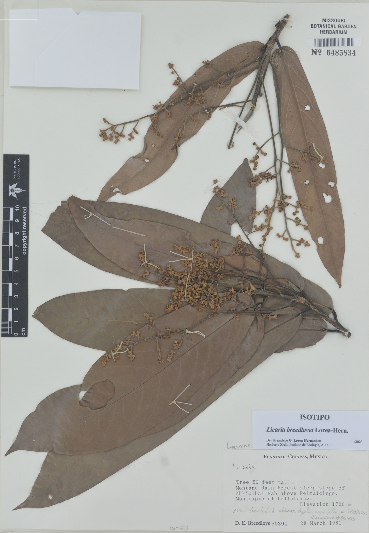
Figure 1. Licaria breedlovei Lorea-Hern. sp. nov., general view.
Paratypes. Costa Rica. Guanacaste: Cantón de Tilarán, San Gerardo Abajo, río Caño Negro, Fincas Quesada y Arce, 10°18’40’’ N, 84°50’02’’ W, 1,100-1,200 m, 5 December 1991, E. Bello & E. Cruz 4262 (XAL). Puntarenas: Cantón de Osa, Rincón, filas al margen izquierdo de Quebrada Vaquedano, 8°38’45’’ N, 83°35’25’’ W, 400 m, 21 July 1990, G. Herrera 4000 (XAL); Cantón de Osa, Aguabuena, cuenca media y superior de Quebrada Orito, Rincón, 8°42’40’’ N, 83°31’40’’ W, 400 m, 25 October 1990, G. Herrera 4510 (MEXU); Cantón de Osa, Rancho Quemado, sector oeste, Sierpe, 8°41’00’’ N, 83°35’40’’ W, 350 m, 25 August 1982, J. Marín & G. Marín 499 (MO, XAL).
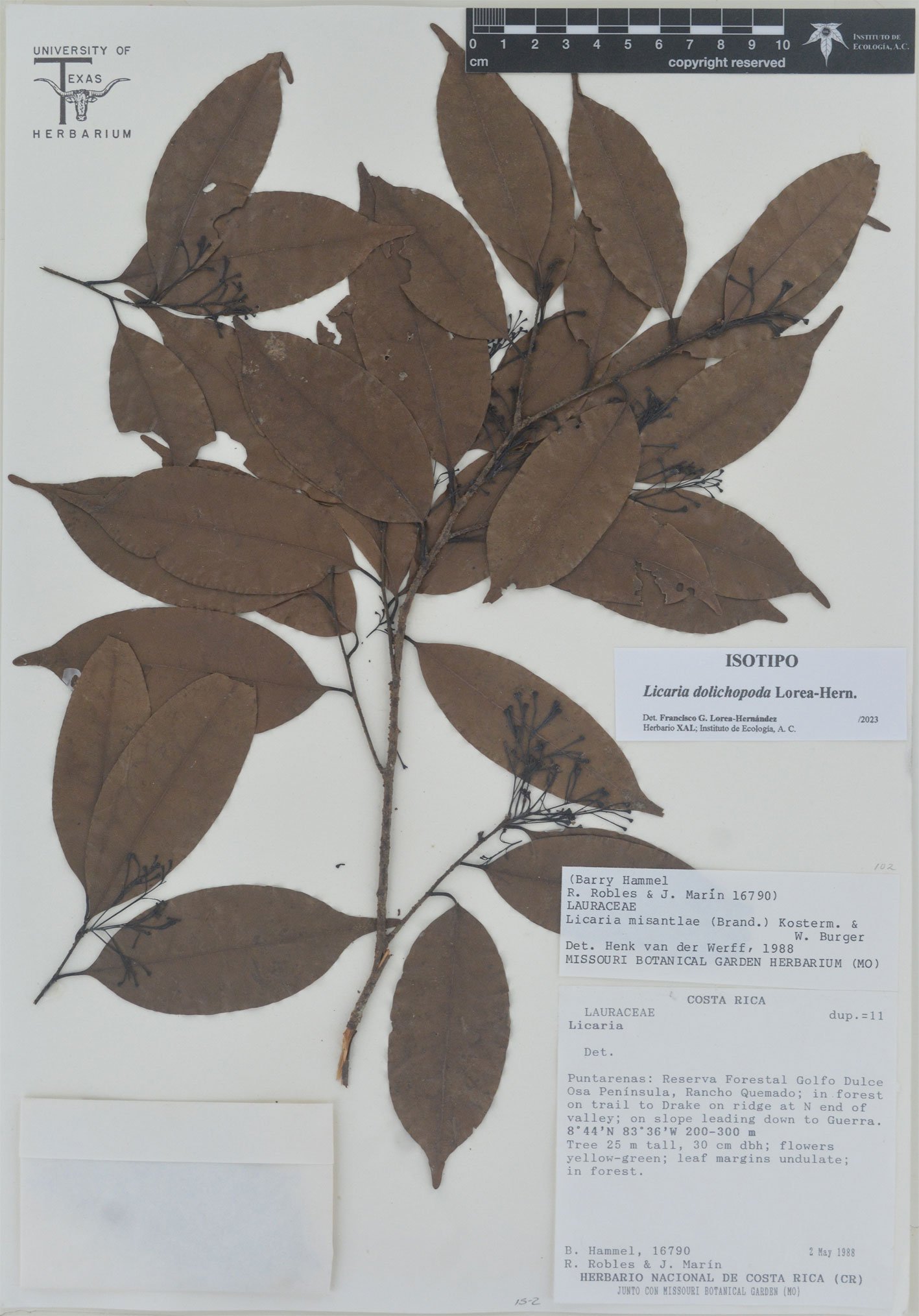
Figure 2. Licaria dolichopoda Lorea-Hern. sp. nov., general view.
Etymology. The name of this species alludes to the distinctive long pedicels that bear the flowers.
Distribution and habitat. Currently the species is known from 2 rather distant areas in Costa Rica that differ in ecological conditions. One of them, in the province of Guanacaste, is located in the Pacific foothills of the southern end of the Sierra de Guanacaste, while the other, in the province of Puntarenas, is in the lowlands of the Peninsula de Osa toward the southeastern extreme of the country. The first one is covered by pre-montane humid forest, and the second by humid tropical forest.
Phenology. Flowering is apparently distributed in 2 peaks: May-July and October-December. Fruits are only known from October.
Conservation status. There is no information about the abundance of the species in the places where it has been collected, neither about the ecological conditions of the vegetation there. However, the distribution range in the southeast is embedded in the Reserva Forestal Golfo Dulce, by the boundaries with the Parque Nacional Corcovado. Thus, there might not be problems with the persistence of the species in that region. The other point of the species distribution is, according to satellite images, within a region with deeply transformed vegetation, although not too far from the Parque Nacional Volcán Arenal, which could hold the species in its flora.
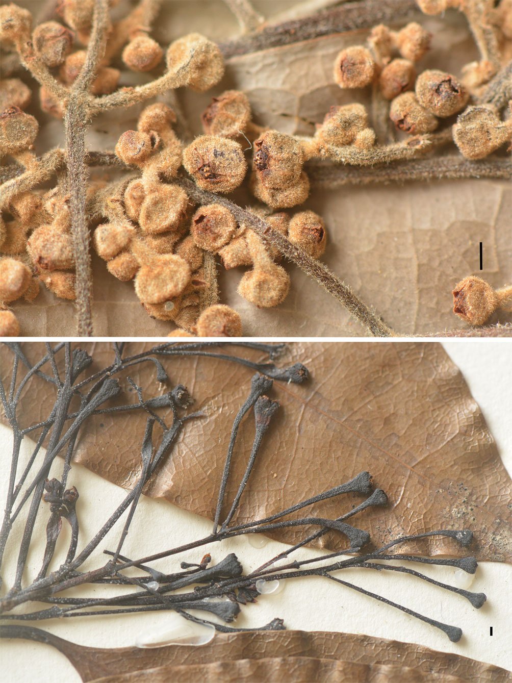
Figure 3. Inflorescence detail of Licaria breedlovei Lorea-Hern. sp. nov. (above), and Licaria dolichopoda Lorea-Hern. sp. nov. (below). Scale bars 1mm.
Remarks
Because of the erect, concave tepals, and extrorse sporangia of stamens in the flowers, L. dolichopoda must be also considered in the subgenus Licaria. The glabrous condition found in every structure of the plant body (stem, leaves, and flowers), as well as the apical openings of stamens, and the lack of staminodes found in this species places it beside L. eurypaniculata (here described), from which it differs in the botryoid architecture of the inflorescence, and the conspicuous caudate leaves. Collection duplicates of L. dolichopoda have been previously distributed as L. cufodontisii Kosterm. (Herrera 4000), and as L. misantlae (Herrera 4510).
Licaria eurypaniculata Lorea-Hern. sp. nov. (Figs. 4, 6)
Diagnosis. Among the species with glabrous leaves, inflexed tepals, lacking staminodes, as well as apical anther openings, this species is distinguished by paniculate inflorescences where the flowers are not aggregate on the floriferous axes, orbicular flowers, tepal surface glabrous abaxially and adaxially, fused stamens throughout, glabrous hypanthium outside and inside, and glabrous pistil.
Trees 6-7 m tall; twigs glabrous, smooth or slightly ribbed, reddish-brown, sparsely lenticellate. Buds glabrous. Leaves alternate, petioles (5.5-)7-9(-10.5) mm long, slightly sulcate above, glabrous, blades (7-)11-16(-19.5) × (2-)3-4.5(-6) cm, narrowly elliptic to lanceolate or elliptic, pinninerved, secondary veins 7-9 pairs, both upper and lower leaf surfaces glabrous, leaf apex acuminate to short caudate, base obtuse to cuneate. Inflorescences 10-11 cm long, apparently terminal, if it is axillary to a bract, this one is inconspicuous, paniculate, basal axes longer than the peduncle, glabrous throughout or sparsely puberulent toward the end of the secondary axes, flowers spaced, not aggregate on the axes, peduncle ca. 3 cm long, pedicels 2-3.2 mm long, glabrous or sparsely puberulent. Flowers spheroidal, greenish, tepals conspicuously inflexed, outer tepals ca. 0.5 × 0.9-1.0 mm, widely ovate to depressed ovate, glabrous abaxially and adaxially, inner tepals ca. 0.4 × 0.6-0.7 mm, ovate or almost orbicular, glabrous abaxially and adaxially, staminodes of whorls I and II absent, stamens of whorl III 0.5-0.6 mm long, fused throughout, filaments glabrous outside, sparsely tomentose inside, anthers ca. 0.1 mm, glabrous, with apical openings, glands ca. 0.1 mm, free, widely elliptic or orbicular, glabrous, hypanthium ca. 0.7 mm deep, glabrous outside, glabrous or sparsely pubescent on the distal section inside, pistil ca. 1.1-1.2 mm long, glabrous throughout, ovary ca. 0.6-0.7 mm long. Fruits (not wholly ripe) 15-17 × 12-12.5 mm, ovoid or ellipsoid, cupule 10-11 × 14-15 mm, crateriform, clearly bimarginate, inner margin 1.1-1.3 mm tall, erect, outer margin 0.5-0.7 mm tall, perpendicular to the inner one, pedicel 3-3.6 × 2-2.2 (at the base) and 3.6-4 (at the apex) mm, obconic.
Taxonomic summary
Type. Panama. Bocas del Toro: along road to Chiriquí Grande, c. 10 road miles from continental divide and about 2 miles along road east of highway, 8°45’ N, 82°15’ W, 300 m, 15 April 1987, G. McPherson 10830 (holotype MO; isotype XAL 124596).
Paratype. Panama. Bocas del Toro: along road to Chiriquí Grande, 10 road-miles from continental divide, ca. 2 road-miles along road east of highway, 8°55’04’’ N, 82°10’04’’ W, 300 m, 9 February 1987, G. McPherson 10453 (MO 5048286).
Etymology. The name of this species alludes to the very long basal secondary axes of the inflorescence, which give a broad triangular profile to the panicle.
Distribution and habitat. The only 2 known collections of the species come from the same area in the Atlantic lowlands of western Panama. No information about the vegetation found at the site was recorded, but considering the geographical factors of the place, it is expected to be tropical rain forest.
Phenology. Flowers in spring, and fruits mature in winter or early spring. The plant is not deciduous.
Conservation status. It seems that the species is not frequent in the area where it was found, for it has been collected only twice. On the other hand, the view of the area from satellite images shows that most of the original vegetation has been cleared; therefore, the species might be endangered.
Remarks
There are no species that come close morphologically to L. eurypaniculata. The other species with a general glabrous condition almost throughout the plant body, L. dolichopoda, is very different, in the shape of the leaves and the structure of the inflorescence. Given the erect, concave tepals, and stamens with extrorse sporangia that L. eurypaniculata presents, it is also a member of the subgenus Licaria.
Licaria gibbitepala Lorea-Hern. sp. nov. (Figs. 5, 6)
Diagnosis. Trees similar to L. excelsa, but distinguished by the obovate to oblanceolate leaves, densely yellowish to orange-brown puberulent inflorescences, tepals with basal half conspicuously swollen, puberulent abaxial surface, sericeous adaxial surface at the base, apically pubescent ovary, and pubescent style.
Trees 15-20 m tall, trunk ca. 25 cm DBH, bark smooth, fragrant; twigs hollow, inhabited by ants, glabrous, sparsely lenticellate, slightly ridged, each ridge originating at one extreme of petiole insertion, acropetal. Buds glabrous or partially pubescent. Leaves alternate, petioles 10-12(-14) mm long, bimarginate above, glabrous, blades (20-)24-30 × (9-)11-13 cm, obovate or oblanceolate, sometimes elliptic, pinninerved, secondary veins (12)14-16 pairs, leaf surface glabrous above and below, leaf apex apiculate, sometimes apiculate-acuminate, leaf base obtuse or rounded. Inflorescences 9-15 cm, seemingly terminal, but actually axillary to tiny, deciduous bracts, on the proximal section of new twigs, paniculate, conspicuously puberulent along all axes, hairs yellowish to orange-brown, peduncle (1-)3.5-4.5 cm, sparsely puberulent, glabrescent, pedicels 2.5-5.5(-7) mm, densely puberulent. Flowers widely obovoid, yellowish-green, fragrant, perianth thick, coriaceous, tepals clearly inflexed, their base conspicuously swollen, outer tepals 1.2-1.4 × 1.6-1.9 mm, widely ovate, puberulent abaxially, sericeous-tomentose at the base and toward the margins adaxially, hairs orange-brown, inner tepals 0.8-1 × 1-1.2 mm, ovate, puberulent abaxially, sericeous-tomentose at the base and tomentose at the middle adaxially, staminodes of whorls I and II absent, stamens of whorl III 0.7-0.8 mm long, fused along their filaments, filaments tomentose at the base outside, tomentose throughout inside, hairs orange-brown, anthers ca. 0.2 mm, free or fused just at the base, glabrous, with apical openings, glands ca. 0.3 mm, only 3 given the fusion of adjoining glands, widely oblong, glabrous, hypanthium 1-1.2 mm deep, obconic, densely puberulent outside, hairs yellowish to orange-brown, sericeous-tomentose inside, hairs reddish-brown, pistil 1.6-1.8 mm long, top of the ovary and style pubescent, ovary 0.8-1.2 mm long. Fruits (nearly ripe) 19-23 × 15.5-16.5 mm, ellipsoid, cupule ca. 16.5 × 18.5 mm, cotyliform, sparsely lenticellate, seemingly tri-margined, the 2 regular margins plus the swollen projections of the tepals, inner margin ca. 1.6 mm tall, erect, outer margin 2.2-2.5 mm tall, erect, pedicel 4.5-7 mm long, continuous with the base of the cupule, 3.5 mm diam. at the base.
Taxonomic summary
Type. Costa Rica. Limón: Reserva Biológica Hitoy Cerere, 300 m aguas abajo de la confluencia del río Hitoy con el río Cerere, margen izquierda por la fila que lleva al cerro Bobócora, 9°39’00’’ N, 83°02’45’’ W, 200 m, 20 February 1989, G. Herrera & A. Chacón 2427 (holotype MO, isotype XAL 124445).
Etymology. The name is derived from the conspicuous swollen condition of the base of the tepals; the feature is distinctive.
Distribution and habitat. So far, this species is known only from the southwestern end of Costa Rica. Although no information about the habitat was recorded, there is no doubt that the place lies within the tropical rain forest territory.
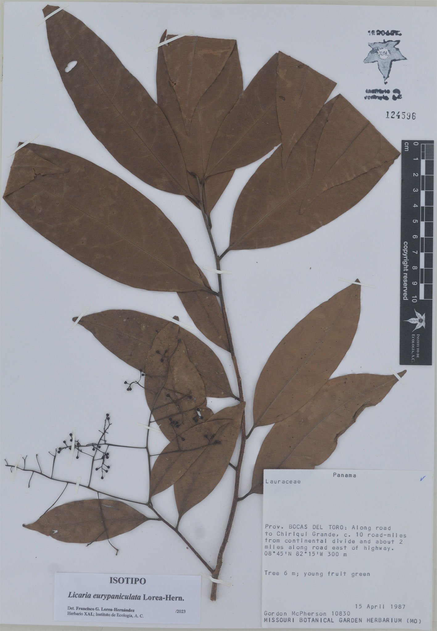
Figure 4. Licaria eurypaniculata Lorea-Hern. sp. nov., general view.
Phenology. With flowers and ripe fruits around the end of winter. The species has perennial leaves.
Conservation status. There is no information about the abundance or extent of distribution of the species, but as it is known to grow in the grounds of a nature reserve, it can be expected that it is not under high risk of extinction but certainly endangered.
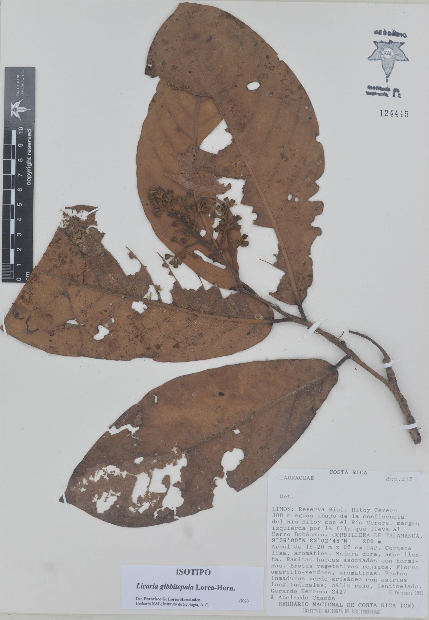
Figure 5. Licaria gibbitepala Lorea-Hern. sp. nov., general view.
Remarks
Licaria gibbitepala seems to be closely related to L. tomentulosa and, at the same time, to the group of species around L. excelsa. All of them have ridged twigs, large leaves, flowers with erect, concave tepals, no staminodes, and sporangia with apical openings. The hollow twigs, along with the obovate to oblanceolate leaves, and the conspicuous gibbous base of the tepals distinguish L. gibbitepala.
Licaria gracilis Lorea-Hern. sp. nov. (Figs. 7, 9)
Diagnosis. Small trees with glabrous leaves, botryoid, few-flowered inflorescences, glabrous, erect tepals, lacking staminodes, free stamens, anther openings elliptic, lateral, strongly oblique, glands present, glabrous hypanthium outside and inside, glabrous pistil.
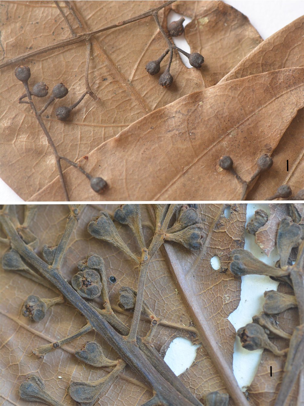
Figure 6. Inflorescence detail of Licaria eurypaniculata Lorea-Hern. sp. nov. (above), and Licaria gibbitepala Lorea-Hern. sp. nov. (below). Scale bars 1mm.
Trees to 6 m tall; twigs smooth, dark brown to reddish brown, pruinose, puberulent, glabrescent, sparsely lenticellate. Buds glabrous. Leaves alternate, petioles (4-)8-11 mm long, puberulent, soon glabrous, canaliculate above, blades 8.5-13 × 3.5-5.5 cm, elliptic or narrowly elliptic, pinninerved, secondary veins 5-7 pairs, leaf surface glabrous above and below, but the lower surface puberulent in the beginning, leaf apex caudate, sometimes just acuminate, base obtuse to cuneate. Inflorescences 2.5-3.5 cm long, axillary to leaves and to tiny, deciduous bracts, on the proximal section of new twigs, botryoid, racemiform, few-flowered (less than 10 flowers), glabrous throughout or with some hairs toward the end of the peduncle, peduncle 1.8-2 cm long, pedicels 3-4.5 mm long, glabrous. Flowers obovoid, pale yellow, tepals erect to slightly inflexed, concave, outer tepals ca. 0.8 × 1.3 mm, very widely ovate to depressed ovate, glabrous abaxially, with some long, appressed hairs ascending from the base adaxially, inner tepals ca. 0.5 × 0.8 mm, ovate or widely ovate, glabrous abaxially, adaxially like the outer tepals, staminodes of whorls I and II absent, stamens of whorl III ca. 0.7 mm long, free, but very close one to each other, widely ovate in outline, filaments sparsely tomentulose outside and inside, anthers ca. 0.4 mm, tomentulose at the base outside, tomentulose inside along the central line, openings lateral, oblique, glands ca. 0.4 mm, rounded, glabrous, hypanthium ca. 0.7 mm deep, obconic, glabrous inside and outside, pistil ca. 1.7 mm long, glabrous, ovary ca. 0.8 mm long. Fruit unknown.
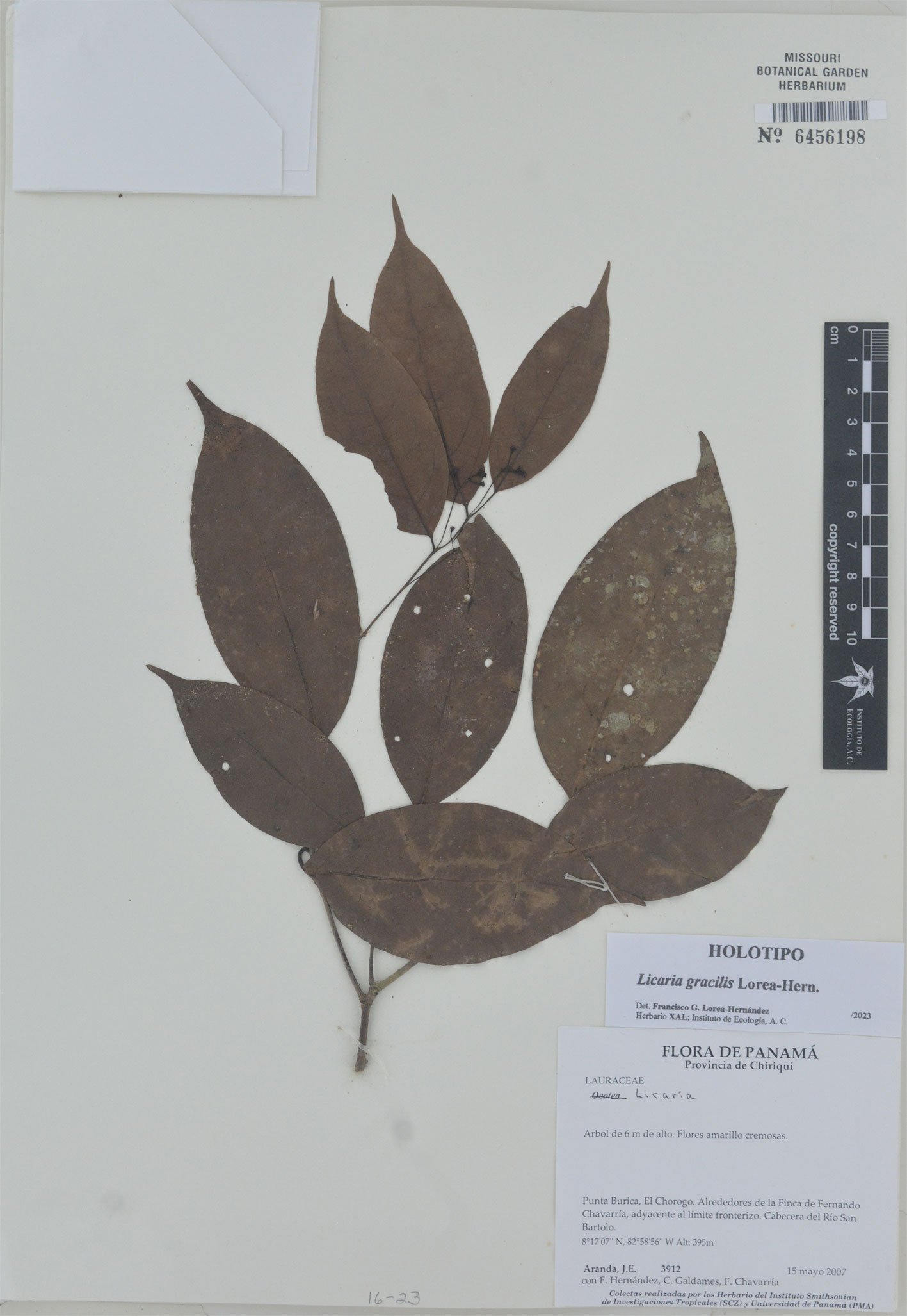
Figure 7. Licaria gracilis Lorea-Hern. sp. nov., general view.
Taxonomic summary
Type. Panama. Chiriquí: Punta Burica, El Chorogo, alrededores de la finca de Fernando Chavarría, adyacente al límite fronterizo, cabecera del río San Bartolo, 8°17’07’’ N, 82°58’56’’ W, 395 m, 15 May 2007, J. E. Aranda et al. 3912 (holotype MO 6456198).
Etymology. The name of the species is derived from the attractive view that the slender inflorescences give to the plant.
Distribution and habitat. The species is known only from the location where it was first and last collected. No information about the habitat is mentioned in the data-label of the specimen, except that was collected nearby a ranch. The original vegetation must have been tropical evergreen forest or semi-evergreen forest.
Phenology. Flowers during spring; ripe fruits expected during winter or early spring, since maturation of fruits in most Lauraceae takes around a year after flowering.
Conservation status. The species might be (critically) endangered, for most of the land in the area where it was collected has been transformed for diverse agricultural purposes.
Remarks
The few-flowered, botryoid inflorescence, tiny flowers, and very oblique, lateral openings of the sporangia distinguish this species straightaway. There is no species whose general morphology indicates association with L. gracilis. The singular way that the openings of the stamens are displayed resemble that found in Licaria cogolloi van der Werff, and L. caribaea Gómez-Lau. & Cascante, but besides this, there is no other feature that might suggest a relationship to those species. For the features of its flowers, Licaria gracilis belongs to subgenus Licaria.
Licaria minutiflora Lorea-Hern. sp. nov. (Figs. 8, 9)
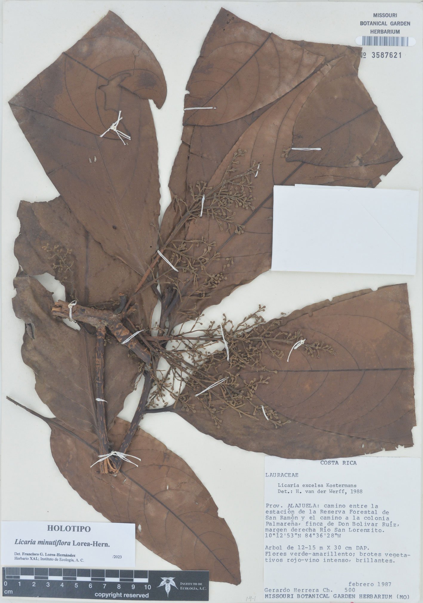
Figure 8. Licaria minutiflora Lorea-Hern. sp. nov., general view.
Diagnosis. Trees similar to L. pergamentacea, but distinct by the presence of hollow twigs, glabrous buds, abaxially densely tomentulose tepals, internally pubescent hypanthium, apically pubescent ovary, and pubescent style.
Trees up to 20 m tall, trunk ca. 30 cm DBH; twigs hollow, inhabited by ants, glabrous, smooth or slightly ridged, each ridge originates at one extreme of petiole insertion, acropetal, sparsely lenticellate. Buds glabrous. Leaves alternate, petioles (7-)15-20(-30) mm, glabrous, bimarginate above, blades (11-)20-28(-34.5) × (3-)5-9(-13) cm, narrowly elliptic or narrowly ovate, pinninerved, secondary veins 9-12 pairs, leaf surface glabrous on both sides, leaf apex acute, slightly apiculate, base acute or obtuse. Inflorescences (6-)9-12(-15) cm long, axillary to tiny, deciduous bracts, on the proximal section of new twigs or axillary to leaves, paniculate, tomentulose, peduncle (0.5-)1.5-3(-4) cm long, pedicels (1.2-)2.5-4(-6) mm long, densely tomentulose. Flowers obovoid or ellipsoid, yellowish-green, tepals inflexed, outer tepals 0.5-0.8 × 0.8-1 mm, widely ovate, densely tomentulose abaxially, tepal surface concealed or almost so by hairs, glabrous adaxially, inner tepals 0.5-0.7 × 0.5-0.6 mm, ovate, densely tomentulose abaxially, glabrous adaxially, staminodes of whorls I and II absent, stamens of whorl III 0.5-0.6 mm long, free or barely united by filament base, filaments tomentose at base outside, glabrous or sparsely pubescent along the medial line inside, anthers ca. 0.2 mm, glabrous, openings apical, glands ca. 0.2 mm, free, rounded, hypanthium 0.6-0.8 mm deep, obconic, densely tomentulose outside, sericeous on upper half inside, hairs yellowish or reddish, pistil ca. 1.4 mm long, top of the ovary and style pubescent, ovary 0.8-1 mm long. Fruits ca. 19.5 × 15-16.5 mm, ellipsoid, cupule 15-16 × 18-20 mm, urceolate, lenticellate, conspicuously bimarginate, inner margin 1.2-1.5 mm tall, outer margin 1-1.2 mm, extended, pedicel 6.5-9 mm long, continuous with the cupule, 2.8-3.6 mm diameter at base.
Taxonomic summary
Type. Costa Rica. Alajuela: camino entre la estación de la Reserva Forestal de San Ramón y el camino a la colonia Palmareña, finca de don Bolívar Ruiz, margen derecha río San Lorencito, 10°12’53’’ N, 84°36’28’’ W, February 1987, G. Herrera 500 (holotype MO 3587621; isotypes MEXU 638804, TEX).
Paratypes. Costa Rica. Alajuela: Reserva Biológica Monteverde, Poco Sol, La Cutacha de San Bosco, 10°22’ N, 84°40’ W, 900 m, 1 April 1989, E. Bello 784 (MEXU 1304162; MO 6142952; XAL 124442); Bosque Eterno de los Niños, Reserva de Arenal, río Peñas Blancas, Quebrada Agua Gata, Finca Villalobos, 10°23’ N, 84°42’ W, 1,000 m, 20 April 1990, E. Bello 2208 (MO 6130824; XAL 124446); Cantón de Upala, Colonia La Libertad, 10°52’ N, 85°17’ W, 300 m, 3 August 1991, Q. Jiménez & G. Rivera 1011 (MO 6117397; XAL 124597). Guanacaste: Parque Nacional Guanacaste, Estación Pitilla, 10°00’15’’ N, 85°25.2’ W, 500 m, 27 May 1989, G. Herrera et al. 2942 (MO; XAL 124428).
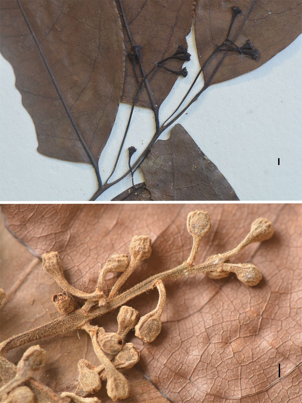
Figure 9. Inflorescence detail of Licaria gracilis Lorea-Hern. sp. nov. (above), and Licaria minutiflora Lorea-Hern. sp. nov. (below). Scale bars 1 mm.
Etymology. The very small flowers, whose tepals are less than 1 mm long, is the feature on which the species name is based.
Distribution and habitat. This species is known from the northern hills of the Cordillera de Guanacaste (Guanacaste Mountain Range) and the western part of the Cordillera Central (Central Mountain Range), between 200 and1,000 m asl. Prevailing vegetation in the region is tropical evergreen forest and montane rain forest. The species has been collected also in pasture fields. There is a fruiting specimen from the Osa Peninsula (Hammel et al. 16984) that seems to belong to L. minutiflora but until confirmed with a flowering specimen, the presence of the species in this part of the country remains uncertain.
Phenology. Flowers toward the end of winter and early spring; fruits must be ripe around the end of autumn or early winter.
Conservation status. Most specimens of this species have been collected within nature reserves. Therefore, it is considered not threatened, even though its abundance is still unknown.
Remarks
As has been mentioned elsewhere in this paper, Licaria minutiflora is part of the L. excelsa species group. Its general appearance resembles that of L. pergamentacea, for the size and shape of the leaves, structure and hairiness of the inflorescence, and for having small oblong-ellipsoid, not coriaceous flowers. However, besides the presence of hollow twigs, it differs by having flowers with the upper part of the hypanthium homogeneously pubescent inside, and a pubescent pistil.
Licaria ochracea Lorea-Hern. sp. nov. (Figs. 10, 12)
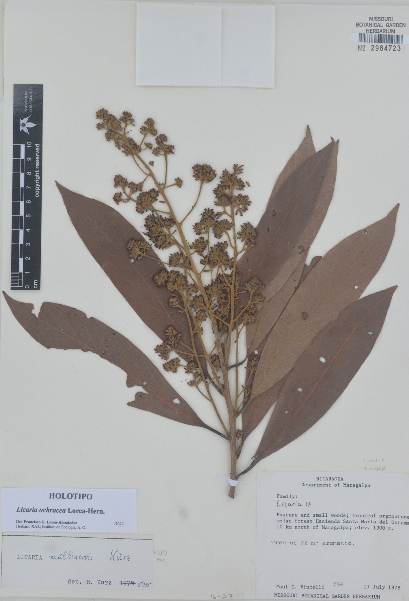
Figure 10. Licaria ochracea Lorea-Hern. sp. nov., general view.
Diagnosis. Trees similar to L. multinervis H. W. Kurz, but differing by lower surface indument of leaves composed by 2 types of hairs, the most numerous tomentulose, the fewer sericeous, long inflorescences, terminal or axillary to leaves, with rachis up to 15 cm, fully exserted anthers, clearly stalked glands, conspicuous hypanthium tube projected beyond the insertion point of stamens.
Trees up to 22 m tall, twigs smooth, densely tomentose, hairs initially yellowish-brown, then greysh, sparsely and inconspicuously lenticellate. Buds tomentose. Leaves alternate, petioles (10-)15-20 mm long, tomentose, glabrescent, channeled above, blades 12.5-18.5 × (2.5)3.5-4.5 cm, narrowly elliptic, sometimes narrowly oblanceolate, pinninerved, secondary veins (9)10-13 pairs, leaf surface glabrous above, tomentose below, most hairs sinuous, rather appressed, or patent, fewer hairs straight, appressed, leaf apex acuminate, base narrowly cuneate. Inflorescences (7-)10-18 cm long, axillary to leaves, less frequently terminal, paniculate, densely tomentose, hairs like on twigs, flowers agglomerate at the end of terminal axes, peduncle 0.2-1.5(-3.5) cm long, pedicels (1-)1.5-2 mm long, tomentose. Flowers narrowly oblong, tepals erect, concave, outer tepals, 1-1.3(-1.5) × (1-)1.1-1.3 mm, widely ovate, tomentose abaxially, glabrous adaxially, except for a few long, appressed hairs, coming from the base, inner tepals 1-1.1(-1.4) × 0.8-0.9 mm, ovate, with a pattern of pubescence similar to that of outer tepals, staminodes of whorls I and II absent, stamens of whorl III 3-3.3(-3.8) mm long, coherent along their filaments or even at the base of the anthers, easily separable, filaments tomentose on both faces, anthers 0.9-1.1 mm long, free or coherent at the base, glabrous, completely exserted, openings dorsolateral, glands 0.7-0.8 mm, free, oblanceolate, glabrous, clearly stalked, stalk pubescent, hypanthium 1.2-1.3(-1.6) mm deep, extended 0.3 mm beyond the insertion point of stamens, tomentose outside, densely hirsute-tomentose inside, hairs golden-brown, pistil 3.6-3.9 mm long, sparsely pubescent, at least some hairs on the upper half of the ovary and lower half of the style, ovary 0.9-1.1 mm long. Fruits unknown.
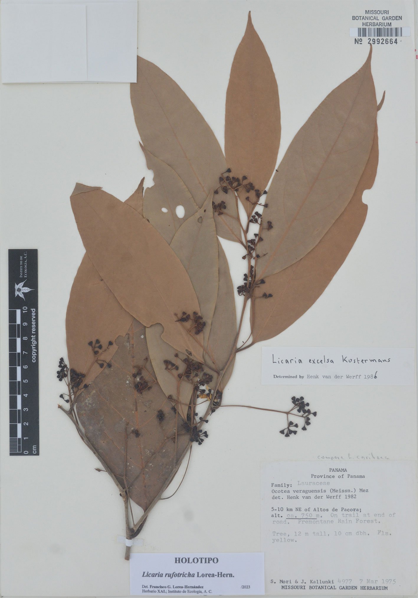
Figure 11. Licaria rufotricha Lorea-Hern. sp. nov., general view.
Taxonomic summary
Type. Nicaragua. Matagalpa (according to current maps it should be Jinotega): pasture and small woods, tropical premontane forest, Hacienda Santa María del Ostuma, 10 km N of Matagalpa, 1,300 m, 17 July 1978, P. C. Vincelli 756 (holotype MO 2984723; isotypes LL, MEXU 691292).
Etymology. The name refers to the conspicuous orange-brown pubescence of the species on young twigs and main axes of inflorescences.
Distribution and habitat. Only known from the place of type collection, where the Cordillera Isabelia and Cordillera Dariense meet.
Phenology. Flowers in summer; fruit season is not known, but since it has been observed that maturation of fruits in most Lauraceae takes around a year after flowering, possibly ripe fruits are present during spring or early summer.
Conservation status. There is no certainty on the conditions that might be affecting the survival of the species. The type was collected in a private property that used to be preserved for ecotourism activities, but its current situation is unknown. However, since the species has not been collected again, it is suspected to be endangered.
Remarks
The collection on which the description of this species is based was initially identified by Kurz (2000) as L. multinervis; actually it is cited as a paratype of this species. But the impression of being conspecific with this taxon disappears with a detailed survey of the morphology. Important differences are the pubescence on the lower surface of the leaves (simple in L. multinervis vs. made of 2 types of hairs in L. ochracea), position of the inflorescences (axillary to small bracts in the proximal section of new branches in L. multinervis vs. axillary to leaves or terminal in L. ochracea), length of inflorescences (up to 3.5 cm long in L. multinervis vs. 5-7 times longer in L. ochracea), protrusion of anthers (partially exserted in L. multinervis vs. fully exerted in L. ochracea), and projection of hypanthium tube beyond the insertion point of stamens (short in L. multinervis vs. conspicuous in L. ochracea). However, L. multinervis and L. ochracea seem to be more closely related to each other than to the rest of species in the area that present fully exserted stamens, namely L. agglomerata van der Werff, L. capitata (Schltdl. et Cham.) Kosterm., L. nitida van der Werff, and L. vanderwerffii (here described).
Licaria rufotricha Lorea-Hern. sp. nov. (Figs. 11, 12)
Diagnosis. Small trees, distinct for the conspicuously obovoid flowers, aggregate toward the end of the secondary floriferous axes, with inflexed tepals, glabrous abaxially, reddish-brown hirsute-sericeous adaxially, lacking staminodes, stamens fused throughout, reddish-brown hirsute, anther openings apical, hypanthium mostly glabrous outside, reddish-brown hirsute inside, and ovary distally pubescent.
Trees to 12 m tall; twigs smooth or inconspicuously ridged, each ridge originating at one extreme of petiole insertion, acropetal, lenticellate, grayish, densely puberulent, glabrescent. Buds glabrous. Leaves alternate, petioles 10-13 (-17) mm long, slightly channeled above, puberulent, blades (14.5-)16.5-20(-23) × 4-5.5(-9) cm, elliptic or narrowly elliptic, pinninerved, secondary veins 6-7 pairs, leaf surface densely puberulent above when young, glabrescent, rather persistently puberulent below, leaf apex acuminate, base cuneate, sometimes obtuse or narrowly cuneate to indistinctly attenuate. Inflorescences (3-)5-8(-10.5) cm, axillary to tiny, deciduous bracts, on the proximal section of new twigs, or axillary to new leaves, paniculate, flowers aggregate at the end of secondary axes, densely puberulent on peduncle and rachis, glabrate toward the ultimate axes, peduncle (2-)3.5-5.5(-7.5) cm long, pedicels 2-3.5(-4.5) mm long, glabrous or sparsely puberulent. Flowers obovoid or obconic, pale yellow, tepals conspicuously inflexed, outer tepals 1-1.2 × 2-2.4 mm, widely ovate, glabrous abaxially, hirsute-sericeous adaxially, hairs reddish-brown, inner tepals 0.8-1 × 0.8-0.9 mm, ovate or elliptic, glabrous abaxially, generally mostly hirsute adaxially, hairs reddish-brown, surpassing the apical margin of the tepals, making them appear fimbriate, staminodes of whorls I and II absent, stamens of whorl III, 0.6-0.7 mm long, fused throughout, filaments hirsute on both faces, hairs reddish-brown, anthers ca. 0.2 mm, pubescent, except around the margin of the openings, hairs like those of the filaments, glands ca. 0.4 mm, free, rounded or oblate, glabrous, hypanthium 0.8-0.9 mm deep, glabrous or sparsely puberulent outside, hirsute inside, hairs like those of the filaments, pistil 1.7-2 mm long, ovary ca. 0.8 mm long, sparsely pubescent distally, hairs whitish. Fruits unknown.
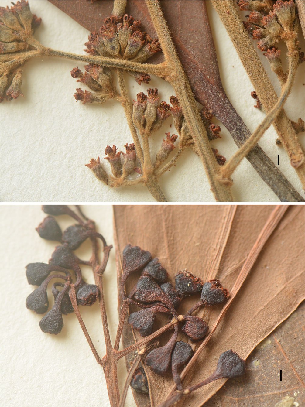
Figure 12. Inflorescence detail of Licaria ochracea Lorea-Hern. sp. nov. (above), and Licaria rufotricha Lorea-Hern. sp. nov. (below). Scale bars 1 mm.
Taxonomic summary
Type. Panama. Panama: 5-10 km NE of Altos de Pacora, on trail at end of road, ca. 750 m, 7 March 1975, S. Mori & J. Kallunki 4977 (holotype MO 2992664).
Etymology. The name given to this species refers to the dense red-brown pubescence in the interior of the flowers, covering the adaxial surface of tepals, stamen filaments, anthers, and hypanthium inside.
Distribution and habitat. Just known from the place where the type was collected (around 25-30 km NE of Panama City), with tropical evergreen forest or semi-evergreen forest as original vegetation.
Phenology. Flowers around the end of winter or early spring; ripe fruits expected during winter, since maturation of fruits in most Lauraceae takes around a year after flowering.
Conservation status. Probably the species is endangered. Most of the vegetation in the surroundings of the place where the species was collected has been cut down for cattle raising or agricultural purposes. But the southern boundary of the Parque Nacional Chagres (Chagres National Park) is very close to that place, and the Nature Reserve Cocobolo is a few kilometers ENE of it as well. So, even it has not been collected again, it is hoped the species is still around there.
Remarks
There is no other species in the Mesoamerican area with the distinctive reddish-brown pubescence found in the interior of the Licaria rufotricha flowers. Yellowish to reddish-brown pubescence is present on the filaments of stamens and/or inside the hypanthium of several species, like L. agglomerata, L. excelsa, L. gibbitepala, and L. tomentulosa, but it is never found on the tepals surface. In fact, its general morphology does not suggest a relation to any species in the region.
Licaria sarukhanii Lorea-Hern. sp. nov. (Figs. 13, 15)
Diagnosis. Trees similar to L. alata, but differing by terminal, subsessile inflorescences, longer pedicels (up to 10.5 mm), flowers widely ellipsoid, abaxial tepal surface tomentose at the base and papillose toward the apex, hypanthium densely tomentose outside, sericeous-tomentose inside, and style pubescent.
Trees to 20 m tall, twigs glabrous, grayish to grayish-brown, slightly ridged, each ridge originating at one extreme of petiole insertion, acropetal, sparsely lenticellate. Buds glabrous or pubescent at the apex of the bud scales. Leaves alternate, petioles (11-)13-17(-20) mm long, slightly bimarginate, glabrous, blades (12.5-)20-32(-37) × (5-)7-10(11.5) cm, narrowly elliptic, occasionally oblanceolate, pinninerved, secondary veins (12)14-18 pairs, leaf surface glabrous on both sides, leaf apex acuminate, sometimes acute, base obtuse or acute. Inflorescences 12-22 cm long, terminal, paniculate, tomentose, soon glabrescent, hairs patent or oblique, grey or yellowish-grey, peduncle 0.2-0.4 cm long, pedicels (3-)5-8(-10.5) mm long, glabrous or sparsely tomentose. Flowers broadly ellipsoid, pale green, tepals inflexed, outer tepals 0.8-0.9 × 1.8-2 mm, very widely ovate, concave, tomentose over the basal half, and papillose-pubescent over the distal half abaxially, glabrous or with few straight hairs at base adaxially, inner tepals 0.7-0.9 × 0.4-0.8 mm, ovate, pubescence pattern abaxially like that of outer tepals, but less papillose, glabrous adaxially, staminodes of whorls I and II absent, stamens of whorl III 0.7-0.9 mm long, fused along their filaments, filaments tomentose along the central line on both faces, anthers 0.2-0.4 mm long, glabrous, openings apical, glands ca. 0.4 mm, oblong, flattened, frequently reduced or absent, glabrous or tomentose on the base abaxially, hypanthium ca. 1 mm deep, densely tomentose outside, hairs sinuous, sericeous-tomentose inside, pistil 1.3-1.6 mm long, ovary 0.8-1.2 mm long, glabrous, style rather densely pubescent. Fruits 27-30 × 17-18 mm, ellipsoid, cupule 15-17.5 × 18-19.5 mm, urceolate, bimarginate, but the margins barely discernible, ca. 0.5 mm, erect, pedicel 4-5 × 3.5-4.5 mm.
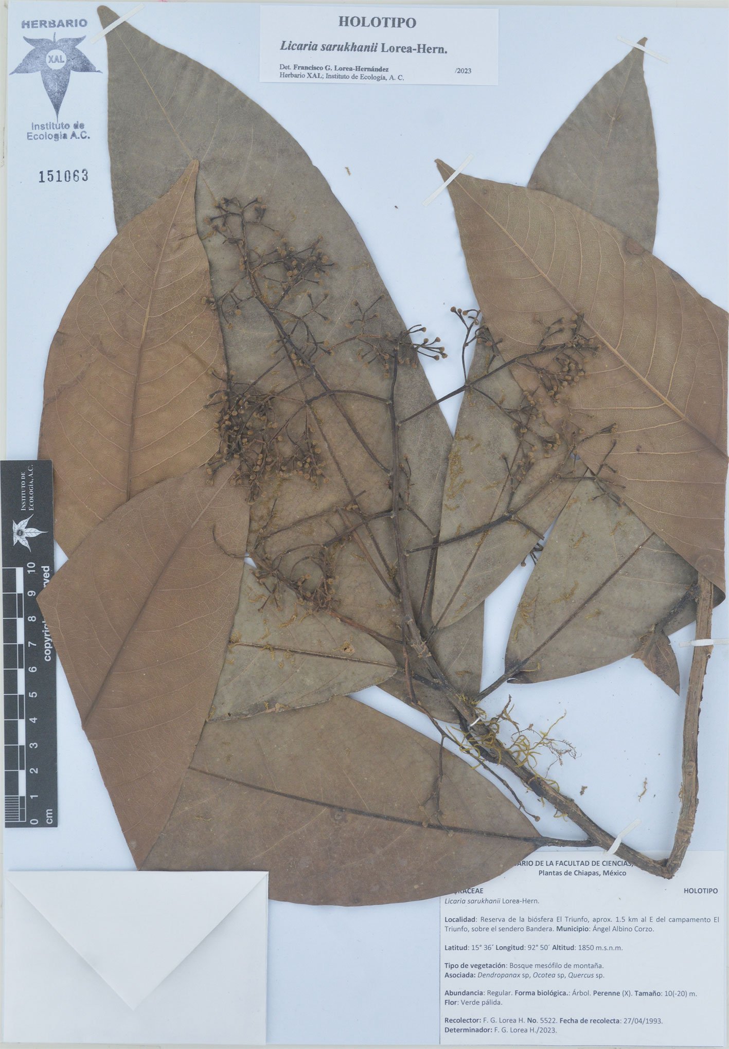
Figure 13. Licaria sarukhanii Lorea-Hern. sp. nov., general view.
Taxonomic summary
Type. Mexico. Chiapas: municipio de Ángel Albino Corzo, Reserva de la Biosfera El Triunfo, aprox. 1.5 km al E de Campamento El Triunfo, sobre el Sendero Bandera, 15°36’ N, 92°50’ W, 1,850 m, 27 April 1993, F. Lorea 5522 (holotype XAL 151063; isotypes [to be distributed]).
Paratypes. Mexico. Chiapas: municipio de Ángel Albino Corzo, Polígono I de la Reserva de la Biosfera El Triunfo, 15°39’ N, 92°48’ W, 1,900 m, 21 February 1993, S. Solórzano 67 (MEXU 754117); Reserva El Triunfo, camino a Cerro de la Bandera, 25 March 1986, M. L. Ávila and V. H. Hernández s/n (MEXU 877857, TEX 146383); Reserva de la Biosfera El Triunfo, sendero Palo Gordo, 15°40’10’’ N, 92°48’42’’ W, 1,990 m, 22 March 2006, F. González-García s/n (XAL 113841).
Etymology. The species is dedicated to José Sarukhán, a Mexican plant ecologist who has played an important role in making a huge amount of information about Mexico’s biodiversity, ecosystem conservation, and sustainable development accessible to the public.
Distribution and habitat. So far, the species is known only from the central region of the Sierra Madre de Chiapas, from 1,800 to 2,000 m asl where the montane rain forest is the dominant type of vegetation.
Phenology. Flowers toward the end of winter and early spring; ripe fruits were found in the same interval of time.
Conservation status. All the collections of the species come from the nature reserve El Triunfo, located in the Sierra Madre de Chiapas, which has persisted largely undisturbed for its almost forty years of existence. Thus, considering the size of the area covered with montane rain forest in the reserve, the species might be regarded as vulnerable.
Remarks
Licaria sarukhanii is part of the L. excelsa species group, with a closer relation to L. breedlovei, because they share tomentose inflorescences and flowers rather widely ellipsoid to obloid. They differ by the conduplicate leaf bases, sparsely sericeous lower leaf surface, conspicuously pedunculate inflorescences axillary to small bracts or leaves, fused anthers, and style sparsely pubescent present in L. breedlovei, in contrast to flat leaf base, glabrous lower leaf surface, terminal, sub-sessile inflorescences, free anthers, and conspicuously pubescent style in L. sarukhanii.
Licaria tomentulosa Lorea-Hern. sp. nov. (Figs. 14, 15)
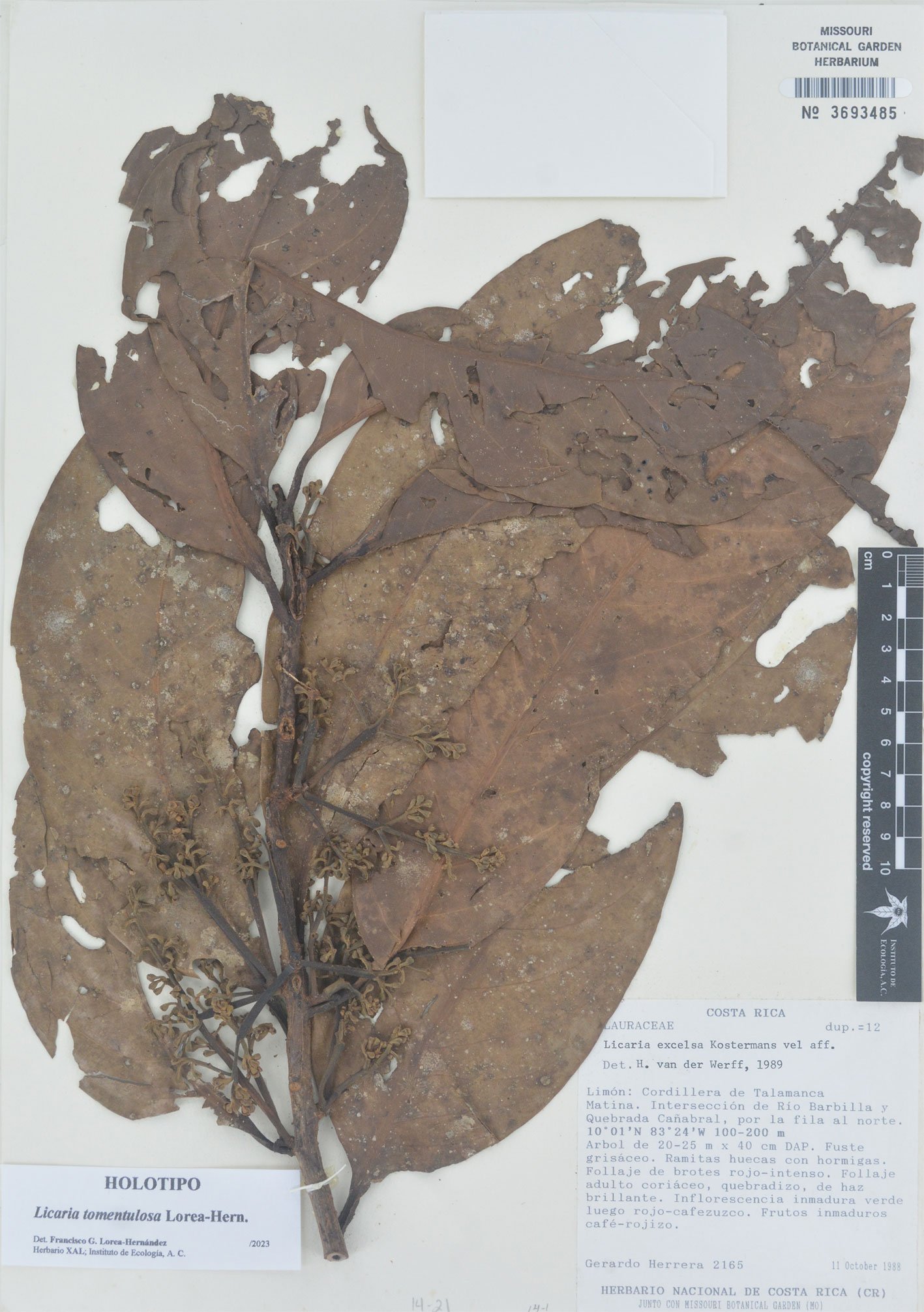
Figure 14. Licaria tomentulosa Lorea-Hern. sp. nov., general view.
Diagnosis. Trees similar to L. excelsa, but distinguished by presenting hollow twigs, inflorescences yellowish-brown tomentulose, flowers conspicuously obovoid, tepals densely tomentulose abaxially, and apex of the ovary and style conspicuously pubescent.
Trees up to 25 m tall, and trunk 50 cm DBH, twigs hollow, inhabited by ants, smooth or slightly ridged, glabrous, grayish-brown, sparsely lenticellate. Buds glabrous. Leaves alternate, petioles (14-)17-22(-24) mm long, bimarginate above, glabrous, blades (22-)25-30(-34) × (6-)8-10(-12) cm, narrowly elliptic or elliptic, pinninerved, secondary veins (9)11-13 pairs, leaf surface glabrous on both sides, leaf apex acute or short acuminate, base obtuse, rounded or shortly attenuate, particularly in leaves close to the twig tips. Inflorescences 6.5-9.5(13.5) cm long, axillary to tiny, deciduous bracts, on very short branches axillary to leaves, paniculate, tomentulose, hairs yellowish-brown, peduncle 2.5-4 cm long, pedicels (1-)2-3.5 mm long, densely tomentulose. Flowers obovoid, thick, coriaceous, greenish-yellow, tepals inflexed, concave, outer tepals 0.7-1 × 1.4-1.7 mm, widely ovate, densely tomentulose abaxially, hairs almost concealing the surface, marginal tomentose bands and some long, appressed hairs at the base adaxially, inner tepals 0.6-0.9 × 0.8-0.9 mm, ovate, sometimes slightly conduplicate, densely tomentulose abaxially, pattern of pubescence adaxially like in the outer tepals, staminodes of whorls I and II absent, stamens of whorl III 0.8-1.1 mm long, fused throughout, filaments tomentose outside on lower half, densely tomentose all over the inner face, hairs reddish-brown, anthers ca. 0.2 mm, glabrous outside, densely tomentose inside, openings apical, glands 0.3-0.4 mm, frequently fused between adyacent stamens, transversely oblong, oblong when free, hypanthium 1-1.2 mm deep, densely tomentulose outside, tomentulose inside, sometimes only in the upper half, hairs mainly reddish-brown, pistil 2-2.3 mm long, ovary 1.1-1.4 mm long, apex of the ovary and style conspicuously pubescent. Fruits (not fully ripe) ca. 13 × 13 mm, spheroidal, cupule 13-14 × 17-18 mm, crateriform, lenticellate, bimarginate, inner margin 0.7-1 mm tall, erect, outer margin 0.5-0.7 mm, erect to spreading, pedicel 4-6 × 3-4 (apex) and 2 mm (base).
Taxonomic summary
Type. Costa Rica. Limón: Cordillera de Talamanca, Matina, intersección de río Barbilla y quebrada Cañabral, por la fila al norte, 10°01’ N, 83°24’ W, 100-200 m, 11 October 1988, G. Herrera 2165 (holotype MO 3693485; isotypes MEXU 529888, 529889, 717774, and 718334; TEX).
Paratypes. Costa Rica. Alajuela: Upala, Bijagua, El Pilón, Cerro La Carmela, entre río Celeste y cabeceras del río Chimurria, 10°43’15’’ N, 84°59’45’’ W, 1,000 m, 11 July 1988, G. Herrera 2056 (MEXU 529875, 717781; MO 3693486; US 3655515). Limón: Reserva Biológica Hitoy Cerere, Valle de la Estrella, sendero a Cerro Bobócara, 9°41’00’’ N, 83°04’20’’ W, 798 m, 17 August 1990, G. Herrera 4115 (MEXU 1304090; MO 6142953; XAL 124444); Reserva Indígena Talamanca, camino a Soki entre la Quebrada Amubri, margen izquierda de río Lari, 9°29’40’’ N, 82°89’40’’ W, 200 m, 29 June 1989, A. Chacón 25 (MO; XAL 124437).
Etymology. The name is for the abundant tomentulose pubescence that covers the axes of the inflorescence, as well as the abaxial surface of tepals and hypanthium.
Distribution and habitat. Known only from Costa Rica, along the Atlantic lowlands adjacent to the Sierra de Talamanca, and the Sierra de Guanacaste. Tropical rain forest used to be the predominant vegetation there, but currently a big amount of land has been changed to agricultural activities or other affairs.
Phenology. Flowers in summer and early autumn; ripe fruits in summer.
Conservation status. Given the deterioration of the habitat, the species might be considered vulnerable or endangered, in spite of its wide range of distribution.
Remarks
Licaria excelsa and L. tomentulosa are much alike. Considering the available material, distinguishing characters seem to work well to separate both species; hollow twigs, as well as type and distribution of pubescence on vegetative and floral parts, are consistently present in all the specimens considered as L. tomentulosa, making it a clear morphological unit, distinct from L. excelsa.
Licaria vanderwerffii Lorea-Hern. sp. nov. (Figs. 16, 17)
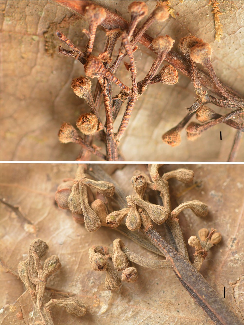
Figure 15. Inflorescence detail of Licaria sarukhanii Lorea-Hern. sp. nov. (above), and Licaria tomentulosa Lorea-Hern. sp. nov. (below). Scale bars 1 mm.
Diagnosis. Similar to L. agglomerata, but different by the free stamens, white pubescence of stamens, hypanthium densely white tomentose inside, and pistil glabrous.
Shrubs or small trees 1-3 m tall, twigs hollow, smooth, sparsely lenticellate, glabrous, reddish-brown. Buds glabrous. Leaves alternate, petioles ca. 12.5-15 mm long, slightly channeled and bimarginate above, glabrous, blades ca. 15-23 × 6-7.5 cm, narrowly elliptic, pinninerved, secondary veins 9-11 pairs, leaf surface glabrous on both sides, leaf apex acuminate, base obtuse or cuneate. Inflorescences ca. 1.5-2 cm long, axillary to leaves, axillary to tiny, deciduous bracts, on the proximal sections of new twigs too, paniculate, but strongly condensed, with very short rachis and secondary axes, peduncle ca. 0.5 cm long, glabrous, pedicels (1.2-)1.5-2.5(-3) mm long, glabrous. Flowers ellipsoid, slightly swollen in the middle of the hypanthium, greenish, tepals erect, outer tepals 0.5-0.6 × 0.5-0.6 mm, ovate, glabrous abaxially, glabrous adaxially except for some sericeous hairs at the base, inner tepals 0.4-0.5 × 0.2-0.3 mm, ovate, glabrous abaxially, glabrous adaxially or with some sericeous hairs at the base, staminodes of whorls I and II absent, stamens of whorl III 1-1.2 mm long, free, filaments white-tomentose throughout, denser on inside, anthers 0.3-0.4 mm, wholly exserted, glabrous or sparsely tomentose at the base outside, tomentose on lower half inside, openings dorsal, glands absent, hypanthium 1.1-1.3 mm deep, narrowly rhomboid, extending a little beyond the insertion point of stamens, glabrous outside, densely white-tomentose inside, pistil 2-2.3 mm long, glabrous, ovary 1-1.2 mm. Fruit unknown.
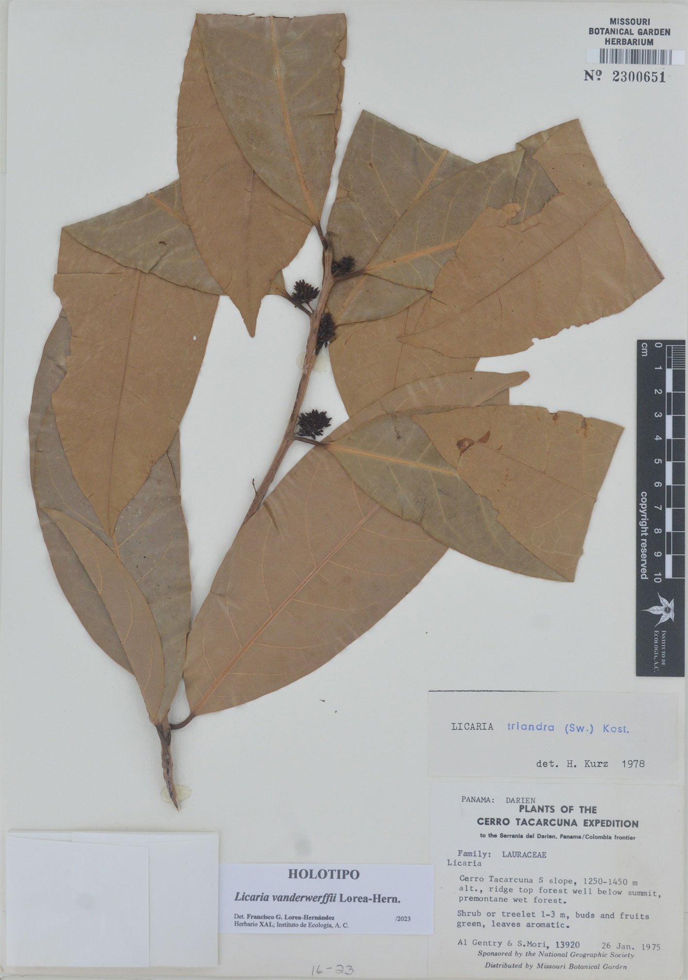
Figure 16. Licaria vanderwerffii Lorea-Hern. sp. nov., general view.
Taxonomic summary
Type. Panama. Darién: Cerro Tacarcuna S slope, 1,250-1,450 m, 26 January 1975, A. Gentry & S. Mori 13920 (holotype MO 2300651; isotype F 1763407).
Etymology. The species is named after Hendrik (Henk) Hessel van der Werff, a prolific scholar of the family Lauraceae in the Neotropics.
Distribution and habitat. So far, only known from the type collection, in the mountains of the southeastern edge of Panama, where premontane rain forest prevails.
Phenology. Flowers in winter; probably ripe fruits expected during autumn or early winter, since maturation of fruits in most Lauraceae takes around a year after flowering.
Conservation status. The place of the type collection is within the boundaries of the nature reserve Parque Nacional del Darién, but the altitudinal range within which the specimen was collected stretches barely for 40 km along the reserve. So, the species should be considered endangered.
Remarks
The collection on which the description of L. vanderwerffii is based was cited by Kurz (2000) as L. triandra, but there are several features that separate the former from this species. Whereas L. triandra presents branchlets solid, paniculate inflorescences (up to 6 cm long), stamens fused throughout (or almost so), glands at the base of filaments, anthers partially exserted, and hypanthium glabrous inside, L. vanderwerffii has hollow branchlets, sub-capitate inflorescences (up to 2 cm long), stamens free, no glands at the base of filaments, anthers wholly exserted, and hypanthium densely white tomentose inside.
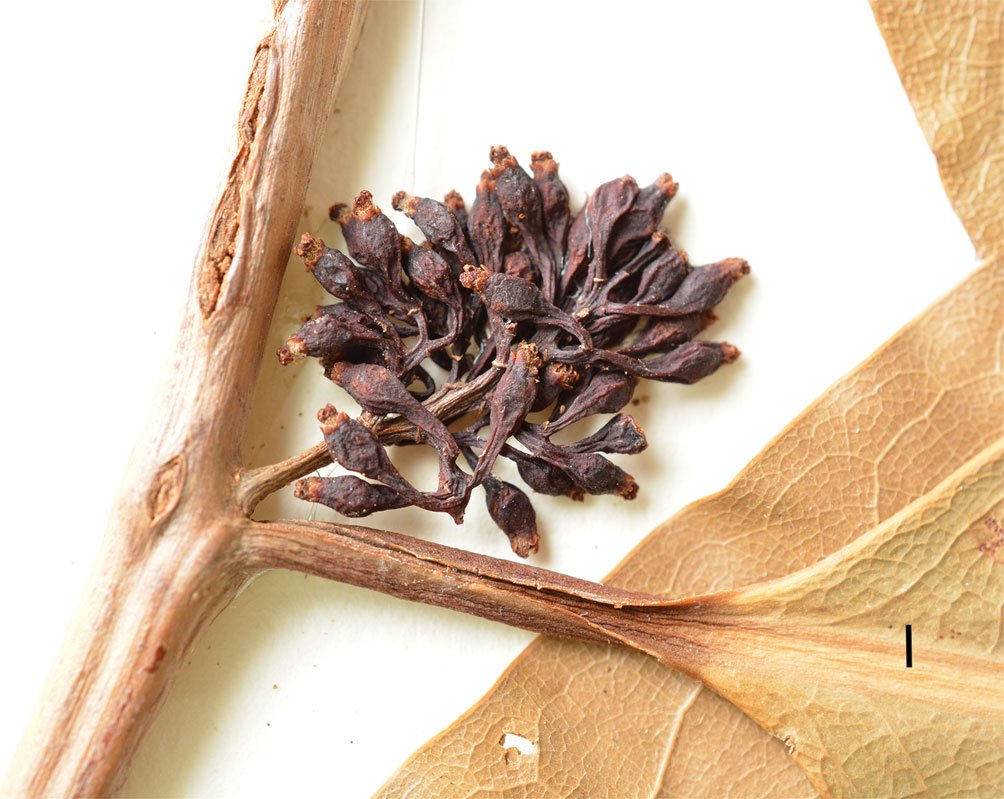
Figure 17. Inflorescence detail of Licaria vanderwerffii Lorea-Hern. sp. nov. Scale bar 1 mm.
This species is closely related to L. agglomerata; both present small, glomerate inflorescences, ellipsoid to narrowly rhomboid flowers with erect tepals, no staminodes, fully exserted stamens, no glands on filaments, pubescent stamens, and hypanthium tomentose within. However, L. vanderwerffii differs by having stamens free throughout, white tomentum on stamens and (densely on) inner face of hypanthium, and glabrous pistil, against stamens fused by their filaments, brownish-orange tomentum on stamens and upper part of hypanthium inside (sometimes completely glabrous), and puberulent style in L. agglomerata. It is worth to mention that they differ in ecological conditions as well; while L. agglomerata grows in lowland habitats (200-700 m), L. vanderwerffii is a mountain dweller above 1,200 m.
Acknowledgements
I would like to thank the curators of the herbaria cited in the Materials and methods section for allowing the study of specimens of Licaria in their collections. I also thank Jens Rohwer and an anonymous reviewer for their comments and calling my attention to several slips and wrong phrasing in some paragraphs. Eva Piedra assisted me with the preparation of figures. Phil Brewster kindly reviewed the final english version of the manuscript. I thank one of the reviewers who suggested to include the following exsiccata as part of the studied material for several of the species described here, however, it was not possible to see the specimens. So even they correspond to duplicates of the studied material, they are cited here just as a reference for researchers who might need to study them.
L. breedlovei; D. Breedlove 50394, isotype TEX 472525.
L. dolichopoda; B. Hammel et al. 16790, isotypes CR 147811 and CR 2918355; E. Bello & E. Cruz 4262, paratype CR 1596155; G. Herrera 4000, paratype CR 1596509; G. Herrera 4510, paratypes CR 159602, CR 176525 and CR 1561583; J. Marín & G. Marín 499, paratype CR 1596363.
L. gibbitepala; G. Herrera & A. Chacón 2427, isotype CR 1596536.
L. minutiflora; G. Herrera 500, isotype CR 151205; E. Bello 784, paratype CR 1513414; E. Bello 2208, paratype CR 1596135; Q. Jiménez & G Rivera 1011, paratypes CR 1561584 and CR 157780; G. Herrera 2942, paratype CR 1596539.
L. tomentulosa; G. Herrera 2165, isotypes CR 146925 and CR 2921047; G. Herrera 2056, paratypes CR 147034, and CR 2920969; G. Herrera 4115, paratypes CR 1596519, and CR 207025; A. Chacón 25, paratype CR 1596195.
References
Burger, W., & van der Werff, H. (1990). Flora Costaricensis. Family 80 Lauraceae. Fieldiana, Botany, n. s., 23, 1–129.
Gómez-Laurito, J., & Cascante, A. (1999). Licaria caribaea (Lauraceae): a new species from the Caribbean lowlands of Costa Rica. Novon, 9, 199–201. https://doi.org/10.2307/3391798
Gómez-Laurito, J., & Estrada, A. (2002). Licaria leonis (Lauraceae), una nueva especie del Pacífico costarricense, y algunas notas sobre Licaria multinervis H. Kurz. Lankesteriana, 3, 5–9. https://doi.org/10.15517/lank.v2i1.23136
Hammel, B. E. (1986). New species and notes on Lauraceae from the Caribbean lowlands of Costa Rica. Journal of
the Arnold Arboretum, 67, 123–136. https://doi.org/10.5962/bhl.part.27389
Kostermans, A. J. G. H. (1937). Revision of the Lauraceae II. The genera Endlicheria, Cryptocarya (American species) and Licaria. Recueil des Travaux Botaniques Néerlandais, 34, 500–609.
Kurz, H. W. (1983). Fortpflanzungsbiologie einiger Gattungen neotropischer Lauraceen und Revision der Gattung Licaria (Lauraceae) (Ph.D. Thesis). University of Hamburg, Germany.
Kurz, H. W. (2000). Revision der Gattung Licaria (Lauraceae). Mitteilungen aus dem Institut für Allgemeine Botanik in Hamburg, 28/29, 89–221.
Mez, C. (1889). Lauraceae americanae. Jahrbuch des Königlichen Botanischen Gartens und des Botanischen Museums zu Berlin, 5, 1–556.
Radford, A. E., Dickison, W. C., Massey, J. R., & Bell, C. R. (1974). Vascular plant systematics. New York: Harper & Row.
Van der Werff, H. (1988). Eight new species and one new combination of Neotropical Lauraceae. Annals of the Missouri Botanical Garden, 75, 402–419. https://doi.org/10.2307/2399431
Van der Werff, H. (2009). Nine new species of Licaria (Lauraceae) from tropical America. Harvard Papers in Botany, 14, 145–159. https://doi.org/10.3100/025.014.0206

Dos especies nuevas neotropicales del género Calymmaderus (Coleoptera: Ptinidae), asociadas con madera estructural en Taretan, Michoacán, México
César Marco Aurelio Jurado-Vargas a, *, José Cruz-de León b, José Tulio Mendez-Montiel c
a Universidad Michoacana de San Nicolás de Hidalgo, Facultad de Biología, Laboratorio de Investigación en Invertebrados, Ciudad Universitaria, Av. Fco. J. Mujica s/n, 58030 Morelia, Michoacán, México
b Universidad Michoacana de San Nicolás de Hidalgo, Facultad de Ingeniería en Tecnología de la Madera, Laboratorio de Conservación y Preservación de la Madera, Ciudad Universitaria, Av. Fco. J. Mujica s/n, 58030 Morelia, Michoacán, México
c Universidad Autónoma Chapingo, Dirección de Ciencias Forestales, Carretera Federal México-Texcoco Km 38.5, 56230 Texcoco, Estado de México, México
*Autor para correspondencia: cjurado@umich.mx (C.M.A. Jurado-Vargas)
Recibido: 02 abril 2024; aceptado: 11 marzo 2025
http://zoobank.org/urn:lsid:zoobank.org:pub:4737516A-ED56-4106-B714-86B23F67BCF4
Resumen
A partir de un análisis morfológico y taxonómico de adultos del género Calymmaderus Solier, 1849 (Ptinidae: Dorcatominae), se describen y proponen 2 nuevas especies para el Neotrópico en México: C. robustus sp. nov. y C. semioblongus sp. nov. Ellas se distinguen de las 7 especies reportadas y reconocidas actualmente para México con base en su coloración, pubescencia y estrías elitrales laterales. Se describe la estructura genital de machos.
Palabras clave: Carcoma; Edificios históricos; Xilófagos
Two new Neotropical species of the genus Calymmaderus (Coleoptera: Ptinidae), associated to structural wood in Taretan, Michoacán, Mexico
Abstract
Through morphological and taxonomic analysis of adults of the genus Calymmaderus Solier, 1849 (Ptinidae: Dorcatominae), 2 new Neotropical species in Mexico are described and proposed: C. robustus sp. nov. and C. semioblongus sp. nov. They are distinguished from the 7 species currently reported and recognized for Mexico based on their coloration, pubescence and lateral elitral striae. The genital structure of males is described.
Keywords: Woodworm; Historic buildings; Xylophages
Introducción
El género Calymmaderus incluye especies de escarabajos xilófagos de distribución mundial, para el cual se reconocen 89 especies americanas (Blackwelder, 1945; Lüer y Honour, 2017; Toskina, 2000; White, 1974, 1982, 1983, 1984), de las que 7 especies se encuentran en México: C. dejeani (Pic, 1905), C. donckieri (Pic, 1904), C. oblongus (Gorham, 1883), C. pupatus (Gorham, 1883), C. semirufus (Champion, 1913), C. sharpi (Gorham, 1886) y C. subvestitus (Champion, 1913) (White, 1983; Zaragoza et al., 2016). El estudio de las especies de este género es complicado debido a la falta de revisiones taxonómicas, lo limitado de sus descripciones diagnósticas y la carencia, en la mayoría de los casos de ilustraciones de los órganos genitales, estudio que le da mayor robustez a la determinación de especies (Bercedo et al., 2008; Lüer y Honour, 2017; Viñolas, 2018). Los miembros de Calymmaderus se distinguen de las demás especies de Ptinidae por su cuerpo alargado y oblongo, antenas con los 2 últimos segmentos de la clava estrechamente unidos, coxas protorácicas expuestas ventralmente, un lóbulo metasternal bifurcado que aloja al último segmento antenal cuando el cuerpo está en reposo y el número de suturas elitrales laterales (Arango, 2012; Español, 1992; White, 1971). Las especies de este género son de importancia económica al dañar la madera estructural de edificios históricos y bienes culturales. La especie más conocida en México es C. oblongus (Gorham, 1883), a la que varios autores señalan como asociada al deterioro de la madera (Bercedo et al., 2008; Cibrián et al., 1995; Jurado-Vargas, 2020; Jurado-Vargas y Cruz, 2010, 2020; Jurado-Vargas et al., 2003; Pichardo et al., 2017; White, 1974).
El presente estudio tiene como objetivo describir 2 especies nuevas de Calymmaderus, que fueron encontradas en la localidad de Taretan, Michoacán, México, ubicada en la Zona de Transición Mexicana, que es un área de alta diversidad y endemismos de artrópodos y presenta la mayor mezcla biótica entre elementos neárticos y neotropicales (Halffter, 2017). Ambas especies representan taxones morfológicamente diferentes a las especies descritas en la literatura conocida para este grupo. White fue el último investigador que publicó datos sobre especies de Calymmaderus y otros géneros de escarabajos de la familia Ptinidae americanas entre 1981 y 1984, dejando pendientes algunos ejemplares con estatus incierto aún por resolver. En este trabajo presentamos la descripción y propuesta de las 2 nuevas especies de Calymmaderus referidas.
Materiales y métodos
El área de estudio corresponde a la localidad de Taretan, Michoacán, México (1,140 m snm, 19°20’3.32” N, 101°55’3.02” O) (fig. 1), que presenta un clima cálido A (w), con precipitación media anual de 1,240 mm y temperatura media anual 25° C (INEGI, 2010).
Se recolectaron 463 ejemplares del género Calymmaderus de la techumbre de madera del templo de San Ildefonso por medio de 2 trampas de luz blanca, durante el periodo de emergencia de los adultos en los meses de junio-agosto del 2017 y 2018. Los ejemplares se fijaron en una solución de alcohol al 80%. La determinación de los ejemplares se realizó usando descripciones y claves de identificación para el género y especies de Calymmaderus (Arango, 2012; White,1971, 1974, 1982, 1983, 1984). En el proceso, la preparación de los órganos se realizó mediante la técnica de montaje permanente en laminillas con resina sintética (Gaviño et al., 2004).
La descripción de los caracteres morfológicos de los ejemplares adultos se realizó mediante un microscopio estereoscópico Nikon a 45 aumentos. Se obtuvieron imágenes de los ejemplares en posición dorsal, lateral y ventral, además de metasterno, abdomen y antenas, mediante un microscopio estereoscópico Carl Zeiss (modelo Axio Zoom V16). Las imágenes de las preparaciones de la estructura genital se lograron a través de un microscopio compuesto Marca Leica a 100 aumentos y una cámara Panasonic adaptada a la distancia focal del ocular. Para obtener detalles adicionales de la morfología externa de los ejemplares, se tomaron imágenes por medio del microscopio electrónico de barrido modelo JSM-6400.
Se determinaron las medidas de largo y ancho de 30 ejemplares de cada una de las especies que se describen con un vernier digital, con las que se realizó un análisis estadístico descriptivo básico de los parámetros utilizados para su descripción. La fenología de emergencia de adultos se determinó mediante gráficos de los registros mensuales de captura de los ejemplares adultos en los periodos de trabajo. Los holotipos y paratipos de las 2 especies se depositaron en la Colección de Invertebrados (Insectos Xilófagos) de la Facultad de Biología de la Universidad Michoacana (CIFBUM-XIL).
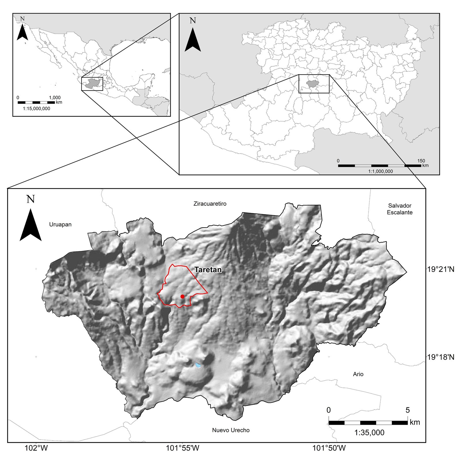
Figura 1. Ubicación de Taretan, localidad tipo de las 2 nuevas especies de Calymmaderus (INEGI, 2016).
Resultados
Descripciones
Calymmaderus robustus Jurado-Vargas sp. nov. (figs. 2-7, 14)
http://zoobank.org/urn:lsid:zoobank.org:act:1C158DC5-F92E-4A6C-A089-09DC362DFC6E
Diagnosis. Cuerpo robusto en vista lateral, 1.9 veces más largo que ancho, color negro uniforme mate, pubescencia blanquecina decumbente y abundante, separada menos de su longitud, élitros paralelos después de la base hasta 3/4 partes; antenas desde la base de café rojizo a café negruzco en los últimos segmentos; metasterno con menos pubescencia que resto del cuerpo. Lóbulo mestasternal con muesca profunda en forma característica de U.
Holotipo ♂, largo 3.8 mm, ancho 2.1 mm. Cuerpo robusto en vista lateral, 1.9 veces más largo que ancho (figs. 2, 3), color negro mate, excepto en palpos maxilares y labiales, que presentan el segmento basal café oscuro y los otros segmentos café rojizo. Tarsos de color café rojizo. Pubescencia decumbente blanquecina, abundante, uniforme en todo el cuerpo. Puntuaciones elitrales de la superficie ampliamente distribuidas, no alineadas e intercaladas con otras puntuaciones diminutas en todo el cuerpo y separadas 1.0 veces su diámetro. Cabeza: ojos grandes y abultados, distancia interocular 1.1 veces el diámetro vertical de un ojo. Clava antenal ligeramente mayor (1.1 veces) que el resto de los segmentos; 9º segmento de la clava antenal ligeramente más largo que los segmentos 10º y 11º (fig. 6). Pronoto: acampanado, 1.9 veces más ancho que largo; borde anterior curvo y márgenes laterales redondeados. Superficie densamente punteada y pilosa, con las puntuaciones laterales equidistantes y separadas en general el equivalente a su diámetro; en el disco las puntuaciones son más separadas (1-2 veces su diámetro). Élitro: puntuaciones del disco y laterales separadas de 1 a 2 veces su diámetro (algunas veces un poco más separadas y alargadas); puntuaciones más cercanas a la base elitral más aglutinadas y puntuaciones laterales hacia la parte distal del élitro más alargadas; ranura lateral visible después de la base del tercer esternito hasta el ápice (fig. 4), abarcando menos de la mitad del élitro. Metasterno: convexo, más ancho que largo, carinas bien delimitadas; puntuaciones cercanas al proceso metasternal más pequeñas, separadas 1.0 veces su diámetro; puntuaciones se agrandan más hacia la parte media y a los lados, separadas de 1.0 a 1.5 veces su diámetro; en la parte media y hasta el borde posterior son más pequeñas y menos densas; surco longitudinal corto y no muy marcado (fig. 5). Abdomen: primero, segundo y quinto esternitos más o menos del mismo largo; segundo con borde posterior ligeramente curvo en centro; tercero un poco más corto que anteriores, y cuarto más corto que el resto (fig. 3). Edeago: longitud: 1.1 mm; anchura 0.48 mm. Parámeros bifurcados apicalmente, con borde apical redondeado; piezas accesorias de los parámeros 4.2 veces más largos que su ancho, con pilosidad larga desde la mitad hasta su extremo. Endófalo: ápice más esbelto que la base, terminando en punta con un diente curvo en forma de gancho, saco interno provisto de por lo menos doce espinas transversales a lo largo; las 2 más cercanas a la base 2 veces más largas que las demás y de posición paralela; 2 espinas al centro más pequeñas y entrecruzadas con las espinas basales más largas (fig. 14).
Paratipo ♀. Aspecto general del cuerpo similar al macho. Largo 4.1 ancho 2.3 mm, ojos evidentemente más grandes y abultados que el macho, distancia interocular 1.3 veces el diámetro vertical de un ojo. Tercera y cuarta sutura de los esternitos curvada a los lados.
Resumen taxonómico
Etimología. El epíteto de la especie robustus deriva de la forma robusta del tórax en vista lateral (mucho más alta que el abdomen), que caracteriza y diferencia a los ejemplares de esta especie en comparación con las especies conocidas.
Material examinado. Holotipo ♂: CIFBUM-XIL Núm. 224. México: Michoacán. Taretan. 19.VII.2017. C. Jurado Col. Trampa de luz blanca, madera estructural de pino. 19°20’3.32” N. 101°55’3.02” O. 1,140 m snm. Paratipos: 28; 13 ♂, 17 ♀. CIFBUM-XIL Núms. 226-252, con los mismos datos del holotipo.
Comentarios taxonómicos
Variabilidad: largo 3.1-4.2 mm (media 3.72) ancho 1.7-2.3 mm (media 2.08). Macho más pequeño que la hembra (de 3.1 a 3.7 mm; tabla 1). Ojos más pequeños, distancia interocular de 1.0 a 1.1 veces del diámetro vertical del ojo; último esternito normal, con sutura recta. Hembra: 3.8 a 4.2 mm, ojos más grandes y abultados que el macho, distancia interocular de 1.2 a 1.3 veces el diámetro vertical de un ojo; último esternito con sutura ligeramente curvada en el centro. Especie con morfología poco variable; color general negruzco mate, pubescencia blanquecina uniforme, algunas veces con pubescencia menos abundante en el metasterno.
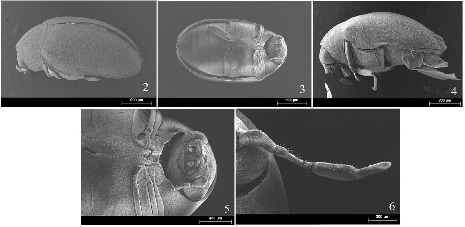
Figuras 2-6. Calymmaderus robustus sp. nov. 2) Vista dorsal; 3) vista ventral; 4) vista lateral; 5) metasterno; 6) antena.
Especie de hábitos nocturnos asociada con madera estructural de Pinus sp.; los ejemplares se capturaron en el interior de la techumbre de madera del templo de “San Ildefonso” Taretan, con trampa de luz. La emergencia de adultos inicia la última semana de junio, con máximo a mediados de julio y disminuye la última semana de julio; la emergencia es rara en agosto. Cohabita con otras especies de Ptinidae y termes, reinfestando durante muchos años la madera del mismo sitio (fig. 7).
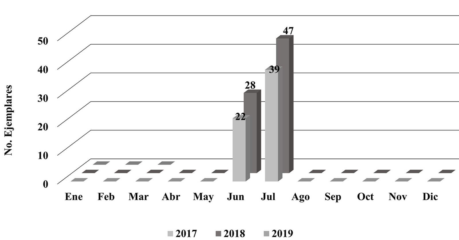
Figura 7. Emergencia adultos de Calymmaderus robustus sp. nov., en 2 ciclos anuales.
Tabla 1
Medidas y variación de largo y ancho de machos y hembras adultos de Calymmaderus robustus sp. nov.
| Medidas | Promedio (mm) | Error estándar | Rango (mm) | |||
| N (hembras) = 13 N (machos) = 17 | Machos | Hembras | Machos | Hembras | Machos | Hembras |
| Longitud | 3.438 | 3.947 | 0.055 | 0.032 | 3.1 – 3.7 | 3.8 – 4.2 |
| Ancho | 1.931 | 2.194 | 0.036 | 0.020 | 1.2 – 2.1 | 2.1 – 2.3 |
De acuerdo con la clave de identificación usada para especies de Calymmaderus (White, 1983), los ejemplares son definitivamente diferentes a las descripciones de las especies mexicanas descritas, considerando la variación en el conjunto de los siguientes caracteres. Todas las especies citadas para México presentan cuerpo oblongo o semiesférico (C. sharpi) en vista lateral; en cuanto al color, los ejemplares descritos de todas las especies van de café rojizo o café oscuro a casi negro, mientras que la coloración del integumento de la especie que se describe es negro mate uniforme. En cuanto a la pubescencia, a diferencia de las especies conocidas en las que tiene tonalidades amarillentas a grisáceas, la especie propuesta presenta pubescencia blanquecina, que contrasta fuertemente con el color del cuerpo. La mayoría de las poblaciones de las especies comparten un tamaño de longitud y ancho similares, excepto C. donckieri y C. subvestitus, que son notablemente más pequeñas. La carencia de información acerca de la armadura genital de las especies no permite hacer comparaciones al respecto. Sin embargo, se presenta la comparación de la armadura genital del macho de las 2 especies propuestas en este documento y C. oblongus, especie mejor conocida de amplia distribución en México (figs. 14-16), lo que respalda la diferenciación entre ellas.
Calymmaderus semioblongus Jurado-Vargas sp. nov. (figs. 8-13, 15)
http://zoobank.org/urn:lsid:zoobank.org:act:7170D451-739D-4507-96C3-A826C5BA4E13
Diagnosis. Forma oblonga, esbelto en vista dorsal, 2.1 veces más largo que ancho, élitros paralelos después de la base hasta 3/4 partes de su extensión; superficie del cuerpo de coloración homogénea de café oscuro a casi negro; pubescencia amarillenta densa y decumbente, separada menos del largo de su longitud; puntuaciones laterales de élitros más agrandadas en la base que en el resto del élitro.
Holotipo ♂, largo 3.8 mm, ancho 1.8 mm. Coloración de café oscuro a casi negro; superficie brillante; antenas y tarsos con la misma coloración del cuerpo; palpos labiales y palpos maxilares café rojizo. Cuerpo oblongo y alargado, 2.1 veces más largo que ancho (figs. 8, 9). Vestidura: pubescencia amarillenta, densa, decumbente y abundante en todo el cuerpo, puntuaciones uniformes en todo el cuerpo, excepto las puntuaciones laterales del élitro que se presentan de forma aglutinada e irregular (fig. 10). Cabeza: ojos pequeños separados 1.4 veces el diámetro vertical de un ojo. Clava antenal 1.3 veces más larga que el resto de los segmentos, noveno segmento de la clava antenal del mismo largo que el décimo y undécimo (fig. 12). Pronoto: acampanado 1.6 veces más largo que ancho, convexo dorsalmente; margen lateralmente redondeado, con un reborde lateral y borde anterior regularmente curvo, no proyectado; disco no prominente; pubescencia uniforme, superficie densamente punteada. Élitro: puntuaciones elitrales irregulares, no alineadas en hileras, separadas de 1 a 2 veces su diámetro, en el disco elitral también a la misma distancia; puntuaciones laterales de la base un poco más grandes y algunas están separadas el equivalente a su diámetro; en el tercio posterior del élitro las puntuaciones son más pequeñas; puntuaciones basales laterales aglutinadas formando una estría a la altura del segundo esternito, que continua hasta el ápice ya bien marcada como ranura basal; por encima otra línea no muy marcada forma otra estría también a nivel del segundo esternito, la ranura ocupa ligeramente más de la mitad del élitro hasta el ápice. Metasterno: ancho del lóbulo metasternal, escasamente mayor que su longitud, muesca profunda, ápice del lóbulo muy arqueado en forma de V; puntuaciones más grandes cerca del lóbulo y a lo largo del borde anterior del metasterno, separadas el equivalente a su diámetro; a los lados las puntuaciones son más espaciadas de 1.0 a 1.5 veces su diámetro, algunas separadas hasta 2 veces su diámetro; del centro hasta el borde posterior, las puntuaciones son más pequeñas y escasas, separadas de 1.0 a 2.0 veces su diámetro; surco longitudinal ligeramente marcado y extendido hasta la mitad del metasterno (fig. 11). Abdomen: segundo ventrito más largo que el resto; el primero y tercero de largo similar, el cuarto es el más estrecho, el quinto presenta una concavidad paralela al ventrito cerca del borde posterior (fig. 9). Edeago: longitud 0.65 mm; anchura 0.41 mm, parámeros bifurcados apicalmente, el más grande de apariencia bilobulada en el extremo; piezas accesorias de los parámeros 4.5 veces más largos que anchos, con pilosidades desde la mitad hasta el ápice. Endofalo: ápice redondeado, saco interno con un par de dientes paralelos al endofalo en la base; sobre estos dientes, hay 2 dientes adicionales curvos con aspecto de media luna (fig. 15).
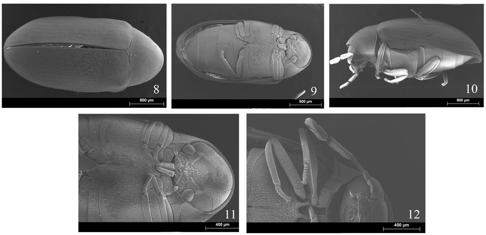
Figuras 8-12. Calymmaderus semioblongus sp. nov. 8) Vista dorsal; 9) vista ventral; 10) vista lateral; 11) metasterno; 12) antena.
Paratipo ♀. Aspecto general del cuerpo similar al macho. Largo 4.1 mm. Ancho 1.9 mm. Distancia interocular 1.4 veces el diámetro vertical del ojo, segunda y tercera suturas abdominales curvadas en el centro, quinta sutura ligeramente curvada a los lados.
Resumen taxonómico
Etimología. El epíteto semioblongus es aplicado por la similitud morfológica externa con la especie oblongus, conocida para varias localidades de México.
Material examinado. Holotipo ♂: CIFBUM-XIL No. 253, Michoacán, Taretan. 18.VIII.2017. C. Jurado Col. Trampa de luz blanca, madera estructural de pino. Col. C. Jurado. 19°20’3.32” N. 101°55’3.02” 0. 1,150 m.snm. Paratipos: 29 individuos CIFBUM-XIL Núms. 255 a 282 (14 ♂ y 14 ♀), mismos datos que el holotipo.
Comentarios taxonómicos
Variabilidad: largo: 3.0-4.8 mm; ancho 1.4- 2.1 mm. Especie muy homogénea. Los machos notablemente menores que las hembras, con tamaño que varía de 3.0 a 3.7 mm (a veces hasta 3.8 mm), con ojos más pequeños y menos separados que en las hembras (distancia interocular de 0.8 a 1.2 el diámetro vertical de un ojo); área frontal algo más aplanada que la hembra, surco longitudinal del metasterno más largo que en la hembra.
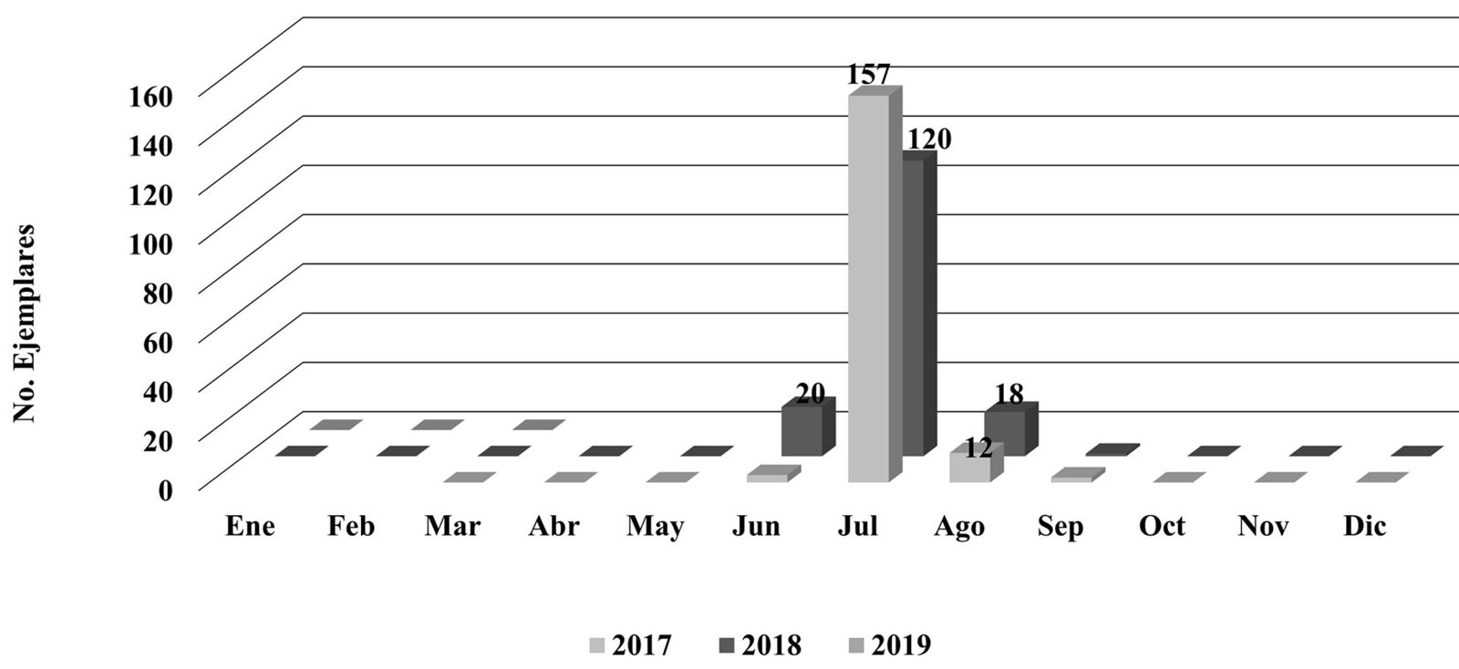
Figura 13. Emergencia de Calymmaderus semioblongus sp. nov., en 2 ciclos anuales.
Tabla 2
Medidas y variación de largo y ancho de machos y hembras adultos de Calymmaderus semioblongus sp. nov.
| Medidas | Promedio (mm) | Error estándar | Rango (mm) | |||
| N (machos) = 15 N (hembras) = 15 | Machos | Hembras | Machos | Hembras | Machos | Hembras |
| Longitud | 3.507 | 4.133 | 0.059 | 0.070 | 3.0-3.8 | 3.8-4.8 |
| Ancho | 1.627 | 1.886 | 0.025 | 0.026 | 1.4-1.7 | 1.7-2.1 |
Tabla 3. Medidas y variación de largo y ancho de machos y hembras adultos de Calymmaderus oblongus de la localidad de Tacícuaro, Michoacán.
| Medidas | Medidas | Promedio (mm) | Error estándar | Rango (mm) | |||
| N (machos) = 15 N (hembras) = 15 | n♂= 15 n♀= 15 | ♂ | ♀ | ♂ | ♀ | ♂ | ♀ |
| Longitud | Longitud | 3.507 | 4.133 | 0.060 | 0.070 | 3.0-3.8 | 3.8-4.8 |
| Ancho | Ancho | 1.627 | 1.887 | 0.025 | 0.026 | 1.4-1.7 | 1.7-2.1 |
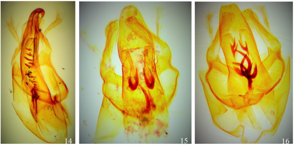
Figura 14-16. Estructura genital de machos de las 3 especies de Calymmaderus vistas al microscopio compuesto 100X: 14) C. robustus sp. nov; 15) C. semioblongus sp. nov; 16) C. oblongus.
Hembra: cuerpo más grande que el macho, de 3.9 a 4.8 mm, ojos más grandes y separados que el macho (distancia interocular de 1.4 a 1.6 veces el diámetro vertical del ojo), última sutura esternal más curva a los lados que en el macho.
Especie de hábitos nocturnos asociada con madera estructural de Pinus sp. Se capturó en el interior de la techumbre de madera del templo de San Ildefonso en Taretan, Michoacán, con trampa de luz. La emergencia de los adultos inicia la última semana del mes de junio, en el mes de julio se registra la máxima emergencia con el inicio del verano, hasta disminuir en agosto con pocos ejemplares y en septiembre su emergencia es rara. Cohabita con otras especies xilófagas de Ptinidae y de termitas. Reinfesta las estructuras de madera por muchos años en el mismo sitio (fig. 13).
Calymmaderus semioblongus sp. nov. es una especie diferente a las otras especies mexicanas del género (White, 1983). Muestra similitud morfológica con la especie oblongus, pero con diferencias evidentes como la coloración del integumento (café oscuro en la especie descrita, a diferencia de oblongus que tiende más a café rojizo; sus medidas de longitud y ancho del cuerpo son menores (3.0 a 4.5 mm de longitud y ancho 1.4 a 2.1 mm, tabla 2), en comparación con C. oblongus (de 3.3 a 5.2 mm de largo y ancho de 1.6 a 2.4 mm, tabla 3). Ambas especies presentan de 2 a 3 hileras de puntuaciones laterales desde la base elitral que forman estrías; en oblongus, la estría más externa y cercana a la ranura elitral es más corta y las otras 2 estrías son menos marcadas que en la especie que se describe. La comparación de la estructura genital de machos de C. oblongus y C. semioblongus sp. nov. también mostró diferencias claras en el número y posición de espinas en el endofalo de estas 2 especies; C. oblongus presenta 2 espinas en forma de cornamenta en la parte más alejada de la base (figs. 14-16).
Agradecimientos
Al Laboratorio de Investigación en Invertebrados de la Facultad de Biología y a la División de Estudios de Posgrado de la Facultad de Ingeniería en Tecnología de la Madera de la UMSNH, por apoyar el proyecto de insectos xilófagos en madera estructural en Michoacán. A Mauricio Quesada, jefe del laboratorio Nacional de Síntesis Ecológica, ENES, UNAM, Unidad Morelia, por facilitar el uso del microscopio Axiostar Zoom V16, para la toma de imágenes de ejemplares. A las autoridades eclesiásticas del Templo de la “Asunción” de Taretan (en especial al párroco Francisco Javier Valencia Durón), por permitir el trabajo de campo en el inmueble. A Roberto Sibaja por la elaboración y ubicación del mapa del sitio. Finalmente agradecer a José Fernando Villaseñor Gómez, de la Facultad de Biología, quien colaboró en la última revisión del texto, con sugerencias acertadas y positivas.
Referencias
Arango, R. A. y Young, D. K. (2012). Death-watch and spider beetles of Wisconsin—Coleoptera: Ptinidae. USDA Forest Service, Forest Products Laboratory, General Technical Report FPL-GTR-209. https://doi.org/10.2737/FPL-GTR-209
Bercedo, P., García, B. R. y Arnaiz, L. (2008). El género Calymmaderus Solier, 1849 nuevo para Canarias y descripción de una nueva especie (Coleoptera: Ptinidae: Dorcatominae). Boletín de la Sociedad Entomológica Aragonesa, 42, 33–35.
Blackwelder, R. E. (1945). Checklist of the coleopterous insects of México, Central America, The West Indies, and South America (Ptinidae, Gnostidae and Anobiidae). Bulletin of the United States National Museum, 185, 401–406. https://doi.org/10.5479/si.03629236.185.3
Cibrián, T. D., Méndez M. J. T., Campos, B. R., Harry, O. Y. y Flores, L. J. (1995). Insectos forestales de México. Texcoco, Estado de México: Universidad Autónoma Chapingo.
Español, C. F. (1992). Coleoptera: Anobiidae. Fauna Ibérica, Vol. 2. Museo Nacional de Ciencias Naturales. Madrid: CSIC.
Gaviño, G., Juárez, L. C. y Figueroa, T. H. (2004). Técnicas biológicas selectas de laboratorio y campo. México D.F.: Limusa.
Halffter, G. (2017). La Zona de Transición Mexicana y la megadiversidad de México: del marco histórico a la riqueza actual. Dugesiana, 2, 77–89. https://doi.org/10.32870/dugesiana.v24i2.6572
INEGI (Instituto Nacional de Geografía y Estadística). (2010). Compendio de información geográfica municipal. Taretan, Michoacán de Ocampo. Clave geoestadística 16087. Instituto Nacional de Geografía y Estadística. Recuperado el 17 diciembre, 2024 de: https://www.inegi.org.mx/contenidos/app/mexicocifras/datos_geograficos/16/16087.pdf
Jurado-Vargas, C. M. A. (2020). Incidencia y daño de insectos en la techumbre de madera de cinco edificios históricos (Templos) de Michoacán (Tesis doctoral). Facultad de Ingeniería en Tecnología de la madera, Universidad Michoacana de San Nicolás de Hidalgo. Morelia, Michoacán.
Jurado-Vargas, C. M. A., Campos, B. R. y Cruz-de León, J. (2003). Anóbidos asociados a la madera en uso en dos monumentos históricos de Michoacán. Entomología Mexicana, 2, 803–806.
Jurado-Vargas, C. M. A. y Cruz-de León, J. (2010). Insectos que dañan la madera de edificios históricos de Morelia, Michoacán. Entomología Mexicana, 9, 103–110.
Jurado-Vargas, C. M. A. y Cruz-de León, J. (2020). Evaluación de la incidencia de insectos xilófagos en la madera estructural del Templo de Ucareo en Michoacán. Entomología Mexicana, 7, 389–395.
Lüher, A. H. y Honour, R. (2017). Descripción de dos especies nuevas de Calymmaderus Solier, 1849 (Coleoptera: Ptinidae) de Chile. Boletín de la Sociedad Entomológica Aragonesa, 60, 105–110.
Pichardo, S. L., San Marino, C. A., Jiménez, Q. E. y Torres, H. B. (2017). Familia Ptinidae. En D. Cibrian-Tovar (Ed.), Fundamentos de entomología forestal (pp. 268–272). Texcoco, Estado de México: Universidad Autónoma Chapingo.
Toskina, I. N. (2000). New wood-boring beetles (Coleoptera: Anobiidae) from Paraguay. Russian Entomological Journal, 9, 199–240.
Viñolas, A. (2018). Nuevos datos sobre la validez específica de Ernobius vinolasi Novoa y Baselga, 2000 (Coleoptera: Ptinidae: Ernobiinae). Arquivos Entomoloxicos, 19, 75–80. https://doi.org/10.5281/zenodo.12767756
White, R. E. (1971). Key to North American genera of Anobiidae, with phylogenetic and synonymic notes (Coleoptera). Annals of the Entomological Society of America, 64, 179–191. https://doi.org/10.1093/aesa/64.1.179
White, R. E. (1974). The Dorcatominae and Tricoryninae of Chile (Coleoptera: Anobiidae). Transactions of the American Entomological Society, 100, 191–253.
White, R. E. (1982). A catalog of the Coleoptera of America North of Mexico. Family Anobiidae. Systematic Entomology Laboratory, Agricultural Research Service, U.S. Dept. of Agriculture, U.S.A.
White, R. E. (1983). Keys to Neotropical species of Calymmaderus Solier and species of Calytheca White, taxonomic notes (Coleoptera: Anobiidae). Proceedings of the Entomological Society of Washington, 85, 229–250.
White, R. E. (1984). Eight new species of Anobiidae (Coleoptera) from Jamaica. The Coleopterists Bulletin, 38, 240–248.
Zaragoza, S., Navarrete-Heredia, J. L. y Ramírez, G. E. (2016). Temolines. Los coleópteros entre los antiguos mexicanos. Ciudad de México: Instituto de Biología, UNAM. Disponible: http://www.ibiologia.unam.mx/barra/publicaciones/Temolines.pdf

Eukaryotic diversity and trophic levels inside the tank bromeliad Pseudalcantarea grandis in a dry area as detected by eDNA metabarcoding
José Alan Herrera-García a, Mahinda Martinez a, b, *, Pilar Zamora-Tavares c, Ofelia Vargas c, Luis Hernández-Sandoval a, b
a Universidad Autónoma de Querétaro, Facultad de Ciencias Naturales, Av. de las Ciencias, s/n, 76230 Juriquilla, Querétaro, Mexico
b Universidad Autónoma de Querétaro, Facultad de Ciencias Naturales, Biología, Laboratorio Nacional de Identificación y Caracterización Vegetal, Av. de las Ciencias, s/n, 76230 Juriquilla, Querétaro, Mexico
c Universidad de Guadalajara, Centro Universitario de Ciencias Biológicas y Agropecuarias, Instituto de Botánica, Departamento de Botánica y Zoología, Laboratorio Nacional de Identificación y Caracterización Vegetal, Av. Ing. Ramón Padilla Sánchez, 45200 Zapopan, Jalisco, Mexico
*Corresponding author: mahinda@uaq.mx (M. Martínez)
Received: 20 May 2024; accepted: 19 February 2025
Abstract
Some bromeliads form a compact rosette that accumulates detritus and water, known as phytotelma. The phytotelma is a lentic ephemeral aquatic environment that forms diverse communities with complex trophic levels. Pseudalcantarea grandis, a saxicolous plant, forms a phytotelma. To understand the importance of P. grandis as a eukaryotic diversity reservoir in arid zones, we collected water samples from 5 plants growing in a dry canyon in Zimapán, Hidalgo, Mexico. We analyzed them through metabarcoding of the ITS1 (Internal Transcribed Spacer) and the partial 5.8S gene. We used the Ion Torrent PGM platform for the sequencing, and the taxonomic assignation for the amplicons was made with BLAST in Genbank at NCBI. We found 26 phyla and 543 genera, 80% of which belonged to Ascomycota, Basidiomycota, Blastocladiomycota Chytridiomycota, Glomeromycota, Mucoromycota, and Zoopagomycota phyla. The remaining 20% was composed of 19 phyla belonging to other kingdoms. Photosynthetic organisms were represented by the phyla Bacillariophyta, Charophyta, Chlorophyta, and Ochrophyta. The vascular plants do not live in the tank but constitute the debris sustaining the large number of decomposers. The trophic levels in the tank were detritus, micro- and macro-decomposers, filter feeders, photosynthesizers, micro-predators, aquatic volume predators, surface predators, and parasites.
Keywords: Aquatic; Ephemeral; Arid zone; Phytotelma
Diversidad de eucariotes y niveles tróficos dentro de la bromelia tanque Pseudalcantarea grandis en una zona árida detectados por metabarcoding de ADN ambiental
Resumen
Algunas bromelias forman rosetas compactas que acumulan detritus y agua. Esta acumulación se conoce como fitotelma, un hábitat acuático léntico y efímero con comunidades diversas y niveles tróficos complejos. Psedalcantarea grandis es una planta saxícola y forma un fitotelma. Para entender la importancia de P. grandis como reservorio de diversidad acuática en una zona árida, colectamos muestras de agua de 5 plantas en un cañón de Zimapán, Hidalgo, México y las analizamos por metabarcoding del ITS1 (Internal Transcribed Spacer) y una región parcial del gen 5.8S. La secuenciación se hizo en la plataforma Ion Torrent PGM. Asignamos la identidad taxonómica de los amplicones utilizando BLAST de Genbank. Encontramos 26 phyla y 543 géneros, 80% pertenecen a los phyla fúngicos Ascomycota, Basidiomycota, Blastocladiomycota Chytridiomycota, Glomeromycota, Mucoromycota, y Zoopagomycota. El 20% restante está compuesto por 19 phyla de otros reinos. Los organismos fotosintéticos estuvieron representados por los phyla Bacillariophyta, Charophyta, Chlorophyta y Ochrophyta. Otros organismos fotosintéticos que corresponden a plantas vasculares no viven dentro del tanque, pero forman la hojarasca que mantiene a los descomponedores. Los niveles tróficos en el tanque fueron detritus, micro y macrodescomponedores, filtradores, fotosintetizadores, microdepredadores, depredadores del volumen de agua, depredadores de superficie y parásitos.
Palabras clave: Acuático; Efímero; Zona árida; Fitotelma
Introduction
The Bromeliaceae family is comprised of almost 3,700 species distributed mostly in tropical areas of the Americas (Gouda et al., 2024). They are herbaceous perennial monocots with leaves arranged in rosettes, many of which are epiphytes (Ramírez-Murillo et al., 2004; Rzedowski, 2006). There are 442 species in Mexico (Espejo-Serna & López-Ferrari, 2018) that frequently grow in nutrient and mineral-deficient environments (Bernal et al., 2006; Ramírez-Murillo et al., 2004). Some species form compact rosettes with absorbent trichomes in their interior that allow the accumulation of solids rich in nutrients and water, known as phytotelma (Benzing, 2000; Goffredi et al., 2011).
Phytotelmata are lentic aquatic environments, mostly ephemeral that last less than 3 months (Mogi, 2004). They are freshwater habitats for diverse communities including viruses, Archaea, and bacteria (Brouard et al., 2013, Goffredi et al., 2011). Among the eukaryotes, aquatic mosses, green algae, diatoms, protists, fungi, insects, amphibians, and crustaceans have been documented (Benzing, 2000; Brandt et al., 2017; Kitching, 2001; Ramos & do Nascimento Moura, 2019; Rodríguez-Núñez et al., 2018; Simão et al., 2020).
Bromeliads that form phytotelma accumulate essential mineral elements, which are the main nitrogen source for the plant (Kitching, 2001). The presence of detritivores and predators is related to the nitrogen concentration in the leaves. Predators increase nutrient flux from the leaf litter of nearby plants to the bromeliad (Benzing & Renfrow, 1974; Ngai & Srivastava, 2006; Nievola et al., 2001; Takahashi & Mercier, 2011).
Unlike terrestrial and aquatic communities in which plants and algae are the main nutrient resources, in the phytotelma leaf litter and invertebrate remains play that role. In trophic networks inside the phytotelma, protists and rotifers are considered as micro-predators that also consume organic particles. Macroinvertebrates can consume the detritus, filter feeders, aquatic predators, and surface predators, whereas bacteria and fungi are the main decomposers that obtain energy directly from the detritus (Brouard et al., 2012; Mogi, 2004).
Gomes et al. (2015) characterized the enzymatic activity of the fungal community inside the bromeliad tank of Vriesea minarum in Brazil. Using cultivation techniques they identified 36 species, 22 of which were Basidiomycota and 14 were Ascomycota. The most relevant genera were Cryptococcus, Candida, and Aureobasidium. These organisms contain enzymes that degrade vegetal material.
Nutrient intake for the plant is further facilitated by insects (Ngai & Srivastava, 2006). For example, odonatan larvae ingest detritivores, contributing to the nitrogen cycle within the bromeliad by defecating. Leachates from defecation release nitrogen in a form available to the bromeliad and create a suitable niche for other microorganisms providing substrata (Benzing & Renfrow, 1974).
Pseudalcantarea grandis (Schltdl.) Pinzón & Barfuss (Fig. 1A) is a saxicolous tank bromeliad that reaches 2.5 m in height and forms a highly ramified inflorescence in March and April. It is distributed from Central Mexico (Guanajuato, Querétaro, Hidalgo) toward the south (Puebla, Oaxaca, and Chiapas) and into Honduras. It is considered a MegaMexico II endemic species (Espejo-Serna et al., 2010). At the locality of Las Adjuntas, in Hidalgo, the plant is known as “tinaja”, “jarilla”, and “soluche de agua” because its tank can store water. The species grows in crags of the main rivers in the northeastern portion of the region known as Bajío. It grows at elevations ranging from 400 to 1,600 m asl (Espejo-Serna et al., 2010; Rzedowski, 2006).
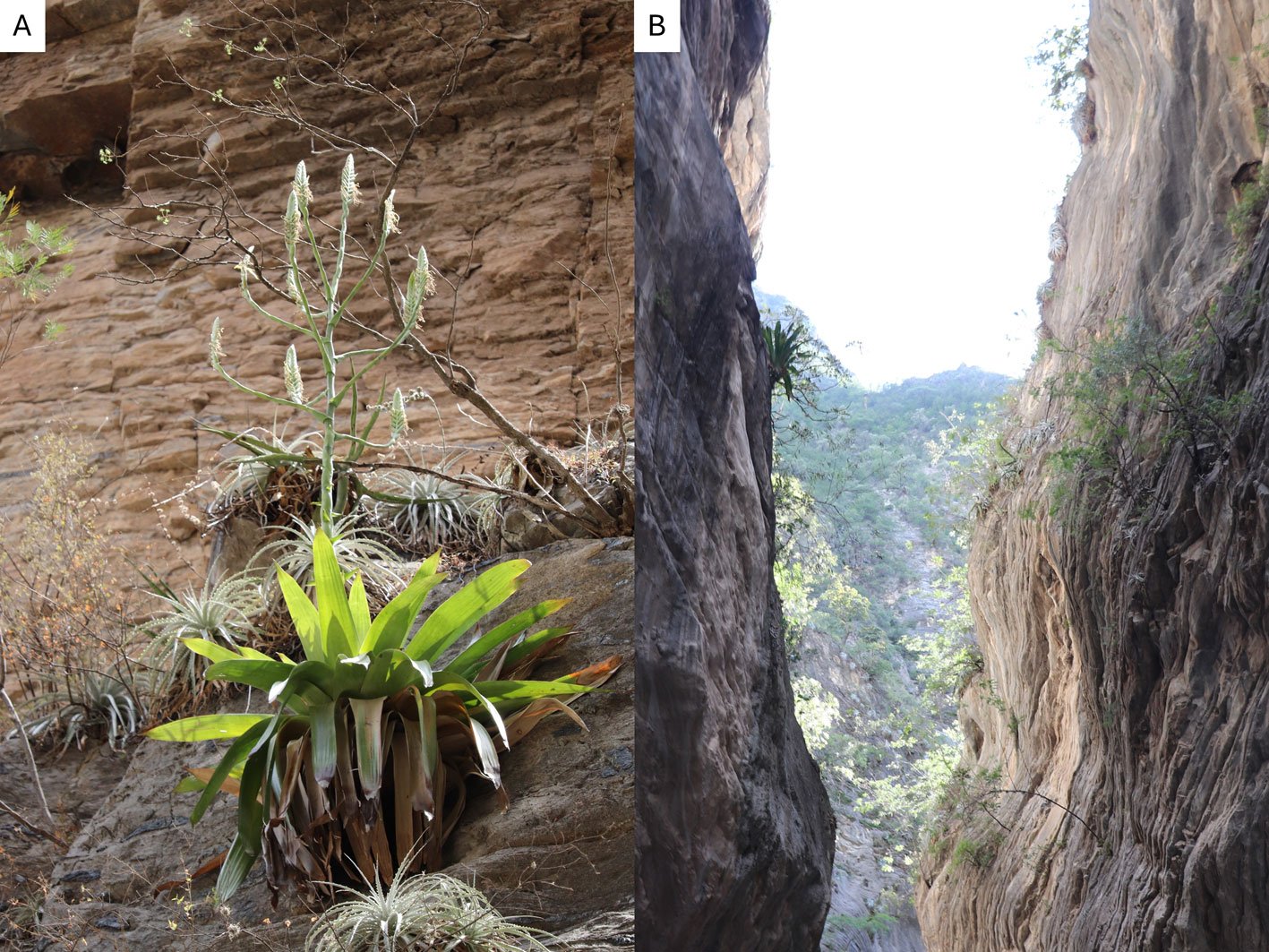
Figure 1. Life form and habitat of the tank bromeliad Pseudalcantarea grandis. A, Plant and inflorescence of Pseudalcantarea grandis; B, Las Angosturas Canyon crags where the tank bromeliad grows.
Metabarcoding studies describing the communities associated with phytotelma have mostly focused on specific groups such as vertebrates (Brozio et al., 2017), ciliates (Simão et al., 2017), or bacteria (Louca et al., 2017; Rodríguez-Núñez et al., 2018). In Pseudalcantarea grandis, 297 bacteria genera were found, with Proteobacteria (37%), Actinobacteria (19%), and Firmicutes (15%) comprising the highest percentage (71%). The main metabolic functions were aerobic chemoheterotrophy and fermentation. However, rare biosphere bacteria were also found, which could favor micro-ecosystem resilience and resistance (Herrera-García et al., 2022). Comprehensive sequencing of the eukaryotic diversity inside tank bromeliads has been performed in tropical zones (Simão et al., 2020), but not arid areas. The objectives of our study were to describe the eukaryotic diversity in Pseudalcantarea grandis phytotelma to understand which vascular plants form the litter, and to infer the putative trophic levels of the phytotelmata in an arid zone.
Materials and methods
Water samples were collected during the 2018 rainy season at Las Angosturas Canyon, Zimapán, Hidalgo, Mexico (20°50.933’ N, 99°26.7’ W, 900 m asl, see Herrera-García et al. [2022] for a location map) within the Queretano-Hidalguense arid zone, which has been described as a high-diversity and endemicity area (Hernández-Magaña et al., 2017; Hernández & Bárcenas, 1995; Rojas et al., 2013). This arid zone is considered the southernmost portion of the Chihuahuan Desert floristic province. It consists mostly of arid valleys and depressions surrounded by mountains (Hernández & Gómez-Hinostrosa, 2005).
Las Angosturas Canyon is approximately 12 km long with a mixture of xerophytic scrub and tropical deciduous forest (Fig. 1B). Bromeliads grow on vertical crags with different amounts of the surrounding vegetation. Therefore, the tanks are frequently filled with leaf litter. We selected individuals that were accessible enough to be collected by a rappel and were more than 50 cm in diameter. The associated plants are listed in Table 1. To collect the water inside the bromeliads we used Nest® cell scrapers to scratch the inside of each tank, and the water in the bromeliads was vigorously shaken to obtain a homogeneous sample. Water volumes of 50 to 100 ml were collected using 10 ml sterile serological pipettes. The samples were stored in 50 ml conical Falcon tubes, transported on dry ice, and stored at -79 °C until processing. Physicochemical water parameters were not determined.
Table 1
Las Angosturas Canyon floristic inventory. Plants directly above the sampled individuals are noted in the second column. Vouchers and photographs are noted in the third column.
| Family | Species | Association | Reference at QMEX |
| Amaryllidaceae | Zephyranthes clintiae Traub | A. Herrera 30 | |
| Amaryllidaceae | Zephyranthes concolor (Lindley) Bentham & Hook. | A. Herrera 7 | |
| Anacardiaceae | Rhus terebinthifolia Schltdl. & Cham. | A. Herrera 21 | |
| Anacardiaceae | Pseudosmodingium virletii (Baill.) Engl. | L. Hernández 5029 | |
| Apocynaceaea | Asclepias curassavica L. | A. Herrera 20 | |
| Apocynaceaea | Vallesia glabra (Cav.) Link | A. Herrera 4 | |
| Arecaceae | Brahea dulcis (Kunth) Mart. | Photographic record | |
| Asparagaceae | Agave xylonacantha Salm-Dyck | surrounding | A. Vega 50 |
| Asparagaceae | Dasylirion longissimum Lem. | L. Hernández 4511 | |
| Asparagaceae | Yucca filifera Chab. | L. Hernández 4828 | |
| Asparagaceae | Yucca queretaroensis Piña | Photographic record | |
| Asteraceae | Baccharis salicifolia (Ruiz y Pav.) Pers. | M. Martínez 6056 | |
| Asteraceae | Cirsium sp. | A. Herrera ND | |
| Asteraceae | Gnaphalium luteo-album L. | A. Herrera ND | |
| Asteraceae | Gochnatia hypoleuca (DC.) A. Gray | surrounding | A. Herrera ND |
| Bignoniaceae | Tecoma stans (L.) Juss. | Photographic record | |
| Boraginaceae | Cordia boissieri A. DC. | M. Martínez 7144 | |
| Bromeliaceae | Hechtia glomerata Zucc. | surrounding | S. Zamudio 14469 |
| Bromeliaceae | Hechtia tillandsioides (André) L. B. Smith | surrounding | Photographic record |
| Table 1. Continued | |||
| Family | Species | Association | Reference at QMEX |
| Bromeliaceae | Pseudalcantarea grandis (Schltdl.)Pinzón & Barfuss | A. Herrera 1 | |
| Bromeliaceae | Tillandsia recurvata L. | surrounding | M. Martínez 8220 |
| Burseraceae | Bursera morelensis Ram. | surrounding | Photographic record |
| Cactaceae | Astrophytum ornatum (DC.) Britton & Rose | Photographic record | |
| Cactaceae | Cylindropuntia imbricata (Haw.) F. M. Knuth ssp. cardenche (Griffiths) U. Guzmán | A. Herrera 12 | |
| Cactaceae | Coryphanta sp. | Photographic record | |
| Cactaceae | Echinocereus pentalophus Lem. | Photographic record | |
| Cactaceae | Echinocactus platyacanthus Link & Otto | M. Figueroa 12 | |
| Cactaceae | Ferocacutus histrix (DC.) G.E.Linds. | Photographic record | |
| Cactaceae | Mammilaria elongata DC. | surrounding | Photographic record |
| Cactaceae | Mammillaria longimamma DC. | Photographic record | |
| Cactaceae | Myrtillocactus geometrizans (Mart. ex Pfeiff.) Console | surrounding | Photographic record |
| Cactaceae | Neobuxbaumia polylopha (DC.) Backeberg | Photographic record | |
| Cactaceae | Opuntia imbricata (Haw.) F. M. Kunth | Photographic record | |
| Cactaceae | Opuntia microdasys (Lehm.) Pfeiff. | Photographic record | |
| Cactaceae | Opuntia rastrera F.A.C. Weber | surrounding | Photographic record |
| Cactaceae | Stenocereus queretaroensis (F.A.C.Weber ex Mathes.) Buxb. | Photographic record | |
| Cactaceae | Strombocactus disciformis (DC.) Britton & Rose | Photographic record | |
| Cannabaceae | Celtis pallida Torr. | A. Herrera 2 | |
| Capparaceae | Capparis incana Kunth | A. Herrera 5 | |
| Convolvulaceae | Ipomoea rzedowskii E. Carranza | A. Herrera 17 | |
| Crassulaceae | Echeveria secunda Booth | surrounding | A. Herrera 26 |
| Crassulaceae | Pachyphytum sp. | A. Herrera ND | |
| Crassulaceae | Sedum sp. | surrounding | A. Herrera ND |
| Euphorbiaceae | Cnidoscolus tubulosus (Muell. Arg.) I.M. Johnst. | A. Herrera 9 | |
| Euphorbiaceae | Acalypha monostachya Cav. | A. Herrera 15 | |
| Euphorbiaceae | Croton ciliato-glandulifer Ort. | L. Hernández 5029 | |
| Euphorbiaceae | Jatropha dioica Sessé ex Cerv. | A. Herrera ND | |
| Euphorbiaceae | Ricinus communis L. | A. Herrera ND | |
| Fabaceae | Acacia berlandieri Benth. | surrounding | Photographic record |
| Fabaceae | Albizia occidentalis Brandegee | Photographic record | |
| Fabaceae | Bauhinia sp. | Photographic record | |
| Fabaceae | Lysiloma microphylla Bentham | A. Herrera 36 | |
| Fabaceae | Mimosa leucaenoides Bentham | surrounding | Photographic record |
| Fabaceae | Mimosa martindelcampoi F. G. Medrano | Photographic record | |
| Fabaceae | Mimosa puberula Bentham | A. Herrera 3 | |
| Fabaceae | Pithecellobium dulce (Roxb.) Bentham | Photographic record | |
| Fabaceae | Neltuma laevigata (Humb. & Bonpl. ex Willd.) Britton & Rose | M. Martínez ND | |
| Fabaceae | Vachellia farnesiana (L.) Willd. & Arn. | A. Herrera 10 | |
| Table 1. Continued | |||
| Family | Species | Association | Reference at QMEX |
| Fouquieriaceae | Fouquieria splendens Engelm. | surrounding | Photographic record |
| Lentibulariaceae | Pinguicula aff. moctezumae Zamudio & R.Z. Ortega | Photographic record | |
| Lythraceae | Heimia salicifolia (Kunth) Link | A. Herrera 13 | |
| Onagraceae | Hauya elegans DC. | surrounding | A. Herrera 14 |
| Malpighiaceae | Mascagnia macroptera (Moc. & Sessé ex DC.) Nied. | A. Herrera 8 | |
| Malvaceae | Pseudobombax ellipticum (Kunth) Dugand | A. Herrera ND | |
| Malvaceae | Malvaviscus arboreus Cav. | M. Martínez 5317 | |
| Myrtaceae | Psidium guajava L. | surrounding | Photographic record |
| Papaveraceae | Argemone ochroleuca Sweet | M. Martínez 6713 | |
| Plantaginaceae | Rusellia polyedra Zucc. | A. Herrera 27 | |
| Platanaceae | Platanus mexicana Moric. | A. Herrera 16 | |
| Poaceae | Arundinaria sp. | A. Herrera ND | |
| Poaceae | Cenchrus sp. | A. Herrera ND | |
| Poaceae | Cynodon dactylon (L.) Pers. | M. Martínez 3197 | |
| Poaceae | Eragrostis sp. | E. Carranza 5251 | |
| Primulaceae | Samolus ebracteatus Kunth | A. Herrera 11 | |
| Pteridaceae | Argyrochosma formosa (Liebm.) Windham | A. Herrera 23 | |
| Pteridaceae | Notholaena affinis (Mett.) T. Moore | A. Herrera 24 | |
| Pteridaceae | Notholaena jacalensis Pray | A. Herrera 25 | |
| Pteridaceae | Pellaea sp. | A. Herrera 34 | |
| Ranunculaceae | Clematis drummondii Torr. & A.Gray | M. Martínez 4434 | |
| Rhamnaceae | Karwinskia subcordata Schlecht. | A. Herrera 22 | |
| Rubiaceae | Nernstia mexicana (Zucc. & Mart. ex DC.) Urb. | A. Herrera 32 | |
| Salicaceae | Neopringlea integrifolia (Hemsl.) S. Watson | A. Herrera 19 | |
| Salicaceae | Salix humboldtiana Willd. | Photographic record | |
| Sapindaceae | Dodonaea viscosa (L.) Jacq. | A. Herrera ND | |
| Sapindaceae | Sapindus saponaria L. | A. Herrera ND | |
| Sapindaceae | Serjania sp. | A. Herrera ND | |
| Selaginellaceae | Selaginella lepidophylla (Hook. & Grev.) Spring. | surrounding | Photographic record |
| Selaginellaceae | Selaginella ribae Valdespino | A. Herrera 29 | |
| Selaginellaceae | Selaginella selowii Hieron. | A. Herrera 28 | |
| Solanaceae | Datura inoxia Miller | V. Martínez 1 | |
| Solanaceae | Nicotiana glauca Graham | Photographic record | |
| Solanaceae | Nicotiana trigonophylla Dunal | O. García 434 | |
| Solanaceae | Physalis cinerascens (Dunal) Hitch. | L. Hernández 3769 | |
| Solanaceae | Physalis philadelphica Lam. | A. Herrera 38 | |
| Solanaceae | Solanum lycopersicon L. | Photographic record | |
| Taxodiaceae | Taxodium mucronatum Ten. | M. Martínez 3237 | |
| Urticaceae | Urera sp. | H. Rubio 302 | |
| Zygophyllaceae | Morkillia acuminata Rose & Painter | surrounding | A. Herrera 18 |
DNA extraction
Water samples were homogenized and 100 ml was filtered through a 0.22 µm Millipore® nitrocellulose membrane. The membrane was frozen and macerated in liquid nitrogen. We extracted total DNA using the QIAmp DNA Extraction® kit following the manufacturer’s instructions by duplicate to obtain pseudoreplicates and verify reproducibility. DNA quality and concentration were evaluated using NanoDrop® spectrophotometry.
Amplicon sequencing
To characterize eukaryotic diversity, we amplified a portion of the 5.8 S Internal Transcibed Spacer (ITS) with the ITS1 and ITS2 primers designated by White et al. (1990). The PCR reaction consisted of a final volume of 25 µl, that contained 2 mM of dNTP´s, 2mM µl of each primer, 0.4% DMSO, 0.4 % BSA, 2.5 mM MgCl2, 1.2 mM Buffer, 1.25 U Platinum Taq, 60ng/µl DNA and H2O. Thermocycler conditions were an initial step at 95 °C for 3 min, followed by 30 cycles at 95 °C for 1 min; 52 °C, 45 s, and 72 °C, 2 min, with a final extension step at 72 °C for 5 min. Amplicons were purified with Agencourt® AMPure® XP.
To construct the libraries, we used the Ion Plus Fragment Library kit. The presence, size, and concentration of the fragment were analyzed using Bioanalyzer 2100 with high-sensitivity DNA assay (Agilent). Libraries were quantified using real-time PCR to obtain an equimolar dilution factor to mix the 3 libraries. The template was prepared using a PCR emulsion in the Ion One Touch 2 System (Life Technologies) and quantified by fluorometry in Qubit® 3.0 (Thermo Fisher Scientific). Finally, the template was loaded onto the PGM 318TM chip using the 400-pair base fragment sequencing kit, according to the Ion PGM™ Hi‑Q™ View Sequencing Kit protocol.
We sampled the vascular plants growing at the canyon, directly above the bromeliad, and also the surrounding vegetation. Voucher specimens were deposited at QMEX herbarium. We compared the similarity of the plant inventory obtained by sequencing against the floristic list obtained by field sampling through a Sorensen coefficient analysis at the family level.
Sequencing quality was evaluated using the FastQC program. Sequences were filtered by the quality value of Phred > 20. We selected sequences larger than 100 bp in the CLC Genomic Workbench v.11.01 (QIAGEN Bioinformatics, Aarhus, Denmark) platform. In the Microbial Genomics module application, we performed an analysis based on the amplicons to aggregate the sequences in operational taxonomic units (OTUs) considering only 99% similarity among them. We deleted unique reads and chimeras. Taxonomic assignation of the amplicons was performed with BLAST in 2023 via the Genbank at NCBI database (Altschul et al., 1990). Over 90% of the OTUs had identity percentages higher than 95% and only 54 OTUs had lower percentages, ranging from 75 to 80%. We manually reviewed them and corroborated the genus of each one. Since BLAST provides determinations at the genus and species levels, we used MEGAN Community Edition V. 6.24.4 to assign kingdom, phylum, class, order, and family. We loaded the BLAST results using the lowest basal common ancestor assignation algorithm (LCA). The analysis is based on the taxonomic hierarchies recognized by NCBI and the results are displayed as a phylogenetic tree that allows simple observation of taxonomic diversity (Huson et al., 2016). We manually reviewed the classifications and to corroborate the taxonomic assignations we used the classification proposed by Simpson (2006) for plants, and Tree of Life (2022) for the other eukaryotic marine taxa (such as Cnidaria). The OTUs at the genus level were used to define the total eukaryotic group diversity present in our sample.
We assigned the ecological function of each genus following the criteria of Mogi (2004) and Brouard et al. (2012). We considered 9 categories: 1) detritus formed by leaf litter and vegetal matter that serves as the main resource for the trophic network; 2) micro decomposers integrated by bacteria (Herrera-García et al., 2022); 3) macro decomposers formed by saprobiotic fungi; 4) filter feeders that use small particles including microorganisms that are in turn consumed by aquatic and surface predators; 5) photosynthetic organisms that require sunlight and serve as food for predators; 6) micro predators that feed on photosynthetic organisms, filter feeders, and micro-decomposers; 7) aquatic predators which are macroinvertebrates that live in the water column and feed mostly on algae and bacteria; 8) surface predators which are restricted to the uppermost portion of the water column and feed on protists, bacteria, and algae; and 9) parasites which are obligate vertebrate parasites that use arthropods as vectors.
Results
The 5 sampled plants had volumes that varied from 50 to 100 ml. The 2 pseudoreplicates were compared and considered as a single pool due to the similarity of the resulting OTUs. We obtained a total of 3,276,538 lectures. After quality and size filtration, the number of useful lectures was reduced to 1,284,998 representing a total of 23,948 OTUs, 762 of which could not be assigned to the species or genus taxonomic category provided by BLAST.
The diversity of organisms living in the tank consisted of 26 phyla and 543 genera. See Supplementary material T1 for a list of assigned taxa. Fungi were dominant, as 80% of the genera belonged to Ascomycota, Basidiomycota, Blastocladiomycota Chytridiomycota, Glomeromycota, Mucoromycota, and Zoopagomycota phyla. The remaining 20% was composed of 19 phyla: Apicomplexa, Apusozoa, Arthropoda, Bacillariophyta, Bryophyta, Cercozoa, Charophyta, Chlorophyta, Ciliophora, Cnidaria, Colponemidia, Heterolobosea, Hyphochytriomycota, Metamonada, Myxomycota, Ochrophyta, Oomycota, Platyhelminthes, and Tracheophyta (Fig. 2). We identified 25 genera of photosynthetic algae from the phyla Bacillariophyta (with the genera Pseudo-nitzschia, Navicula, and Stephanodiscus), Charophyta (Staurastrum), Chlorophyta (Leskea, Didymogenes, Meyerella, Dolichomastix, Bathycoccus, Mychonastes, Trebouxia, Chamaetrichon, Hazenia, Chloroidium, and Pleurastrum), and Ochrophyta (Nannochloropsis). The other photosynthetic organisms were Bryophyta (Fontinalis, Leskea, and Thuidium).
Protists were represented by 44 genera, 4 of which are relevant to human health: Plasmodium (Apicomplexa) which causes paludism, Giardia (Metamonada) which is responsible for giardiasis, Neobalantidium (Cilliophora) that causes balantidiosis, and Spirometra (Plathelmyntes) which is responsible for sparganosis.
Tracheophyta (vascular plants) do not live in the phytotelma but do constitute the debris that accumulates in the bromeliad. They comprised 11% of the identified genera. We found a Sorensen coefficient of 45% similarity among the methods in which 14 taxa at the family level were shared (Supplementary material F1). Arthropoda were represented by 13 genera of the Coleoptera, Diptera, Hymenoptera, Lepidoptera, Odonata, and Pocopodia orders.
Of the eukaryotic organisms, 79% were classified as decomposers, and 7% were classified as micro-predators. In the tank, 3% were photosynthetic organisms, 2% were parasites, and the remaining 9% corresponded to the vascular plants that constitute the detritus. Tracheophyta and Bryophyta constituted the vegetal resources available to micro- and macro-decomposers, and filter feeders. Cercozoa, Apusozoa, Heterolobosea, and Colponemidia were considered micro-predators because they consume some photosynthetic organisms, filter feeders, and micro-decomposers. Ciliophora and 2 Arthropoda genera (Cyprideis and Notodromas) were some of the filter feeders. Apicomplexa, Chytridiomycota, Metamonada, Myxomycota, and Zoopagomycota were the parasites. Aquatic predators were mostly metazoans (Cnidaria and Platyhelminthes) that use filter feeders, photosynthesizers, and macro decomposers as resources. The arthropods Coleoptera, Diptera, Hymenoptera, Lepidoptera, and Odonata were part of the uppermost categories of the trophic network (surface predators). However, their exoskeletons and/or excretions become part of the tank resource or contribute to the nutrient cycling of the microecosystem (Figs. 3, 4).
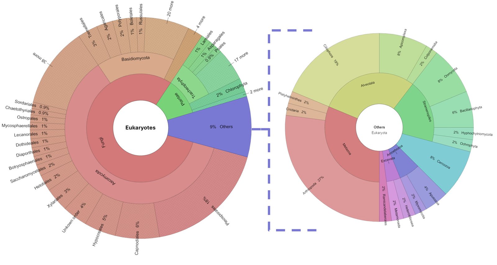
Figure 2. Percentage of eukaryotic diversity present in the Pseudalcantarea grandis tank.
Discussion
Eukaryotic composition of the Pseudalcantarea grandis community
The abundance of fungi in the Pseudalcantarea tank appeared to correlate with their function in the trophic network. Fungi are the most important degrading group, responsible for organic decomposition and nutrient recycling in forests, aquatic ecosystems, and the phytotelma (Costa & Gusmão, 2015; Grossart et al., 2019; Grothjan et al., 2019). Fungi also have multiple functions in aquatic environment interactions that favor antagonistic and symbiotic members of the community. They can be predators, parasites, or food for heterotrophic protists. Some can use organic matter, pollen, or zooplankton exoskeletons (Zoopagomycota, Chytridiomycota) (Grossart et al., 2019). Vegetal matter decomposition enhances detritus quality for detritivores degrading vegetal polysaccharides into monosaccharides through enzymatic reactions which are then easily digested by microorganisms (Krauss et al., 2011). Fungi and protist interactions for vegetal matter transformation are poorly documented. A symbiotic relationship between them is unknown and difficult to study because of the microscopic scale at which they occur (Grossart et al., 2019).
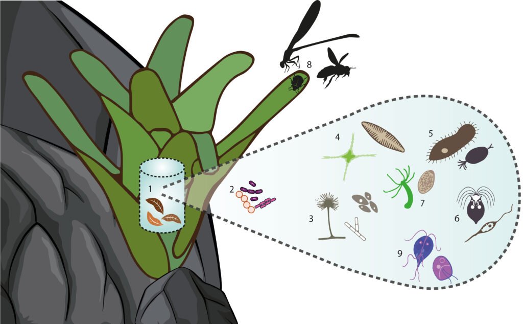
Figure 3. Graphic representation of Pseudalcantarea grandis tank trophic categories. 1 = Detritus, 2 = micro-decomposers, 3 = macro-decomposers, 4 = photosynthesizers, 5 = filter feeders, 6 = micro-predators, 7 = aquatic predators, 8 = surface predators, and 9 = parasites
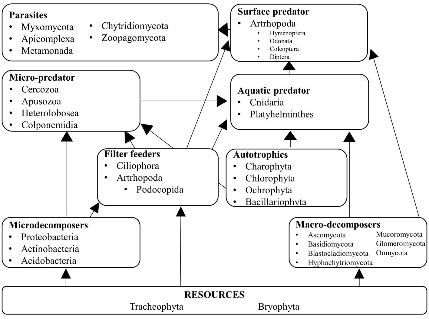
Figure 4. Hypothetical trophic level network inside Pseudalcantarea grandis tank. Examples of taxa are listed.
The fungal diversity found in the Pseudalcantarea grandis tank was high compared to that reported in previous studies of other Bromeliaceae species. We found 436 genera, whereas Gomes et al. (2015) identified 36 genera using cultivation techniques. Other papers already pointed out that metagenomic studies detect higher diversity levels than other techniques (Simão et al., 2020). The 36 genera found by Gomes et al. (2015) were also found in P. grandis. Cryptococcus, Candida, and Aureobasidium have specific enzymatic activity in plant material degradation, which suggests that degradation reactions by these organisms are frequent in the phytotelma. The primers used in our study were developed for fungi (White et al., 1990), therefore they might be overrepresented.
We found 44 protist genera in the phytotelma. Some have mixotrophic nutrition, in that they obtain their energy through photo- and heterotrophy depending on the environmental conditions in which they grow (Jones, 2000). In aquatic environments where light is available but dissolved organic carbon (DOC) is scarce, photosynthetic organisms are better represented. Low light and high DOC favor heterotrophic organisms (Jones, 2000). The latter condition is what was present in the sampled tanks. Therefore, the development of photosynthetic protists is not favored because of the large and abundant bacterial community that competes for elements such as phosphorus (Brouard et al., 2012; Herrera-García et al., 2022). In the rainy season, the tank of P. grandis is surrounded by vegetation that intercepts light and deposits leaf litter, therefore favoring the conditions for fungi and decomposers (Grossart et al., 2019; Herrera-García et al., 2022, Kitching, 2000).
Direct observations and sampling of the phytotelma of tropical zones have revealed Diptera, Odonata, Oligochaeta, Ostracoda, beetles, copepods, pseudoscorpions, scorpions, isopods, Lepidoptera, hemipterans, homopterans, orthopterans, and arachnids in tank bromeliads (Cutz-Pool et al., 2016; Marino et al., 2013). Using environmental DNA with specific primers, amphibians (Brozio et al., 2017) and ciliates (Simão et al., 2017) have been found in tank bromeliads with high water availability. These results suggest that aridity and strong water seasonality in our study area were responsible for the lack of amphibians and the low arthropod and ciliate diversity we found.
Phytotelma seasonality is an important factor. In a rainy forest, the annual precipitation is 3,000 mm and rain is present for 280 days, therefore the water in the tank lasts longer (Brouard et al., 2012). In contrast, in our location, the annual precipitation is 391 mm and the phytotelma is available only through the rainy season from May to June (INFAED, 2012). The presence of Plasmodium is relevant since its most common vector is Aedes, suggesting that at some point during the phytotelma duration, the mosquito is in contact with the water, completing the parasite life cycle (Williams, 2007).
The absence of vertebrates is characteristic of phytotelma communities (Mogi, 2004). One exception is in rainforest bromeliad, where bromeliad tadpoles can be found. We did not find vertebrates. Strong seasonality was probably the reason for their absence. Not all OTUs could be assigned to the species or genus taxonomic category at 99% identity level we used. We did not find an identity for 762 of the 23,984 sequences, possibly because the sequences of these organisms are not available in the NCBI database, or because the organisms have not yet been described.
The tracheophytes found in the phytotelma could not be identified at the generic level. There are 2 possible explanations: the reads were short (150 bp) and therefore insufficient, or the genera growing at the canyon are not in the GenBank NCBI (National Center for Biotechnology Information) database. However, 30 families of vascular plants were detected, 16 of which correspond to the families found by field collection.
Trophic structure of the Pseudalcantarea grandis tank
We propose 9 trophic levels for tank bromeliads in arid zones, —2 more than those suggested by Mogi (2004), and 3 more than those suggested by Brouard et al. (2012). Detritus is the main nutrient source. Macrodecomposers process leaf litter into small organic matter particles, including their waste. The particles are then stored in the phytotelma where filterers and invertebrates process them. Dead organisms, feces, and leaf litter stored at the bottom of the tank are used by bacteria and other microorganisms such as fungi to assimilate nutrients (Brouard et al., 2012). We found that 48 plant genera (45 Tracheophyta, and 3 Bryophyta) constitute the detritus, and although Brouard et al. (2012) recognized organic litter as a resource, they did not identify the organisms that provided it. The large amount of detritus was due to the type of surrounding vegetation, which was a tropical deciduous forest in this study. In P. grandis macro decomposers are fungi of the Ascomycota, Basidiomycota, and Myxomycota phyla. We concur with Brouard et al. (2012) that ciliates are filterers. Mogi (2004) did not consider microorganisms to be autotrophs, but Brouard et al. (2012) included that category, and in P. grandis algae constitute this level. Insects were categorized as surface predators in their diagram; they include the odonate family Coenagrionidae, which includes the 2 genera we found in P. grandis, Ischnura, and Agriocnemis (Brouard et al., 2012). Neither Mogi (2004) nor Brouard et al. (2012) included parasites at a trophic level, but some of the genera found in P. grandis are obligate parasites, mostly from the Alveolata kingdom, which has birds and mammals as hosts but uses arthropods as vectors.
We found 26 phyla with 543 genera in the phytotelma of P. grandis growing in an arid zone. The identified diversity suggested that the organisms that inhabit these small ephemeral water bodies are adapted to prolonged dry spells and develop quickly when the phytotelma has water. The biota was mostly composed of fungi (over 80% of the diversity) that specialize in plant detritus degradation. Water bodies shelter aquatic groups that cannot exist in areas outside the P. grandis phytotelma. It is easier to assess the diversity of organisms within a tank than to comprehend their interactions. The trophic network proposed for eukaryotes indicates that they fulfill different functions.
As final considerations, we conclude that the analyzed phytotelma had a large detritus accumulation, and water was present briefly. Most of the diversity belonged to fungi (80%) because of the large amount of plant detritus in the tank. Photosynthesizers were scarce but included 25 algal genera and 3 Bryophyta. We found 45% Sorensen coefficient similarity between the plant detritus and the specimens collected with herbarium specimens. We also found a low arthropod and ciliate diversity, and the tank also harbors protist genera, some of which have medical implications. We found 9 trophic levels in the tank. Unlike tropical areas, in which algal production can support non-detrital food webs, in our arid zone system, detritus degradation was the main energy source.
Acknowledgments
Funding was provided by Conahcyt through grant 293833 for the Laboratorio Nacional de Identificación y Caracterización Vegetal. Diana Velázquez designed and executed Figure 3. Two anonymous reviewers helped to improve the manuscript with their comments.
References
Altschul, S. F., Gish, W., Miller, W., Myers, E. W., & Lipman, D. J. (1990). Basic local alignment search tool. Journal of Molecular Biology, 215, 403–410. https://doi.org/10.1016/S0022-2836(05)80360-2
Benzing, D. H., & Renfrow, A. (1974). The mineral nutrition of Bromeliaceae. Botanical Gazette, 135, 281–288. https://doi.org/10.1086/336762
Benzing, D. H. (2000). Bromeliaceae: profile of an adaptive radiation. Cambridge, U.K.: Cambridge University Press.
Bernal, R., Valverde, T., & Hernández-Rosas, L. (2006). Habitat preference of the epiphyte Tillandsia recurvata (Bromeliaceae) in a semi-desert environment in Central Mexico. Canadian Journal of Botany, 83, 1238–1247. https://doi.org/10.1139/b05-076
Brandt, F. B., Martinson, G. O., & Conrad, R. (2017). Bromeliad tanks are unique habitats for microbial communities involved in methane turnover. Plant and Soil, 410, 167–179. https://doi.org/10.1007/s11104-016-2988-9
Brouard, O., Céréghino, R., Corbara, B., Leroy, C., Pelozuelo, L., Dejean, A. et al. (2012). Understorey environments influence functional diversity in tank-bromeliad ecosystems. Freshwater Biology, 57, 815–823. https://doi.org/10.1111/j.1365-2427.2012.02749.x
Brozio, S., Manson, C., Gourevitch, E., Burns, T. J., Greener, M. S., Downie, J. R. et al. (2017). Development and application of an eDNA method to detect the critically endangered Trinidad golden tree frog (Phytotriades auratus) in bromeliad phytotelmata. Plos One, 12, 1–8. https://doi.org/10.1371/journal.pone.0170619
Costa, L. A., & Gusmão, L. F. P. (2015). Characterization saprobic fungi on leaf litter of two species of trees in the Atlantic Forest, Brazil. Brazilian Journal of Microbiology, 46, 1027–1035. https://doi.org/10.1590/S1517-838246420140548
Cutz-Pool, L. Q., Ramírez-Vázquez, U. Y, Castro-Pérez, J. M, Puc-Paz, W. A., & Ortiz-León, H. J. (2016). La artropo-
dofauna asociada a Tillandsia fasciculata en bajos inundados de tres sitios de Quintana Roo, México. Entomología Mexicana, 3, 576–581.
Espejo-Serna, A., & López-Ferrari, A. R. (2018). La familia Bromeliaceae en México. Botanical Sciences, 96, 533–554. https://doi.org/10.17129/botsci.1918
Espejo-Serna, A., López-Ferrari, A., & Ramírez-Murillo, I. (2010). Bromeliaceae. Flora del Bajío y Regiones Adyacentes, 165, 1–82.
Goffredi, S. K., Kantor, A. H., & Woodside, W. T. (2011). Aquatic Microbial Habitats Within a Neotropical Rain-
forest: Bromeliads and pH-Associated Trends in Bacterial Diversity and Composition. Microbial Ecology, 61, 529–542. https://doi.org/10.1007/s00248-010-9781-8
Gomes, F. C. O., Safar, S. V. B., Marques, A. R., Medeiros, A. O., Santos, A. R. O., Carvalho, C. et al. (2015). The diversity and extracellular enzymatic activities of yeasts isolated from water tanks of Vriesea minarum, an endangered bromeliad species in Brazil, and the description of Occultifur brasiliensis f.a., sp. nov. Antonie van Leeuwenhoek, International Journal of General and Molecular Microbiology, 107, 597–611. https://doi.org/10.1007/s10482-014-0356-4
Gouda, E. J., Butcher, D., & Dijkgraaf, L. (2024) Encyclopaedia of Bromeliads, Version 5. Utrecht University Botanic Gardens, online (accessed: 02-10-2024): http://bromeliad.nl/encyclopedia/
Grossart, H. P., Van den Wyngaert, S., Kagami, M., Wurzbacher, C., Cunliffe, M., & Rojas-Jimenez, K. (2019). Fungi in aquatic ecosystems. Nature Reviews Microbiology, 17, 339–354. https://doi.org/10.1038/s41579-019-0175-8
Grothjan, J. J., & Young, E. B. (2019). Diverse microbial communities hosted by the model carnivorous pitcher plant Sarracenia purpurea: Analysis of both bacterial and eukaryotic composition across distinct host plant populations. PeerJ, 2019, e6392. https://doi.org/10.7717/peerj.6392
Hernández, H. M., & Bárcenas, R. T. (1995). Endangered Cacti in the Chihuahuan Desert: I. Distribution Patterns. Conservation Biology, 9, 1176–1188. https://doi.org/10.1046/j.1523-1739.1995.9051169.x-i1
Hernández, H. M., & Gómez-Hinostrosa, C. (2005). Cactus diversity and endemism in the Chihuahuan Desert Region. EnJ. L. Cartron, G. Ceballos, & R. Felger (Eds.), Biodiversity, ecosystems and conservation in Northern Mexico (pp264–275). New York: Oxford University Press.
Hernández-Magaña, R., Hernández-Oria, J. G., & Chávez, R. (2017). Datos para la conservación florística en función de la amplitud geográfica de las especies en el Semidesierto Queretano, México. Acta Botanica Mexicana, 140, 105. https://doi.org/10.21829/abm99.2012.22
Herrera-García, J. A., Martínez, M., Zamora-Tavares, P., Vargas-Ponce, O., Hernández-Sandoval, L., & Rodríguez-Zaragoza, F. A. (2022). Metabarcoding of the phytotelmata of Pseudalcantarea grandis (Bromeliaceae) from an arid zone. PeerJ, 10, e12706. https://doi.org/10.7717/peerj.12706
Huson, D. H., Beier, S., Flade, I., Górska, A., El-Hadidi, M., Mitra, S. et al. (2016). MEGAN Community Edition – Interactive Exploration and Analysis of Large-Scale Microbiome Sequencing Data. Plos Computational Biology, 12, 1–12. https://doi.org/10.1371/journal.pcbi.1004957
INAFED (Instituto Nacional para el Federalismo y el Desarrollo Municipal). (2012). Zimapán. Enciclopedia de los municipios y Delegaciones de México. http://www.inafed.gob.mx/work/enciclopedia/EMM13hidalgo/municipios/13084a.html
Jones, R. I. (2000). Mixotrophy in planktonic protists: an overview. Freshwater Biology, 45, 219–226. https://doi.org/10.1046/j.1365-2427.2000.00672.x
Kitching, R. (2000). Food webs and container habitats: the natural history and ecology of phytotelma. Cambridge, U.K.: Cambridge University Press. https://doi.org/10.1017/CBO9780511542107
Kitching, R. L. (2001). Food webs in phytotelmata: “Bottom-Up” and “Top- Down’” Explanations for Community Structure. Annual Review of Entomology, 46, 729–760. https://doi.org/10.1146/annurev.ento.51.110104.151120
Krauss, G. J., Solé, M., Krauss, G., Schlosser, D., Wesenberg, D., & Bärlocher, F. (2011). Fungi in freshwaters: Ecology, physiology and biochemical potential. FEMS Microbiology Reviews, 35, 620–651. https://doi.org/10.1111/j.1574-6976.20
11.00266.x
Louca, S., Jacques, S. M. S., Pires, A. P. F., Leal, J. S., González, A. L., Doebeli, M. et al. (2017). Functional structure of the bromeliad tank microbiome is strongly shaped by local geochemical conditions. Environmental Microbiology, 19, 3132–3151. https://doi.org/10.1111/1462-2920.13788
Marino, N. A. C., Srivastava, D. S., & Farjalla, V. F. (2013). Aquatic macroinvertebrate community composition in tank-bromeliads is determined by bromeliad species and its constrained characteristics. Insect Conservation and Diversity, 6, 372–380. https://doi.org/10.1111/j.1752-4598.2012.00224.x
Mogi, M. (2004). Phytotelmata: hidden freshwater habitats supporting unique faunas. In C. M. Yule, & H. S. Yong (Eds.), Freshwater invertebrates of the Malaysian region (pp. 13–22). Kuala Lumpur, Malaysia: Academy of Sciences Malaysia.
Ngai, J. T., & Srivastava, D. S. (2006). Predators accelerate nutrient cycling in a bromeliad ecosystem. Science, 314, 963. https://doi.org/10.1126/science.1132598
Nievola, C. C., Mercier, H., & Majerowicz, N. (2001). Levels of Nitrogen assimilation in bromeliads. Journal of Plant Nutrition, 24, 1387–1398. https://doi.org/10.1081/PLN-100106989
Ramírez-Murillo, I., Carnevali-Fernández, G., & Chi-May, F. (2004). Guía ilustrada de las Bromeliaceae de la porción mexicana de la península de Yucatán. Yucatán: Centro de Investigación Científica de Yucatán.
Ramos, G. J. P., & do Nascimento Moura, C. W. (2019). Algae and cyanobacteria in phytotelmata: diversity, ecological aspects, and conservation. Biodiversity and Conservation, 28, 1667–1697. https://doi.org/10.1007/s10531-019-01771-2
Rodríguez-Núñez, K. M., Rullan-Cardec, J. M., & Ríos-Velázquez, C. (2018). The metagenome of bromeliads phytotelma in Puerto Rico. Data in Brief, 16, 19–22. https://doi.org/10.1016/j.dib.2017.10.065
Rojas, S., Castillejos-Cruz, C., & Solano, E. (2013). Florística y relaciones fitogeográficas del matorral xerófilo en el valle de Tecozautla, Hidalgo, México. Botanical Sciences, 91, 273–294. https://doi.org/10.17129/botsci.8
Rzedowski, J. (2006). Vegetación de México. México D.F.: Conabio.
Simão, T. L. L., Borges, A. G., Gano, K. A., Davis-Richardson, A. G., Brown, C. T., Fagen, J. R. et al. (2017). Characterization of ciliate diversity in bromeliad tank waters from the Brazilian Atlantic Forest. European Journal of Protistology, 61, 359–365. https://doi.org/10.1016/j.ejop.2017.05.005
Simão, T. L. L., Utz, L. R. P., Dias, R., Giongo, A., Triplett, E. W., & Eizirik, E. (2020). Remarkably complex microbial community composition in bromeliad tank waters revealed by eDNA metabarcoding. Journal of Eucaryotic Microbiology, 67, 593–607. https://doi.org/10.1111/jeu.12814
Simpson, M. G. (2006). Plant systematics. Amsterdam: Elsevier/Academic Press.
Takahashi, C. A., & Mercier, H. (2011). Nitrogen metabolism in leaves of a tank epiphytic bromeliad: characterization of a spatial and functional division. Journal of Plant Physiology, 168, 1208–1216. https://doi.org/10.1016/j.jplph.2011.01.008
Tree of Life Web Project, (2019). Tree of life. Website. http://tolweb.org/tree/
White, T. J., Bruns, T., Lee, S., & Taylor, J. (1990). Amplification and direct sequencing of fungal ribosomal RNA genes for Phylogenetics. In M. A. Innis, D. H. Gelfand, J. J. Sninsky, T. J. White (Eds.), PCR Protocols (January) (pp. 315–322). San Diego, CA: Academic Press. https://doi.org/10.1016/b978-0-12-372180-8.50042-1
Williams, D. D. (2007). Other temporary water habitats. The Biology of temporary waters. Oxford, UK: Oxford University Press. https://doi.org/10.1093/acprof:oso/9780198528128.001.0001

Sea slugs (Gastropoda: Heterobranchia) from Huatulco: new records and distribution range extensions for Oaxaca, Mexico
Oscar Iván González-Romero a, Xochitl G. Vital a, b, *
a Universidad Nacional Autónoma de México, Facultad de Ciencias, Circuito Exterior s/n, Ciudad Universitaria, Coyoacán, 04510 Ciudad de México, México
b Universidad Nacional Autónoma de México, Posgrado en Ciencias Biológicas, Facultad de Ciencias, Circuito Exterior s/n, Ciudad Universitaria, Coyoacán, 04510 Ciudad de México, México
*Corresponding autor: vital@ciencias.unam.mx (X.G. Vital)
Received: 18 August 2024; accepted: 5 February 2025
Abstract
While the diversity of sea slugs in the northern area of the Pacific coast of Mexico has been studied thoroughly in the last decades, little is known about the composition of species in the southern states of Mexico. Several field trips were made in 5 localities of Bahías de Huatulco, Oaxaca, where specialized sampling methods focused on sea slugs were carried out. Herein, we documented 49 species of sea slugs, including 37 new records for the state, which increases to 58 species the total sea slug richness known for Oaxaca. This study updates the inventory of sea slugs for the Mexican Pacific coast and contributes to the knowledge of the marine fauna of the Natural Protected Area “Parque Nacional Huatulco”.
Keywords: Bahías de Huatulco; Coral reefs; Molluscs; Nudibranchia; Tropical Eastern Pacific
Babosas marinas (Gastropoda: Heterobranchia) de Huatulco: nuevos registros y ampliaciones de distribución para Oaxaca, México
Resumen
Mientras que la diversidad de babosas marinas en la zona norte de la costa del Pacífico mexicano ha sido estudiada de forma exhaustiva en las últimas décadas, poco se sabe acerca de la composición de especies en los estados del sur de México. Se realizaron diversas visitas a 5 localidades de las bahías de Huatulco, Oaxaca, donde se llevaron a cabo métodos de muestreo especializados con enfoque en babosas marinas. Aquí censamos 49 especies de babosas marinas, con 37 nuevos registros para el estado, lo que incrementa la riqueza de babosas marinas conocida para Oaxaca a 58 especies. Este estudio actualiza el inventario de babosas marinas para la costa del Pacífico mexicano y contribuye al conocimiento de la fauna marina del Área Natural Protegida “Parque Nacional Huatulco”.
Palabras clave: Bahías de Huatulco; Arrecifes de coral; Moluscos; Nudibranchia; Pacífico este tropical
Introduction
Heterobranch sea slugs are gastropods with more than 8,400 described species distributed in all the oceans of the planet, from the intertidal zone to deep waters (Behrens et al., 2022; Camacho-García et al., 2005). Some of these molluscs can do some of the most exceptional processes in the metazoans, such as the incorporation of functional chloroplasts or nematocysts into their tissues (Goodheart & Bely, 2017; Händeler et al., 2009). Furthermore, sea slugs can be important model organisms in several study areas from neuroscience to global climate change (Kandel, 1979; Ziegler et al., 2014); a source of biomedical compounds used for creating novel drugs (Dean & Prinsep, 2017; Fisch et al., 2017) and an attractive target to professional and amateur underwater photographers worldwide (Behrens, 2005).
More than 370 species of sea slugs have been recorded in the Eastern Pacific from Alaska to Central America (Behrens et al., 2022), of which around 234 have been found on the Mexican Pacific coast (Hermosillo et al., 2006). Although several studies on sea slugs have been performed in this region (e.g., Angulo-Campillo, 2005; Bertsch, 2014; Flores-Rodríguez et al., 2017; Hermosillo, 2009, 2011; Hermosillo & Behrens, 2005; Hermosillo & Gosliner, 2008; Verdín-Padilla et al., 2010), most of them are focused on the northern coast of Mexico, whereas the composition of species of the southern coast, corresponding to the states of Oaxaca and Chiapas, has been poorly recorded in faunal inventories. The current knowledge of Oaxaca’s sea slug fauna comes from 2 checklists of intertidal molluscs on rocky shores of the state (Holguín-Quiñones & González-Pedraza, 1989; Rodríguez-Palacios et al., 1988), a review of the sea slugs preserved at Colección Nacional de Moluscos (CNMO) from Universidad Nacional Autónoma de México (UNAM) (Zamora-Silva & Naranjo-García, 2008), and an ecological analysis of the richness and abundance of molluscs associated with coral ecosystems in the Tropical Eastern Pacific (Barrientos-Luján et al., 2021). Altogether, these studies sum up to 10 known species of Heterobranch sea slugs on the coastal shore of Oaxaca.
Biological inventories are a fundamental base that provides essential information for conservation strategies, such as establishing natural protected areas or monitoring their condition inside them (Alexander et al., 2009; Schejter et al., 2016). Marine molluscs are useful in rapid biodiversity assessments (Benkendorff & Davis, 2002), and they could serve as indicators of the total biological richness in marine reserves (Gladstone, 2002), which possibly extrapolates to different areas and types of habitats. Sea slugs are one of the most diverse groups within the marine molluscs. Nonetheless, they are apparently “rare in space and time” (Schubert & Smith, 2020), as they are not always recorded in the biological inventories due to their small size, their camouflage strategies and inadequate collecting methods applied on the field. This work aims to provide information on the diversity of sea slugs in the southern region of the Mexican Pacific coast, based on surveys conducted in different coral communities in Oaxaca.
Materials and methods
Five localities of the bay complex known as Bahías de Huatulco, Oaxaca were selected for field studies: San Agustín (hereafter Agustín), La Entrega (hereafter Entrega), El Arrocito (hereafter Arrocito), Isla Montosa (hereafter Montosa) and Playa Conejos (hereafter Conejos). Agustín is located within the Natural Protected Area in the category of National Park “Parque Nacional Huatulco (PNH)” (Conanp, 2003) (Fig. 1, Table 1). This locality has a large and compact homogenous platform of coral colonies dominated by Pocillopora damicornis with patches of dead corals and rocks, similar to Entrega, which additionally has shallow zones of algal turf (López-Pérez & Hernández-Ballesteros, 2004; Ramírez-González, 2005). Arrocito’s substrate is composed of rocks overgrown by algal turf and dead coral fragments mostly in shallow environments, with few coralline formations and a high abundance of sponges. Conejos has big rocks with a sandy bottom and low presence of corals at shallow depths (Ramírez-González, 2005). Finally, Montosa is an island with mixed patches of corals, sand and large boulders as a dominant substrate (López-Pérez & Hernández-Ballesteros, 2004).
A total of 17 field trips were conducted between May 2017 and March 2018, 4 at each locality (except on Montosa, where we searched only once). Using snorkelling and SCUBA diving at maximum depths of 18 m, searches were conducted in subtidal environments on different substrates (Table 1). Most of the specimens were collected in all localities, when necessary, except in Agustín where photos, identification and measuring of the organisms were taken in situ. Additionally, different algal morphotypes where sea slugs may potentially be found were collected in all localities, excluding Agustín. The algae collected were placed in trays with low seawater level, then they were examined after 2 to 3 hours to find specimens attached to the tray walls (Urbano et al., 2019). All organisms were measured and photographed while they were alive and identified according to sea slug identification guides for the Pacific east coast (Behrens et al., 2022; Camacho-García et al., 2005; Hermosillo et al., 2006). Afterwards, the collected specimens were narcotized with magnesium chloride (MgCl2), preserved with ethanol (96º) (Urbano et al., 2019) and deposited in Colección Nacional de Moluscos (CNMO), Instituto de Biología, UNAM. The nomenclature used in this work follows Bouchet et al. (2017) for supra-family and family categories and World Register of Marine Species (Horton et al., 2024) for genus and species categories. We present the new records for Oaxaca: number of organisms found per locality, their size, their collection number, distribution in the Pacific east coast and remarks of the species, as well as a brief description of undetermined species.
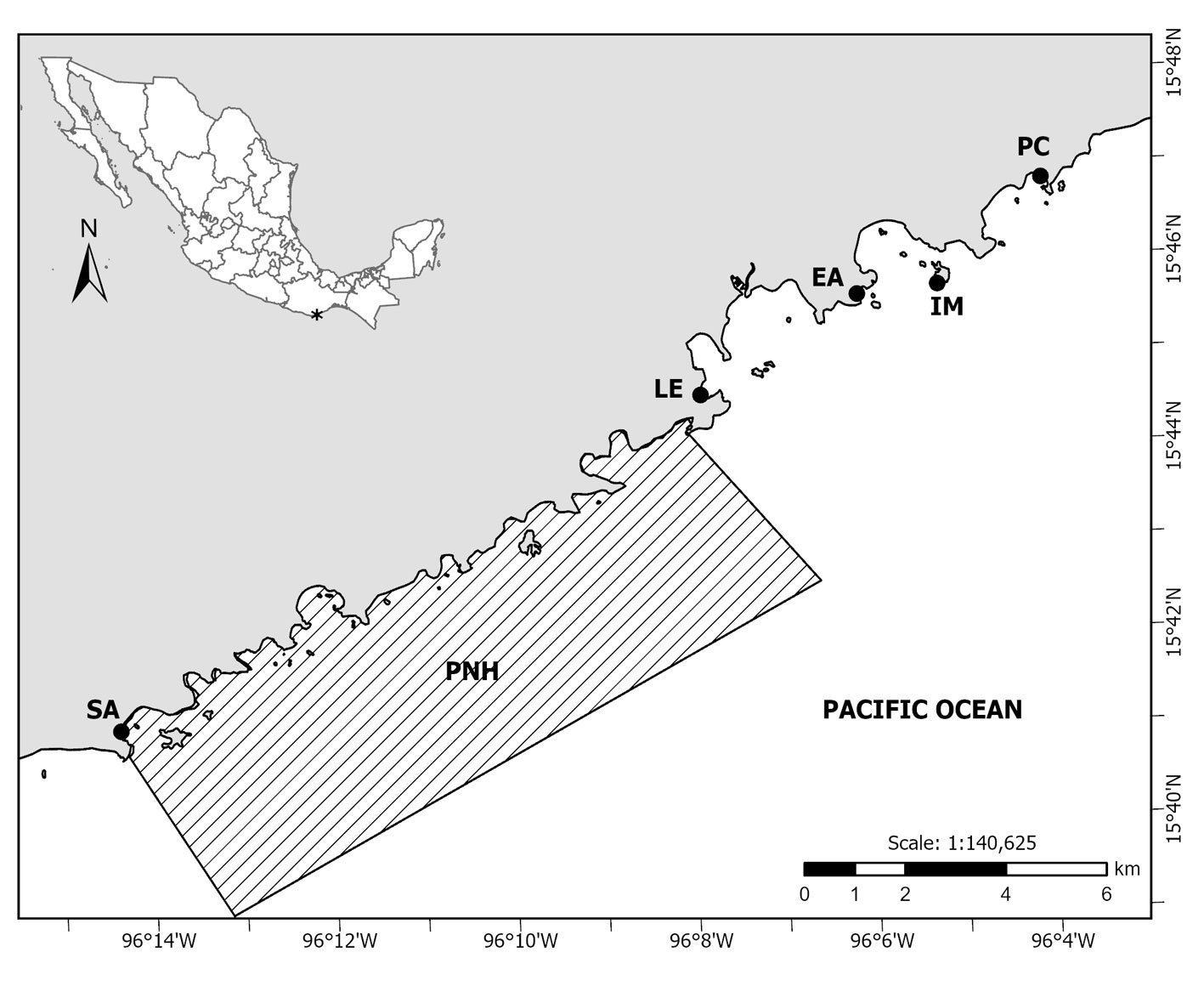
Figure 1. Localities in Bahías de Huatulco (black dots) where this study was held. San Agustín (SA); La Entrega (LE); El Arrocito (EA); Isla Montosa (IM); Playa Conejos (PC). The area belonging to the marine part of the Parque Nacional Huatulco (PNH) is shown in the hatched polygon. Map by O.I. González-Romero.
Table 1
Collecting sites in Bahías de Huatulco: San Agustín, La Entrega, El Arrocito, Isla Montosa, Playa Conejos. Sampling technique: snorkelling (S), scuba diving (SD).
| Locality | Latitude (N) | Longitude (W) | Sampling technique | Substrate composition |
| San Agustín | 15°41.185’ | 96°14.254’ | S | Compact coral colonies, rocks and dead coral patches |
| La Entrega | 15°44.642’ | 96°07.732’ | S, SD | Compact coral colonies, rocks, algae and dead coral patches |
| El Arrocito | 15°45.672’ | 96°06.008’ | S, SD | Rocks with algal turf, coral, sponges and dead coral patches |
| Isla Montosa | 15°45.725’ | 96°05.120’ | SD | Boulders, sand and corals |
| Playa Conejos | 15°46.722’ | 96°03.853’ | S | Boulders, sand and corals |
Results
A total of 298 specimens belonging to 49 species (38 determined to species level, 10 to genus and 1 to family) were recorded from 5 localities in Bahías de Huatulco; the species were distributed in 22 families and 6 orders/superorders. Nudibranchia had the highest number of species (27), followed by Sacoglossa (10), Aplysiida (6), Pleurobranchida (3), and Cephalaspidea (2), while Umbraculida was represented only by 1 species. A list of the sea slugs recorded from Bahías de Huatulco in this study, complemented with the previous records from Oaxaca, is given in Table 2.
Class Gastropoda Cuvier, 1795
Subclass Heterobranchia Gray, 1840
Infraclass Euthyneura Spengel, 1881
Cohort Ringipleura Kano, Brenzinger, Nützel, Wilson and Schrödl, 2016
Subcohort Nudipleura Wägele and Willan, 2000
Order Pleurobranchida Pelseneer, 1906
Family Pleurobranchidae Gray, 1827
Berthellina ilisima Ev. Marcus and Er. Marcus, 1967
(Fig. 2A)
Material examined: 1 organism (18 mm), Entrega (CNMO8025).
Distribution: from Santa Barbara, California to Islas Galapagos, Ecuador (Behrens et al., 2022).
Remarks: animals with nocturnal habits and spongivorous diet (Valdés, 2019).
Berthella sp.
(Fig. 2B)
Material examined: 2 organisms (5, 8 mm), Arrocito (CNMO8274).
Distribution: El Arrocito, Bahías de Huatulco, Oaxaca (this study).
Diagnosis: translucent whitish body with numerous small opaque white dots and low rounded brown tubercles on the dorsum. Small translucent internal shell. The foot protrudes posteriorly from the mantle. The oral velum is triangular and the rolled rhinophores are partially fused.
Remarks: organisms were found under rocks near white sponges. The observed characters in the specimens allowed their identification only to the genus level. Berthella andromeda, B. strongi and B. martensi are also distributed in the Pacific east coast; however, our specimens had a more translucent and white body than B. strongi and they did not present the opaque white transverse bar of B. andromeda (Ghanimi et al., 2020); the dots on the notum also were darker and more regular compared with B. martensi, which has a band along the edge of the mantle (Behrens et al., 2022).
Pleurobranchus digueti Rochebrune, 1895
(Fig. 2C)
Material examined: 3 organisms (15-20 mm), Entrega (CNMO8020); 1 organism (35 mm), Arrocito (CNMO8006); 1 organism (10 mm), Montosa (CNMO7965).
Distribution: from Santa Barbara, California to Islas Galapagos, Ecuador (Behrens et al., 2022).
Remarks: nocturnal animals hide under rocks during the day (Valdés, 2019).
Order Nudibranchia Cuvier, 1817
Family Dorididae Rafinesque, 1815
Dorididae sp.
(Fig. 2D)
Material examined: 1 organism (6 mm), Conejos (CNMO8261).
Distribution: Playa Conejos, Bahías de Huatulco, Oaxaca (this study).
Diagnosis: yellowish body, with an oval orange-brownish patch covering the dorsum and divided by a cream-whitish band that runs through the middle of the rhinophores all the way to the branchial area. The lamellated rhinophores and the gills are the same colour as the body.
Remarks: the specimen was found under rocks at approximately 3 m depth. The observed characters in the organism did not resemble any recorded species in the literature, but they allowed its identification up to the family level.
Doris sp.(Risbec, 1928)
(Fig. 2E)
Material examined: 1 organism (6 mm), Conejos (CNMO8260).
Distribution: Playa Conejos, Bahías de Huatulco, Oaxaca (this study).
Diagnosis: pale yellowish body with discontinued purple band between the rhinophores and the posterior area of the body. The animal had big tubercles in the central area of the dorsum with visible translucent spicules. Rhinophores were lamellated.
Remarks: specimen found on algae of the genus Caulerpa. This specimen resembles the organism illustrated in Behrens et al. (2022) as Doris immonda; however, the previous authors mention that this identification might not be valid due to its geographical distribution, as D. immonda was originally described for the Indo-Pacific. Also, the diagnosis of D. immonda in Gosliner et al. (2018) does not mention the purple band observed in this individual, these authors described a white opaque marking across the body instead. Therefore, we decided to include this species as Doris sp. until a further review of this taxon is made.
Family Discodorididae Bergh, 1891
Diaulula nayarita (Ortea & Llera, 1981)
(Fig. 2F)
Material examined: 1 organism (4 mm), Arrocito (CNMO7974).
Distribution: from Punta Eugenia, Baja California to Panama (Camacho-García et al., 2005).
Remarks: found under rocks near sponges of the same colour as the specimen.
Discodoris ketos (Marcus & Marcus, 1967)
(Fig. 2G)
Material examined: 1 organism (8 mm), Arrocito (CNMO8028).
Distribution: Gulf of California. Mexico to Islas Galapagos, Ecuador (Behrens et al., 2022).
Remarks: it is still unclear whether this species is the same as the circumtropical species Tayuva lilacina (Behrens et al., 2022). Discodoris ketos has a highly specialised diet, feeding on the sponge Haliclona caerulea (Verdín-Padilla et al., 2010).
Geitodoris mavis (Marcus & Marcus, 1967)
(Fig. 2H)
Material examined: 1 organism (15 mm), Entrega (CNMO7964). 1 organism (13 mm), Arrocito (CNMO8029).
Distribution: from Rosarito, Baja California to Islas Galapagos, Ecuador (Behrens et al., 2022).
Remarks: live specimens darkened their gills when disturbed.
Family Polyceridae Alder and Hancock, 1845
Polycera anae Pola et al., 2014
(Fig. 2I)
Material examined: 2 organisms (8, 10 mm), Conejos (CNMO7981).
Distribution: from Mexico to Costa Rica (Pola et al., 2014).
Remarks: found on algae of the genus Padina. Specimens found in this work exceed the maximum length of 5 mm reported for the species by Pola et al. (2014).
Polycera cf. hedgpethi Er. Marcus, 1964
(Fig. 2J)
Table 2
Sea slug fauna recorded from Oaxaca state based on this study and the literature. Localities: Puerto Ángel (PA), San Agustín (SA), El Maguey (EM), La Entrega (LE), El Arrocito (EA), Isla Montosa (IM), Playa Conejos (PC), Santa Cruz (SC), Not available data (ND). New records for the state (*). Only determined species in literature were included. References: 1Holguín-Quiñones and González-Pedraza (1989); 2Rodríguez-Palacios et al. (1988); 3Zamora-Silva and Naranjo-García (2008); 4Barrientos-Luján et al. (2021); 5This study.
| Family | Species | PA | SA | EM | LE | EA | IM | PC | SC | ND | Reference |
| Pleurobranchidae | Berthellina ilisima* | • | 5 | ||||||||
| Berthella sp. | • | 5 | |||||||||
| Pleurobranchus digueti* | • | • | • | 5 | |||||||
| Dorididae | Dorididae sp. | • | 5 | ||||||||
| Doris sp. | • | 5 | |||||||||
| Discodorididae | Diaulula nayarita* | • | 5 | ||||||||
| Diaulula sandiegensis | • | 2 | |||||||||
| Discodoris ketos* | • | 5 | |||||||||
| Geitodoris mavis* | • | • | 5 | ||||||||
| Polyceridae | Polycera anae* | • | 5 | ||||||||
| Polycera cf. hedgpethi* | • | 5 | |||||||||
| Tambja abdere* | • | 5 | |||||||||
| Chromodorididae | Felimida sphoni* | • | • | • | 5 | ||||||
| Chromolaichma dalli* | • | • | • | 5 | |||||||
| Chromolaichma sedna* | • | • | 5 | ||||||||
| Felimare agassizii* | • | • | • | • | 5 | ||||||
| Cadlinidae | Cadlina sp. | • | • | • | 5 | ||||||
| Dendrodorididae | Dendrodoris krebsii | • | 2 | ||||||||
| Doriopsilla janaina* | • | • | • | 5 | |||||||
| Tritoniidae | Tritonia festiva | • | 2 | ||||||||
| Hancockiidae | Hancockia californica* | • | 5 | ||||||||
| Flabellinidae | Coryphellina marcusorum* | • | 5 | ||||||||
| Samla telja* | • | • | • | • | 5 | ||||||
| Cuthonidae | Cuthona divae | • | 2 | ||||||||
| Cuthona sp. 1 | • | 5 | |||||||||
| Cuthona sp. 2 | • | 5 | |||||||||
| Aeolidiidae | Bulbaeolidia sulphurea* | • | 5 | ||||||||
| Anteaeolidiella chromosoma* | • | • | 5 | ||||||||
| Anteaeolidiella ireneae* | • | 5 | |||||||||
| Baeolidia moebii* | • | 5 | |||||||||
| Limenandra confusa* | • | • | 5 | ||||||||
| Spurilla braziliana* | • | 5 | |||||||||
| Facelinidae | Favorinus elenalexiarum* | • | • | 5 | |||||||
| Phidiana lascrucensis* | • | • | • | • | • | 5 | |||||
| Tylodinidae | Tylodina fungina* | • | 5 | ||||||||
| Table 2. Continued | |||||||||||
| Bullidae | Bulla punctulata | • | 1 | ||||||||
| Bulla gouldiana | • | 4 | |||||||||
| Haminoeidae | Haminoea sp. | • | • | 5 | |||||||
| Aliculastrum exaratum | • | 4 | |||||||||
| Aglajidae | Navanax aenigmaticus* | • | • | • | 5 | ||||||
| Aplysiidae | Aplysia cf. cedrosensis* | • | 5 | ||||||||
| Aplysia californica | • | 2 | |||||||||
| Aplysia hooveri* | • | • | • | • | 5 | ||||||
| Dolabella cf. auricularia* | • | • | 5 | ||||||||
| Dolabella californica | • | 2 | |||||||||
| Dolabrifera nicaraguana* | • | 5 | |||||||||
| Phyllaplysia padinae* | • | 5 | |||||||||
| Stylocheilus rickettsi* | • | • | 5 | ||||||||
| Oxynoidae | Lobiger cf. souverbii* | • | • | 5 | |||||||
| Oxynoe aliciae* | • | 5 | |||||||||
| Plakobranchidae | Elysia diomedea | • | • | • | • | • | 3, 5 | ||||
| Elysia cf. pusilla* | • | • | 5 | ||||||||
| Elysia sp. 1 | • | • | • | 5 | |||||||
| Elysia sp. 2 | • | • | • | • | 5 | ||||||
| Limapontiidae | Placida cf. dendritica* | • | 5 | ||||||||
| Hermaeidae | Polybranchia mexicana* | • | 5 | ||||||||
| Caliphylla sp. | • | 5 | |||||||||
| Hermaea sp. | • | 5 | |||||||||
| Total | 3 | 14 | 1 | 25 | 27 | 10 | 18 | 1 | 3 |

Figure 2. New records of sea slugs for Oaxaca. A, Berthellina ilisima; B, Berthella sp.; C, Pleurobranchus digueti; D, Dorididae sp. 1; E, Doris sp.; F, Diaulula nayarita; G, Discodoris ketos; H, Geitodoris mavis; I, Polycera anae; J, Polycera cf. hedgpethi. Scale bar = 5mm. Photos by O.I. González-Romero.
Material examined: 1 organism (14 mm), Montosa. Photographic record only.
Distribution: from Puerto Peñasco, Mexico to Islas Galapagos, Ecuador (Behrens et al., 2022).
Remarks: found on rocks with bryozoan colonies. Behrens et al. (2022) treat this species as Polycera gnupa; however, it is unclear if this nudibranch is different from the widespread species P. hedgpethi.
Tambja abdere Farmer, 1978
(Fig. 3A)
Material examined: 1 organism (42 mm), Montosa (CNMO7966).
Distribution: from the Gulf of California, Mexico to Costa Rica (Behrens et al., 2022).
Remarks: the specimen was found on rocks at approximately 13 m depth. According to Hermosillo (2007), T. abdere feeds on the bryozoan Sessibugula translucens which lives in zones with low currents.
Family Chromodorididae Bergh, 1891
Felimida sphoni Ev. Marcus, 1971
(Fig. 3B)
Material examined: 1 organism (5 mm), Entrega (CNMO8270). Three organisms (8-14 mm), Arrocito (CNMO8262, CNMO8272). Three organisms (9-12 mm), Conejos (CNMO8263, CNMO8265).
Distribution: from the Gulf of California, Mexico to Ecuador (Behrens et al., 2022).
Remarks: animals were found under rocks near to different unidentified sponges.
Chromolaichma dalli (Bergh, 1879)
(Fig. 3C)
Material examined: 5 organisms (17-32 mm), Montosa (CNMO8259). One organism (5 mm), Conejos (CNMO8264).
Distribution: from Islas San Benito, Baja California to Islas Galapagos, Ecuador (Behrens et al., 2022).
Remarks: larger specimens were found at approximately 15 m depth. Matsuda and Gosliner (2018) categorized C. dalli under a temporal nomenclatural name that needs further taxonomic analysis.
Chromolaichma sedna (Ev. Marcus & Er. Marcus, 1967)
(Fig. 3D)
Material examined: 1 organism (31 mm), Montosa (CNMO8278).
Distribution: from the Gulf of California, Mexico to Ecuador (Behrens et al., 2022).
Remarks: Verdín-Padilla et al. (2010) reported that C. sedna is a polyphagous species that may feed on 16 sponge species.
Felimare agassizii (Bergh, 1894)
(Fig. 3E)
Material examined: 2 organisms (9, 32 mm), Entrega (CNMO8276, CNMO8281). Four organisms (32-55 mm), Arrocito (CNMO8279, CNMO8280, CNMO8282, CNMO8283). One organism (14 mm), Montosa (CNMO8275).
Distribution: from the Gulf of California, Mexico to Islas Galapagos, Ecuador (Behrens et al., 2022).
Remarks: Verdín-Padilla et al. (2010) reported that F. agassizii has a polyphagous diet feeding on 9 sponge species.
Family Cadlinidae Bergh, 1891
Cadlina sp.
(Fig. 3F)
Material examined: 5 organisms (4-5 mm), Entrega. One organism (3 mm), Arrocito. Two organisms (4 mm), Conejos. Photographic record only.
Distribution: from Baja California, Mexico to Panama (Behrens et al., 2022).
Diagnosis: oval translucent white body with 4-5 rounded yellow glands around the mantle at each side of the body, simulating an inner semi-oval. The rhinophores are white with a red band in the centre.
Remarks: the specimens were found on white sponges. Specimens resemble Cadlina sp. in Camacho-García et al. (2005), Bertsch and Aguilar Rosas (2016) and Behrens et al. (2022). This undescribed species has been reported in several locations for the Pacific east coast such as Islas Tres Marías (Hermosillo, 2009), Revillagigedo (Hermosillo & Gosliner, 2008), Bahía de Banderas (Hermosillo, 2011), Acapulco (Flores-Rodríguez et al., 2017) and Costa Rica (Camacho-García et al., 2005).
Family Dendrodorididae O’Donoghue, 1924 (1864)
Doriopsilla janaina Er. Marcus and Ev. Marcus, 1967
(Fig. 3G)
Material examined: 1 organism (18 mm), Entrega (CNMO8022). Two organisms (13, 28 mm), Conejos (CNMO8014, CNMO7985).
Distribution: from Baja California, Mexico to Islas Galapagos, Ecuador (Behrens et al., 2022).
Remarks: 1 specimen was found on brown algae. Although there are reports of the gregarious behaviour of these animals (Hermosillo et al., 2006), they were found individually in our surveys.
Suborder Cladobranchia
Family Hancockiidae MacFarland, 1923
Hancockia californica MacFarland, 1923
(Fig. 3H)
Material examined: 3 organisms (5-11 mm), Arrocito (CNMO7968).
Distribution: from Big Lagoon, California to Costa Rica (Behrens et al., 2022).
Remarks: the specimens were found on green algae. Even though the 3 specimens were collected on the same algae, they presented colour variations in their bodies, from transparent brown to reddish-brown.
Family Flabellinidae Bergh, 1889
Coryphellina marcusorum (Gosliner & Kuzirian, 1990)
(Fig. 3I)
Material examined: 6 organisms (6-18 mm), Montosa (CNMO7976).
Distribution: from Isla San Diego, Baja California to Islas Galapagos, Ecuador (Behrens et al., 2022).
Remarks: specimens were observed at more than 15 m depth. Animals feed on hydroids of the genus Eudendrium (Camacho-García et al., 2005).
Samla telja (Ev. Marcus & Er. Marcus, 1967)
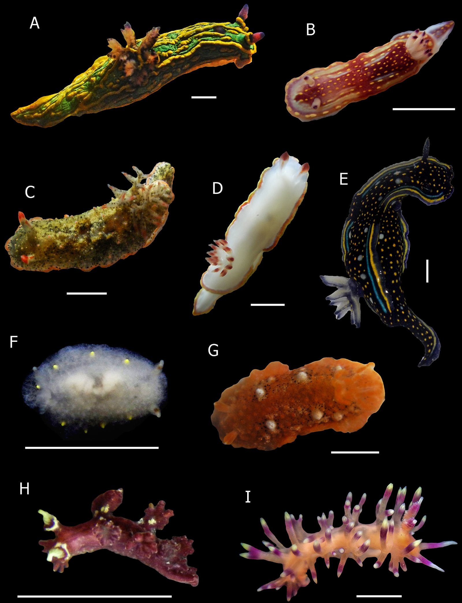
Figure 3. New records of sea slugs for Oaxaca. A, Tambja abdere; B, Felimida sphoni; C, Chromolaichma dalli; D, Chromolaichma sedna; E, Felimare agassizii; F, Cadlina sp; G, Doriopsilla janaina; H, Hancockia californica; I, Coryphellina marcusorum. Scale bar = 5 mm. Photos by O.I. González-Romero.
(Fig. 4A)
Material examined: 1 organism (9 mm), Arrocito (CNMO7971). One organism (8 mm), Montosa (CNMO7967).
Distribution: from Puerto Peñasco, Mexico to Islas Galapagos, Ecuador (Behrens et al., 2022).
Remarks: organisms found on hydroids during daytime as reported by Behrens (2022).
Family: Cuthonidae Odhner, 1934
Cuthona sp. 1
(Fig. 4B)
Material examined: 1 organism (3 mm), Arrocito. Photographic record only.
Distribution: from Puerto Vallarta, Mexico to Islas Catalinas, Costa Rica (Camacho-García et al., 2005).
Diagnosis: translucent whitish body with several opaque white spots. The cerata are globose and have longitudinal yellowish lines with a reddish colour on the base. The smooth rhinophores and the oral tentacles are white coloured on the tips and have a reddish-brown band on the base.
Remarks: juvenile specimen found on hydroids with S. telja individuals. Our species diagnosis match Cuthona sp. 3 in Camacho-García et al. (2005). Before this work, this undescribed species had been reported only in 2 localities that correspond to its geographic distribution limits.
Cuthona sp. 2
(Fig. 4C)
Material examined: 1 organism (5 mm), Agustín. Photographic record only.
Distribution: San Agustín, Bahías de Huatulco, Oaxaca (this study).
Diagnosis: light orange body with multiple little white spots. The pericardial area is swollen and has a distinctive white patch. The cerata colour base is brown with several little yellow dots. The smooth rhinophores have orange freckles and an orange band near the tips. The oral tentacles are shorter than the rhinophores and have 2 distinctive orange bands, 1 on the base and the other near the centre.
Remarks: the animal was found near egg masses, possibly just laid by the observed specimen. The observed characters in the organism allowed its identification only to the genus level. Specimen diagnosis did not match any recorded species in the literature.
Family Aeolidiidae Gray, 1827
Bulbaeolidia sulphurea Caballer and Ortea, 2015
(Fig. 4D)
Material examined: 4 organisms (4-12 mm), Agustín (CNMO7975, CNMO7995, CNMO8001).
Distribution: from Puerto Vallarta, Mexico to Islas Galapagos, Ecuador (Behrens et al., 2022).
Remarks: 1 specimen was found on green algae. This species feeds on anemones (Behrens et al., 2022).
Anteaeolidiella chromosoma (Cockerell & Eliot, 1905)
(Fig. 4E)
Material examined: 8 organisms (15-22 mm), Agustín (CNMO7973, CNMO8002, CNMO8005).
Distribution: from Morro Bay, California to Islas Galapagos, Ecuador (Camacho-García et al., 2005).
Remarks: specimens were found under rocks and near coral polyps.
Anteaeolidiella ireneae Carmona et al., 2014
(Fig. 4F)
Material examined: 1 organism (21 mm), Entrega (CNMO8017).
Distribution: from Isla Socorro, Mexico to Panama (Carmona et al., 2014a).
Remarks: feeds on anemones (Behrens et al., 2022).
Baeolidia moebii Bergh, 1888
(Fig. 4G)
Material examined: 1 organism (27 mm), Agustín. Photographic record only.
Distribution: from the Gulf of California, Mexico to Panama (Hermosillo et al., 2006).
Remarks: found under bivalve shells in shallow water (2 m).
Limenandra confusa Carmona et al., 2014
(Fig. 4H)
Material examined: 2 organisms (16, 18 mm), Arrocito (CNMO8033).
Distribution: from the Gulf of California, Mexico to Costa Rica (Carmona et al., 2014c).
Remarks: Carmona et al. (2014c) report that this species feeds on small anemones.
Spurilla braziliana MacFarland, 1909
(Fig. 4I)
Material examined: 1 organism (24 mm), Arrocito. Photographic record only.
Distribution: from Baja California Sur, Mexico to Colombia (Behrens et al., 2022).
Remarks: Carmona et al. (2014b) confirmed that S. braziliana is a widespread species and its presence in the Pacific east coast is probably due to human introduction.
Family Facelinidae Bergh, 1889
Favorinus elenalexiarum García and Troncoso, 2001

Figure 4. New records of sea slugs for Oaxaca. A, Samla telja; B, Cuthona sp. 1; C, Cuthona sp. 2; D, Bulbaeolidia sulphurea; E, Anteaeolidiella chromosoma; F, Anteaeolidiella ireneae; G, Baeolidia moebii; H, Limenandra confusa; I, Spurilla braziliana. Scale bar = 5mm. Photos by O.I. González-Romero.
(Fig. 5A)
Material examined: 1 organism (4 mm), Entrega. 1 organism (12 mm), Arrocito. Photographic record only.
Distribution: from the Gulf of California, Mexico to Islas Galapagos, Ecuador (Behrens et al., 2022).
Remarks: specimens found near Aplysia egg masses.
Phidiana lascrucensis Bertsch and Ferreira, 1974
(Fig. 5B)
Material examined: 1 organism (9 mm), Entrega (CNMO7998). Two organisms (8, 12 mm), Arrocito (CNMO7969, CNMO8003). One organism (24 mm), Montosa (CNMO8036). Five organisms (10-21 mm), Conejos (CNMO7980, CNMO8035).
Distribution: from Baja California, Mexico to Panama (Behrens et al., 2022).
Remarks: organisms found under rocks, often observed near specimens of Chiton albolineatus.
Cohort Tectipleura Schrödl, Jörger, Klussmann-Kolb and Wilson, 2011
Subcohort Euopisthobranchia Jörger, Stöger, Kano, Fukuda, Knebelsberger and Schrödl, 2010
Order Umbraculida, Odhner, 1939
Family Tylodinidae Gray, 1847
Tylodina fungina Gabb, 1865
(Fig. 5C)
Material examined: 2 organisms (6, 8 mm), Arrocito (CNMO7994, CNMO8030).
Distribution: from Baja California, Mexico to Islas Galapagos, Ecuador (Hermosillo et al., 2006).
Remarks: Tylodina fungina has a highly specialist diet, feeding on the sponge Aiolochroia thiona and Aplysina gerardogreeni (Behrens et al., 2022; Verdín-Padilla et al., 2010).
Order Cephalaspidea Fischer, 1883
Family Haminoeidae Pilsbry, 1895
Haminoea sp.
(Fig. 5D)
Material examined: 2 organisms (8, 10 mm), Arrocito (CNMO7958).
Distribution: from Bahía de Banderas, Mexico to Peru (Behrens et al., 2022).
Diagnosis: body oval. White cream body, with irregular dark brown patches. The animals have an inverted “V” stain in the cephalic area between the eyes. The body is surrounded by multiple orange and light brown dots.
Remarks: specimens found on marine brown cyanobacteria. This species was firstly identified as the Indo-Pacific species Lamprohaminoea ovalis by Valdés and Camacho-García (2004). However, recently phylogenetic analysis has shown that the specimens in the Pacific east coast are an undescribed species more related to the Atlantic and Pacific species of the genus Haminoea (Oskars & Malaquias, 2019, 2020).
Family Aglajidae Pilsbry, 1895
Navanax aenigmaticus (Bergh, 1893)
(Fig. 5E)
Material examined: 5 organisms (30-44 mm), Entrega (CNMO7996, CNMO7999, CNMO8007). Two organisms (21, 33 mm), Arrocito (CNMO8032).
Distribution: from Baja California, Mexico to Chile (Behrens et al., 2022).
Remarks: collected specimens presented different body colour variations from black, brown, and pink with cream or whitish spots. According to Ornelas-Gatdula et al. (2012), colouration differences on N. aenigmaticus could be probably influenced by environmental factors.
Order Aplysiida
Family Aplysiidae Lamarck, 1809
Aplysia cf. cedrosensis
(Fig. 5F)
Material examined: 1 organism (22 mm), Conejos (CNMO7978).
Distribution: from Bahía de los Angeles, Baja California to Playa Conejos, Bahías de Huatulco, Oaxaca.
Remarks: juvenile specimen found under rocks near red algae. Our diagnosis matched the species A. cedrosensis in Hermosillo et al. (2006). However, Behrens et al. (2022) state that this species might be a synonym of the California black sea hare Aplysia vaccaria. Before this work, the southern distribution of A cedrosensis in the Pacific east coast was reported for Parque de la Reina, Acapulco (Flores-Rodríguez et al., 2017), approximately 440 km northeast from Playa Conejos, Oaxaca.
Aplysia hooveri Golestani et al., 2019
(Fig. 5G)
Material examined: 72 organisms (3-16 mm), Entrega (CNMO7961-7963, CNMO7986, CNMO8010, CNMO8021, CNMO8026, CNMO8034). Two organisms (6, 7 mm), Arrocito (CNMO7972). Five organisms (5-12 mm), Conejos (CNMO7982, CNMO7993).
Distribution: from Baja California, Mexico to Islas Galapagos, Ecuador (Valdés, 2019).
Remarks: this species was highly abundant in some localities of the study area; it was usually associated with red and brown algae.
Dolabella cf. auricularia (Lightfoot, 1786)
(Fig. 5H)
Material examined: 1 organism (180 mm), Agustín. One organism (210 mm), Entrega. Photographic record only.
Distribution: from the Gulf of California, Mexico to Ecuador (Zamora-Silva & Naranjo-García, 2008).
Remarks: found on algae at approximately 10 m depth. According to Behrens et al. (2022) there is molecular evidence that confirms that Dolabella auricularia is a species complex.
Dolabrifera nicaraguana Pilsbry, 1896
(Fig. 5I)

Figure 5. New records of sea slugs for Oaxaca. A, Favorinus elenalexiarum; B, Phidiana lascrucensis; C, Tylodina fungina; D, Haminoea sp.; E, Navanax aenigmaticus; F. Aplysia cf. cedrosensis; G, Aplysia hooveri; H, Dolabella cf. auricularia; I, Dolabrifera nicaraguana. Scale bar = 5 mm. Photos by O.I. González-Romero.
Material examined: 1 organism (14 mm), Entrega (CNMO7960).
Distribution: from Bahía de las Cruces, Baja California to Tumbes, Peru (Valdés et al., 2018).
Remarks: cryptic specimen found on rhodolith beds.
Phyllaplysia padinae Williams and Gosliner, 1973
(Fig. 6A)
Material examined: 4 organisms (8-18 mm), Conejos (CNMO8277, CNMO8268, CNMO8269).
Distribution: from the Gulf of California, Mexico to Islas Galapagos, Ecuador (Camacho-García et al., 2005).
Remarks: the specimens were found attached to algae of the genera Padina and Caulerpa.
Stylocheilus rickettsi (MacFarland, 1966)
(Fig. 6B)
Material examined: 29 organisms (5-29 mm), Entrega (CNMO7959, CNMO7997, CNMO8008, CNMO8018, CNMO8023, CNMO8024, CNMO8027). Five organisms (6-38 mm), Arrocito (CNMO7957, CNMO7970).
Distribution: from Baja California, Mexico to Islas Galapagos, Ecuador (Bazzicalupo et al., 2020).
Remarks: the specimens were found on rocks and on different unidentified green, red, and brown algae.
Subcohort Panpulmonata Jörge et al., 2010
Superorder Sacoglossa Ihering, 1876
Family Oxynoidae Stoliczka, 1868 (1847)
Lobiger cf. souverbii Fischer, 1857
(Fig. 6C)
Material examined: 1 organism (6 mm), Entrega (CNMO8015). One organism (9 mm), Conejos (CNMO7983).
Distribution: Baja California Sur, Mexico to Islas Galapagos, Ecuador (Behrens et al., 2022).
Remarks: specimens were found associated with algae of the genus Caulerpa as mentioned in the literature (Behrens et al., 2022; Camacho-García et al., 2005). Due to the original description of L. souverbii in the Caribbean region, this sacoglossan is suspected to be a different species.
Oxynoe aliciae Krug et al., 2018
(Fig. 6D)
Material examined: 6 organisms (4-9 mm), Entrega (CNMO8009, CNMO8016).
Distribution: from Baja California Sur, Mexico to Islas Galapagos, Ecuador (Behrens et al., 2022).
Remarks: specimens found as hosts on the algae Caulerpa as mentioned by Krug et al. (2018).
Family Plakobranchidae Gray, 1840
Elysia cf. pusilla (Bergh, 1871)
(Fig. 6E)
Material examined: 3 organisms (8-11 mm), Arrocito (CNMO8004). Ten organisms (8-10 mm), Conejos (CNMO7977, CNMO8000, CNMO8013).
Distribution: from Mexico to Costa Rica (Behrens et al., 2022).
Remarks: cryptic specimens were found attached to algae of the genus Halimeda as mentioned in the literature (Behrens et al., 2022; Camacho-García et al., 2005). This species is presumed to be different from E. pusilla, which was originally described in the Indo-Pacific region (Behrens et al., 2022).
Elysia sp. 1
(Fig. 6F)
Material examined: 4 organisms (6-10 mm), Arrocito. Twenty-seven organisms (5-14 mm), Conejos. Photographic record only.
Distribution: from Bahía de Banderas, Mexico to Panama (Hermosillo et al., 2006).
Diagnosis: elongated olive-greenish body. The rolled rhinophores are yellow whitish with light brown patches. The parapodia are strongly folded with an opening in the centre. Some specimens have a white spot in the base of the rhinophores.
Remarks: specimens were found associated with algae of the genus Halimeda. Our diagnosis resembles the species Elysia sp. 1 in Camacho-García et al. (2005) and Hermosillo et al. (2006). There are numerous records of this undescribed species in the Pacific east coast: Bahía de Banderas (Hermosillo, 2011), Ixtapa, Guerrero (Hermosillo & Behrens, 2005), Papagayo and Parque de la Reina, Acapulco (Flores-Rodríguez et al., 2017), Playa Avellanas and San Pedrillo, Costa Rica (Camacho-García et al., 2005) and Panama (Hermosillo et al., 2006).
Elysia sp. 2
(Fig. 6G)
Material examined: 4 organisms (13-24 mm), Entrega. Two organisms (19, 22 mm), Arrocito. 8 organisms (12-24 mm), Conejos. Photographic record only.
Distribution: from Islas Revillagigedo, Mexico to Costa Rica (Behrens et al., 2022).
Diagnosis: elongated light-greenish body with several white and dark green specks. The rhinophores are smooth, large, and rolled. The convoluted parapodia are folded with several rounded whitish papillae on the edges. Adult specimens have a purple-pinkish colouration along the margin of the parapodia and in the basis of the rhinophores.
Remarks: some specimens were found on red and green algae of the genus Halimeda and Caulerpa. Our diagnosis matched the species Elysia sp. 2 in Camacho-García et al. (2005) and Elysia sp. in Behrens et al. (2022). This undescribed species was previously documented in multiple locations in the Pacific east coast: Bahía de Banderas (Hermosillo, 2011), Islas Revillagigedo (Hermosillo & Gosliner, 2008), Isla Clipperton (Kaiser, 2007), Ixtapa, Guerrero (Hermosillo & Behrens, 2005) and Costa Rica (Camacho-García et al., 2005).
Family Limapontiidae Gray, 1847
Placida cf. dendritica (Alder and Hancock, 1843)
(Fig. 6H)
Material examined: 3 organisms (3-5 mm), Entrega (CNMO8019).
Distribution: from the Gulf of California to La Entrega, Bahías de Huatulco, Oaxaca.
Remarks: specimens were found on algae of the genus Bryopsis. Before this work, the southern distribution of P. dendritica in the Pacific east coast was known for Bahía de Banderas, Nayarit (Hermosillo, 2011), approximately 1,200 km northeast from La Entrega, Oaxaca. It is suspected that P. dendritica might be a species complex that encompasses 2 different species in the region (Behrens et al., 2022).
Family Hermaeidae H. Adams and A. Adams, 1854
Polybranchia mexicana Medrano et al., 2018
(Fig. 6I)
Material examined: 1 organism (48 mm), Conejos (CNMO7992).
Distribution: from Baja California, Mexico to Islas Galapagos, Ecuador (Medrano et al., 2018).
Remarks: specimen found under rocks at daylight supporting the reports of the nocturnal habits of the species (Behrens et al., 2022).
Caliphylla sp.
(Fig. 6J)
Material examined: 4 organisms (5-14 mm), Entrega. Photographic record only.
Distribution: from La Entrega, Mexico to Islas Galapagos, Ecuador.
Diagnosis: elongated translucent green body with multiple little dark green and white dots. The bifid rhinophores, the head and the cerata have visible dark green ramified digestive branches. The elongated cerata are flattened and pointed. Some specimens may have a white speck between the eyes and in the posterior part of the head.
Remarks: some specimens were found on algae of the genus Bryopsis. Our diagnosis coincides with the undescribed species Caliphylla sp. in Camacho-García et al. (2005), which has been previously reported in a few localities from Costa Rica and Ecuador.
Hermaea sp.
(Fig. 6K)
Material examined: 1 organism (5 mm), Entrega. Photographic record only.
Distribution: from La Entrega, Oaxaca, Mexico to Playa Real, Guanacaste, Costa Rica.
Diagnosis: cream coloured body with multiple dark green flecks. Rhinophores are auriculate. The arrow-head shape cerata are covered with several white dots and red-brownish ramified digestive branches are visible throughout.
Remarks: the specimen was found on filamentous red algae. Our diagnosis resembles the species Hermaea sp. 3 in Camacho-García et al. (2005), which has been previously reported in Costa Rica.

Figure 6. New records of sea slugs for Oaxaca. A, Phyllaplysia padinae; B, Stylocheilus rickettsi; C, Lobiger cf. souverbii; D, Oxynoe aliciae; E, Elysia cf. pusilla; F, Elysia sp. 1; G, Elysia sp. 2; H, Placida cf. dendritica; I, Polybranchia mexicana; J, Caliphylla sp.; K, Hermaea sp. Scale bar = 5 mm. Photos by O.I. González-Romero.
Discussion
In this study we added 48 sea slug records, increasing by 83% the knowledge of sea slugs’ diversity for Oaxaca, from 10 to 58 species (Table 2). Also, the records presented in this study represent almost 11% of the total sea slug species previously known for the Eastern Pacific, from Alaska to Peru (Behrens et al., 2022). Among the sea slug fauna from Oaxaca, the order Nudibranchia is the most diverse encompassing more than half of the registered species, which is a general trend observed worldwide and in other localities from the Tropical Eastern Pacific (TEP) (García-Méndez & Camacho-García, 2016; Gosliner, 1991; Hermosillo, 2004; Spalding et al., 2007), and might be explained due to phylogenetic, historical and functional variables within the group (Bertsch, 2010). In contrast with other localities on the Pacific coast of Mexico (Table 3), the total number of species recorded in Oaxaca is similar to those reported for Isla Tres Marías, Nayarit (52 spp.), which is a relatively lower species richness compared with other works that involve higher sampling effort and/or more extensive study areas (Angulo-Campillo, 2005; Bertsch, 2014; Hermosillo, 2011; Hermosillo & Behrens, 2005). Moreover, the percentage of shared species between Revillagigedo, Colima and Oaxaca is higher (57.1%) than in other localities; however, this amount could be inaccurate due to the underestimated sea slug diversity in Islas Revillagigedo pointed out by Hermosillo and Gosliner (2008).
Overall, almost all the new sea slug records in this study are endemic to the Panamic biogeographic province (Briggs & Bowen, 2012), with some exceptions previously remarked that are also distributed on the Western Atlantic and/or the Indo-Pacific regions. Most of these exceptions belong to species complex that have not been resolved yet (Behrens et al., 2022), but others have a widespread natural distribution, or they have been introduced possibly by humans’ influence, as it has been suggested for S. braziliana (Carmona et al., 2014b). Interestingly, all the species previously reported for Oaxaca by Rodríguez-Palacios et al. (1988) (see Table 2) are not distributed in the Panamic province nor any warm waters of the Pacific east coast. Therefore, these records should be treated with caution as these species might have been misidentified due to the lack of specific field guides and accessible literature related with the sea slug fauna for this region in the past.
Coral reef communities, including those inhabiting the TEP, are one of the most thriving habitats for sea slugs, as they encompass a net of biological associations that increase their diversity and inherent productivity (Sanvicente-Añorve et al., 2012; Sreeraj et al., 2013). In general, we found a higher species richness in localities with greater heterogeneity in their substrate composition (Table 1), possibly providing more habitats for sea slugs to succeed in this area. San Agustín, which is inside a Natural Protected Area, did not show a higher species richness compared to other localities. However, the number of species in this locality is underestimated, as we could not perform algae collection as an indirect search method; additionally, other variables need to be analysed to determine whether there is a significant difference in the sea slug diversity between protected and non-protected areas.
The continuous discovery of undescribed sea slug species in the TEP, such as the ones reported in this work: Berthella sp., Dorididae sp., Doris sp., and Cuthona sp. 2 has been a common issue, even in recent years. Phylogenetic and systematic studies have helped to elucidate the status of certain sea slug taxa (e.g., Bazzicalupo et al., 2020; Golestani et al., 2019; Krug et al., 2018; Medrano et al., 2018; Valdés et al., 2018), and represent important efforts to better understand the diversity of the sea slug fauna in the TEP. Nonetheless, there are species recorded more than a decade ago, such as Cadlina sp., Cuthona sp. 1, Elysia sp. 1, Elysia sp. 2, Caliphylla sp. and Hermaea sp. that remain undescribed. In the same way, some studies have found uncertainties in described species related to their geographic distribution. For instance, Behrens et al. (2022) state that Aplysia cf. cedrosensis and Placida cf. dendritica are given names that belong to 2 or more undescribed species that inhabit different biogeographic provinces. The extension of the distribution for those species reported in this work could confirm that they are different species indeed, and further taxonomic studies regarding the description and distribution of each species need to be done.
Table 3
Studies on sea slug diversity from the Pacific coast of Mexico. Shared species refer to those species present in other localities and this study (Huatulco).
| Locality | Number of species | Number of shared species (%) | Reference |
| Bahía de los Angeles, Baja California | 117 | 26 (22.2) | Bertsch (2014) |
| Baja California Sur | 117 | 31 (26.4) | Angulo-Campillo (2005) |
| Bahía de Banderas, Nayarit-Jalisco | 146 | 44 (30.1) | Hermosillo (2011) |
| Islas Tres Marías, Nayarit | 52 | 27 (51.9) | Hermosillo (2009) |
| Revillagigedo, Colima | 42 | 24 (57.1) | Hermosillo and Gosliner (2008) |
| Colima, Michoacán and Guerrero | 76 | 38 (50) | Hermosillo and Behrens (2005) |
| Acapulco, Guerrero | 63 | 27 (42.8) | Flores-Rodríguez et al. (2017) |
This study updates the knowledge of the sea slug fauna of Oaxaca and the southern Pacific coast of Mexico; however, many unexplored localities in this region still need to be studied. Since this region could be a potential hotspot of marine biodiversity (Bastida-Zavala et al., 2013), further efforts to find sea slugs are needed. Future samplings involving SCUBA diving on different habitats such as lagoons, mangroves, and rocky shores at different times of the day may help to increase this inventory. This work also contributes to the biological inventory of Parque Nacional Huatulco, which is essential to determine future perspectives in the conservation planning and management of this and other Natural Protected Areas (Bezaury-Creel & Gutiérrez, 2009).
Acknowledgements
We thank Parque Nacional Huatulco for allowing us the entrance to perform the surveys in the locality of San Agustín; OGR acknowledges Comisión Nacional de Becas de Educación Superior, SEP for the financial support as an undergraduate student; XGV acknowledges Consejo Nacional de Ciencia y Tecnología (Conacyt) her PhD scholarship (CVU: 564148). We thank A. Valdés, P. Krug and S. Medrano, who helped with the identification of some organisms, and E. Naranjo-García for providing a space to work in her laboratory. We thank F. Pérez, M. Pérez, and M. A. Arriaga for their hospitality and support in performing this study; to the staff of “Buceo Anfibios Huatulco” and all the people who helped us in the surveys, especially E. Molina, L. Jiménez, A. García and A. Barrera.
References
Alexander, T. J., Barrett, N., Haddon, M., & Edgar, G. (2009). Relationships between mobile macroinvertebrates and reef structure in a temperate marine reserve. Marine Ecology Progress Series, 389, 31–44. https://doi.org/10.3354/meps08210
Angulo-Campillo, O. (2005). A four-year survey of the opisthobranch fauna (Gastropoda, Opisthobranchia) from Baja California Sur. Vita Malacologica, 3, 43–50.
Barrientos-Luján, N. A., Rodríguez-Zaragoza, F. A., & López-Pérez, A. (2021). Richness, abundance and spatial heterogeneity of gastropods and bivalves in coral ecosystems across the Mexican Tropical Pacific. Journal of Molluscan Studies, 87, eyab004. https://doi.org/10.1093/mollus/eyab004
Bastida-Zavala, J. R., García-Madrigal, M. S., Rosas-Alquicira, E. F., López-Pérez, R. A., Benítez-Villalobos, F., Meraz-Hernando, J. F. et al. (2013). Marine and coastal biodiversity of Oaxaca, Mexico. Check List, 9, 329–390. https://doi.org/10.15560/9.2.329
Bazzicalupo, E., Crocetta, F., Gosliner, T. M., Berteaux-Lecellier, V., Camacho-García, Y. E., Sneha Chandran, B. K. et al. (2020). Molecular and morphological systematics of Bursatella leachii de Blainville, 1817 and Stylocheilus striatus Quoy & Gaimard, 1832 reveal cryptic diversity in pantropically distributed taxa (Mollusca: Gastropoda: Heterobranchia). Invertebrate Systematics, 34, 535–568. https://doi.org/10.1071/IS19056
Behrens, D. W. (2005). Nudibranch behaviour. Jacksonville, FL: New World Publications.
Behrens, D. W., Fletcher, K., Hermosillo, A., & Jensen, G. C. (2022). Nudibranchs and sea slugs of the Eastern Pacific. Bremerton, Washington: MolaMarine.
Benkendorff, K., & Davis, A. R. (2002). Identifying hotspots of molluscan species richness on rocky intertidal reefs. Biodiversity and Conservation, 11, 1959–1973. https://doi.org/10.1023/A:1020886526259
Bertsch, H. (2010). Biogeography of Northeast Pacific opisthobranchs: comparative faunal province studies between Point Conception, California, USA, and Punta Aguja, Piura, Perú. In L. J. Rangel-Ruiz, J. Gamboa-Aguilar, S. L. Arriaga-Weiss, & W. M. Contreras Sánchez (Eds.), Perspectivas en malacología mexicana (pp. 219–259). Villahermosa: División Académica de Ciencias Biológicas, Universidad Juárez Autónoma de Tabasco.
Bertsch, H. (2014). Biodiversity in the Reserva de la Biosfera Bahía de los Ángeles y Canales de Ballenas y Salsipuedes: naming of a new genus, range extensions and new records, and species list of Heterobranchia (Mollusca: Gastropoda), with comments on biodiversity conservation within marine reserves. The Festivus, 46, 158–177. https://doi.org/10.54173/f465158
Bertsch, H., & Aguilar-Rosas, L. E. (2016). Invertebrados marinos del noroeste de México / Marine invertebrates of Northwest Mexico. Ensenada, Baja California: Instituto de Investigaciones Oceanológicas, UABC.
Bezaury-Creel, J., & Gutiérrez, D. (2009). Áreas naturales protegidas y desarrollo social en México. In R. Dirzo, R. González, & I. J. March (Eds.), Capital natural de México: estado de conservación y tendencias de cambio, Vol. II. Estado de conservación y tendencias de cambio (pp. 385–431). Ciudad de México: Comisión Nacional para el Conocimientos y Uso de la Biodiversidad.
Bouchet, P., Rocroi, J. P., Hausdorf, B., Kaim, A., Kano, Y., Nützel, A. et al. (2017). Revised classification, nomenclator and typification of gastropod and monoplacophoran families. Malacologia, 61, 1–526. https://doi.org/10.4002/040.061.0201
Briggs, J. C., & Bowen, B. W. (2012). A realignment of marine biogeographic provinces with particular reference to fish distributions. Journal of Biogeography, 39, 12–30. https://doi.org/10.1111/j.1365-2699.2011.02613.x
Camacho-García, Y. E., Gosliner, T. M., & Valdés, Á. (2005). Guía de campo de las babosas marinas del Pacífico este tropical. San Francisco, CA: California Academy of Sciences.
Carmona, L., Bhave, V., Salunkhe, R., Pola, M., Gosliner, T. M., & Cervera, J. L. (2014a). Systematic review of Anteaeolidiella (Mollusca, Nudibranchia, Aeolidiidae) based on morphological and molecular data, with a description of three new species. Zoological Journal of the Linnean Society, 171, 108–132. https://doi.org/10.1111/zoj.12129
Carmona, L., Lei, B. R., Pola, M., Gosliner, T. M., Valdés, Á., & Cervera, J. L. (2014b). Untangling the Spurilla neapolitana (Delle Chiaje, 1841) species complex: a review of the genus Spurilla Bergh, 1864 (Mollusca: Nudibranchia: Aeolidiidae). Zoological Journal of the Linnean Society, 170, 132–154. https://doi.org/10.1111/zoj.12098
Carmona, L., Pola, M., Gosliner, T. M., & Cervera, J. L. (2014c). The end of a long controversy: Systematics of the genus Limenandra (Mollusca: Nudibranchia: Aeolidiidae). Helgoland Marine Research, 68, 37–48. https://doi.org/10.1007/s10152-013-0367-y
Conanp (Comisión Nacional de Áreas Naturales Protegidas). (2003). Programa de Manejo Parque Nacional Huatulco, México. Dirección General de Manejo para la Conservación, Ciudad de México: Conanp. https://www.conanp.gob.mx/que_hacemos/pdf/programas_manejo/huatulco.pdf
Dean, L. J., & Prinsep, M. R. (2017). The chemistry and chemical ecology of nudibranchs. Natural Product Reports, 34, 1359–1390. https://doi.org/10.1039/c7np00041c
Fisch, K. M., Hertzer, C., Böhringer, N., Wuisan, Z. G., Schillo, D., Bara, R. et al. (2017). The potential of Indonesian heterobranchs found around Bunaken Island for the production of bioactive compounds. Marine Drugs, 15, 384. https://doi.org/10.3390/md15120384
Flores-Rodríguez, P., Flores-Garza, R., García-Ibáñez, S., Valdés-González, A., Martínez-Ríos, B., Mora-Marín, Y. et al. (2017). Riqueza, composición de la comunidad y similitud de las especies bentónicas de la subclase Opisthobranchia (Mollusca: Gastropoda) en cinco sitios del litoral de Acapulco, México. Revista de Biología Marina y Oceanografía, 52, 67–80. https://doi.org/10.4067/s0718-19572017000100005
García-Méndez, K., & Camacho-García, Y. E. (2016). New records of heterobranch sea slugs (Mollusca: Gastropoda) from Isla del Coco National Park, Costa Rica. Revista de Biología Tropical, 64, 205–279. https://doi.org/10.15517/rbt.v64i1.23449
Gladstone, W. (2002). The potential value of indicator groups in the selection of marine reserves. Biological Conservation, 104, 211–220. https://doi.org/10.1016/S0006-3207(01)00167-7
Golestani, H., Crocetta, F., Padula, V., Camacho-García, Y., Langeneck, J., Poursanidis, D. et al. (2019). The little Aplysia coming of age: from one species to a complex of species complexes in Aplysia parvula (Mollusca: Gastropoda: Heterobranchia). Zoological Journal of the Linnean Society, 187, 279–330. https://doi.org/10.1093/zoolinnean/zlz028
Goodheart, J., & Bely, A. (2017). Sequestration of nematocysts by divergent cnidarian predators: mechanism, function, and evolution. Invertebrate Biology, 136, 75–91. https://doi.org/10.1111/ivb.12154
Gosliner, T. M. (1991). The opisthobranch gastropod fauna of the Galápagos Islands. In M. J. James (Ed.), Galápagos marine invertebrates: taxonomy, biogeography and evolution in Darwin’s islands (pp. 281–305). Boston, MA: Springer. https://doi.org/10.1007/978-1-4899-0646-5_14
Gosliner, T., Valdés, Á., & Behrens, D. (2018). Nudibranch and sea slug identification: Indo-Pacific. Jacksonville, FL: New World Publications.
Händeler, K., Grzymbowski, Y. P., Krug, P. J., & Wägele, H. (2009). Functional chloroplasts in metazoan cells – a unique evolutionary strategy in animal life. Frontiers in Zoology, 6, 28. https://doi.org/10.1186/1742-9994-6-28
Hermosillo, A. (2004). Opisthobranch mollusks of Parque Nacional De Coiba, Panama (Tropical Eastern Pacific). The Festivus, 36, 105–117.
Hermosillo, A. (2007). Historia natural y ecología de Tambja abdere (Marcus y Marcus, 1967) (Mollusca: Opisthobranchia) de Bahía de Banderas. In E. Ríos-Jara, M. C. Esqueda-González, & C. M. Galván-Villa (Eds.), Estudios sobre la malacología y conquiliología en México (pp. 179–180). Guadalajara: Universidad de Guadalajara, México.
Hermosillo, A. (2009). The opisthobranch fauna of Islas Tres Marías, Mexican Pacific. The Festivus, 41, 3–9.
Hermosillo, A. (2011). Species list of opisthobranch mollusks for Bahía de Banderas (Jalisco-Nayarit), Pacific Coast of México. The Festivus, 43, 39–49.
Hermosillo, A., & Behrens, D. W. (2005). The opisthobranch fauna (Gastropoda, Opisthobranchia) of the Mexican states of Colima, Michoacán and Guerrero: filling in the faunal gap. Vita Malacologica, 3, 11–22.
Hermosillo, A., Behrens, D. W., & Ríos-Jara, E. (2006). Opistobranquios de México: guía de babosas marinas del Pacífico, golfo de California y las islas Oceánicas. Guadalajara, Jalisco: Conabio.
Hermosillo, A., & Gosliner, T. M. (2008). The opisthobranch fauna of the Archipiélago de Revillagigedo, Mexican Pacific. The Festivus, 40, 25–34.
Horton, T., Kroh, A., Ahyong, S., Bailly, N., Boyko, C. B., & Brandão, S. N. (2024). World register of marine species. Accessed on 2024-06-05. http://www.marinespecies.org
Holguín-Quiñones, O., & González-Pedraza, A. (1989). Moluscos de la franja costera del estado de Oaxaca, México. Atlas No. 7 CICIMAR, Instituto Politécnico Nacional.
Kaiser, K. L. (2007). The recent molluscan fauna of Île Clipperton. The Festivus, 39, 1–162.
Kandel, E. (1979). Behavioral biology of Aplysia: a contribution to the comparative study of opisthobranch mollusks. San Francisco, CA: W. H. Freeman.
Krug, P. J., Berriman, J. S., & Valdes, A. (2018). Phylogenetic systematics of the shelled sea slug genus Oxynoe Rafinesque, 1814 (Heterobranchia: Sacoglossa), with integrative descriptions of seven new species. Invertebrate Systematics, 32, 950–1003. https://doi.org/10.1071/IS17080
López-Pérez, R., & Hernández-Ballesteros, L. (2004). Coral community structure and dynamics in the Huatulco area, western Mexico. Bulletin of Marine Science, 75, 453–472.
Matsuda, S. B., & Gosliner, T. M. (2018). Molecular phylogeny of Glossodoris (Ehrenberg, 1831) nudibranchs and related genera reveals cryptic and pseudocryptic species complexes. Cladistics, 34, 41–56. https://doi.org/10.1111/cla.12194
Medrano, S., Krug, P. J., Gosliner, T. M., Kumar, A. B., & Valdés, Á. (2018). Systematics of Polybranchia Pease, 1860 (Mollusca: Gastropoda: Sacoglossa) based on molecular and morphological data. Zoological Journal of the Linnean Society, 186, 76–115. https://doi.org/10.1093/zoolinnean/zly050
Ornelas-Gatdula, E., Camacho-García, Y., Schrödl, M., Padula, V., Hooker, Y., Gosliner, T. M. et al. (2012). Molecular systematics of the “Navanax aenigmaticus” species complex (Mollusca, Cephalaspidea): coming full circle. Zoologica Scripta, 41, 374–385. https://doi.org/10.1111/j.1463-6409.2012.00538.x
Oskars, T. R., & Malaquias, M. A. E. (2019). A molecular phylogeny of the Indo-West Pacific species of Haloa sensu lato gastropods (Cephalaspidea: Haminoeidae): Tethyan vicariance, generic diversity, and ecological specialization. Molecular Phylogenetics and Evolution, 139, 1–21. https://doi.org/10.1016/j.ympev.2019.106557
Oskars, T. R., & Malaquias, M. A. E. (2020). Systematic revision of the Indo-West Pacific colourful bubble-snails of the genus Lamprohaminoea Habe, 1952 (Cephalaspidea: Haminoeidae). Invertebrate Systematics, 34, 727–756. https://doi.org/10.1071/is20026
Pola, M., Sánchez-Benítez, M., & Ramiro, B. (2014). The genus Polycera Cuvier, 1817 (Nudibranchia: Polyceridae) in the eastern Pacific Ocean, with redescription of Polycera alabe Collier & Farmer, 1964 and description of a new species. Journal of Molluscan Studies, 80, 551–561. https://doi.org/10.1093/mollus/eyu049
Ramírez-González, A. (2005). Las bahías de Huatulco, Oaxaca, México: ensayo geográfico ecológico. Ciencia y Mar, 9, 3–20.
Rodríguez-Palacios, C., Mitchell-Arana, L., Sandoval-Díaz, G., Gómez, P., & Green, G. (1988). Los moluscos de las bahías de Huatulco y Puerto Ángel, Oaxaca. Distribución, diversidad y abundancia. Universidad y Ciencia, 5, 85–94.
Sanvicente-Añorve, L., Hermoso-Salazar, M., Ortigosa, J., Solís-Weiss, V., & Lemus-Santana, E. (2012). Opisthobranch assemblages from a coral reef system: the role of habitat type and food availability. Bulletin of Marine Science, 88, 1061–1074. https://doi.org/10.5343/bms.2011.1117
Schejter, L., Rimondino, C., Chiesa, I., Díaz-de Astarloa, J. M., Doti, B., Elías, R. et al. (2016). Namuncurá Marine Protected Area: an oceanic hot spot of benthic biodiversity at Burdwood Bank, Argentina. Polar Biology, 39, 2373–2386. https://doi.org/10.1007/s00300-016-1913-2
Schubert, J., & Smith, S. D. A. (2020). Sea slugs “rare in space and time” but not always. Diversity, 12, 1–14. https://doi.org/10.3390/d12110423
Spalding, M. D., Fox, H. E., Allen, G. R., Davidson, N., Ferdaña, Z. A., Finlayson, M. et al. (2007). Marine ecoregions of the World: a bioregionalization of coastal and shelf areas. Bioscience, 57, 573–583. https://doi.org/10.1641/b570707
Sreeraj, C. R., Sivaperuman, C., & Raghunathan, C. (2013). Species diversity and abundance of opisthobranch molluscs (Gastropoda: Opisthobranchia) in the coral reef environments of Andaman and Nicobar Islands, India. In K. Venkataraman, C. Sivaperuman, & C. Raghunathan (Eds.), Ecology and conservation of tropical marine faunal communities (pp. 81–106). Heidelberg, Berlin: Springer Berlin Heidelberg. https://doi.org/10.1007/978-3-642-38200-0_6
Urbano, B., Ortigosa, D., Garcés-Salazar, J., Aristeo, J., González-Liano, M., Álvarez-Cerrillo, L. et al. (2019). Evaluación de la antropización usando a los moluscos como parámetro. In C. P. Ornelas-García, F. Álvarez, & A. Wegier (Eds.), Antropización: primer análisis integral (pp. 199–219). Ciudad de Mexico: IBUNAM/ Conacyt.
Valdés, Á. (2019). Northeast Pacific benthic shelled sea slugs. Zoosymposia, 13, 242–304. https://doi.org/10.11646/zoosymposia.13.1.21
Valdés, Á., Breslau, E., Padula, V., Schrödl, M., Camacho, Y., Malaquias, M. A. E. et al. (2018). Molecular and morphological systematics of Dolabrifera Gray, 1847 (Mollusca: Gastropoda: Heterobranchia: Aplysiomorpha). Zoological Journal of the Linnean Society, 184, 31–65. https://doi.org/10.1093/zoolinnean/zlx099
Valdés, Á., & Camacho-García, Y. E. (2004). “Cephalaspidean” heterobranchs (Gastropoda) from the Pacific coast of Costa Rica. Proceedings of the California Academy of Sciences, 55, 459–497.
Verdín-Padilla, C., Carballo, J. L., & Camacho, M. L. (2010). A qualitative assessment of sponge-feeding organisms from the Mexican Pacific Coast. The Open Marine Biology Journal, 4, 39–46. https://doi.org/10.2174/1874450801004010039
Zamora-Silva, A., & Naranjo-García, E. (2008). Los opistobranquios de la Colección Nacional de Moluscos. Revista Mexicana de Biodiversidad, 79, 333–342. https://doi.org/10.22201/ib.20078706e.2008.002.568
Ziegler, M., FitzPatrick, S. K., Burghardt, I., Liberatore, K. L., Leffler, A. J., Takacs-Vesbach, C. et al. (2014). Thermal stress response in a dinoflagellate-bearing nudibranch and the octocoral on which it feeds. Coral Reefs, 33, 1085–1099. https://doi.org/10.1007/s00338-014-1204-8

Phylogeny of the weevil genus Megalostylus (Coleoptera: Curculionidae: Entiminae), endemic to Mexico
Alejandro Lizama-Hernández a, Ma Ventura Rosas-Echeverría a, *, M. Guadalupe del Rio b
a Universidad Autónoma del Estado de Morelos, Escuela de Estudios Superiores del Jicarero, Laboratorio de Sistemática y Evolución de Insectos, Carretera Galeana-Tequesquitengo s/n, Colonia El Jicarero, 62909 Jojutla, Morelos
b Museo de La Plata, División Entomología- Consejo Nacional de Investigaciones Científicas y Técnicas, Paseo del Bosque s/n, 1900 La Plata, Buenos Aires, Argentina
*Corresponding author: mvrosase@gmail.com (M.V. Rosas-Echeverría)
Received: 01 October 2024; accepted: 27 January 2025
Abstract
The first phylogenetic analysis of the weevil genus Megalostylus endemic to Mexico(Entiminae, Naupactini) is presented, based on a data matrix of 37 morphological characters of adults and 21 terminal taxa. The ingroup comprises 9 species, 4 varieties, and 5 specimens of Megalostylus whose identification at the species level is doubtful. The outgroup includes species representing closely related genera: Pantomorus albosignatus, Naupactus cervinus, and Megalostylodes hirsutus. The objectives were to test the monophyly of Megalostylus, to explore its species relationships, and to determine which synapomorphies allow its identification and differentiation from other genera. The analysis yielded a single cladogram of 61 steps, showing the following phylogenetic sequence: (Pantomorus albosignatus (Naupactus cervinus (Megalostylodes hirsutus (Megalostylus rhodopus (M. morpho 2(M. macrophthalmus (M. tomentosus (M. dilaticollis (M. albicans (M. brevipilis, M. fusiformis (M. splendidus – M. sturmi))))))))))).The results support the monophyly of Megalostylus based on the following synapomorphies: protibia with a prominence opposite to mucro, elytra almost flat, sternite VIII subrhomboidal very elongated, and aedeagus smooth. They also support its sister-group relationship with Megalostylodes.
Keywords: Systematics; Naupactini; Morphology; New species; New varieties; Megalostylodes
Filogenia del género de gorgojos Megalostylus (Coleoptera: Curculionidae: Entiminae), endémico de México
Resumen
Presentamos el primer análisis filogenético del género de gorgojos Megalostylus endémico de México(Entiminae, Naupactini)basado en una matriz de datos de 37 caracteres morfológicos de adultos y 21 taxones terminales. El grupo interno comprende 9 especies, 4 variedades y 5 especímenes de Megalostylus de dudosa identificación a nivel de especie. El grupo externo está formado por 3 especies representantes de géneros relacionados cercanamente: Pantomorus albosignatus, Naupactus cervinus y Megalostylodes hirsutus. Los objetivos fueron poner a prueba la monofilia de Megalostylus, explorar sus relaciones interespecíficas y determinar qué sinapomorfías lo identifican y diferencian de otros géneros. El análisis produjo un solo cladograma de 61 pasos, que muestra la siguiente secuencia filogenética: (Pantomorus albosignatus (Naupactus cervinus (Megalostylodes hirsutus (Megalostylus rhodopus (M. morpho 2(M. macrophthalmus (M. tomentosus (M. dilaticollis (M. albicans (M. brevipilis, M. fusiformis (M. splendidus – M. sturmi))))))))))). Los resultados avalan la monofilia de Megalostylus con base en las siguientes sinapomorfías: protibias con una prominencia opuesta al mucro, élitros casi planos en vista lateral, esternito VIII subromboidal muy elongado y aedeago liso. También respaldan su estrecha relación con Megalostylodes.
Palabras clave: Sistemática; Naupactini; Morfología; Especie nueva; Variedades nuevas; Megalostylodes
Introduction
Megalostylus Schoenherr, 1840 (Entiminae, Naupactini) is a genus of broad-nosed weevils distributed in the Mexican states of Durango, Guanajuato, Guerrero, Michoacán, Morelos, Oaxaca, Puebla and Veracruz (Champion, 1911; Muñiz-Vélez et al., 2015; Ordóñez- Reséndiz et al., 2008). It was described by Schoenherr (1840) in his monumental work Genera et species curculionidum, cum synonymia hujus familiae, specie novae aut hactenus minus cognitae based on the type species M. sturmi Boheman, 1840 and has been traditionally characterized by the presence of a short antennal scape comparatively stouter at apex than in other genera (Champion, 1911; Figs. 1-3). The most complete treatment of Megalostylus was conducted by Champion (1911), who recognized 9 species and assigned this genus to “Otiorhynchinaealatae”, group “Cyphina”. He also provided a taxonomic key based on 32 morphological characters of adults and the complete distribution records of the species until then.
The classification of Megalostylus proposed by Champion (1911) more than a century ago needs a revision of the status of the species, the infraspecific varieties, and a phylogenetic analysis, to test the monophyly, species relationships, and synapomorphies that support the genus.
Materials and methods
We examined 347 adult specimens obtained from the following entomological collections: IBUNAM, Instituto de Biología, Universidad Nacional Autónoma de México, Mexico City, Mexico; INECOL, Instituto de Ecología, A. C., Xalapa, Veracruz, Mexico; USNM, National Museum of Natural History, Washington DC, USA; NHRS, Swedish Museum of Natural History, Stockholm, Sweden; and BMNH, Natural History Museum, London, England. Moreover, we included material collected by the working team at the Laboratorio de Sistemática y Evolución de Insectos (LabSei) of the ESSJicarero, UAEM.
Taxon sampling. The outgroup comprises 3 species: Megalostylodes hirsutus Champion, 1911, Naupactus cervinus (Boheman, 1840), and Pantomorus albosignatus Boheman, 1840, the former representing the most closely related genus. The ingroup includes 9 species (Figs. 1-3): M. sturmi Boheman,1840, M. rhodopus Boheman, 1840, M. albicans (Lacordaire, 1876), M. splendidus Chevrolat, 1878, M. brevipilis Champion, 1911, M. dilaticollis Champion, 1911, M. fusiformis Champion, 1911, M. macrophthalmus Champion, 1911, and M. tomentosus Champion, 1911 (Table 1). Additionally, 4 described varieties and 5 specimens of doubtful identification at species-level were included as morphospecies1-5.
A list of 37 discrete characters (29 binary and 8 multistate) was recorded from adults, including 33 characters from the external morphology, 2 of the female genitalia, and 2 of the male genitalia (Table 2). The selection of characters was based on previous analyses of the tribe Naupactini (del Río, 2009; Lanteri & del Río, 2017; Rosas et al., 2011).
For the preparation of genital structures, we followed the methodology described in Rosas et al. (2011) and Lanteri and del Río (2017). A Carl Zeiss Stemi 2000 stereomicroscope, equipped with a reticle eyepiece was used for observations and measurements of the external and internal morphology. Photographs were taken with a Nikon D750 camera equipped with a SIGMA 150 mm 1:2.8 (macro) lens, and drawings were made with Corel Draw (2020 version 22.0.0412). Most characters were illustrated by photographs and drawings, to facilitate the recognition of character states (Figs. 4, 5). They were highlighted with arrows, with indication of character numbers and character states between parentheses.
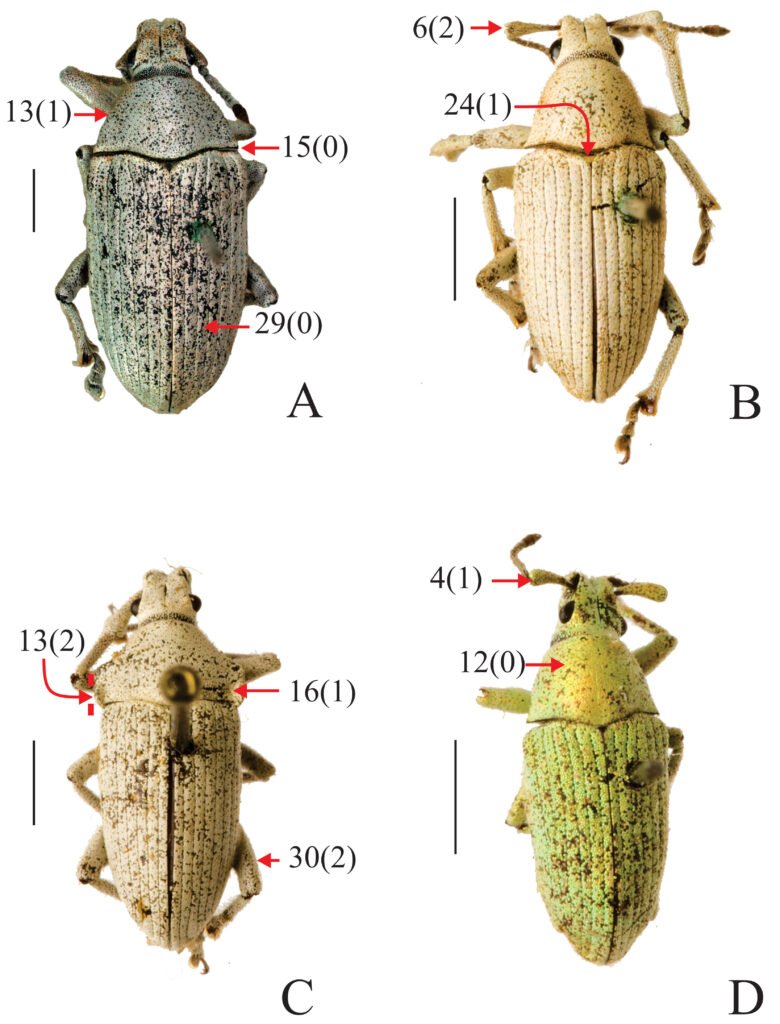
Figure 1. Habitus photographs of Megalostylus species, dorsal view. A) Megalostylus albicans, female; B) M. brevipilis, male; C) M. dilaticollis, male; D) M. fusiformis male. Arrows and numbers indicate character codification, and the character state is indicated between parentheses. Scale bars = 2 mm.
A data matrix of 21 terminal groups and 37 morphological characters was compiled (Table 3). Character states that could not be examined (due to insufficient material) were scored with a “?” and character states with inapplicable entries on various terminals were scored with a “–”. Species or varieties showing 2 or more characters were coded as polymorphic characters. To facilitate the coding, Mesquite software version 3.70 was used (Maddison & Maddison, 2021). An implicit enumeration search was performed in the program TNT version 1.5 (Goloboff & Catalano, 2016). The characters were treated as unordered or non-additive, and under equal weights. The species Pantomorus albosignatus was used to root the trees. To evaluate branch support (BS), a standard Bootstrap with 1000 replicates was calculated in TNT. Branch support values greater than 50 were mapped in the cladogram. The resulting cladogram and character state transformations were examined in WINCLADA under fast optimization. All records were georeferenced, and maps created in ArcMap version 10. 4.1 (ESRI, 2015).
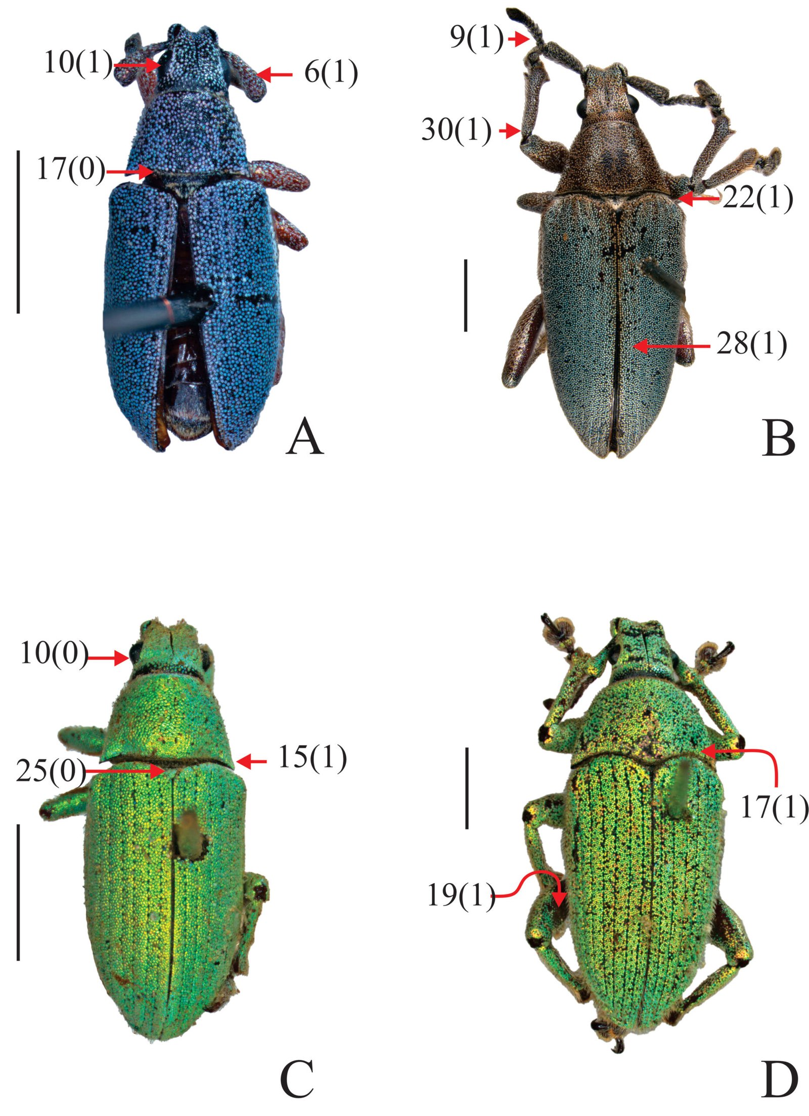
Figure 2. Habitus photographs of Megalostylus species, dorsal view. A) Megalostylus macrophthalmus, male; B) M. rhodopus, male; C) M. splendidus, male; D) M. sturmi, male. Arrows and numbers indicate character codification, the character state is indicated between parentheses. Scale bars = 2 mm.
Results
The search for the most parsimonious trees under equal weights yielded one most parsimonious tree (Fig. 6) (L = 63, IC = 0.73, IR = 0.83), showing the following phylogenetic sequence: (Pantomorus albosignatus (Naupactus cervinus (Megalostylodes hirsutus (Megalostylus)))).
Megalostylodes was found to be sister to the genus Megalostylus based on 12 synapomorphies: epistome scales similar in size, density, and color to those on the rest of the rostrum (0:0), dorsal surface of rostrum slightly to strongly depressed (1:1), absence of pair of dorsolateral carinae (2:0), scape very wide in males and thin in females (3:1), width of scape at apex greater than club width in males (4:1), shape of scape strongly clavate (5:1), color brown to black of the verticillate setae of funicle (9:1), slight lateral projection of pronotum (14:1), absence of a row of denticles on inner margin of protibia (20:0), vestiture of scutellum present, consisting of white scales or seta-like scales (25:1), presence of medial longitudinal depression of ventrites 1 and 2 on males (32:1), and subspherical body shape of spermatheca (33:1). There are also 2 homoplastic characters that support this relationship: pronotum subconical, with sides curved and strongly divergent from apex to base (11:1) and width of base of scutellum wider than interestria 2 (24:2).
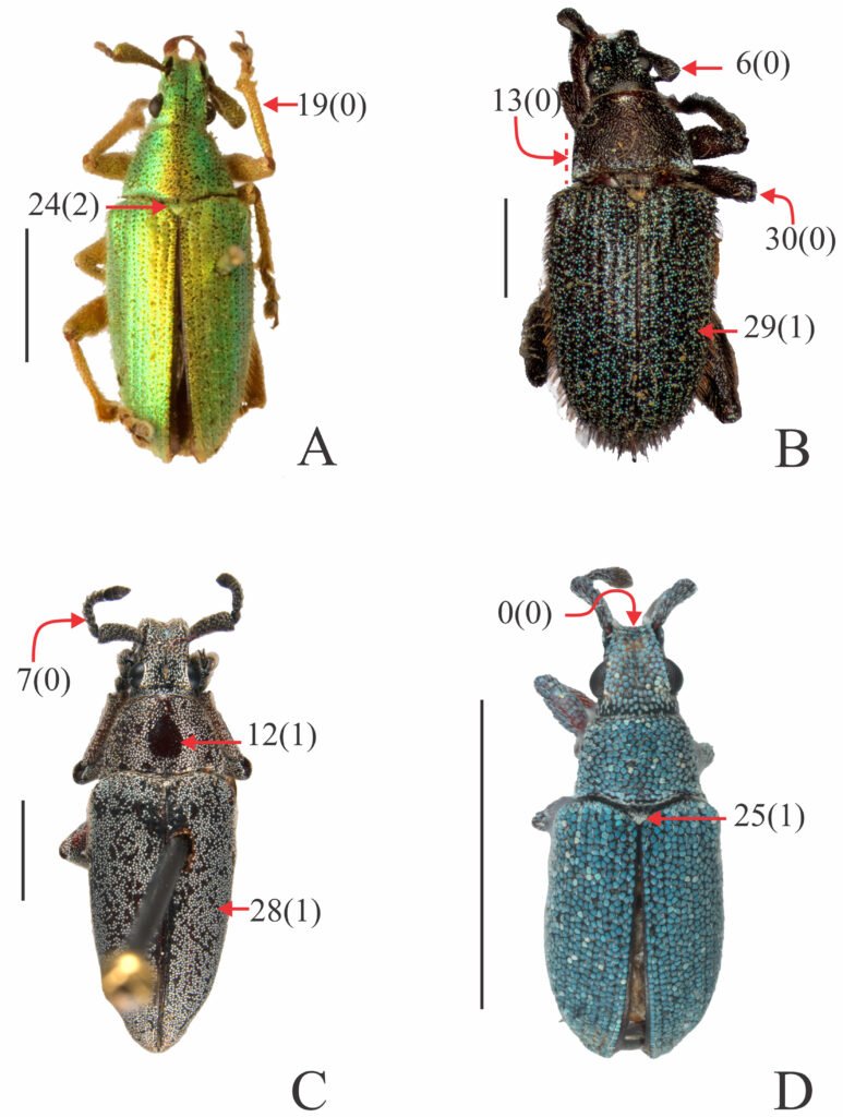
Figure 3. Habitus photographs of Megalostylus species, dorsal view. A) Megalostylus tomentosus, male; B) Megalostylodes hirsutus, male; C) morphospecies 1, male; D) morphospecies 2, male. Arrows and numbers indicate character codification, the character state is indicated between parentheses. Scale bars = 2 mm.
Megalostylus was recovered as monophyletic based on 4 synapomorphies: presence of prominence opposite to mucro in protibia (21:1), elytra in lateral view almost flat (23:1), plate of sternite VIII, subrhomboidal very elongated (34:0), and sculpture of aedeagus smooth (35:1).
The sister genus Megalostylodes is characterized by 3 autapomorphies: pronotum narrower with respect to elytral base (13:0), very long elytral setae, longer than width of elytral interstriae 2 at middle (27:2), and presence of deeply excavated metafemur near apex (31:1), and 3 non-exclusive synapomorphies: presence of glabrous areas in midline of pronotum (12:1), erect disposition of elytral setae (26:1), and slightly convex interestriae (29:1).
Table 1
List of species included in the cladistic analysis of the genus Megalostylus and their geographic distributions (countries and states).
| Species names | Geographic distributions |
| Pantomorus albosignatus Boheman | Mexico (Aguascalientes, Chihuahua, Coahuila, Mexico City, Durango, Guanajuato, Guerrero, Hidalgo, Monterrey, Oaxaca, Puebla Querétaro, San Luis Potosí, Veracruz, Zacatecas) |
| Naupactus cervinus (Boheman) | Argentina (Buenos Aires, Catamarca, Córdoba, Corrientes, Entre Ríos, Jujuy, Mendoza, Misiones, Salta, Santa Fe, Tucumán), Brasil (Paraná, Río Grande do Sul, Santa Catarina, São Paulo), México (Distrito federal), Uruguay (Artigas, Canelones, Colina, Durazno, Maldonado, Montevideo, Rio Negro, Treinta y Tres) |
| Megalostylodes hirsutus Champion | Mexico (Oaxaca) |
| Megalostylus albicans (Lacordaire) | Mexico (Colima, Estado de México, Guanajuato, Guerrero, Jalisco, Michoacán, Morelos, Nayarit, Oaxaca, Puebla) |
| Megalostylus brevipilis Champion | Mexico (Colima, Guerrero, Oaxaca) |
| Megalostylus dilaticollis Champion | Mexico (Guerrero, Michoacán, Morelos, Jalisco) |
| Megalostylus fusiformis Champion | Mexico (Morelos, Guerrero) |
| Megalostylus macrophthalmus Champion | Mexico (Oaxaca) |
| Megalostylus rhodopus Boheman | Mexico (Oaxaca) |
| Megalostylus splendidus Chevrolat | Mexico (Durango, Guerrero, Morelos, Puebla) |
| Megalostylus sturmi Boheman | Mexico (Guerrero, Michoacán) |
| Megalostylus tomentosus Champion | Mexico (Oaxaca) |
Table 2
List of 37 morphological characters, character states and codes.
| Character | Character states |
| 0. Shape, size, density and color of epistome scales compared to those on the rest of the rostrum | Similar in size, density and color (0); smaller, scarcer and generally different in color (1) |
| 1. Dorsal surface of rostrum | Flat (0); slightly to strongly depressed (1) |
| 2. Pair of dorsolateral carinae | Absent (0); present (1) |
| 3. Sexual dimorphism in antennae | Scape width subequal in males and females (0); scape very wide in males and thin in females (1) |
| 4. Width of scape at apex with respect to width of club, in males | Less than club width (0); greater than club width (1) |
| 5. Shape of scape | Capitate (0); strongly clavate (1) |
| 6. Vestiture of scape | Absent to almost absent (0); scales dispersed leaving integument exposed (1); dense, space between scales reduced or absent, not leaving integument exposed (2) |
| 7. Length of funicular antennomeres 1 and 2 | Antennomere 2 slightly shorter than 1 or both sub-equal (0); antennomere 2 longer than 1 (1) |
| 8. Antennae, scales on funicular antennomere 2 | Absent (0); present (1) |
| 9. Color of verticillate setae of funicle | Whitish or golden (0); brown to black (1) |
| 10. Convexity of eyes | Convex, pronounced curvature, hemispherical shape (0); slightly convex, less pronounced curvature, small elevations (1) |
| Table 2. Continued | |
| 11. Shape of pronotum | Subcylindrical, curved sides and maximum width about half (0); subconical, with sides moderately to strongly curved and strongly divergent from apex to base (1); subconical, with sides slightly curved to straight and strongly divergent from apex to base (2); bell-shaped (3); subtrapezoidal, with sides slightly concave at anterior half and progressively expanding towards lateral sides at posterior half (4) |
| 12. Glabrous areas at midline of pronotum | Absent (0); present (1) |
| 13. Width of pronotum with respect to elytral base | Narrower (0); subequal (1); wider (2) |
| 14. Lateral projection of pronotum | Absent or indistinct (0); slightly projected (1); strongly projected (2) |
| 15. Shape of lateral projections of posterior margin of pronotum | Extended towards sides (0); strongly extended backwards, towards elytral base (1) |
| 16. Sides at basal third of pronotum | Not depressed (0); strongly depressed (1) |
| 17. Shape of posterior margin of pronotum | Straight to slightly bisinuate (0); strongly bisinuate (1) |
| 18. Bulging surface beneath intercoxal granule, at anterior margin of prothorax | Indistinct or absent (0); present (1) |
| 19. Color of legs integument | Light tones, reddish or orange (0); dark tones, black or brown (1) |
| 20. Row of denticles on inner margin of protibia | Absent (0); present (1) |
| 21. Prominence opposite to mucro in protibia | Absent (0); present (1) |
| 22. Elytral anterior margin | Straight (0); bisinuate (1) |
| 23. Shape of elytra in lateral view | Moderately convex (0); almost flat (1) |
| 24. Width of base of scutellum with respect to width of interstria 2 | Reduced to indistinct (0); subequal to width of interstria 2 (1); wider than interstria 2 (2) |
| 25. Scutellum vestiture | Scales similar in color to those covering whole surface of elytra (0); Scales similar, consisted of white scales or seta-like scales (1) |
| 26. Disposition of elytral setae | Recumbent to suberect (0); erect (1) |
| 27. Size of elytral setae | Short (0); long, almost as long as width of interstria 2 at middle (1); very long, longer than width of elytral interestriae 2 at middle (2) |
| 28. Arrangement of elytral setae | Uniform throughout elytral disc (0); only on lateral edges of elytral disc, dorsally without setae (1) |
| 29. Convexity of interstriae | Flat (0); slightly convex (1) |
| 30. Vestiture on legs | Absent or almost absent (0); inconspicuous, scales are scattered leaving integument exposed (1); conspicuous, space between scales is reduced or absent, and covered the integument (2) |
| 31. Deep excavation on metafemur, near apex | Absent (0); present (1) |
| 32. Medial longitudinal depression of ventrites 1 and 2, on males | Indistinct or absent (0); present (1) |
| 33. Spermatheca, body shape | Subcylindrical, slender (almost as wide as base of cornu) (0); subspherical (1) |
| 34. Shape of plate of sternite VIII | Subrhomboidal very elongated, with basal part much longer than apical part (0); subrhomboidal slightly elongated, with basal part as long as apical part (1) |
| 35. Aedeagus, sculpture of median lobe | Granulose (0); smooth (1) |
| 36. Aedeagus, shape of apex of median lobe | Acute to slightly acute (0); truncated (1); arrow shape (2) |
Table 3
Data matrix of 21 taxa and 37 morphological characters of Megalostylus and outgroups used for the cladistic analysis. Inapplicable characters are indicated with a dash (-), and missing characters with a question mark (?).
| Taxa | Characters | ||||||
| 0-4 | 5-9 | 10-14 | 15-19 | 20-24 | 25-29 | 30-36 | |
| Pantomorus albosignatus | 101?0 | 00000 | 00010 | 00000 | 10000 | -0100 | 00?01?? |
| Naupactus cervinus | 10100 | 00100 | 00010 | 00000 | 10100 | 00000 | 00001?2 |
| Megalostylodes hirsutus | 01011 | 10001 | 01101 | 00000 | 00102 | 11201 | 0111100 |
| Megalostylus albicans | 01011 | 12010 | 02012 | 00101 | 01111 | 00000 | 1011010 |
| Megalostylus albicans var. expansus | 01011 | 12010 | 02022 | 00101 | 01111 | 00000 | 101??10 |
| Megalostylus albicans var. farinosus | 01011 | 120?0 | 02012 | 00101 | 01111 | 00000 | 101???? |
| Megalostylus brevipilis | 010?1 | 120?0 | 03011 | 10101 | 01111 | 00000 | 101??10 |
| Megalostylus dilaticollis | 01011 | 12000 | 04022 | 01001 | 01111 | 00000 | 10110?? |
| Megalostylus fusiformis | 010?1 | 120?0 | 03011 | 10101 | 01111 | 00000 | 10????? |
| Megalostylus macrophthalmus | 01011 | 100? | 12011 | 00000 | 01112 | 10000 | 00?10?? |
| Megalostylus splendidus | 01011 | 12010 | 01011 | 10101 | 01112 | 00000 | 1011010 |
| Megalostylus splendidus var. | 01011 | 12010 | 01011 | 10101 | 01112 | 00000 | 1011010 |
| Megalostylus sturmi | 01011 | 12010 | 0100&11 | 10111 | 01112 | 01100 | 1011?11 |
| Megalostylus sturmi var. villosus | 01011 | 12010 | 0100&11 | 10111 | 01112 | 01100 | 1011011 |
| Megalostylus rhodopus | 01011 | 12001 | 01111 | 00000 | 01112 | 10010 | 0011010 |
| Megalostylus tomentosus | 01011 | 110?0 | 02011 | 00000 | 01112 | 01100 | 00110?? |
| Morphospecies 1 | 010?1 | 12001 | 01111 | 10000 | 0111? | 10010 | 001??10 |
| Morphospecies 2 | 010?1 | 11000 | 01011 | 10100 | 01112 | 10000 | 001??10 |
| Morphospecies 3 | 010?1 | 10001 | 02011 | 00000 | 01112 | 10011 | 001??10 |
| Morphospecies 4 | 010?? | 11000 | 02011 | 00000 | 01112 | 01100 | 00?10?? |
| Morphospecies 5 | 010?1 | 12000 | 04011 | 00001 | 01111 | 00000 | 101??10 |
Two main clades were found within Megalostylus: clade I, including Megalostylus rhodopus and morphospecies 1 and 3 (considered belonging to M. rhodopus), is supported by 1 exclusive synapomorphy: elytral setae only present on the lateral edges of elytral disc (28:1). Clade II is supported by 1 exclusive synapomorphy and 1 non-exclusive synapomorphy: scales of scape separate, leaving integument exposed (6:1) and whitish or golden color of the verticillate setae of funicle (9:0), respectively. Within clade II, morphospecies2 is sister to the remaining species, which form a clade supported by 1 non-exclusive synapomorphy: pronotum subconical, sides slightly curved to straight and strongly divergent from apex to base (11:2). Megalostylus macrophthalmus is the sister species of M. tomentosus–M. sturmi var. villosus based on 1 non-exclusive synapomorphy: vestiture of scutellum present, scales similar in color to those covering the whole surface of elytra (25:0). Megalostylus tomentosus (along with morphospecies4) is the sister of a supported clade (BT 58) M. dilaticollis–M. sturmi var. villosus clade, which is supported by 3 exclusive synapomorphies and 1 non-exclusive synapomorphy: integument of legs with dark tones, black or brown (19:1), and width of base of scutellum reduced to indistinct (24:1), vestiture on legs inconspicuous, scales are scattered leaving integument exposed (30:1), and scales separated leaving integument of scape exposed (6:2). Within this clade M. dilaticollis (along with morphospecies 5) is sister to a subclade supported by 1 exclusive synapomorphy and 1 non-exclusive synapomorphy: presence of scales on the second funicular antennomere (8:1) and posterior margin of pronotum strongly bisinuate (17:1) that includes M. albicans and its varieties, M. albicans var. expansus, and var. farinosus sister to M. brevipilis to M. sturmi var. villosus clade supported by 1 exclusive synapomorphy and 1 non-exclusive synapomorphy: pronotum flared or bell-shaped (11:3) and lateral projections of posterior margin of pronotum strongly extended backward, towards elytral base (15:1). Within this clade, M. brevipilis and M. fusiformis are sisters to the M. splendidus–M. sturmi var. villosus clade which is supported by 2 non-exclusive synapomorphies: pronotum subconical, sides curved and strongly divergent from apex to base (11:1), and width of base of scutellum wider than interestria 2 (24:2). The clade M. splendidus–M. sturmi var. villosus also has unresolved relationships between M. splendidus and his variety, both sister to the M. sturmi + M. sturmi var. villosus clade.
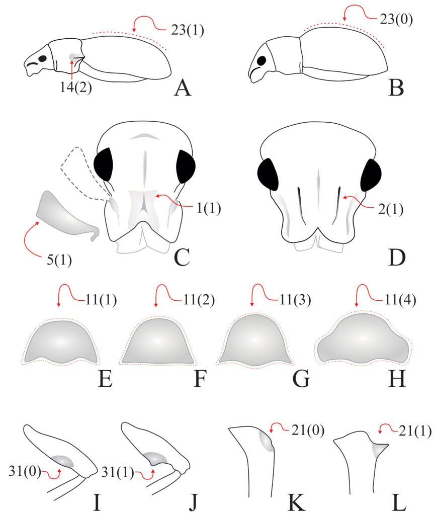
Figure 4. Diagrammatic illustrations with arrows and numbers indicating character codification of head, pronotum, legs, and elytra in Megalostylus and outgroup species. A) Megalostylus dilaticollis, lateral view; B) Pantomorus albosignatus, lateral view; C) M. rhodopus, head; D) Naupactus cervinus, head; E) M. sturmi, pronotum; F) M. tomentosus, pronotum; G) M. brevipilis, pronotum; H) M. dilaticollis, pronotum; I) M. albicans, metafemora; J) Megalostylodes hirsutus, metafemora; K) M. hirsutus, protibiae; L) M. albicans, protibiae.
Geographic distribution. The maps (Figs. 7, 8) indicate that the species of Megalostylus are mostly distributed along the Pacific coast, with the greatest richness in the central and southern parts of the country. Megalostylus albicans shows the largest distribution,ranging from Oaxaca to Sinaloa. Six species are distributed in the central states of the country (Guanajuato, Guerrero, Michoacán, Morelos, and Puebla): M. albicans, M. brevipilis, M. dilaticollis, M. fusiformis, M. splendidus, and M. sturmi. The species M. rhodopus, M. macrophthalmus, and M. tomentosus are restricted to Oaxaca, and M. rhodopus reaches the southernmost distribution extending to the Isthmus of Tehuantepec.
Discussion
The sister group relationship between Megalostylodes and Megalostylus is well supported by 12 exclusive synapomorphies, and the monophyly of Megalostylus is supported by a combination of 4 exclusive synapomorphies of the protibiae, elytra, and female and male genitalia. Champion (1911) distinguished Megalostylus based on the presence of a prominence opposite to mucro (or toothed tibiae at the external apical angle), and Lanteri and del Río (2017) recovered this character state (car 69[1]) as an apomorphy of Megalostylus.
Within Megalostylus most of the relationships are not well supported nevertheless, it is clear the position of M. rhodopus (including morphospecies 1 and 3) as sister species of the remaining, and it was recovered a well-supported group including M. dilaticollis (= morphospecies 5), M. albicans, M. brevipilis, M. fusiformis, M. splendidus, and M. sturmi. Megalostylus macrophthalmus and M. tomentosus (= morphospecies 4) would be basal regarding this clade. Morphospecies2 is considered a probable new species, however, this status needs further studies.
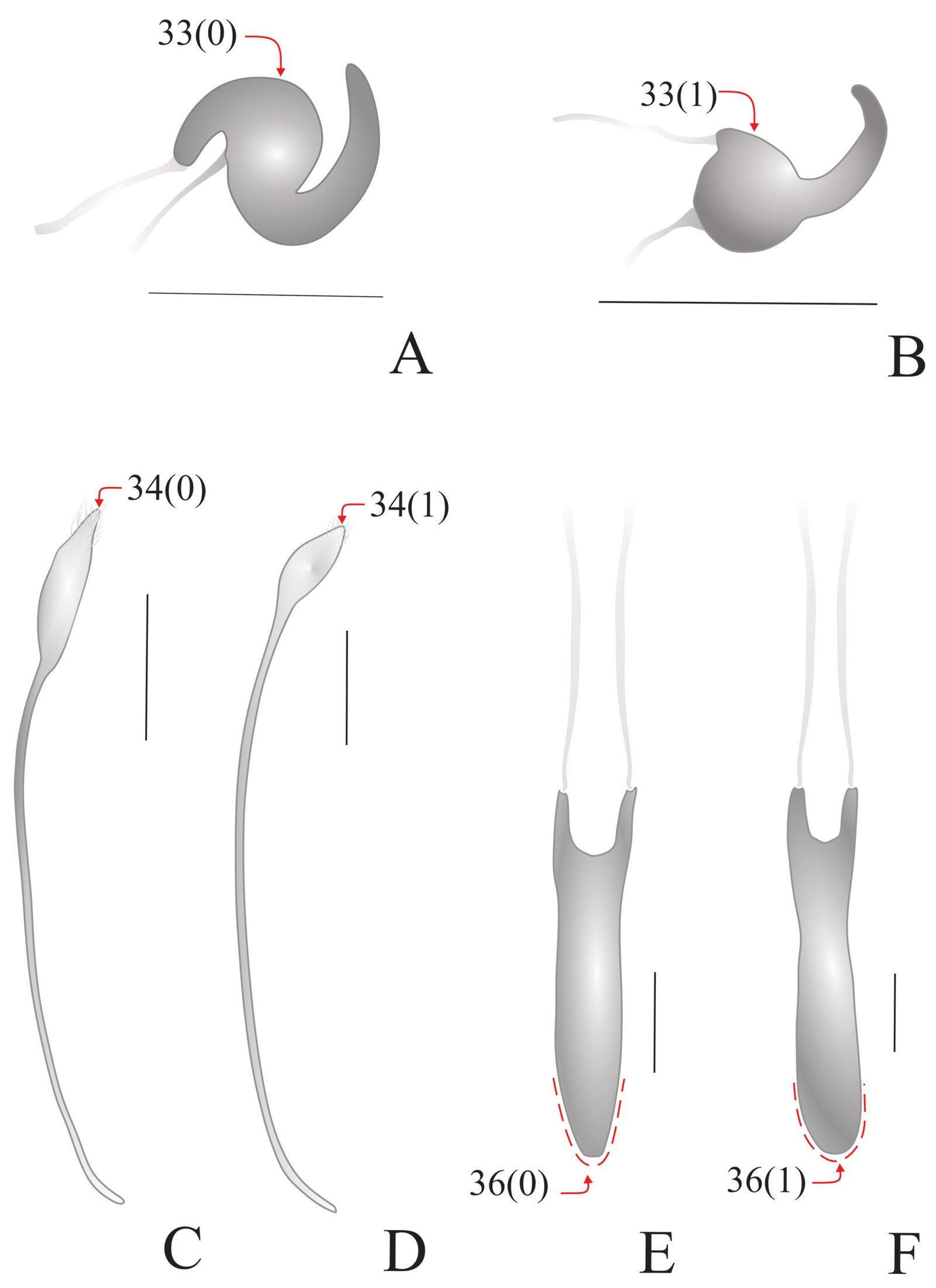
Figure 5. Diagrammatic illustrations with arrows and numbers indicating character codification of female and male genitalia in Megalostylus and outgroup species. A) Pantomorus albosignatus, spermatheca; B) M. albicans, spermatheca; C) M. splendidus, sternite VIII; D) Megalostylodes hirsutus, sternite VIII; E) M. rhodopus, aedeagus; F) M. sturmi, aedeagus. Scale bars = 0.5 mm.
The species of Megalostylus are very variable in scale color, size and pronotum shape, and due to that intraspecific variation, some nominal species have been synonymized: M. farinosus Chevrolat, 1878 [junior synonym of M. albicans (Lacordaire, 1876)], M. expansus Pascoe, 1881 [junior synonym of M. albicans (Lacordaire, 1876)] and M. villosus Chevrolat, 1878 [junior synonym of M. sturmi Boheman, 1840]. Our analysis explored the relationships among intraspecific varieties of the genus Megalostylus, and the results support the previously established synonymies. In the case of M. albicans with its varieties (M. albicans var. expansus and M. albicans var. farinosus) there is no reason to consider them as different species. Characters with the greatest contribution to the species relationships are those referring mainly to the vestiture of antennae, legs, elytra, shape, and characteristics of the pronotum, scutellum, and apex of aedeagus.
Figure 6. Most parsimonious cladogram of Megalostylus plus 3 outgroups under equal weights, showing character fast optimization. Black circles indicate synapomorphies, whereas white circles indicate non-exclusive synapomorphies. Numbers on and below each circle correspond to character and state codes, respectively. Bootstrap values are indicated below the branches.
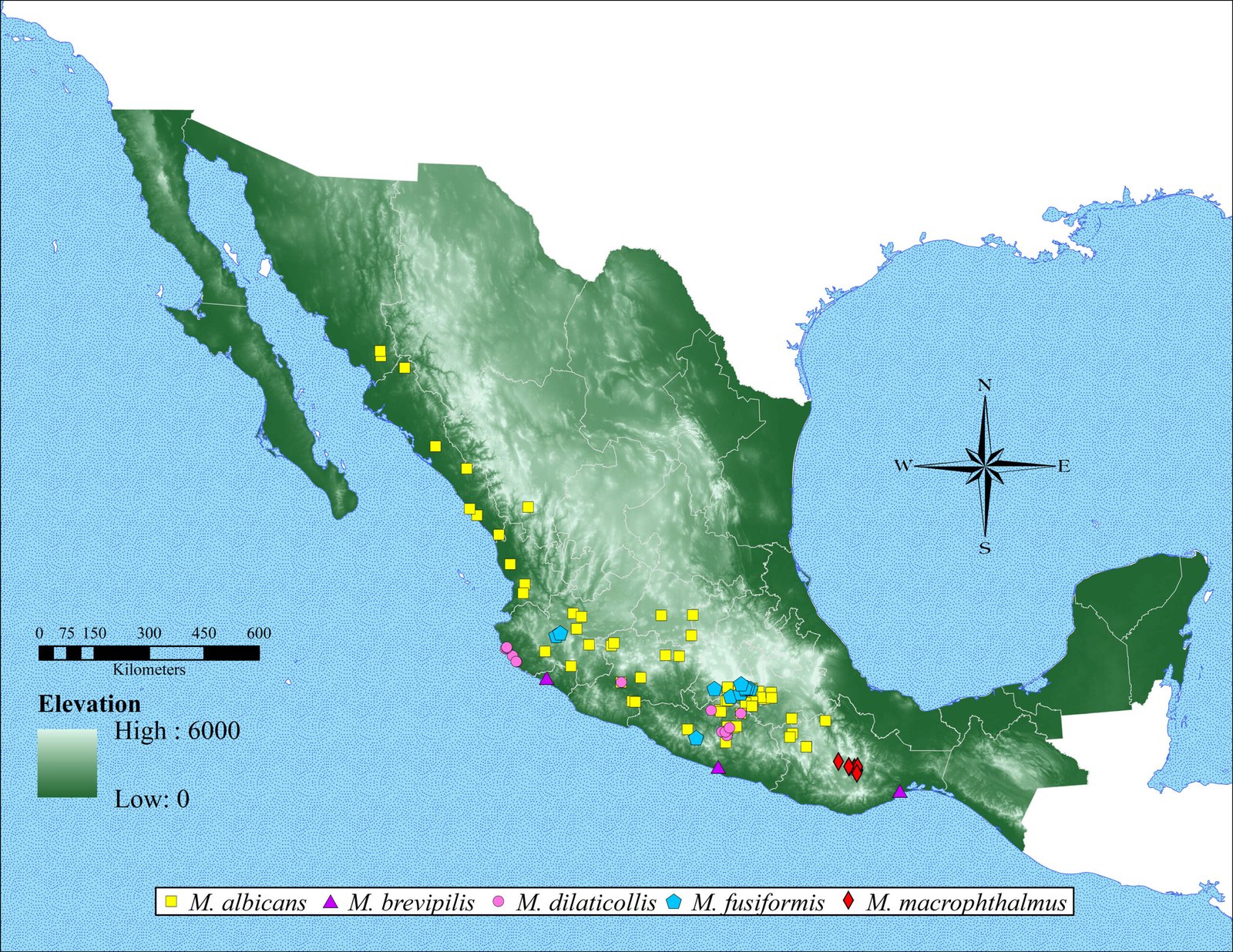
Figure 7. Occurrence map of 5 Megalostylus species, ordered alphabetically. Megalostylus albicans (yellow square); M. brevipilis (purple triangle); M. dilaticollis (pink circle); M. fusiformis (blue pentagon) and M. macrophthalmus (red diamond). Map by A. Lizama-Hernández.
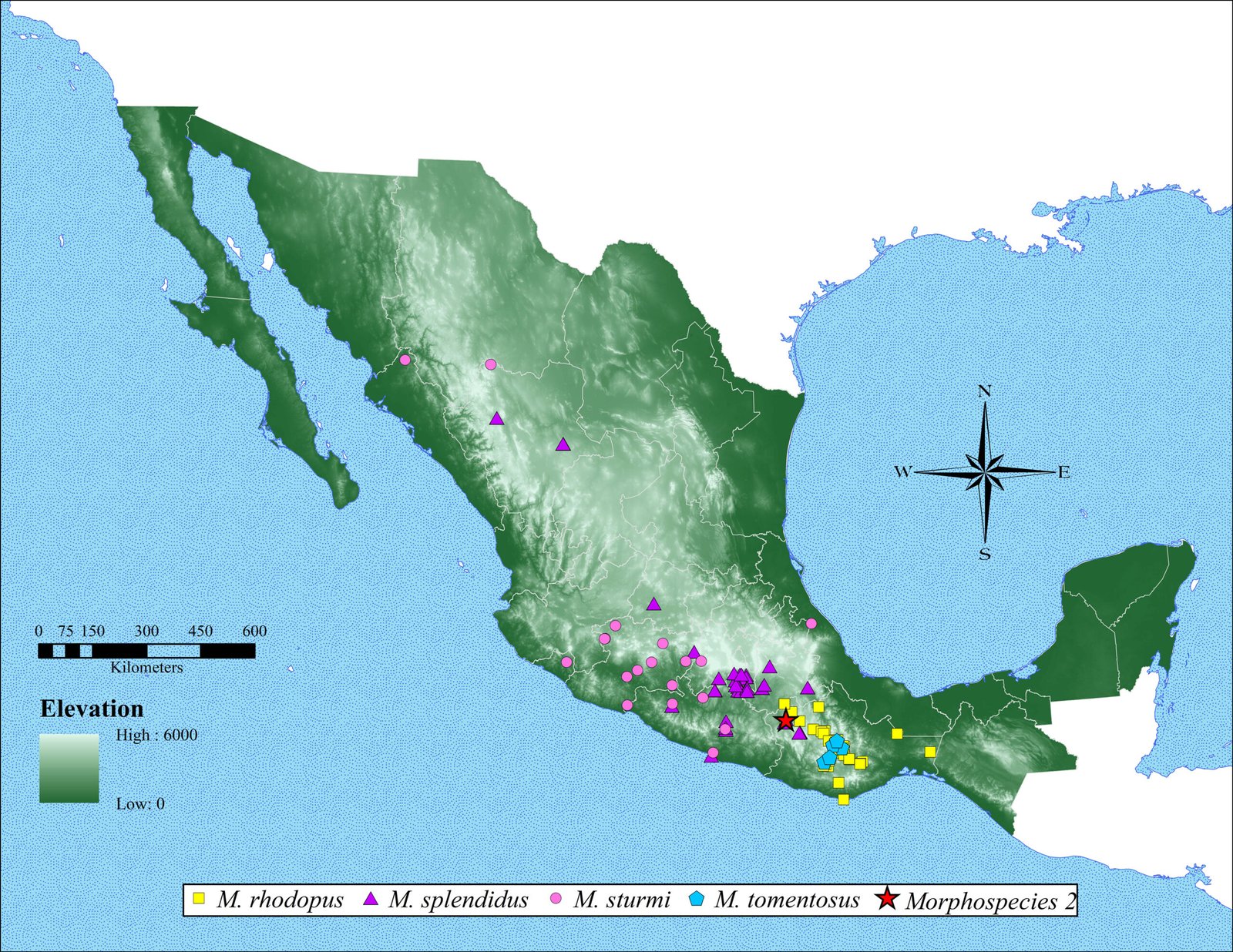
Figure 8. Occurrence map of remaining 4 Megalostylus species, ordered alphabetically plus a new Megalostylus species (indicated here as morphospecies 2). Megalostylus rhodopus (yellow square); M. splendidus (purple triangle); M. sturmi (pink circle); M. tomentosus (blue pentagon) and morphospecies 2 sp. nov. (red star). Map by A. Lizama-Hernández.
Acknowledgments
We thank all curators, institutions, collection managers, technicians, and collectors that provided specimens. We also thank Miguel Menéndez-Acuña, Elizabeth Arellano-Arenas, and anonymous reviewers for their helpful suggestions to improve the manuscript. The authors would like to express their sincerest gratitude to Santiago Zaragoza Caballero and María Cristina Mayorga Martínez for their invaluable assistance in providing material for examination.
References
Champion, G. C. (1911). Insecta. Coleoptera. Vol. IV, Parte 3. Rhynchophora. Curculionidae. Attelabinae, Pterocolinae, Allocoryninae, Apioninae, Thecesterninae, Otiorhynchinae. In D. Sharp, & G. Champion (Comps.), Biologia Centrali-Americana (pp. 241–246). London: R.H. Porter.
del Río, M. G. (2009). Estudio taxonómico y cladístico de los géneros de la tribu Naupactini (Coleoptera: Curculionidae) distribuidos en la subregión Páramo-Puneña o Zona de Transición Sudamericana (Ph.D. Thesis). Universidad Nacional de la Plata, La Plata, Argentina.
ESRI (2015). ArcGIS Desktop: Versión 10.4.1 Redlands, CA: Environmental Systems Research Institute.
Goloboff, P. A., & Catalano, S. A. (2016). TNT version 1.5, including a full implementation of phylogenetic morphometrics. Cladistics, 32, 221–238. https://dx.doi.org/10.1111/cla.12160
Lanteri, A. A., & del Río, M. G. (2017). Phylogeny of the tribe Naupactini (Coleoptera: Curculionidae) based on morphological characters. Systematic Entomology, 42, 429–447. https://doi.org/10.1111/syen.12223
Maddison, W. P., & Maddison, D. R. (2021). Mesquite: a modular system for evolutionary analysis. Versión 3.70. http://www.mesquiteproject.org
Muñiz-Vélez, R., Burgos-Dueñas, A., Burgos-Dueñas, O., López-Martínez, V., & Burgos-Solorio, A. (2015). Nuevas aportaciones a los Curculionoidea del estado de Morelos, Folia Entomológica Mexicana, 1, 25–49.
Ordóñez-Reséndiz, M. M., Muñíz-Vélez R., & Gama-Rojas, F. (2008). Curculiónidos (Coleópteros). In S. Oceguera, & J. Llorente-Bousquets (Coords.), Catálogo taxonómico de especies de México, en Capital natural de México, vol. L. Conocimiento actual de la biodiversidad. CD1. Mexico City. Conabio.
Rosas, M. V., Morrone, J. J., del Río, M. G., & Lanteri, A. A. (2011). Phylogenetic analysis of the Pantomorus-Naupactus complex (Coleoptera: Curculionidae: Entiminae) from North and Central America. Zootaxa, 2780, 1–19. https://doi.org/10.11646/zootaxa.2780.1.1
Schoenherr, C. J. (Ed). (1840). Genera et species curculionidum, cum synonymia hujus familiae; species novae aut hactenus minus cognitae. Paris: Roret.

Riqueza fitoplanctónica y nuevos registros de dinoflagelados, diatomeas, cocolitofóridos y bigiros, en aguas oceánicas del Caribe colombiano
Karen Ayala-Galván a, *, José Manuel Gutiérrez-Salcedo a y Jose Ernesto Mancera-Pineda b
a Instituto de Investigaciones Marinas y Costeras “José Benito Vives de Andréis”, Grupo de Investigación en Taxonomía, Sistemática y Ecología Marina, Calle 25 Núm. 2-55, Playa Salguero, Santa Marta D.T.C.H., Magdalena, Colombia
b Universidad Nacional de Colombia, Grupo de Investigación en Modelación de Ecosistemas Costeros, Carrera 45 Núm. 26-85, Ciudad Universitaria, Teusaquillo, Bogotá D.C., Colombia
*Autor para correspondencia: ayalakarenc08@gmail.com (K. Ayala-Galván)
Resumen
Para las aguas oceánicas del Caribe colombiano existe un número limitado de publicaciones sobre la composición específica del fitoplancton, la mayoría es literatura gris. Hasta la fecha, se reportan para el Caribe colombiano 328 especies de diatomeas y 185 especies de dinoflagelados, que son principalmente registros en aguas neríticas. Con el fin de ampliar el conocimiento de la riqueza y aumentar el listado taxonómico existente en aguas oceánicas, se analizó la composición fitoplanctónica en la provincia oceánica del Caribe central colombiano, en un área estratégica que comprende 35,874 km2, representa 7.5% de las aguas oceánicas y se ubica frente a la influencia del río Magdalena. Para esto, se recolectaron 108 muestras entre 2015 y 2017 con botellas Niskin a 10, 80 y 250 m, y arrastres verticales con redes de 20 µm de poro de malla en los primeros 50 m. Se identificaron 287 taxones pertenecientes a dinoflagelados, diatomeas, cianobacterias, clorofitas, silicoflagelados, cocolitofóridos, criptofitas, carofitas y bigiros, encontrando mayor riqueza de dinoflagelados (61.32%) y diatomeas (30.64%). El listado taxonómico comprende 184 especies, 74 nuevos registros para la cuenca del Caribe colombiano; se incrementa la composición específica para dinoflagelados en 27.03% y para diatomeas en 2.44%.
Palabras clave: Comunidad fitoplanctónica; Mesoescala; Zona oceánica; Listado taxonómico
Phytoplanktonic richness and new records of dinoflagellates, diatoms, coccolithophorids and bigyrids in oceanic waters of the Colombian Caribbean
Abstract
For the oceanic waters of the Colombian Caribbean there is a limited number of publications on the specific composition of phytoplankton, most of which are in gray literature. To date, 328 species of diatoms and 185 species of dinoflagellates have been reported for the Colombian Caribbean, mainly from neritic waters. In order to expand the knowledge of the richness and increase the existing taxonomic list in oceanic waters, the phytoplankton composition was analyzed in the oceanic province of the central Colombian Caribbean, in a strategic area that comprises 35,874 km2, represents 7.5% of the oceanic waters and is located in front of the influence of the Magdalena River. For this, 108 samples were collected between 2015 and 2017 with Niskin bottles at 10, 80 and 250 m, and vertical trawls with 20 µm mesh pore nets in the first 50 m. A total of 287 taxa belonging to dinoflagellates, diatoms, cyanobacteria, chlorophytes, silicoflagellates, coccolithophorids, cryptophytes, carophytes and bygira were identified, finding greater richness of dinoflagellates (61.32%), and diatoms (30.64%). The taxonomic list includes 184 species, with 74 new records reported for the Colombian Caribbean basin, increasing the specific composition for dinoflagellates by 27.03% and for diatoms by 2.44%.
Keywords: Phytoplankton community; Mesoscale; Oceanic zone; Taxonomic listing
Introducción
El fitoplancton se ha estudiado a lo largo de la historia en diferentes lugares del mundo y se reconoce como el principal productor primario de los ambientes marinos. Sin embargo, su análisis es un reto debido a que es una comunidad dinámica y su composición, densidad y distribución pueden variar drásticamente con el tiempo, desde variabilidad decenal (Henson et al., 2009), interanual (Westberry et al., 2016), estacional (Holligan y Harbour, 1977), y hasta ciclos de marea (Davidson et al., 2013). A pesar de ser objetivo de muchas investigaciones, su conocimiento en las provincias neríticas y oceánicas de diferentes latitudes es muy irregular, lo que no es ajeno al mar Caribe colombiano.
Ubicado en la parte más interna de la cuenca semicerrada del Caribe, el mar Caribe colombiano posee aguas de gran extensión, con 30,219 km2 de aguas costeras y 501,935 km2 de aguas oceánicas (INVEMAR, 2015). Estas últimas tienen un sistema complejo y se ven afectadas en la parte central por una convergencia de procesos como el clima, corrientes y giros marinos, eventos de surgencia, y un dominio costero que incide en las descargas continentales principalmente del río Magdalena, que dan lugar a la modificación de los reguladores ambientales y a la disposición de recursos, los cuales son determinantes en la composición, estructura y biomasa fitoplanctónica (Álvarez-León et al., 1995; Andrade y Barton, 2005; Bernal et al., 2006; Ricaurte-Villota y Bastidas-Salamanca, 2017).
La gran extensión de aguas oceánicas y los diferentes procesos que influyen en ellas dificultan operacionalmente los muestreos y aumentan los costos de estudio, éste es uno de los motivos por los cuales los análisis de fitoplancton marino se encuentran seccionados en diferentes áreas y se encuentran enfocados, principalmente, a una escala local (> 1 km) (Ávila-Silva, 2018; Ayala-Galván et al., 2017, 2018, 2021; Campos-González, 2007; Garay et al., 1988; Garrido-Linares, Alonso-Carvajal, Gutiérrez-Salcedo et al., 2014; Garrido-Linares, Alonso-Carvajal, Rueda et al., 2014; INVEMAR et al., 2017; INVEMAR-ANH, 2012; Ricaurte-Villota et al., 2018; Téllez et al., 1988; Vides y Alonso, 2016); con excepción de algunos análisis que se han realizado a gran escala (> 1,000 km) como los de INVEMAR-ANH (2008), INVEMAR-ANH (2010), Lozano-Duque et al. (2010a), Salón (2013) y Ayala-Galván y Gutiérrez-Salcedo (2019). Aunque los objetivos de estos estudios incluyen caracterizaciones, descripción de los atributos ecológicos e identificación de patrones espaciales o temporales, la información se encuentra restringida debido a que la mayoría de trabajos se encuentran en literatura gris, con algunas excepciones (Ayala-Galván et al., 2022; Garay et al., 1988; Lozano-Duque et al., 2010a). En este contexto, se ha identificado que la mayoría de trabajos del fitoplancton marino en aguas oceánicas provienen de estudios técnicos entre la alianza institucional entre el Instituto de Investigaciones Marinas y Costeras (INVEMAR) y la Agencia Nacional de Hidrocarburos (ANH) de Colombia, por lo que se espera dar mayor visibilidad a esta información, enfocando el objetivo de este trabajo en conocer la riqueza del fitoplancton marino en aguas oceánicas.
Materiales y métodos
El área de estudio comprende 27 sitios de muestreo que se encuentran ubicados en la provincia oceánica de la región central de la cuenca del Caribe colombiano, sobre el abanico sedimentario del Magdalena (Molina et al., 1994), frente al litoral costero comprendido entre los departamentos de Sucre y Magdalena. Tiene un área total de 35,874 km2 con una distancia mínima de la costa de aproximadamente 20 km y máxima de 296 km y con una profundidad entre 400 y 4,500 m (fig. 1).
Para la recolecta de muestras y datos se realizaron 3 campañas de muestreo en los años 2015, 2016 y 2017, que para los análisis corresponden a sectores (tabla 1). En cada estación se realizó un arrastre vertical con una red cónica de 2.2 m de longitud, con diámetro de boca de 0.58 m y 20 µm de poro de malla (tabla 2). El material biológico recolectado se almacenó en contenedores de plástico de 500 ml y se fijó con formalina neutralizada con bórax (tetraborato de sodio) quedando una solución final concentrada al 4% (Boltovskoy, 1981). Adicionalmente, en cada estación se muestrearon 3 profundidades, de las cuales 2 pertenecen a la zona epipelágica (ep) y corresponden a las masas de agua: agua superficial del Caribe (ASC) y agua subsuperficial subtropical (ASS); y una pertenece a la zona mesopelágica (mp) que corresponde a la masa de agua ASS (tabla 2). Para ésto, se realizó el lance de una roseta oceanográfica equipada con botellas Niskin de 10 L de capacidad, de los cuales se almacenaron 800 ml de agua en contenedores de plástico forrados con vinipel negro (para evitar la penetración de la luz) y se les adicionó 8 ml de lugol ácido en proporción 1:100.
Tabla 1
Coordenadas geográficas de las estaciones de muestreo de la comunidad fitoplanctónica en el Caribe central colombiano. Época climática (Pujos et al., 1986): inicio (+) final (–) foco (*).
| Sector | Época | Estación | Fecha | Coordenadas decimales de la estación | |
| (día-mes-año) | Latitud | Longitud | |||
| Central | Lluvia (–) Seca (+) | 409 | 19/11/2015 | 12.0833330 | -74.12500000 |
| 412 | 21/11/2015 | 12.4166670 | -74.37500000 | ||
| 414 | 22/11/2015 | 12.2500000 | -74.62500000 | ||
| 416 | 24/11/2015 | 12.0833330 | -74.87500000 | ||
| 418 | 25/11/2015 | 12.4166670 | -74.87500000 | ||
| 421 | 29/11/2015 | 11.9166670 | -75.12500000 | ||
| 425 | 01/12/2015 | 12.0833330 | -75.37500000 | ||
| 431 | 02/12/2015 | 11.7500000 | -75.62500000 | ||
| 433 | 12/12/2015 | 11.5833330 | -75.87500000 | ||
| Externo | Seca (–) | 435 | 09/04/2016 | 12.9166670 | -74.12500000 |
| 437 | 10/04/2016 | 12.5833330 | -74.12500000 | ||
| 444 | 12/04/2016 | 12.5833330 | -74.62500000 | ||
| 446 | 14/04/2016 | 12.7500000 | -74.87500000 | ||
| 451 | 15/04/2016 | 12.4211390 | -75.10350000 | ||
| 456 | 17/04/2016 | 12.9166670 | -75.37500000 | ||
| 459 | 18/04/2016 | 12.7500000 | -75.62500000 | ||
| 462 | 19/04/2016 | 12.4166670 | -75.87500000 | ||
| 466 | 20/04/2016 | 12.0833330 | -75.62500000 | ||
| 467 | 21/04/2016 | 12.0833330 | -75.87500000 | ||
| Interno | Lluvia (*) | 555 | 23/09/2017 | 11.3242194 | -74.77517500 |
| 557 | 24/09/2017 | 11.2579280 | -75.31736700 | ||
| 559 | 02/10/2017 | 11.9754720 | -74.05918300 | ||
| 561 | 03/10/2017 | 11.8466639 | -74.39910556 | ||
| 564 | 04/10/2017 | 11.9823806 | -74.99378333 | ||
| 566 | 07/10/2017 | 11.5472722 | -75.18444444 | ||
| 567 | 26/09/2017 | 11.7407390 | -75.39539700 | ||
| 570 | 08/10/2017 | 11.4804944 | -75.83584722 |
Tabla 2
Información asociada a las 108 muestras en el área de estudio.
| Año | Sector | Núm. de estaciones | Análisis | Método | Profundidad (metros) | Núm. de muestras |
| 2015 | Central | 9 | Cualitativo | Red | 20 – 0 m | 9 |
| Cuantitativo | Botella | ASC-ep (10 m) | 27 | |||
| ASS-ep (80 m) | ||||||
| ASS-mp (250 m) | ||||||
| 2016 | Externo | 10 | Cualitativo | Red | 20 – 0 m | 10 |
| Cuantitativo | Botella | ASC-ep (10 m) | 30 | |||
| ASS-ep (80 m) | ||||||
| ASS-mp (250 m) | ||||||
| 2017 | Interno | 8 | Cualitativo | Red | 50 – 0 m | 8 |
| Cuantitativo | Botella | ASC-ep (30m) | 24 | |||
| ASS-ep (80m) | ||||||
| ASS-mp (250m) |
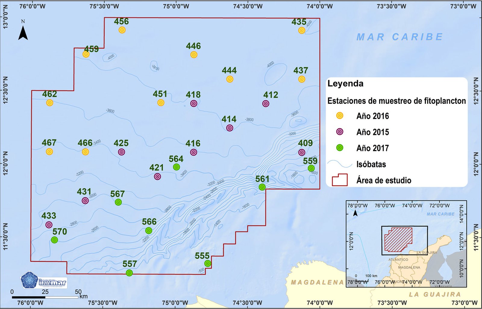
Figura 1. Área de estudio, ubicada en el centro de la cuenca del Caribe colombiano. Fuente: Laboratorio de sistemas de información – LabSIS/ INVEMAR.
Las muestras de red se revisaron por alícuotas (0.125 ml) mediante una gráfica de morfoespecies acumulada (Ramírez, 1999). Las muestras de botella se revisaron con el método Utermöhl, que se encuentra detallado en el manual de fitoplancton de Edler y Elbrächter (2010). Las células se observaron en un microscopio invertido marca Leica Microsystems modelo DMi1, con objetivos de 20X, 40X y 63X, las fotografías se tomaron con una cámara Leica Microsystems MC120 HD y fueron procesadas con el software de adquisición de imágenes LAS EZ. La identificación se realizó por morfología al nivel más bajo posible siguiendo las claves taxonómicas de Cupp (1943), Wood (1963), Taylor (1976), Balech (1988), Round (1990), Tomas (1997), Vidal (2010), Hoppenrath et al. (2009), entre otras. La información taxonómica se tabuló y actualizó siguiendo la nomenclatura de la base de datos mundial de algas AlgaeBase (Guiry y Guiry, 2025). Luego de la identificación y análisis, todas las muestras biológicas se depositaron en la colección de plancton del Museo de Historia Natural Marina de Colombia MAKURIWA.
Con el fin de generar una descripción completa a nivel de composición, se unificaron las matrices de presencia de las muestras con red y de botellas Niskin. Se realizó una descripción general de las categorías taxonómicas encontradas y de la riqueza a nivel horizontal. Así mismo, se describió la riqueza por grupo fitoplanctónico y solo en el caso de los 2 géneros más representativos (Tripos Bory, 1823 y Chaetoceros Ehrenberg, 1844) se detalló la variación horizontal. Además, se mencionan las especies frecuentes y raras para el área de estudio. Finalmente, al inventario se le realizó la verificación de registros nuevos de especies basados en listados previos para el Caribe colombiano.
La riqueza de especies (S) se calculó con el programa Primer V7 (Clarke y Gorley, 2015) y las salidas gráficas con el programa Ocean Data View, a las que se les realizó una interpolación de variación de datos DIVA (Schlitzer, 2022). Para esta última se consideró cada estación como una réplica aleatoria, teniendo en cuenta que, las características conservativas que separan las masas de agua oceánicas del Caribe central colombiano se dan de forma estratificada (Dorado-Roncancio et al., 2022).
Resultados
Mediante los muestreos con redes y botellas Niskin, en el Caribe central colombiano se registraron en total 287 taxones fitoplanctónicos, que se distribuyeron en 90 géneros, 60 familias, 37 órdenes, 13 clases y 8 phyla (Dinoflagellata, Heterokontophyta, Cyanobacteria, Chlorophyta, Haptophyta, Cryptista, Charophyta y Bigyra). El listado taxonómico se encuentra detallado en la tabla 3; 89% de las identificaciones se llevó a los 2 niveles taxonómicos más bajos, 64% se identificó a nivel de especie (184 taxones) y 25% a género (71 taxones), mientras que otro 11% estuvo en los demás niveles (32 taxones).
El número de taxones por estación osciló entre 74 y 149. Las mayores riquezas se registraron en las estaciones paralelas y más cercanas a la costa (570, 561, 566, 557, 559, 555), se reconocieron entre 130 y 149 taxones, y se observaron menores riquezas en las estaciones centrales ubicadas al oriente (418, 414, 416, 412, 421), con 74 a 88 taxones (fig. 2).
De los grupos fitoplanctónicos hallados en el Caribe central colombiano, los dinoflagelados y las diatomeas representaron 91.98% de la riqueza total. Los dinoflagelados mostraron mayor riqueza con 61.32% (S = 176), seguido de las diatomeas con 30.66% (S = 88). Con menores riquezas se encontraron las cianobacterias con 4.53% (S = 13), las clorofitas con 1.39% (S = 4), los silicoflagelados con 0.70% (S = 2), mientras que las carofitas, criptofitas, cocolitofóridos y bigiros, presentaron cada uno, una riqueza de 0.35% (S = 1).
El género con mayor riqueza fue Tripos Bory, 1823 del grupo de los dinoflagelados con 14.29% (S = 41), éste presentó por estación entre 8 y 22 taxones y horizontalmente mostró un aumento de riqueza hacia aguas más oceánicas (fig. 3A). Seguido, se encontró Chaetoceros Ehrenberg, 1844 del grupo de las diatomeas con 7.32% (S = 21), que presentó por estación entre 1 y 6 taxones y horizontalmente mostró una disminución de riqueza hacia aguas más oceánicas (fig. 3B). Otros géneros con riquezas representativas incluyeron a los dinoflagelados Protoperidinium Bergh, 1881con 3.83% (S = 11), Ornithocercus Stein, 1883 con 3.14% (S = 9), Prorocentrum Ehrenberg, 1834 con 3.14% (S = 9), Phalacroma F. Stein, 1883 con 2.79% (S = 8), Histioneis Stein, 1883con 2.79% (S = 8), Dinophysis Ehrenberg, 1839 con 2.79%(S = 8) y las diatomeas Rhizosolenia Brightwell, 1858 nom. et typ. cons., con 2.79% (S = 8), los demás géneros mostraron riquezas inferiores a 2%.
Con una frecuencia superior a 80%, en las estaciones se registraron las especies de diatomeas: Asterolampra marylandica Ehrenberg, 1844 (fig. 4A), Cerataulina pelágica (Cleve) Hendey, 1937 (fig. 4B), Chaetoceros lorenzianus Grunow, 1863, C. peruvianus Brightwell, 1856, Hemiaulus hauckii Grunow ex Van Heurck, 1882 (fig. 4C), H. chinensis Greville, 1865, Pseudosolenia calcar-avis (Schultze) B.G. Sundström, 1986, Thalassionema frauenfeldii (Grunow) Tempère et Peragallo, 1910; los dinoflagelados: Ornithocercus magnificus F. Stein, 1883 (fig. 4D), Oxytoxum laticeps J. Schiller, 1937, Podolampas elegans F. Schütt, 1895, P. palmipes F. Stein, 1883, Prorocentrum compressum (Bailey) T.H. Abé ex J.D. Dodge, 1975, Pyrocystis lunula (F. Schütt) F. Schütt, 1896 (fig. 4E), P. pseudonoctiluca Wyville-Thompson, 1876, Tripos extensus (Gourret) F. Gómez, 2021, T. setaceus (Jørgesen) F. Gómez, 2013, T. teres (Kofoid) F. Gómez, 2013, T. trichoceros (Ehrenberg) Gómez, 2013, Karlodinium sp. J. Larsen, 2000, Gyrodinium sp. Kofoid et Swezy, 1921, nom. cons. y el silicoflagelado Dictyocha fibula Ehrenberg, 1839 (fig. 4F).
Tabla 3
Listado taxonómico y autoridades del fitoplancton marino encontrado en aguas oceánicas del Caribe central colombiano. * Nuevo registro de especie; ** nuevo registro de género; + nuevo registro de categorías superiores (familia, orden, clase, phylum). BT, Recolectada en muestra de botella; RD, recolectada en muestra de red. ^, Estatus taxonómico sin resolver.
| Tabla 3 Listado taxonómico y autoridades del fitoplancton marino encontrado en aguas oceánicas del Caribe central colombiano. * Nuevo registro de especie; ** nuevo registro de género; + nuevo registro de categorías superiores (familia, orden, clase, phylum). BT, Recolectada en muestra de botella; RD, recolectada en muestra de red. ^, Estatus taxonómico sin resolver. |
| Diatomeas céntricas |
| Asterolampra marylandica Ehrenberg, 1844 | BT | RD |
| Asteromphalus elegans Greville, 1859 * | BT | RD |
| Asteromphalus heptactis (Brébisson) Ralfs, 1861 | RD |
| Bacteriastrum delicatulum Cleve, 1897 | BT | RD |
| Cerataulina bicornis (Ehrenberg) Hasle, 1985 * | RD |
| Cerataulina pelagica (Cleve) Hendey, 1937 | BT | RD |
| Chaetoceros affinis Lauder, 1864 | BT | RD |
| Chaetoceros atlanticus Cleve, 1873 | BT |
| Chaetoceros coarctatus Lauder, 1864 | BT | RD |
| Chaetoceros curvisetus Cleve, 1889 | BT | RD |
| Chaetoceros dadayi Pavillard, 1913 * | BT | RD |
| Chaetoceros danicus Cleve, 1889 | BT |
| Chaetoceros decipiens Cleve, 1873 | BT | RD |
| Chaetoceros didymus Ehrenberg, 1845 | BT |
| Chaetoceros diversus Cleve, 1873 | BT | RD |
| Chaetoceros laciniosus F. Schütt, 1895 | BT | RD |
| Chaetoceros lorenzianus Grunow, 1863 | BT | RD |
| Chaetoceros messanensis Castracane, 1875 | BT |
| Chaetoceros peruvianus Brightwell, 1856 | BT | RD |
| Climacodium frauenfeldianum Grunow, 1868 * | RD |
| Coscinodiscus gigas Ehrenberg, 1841| RD |
| Dactyliosolen blavyanus (H. Peragallo) Hasle, 1975 * | BT | RD |
| Dactyliosolen mediterraneus (H. Peragallo) H. Peragallo, 1892 | BT |
| Eucampia cornuta (Cleve) Grunow, 1883 | BT |
| Guinardia cylindrus (Cleve) Hasle, 1996 | BT | RD |
| Guinardia flaccida (Castracane) H. Peragallo, 1892 | BT | RD |
| Guinardia striata (Stolterfoth) Hasle, 1996 | BT | RD |
| Hemiaulus hauckii Grunow ex Van Heurck, 1882 | BT | RD |
| Hemiaulus membranaceus Cleve, 1873 | BT | RD |
| Hemiaulus chinensis Greville, 1865 | BT | RD |
| Leptocylindrus danicus Cleve, 1889 | BT | RD |
| Melosira inflexa (Roth) Guiry, 2019 | BT | RD |
| Neocalyptrella robusta (G. Norman ex Ralfs) Hernández-Becerril et Meave, 1997 | BT | RD |
| Planktoniella sol (G. C. Wallich) Schütt, 1892 | BT | RD |
| Pseudoguinardia recta Stosch, 1986 * | BT | RD |
| Pseudosolenia calcar-avis (Schultze) B. G. Sundström, 1986 | BT | RD |
| Rhizosolenia clevei Ostenfeld, 1902 | BT | RD |
| Rhizosolenia debyana H. Peragallo, 1892 * | RD |
| Skeletonema costatum (Greville) Cleve, 1873 | BT | RD |
| Trieres chinensis (Greville) Ashworth et E. C. Theriot, 2013 | RD |
| Cyclotella sp. (Kützing) Brébisson, 1838, nom. et typ. cons. | BT |
| Lithodesmium sp.Ehrenberg, 1839 | BT | RD |
| Bacteriastrum spp. Shadbolt, 1853 | BT | RD |
| Chaetoceros spp. Ehrenberg, 1844 | BT | RD |
| Coscinodiscus spp. Ehrenberg, 1839, nom. et typ. cons. | BT | RD |
| Proboscia spp. Sundström, 1986 | BT | RD |
| Rhizosolenia spp. Brightwell, 1858, nom. et typ. cons. | BT | RD |
Diatomeas pennadas |
| Asterionellopsis glacialis (Castracane) Round, 1990 | BT | RD |
| Cylindrotheca closterium (Ehrenberg) Reimann et J. C. Lewin, 1964 | BT | RD |
| Haslea wawrikae (Husedt) Simonsen, 1974 | BT | RD |
| Lioloma pacificum (Cupp) Hasle, 1996 | BT | RD |
| Mastogloia rostrata (Wallich) Hustedt, 1933 * | BT | RD |
| Thalassionema frauenfeldii (Grunow) Tempère et Peragallo, 1910 | BT | RD |
| Thalassionema nitzschioides (Grunow) Mereschkowsky, 1902 | BT | RD |
| Diploneis sp. Ehrenberg ex Cleve, 1894 | BT |
| Fragilaria sp. Lyngbye, 1819 | BT | RD |
| Gyrosigma sp. Hassall, 1845, nom. cons. | BT |
| Pseudo-nitzschia sp. H. Peragallo, 1900 | BT | RD |
| Tryblionella sp. W. Smith, 1853 | BT |
| Haslea sp. Simonsen, 1974 | BT | RD |
| Navicula spp. Bory, 1822 | BT | RD |
| Nitzschia spp. Hassall, 1845, nom. cons. | BT | RD |
Dinoflagelados tecados |
| Amphisolenia bidentata B. Schröder, 1900 | RD |
| Amphisolenia bifurcata G. Murray et Whitting, 1899 | RD |
| Amphisolenia globifera F. Stein, 1883 | RD |
| Amphisolenia schauinslandii Lemmermann, 1899 * | BT | RD |
| Amphisolenia schroederi Kofoid, 1907 * | RD |
| Centrodinium maximum Pavillard, 1930 * | ** | RD |
| Centrodinium punctatum (Cleve) F. J. R. Taylor, 1976 * | ** | RD |
| Ceratocorys armata (Schütt) Kofoid, 1910 | RD |
| Ceratocorys horrida Stein, 1883 | RD |
| Citharistes apsteinii F. Schütt, 1895 * | RD |
| Citharistes regius Stein, 1883 * | RD |
| Cladopyxis brachiolata F. Stein, 1883 | RD |
| Corythodinium biconicum (Kofoid) F. J. R. Taylor, 1976 * | BT | RD |
| Corythodinium constrictum (F. Stein) F. J. R. Taylor, 1976 * | BT | RD |
| Corythodinium milneri (G. Murray et Whitting) F. Gómez, 2017 | BT | RD |
| Corythodinium tesselatum (F. Stein) Loeblich Jr. et Loeblich III, 1966 * | BT | RD |
| Corythodinium robustum (Kofoid et J. R. Michener) F. Gómez, 2017 * | RD |
| Dinophysis apicata (Kofoid et Skogsberg) Abé, 1967 * | RD |
| Dinophysis capitulata Balech, nom. inválido. 1967 ^ | RD |
| Dinophysis exigua Kofoid et Skogsberg, 1928 * | BT | RD |
| Dinophysis hastata F. Stein, 1883 | RD |
| Dinophysis hindmarchii (G. Murray et Whitting) Balech, 1967 * | RD |
| Dinophysis ovum F. Schütt, 1895 * | RD |
| Dinophysis parvula (F. Schütt) Balech, 1967 * | BT | RD |
| Dinophysis schuettii G. Murray et Whitting, 1899 * | BT | RD |
| Dinophysis caudata Kent, 1881 | RD |
| Gonyaulax birostris Stein, 1883 * | BT | RD |
| Gonyaulax pacifica Kofoid, 1907 * | RD |
| Histioneis biremis F. Stein, 1883 * | RD |
| Histioneis costata Kofoid et J. R. Michener, 1911 * | RD |
| Histioneis crateriformis Stein, 1883 * | RD |
| Histioneis depressa J. Schiller, 1928 * | RD |
| Histioneis longicollis Kofoid, 1907 * | RD |
| Histioneis mediterranea J. Schiller, 1928 * | RD |
| Histioneis milneri G. Murray et Whitting, 1899 * | RD |
| Histioneis paraformis (Kofoid et Skogsberg) Balech, 1971 * | RD |
| Ornithocercus carolinae Kofoid, 1907 * | RD |
| Ornithocercus heteroporus Kofoid, 1907 | RD |
| Ornithocercus magnificus F. Stein, 1883 | BT | RD |
| Ornithocercus quadratus Schütt, 1900 | RD |
| Ornithocercus skogsbergii T. H. Abé, 1967 * | RD |
| Ornithocercus splendidus F. Schütt, 1892 | RD |
| Ornithocercus steinii Schütt, 1900 | RD |
| Ornithocercus thumii (A. W. F. Schmidt) Kofoid et Skogsberg, 1928 | RD |
| Oxytoxum elongatum E. J. F. Wood, 1963 * | BT | RD |
| Oxytoxum laticeps J. Schiller, 1937 * | BT |
| Oxytoxum mitra (F. Stein) Schröder, 1906 * | BT | RD |
| Oxytoxum sceptrum (F. Stein) Schröder, 1900 * | BT | RD |
| Oxytoxum scolopax F. Stein, 1883 | BT | RD |
| Phalacroma circumcinctum Kofoid et J. R. Michener, 1911 * | RD |
| Phalacroma cuneus F.Schütt, 1895 | RD |
| Phalacroma doryphorum F. Stein, 1883 | BT | RD |
| Phalacroma expulsum (Kofoid et J. R. Michener) Kofoid et Skogsberg, 1928 * | RD |
| Phalacroma mitra F. Schütt, 1895 | RD |
| Phalacroma oxytoxoides (Kofoid) F. Gomez, P. Lopez-Garcia et D. Moreira, 2011 | BT | RD |
| Phalacroma rapa F. Stein, 1883 | RD |
| Phalacroma scrobiculatum (Balech) Díaz-Ramos et G. J. Estrella, 2000 * | RD |
| Podolampas bipes F. Stein, 1883 | RD |
| Podolampas elegans F. Schütt, 1895 | BT | RD |
| Podolampas palmipes F. Stein, 1883 | BT | RD |
| Podolampas reticulata Kofoid, 1907 | RD |
| Podolampas spinifera Okamura, 1912 | BT | RD |
| Prorocentrum compressum (Bailey) T. H. Abé ex J. D. Dodge, 1975 | BT | RD |
| Prorocentrum concavum Y. Fukuyo, 1981 * | BT | RD |
| Prorocentrum dentatum F. Stein, 1883 | BT |
| Prorocentrum micans Ehrenberg, 1834 | RD |
| Prorocentrum rostratum F. Stein, 1883 * | BT |
| Protoperidinium cf. cassum (Balech) Balech, 1974 | RD |
| Protoperidinium cf. oviforme (P. J. L. Dangeard) Balech, 1974 | RD |
| Protoperidinium cf. sphaeroideum (Mangin) Balech, 1974 | RD |
| Protoperidinium elegans (Cleve) Balech, 1974 | RD |
| Protoperidinium oceanicum (Vanhöffen) Balech, 1974 | RD |
| Pyrocystis fusiformis C. W. Thomson, 1876 | RD |
| Pyrocystis hamulus var. Inaequalis Schröder, 1906 | RD |
| Pyrocystis lanceolata Schröder, 1900 * | RD |
| Pyrocystis lunula (F. Schütt) F. Schütt, 1896 * | BT | RD |
| Pyrocystis pseudonoctiluca Wyville-Thompson, 1876 * | BT | RD |
| Pyrocystis robusta Kofoid, 1907 | RD |
| Pyrophacus steinii (Schiller) Wall et Dale, 1971 | RD |
| Schuettiella mitra (Schütt) Balech, 1988 * | ** | RD |
| Spiraulax jolliffei (G. Murray y Whitting) Kofoid, 1911 | RD |
| Triadinium polyedricum (Pouchet) J. D. Dodge, 1981 | RD |
| Tripos arcuatus (Gourret) F. Gómez, 2021 | RD |
| Tripos arietinus (Cleve) F. Gómez, 2021 | RD |
| Tripos azoricus (Cleve) F. Gómez, 2013 | BT | RD |
| Tripos belone (Cleve) F. Gómez, 2021 | RD |
| Tripos bigelowii (Kofoid) F. Gómez, 2013 | RD |
| Tripos brevis (Ostenfeld et Johannes Schmidt) F. Gómez, 2021 | RD |
| Tripos candelabrum (Ehrenberg) F. Gómez, 2013 | RD |
| Tripos carriensis (Gourret) Hallegraeff et Huisman, 2013 | BT | RD |
| Tripos dens (Ostenfeld et Johannes Schmidt) F. Gómez, 2013 | RD |
| Tripos digitatus (F.Schütt) F. Gómez, 2013 | RD |
| Tripos extensus (Gourret) F. Gómez, 2021 | RD |
| Tripos falcatus (Kofoid) F. Gómez, nom. inval. 2013 ^ | RD |
| Tripos furca (Ehrenberg) F. Gómez, 2013 | BT | RD | RD |
| Tripos fusus (Ehrenberg) F. Gómez, 2013 | BT | RD |
| Tripos geniculatus (Lemmermann) F. Gómez, 2021 | RD |
| Tripos gibberus (Gourret) F. Gómez, 2021 | RD |
| Tripos gracilis (Pavillard) F. Gómez, 2013 | RD |
| Tripos gravidus (Gourret) F. Gómez, 2013 | RD |
| Tripos hexacanthus (Gourret) F. Gómez, 2013 | RD |
| Tripos inflatus (Kofoid) F. Gómez, 2013 | RD |
| Tripos karstenii (Pavillard) F. Gómez, 2021 | RD |
| Tripos lanceolatus (Kofoid) F. Gómez, 2013 * | RD |
| Tripos limulus (Pouchet) F. Gómez, 2021 | RD |
| Tripos longirostrum (Gourret) Hallegraeff et Huisman 2020 | RD |
| Tripos lunula (Schimper ex Karsten) F. Gómez, 2013 | RD |
| Tripos macroceros (Ehrenberg) Hallegraeff et Huisman, 2020 | BT | RD |
| Tripos massiliensis (Gourret) F. Gómez, 2021 | RD |
| Tripos muelleri Bory, 1826 | RD |
| Tripos pentagonus (Gourret) F. Gómez, 2021 | BT | RD |
| Tripos pulchellus (Schröder) F. Gómez, 2021 | RD |
| Tripos ranipes (Cleve) F. Gómez, 2013 | RD |
| Tripos reflexus (Cleve) F. Gómez, 2013 | RD |
| Tripos robustus (Ostenfeld et Johannes Schmidt) F. Gómez, 2021 | RD |
| Tripos schroeteri (B.Schröder) F. Gómez, 2013 * | RD |
| Tripos setaceus (Jørgesen) F. Gómez, 2013 | BT | RD |
| Tripos tenuis (Ostenfeld et Johannes Schmidt) Hallegraeff et Huisman, 2020 | RD |
| Tripos teres (Kofoid) F. Gómez, 2013 | BT | RD |
| Tripos trichoceros (Ehrenberg) Gómez, 2013 | BT | RD |
| Tripos volans (Cleve) F. Gómez, 2021 | RD |
| Tripos vultur Cleve, 1900 | RD |
| Alexandrium sp. Halim, 1960 | RD |
| Blepharocysta sp. Ehrenberg, 1873 | RD |
| Heterocapsa sp. F. Stein, 1883 | BT | RD |
| Scrippsiella sp. Balech, 1965, nom. cons. | BT | RD |
| Amphidoma sp. F. Stein, 1883 ** | BT | RD |
| Azadinium spp. Elbrächter et Tillmann, 2009 ** | BT | RD |
| Prorocentrum spp. Ehrenberg, 1834 | BT | RD |
| Ornithocercus spp. Stein, 1883 | RD |
| Protoperidinium spp. Bergh, 1881 | BT | RD |
| Gonyaulax spp. Diesing, 1866 | BT | RD |
| Tripos sp. Bory, 1823 | RD |
Dinoflagelados atecados |
| Asterodinium gracile Sournia, 1972 * | BT |
| Brachidinium capitatum F. J. R. Taylor, 1963 * | ** | BT |
| Ceratoperidinium margalefii A. R. Loeblich III, 1980 * | ** | BT |
| Karenia papilionacea A. J. Haywood et K. A. Steidinger, 2004 * | BT |
| Kofoidinium pavillardii J. Cachon et M. Cachon, 1967 * | ** | RD |
| Pronoctiluca spinifera (Lohmann) Schiller, 1932 | BT |
| Pseliodinium fusus (F. Schütt) F. Gómez, 2018 | BT |
| Torodinium robustum Kofoid et Swezy, 1921 * | BT |
| Torodinium teredo (Pouchet) Kofoid et Swezy, 1921 * | BT |
| Gyrodinium sp. Kofoid et Swezy, 1921, nom. cons. | BT |
| Karlodinium sp. J. Larsen, 2000 ** | BT |
| Cucumeridinium spp. F. Gómez, P. López-García, H. Takayama et D. Moreira, 2015 ** | RD |
| Karenia spp. Gert Hansen et Moestrup, 2000 | BT | RD |
| Kofoidinium sp. Pavillard, 1929 ** | BT |
Cianobacterias |
| Merismopedia elegans A. Braun ex Kützing, 1849 | RD |
| Oscillatoria limosa C. Agardh ex Gomont, 1892 | RD |
| Richelia intracellularis J. Schmidt, 1901 | BT | RD |
| Komvophoron sp. Anagnostidis et Komárek, 1988 | RD |
| Planktothrix sp. Anagnostidis et Komárek, 1988 | RD |
| Pseudanabaena sp. Lauterborn, 1915 | RD |
| Trichodesmium sp. Ehrenberg ex Gomont, 1892, nom. cons. | BT | RD |
Clorófitas |
| Pyramimonas longicauda L.Van Meel, 1969 | BT |
| Tetradesmus lagerheimii M. J. Wynne et Guiry, 2016 | RD |
| Desmodesmus sp. (Chodat) S. S. An, T.Friedl et E. Hegewald, 1999 | BT | RD |
| Pediastrum sp. Meyen, 1829 | RD |
Silicoflagelados |
| Dictyocha fibula Ehrenberg, 1839 | BT | RD |
| Octactis octonaria (Ehrenberg) Hovasse, 1946 | BT | RD |
Carófita |
| Staurastrum sp. Meyen ex Ralfs, 1848 | RD |
Cocolitofórido |
| Scyphosphaera apsteinii Lohmann, 1902 * | BT | RD |
Criptófita |
| Cryptomonadaceae Ehrenberg, 1831 | BT |
Bigiro |
| Solenicola setigera Pavillard, 1916 * | ** | + | BT |
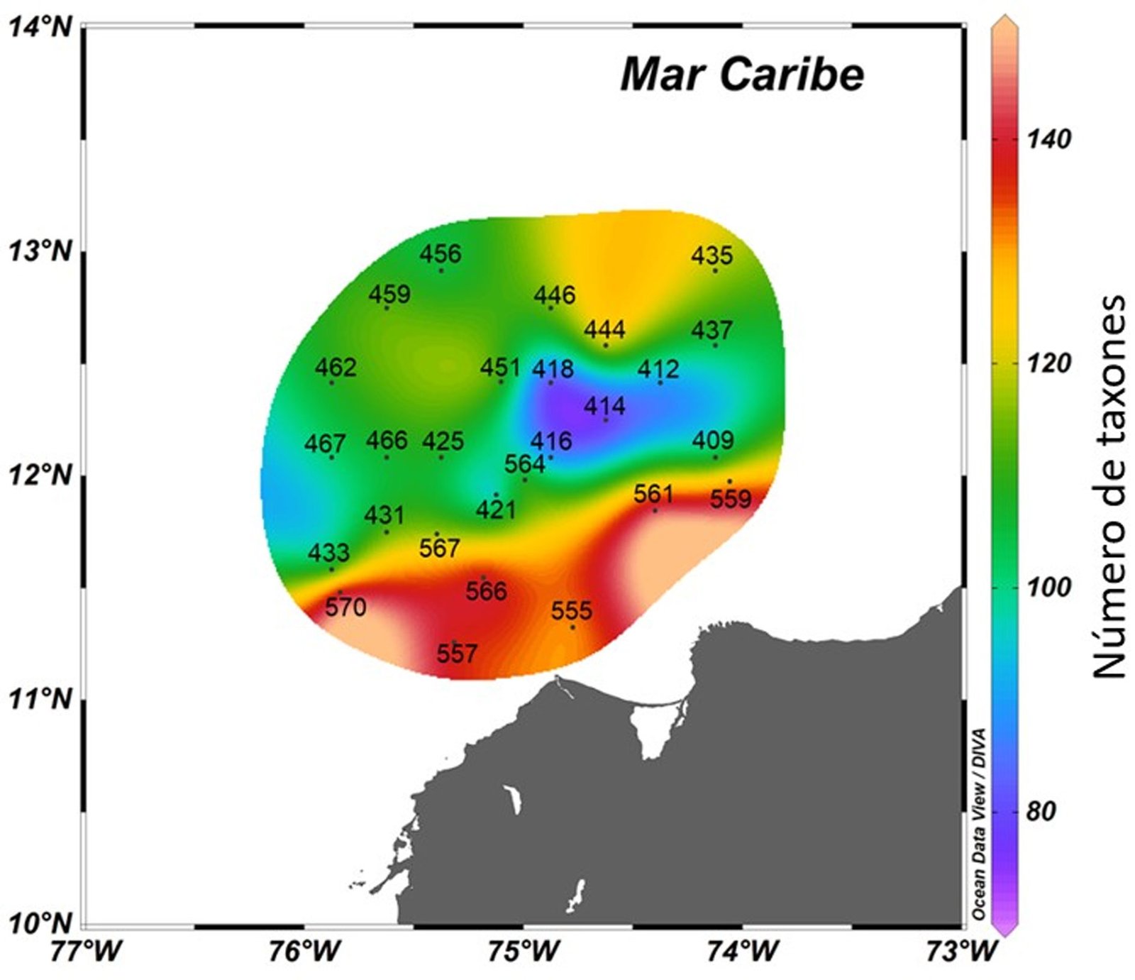
Figura 2.Distribución de la riqueza total del fitoplancton marino en el Caribe central colombiano a partir de las muestras de red y botella.
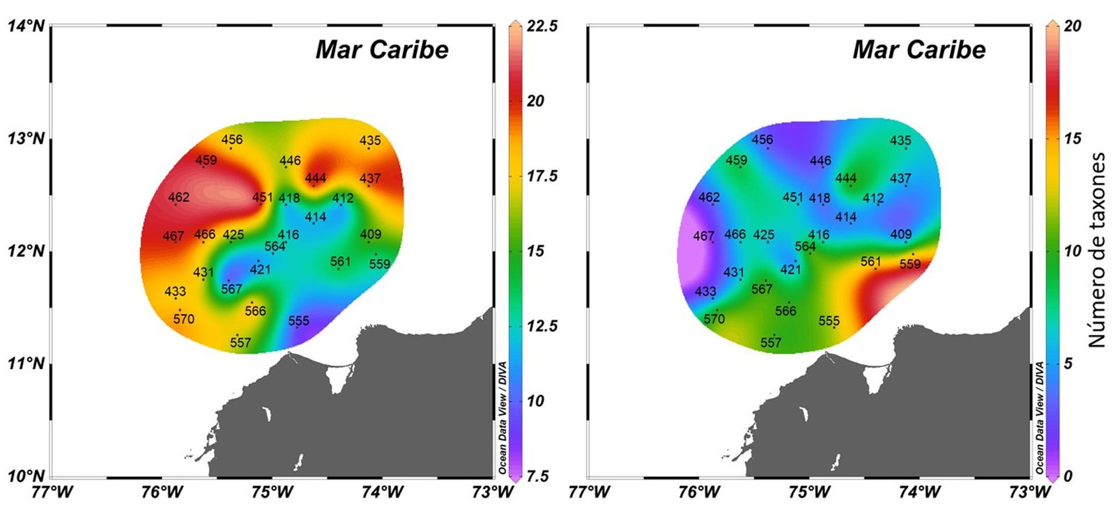
Figura 3.Distribución de la riqueza de especies de los 2 géneros más representativos en el Caribe central colombiano a partir de las muestras de red y botella. A, Dinoflagelados Tripos; B, diatomeas Chaetoceros.
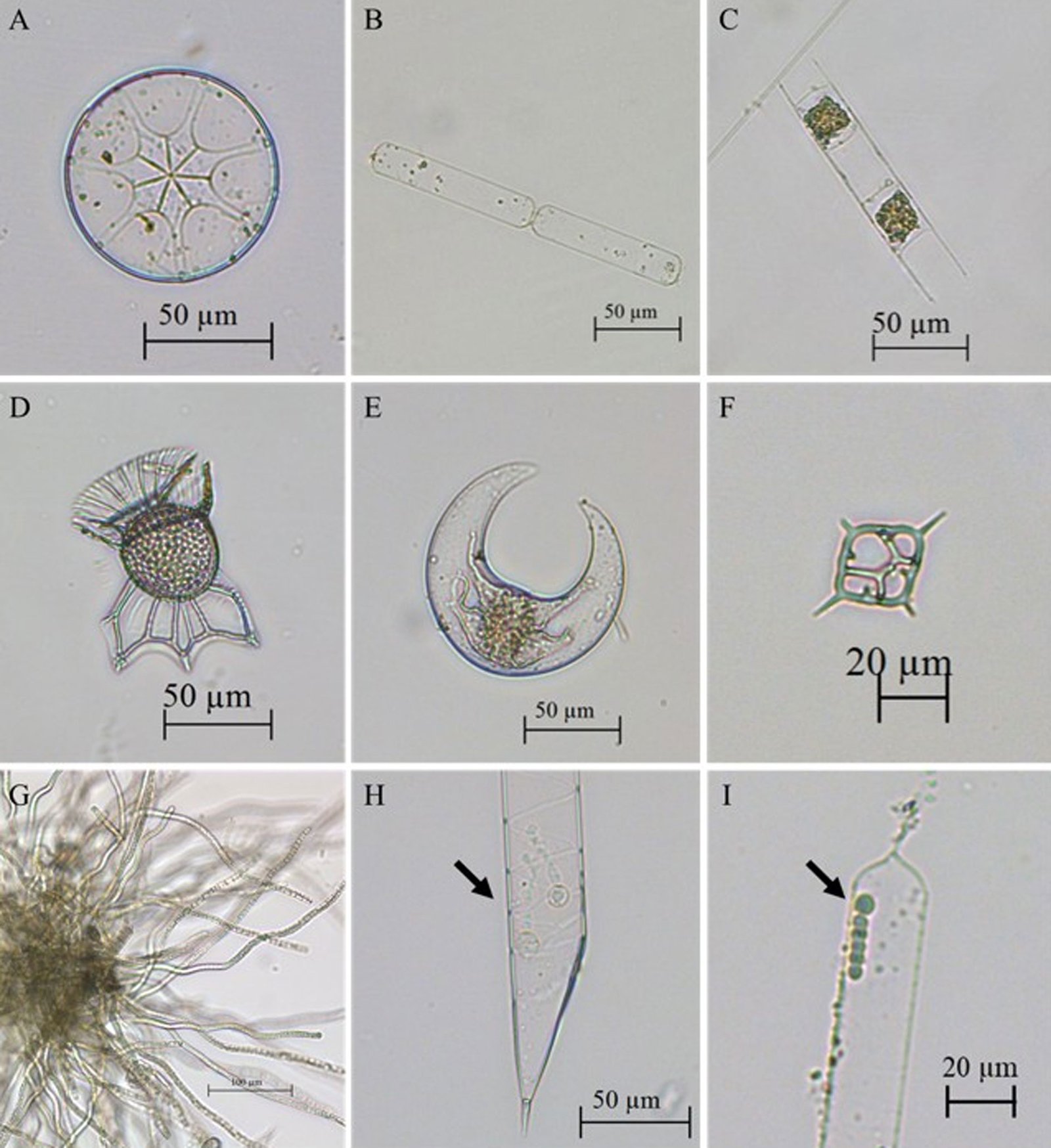
Figura 4. Especies frecuentes registradas en el Caribe central colombiano recolectadas a partir de las muestras de red y botella. A, Asterolampra marylandica (diatomea); B, Cerataulina pelagica (diatomea); C, Hemiaulus hauckii (diatomea); D, Ornithocercus magnificus (dinoflagelado); E, Pyrocystis lunula (dinoflagelado); F, Dictyocha fibula (silicoflagelado); G, Trichodesmium sp. (cianobacteria); H, Richelia intracellularis (cianobacteria) en simbiosis con Rhizosolenia clevei (diatomea);I, Richelia intracellularis (cianobacteria) en simbiosis con Guinardia cylindrus (diatomea).
Por su parte, se registraron 36 taxones raros (registrados en una sola estación) dentro de los que se encuentran los dinoflagelados Amphisolenia bifurcata G. Murray et Whitting, 1899, Brachidinium capitatum F.J.R. Taylor, 1963, Centrodinium maximum Pavillard, 1930, Ceratoperidinium margalefii A.R. Loeblich III, 1980, Citharistes apsteinii F. Schütt, 1895, Corythodinium robustum (Kofoid et J.R. Michener) F. Gómez, 2017, Dinophysis hastata F. Stein, 1883 (fig. 5A), Histioneis biremis F. Stein, 1883, H. crateriformis Stein, 1883, Phalacroma circumcinctum Kofoid et J.R. Michener, 1911, Phalacroma mitra F. Schütt, 1895 (fig. 5B), Prorocentrum rostratum F. Stein, 1883, Pyrocystis lanceolata Schröder, 1900, Tripos arietinus (Cleve) F. Gómez, 2021 (fig. 5C), T. belone (Cleve) F. Gómez, 2021, T. bigelowii (Kofoid) F. Gómez, 2013 (fig. 5D), T. digitatus (F. Schütt) F. Gómez, 2013, T. lanceolatus (Kofoid) F. Gómez, 2013, T. longirostrum (Gourret) Hallegraeff et Huisman, 2020, Kofoidinium sp. Pavillard, 1929, 2 morfoespecies del género Cucumeridinium F. Gómez, P. López-García, H. Takayama et D. Moreira, 2015, y 3 taxones posiblemente del orden Gymnodiniales; también se encontraron las diatomeas Cerataulina bicornis (Ehrenberg) Hasle, 1985, Chaetoceros messanensis Castracane, 1875 (fig. 5E), Trieres chinensis (Greville) Ashworth et E.C. Theriot, 2013 (fig. 5F), Gyrosigma sp. Hassall, 1845, nom. cons.;las cianobacterias Merismopedia elegans A. Braun ex Kützing, 1849, Planktothrix sp. Anagnostidis et Komárek, 1988, Pseudanabaena sp. Lauterborn, 1915, Komvophoron sp. Anagnostidis et Komárek, 1988; las clorofitas Tetradesmus lagerheimii M.J. Wynne et Guiry, 2016,y Pediastrum sp. Meyen, 1829y la carofita Staurastrum sp. Meyen ex Ralfs, 1848.
Con la revisión de los listados de Lozano-Duque et al. (2010b, 2011) y los trabajos publicados posteriormente por Lozano-Duque et al. (2010a), Vidal y Lozano-Duque (2011), Dimar-CIOH (2011), Ayala et al. (2011), Hoyos-Acuña et al. (2019), De la Hoz y Betancur (2019) y Córdoba-Mena et al. (2020) se calcularon en total 328 especies de diatomeas y 185 especies de dinoflagelados; se identificaron en el presente trabajo 74 registros nuevos para el Caribe colombiano que corresponden a 50 especies y 9 géneros de dinoflagelados, 8 especies de diatomeas, 1 especie de cocolitofóridos y 1 phylum, 1 clase, 1 orden , 1 familia, 1 género y 1 especie de bigiros (tabla 3; fig. 6). Se encontró que los géneros con mayor número de nuevos registros para el Caribe colombiano fueron Histioneis Stein, 1883 con 8 especies (fig. 7A-H), Dinophysis Ehrenberg, 1839con 6 especies, Corythodinium Loeblich et A.R. Loeblich, 1966; Oxytoxum Stein, 1883 y Phalacroma F. Stein, 1883con 4 especies cada uno, Pyrocystis Wyville-Thompson, 1876con 3 especies y Tripos (Ehrenberg) F. Gómez, 2013; Torodinium Kofoid et Swezy, 1921; Ornithocercus Stein, 1883; Gonyaulax Diesing, 1866; Citharistes Stein, 1883; Prorocentrum Ehrenberg, 1834; Centrodinium Kofoid, 1907y Amphisolenia Stein, 1883con 2 especies cada uno.
Discusión
La composición específica de las masas de agua reflejó las condiciones del medio, mostrando a las diatomeas y a los dinoflagelados como los grupos representativos, estos últimos los que presentaron mayor riqueza de especies. Estos 2 grupos fitoplanctónicos son dominantes en el mar Caribe y en el Caribe colombiano (Lozano-Duque, Medellín-Mora et al., 2010; Lozano-Duque et al., 2011; Okolodkov, 2003). Las especies de dinoflagelados son consideradas comunes en aguas oceánicas (Okolodkov, 2003), ya que gracias a su fisiología presentan bajos requerimientos de nutrientes y una nutrición variada (autótrofa, heterótrofa y mixotrófica), que les permite adaptarse a aguas oligotróficas (Gamboa-Márquez et al., 1994; Licea et al., 1995), como son las aguas oceánicas del Caribe colombiano (Corredor, 1979); por su riqueza y distribución, reflejan su adaptación a las condiciones del mar abierto (López y Caballero, 1997; Margalef, 1969). Así mismo, diferentes trabajos lo han reportado como el grupo dominante en aguas oceánicas del Caribe colombiano (Ayala-Galván et al., 2018, 2021; Garrido-Linares, Alonso-Carvajal, Rueda et al., 2014; INVEMAR et al., 2017; Lozano-Duque et al., 2010a; Ricaurte-Villota et al., 2018).
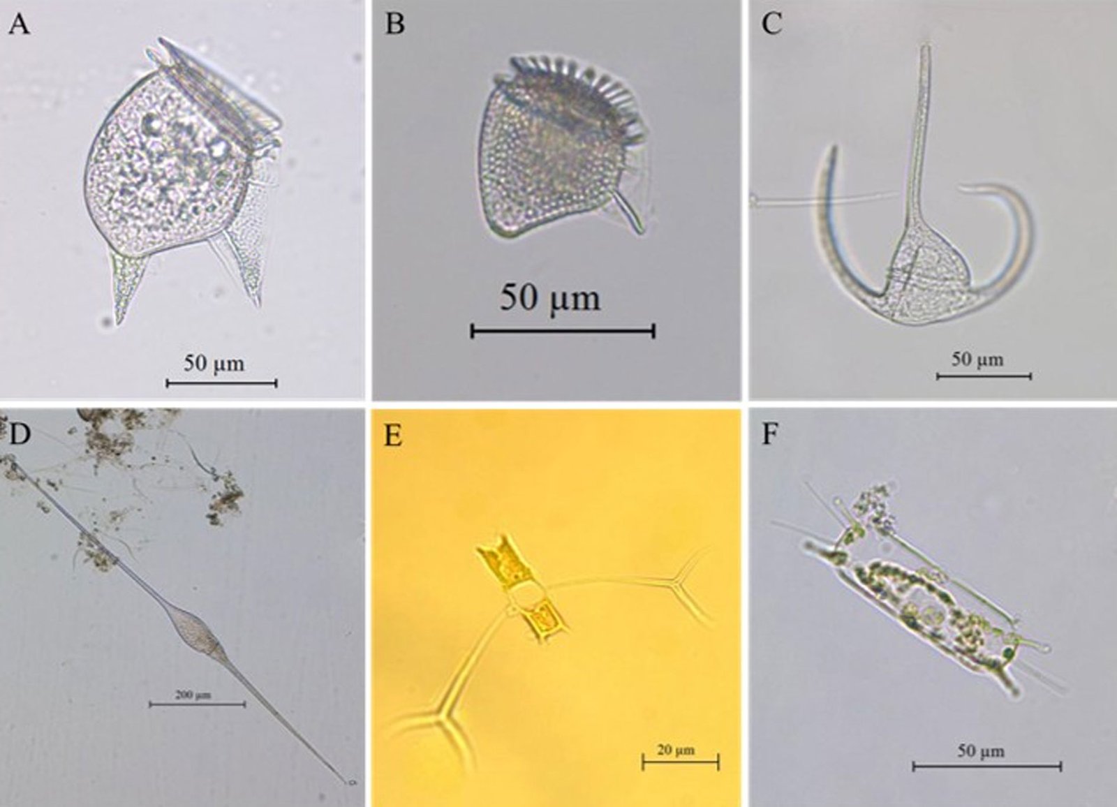
Figura 5.Especies raras registradas en el Caribe central colombiano recolectadas a partir de las muestras de red y botella. A, Dinophysis hastata (dinoflagelado); B, Phalacroma mitra (dinoflagelado); C, Tripos arietinus (dinoflagelado); D, Tripos bigelowii (dinoflagelado); E, Chaetoceros messanensis (diatomea); F, Trieres chinensis (diatomea).
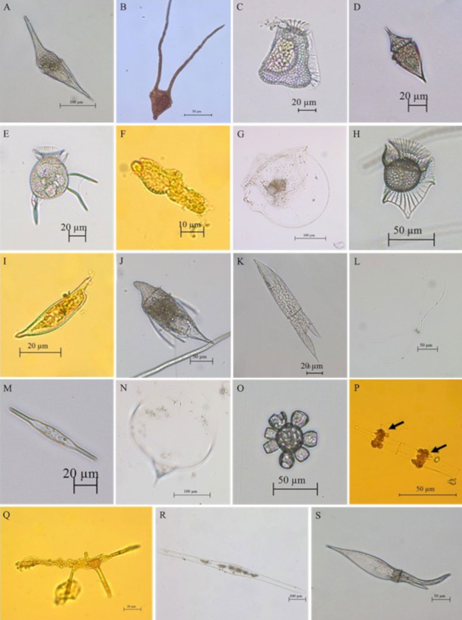
Figura 6. Nuevos registros de especies para el Caribe colombiano recolectados a partir de las muestras de red y botella. A, Centrodinium maximum (dinoflagelado);B, Ceratoperidinium margalefi (dinoflagelado); C, Citharistes apsteinii (dinoflagelado); D, Corythodinium biconicum (dinoflagelado);E, Dinophysis schuettii (dinoflagelado);F, Karenia papilionácea (dinoflagelado);G, Kofoidinium pavillardii (dinoflagelado);H, Ornithocercus carolinae (dinoflagelado);I, Prorocentrum rostratum (dinoflagelado);J, Shuettiella mitra (dinoflagelado);K, Tripos lanceolatus (dinoflagelado);L, Chaetoceros dadayi (diatomea);M, Mastogloia rostrata (diatomea); N, Rhizosolenia debyana (diatomea);O, Scyphosphaera apsteinii (cocolitofórido);P, Solenicola setigera (bigiro);Q, Brachidinium capitatum (dinoflagelado);R, Pyrocystis lanceolata (dinoflagelado);S, Tripos schroeteri (dinoflagelado).
Por su parte, las diatomeas son consideradas más comunes en aguas neríticas (Castillo, 1984; Corchuelo y Moreno, 1983), ya que requieren mayor cantidad de nutrientes y carecen de estructuras especializadas para movilizarse activamente, dependiendo así de los cambios fisicoquímicos diarios de la columna del agua para modificar su posición (Torres y Estrada, 1997). Por ello, han sido reportadas como el grupo dominante en la provincia nerítica de diferentes países (Delgado y Chang, 2010; Loza-Álvarez et al., 2018; Troccoli-Ghinaglia et al., 2004) al igual que en el Caribe colombiano (Franco-Herrera, 2006; Franco-Herrera y Torres-Sierra, 2007; Franco-Herrera et al., 2006; Gavilán et al., 2005; Ramírez-Barón et al., 2010), reflejando su adaptación a condiciones de mayor turbulencia, ya que las favorece a disminuir su sedimentación, y a su vez, se benefician por el aumento en la concentración de nutrientes (Margalef, 1978).
Del grupo de los dinoflagelados, el género Tripos presentó la mayor riqueza, con especies que formaron cadenas de 2 hasta 14 células, como es el caso de algunas especies recolectadas con red como: T. gibberus (Gourret) F. Gómez, 2021 (2 células), T. dens (Ostenfeld et Johannes Schmidt) F. Gómez, 2013 (3 células), T. ranipes (Cleve) F. Gómez, 2013 (4 células) y T. vultur Cleve, 1900(14 células). La formación de cadenas les permite mayor flotabilidad en la zona fótica, generando cadenas más largas en zonas donde la turbulencia es menor (Vargas-Montero et al., 2008). Por lo que estas formaciones están reflejando la estabilidad de la columna de agua, principalmente en el sector externo donde fueron más comunes. La riqueza de Tripos fue mayor hacia aguas más oceánicas, confirmando lo planteado por Lozano-Duque et al. (2010a), quienes teniendo en cuenta estaciones ubicadas a lo largo de un transecto del suroccidente al nororiente a la costa Caribe colombiana, mostró que las aguas oceánicas favorecían la presencia de dinoflagelados, principalmente de este género.
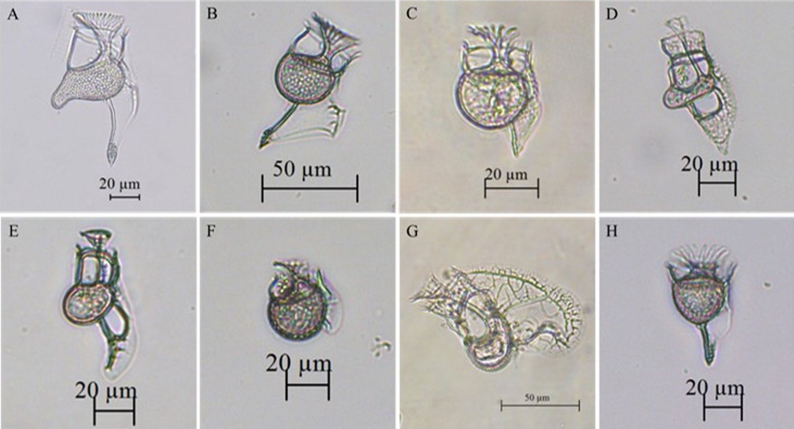
Figura 7. Nuevos registros del género Histioneis para el Caribe colombiano recolectados a partir de las muestras de red y botella. A, Histioneis biremis; B, H. costata; C, H. crateriformis; D, H. depressa; E, H. longicollis; F, H. mediterránea; G, H. milneri; H, H. paraformis.
La presencia de otros géneros de dinoflagelados tecados como Protoperidinium, Ornithocercus, Prorocentrum, Phalacroma, Histioneis y Dinophysis es común en aguas tropicales (Hallegraeff y Jeffrey, 1984; López y Caballero, 1997). Además, indica las estrategias de adaptación que presentan algunos de estos géneros como el tamaño, cuernos y aletas, para asegurar una mayor superficie de absorción, disminuyendo la velocidad de caída y creando dificultad de pastoreo por niveles tróficos superiores (Garay et al., 1988; Hallegraeff y Jeffrey, 1984). Por su parte, aunque el reporte de géneros de dinoflagelados atecados se ve limitado a nivel de caracterización (por su coraza débil) debido a que las técnicas de fijación como formol y lugol dificultan su preservación e identificación (Lalli y Parsons, 1997), se lograron registrar 11 géneros para este grupo. Los géneros de dinoflagelados atecados son conocidos en aguas tropicales, con estudios que se enfocan en análisis moleculares, morfológicos y ecológicos (Escobar-Morales y Hernández-Becerril, 2015; Gómez, 2003, 2005; Gómez y Furuya, 2007; Gómez et al., 2015; Maciel-Baltazar y Hernández-Becerril, 2013), sin embargo, este grupo es mucho menos conocido y estudiado en comparación con los dinoflagelados tecados. Para el Caribe colombiano se encuentran pocos registros resaltando los reportes de los géneros Torodinium Kofoid et Swezy, 1921, Asterodinium Sournia, 1972, Karenia Gert Hansen et Moestrup, 2000, Gyrodinium Kofoid et Swezy, 1921, nom. cons. (Ayala-Galván et al., 2022) y Pronoctiluca Fabre-Domergue, 1889 (Ayala-Galván et al., 2022; Hoyos-Acuña et al., 2019).
Por otra parte, del grupo de las diatomeas, el género Chaetoceros expuso la mayor riqueza;esta diatomea planctónica es un género ampliamente distribuido, es común en ambientes marinos en todo el mundo, ya sea en aguas neríticas u oceánicas, con solo unas pocas especies de ambientes continentales o estuarinos (Sunesen et al., 2008), algunas de sus especies son cosmopolitas (Li et al., 2017) y la mayoría son euritérmicas, eurihalinas y producen hipnosporas (Calderón, 1986), lo que les otorga amplias posibilidades de supervivencia incluso en condiciones adversas (Pitcher, 1990). En este estudio, Chaetoceros disminuyó su riqueza hacia aguas más oceánicas, mostrando que se ven favorecidas con la cercanía hacia aguas neríticas, lo que puede reflejar como esta diatomea se beneficia a mayor turbulencia y concentración de nutrientes (Margalef, 1978), que en este caso estarían dadas en la parte interna del área de estudio, por las descargas continentales del río Magdalena (Restrepo, 2014; Restrepo et al., 2006, 2015).
También se observó la presencia de otros géneros de diatomeas con formas coloniales unidas por prolongacionescomo Skeletonema Greville, 1865, nom. et typ. cons., Pseudo-nitzschia H. Peragallo, 1900, Hemiaulus Heiberg, 1863, nom. cons.y géneros con formas cilíndricas y alargadas como Rhizosolenia; estas formaciones son estrategias que permiten aumentar la relación superficie-volumen mejorando la flotabilidad y favoreciendo la resistencia al hundimiento haciendo que se mantengan en la capa superficial de la columna de agua (Garay et al., 1988).
Con menor riqueza se encontró al grupo de las cianobacterias, con representantes coloniales y filamentosas como: Richelia intracellularis J. Schmidt, 1901, Merismopedia elegans, Oscillatoria limosa C. Agardh ex Gomont, 1892, Planktothrix sp. Anagnostidis et Komárek, 1988, Pseudanabaena sp. Lauterborn, 1915 y Trichodesmium sp.Ehrenberg ex Gomont, 1892, nom. cons.Este grupo es considerado con baja riqueza y frecuencia en aguas marinas en comparación con aguas continentales (Margalef, 1991); sin embargo, estas algas son de gran importancia en ecosistemas oligotróficos (Campos-González, 2007), ya que son capaces de fijar nitrógeno molecular (N2) (Rippka et al., 1979; Stewart, 1980). Las cianobacterias han representado menos de 2% de la composición específica frente al mar Caribe centro de Colombia (Franco-Herrera y Torres-Sierra, 2007), destaca también su baja riqueza en la región insular, pero con altas densidades del género Oscillatoria Vaucher ex Gomont, 1892 (Campos-González, 2007; Garay et al., 1988; INVEMARANH, 2012; Téllez et al., 1988). Este grupo ha mostrado en la provincia nerítica mayor densidad durante la época lluviosa, con representantes estuarinos como Merismopedia Meyen, 1839, Anabaena Bory ex Bornet et Flahault, 1886, nom. cons., Nostoc Vaucher ex Bornet et Flahault, 1886y Oscillatoria Vaucher ex Gomont, 1892(Franco-Herrera et al., 2006).
El género Trichodesmium sp. (fig. 4G) y la especie Richelia intracellularis (fig. 4H, I) presentaron en este estudio una frecuencia de aparición de 78% y 55%, respectivamente,y se consideran relevantes en la composición que presenta el Caribe central colombiano debido a que éstos son los organismos fijadores de N2 (diazótrofos) más importantes de los ambientes pelágicos en los océanos del mundo, pues son responsables de ~ 63% de la fijación de N2 en la zona pelágica (Kulkarni et al., 2010).
Por otra parte, se registraron grupos del fitoplancton marino menos representativos en cuanto a diversidad como los cocolitofóridos (Sournia, 1995; Young et al., 2003), los silicoflagelados (Hernández-Becerril y Bravo-Sierra, 2001; Throndsen, 1997) y grupos más comunes en aguas continentales como las clorofitas (Ehrenberg, 1841), las criptofitas (Cerino y Zingone, 2007) y las carofitas (Brook, 1965). En el área solo se registró a Scyphosphaera apsteinii Lohmann, 1902como representante de los cocolitofóridoscon una frecuencia de aparición de 52% y más común hacia aguas más oceánicas. Los cocolitofóridos pueden encontrarse tanto en aguas neríticas como oceánicas, y la mayoría de sus especies se dan en mares cálidos; mientras que los silicoflagelados, con pocas especies conocidas, generalmente son más abundantes en aguas frías (Lalli y Parsons, 1997). Los cocolitofóridos han mostrado mayor riqueza en aguas oceánicas de otros países como Cuba, donde se encontraron 20 especies (Loza-Álvarez y Lugioyo-Gallardo, 2009) o en el golfo de México con 29 taxones (Gaarder y Hasle, 1971). Para los silicoflagelados solo se registraron 2 representantes, Dictyocha fibula con una frecuencia de aparición de 100% y Octactis octonaria (Ehrenberg) Hovasse, 1946,con 22%, aunque esta última no estuvo presente en el sector externo. Estas especies también han sido registradas para el Pacífico colombiano (Peña y Pinilla, 2002).
Por su parte, las clorofitas y las carofitas son grupos normalmente de aguas continentales o estuarinas que se encontraron en bajas frecuencias y densidades en la provincia oceánica, reflejando la influencia de aguas continentales por corrientes locales principalmente en el sector interno, donde, la especie más común fue la clorofita Pyramimonas longicauda L. Van Meel, 1969. Estos grupos también se han registrado en aguas neríticas y oceánicas del Caribe colombiano con baja representatividad, como se ha demostrado en los estudios de Tigreros (2001) y Franco-Herrera y Torres-Sierra (2007).
En este estudio se encontraron asociaciones simbióticas como la de Solenicola setigera Pavillard, 1916con Dactyliosolen mediterraneus (H. Peragallo) H. Peragallo, 1892, la cualno había sido reportada para el Caribe colombiano. El bigiro S. setigera frecuentemente se encuentra adherido a las valvas de D. mediterraneus, sin embargo, también se puede encontrar formando colonias aisladas (Gómez, 2007; Valencia, 2013), lo que indicaría en ciertos momentos limitaciones de compuestos nitrogenados, especialmente de nitratos (Meave-del Castillo et al., 2012). Otras asociaciones encontradas fueron las de Richelia intracellularis con Guinardia cylindrus (Cleve) Hasle, 1996,o R. intracellularis con Rhizosolenia clevei Ostenfeld, 1902, las cuales ya habían sido reportadas para el Caribe colombiano en el Área de Régimen Común Colombia – Jamaica (INVEMAR-ANH, 2012), Cayo Serranilla (Ricaurte-Villota et al., 2018) y al norte de La Guajira (Ayala-Galván et al., 2018). Se conoce que los hospedadores más comunes de R. intracelularis son diatomeas de los géneros Rhizosolenia, Hemiaulus y Guinardia H. Peragallo, 1892 (Kulkarni et al., 2010). Sin embargo, esta simbiosis es más frecuente con las especies R. clevei y G. cylindrus que se encuentran en aguas tropicales (Hallegraeff y Jeffrey, 1984), así como se pudo observar en este estudio donde fue común encontrar a R. intracellularis con R. clevei. En general, este tipo de asociaciones simbióticas son conocidas y han sido registradas en los mares mundiales (Gárate-Lizárraga y Muñetón-Gómez, 2009; Gómez et al.,2005; Hallegraeff y Jeffrey, 1984; Margalef, 1961; Taylor, 1982; Valencia, 2013). La importancia de éstas en el ambiente marino radica en que pueden beneficiar tanto al huésped como al simbionte mediante el intercambio mutuo de nutrientes orgánicos e inorgánicos (Hallegraeff y Jeffrey, 1984).
La frecuencia de algunas especies encontradas se relaciona con su distribución y amplios rangos de tolerancia, Chaetoceros lorenzianus, C. peruvianus, Cerataulina pelágica, Pseudosolenia calcar-avis, Pyrocystis lunula, Ornithocercus magnificus, Tripos extensus, T. teres, T. trichoceros y Podolampas elegans se consideran cosmopolitas de aguas templadas y cálidas; Hemiaulus hauckii y H. chinensis cosmopolitas de aguas cálidasy Dictyocha fibula cosmopolita euroica(Margalef, 1961). Por su parte, los taxones raros o poco comunes representaron 12.54% de las especies identificadas, 25 de los 36 taxones con un solo registro fueron de dinoflagelados, y mostraron una mayor diversidad en aguas oceánicas, generando un aporte significativo a la estructura fitoplanctónica del Caribe central colombiano.
Al comparar el número de taxones encontrados (176 dinoflagelados y 88 diatomeas) con los registros del Gran Caribe, donde se encuentran alrededor de 1,083 especies de diatomeas (305 diatomeas céntricas y 778 diatomeas pennadas) (Navarro y Hernández-Becerril, 1997) y 404 especies de dinoflagelados (Wood, 1968), el presente trabajo representa, aproximadamente, 17.75% del total de especies conocidas de estos 2 grupos en el Gran Caribe. Al compararlos con los registros del mar Caribe colombiano, donde se han encontrado para aguas oceánicas y costeras un total de 312 especies de diatomeas pertenecientes a 106 géneros y 169 especies de dinoflagelados de 32 géneros (Lozano-Duque et al., 2010b, 2011), el presente trabajo representa aproximadamente 51.46% del total de especies registradas en estudios del mar Caribe colombiano. De lo anterior, si se tiene en cuenta la composición específica, este trabajo generó un aumento para los dinoflagelados de 27.03% (50 especies) y para las diatomeas de 2.44% (8 especies). Cabe anotar que las especies de dinoflagelados Tripos falcatus (Kofoid) F. Gómez, nom. inval. 2013 y Dinophysis capitulata Balech, nom. inválido. 1967, hasta la fecha tampoco se han registrado en el Caribe colombiano, sin embargo, no se incluyeron como nuevos registros debido a que sus estatus taxonómicos están bajo evaluación (Guiry y Guiry, 2025).
Uno de los registros más relevantes fue el de Solenicola setigera, debido a que es un registro nuevo desde la categoría taxonómica de phylum (Bigyra). Este phylum comprende generalmente organismos parásitos o simbiontes. Para aguas oceánicas del Caribe colombiano no se encontraron artículos científicos que confirmen la presencia de éstos. Sin embargo, para Colombia se encontró el registro del phylum asociado con la especie parásita Blastocystis hominis Brumpt 1912 en 2 conjuntos de datos en GBIF (Global Biodiversity Information Facility), publicados por el Instituto Nacional de Salud (Duque et al., 2022, 2023). En cuanto a S. setigera, esun protista marino colonial distintivo y muy extendido (Buck y Bentham, 1998) que no tenía definida su posición filogenética, la cual fue aclarada por Gómez et al. (2011).
Respecto al hallazgo de Scyphosphaera apsteinii, cabe mencionar que esta especie no se encontró registrada en artículos científicos para el Caribe colombiano. Sin embargo, se registra previamente en 2 conjuntos de datos en GBIF que pertenecen a las expediciones de Seaflower del Proyecto Colombia BIO (Ayala-Galván, 2018; Ayala-Galván y Dorado-Roncancio, 2021). Además, el género se encuentra en el listado para aguas oceánicas del Caribe colombiano realizado por Ayala-Galván et al. (2022).
Los resultados obtenidos sugieren que aún queda mucho por explorar respecto a la riqueza de especies en el Caribe colombiano. La información limitada disponible en aguas oceánicas puede estar relacionada con que la mayoría de estudios realizados proviene de cruceros ocasionales. Esta falta de estudios persistentes impide un conocimiento detallado de la composición específica del fitoplancton marino de aguas oceánicas, ya que estas comunidades pueden variar en diferentes escalas temporales (Davidson et al., 2013; Henson et al., 2009; Holligan y Harbour, 1977; Westberry et al., 2016).
El alto número de registros nuevos encontrados podría atribuirse, en parte, a que los resultados de este trabajo respondieron a un análisis a mesoescala, el cual no se había realizado antes para este grupo biológico en un área que representó 7.5% de las aguas oceánicas del Caribe colombiano. Así como a la ubicación del área de estudio, ya que, aunque en su totalidad pertenece a la zona oceánica, abarca estaciones en un gradiente latitudinal que se extiende desde cercanías con la zona nerítica hacia aguas más oceánicas (factor horizontal), con lo que se incrementó la probabilidad de detectar especies raras y menos frecuentes. Además, el esfuerzo de muestreo a 3 profundidades (factor vertical) permitió una mayor captura de organismos, incluyendo aquellos que habitan en diferentes masas de agua como el ASC y el ASS.
En conclusión, estos hallazgos revelan de forma general una alta riqueza fitoplanctónica en aguas oceánicas del Caribe colombiano, la cual fue mayor hacia el sector interno en aguas más cercanas a la costa, probablemente por la influencia del río Magdalena. La riqueza también se vio reflejada en los nuevos registros de dinoflagelados, diatomeas, cocolitofóridos y bigiros, que contribuyeron significativamente al conocimiento de la biodiversidad en el área, especialmente por el primer reporte del phylum Bigyra, así como el alto porcentaje de nuevos registros de dinoflagelados, que confirman su relevancia en aguas costa afuera. Estos resultados destacan la importancia de realizar estudios de composición taxonómica, análisis espaciales a mayor escala (mesoescala > 100 km y macroescala > 1,000 km), que permitan un mayor conocimiento de las comunidades fitoplanctónicas en este complejo ecosistema marino.
Agradecimientos
Se agradece a al Instituto de Investigaciones Marinas y Costeras (INVEMAR) y a la Agencia de Nacional de Hidrocarburos (ANH) de Colombia, por la financiación de los proyectos “Línea base ambiental de los bloques COL 1 y COL 2 en la cuenca sedimentaria del Caribe colombiano fase II temática 1 (convenios 290-2015 y 167 -2016)” y “Estudio técnico ambiental de línea base en el área de evaluación COL 3 sobre la cuenca sedimentaria del Caribe colombiano (convenio 379-2017)”. Esta publicación corresponde a la contribución Núm. 1399 del INVEMAR. Además, damos un sentido agradecimiento al profesor Luis Alfonso Vidal Velásquez (Q. E. P. D.), por su asesoría en la confirmación de las identificaciones. Finalmente, agradecemos a los revisores anónimos por sus valiosos comentarios y sugerencias, los cuales contribuyeron a mejorar este manuscrito.
Referencias
Álvarez-León, R., Aguilera-Quiñones, J., Andrade-Amaya, C. A. y Nowak, P. (1995). Caracterización general de la zona de surgencia en la Guajira colombiana. Revista de la Academia Colombiana de Ciencias Exactas Físicas y Naturales, 19, 679–694.
Andrade, C. A. y Barton, E. D. (2005). The Guajira upwelling system. Continental Shelf Research, 25, 1003–1022. https://doi.org/10.1016/j.csr.2004.12.012
Ávila-Silva, M. Y. (2018). Caracterización del ensamblaje de dinoflagelados en un sector oceánico del Caribe colombiano en la época de lluvias mayor (2015) y seca mayor (2016) (Tesis, Biología). Facultad de Ciencias Básicas, Universidad del Magdalena. Santa Marta, Colombia.
Ayala, C., Martínez, P. A., Méndez, A. y Vidal, L. A. (2011). Primer registro del dinoflagelado Neoceratium digitatum (Schütt) Gómez, Moreira y López-García 2009 (Dinophyceae), en aguas del Caribe colombiano. Biota Colombiana, 12, 145–148.
Ayala-Galván, K. (2018). Composición del fitoplancton en Isla Cayo de Serranilla en la Reserva de Biosfera – Seaflower (Versión 1) [Conjunto de datos]. Instituto de Investigaciones Marinas y Costeras. https://doi.org/10.15472/2bekzn
Ayala-Galván, K. y Dorado-Roncancio, F. (2021). Composición del fitoplancton en la Isla Cayos de Serrana en la Reserva de Biosfera – Seaflower [Conjunto de datos]. Instituto de Investigaciones Marinas y Costeras. https://doi.org/10.15472/hna7kq
Ayala-Galván, K., Dorado, F. y Escarria, E. (2018). Caracterización de comunidades biológicas A. Plancton. En M. Vides y D. Alonso (Eds.), Estudio técnico ambiental de línea base en el área de evaluación COL 10, extremo norte del Caribe colombiano. Informe Técnico Final(pp. 103–173). Agencia Nacional de Hidrocarburos/ Instituto de Investigaciones Marinas y Costeras José Benito Vives de Andréis (Convenio 340-2018).
Ayala-Galván, K., Dorado, F. y Escarria, E. (2021). Plancton. En M. Vides y D. Alonso (Eds.), Estudio técnico ambiental en áreas de interés del Caribe y Pacífico colombiano como apoyo al crecimiento sostenible del sector de hidrocarburos costa afuera – fase 2021. Informe Técnico Final(pp. 121–196). Agencia Nacional de Hidrocarburos/ Instituto de Investigaciones Marinas y Costeras José Benito Vives de Andréis (Convenio 265-2021).
Ayala-Galván, K., Dorado, F., Escarria, E., Gutiérrez, J., Contreras, K., Cárdenas, A. et al. (2017). Caracterización de comunidades biológicas. En M. Vides, M. Santos-Acevedo y D. Alonso (Eds.), Estudio técnico ambiental de línea base en el área de evaluación COL 3 sobre la cuenca sedimentaria del Caribe colombiano. Informe Técnico Final (pp. 98–260). Agencia Nacional de Hidrocarburos/ Instituto de Investigaciones Marinas y Costeras José Benito Vives de Andréis (Convenio 379-2017).
Ayala-Galván, K. y Gutiérrez-Salcedo, J. M. (2019). Comunidades biológicas: plancton. En M. Vides y D. Alonso (Eds.), Integración, análisis y diagnóstico de información de línea base ambiental de la cuenca Caribe como apoyo a nuevas a fronteras del desarrollo del sector de hidrocarburos costa afuera. Informe Técnico Final (pp. 209–256). Agencia Nacional de Hidrocarburos/ Instituto de Investigaciones Marinas y Costeras José Benito Vives de Andréis (Convenio 399-2019).
Ayala-Galván, K., Gutiérrez-Salcedo, J. M. y Montoya-Cadavid, E. (2022). Fitoplancton de la provincia oceánica del mar Caribe colombiano. Diez años de historia. Biota Colombiana, 23, e903. https://doi.org/10.21068/2539200X.903
Balech, E. (1988). Los dinoflagelados del Atlántico sudoccidental. Publicación especial del Instituto Español de Oceanografía. Consejo Regional de Asturias.
Bernal, G., Poveda, G., Roldan, P. y Andrade, C. (2006). Patrones de variabilidad de las temperaturas superficiales del mar en la Costa Caribe colombiana. Revista de la Academia Colombiana de Ciencias Exactas, Físicas y Naturales, 30, 195–208. https://doi.org/10.18257/raccefyn.30(115).2006.2240
Boltovskoy, D. (1981). Atlas del zooplancton del Atlántico sudoccidental y métodos de trabajo con el zooplancton marino. Mar del Plata, Argentina: INIDEP (Instituto Nacional de Investigación y Desarrollo Pesquero).
Brook, A. J. (1965). Planctonic algae as indicators of lakes types with special reference to the Desmidiaceae. Limnology and Oceanography, 10, 403–411. https://doi.org/10.4319/lo.1965.10.3.0403
Buck, K. R. y Bentham, W. N. (1998). A novel symbiosis between a cyanobacterium, Synechococcus sp., an aplastidic protist, Solenicola setigera, and a diatom, Leptocylindrus mediterraneus, in the open ocean. Marine Biology, 132, 349–355. https://doi.org/10.1007/s002270050401
Calderón, E. (1986). Las diatomeas en el plancton de los esteros de la rada de Tumaco (Pacífico colombiano), con observaciones ecológicas y biogeográficas (Tesis, Biología Marina). Facultad de Ciencias Naturales e Ingeniería, Universidad de Bogotá Jorge Tadeo Lozano.
Campos-González, E. (2007). Fitoplancton de las islas de Providencia y Santa Catalina, Caribe colombiano (Tesis, Biología Marina) Facultad de Ciencias Naturales Ingeniería, Universidad de Bogotá Jorge Tadeo Lozano.
Castillo, F. (1984). Fitoplancton del Pacífico colombiano como indicador de masas de agua (ERFEN IV). Biología Pesquera, 13, 67–70.
Cerino, F. y Zingone, A. (2007). Decrypting cryptomonads: a challenge for molecular taxonomy. En J. Brodie y J. Lewis (Eds.), Unravelling the algae: the past, present, and future of algal systematics (pp. 197–214). Systematics Association Special Volume Series, 75. Boca Raton: CRC Press.
Clarke, K. y Gorley, R. N. (2015). PRIMER (Plymouth routines in multivariate ecological research) v7. User manual/tutorial. PRIMER-E, Plymouth Marine Laboratory.
Corchuelo, M. y Moreno, G. (1983). Contribución al conocimiento del fitoplancton y algunos tintínidos del Pacífico colombiano (Tesis, Biología Marina). Facultad de Ciencias Naturales e Ingeniería, Universidad de Bogotá Jorge Tadeo Lozano.
Córdoba-Mena, N., Florez-Leiva, L., Atehortúa, L. y Obando, E. (2020). Changes in phytoplankton communities in a tropical estuary in the Colombian Caribbean Sea. Estuaries and Coasts, 43, 2106–2127. https://doi.org/10.1007/s12237-020-00750-z
Corredor, J. E. (1979). Phytoplankton response to low level nutrient enrichment through upwelling in the Columbian Caribbean Basin. Deep Sea Research Part A: Oceanographic Research Papers, 26, 731–741. https://doi.org/10.1016/0198-0149(79)90010-4
Cupp, E., (1943). Marine plankton diatoms of the west coast of North America. Bulletin of the Scripps Institution of Oceanography of the University of California, 5, 1–238.
Davidson, K., Gilpin, L. C., Pete, R., Brennan, D., McNeill, S., Moschonas, G. et al. (2013). Phytoplankton and bacterial distribution and productivity on and around Jones Bank in the Celtic Sea. Progress in Oceanography, 117, 48–63. https://doi.org/10.1016/j.pocean.2013.04.001
De la Hoz, L. A. y Betancur, S. P. (2019). Nuevo registro de la especie Cladopyxis hemibrachiata del grupo dinoflagelado para la reserva de la biosfera de Seaflower, Caribe colombiano. Boletín Científico CIOH, 38, 41–43. https://doi.org/10.26640/22159045.2019.466
Delgado, L. E. y Chang, F. (2010). La comunidad microalgal durante el verano 2006. Instituto del Mar Perú, 36, 3–4.
Dimar-CIOH. (2011). Catálogo de fitoplancton de la Bahía de Cartagena, Bahía Portete y Agua de Lastre. Dirección General Marítima Centro de Investigaciones Oceanográficas e Hidrográficas del Caribe. Serie de Publicaciones Especiales CIOH, 5. https://doi.org/10.26640/52.2011
Dorado-Roncancio, E. F., Medellín-Mora, J., Mancera-Pineda, J. E. y Pizarro-Koch, M. (2022). Copepods of the off-shore waters of Caribbean Colombian Sea and their response to oceanographic regulators. Journal of the Marine Biological Association of the United Kingdom, 101, 1129–1143. https://doi.org/10.1017/S0025315422000133
Duque, S., Arévalo-Jamaica, A., Gunturiz-Albarracín, M. L., Figueroa-Velandia, S. y López-Hernández, R. G. (2022). Colección de giardiasis del Instituto Nacional de Salud (Versión 1.1) [Conjunto de datos]. Instituto Nacional de Salud. Dataset/ Occurrence. https://doi.org/10.15472/68g8jh
Duque, S., Arévalo-Jamaica, A., Gunturiz-Albarracín, M. L., Figueroa-Velandia, S. y López-Hernández, R. G. (2023). Biobanco de parásitos intestinales del Instituto Nacional de Salud (Versión 1.2) [Conjunto de datos]. Instituto Nacional de Salud. Dataset/Occurrence. https://doi.org/10.15472/zoth79
Edler, L. y Elbrächter, M. (2010). The Utermöhl method for quantitative phytoplankton analysis. Microscopic and Molecular Methods for Quantitative Phytoplankton Analysis, 110, 13–20.
Ehrenberg, C. G. (1841). Verbreitung und Einflus des mikroskopischen Lebens in Sud-und Nord-Amerika. Abhandlungen der Königlichen Akademie der Wissenschaften zu Berlin, Physik. Kl., 1841, 291–445.
Escobar-Morales, S. y Hernández-Becerril, D. U. (2015). Free-living marine planktonic unarmoured dinoflagellates
from the Mexican tropical Pacific. Acta Botanica Mexicana, 110, 93–123. https://doi.org/10.1515/bot-2014-0049
Franco-Herrera, A. (2006). Variación estacional del fitoplancton y mesozooplancton e impacto de herbivoría de Eucalanus subtenuis, Giesbrecht, 1888 (Copepoda: Eucalanidae) en el Caribe colombiano (Tesis doctoral, en Oceanografía). Facultad de Ciencias Naturales y Oceanográficas, Universidad de Concepción. Chile.
Franco-Herrera, A., Castro, L. y Tigreros, P. (2006). Plankton dynamics in the south-central Caribbean Sea: strong seasonal changes in the Coastal Tropics Sytems. Caribbean Journal of Science, 42, 24–28.
Franco-Herrera, A. y Torres-Sierra, E. A. (2007). La comunidad fitoplanctónica en el evento de surgencia frente al mar Caribe centro de Colombia. Actualidades y Divulgación Científica, 10, 159–172. https://doi.org/10.31910/rudca.v10.n1.2007.578
Gaarder, K. R. y Hasle, G. R. (1971). Coccolithophorids of the Gulf of Mexico. Bulletin of Marine Science, 21, 519–544.
Gamboa-Márquez, J. F., Sánchez-Suárez, I. G. y La Barbera-Sánchez, A. (1994). Dinoflagelados (Pyrrophyta) del Archi-
piélago Los Roques (Venezuela): familias Prorocentraceae y Ostreopsidaceae. Acta Científica Venezolana, 45, 140–152.
Gárate-Lizárraga I. y Muñetón-Gómez M. (2009). Primer registro de la diatomea epibionte Pseudohimantidium pacificum y de otras asociaciones simbióticas en el golfo de California. Acta Botanica Mexicana, 88, 31–45. https://doi.org/10.21829/abm88.2009.311
Garay, J., Castillo, F., Andrade, C., Aguilera, J., Niño, L., De La Pava, M. et al. (1988). Estudio oceanográfico del área insular y oceánica del Caribe colombiano – archipiélago de San Andrés y Providencia y cayos vecinos. Boletín Científico CIOH, 9, 3–73. https://doi.org/10.26640/01200542.8.3_73
Garrido-Linares, M., Alonso-Carvajal, D., Gutiérrez-Salcedo, J. M., Montoya-Cadavid, E., Rodríguez, A., Bastidas, M. et al. (2014). Línea base ambiental preliminar del bloque de exploración de hidrocarburos Guajira Offshore 3 en el Caribe colombiano. Informe técnico Final. Agencia Nacional de Hidrocarburos/ Instituto de Investigaciones Marinas y Costeras José Benito Vives de Andréis (Convenio 171–2013).
Garrido-Linares, M., Alonso-Carvajal, D., Rueda, M., Ricaurte, C., Polanco, A., Cárdenas, A. et al. (2014). Línea base ambiental preliminar de los bloques de exploración de hidrocarburos Caribe colombiano: fase COL 4 y COL 5. Informe técnico Final Agencia Nacional de Hidrocarburos/ Instituto de Investigaciones Marinas y Costeras José Benito Vives de Andréis (Convenio 188–2014).
Gavilán, M., Cañón, M. y Tous, G. (2005). Comunidad fitoplanctónica de la Bahía de Cartagena y en las aguas de lastre de buques de tráfico internacional. Boletín Científico CIOH, 23, 60–75. https://doi.org/10.26640/01200542.23.60_75
Gómez, F. (2003). New records of Asterodinium Sournia (Brachidiniales, Dinophyceae). Acta Botanica Croatica, 62, 85–92. https://doi.org/10.1127/0029-5035/2003/0077-0331
Gómez, F. (2005). Is Karenia a synonym of Asterodinium-Brachidinium (Gymnodiniales, Dinophyceae)? Vie et Milieu, 55, 237–242.
Gómez, F. (2007). The consortium of the protozoan Solenicola setigera and the diatom Leptocylindrus mediterraneus in the Pacific Ocean. Acta Protozoologica, 46, 15–24.
Gómez, F. y Furuya, K. (2007). Kofoidinium, Spatulodinium and other kofoidiniaceans (Noctilucales, Dinophyceae) in the Pacific Ocean. European Journal of Protistology, 43, 115–124. https://doi.org/10.1016/j.ejop.2006.12.002
Gómez, F., Furuya, Y. y Takeda, S. (2005). Distribution of the Cyanobacterium Richelia intracellularis as an epiphyte of the diatom Chaetoceros compresssus in the Western Pacific Ocean. Journal of Plankton Research, 27, 323–330. https://doi.org/10.1093/plankt/fbi007
Gómez, F., López-García, P., Takayama, H. y Moreira, D. (2015). Balechina and the new genus Cucumeridinium gen. nov. (Dinophyceae), unarmored dinoflagellates with thick cell coverings. Journal of Phycology, 51, 1088–1105. https://doi.org/10.1111/jpy.12346
Gómez, F., Moreira, D., Benzerara, K. y López-García, P. (2011). Solenicola setigera is the first characterized member of the abundant and cosmopolitan uncultured marine stramenopile group MAST-3. Environmental Microbiology, 13, 193–202. https://doi.org/10.1111/j.1462-2920.2010.02320.x
Guiry, M. D. y Guiry, G. M. (2025). AlgaeBase. Publicación electrónica mundial, Universidad Nacional de Irlanda, Galway. Consultado el 24 de febrero de 2025 en https://www.algaebase.org
Hallegraeff, G. M. y Jeffrey, S. W. (1984). Tropical phytoplankton species and pigments of continental shelf waters of north and north-west Australia. Marine Ecology Progress Series, 20, 59–74.
Henson, S. A., Dunne, J. P. y Sarmiento, J. L. (2009). Decadal variability in North Atlantic phytoplankton blooms. Journal of Geophysical Research: Oceans, 114, C04013. https://doi.org/10.1029/2008JC005139
Hernández-Becerril, D. U. y Bravo-Sierra, E. (2001). Planktonic silicoflagellates (Dictyochophyceae) from the Mexican Pacific. Botanica Marina, 44, 417–423. https://doi.org/10.1515/BOT.2001.050
Holligan, P. M. y Harbour, D. S. (1977). The vertical distribution and succession of phytoplankton in the western English Channel in 1975 and 1976. Journal of the Marine Biological Association of the United Kingdom, 57, 1075–1093. https://doi.org/10.1017/S002531540002614X
Hoppenrath, M., Elbrächter, M. y Drebes, G. (2009). Marine phytoplankton. Stuttgart:Kleine SenckenbergReihe.
Hoyos-Acuña, J. J., Salón-Barros, J. C. y Mancera-Pineda, J. E. (2019). Aspectos morfológicos y primer registro del dinoflagelado Pronoctiluca spinifera en el Caribe colombiano. Acta Biológica Colombiana, 24, 264–274. https://doi.org/10.15446/abc.v24n2.70179
INVEMAR (Instituto de Investigaciones Marinas y Costeras José Benito Vives de Andréis). (2015). Informe del estado de los ambientes y recursos marinos y costeros en Colombia: Año 2014. Serie de Publicaciones Periódicas Núm. 3. Santa Marta, Colombia: INVEMAR.
INVEMAR (Instituto de Investigaciones Marinas y Costeras José Benito Vives de Andréis)-ANH (Agencia Nacional de Hidrocarburos). (2008). Especies, ensamblajes y paisajes de los bloques marinos sujetos a exploración de hidrocarburos. Informe técnico final. Santa Marta, Colombia: Agencia Nacional de Hidrocarburos/ Instituto de Investigaciones Marinas y Costeras José Benito Vives de Andréis.
INVEMAR (Instituto de Investigaciones Marinas y Costeras José Benito Vives de Andréis)-ANH (Agencia Nacional de Hidrocarburos). (2010). Especies, ensamblajes y paisajes de los bloques marinos sujetos a exploración de hidrocarburos – Fase II – Caracterización de la megafauna y el plancton del Caribe colombiano. Informe Técnico Final. Santa Marta, Colombia: Agencia Nacional de Hidrocarburos/ Instituto de Investigaciones Marinas y Costeras José Benito Vives de Andréis.
INVEMAR (Instituto de Investigaciones Marinas y Costeras José Benito Vives de Andréis)-ANH (Agencia Nacional de Hidrocarburos). (2012). Línea base ambiental en el Área de Régimen Común Jamaica – Colombia como aporte al aprovechamiento sostenible de los recursos marinos compartidos. Informe técnico final. Santa Marta, Colombia: Agencia Nacional de Hidrocarburos/ Instituto de Investigaciones Marinas y Costeras José Benito Vives de Andréis.
INVEMAR (Instituto de Investigaciones Marinas y Costeras José Benito Vives de Andréis), CORALINA (Corporación para el Desarrollo Sostenible del Archipiélago de San Andrés, Providencia y Santa Catalina), UNIANDES (Universidad De Los Andes) y UPB (Universidad Pontificia Bolivariana). (2017). Evaluación física y biológica de los ambientes profundos de la isla Cayos de Serrana en la Reserva de Biósfera – Seaflower. Informe Técnico Final. Expedición Científica Seaflower en Isla Cayo Serrana. Santa Marta, Colombia: Instituto de Investigaciones Marinas y Costeras José Benito Vives de Andréis.
Kulkarni, V. V., Chitari, R. R., Narale, D. D., Patil, J. S. y Anil, A. C. (2010). Occurrence of cyanobacteria-diatom symbiosis in the Bay of Bengal: implications in biogeochemistry. Current Science, 99, 6–25.
Lalli, C. y Parsons, T. R. (1997). Biological oceanography: an introduction (2nd Ed.). Elsevier Butterworth-Heinemann.
Li, Y., Boonprakob, A., Gaonkar, C. C., Kooistra, W. H., Lange, C. B., Hernández-Becerril, D. et al. (2017). Diversity in the globally distributed diatom genus Chaetoceros (Bacillariophyceae): three new species from warm-temperate waters. Plos One, 12, e0168887. https://doi.org/10.1371/journal.pone.0168887
Licea, S., Moreno, J. L., Santoyo, H. y Figueroa, G. (1995). Dinoflagelados del golfo de California. La Paz, México:Universidad Autónoma de Baja California Sur.
López, N. O. y Caballero, O. G. (1997). Dinoflagelados del mar peruano como indicadores de masas de agua durante los años 1982 a 1985. Boletín Instituto del Mar del Perú, 16, 1–60.
Loza-Álvarez, S., Benavides-Morera, R., Brenes-Rodríguez, C. L. y Saxon, D. B. (2018). Phytoplankton structure in dry and rainy seasons in the gulf of Papagayo, Costa Rica. Journal of Marine and Coastal Sciences, 10, 9–30. https://doi.org/10.15359/revmar.10-2.1
Loza-Álvarez, S. y Lugioyo-Gallardo, G. M. (2009). Diversidad del microfitoplancton en las aguas oceánicas alrededor de Cuba. Revista Ciencias Marinas y Costeras, 1, 29–47. https://doi.org/10.15359/revmar.1.2
Lozano-Duque, Y., Medellín-Mora, J. y Navas, G. R. (2010). Contexto climatológico y oceanográfico del mar Caribe colombiano. Biodiversidad del margen continental del Caribe colombiano. Santa Marta, Colombia:Serie de publicaciones especiales INVEMAR.
Lozano-Duque, Y., Vidal, L. A. y Navas, G. R. (2011). Lista de especies de dinoflagelados (Dinophyta) registrados en el mar Caribe colombiano. Boletín de Investigaciones Marinas y Costeras-INVEMAR, 40, 361–380.
Lozano-Duque, Y., Vidal, L. A. y Navas, G. R. (2010a). La comunidad fitoplanctónica en el mar Caribe colombiano. Biodiversidad del margen continental del Caribe colombiano. Serie de publicaciones especiales INVEMAR Núm. 20.
Lozano-Duque, Y., Vidal, L. A. y Navas, G. R. (2010b). Listado de diatomeas (Bacillariophyta) registradas para el Mar Caribe colombiano. Boletín de Investigaciones Marinas y Costeras-INVEMAR, 39, 83–116.
Maciel-Baltazar, E. y Hernández-Becerril, D. U. (2013). Especies de dinoflagelados atecados (Dinophyta) de la costa de Chiapas, sur del Pacífico mexicano. Revista de Biología Marina y Oceanografía, 48, 245–259. https://doi.org/10.4067/S0718-19572013000200005
Margalef, R. (1961). Distribución ecológica y geográfica de las especies del fitoplancton marino. Investigación Pesquera, 19, 81–101.
Margalef, R. (1969). Estudios sobre la distribución a pequeña escala del fitoplancton marino. Memorias de la Real Academia de Ciencias y Artes de Barcelona, 40,3–22.
Margalef, R. (1978). Life-forms of phytoplankton as survival alternatives in an unstable environment. Oceanologica Acta, 1, 493–509.
Margalef, R. (1991). Ecología. Barcelona, España: Omega.
Meave-del Castillo, M. E., Zamudio-Reséndiz, M. E. y Castillo-Rivera, M. (2012). Riqueza fitoplanctónica de la bahía de Acapulco y zona costera aledaña, Guerrero, México. Acta Botanica Mexicana, 100, 405–487. https://doi.org/10.21829/abm100.2012.41
Molina, A., Molina, C., Giraldo, L., Parra, C. y Chevillot, P. (1994). Dinámica marina y sus efectos sobre la geomorfología del golfo de Morrosquillo. Boletín Científico CIOH, 15, 93–113. https://doi.org/10.26640/22159045.74
Navarro, J. N. y Hernández-Becerril, D. U. (1997). Check-list of marine diatoms from the Caribbean Sea. Listados Florísticos de México, 15, 1–48.
Okolodkov, Y. B. (2003). A review of Russian plankton research in the Gulf of Mexico and the Caribbean Sea in the 1960-1980s. Hidrobiológica, 13, 207–221.
Peña, V. y Pinilla, G. A. (2002). Composición, distribución y abundancia de la comunidad fitoplanctónica de la ensenada de Utría, Pacífico colombiano. Revista de Biología Marina y Oceanografía, 37, 67–81. http://dx.doi.org/10.4067/S0718-
19572002000100008
Pitcher, G. (1990). Phytoplankton see populations of the Cape Peninsula upwelling plume, with particular reference to resting spores of Chaetoceros (Bacillariophyceae) and their role in seeding upwelling waters. Estuarine, Coastal and Shelf Science, 31, 283–301. https://doi.org/10.1016/0272-7714(90)90105-Z
Ramírez, A. (1999). Ecología aplicada: diseño y análisis estadístico. Bogotá: Fundación Universidad de Bogotá Jorge Tadeo Lozano.
Ramírez-Barón, J. S., Franco-Herrera, A., García-Hoyos, L. M. y López, D. A. (2010). La comunidad fitoplanctónica durante eventos de surgencia y no surgencia, en la zona costera del departamento del Magdalena, Caribe colombiano. Boletín de Investigaciones Marinas y Costeras-INVEMAR, 39, 233–263.
Restrepo, J. C. (2014). Dinámica sedimentaria en deltas micromareales-estratificados de alta descarga: delta del río Magdalena (Colombia-Mar Caribe) (Tesis doctoral, en Ciencias del Mar). Facultad de Ciencias Básicas, Universidad del Norte. Colombia.
Restrepo, J. C., Ortiz, J. C., Otero, L. y Ospino, S. R. (2015). Transporte de sedimentos en suspensión en los principales ríos del Caribe colombiano: magnitud, tendencias y variabilidad. Revista de la Academia Colombiana de Ciencias Exactas, Físicas y Naturales, 39, 527–546. https://doi.org/10.18257/raccefyn.209
Restrepo, J. D., Kjerfve, B., Hermelín, M. y Restrepo, J. C. (2006). Factors controlling sediment yield in a major South American drainage basin: the Magdalena River, Colombia. Journal of Hydrology, 316, 213–232. https://doi.org/10.1016/j.jhydrol.2005.05.002
Ricaurte-Villota, C. y Bastidas-Salamanca, M. L. (Eds.). (2017). Regionalización oceanográfica: una visión dinámica del Caribe. Serie de Publicaciones Especiales Núm.14. Santa Marta, Colombia: Instituto de Investigaciones Marinas y Costeras José Benito Vives De Andréis.
Ricaurte-Villota, C., Murcia-Riaño, M., Ayala-Galván., K., Dorado, E. F., Escarria, E. y Alonso, D. A. (2018). Evaluación física y biológica de los ambientes profundos de la isla cayo de Serranilla en la Reserva de la Biosfera – Seaflower. Expedición Científica Seaflower 2017 Isla Cayo Serranilla. Santa Marta, Colombia: Informe Técnico Final del Instituto de Investigaciones Marinas y Costeras José Benito Vives De Andréis para la Comisión Colombiana del Océano.
Rippka, R. Deruelles, J., Waterbury, J. B., Herdman, M. y Stanier, R. Y. (1979). Generic assignments, strain histories and properties of pure cultures of cyanobacteria. Microbiology, 111, 1–61. https://doi.org/10.1099/00221287-111-1-1
Round, F. (1990). Diatoms: the biology and morphology of the genera. Cambridge: Cambridge University Press. https://doi.org/10.1017/S0025315400059245
Salón, J. C. (2013). Caracterización de la comunidad fitoplanctónica en áreas oceánicas del Caribe colombiano durante la época seca del año 2011 (febrero y marzo) (Tesis, Biología). Facultad de Ciencias Básicas, Universidad del Magdalena. Santa Marta, Colombia.
Schlitzer, R. (2022). Ocean data view. https://odv.awi.de
Sournia, A. (1995). Red tide and toxic marine phytoplankton of the world ocean: and inquiry into biodiversity. En P. Lassus et al. (Eds.), Harmful marine algal blooms (pp. 103–112). París, Francia: Lavoisier.
Stewart, W. D. P. (1980). Some aspects of structure and function in N2-fixing cyanobacteria. Annual Review of Microbiology, 34, 497–536. https://doi.org/10.1146/annurev.mi.34.100180.002433
Sunesen, I., Hernández-Becerril, D. U. y Sar, E. A. (2008). Marine diatoms from Buenos Aires coastal waters (Argentina). V. Species of the genus Chaetoceros. Revista de Biología Marina y Oceanografía, 43, 303–326. https://doi.org/10.4067/S0718-19572008000200009
Taylor, F. J. R. (1976). Dinoflagellates from the International Indian Ocean Expedition. A material collected by the R.V.” Anton Bruun” 1963-1964. Stuttgart, Alemania: Biblioteca Botánica.
Taylor, F. J. R. (1982). Symbioses in marine microplankton. Annales de l’Institut Océanographique, 58, 61–90.
Téllez, C., Márquez, G. y Castillo, F. (1988). Fitoplancton y ecología pelágica en el archipiélago de San Andrés y Providencia: Crucero Océano VI en el Caribe colombiano. Boletín Científico CIOH, 8, 3–26. https://doi.org/10.26640/22159045.26
Throndsen, J. (1997). The planktonic marine flagellates. En C. R. Tomas (Ed.), Identifying marine phytoplankton (pp. 591–729). San Diego, EUA: Academic Press.
Tigreros, P. (2001). Biodiversidad y valoración bioquímica del fitoplancton marino en ambientes costeros mesotróficos y oligotróficos tropicales, Caribe colombiano (Tesis, Biología Marina), Facultad de Ciencias Naturales e Ingeniería, Universidad de Bogotá Jorge Tadeo Lozano.
Tomas, C. (1997). Identifying marine phytoplankton. San Diego, EUA: Academic Press. https://doi.org/10.1017/S0025315400038959
Torres, R. y Estrada, M. (1997). Patrones de migración vertical en el plancton de un lago tropical. Hidrobiológica, 7, 33–40.
Troccoli-Ghinaglia, L., Herrera-Silveira, J. A. y Comín, F. A. (2004). Structural variations of phytoplankton in the coastal seas of Yucatan, Mexico. Hydrobiologia, 519, 85–102. https://doi.org/10.1023/B:HYDR.0000026487.78497.b6
Valencia, V. J. (2013). Variación estacional del fitoplancton en una estación nerítica del Canal de Mallorca (Mediterráneo occidental): 2000-2001 (Tesis doctoral). Departamento de Bioloxía Celular e Molecular de la Facultade de Ciencias, Universidad da Coruña. España.
Vargas-Montero, M., Bustamante, E. F., Guzmán, J. C. y Vargas, J. C. (2008). Florecimientos de dinoflagelados nocivos en la costa Pacífica de Costa Rica. Hidrobiológica, 18, 15–23.
Vidal, L. A. (2010). Manual del fitoplancton hallado en la ciénaga Grande de Santa Marta y cuerpos de agua aledaños. Fundación Universidad de Bogotá Jorge Tadeo Lozano. Bogotá, Colombia.
Vidal, L. A. y Lozano-Duque, Y. (2011). Revisión de los taxones del género Neoceratium F. Gómez, D. Moreira et P. Lópezgarcía (Dinophyceae) y primer registro de N. dens en el mar Caribe colombiano. Boletín de Investigaciones Marinas y Costeras – INVEMAR, 40, 143–183.
Vides, M. y Alonso, D. (Eds.) (2016). Línea base ambiental de los bloques COL 1 y COL 2 en la cuenca sedimentaria del Caribe colombiano – Temática 1. En M. Vides, y D. Alonso (Eds.), Levantamiento de información ambiental de sistemas marinos y costeros sobre el Caribe colombiano Fase II. Informe Técnico Final (pp. 75–160). Santa Marta, Colombia: Agencia Nacional de Hidrocarburos/ Instituto de Investigaciones Marinas y Costeras José Benito Vives de Andréis(Convenios 290-2015 y 167–2016).
Westberry, T. K., Schultz, P., Behrenfeld, M. J., Dunne, J. P., Hiscock, M. R., Maritorena, S. et al. (2016). Annual cycles of phytoplankton biomass in the subarctic Atlantic and Pacific Ocean. Global Biogeochemical Cycles, 30, 175–190. https://doi.org/10.1002/2015GB005276
Wood, F. (1963). Dinoflagellates in the Australian Region. Australian Journal of Marine and Freshwater Research, 5, 171–352. https://doi.org/10.1071/MF9540171
Wood, F. (1968). Dinoflagellates of the Caribbean Sea and adjacent areas. Coral Gables, FL: University of Miami Press.
Young, J. R., Geisen, M., Cros, L., Kleijne, A., Probert, I. y Ostergaard, J. B. (2003). A guide to extant coccolithophore taxonomy. Journal of Nannoplankton Research, Special Issue, 1, 1–132. https://doi.org/10.58998/jnr2297

Redescriptions of Lepidasthenia elegans, L. digueti, and Lepidametria commensalis (Polychaeta: Polynoidae)
Sergio I. Salazar-Vallejo a, *, Patricia Salazar-Silva b
a El Colegio de la Frontera Sur, Depto. Sistemática y Ecología Acuática, Unidad Chetumal, Ave. Centenario Km 5.5, 77014 Chetumal, Quintana Roo, Mexico
b Tecnológico Nacional de México, Instituto Tecnológico de Bahía de Banderas, Crucero a Punta de Mita, 63734 Bahía de Banderas, Nayarit, Mexico
*Corresponding author: ssalazar@ecosur.mx (S.I. Salazar-Vallejo)
Abstract
To clarify the differences between Lepidasthenia Malmgren, 1867 and Lepidametria Webster, 1879, specimens of their type species are redescribed and illustrated. Diagnoses for both genera, a key to species of Lepidasthenia with giant neurochaetae, and a key to species of Lepidametria are included. Lepidasthenia elegans (Grube, 1840), described from the Gulf of Naples, has blocks of black segments alternating with a pale segment, posterior elytrigerous segments blackish; median and posterior segments with elytra every third segment; parapodia without notochaetae; neuropodia with neuropodial pre- and postchaetal lobes with margin entire; median segments with upper single neurochaetae thin, 1-2 giant neurochaetae barely denticulate, and medium-width neurochaetae with tips unidentate (accessory denticle minute). Lepidasthenia digueti Gravier, 1905, described from the Gulf of California living with balanoglossid hemichordates, is redescribed and reinstated. Lepidametria commensalis Webster, 1879, described living with terebellid polychaetes in Virginia, USA, has a brownish transverse segmental band along body; median segments with elytra alternating with dorsal cirri, posterior segments with series of 3-4 elytrigerous interrupted by 1 cirrigerous segment; parapodia with notochaetae; neuropodia elongate with neuropodial prechaetal lobe with upper area lobate, lower one entire, post-chaetal lobe entire; neurochaetae bidentate, median segments with giant neurochaetae barely denticulate.
Keywords: Type-species; Variation; Giant neurochaetae; Prechaetal lobes
Redescripciones de Lepidasthenia elegans, L. digueti y Lepidametria commensalis (Polychaeta: Polynoidae)
Resumen
Para aclarar las diferencias entre Lepidasthenia Malmgren, 1867 y Lepidametria Webster, 1879, ejemplares de sus especies tipo fueron descritas e ilustradas. Se incluyen diagnosis para ambos géneros, una clave para especies de Lepidasthenia con neurosetas gigantes y una clave para especies de Lepidametria. Lepidasthenia elegans (Grube, 1840), descrita del golfo de Nápoles, tiene bloques negros alternantes con un segmento pálido, elitrígeros posteriores negros; segmentos medios y posteriores con élitros cada tercer segmento; parápodos sin notosetas; neurópodos con lóbulos pre- y postsetales enteros; segmentos medios con neurosetas superiores delgadas, 1-2 neurosetas gigantes apenas denticuladas y neurosetas de grosor medio unidentadas (dentículo accesorio diminuto). Lepidasthenia digueti Gravier, 1905, descrita del golfo de California asociada con balanoglósidos, es redescrita y restablecida. Lepidametria commensalis Webster, 1879, descrita asociada con poliquetos terebélidos en Virginia, EUA, tiene una banda parduzca transversa segmentaria a lo largo del cuerpo; segmentos medios con élitros y cirros alternantes, segmentos posteriores con series de 3-4 elitrígeros y 1 cirrígero; parápodos con notosetas; neurópodos alargados con lógulo presetal con área superior lobulada, inferior entera, lóbulo postsetal entero; neurosetas bidentadas, segmentos medios con neurosetas gigantes apenas denticuladas.
Palabras clave: Especie-tipo; Variación; Neurosetas gigantes; Lóbulos presetales
Introduction
Lepidasthenia Malmgren, 1867, and Lepidametria Webster, 1879 are 2 genera of long-bodied polynoids whose species are commonly found living with other marine invertebrates. Malmgren (1867: 15) added the Greek suffix asthenia which comes from asthenes, meaning “without strength, weak” (Brown, 1954: 348) to emphasize the reduction of elytral size along body. Malmgren (1867: 16) only included Polynoe elegans Grube, 1840, described from the Adriatic Sea, such that it became the type by monotypy. From the original description (Grube, 1840: 85), this species had 2 patterns of sequences for the presence of cirri and elytra: they alternate along anterior and median chaetigers, and from segment 22 or 24, elytra are present singly, and 2 successive segments carry cirri. Malmgren (1867: 15) included the lack of notochaetae, the presence of minute elytra along median and posterior chatigers, and the pattern 2 segments with cirri, one with elytra in median and posterior chaetigers.
Webster (1879: 209-210) proposed Lepidametria, with Lepidametria commensalis from Virginia, USA, as its only species, and diagnosed it by including the presence of notochaetae, elytra not large enough as to cover dorsum, and elytra irregularly arranged in posterior segments. He gave no etymology, but the suffix ametria could be formed by uniting the Greek word metrios, meaning “within measure” (Brown, 521), with the Greek prefix a– meaning “not, without, negative, privative” (Brown, 1954: 62) for indicating the lack of regularity in the elytral pattern along posterior segments. Webster (1879: 210) also noted that Lepidametria differs from Lepidasthenia “by having setae in the dorsal rami”.
Chamberlin (1919: 38) separated the above genera by regarding Lepidasthenia as having elytra in pairs throughout the body, and Lepidametria with some segments having elytra on one side and a cirrus on the other, and he did not include the different sequence of cirri-elytra, or the presence of notochaetae. Seidler (1924: 16) keyed them out after the presence of notochaetae in Lepidametria, and the lack of them in Lepidasthenia (Gardiner, 1976: 85).
Day (1967: 88) regarded Lepidametria as a junior synonym of Lepidasthenia, but later he changed his mind (Day, 1973: 6). The synonymy, however, had been proposed by Gravier (1905b), Potts (1910), Fauvel (1917), and Hartman (1959: 85) but not by Pettibone (1963: 19).
Pettibone (1989) used the above features, together with the type of parapodia, and elytra for proposing a new subfamily, Lepidastheniinae, and did not include Lepidametria. Consequently, Lepidasthenia and Lepidametria are currently regarded as distinct and different enough, such that they belong to different subfamilies, and there are keys to genera available (Barnich & Fiege, 2004; Salazar-Vallejo et al., 2015). However, the type species of these 2 genera have not been redescribed, and by clarifying their morphological features the affinities of the species in each genus can be clarified, especially because different authors followed the synonymy, whereas others rejected it. These genera differ in the number of species they include; there are 4 species in Lepidametria (Read & Fauchald, 2024a), and over 40 in Lepidasthenia (Read & Fauchald, 2024b).
Materials and methods
During a research visit to the National Museum of Natural History (USNM), Smithsonian Institution, we had the opportunity to study the type material of L. commensalis Webster, 1879, and topotype specimens of L. elegans (Grube, 1840). This completed the previous study of other type specimens in the Muséum National d’Histoire Naturelle, Paris, France (MNHN), such that now we can provide their redescriptions.
The material is deposited in the Muséum National d’Histoire Naturelle, Paris, France (MNHN), and in the National Museum of Natural History, Smithsonian Institution, Washington, D.C., USA (USNM). Specimens were observed with standard stereo —and compound microscopes; sometimes, some body parts were immersed in Methyl green or Shirlastain-A for increasing the visibility of some morphological features, and this explains their greenish or orange to reddish color in some photos. A series of digital photos in successive focal plains were made for every object; the series of photos were optimized with HeliconFocus and plates were prepared with PaintShop Pro.
Results
Polynoidae Kinberg, 1856
Lepidastheniinae Pettibone, 1989
Lepidasthenia Malmgren, 1867
Type species. Polynoe elegans Grube, 1840, by monotypy.
Diagnosis (after Salazar-Vallejo et al., 2015). Lepidastheniinae with a long body of up to 150 segments. Elytra small, not covering each other, leaving dorsal region mostly uncovered; posterior region with one pair of elytra every 3 segments. Each elytron rounded, margins entire, without tubercles, pale or pigmented. Tentaculophores without chaetae. Notopodia reduced, without notochaetae. Neuropodia projecting with several types of neurochaetae. Ventral surface usually smooth.
Remarks
A key to genera of Lepidastheniinae is available elsewhere (Salazar-Vallejo et al., 2015). Lepidasthenia Malmgren, 1867 resembles Alentiana Hartman, 1942 and Telolepidasthenia Augener & Pettibone in Petibone, 1970 because they have short elytrophores, not transformed into peduncles. However, Lepidasthenia differs by having tiny, non-overlapping elytra in median segments, whereas the 2 other genera have large overlapping elytra in the same body region. Within Lepidasthenia, the presence of giant neurochaetae can separate species into 2 groups; the first group includes those species having giant neurochaetae, including L. elegans, and the larger group includes those species deprived of giant neurochaetae.
Key to species of Lepidasthenia Malmgren, 1867 with giant neurochaetae
(modified after Salazar-Vallejo et al., 2015)
1 Anterior eyes larger than posterior ones …………………………………………………… 2
– Anterior eyes smaller or subequal to posterior ones …………………………………………………… 4
2(1) Dorsal cirri subdistally swollen; ventral cirri digitate …………………………………………………… 3
– Dorsal cirri tapered; ventral cirri basally swollen, tapered …………………………………………………… L. ornata Treadwell, 1937, Western Mexico
3(2) First elytra with innervation …………………………………………………… L. elegans (Grube, 1840), Mediterranean Sea
– First elytra without innervation…………………………………………………… L. izukai Imajima & Hartman, 1964 Japan
4(1) Dorsal cirri subdistally swollen; ventral cirri tapered, surpassing neurochaetal lobe tip; neuraciculae falcate…………………………………………………… L. esbelta Amaral & Nonato, 1982, Brazil
– Dorsal and ventral cirri tapered, ventral cirri short, not reaching neurochaetal lobe tip…………………………………………………… 5
5(4) Palps 2 times as long as lateral antennae; giant neurochaetae unidentate…………………………………………………… L. loboi Salazar-Vallejo, González & Salazar-Silva, 2015 Patagonia
– Palps slightly longer than lateral antennae; giant neurochaetae uni- and bidentate ……………………………………………………L. nuda (Grube, 1870) Red Sea
Lepidasthenia elegans (Grube, 1840)
Fig. 1
Polynoe elegans Grube, 1840: 85.
Polynoe lamprophthalma von Marenzeller, 1874: 408, Pl. 1, Fig. 1.
Lepidasthenia elegans: von Marenzeller, 1876: 139-141 (syn.); Benham, 1901: 293 (pigm. pattern); Fauvel, 1923: 88, Fig. 33a-g (syn.); Seidler, 1924: 161-162; Barnich & Fiege, 2003: 88-90, Fig. 46; Núñez et al., 2015: 169-170, Fig. 69.
Diagnosis. Lepidasthenia with nuchal lappet smooth; anterior elytra with branching venation, median and posterior elytra minute, transparent; neurochaetae bidentate, including giant barely denticulate, and smaller clearly denticulate ones in median chaetigers; ventral surface of neuropodia smooth.
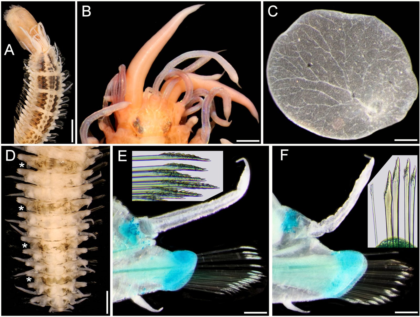
Figure 1. Lepidasthenia elegans (Grube, 1840), non-type specimens (USNM 47901). A, Largest specimen, anterior region, dorsal view; B, second largest specimen, anterior end, dorsal view; C, same, right elytron 2, seen from above; D, largest specimen, posterior region, dorsal view (*: elytra); E, same, chaetiger 10, left parapodium, anterior view (inset: tips of median neurochaetae); F, chaetiger 40, left parapodium, anterior view (inset: superior neurochaetae). Scale bars: A, 3 mm; B, 0.6 mm; C, 0.2 mm; D, 1.1 mm; E, F, 0.3 mm.
Description. Largest non-type specimen (USNM 47901) with body depressed, twisted; dorsum with 3 black longitudinal wide bands progressively paler, forming distinct blocks separated by a white segment, median band narrowest, often discontinuous (Fig. 1A); first block along chaetigers 2-7, then one segment pale, continued with blocks made of 3-4 segments, interrupted by a single pale segment, such that there are 4 blocks of 3 pigmented segments, followed by one with 4 segments, and then median and posterior regions with elytrigerous segments darker, followed by 2 paler cirrigerous segments. Venter pale, blackish along base of parapodia. Cephalic appendages and dorsal cirri white; elytra transparent. Pharynx fully exposed, brownish, 11 pairs of terminal papillae, transparent, some with a blackish core; 2 midlateral round papillae, behind terminal ones. Second largest specimen with pharynx not exposed; anterior elytra, and left parapodia of chaetigers 10 and 40 removed for observation (kept in container).
Prostomium bilobed, sub-hexagonal, slightly wider than long, facial tubercle not visible dorsally, globose. Eyes black, anterior eyes about 2 times as large as posterior ones, in widest prostomial area, directed laterally; posterior eyes close to posterior margin (Fig. 1B); in 3 specimens eyes enlarged, almost fused laterally. Median antenna slightly longer than right lateral one (left one in regeneration), ceratophore slightly wider than laterals; lateral antennae on prostomial anterior extensions; all ceratostyles cylindrical, mucronate. Palps massive, non-papillate, almost as long as median antenna, mucronate.
Tentacular segment not visible dorsally: tentaculophores long, cirrostyles wide, 3-4 times as long as prostomium; without chaetae. Segment 2 without nuchal lappet; first pair of parapodia and elytrophores directed anteriorly; ventral cirri 5-6 times as long as following ones (3-4 times in smallest specimen); elytrophores short anteriorly, minute along median and posterior rergions.
Elytra 30 pairs (22 in smallest specimen), smooth, without fimbriae, progressively smaller in median and posterior chaetigers; first 13(11) pairs alternating with cirrigerous segments, then present every third segment. First elytra with distinct branching venation from insertion area (Fig. 1C), posterior elytra minute slightly larger than elytrophore (Fig. 1D).
Parapodia sequiramous. Dorsal cirri with cirrophore short, cylindrical along anterior chaetigers, inserted basally (Fig. 1E), truncate conical in posterior chaetigers (Fig. 1F), terete, mucronate, surpassing neurochaetal tips. Notopodium short, round, without chaetae. Neuropodium with pre- and postchaetal lobes of similar size, both with margins smooth, without acicular lobes. Ventral cirri tapered, short, inserted basally. Nephridial lobes from segment 12, digitate.
Anterior chaetigers with neurochaetae barely swollen subdistally (Fig. 1E), pectinate area with petaloid spines, tips bidentate, accessory tooth almost as large as main one (Fig. 1E, inset). Posterior chaetigers with neurochaetae less spinous, of 3 types, superior neurochaetae thin, spinous superior giant neurochaetae darker with tips bidentate or unidentate, and thinner bidentate neurochaetae (Fig. 1F, inset).
Posterior region tapered; pygidium with anus terminal, with 2 small, lateral anal cirri (Fig. 1D.
Variation. Pigmentation pattern fades off in older specimens. Anterior eyes are usually 2 times as large as posterior ones, but they are laterally nearly fused in some specimens, but not in all. The sequence of elytrigerous and cirrigerous segments is constant; first 11-13 elytra alternate with cirri, following ones are in a sequence with one elytron and 2 dorsal cirri, to end of body.
Taxonomic summary
Type material. Polynoe elegans Grube, 1840; 2 syntypes (ZMB 17) from Sicily, 4 syntypes (ZMB 1176) from Palermo, and 2 syntypes (ZMB 1177) from unspecified Mediterranean localities, plus several other specimens in the same museum (Lesina: ZMB 1172; Luisin piccolo: 1173; and Cherso: 1174, 1175); pigmentation faded off.
Additional material. Three specimens (USNM 5144), Bay of Naples, Italy, 1893, purchased from Stazione Zoologica, Napoli (complete, barely pigmented, better defined in smallest specimen; some parapodia and elytra previously removed (kept in container); eyes better defined in one specimen, anterior eyes about 2 times as large as posterior ones; body 37-80 mm long, 4.5-8.5 mm wide, 65-82 chaetigers). Five specimens (USNM 47900), The Maire, Marseille, France, rocky bottom, 9 Apr. 1971, H. Zibrowius, coll. (3 complete; dorsal pigmentation pattern blackish to brownish, one with pharynx partially exposed, with 4 additional papillae, 2 basal to terminal ones, 2 others irregular; chaetigers 2-7 forming a continuous block, then blocks of mostly 3 segments interrupted by a pale segment anteriorly; one with diffuse pigmentation along medial and posterior regions, 2 others with elytrigerous segments darker than paler cirrigerous ones; anterior eyes 2 times as large as posterior ones, not fused laterally; posterior segments of larger specimens with a white mass inside basal dorsal cirri; body 50-70 mm long, 7.0-7.5 mm wide, 85-94 chaetigers). Four specimens (USNM 47901), Cap l’Abeille. 2 km south of Banyuls, France, corals, 30 m, 6 May 1967, M.H. Pettibone and L. Laubier, coll. (3 complete; body 27.5-50.5 mm long, 4.5-6.5 mm wide, 57-72 chaetigers; used for redescription).
Distribution. Mediterranean Sea, in shallow water coralligenous or rocky bottoms.
Remarks
Hartwich (1993: 96) listed several lots in Berlin and regarded them almost all as syntypes. After the study of many types of species described by Grube, we anticipate his type and non-type specimens should be colorless by now, and this explains why we selected one specimen with bright pigmentation for redescribing the species. The pigmentation pattern was clearly illustrated by Benham (1901: 293), and this is rather consistent in specimens from the Mediterranean Sea. Lepidasthenia elegans (Grube, 1840) has been reported from the Indian Ocean (Day, 1967; Potts, 1910), but those specimens differ in several features from the Mediterranean ones, such as the position of the anterior eyes, the type of dorsal and ventral cirri, and the shape of the giant neurochaetae. These records might belong in L. nuda (Grube, 1870), redescribed by Wehe (2006: 73), which could include L. affinis Horst, 1917.
Hartman (1959: 99) regarded Polynoe blainvillii Audouin & Milne Edwards, 1834 as a synonym of L. elegans (Grube, 1840). However, this publication is the compilation of some earlier publications, and the original proposal was P. blainvillii Audouin & Milne Edwards, 1832. Audouin and Milne-Edwards (1832: 430-431; 1834: 94-95) proposed the new name for a specimen briefly described and illustrated by de Blainville (1828: 459, Pl. 10, Fig. 2), but without locality, and identified as Eumolpe scolopendrina Savigny, 1822. The French specialists noted the differences with P. scolopendrina Savigny, 1822 such as having reduced elytra to the posterior end (larger, but missing in posterior region in P. scolopendrina). Regretfully, probably because it was identified as an already known species, de Blainville provided no morphological details in the description but in his illustrations (2: whole body, dorsal view; 2a: parapodium) the parapodium was depicted with notochaetae. As indicated above, notochaetae are missing in Lepidasthenia species, and if P. blainvillii is a Lepidasthenia, this could be an erroneous observation. The de Blainville specimen was not deposited, such that there is no means to clarify this potential synonymy.
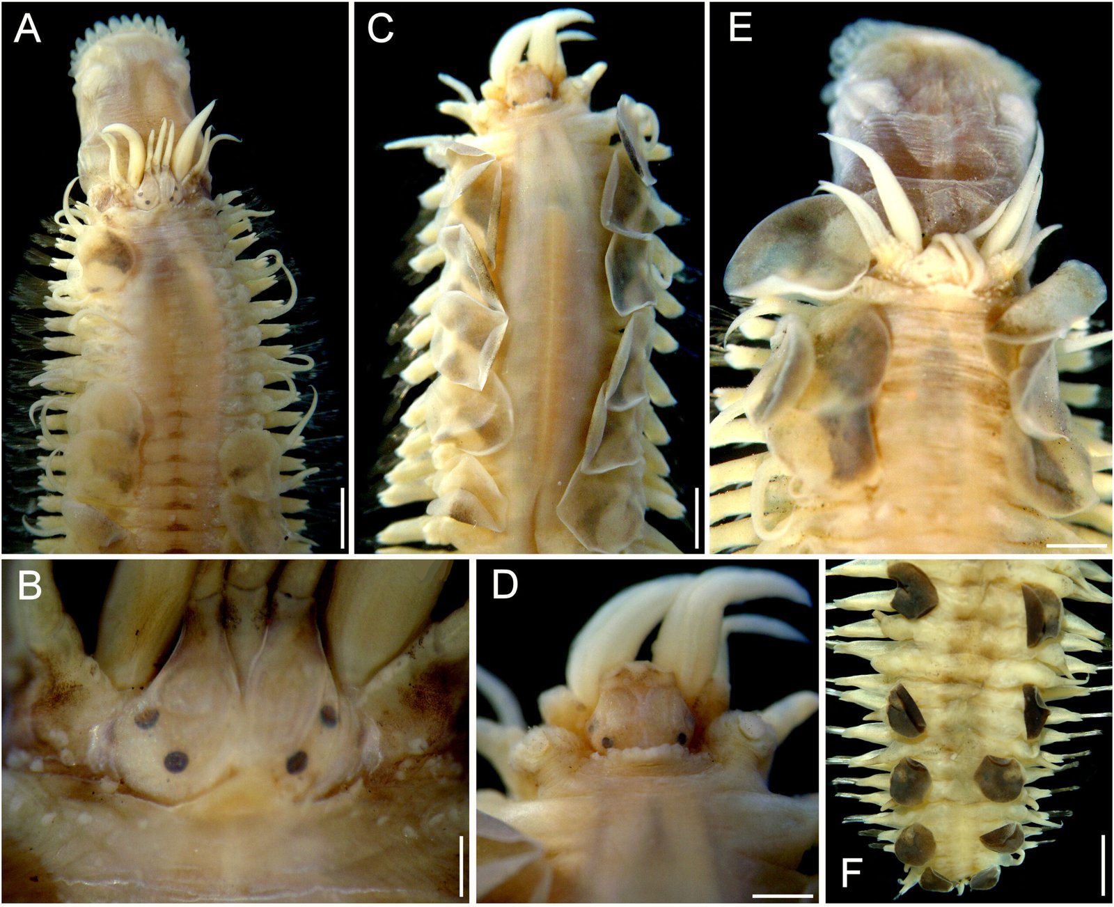
Figure 2. Lepidasthenia digueti Gravier, 1905, reinstated, syntypes (MNHN POLY TYPE). A, syntype 119, anterior region, dorsal view; B, same, close-up of anterior end; C, syntype MNHN POLY TYPE 120, anterior region, dorsal view; D, same, close-up of anterior end; E, syntype 119b, anterior region, dorsal view; F, same, posterior region, dorsal view. Scale bars: A, 1.5 mm; B, 0.1 mm; C, 1.7 mm; D, 0.7 mm; E, 1 mm; F, 1.3 mm.
Nevertheless, if P. scolopendrina sensu de Blainville, or P. blainvilli are ever recorded, they should not be retained as senior synonyms of P. elegans Grube, 1840. If they are found, it might be better to regard P. blainvilli as a nomen oblitum, and P. elegans would be a nomen protectum (ICZN 1999, Art. 23.9).
Lepidasthenia digueti Gravier, 1905, reinstated
Lepidasthenia digueti Gravier, 1905a: 177-181; 1905c: 160-173, Textfigs 1-9; Fauvel, 1943: 4-5; Salazar-Silva, 2006: 150.
Diagnosis. Lepidasthenia with nuchal lappet crenate: median and posterior elytra slightly smaller than anterior ones, brown to blackish, non-transparent; neurochaetae unidentate, without giant chaetae.
Description. Syntypes (MNHN POLY TYPE 119, 120; USNM 51613) in poor condition, fragmented, with grayish pigmentation on ceratophores, tentaculophores and on elytral surface (Fig. 2A, C, E), anterior pigmentation faded off in another syntype (USNM 51613) (Fig. 3A); body with small blackish spots dorsally on anterior segments, darker along posterior segments.
Prostomium bilobed, wider than long; facial tubercle reduced. Two pairs of eyes, dark, rounded, of similar size, anterior eyes on widest prostomial area, dorsolateral, posterior eyes dorsal, near posterior prostomial margin (Figs. 2B, D, 3B). Median antenna with ceratophore thin, short, grayish, inserted frontally between prostomial lobes, ceratostyle thick, long, tapering in filiform tip, slightly longer than lateral ceratostyles. Lateral antennae with ceratophores thick, short, grayish, inserted terminally, ceratostyles thinner, long, taper in filiform tip. Palps thin, pale, long, tapered, tip filiform, surface smooth, non-papillate. Pharynx fully exposed in one syntype (MNHN POLY TYPE 119) (Fig. 2A), brownish, with 14 pairs of terminal papillae, and 2 subdistal lateral low tubercles.
Tentacular segment not visible dorsally. Tentaculophores, thick, short, without chaetae, not covered by elytrophores, tentacular cirri long, as long as antennae but thinner. Second segment projected on prostomium as a short nuchal lobe, margin crenate. First pair of elytrophores not expanded dorsally, with some scattered papillae.
Numerous elytra (number indeterminate due to condition of specimens); first elytra present in one syntype (Fig. 2E), slightly larger than following ones, apparently not completely covering anterior end; after pair 12 alternate with 2 dorsal cirri, on the posterior segments elytra alternate with 2 or 3 dorsal cirri. Elytra small, not overlapped middorsal, covering 2 adjacent segments. Elytral margins smooth, without fimbriae; anterior elytra surface with brown area diffuse mainly toward mid-dorsal line, posterior elytra with homogeneous pigmentation.
Parapodia biramous. Notopodia reduced to small lobes. Neuropodia long, thin, with prechaetal and postchaetal lobes rounded, of similar size. Dorsal tubercles absent, elytrophores small, rounded, not directed dorally. Dorsal cirri pale, smooth, cirrophores short, slightly swollen. Ventral cirri long, thick, tapered in filiform tip, cirrophore short, thick. Anterior segments with neuropodia with 3-4 fungiform ventral papilla (Fig. 3D); median and posterior chaetigers with neuropodia ventrally smooth (Fig. 3E). Nephridial papillae from segment 10.
Notochaetae absent. Neurochaetae with pectinate area variably modified along bundle; anterior chaetigers with lower neurochaetae with longer pectinate area (Fig. 3D, inset); median and posterior chaetigers with neurochaetal pectinate area decreasing in size ventrally (Fig. 3E, inset); pectinate area with series of long, petaloid spines; tips bidentate, main tooth short, accessory denticle shorter, almost completely fused to main tooth. No giant neurochaetae present.
Posterior region tapered (Figs 2F, 3F); pygidium with anus terminal, anal cirri short, ventral.
Taxonomic summary
Type material. Syntypes of Lepidasthenia digueti Gravier, 1905 (MNHN POLY TYPE 119, 120; USNM 51613), La Paz, Baja California, Gulf of California, México, 1904, L. Diguet, coll.
Distribution. Only known from the Gulf of California, associated with an unidentified, intertidal balanoglossid hemichordate.
Remarks
Lepidasthenia digueti Gravier, 1905 is easily recognized as belonging to Lepidasthenia since the original description after the sequence of elytra in posterior segments being present every third segment, the lack of notochaetae, and the elongate neuropodial lobes. This is confirmed despite the fragmented condition of the type specimens. The crenate nuchal hood is very distinctive, although this was not included in the original description, together with the sequence of elytra and cirri along median segments.
The syntype specimens are all fragments, as originally indicated by Gravier (1905a: 179, 1905c: 163), but they include both body ends, and their features correspond to Lepidasthenia. After the type of sequence of elytra-dorsal cirri along median and posterior regions, and after the presence of apparently unidentate neurochaetae (accessory denticle minute), we confirm it belonging in Lepidasthenia. Lepidasthenia digueti belongs in the group of species having apparently unidentate neurochaetae, without giant chaetae, and without ventral papillae along neuropodial surface.
Solís-Weiss et al. (2004: S14) hesitated about the type status of the Paris Museum specimens, probably because they were fragments; we confirm the 2 Paris specimens and the one in Washington are all syntypes. It is enigmatic, however, how a syntype was sent to Washington; there are no indications in the catalogue card for the specimen about how it reached Washington, and it is likely that Dr. Marian Pettibone, after her long-time involvement with polynoid polychaetes, received it as a donation from the Paris museum.
Read and Fauchald (2024a) have listed L. digueti in Lepidametria after Seidler (1923). This confusion has 2 explanations. First, Gravier (1905a: 180; 1905b: 166) indicated there was a non-exposed notopodial compact bundle of chaetae, but after the study of type specimens, Fauvel (1943: 4) explained they were fibers inserted close to acicular tips, and confirmed L. digueti was a true Lepidasthenia after the lack of notochaetae, but this conclusion was overlooked. Second, Seidler (1923: 258) studied one specimen from Charlestown, and he indicated the locality was in the Pacific coast of Central America. This is wrong. Charlestown is the capital of Nevis Island, in the archipelago of Saint-Kitts and Nevis, in the Caribbean Sea. His specimen might belong to a likely undescribed, western Atlantic species of Lepidametria.We think it is incorrect to incorporate an eastern Pacific species from one genus, into any other on the basis of specimens from a very different ocean basin, or without the study of type material.
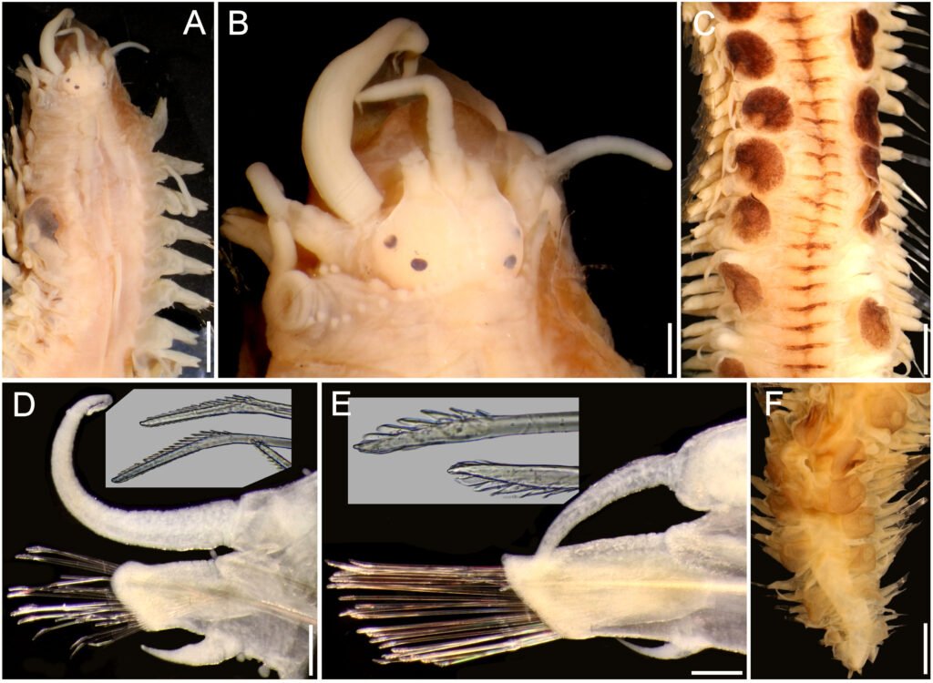
Figure 3. Lepidasthenia digueti Gravier, 1905, reinstated, syntype (USNM 51613). A, Anterior region, dorsal view, first right parapodia previously removed; B, anterior end, dorsal view; C, median fragments, dorsal view; D, anterior chaetiger, right parapodium, anterior view (inset: lower neurochaetae tips); E, median chaetiger, right parapodium, anterior view (inset: median neurochaetae tips); F, posterior region, dorsal view. Scale bars: A, 1.3 mm; B, 0.4 mm; C, F, 1.6 mm; D, E, 0.3 mm.
The hemichordate was not described soon, as indicated by Gravier (1905a, c), and its identity remains unknown. The hemichordate could be Ptychodera flava Eschscholtz, 1825, a widely distributed species in the Indian and Pacific oceans (Uribe & Larrain, 1992).
Lepidonotinae Willey, 1902
Lepidametria Webster, 1879
Type species. Lepidametria commensalis Webster, 1879, by monotypy.
Diagnosis (after Salazar-Vallejo et al., 2015). Lepidonotinae with a long body with up to 80 segments. Elytrae large, covering body or leaving a narrow dorsal surface uncovered; posterior region with elytra and cirri alternating every other segment. Tentaculophores with chaetae. Notopodia reduced, with fine notochaetae at least along anterior and median segments, rarely absent. Neuropodia projecting with several types of neurochaetae. Ventral surface often papillated.
Remarks
As indicated by Pettibone (1953) and Salazar-Vallejo et al. (2015), Lepidametria differs from Lepidasthenia because it has notochaetae, and alternating elytra and cirri along median and posterior segments, whereas in Lepidasthenia there are no notochaetae, and elytra occur every third segment. The need for a redescription of the type material was indicated elsewhere (Salazar-Vallejo et al. 2015: 26). In a recent contribution (Salazar-Vallejo et al. 2015) we regarded Bouchiria Wesenberg-Lund, 1949, as a junior synonym of Lepidametria; it is a junior synonym but of Lepidasthenia, as indicated by Wehe (2006).
Read and Fauchald (2024) list 4 species in Lepidametria: L. brunnea Knox, 1960; L. commensalis, L. digueti (Gravier, 1905); and L. lactea (Treadwell, 1939). We have shown above that L. digueti belongs in Lepidasthenia, we regard L. brunnea as belonging in Lepidasthenia because it lacks notochaetae, and has elytra every 3 segments along posterior region, and we confirm Hartman (1951) synonymy of L. lactea with L. commensalis. Consequently, there would only be one species in Lepidametria (L. commensalis); however, we think that L. virens (Blanchard in Gay, 1849), and L. gigas (Johnson, 1897) also belong in this genus. A key to species is included below.
Lepidametria commensalis Webster, 1879
Figs. 4, 5
Lepidametria commensalis Webster, 1879: 209-212, Pl. 3, Figs. 23-31; Hartman, 1951: 17 (syn.); Pettibone, 1963: 19-20, Fig. 4k; Day, 1973: 6; Gardiner, 1976: 86-87, Fig. 1k-n.
Lepidasthenia lactea Treadwell, 1939: 3-5, Figs. 13-15.
Diagnosis. Lepidametria with nuchal lappet smooth: median and posterior elytra slightly smaller than anterior ones, with dark spots, non-transparent; neurochaetae uni- and bidentate, with giant chaetae in median chaetigers.
Description. Syntypes of Lepidametria comensalis (USNM 527) include one beheaded specimen, better preserved (probably used for original description), and a complete specimen; description based on the complete soft syntype. Some parapodia and elytra already dissected (kept in container); no further dissections to avoid additional damage.
Body long, depressed, variably damaged, 70 mm long, 6 mm wide, 71 segments, dorsum with diffuse brownish intersegmental bands (Fig. 4A) [paratype of L. lactea (USNM 20420) 20 mm long, 64 segments; holotype of L. lactea (AMNH 2565) with 50 mm long, 2 mm wide, 62 segments, 34 pairs of elytra].
Prostomium bilobed, longer than wide, without facial tubercle (Fig. 4B). Eyes blackish, visible dorsally, small; anterior eyes in widest prostomial area. Median antenna lost, ceratophore cylindrical, long. Lateral antennae lost, on prostomial anterior extensions, ceratophores as long as median one. Palps massive, long, with papillae, tapered into fine tips.
Tentacular segment not visible dorsally; tentaculophores long, cirrostyles wide, 2 times as long as prostomium. Segment 2 with nuchal lappet; first pairs of parapodia and elytrophores perpendicular, not directed anteriorly; ventral cirri about 2 times as long as following ones. Without dorsal tubercles; elytrophores short.
Elytra 44 pairs, subcircular, thin, transparent, smooth, without fimbriae (Fig. 4C), non-overlapping mid-dorsally, except posterior pair; after pair 12, most alternating with dorsal cirri; elytra pairs 12 and 13, and 14 and 15 contiguous (no dorsal cirri between them). Posterior region with elytra paired along 3-4 segments, then one elytrigerous, followed by one or 2-3 pairs of elytra.
Parapodia biramous, short, about as long as half body width (Fig. 4D). Dorsal cirri thick, short, not surpassing neuropodial tips, subdistally swollen, with long tips, with a brown band in widened area; cirrophore thick, short, swollen basally, inserted basally. Notopodia with notochaetae present along body, missing in far posterior chaetigers. Neuropodia with pre- and postchaetal lobes of similar size, prechaetal lobe lobulate along superior part, continuous along lower part, postchaetal lobe continuous, without acicular lobes. Ventral cirri short, thin, inserted medially in neuropodium. Nephridial lobes cylindrical, long, from segment 8.
Notochaetae scarce, smooth capillaries, not reaching neuropodial tips (Fig. 4D, inset). Neurochaetae most bidentate, a few unidentate, pectinate area slightly wider, rows of spines restricted to wider basal area. Median segments with a single giant unidentate neurochaeta, denticles minute (Fig. 4E, inset).
Posterior end tapered; anus terminal, anal cirri thin.
Variation. A smaller specimen (USNM 52842), mature female, has elytra overlapping completely along middorsum (Fig. 5A), transverse intersegmental bands visible. Prostomium pale, with ceratophores brownish (Fig. 5B); median antenna about 2 times as long as both prostomium and lateral antennae (left one in regeneration), ceratostyles barely swollen, darker than adjacent areas; palps thick, papillate, about 2 times as long as median antenna. Tentaculophores with cirrostyles slightly shorter than median antenna, right one with a single chaeta. Second segment with nuchal lappet.
Elytra oval, wider than long, with brown spots, including insertion areas (Fig. 5C). In posterior chaetigers, elytral sequence is 3 elytrigerous followed by one cirrigerous and then 3 other elytrigerous (Fig. 5D). Dorsal tubercles distinct in cirrigerous segments, at least along posterior region.
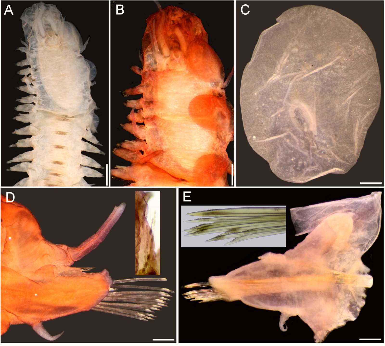
Figure 4. Lepidametria commensalis Webster, 1879, complete syntype (USNM 527). A, Anterior region, dorsal view; B, anterior end, dorsal view, after Shirlastain-A; C, elytron from unknown chaetiger, seen from above; D, cirrigerous parapodium from an unknown chaetiger, dorsal cirrus broken, after Shirlastain-A (inset: close-up of notochaetae); E, elytrigerous parapodium from an unknown chaetiger, elytron folded backwards, after Shirlastain-A (inset: neurochaetae). Scale bars: A, 1.3 mm; B, 1 mm; C-E, 0.3 mm.
Cirrigerous parapodia with dorsal cirri barely swollen subdistally, with brown band, with more abundant notochaetae along anterior region (Fig. 5E), neurochaetae of similar width; posterior parapodia with less notochaetae, and upper giant spine; neurochaetae mostly bidentate, progressively unidentate dorsally (Fig. 5F, inset). Oocytes about 100 µm in diameter.
Two other specimens, complete (USNM 52840, 52841) have elytra overlapping laterally, but leaving a narrow middorsal area uncovered; dorsum with complex pigmentation pattern: the transverse bands are clearly on the posterior part of each segment, not intersegmental, and there is a wide, oval brownish spot along most dorsal surface of each segment, although it can be interrupted medially by a paler area. One specimen (USNM 52841) with pharynx partially exposed, jaws are brownish, and there are 10 upper and 11 lower terminal papillae. Giant neurochaetae from second third of body (chaetigers 23 of 71; 25 of 70 in USNM 52840). One specimen (USNM 52840) with nephridial lobes globose, truncate, from chaetiger 8. Posterior region tapered, anus terminal, anal cirri resembling dorsal cirri.
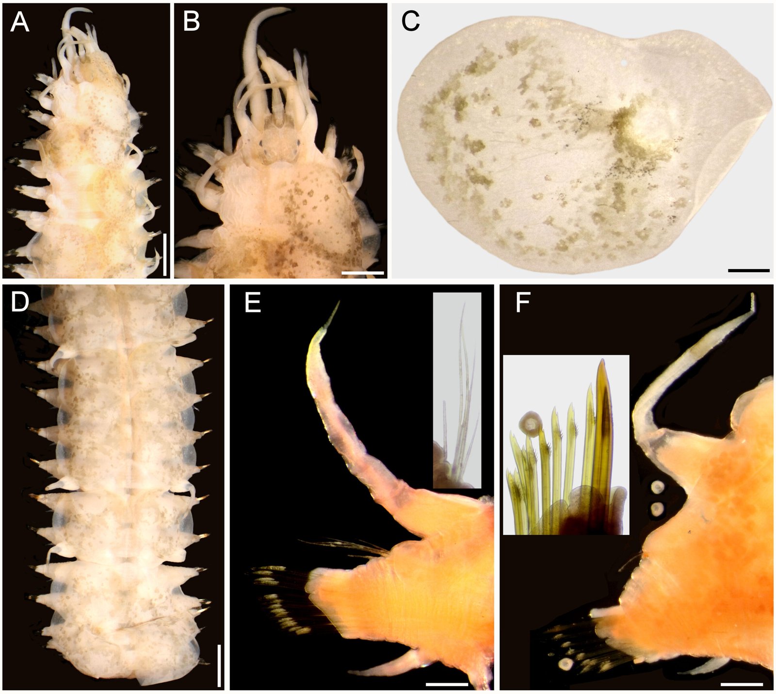
Figure 5. Lepidametria commensalis Webster, 1879, non-type specimen (USNM 52842). A, Anterior region, dorsal view; B, anterior end, dorsal view; C, elytron 3 right, seen from above; D, posterior region, dorsal view; E, chaetiger 10, right parapodium, anterior view, after Shirlastain-A (inset: notochaetae); F, chaetiger 45, right parapodium, anterior view, after Shirlastain-A (inset: neurochaetae). Scale bars: A, 1.4 mm; B, 0.8 mm; C, E, F, 0.3 mm; D, 1.2 mm.
Another specimen (USNM 56533) rolled ventrally, elytra almost completely brownish, with pale spots in insertion area; posterior segments have 3 elytra in sequence.
Taxonomic summary
Type material. Two syntypes of Lepidametria commensalis (USNM 527), Virginia, USA, Sta. H458, H. E. Webster, coll. Holotype of Lepidasthenia lactea (AMNH 2565), Galveston, Texas, USA Paratype of L. lactea (USNM 20420), Galveston, Texas, USA, O. Sanders, coll.
Additional material. One specimen (USNM 52840), Banks Channel, Wrightsville Beach, North Carolina, intertidal, in Amphitrite ornata tube, Mar. 1973, S.L. Gardiner, coll. (complete, bent laterally, pharynx partially exposed; body 70 mm long, 5 mm wide, chaetigers). One specimen (USNM 52841), Banks Channel, Wrightsville Beach, North Carolina, intertidal, in Amphitrite ornata tube, 8 Mar. 1974, S.L. Gardiner, coll. (pigmentation pattern indicated in variation; body 50 mm long, 4.5 mm wide, 71 chaetigers). One specimen (USNM 52842), mature female, without posterior end, intracoastal waterway, Wrightsville Beach, North Carolina, intertidal, in Amphitrite ornata tube, 5 Apr. 1974, T. Fox, coll. (pale, with elytra mottled; right elytra 1 and 3, and right parapodia of chaetigers 10 and 45 removed for observation (kept in container); body 66 mm long, 5 mm wide, 66 chaetigers). One specimen (USNM 56533), York River, Virginia, 29 Jul. 1977 (markedly bent ventrally, 2 posterior parapodia and many elytra detached (30 elytra and 2 parapodia in container); not measured for avoiding further damage).
Distribution. Virginia to Texas, USA, in shallow waters, associated with terebellid polychaetes, and with sponges (Dauer 1973).
Remarks
Webster (1879: 211) indicated that the sequence of elytra and cirri was asymmetrical in posterior chaetigers, such that one elytron could be on side, and one dorsal cirri on the other side. This was confirmed in the beheaded syntype, but this is not present in the other non-type specimens. Bergström (1916) noted this same anomaly in other long-bodied polynoids, and it has been recently reported for another species (Salazar-Vallejo, 2024).
Hartman (1951) regarded Lepidasthenia lactea Treadwell, 1939 as a junior synonym of L. commensalis Webster, 1879. The type specimens of L. lactea have a similar shape of prostomium, and share the same type of elytra, noto- and neurochaetae, but they are smaller, such that the specimens might be juveniles.
Webster (1879) found L. commensalis living in tubes of the terebellid Amphitrite ornata (Leidy, 1855), and Hartman (1951) found it living with Thelepus setosus (de Quatrefages, 1866), whereas L. lactea was found in different, unidentified terebellid tubes.
Key to species of Lepidametria Webster, 1879
1 Median and posterior elytra regularly alternating with dorsal cirri …………………… 2
– Median and posterior elytra not regularly alternating …………………… L. virens (Blanchard in Gay, 1849) Chile
2(1) Elytra present along body …………………… L. commensalis Webster, 1879 Northwestern Atlantic
– Elytra not reaching posterior end …………………… L. gigas (Johnson, 1897) California
Acknowledgments
The generous support by curators and collection managers is deeply acknowledged. Karen Osborn and Karen Reed currently, Linda Ward, the late Kristian Fauchald, formerly (USNM), Fredrik Pleijel and Tarik Meziane (MNHN). They all were and have been very supportive of our research activities and provided lab space and facilities for this study. Anabel León-Hernández and Daniel Pech provided some publications. The careful reading by two anonymous referees helped us to improve this final contribution. In her usual high standards, María Antonieta Arizmendi kindly took care of all the formatting issues for this publication.
References
Amaral, A. C., & Nonato, E. F. (1982). Anelideos poliquetos da costa brasileira. Aphroditidae e Polynoidae. Brasilia: Conselho Nacional de Desenvolvimento Científico e Tecnológico.
Audouin, J. V., & Milne-Edwards, H. (1832). Classification des annélides, et description de celles qui habitent les côtes de la France. Annales des Sciences Naturelles, 27, 337–447.
Audouin, J. V., & Milne-Edwards, H. (1834). Recherches pour servir à l’histoire naturelle du littoral de la France, ou recueil de mémoires sur l’anatomie, la physiologie, la classification et les mœurs des animaux de nos côtes (Vol. 2, Pt. 1). Paris: Crochard.
Barnich, R., & Fiege, D. (2003). The Aphroditoidea (Annelida: Polychaeta) of the Mediterranean Sea. Abhandlungen der Senckenbergischen Naturforschenden Gesellschaft, 559, 1–170.
Barnich, R., & Fiege, D. (2004). Revision of the genus Lepidastheniella Monro, 1924 (Polychaeta: Polynoidae: Lepidastheniinae) with notes on the subfamily Lepidastheniinae and the description of a new species. Journal of Natural History, 38, 863–876. https://doi.org/10.1080/0022293021000046432
Benham, W. B. (1901). Polychaet worms. In S. F. Harmer & A. E. Shipley (Eds.), The Cambridge natural history (Vol. 2). London: Macmillan.
Bergström, E. (1916). Die Polynoiden der schwedischen Sudpolarexpedition 1901-1903. Zoologiska Bidrag från Uppsala, 4, 269–304.
Brown, R. W. (1954). Scientific words: a manual of methods and a lexicon of materials for the practice of logotechnics. Baltimore: George W. King.
Chamberlin, R. V. (1919). The Annelida Polychaeta [Albatross Expeditions]. Memoirs of the Museum of Comparative Zoology at Harvard College, 48, 1–514.
Dauer, D. M. (1973). Polychaete fauna associated with Gulf of Mexico sponges. Florida Scientist, 36, 193–196.
Day, J. H. (1967). A monograph on the Polychaeta of South Africa. Part 1. Errantia (Vol. 656). London: British Museum (Natural History).
Day, J. H. (1973). New Polychaeta from Beaufort, with a key to all species recorded from North Carolina. NOAA Technical Report, National Marine Fisheries Services Circular, 375, 1–153.
De Blainville, H. M. D. (1828). Vers. Dictionnaire des Sciences Naturelles, 57, 365–625. https://www.biodiversitylibrary.org/page/25316888 [Atlas: https://www.biodiversitylibrary.org/page/24394694]
De Quatrefages, A. (1866). Histoire naturelle des Annelés marins et d‘eau douce. Annélides et Géphyriens (Vol. 2). Paris: Librairie Encyclopédique de Roret.
Eschscholtz, F. (1825). Berich über die zoologisch Ausbeute der Reise von Kronstadt bis St. Peter und Paul. Isis von Oken, 1825.
Fauvel, P. (1917). Annélides polychètes de l’Australie méridionale. Archives de Zoologie Expérimentale et Générale, 56, 159–277. https://www.biodiversitylibrary.org/page/6322379
Fauvel, P. (1923). Polychètes errantes. Paris: Fédération Française des Sociétés de Sciences Naturelles.
Fauvel, P. (1943). Annélides polychètes de Californie. Mémoires du Muséum National d’Histoire Naturelle, nouvelle série, 18, 1–32. https://www.biodiversitylibrary.org/page/59784292
Gardiner, S. L. (1976). Errant polychaete annelids from North Carolina. Journal of the Elisha Mitchell Scientific Society, 91, 78–220.
Gay, C. (1849). Historia física y política de Chile, según documentos adquiridos en esta república durante doce años de residencia en ella. Zoología, Tomo 3, 9–52; Atlas 2, Pls. 1-3. Santiago: Museo de Historia Natural. https://www.biodiversitylibrary.org/page/16438163 [Atlas: https://www.biodiversitylibrary.org/page/55213605]
Gravier, C. (1905a). Sur un Polynoidien (Lepidasthenia digueti nov. sp.) commensal d’un Balanoglosse de Basse-Californie. Bulletin du Muséum d’Histoire Naturelle, Paris, 11, 177–184.
Gravier, C. (1905b). Sur les genres Lepidasthenia Malmgren et Lepidametria Webster. Bulletin du Muséum d’Histoire Naturelle, Paris, 11, 181–184.
Gravier, C. (1905c). Sur un polynoïden (Lepidasthenia digueti nov. sp.), commensal d’un balanoglosse de Basse-Californie. Bulletin de la Société Philomatique de Paris, neuvième série, 7, 160–173.
Grube, A. E. (1840). Actinien, Echinodermen und Würmer des Adriatischen- und Mittelmeers nach eigenen Sammlungen beschrieben. J.H. Bon, Königsberg. https://www.biodiversitylibrary.org/page/10662919
Grube, E. (1870). Bemerkungen über anneliden des Pariser Museums. Archiv für Naturgeschichte, Berlin, 36, 281–352.
Hartman, O. (1942). A review of the types of polychaetous annelids at the Peabody Museum of Natural History, Yale University. Bulletin of the Bingham Oceanographic Collection, Yale University, 8, 1–98.
Hartman, O. (1951). The littoral marine annelids of the Gulf of Mexico. Publications of the Institute of Marine Science, Port Aransas, Texas, 2, 7–124.
Hartman, O. (1959). Catalogue of the polychaetous annelids of the world (Occasional paper No. 23). Los Angeles: Allan Hancock Foundation Publications.
Hartwich, G. (1993). Die Polychaeten-Typen des Zoologischen Museums in Berlin. Mitteilungen aus der Zoologischen Sammlung des Museums für Naturkunde in Berlin, 69, 73–154.
Horst, R. R. (1917). Polychaeta Errantia of the Siboga Expedition. Part Ii Aphroditidae and Chrysopetalidae. Siboga Expeditie, 24, 46–143.
Imajima, M., & Hartman, O. (1964). The polychaetous annelids of Japan (Occasional paper No. 26). Los Angeles: Allan Hancock Foundation.
International Commission on Zoological Nomenclature (ICZN). (1999). International Code of Zoological Nomenclature. Natural History Museum. https://code.iczn.org
Johnson, H. P. (1897). A preliminary account of the marine annelids of the Pacific Coast, with descriptions of new species. Proceedings of the California Academy of Sciences, 1, 153–194.
Kinberg, J. G. H. (1856). Nya slägten och arter af Annelider. Öfversigt af Kongl. Vetenskaps-Akademiens Förhandlingar Stockholm, 12, 381–388.
Knox, G. A. (1960). Biological results of the Chatham Islands 1954 Expedition. Part 3. Polychaeta errantia. New Zealand Department of Scientific and Industrial Research Bulletin, 139, 77–143.
Leidy, J. (1855). Contributions towards a knowledge of the marine invertebrate fauna of the coasts of Rhode Island and New Jersey. Journal of the Academy of Natural Sciences of Philadelphia, 3, 135–152.
Malmgren, A. J. (1867). Annulata Polychaeta Spetsbergiæ, Grœnlandiæ, Islandiæ et Scandinaviæ. Hactenus cognita. Helsingforsiae, Ex Officina Frenckelliana.
Núñez, J., Barnich, R., Brito, M. C., & Fiege, D. (2015). Familias Aphroditidae, Polynoidae, Aceotidae, Sigalionidae y Pholoidae. Fauna Ibérica, 41, 89–257.
Núñez, J., Brito, M. C., & Ocaña, O. (1992). A new species of Lepidasthenia (Polychaeta: Polynoidae) from Canary Islands. Zoologica Scripta, 21, 347–349. https://doi.org/10.1111/j.1463-6409.1992.tb00336.x
Pettibone, M. H. (1953). Some scale-bearing polychaetes of Puget Sound and adjacent waters. Seattle, WA: University of Washington Press.
Pettibone, M. H. (1963). Marine polychaete worms of the New England region, 1. Families Aphroditidae through Trochochaetidae. Bulletin of the United States National Museum, 227, 1–356.
Pettibone, M. H. (1970). Polychaeta Errantia of the Siboga Expedition. Part IV. Some additional polychaetes of the Polynoidae, Hesionidae, Nereidae, Goniadidae, Eunicidae, and Onuphidae, selected as new species by the late Dr. Hermann Augener with remarks on other related species. Siboga-Expeditie Uitkomsten op Zoologisch, Botanisch, Oceanographisch en Geologisch Gebied verzameld in Nederlandsch Oost-Indië 1899–1900. Siboga – Expedition, 24, 199–270.
Pettibone, M. H. (1989). A new species of Benhamipolynoe (Polychaeta: Polynoidae: Lepidastheniinae) from Australia, associated with the unattached stylasterid coral Conopora adeta. Proceedings of the Biological Society of Washington, 102, 300–304.
Potts, F. A. (1910). The Percy Sladen Trust Expedition to the Indian Ocean in 1905, under the leadership of Mr. J. Stanley Gardiner: 12. Polychaeta of the Indian Ocean, 2. The Palmyridae, Aphroditidae, Polynoidae, Acoetidae and Sigalionidae. Transactions of the Linnean Society of London, Series 2, Zoology, 16, 325–353.
Read, G., & Fauchald, K. (Eds.). (2024a). World polychaeta database. Lepidametria Webster, 1879. https://www.marinespecies.org/aphia.php?p=taxdetails&id=236705 (Retrieved on August 20th, 2024).
Read, G., & Fauchald, K. (Eds.). (2024b). World polychaeta database. Lepidasthenia Malmgren, 1867. https://www.marinespecies.org/aphia.php?p=taxdetails&id=129495 (Retrieved on August 20th, 2024).
Salazar-Silva, P. (2006). Scaleworms (Polychaeta: Polynoidae) from the Mexican Pacific and some other Eastern Pacific sites. Investigaciones Marinas, Valparaíso, 34, 143–161.
Salazar-Vallejo, S. I. (2024). Barnichia crialesae gen. nov., sp. nov., from the western Atlantic (Annelida, Polychaeta, Polynoidae, Polynoinae). Bulletin of Marine Science, 100, 439–449. https://doi.org/10.5343/bms.2023.0103
Salazar-Vallejo, S. I., González, N. E., & Salazar-Silva, P. (2015). Lepidasthenia loboi sp. n. from Puerto Madryn, Argentina (Polychaeta, Polynoidae). Zookeys, 546, 21–37. https://doi.org/10.3897/zookeys.546.6175
Savigny, J. C. (1822). Système des annélides, principalement de celles des côtes de l’Égypte, et de la Sirie, offrant les caractères tant distinctifs que naturels des Ordres, Familles et Genres, avec la description des Espèces. Description de l’Égypte, Tome 1. Paris.
Seidler, H. J. (1923). Über neue und wenig bekannte Polychäten. Zoologischer Anzeiger, 61, 254–264.
Seidler, H. J. (1924). Beiträge zur Kenntnis der Polynoiden 1. Archiv für Naturgeschichte, 89, 1–217.
Solís-Weiss, V., Bertrand, Y., Helléouet, M. N., & Pleijel, F. (2004). Types of polychaetous annelids at the Muséum national d’Histoire naturelle, Paris. Zoosystema, 26, 377–384.
Treadwell, A. L. (1937). The Templeton Crocker Expedition. 8. Polychaetous annelids from the west coast of Lower California, the Gulf of California and Clarion Island. Zoologica, Scientific Contributions of the New York Zoological Society, 22, 139–160.
Treadwell, A. L. (1939). New polychaetous annelids from New England, Texas and Puerto Rico. American Museum Novitates, 1023, 1–7.
Uribe, M. E., & Larraín, A. P. (1992). Estudios biológicos en el enteropneusto Ptychodera flava Eschscholtz, 1825 de Bahía Concepción, Chile. 1. Aspectos morfológicos y ecológicos. Gayana Zoología, 56, 141–180.
Von Marenzeller, E. (1874). Zur Kenntnis der adriatischen Anneliden. Sitzungsberichte der Kaiserlichen Akademie der Wissenschaften, Mathematisch-Naturwissenschaftliche Classe, 69, 407–482.
Von Marenzeller, E. (1876). Zur Kenntniss der adriatischen Anneliden. Zweiter Beitrag. (Polynoinen, Hesioneen, Syllideen). Sitzungsberichte der Kaiserlichen Akademie der Wissenschaften, Wien, Mathematisch-Naturwissenschaftliche Classe, 72, 129–171.
Webster, H. E. (1879). The Annelida Chaetopoda of the Virginian coast. Transactions of the Albany Institute, 9, 202–269.
Wehe, T. (2006). Revision of the scale worms (Polychaeta: Aphroditoidea) occurring in the seas surrounding the Arabian Peninsula. 1. Polynoidae. Fauna of Arabia, 22, 23–197.
Wesenberg-Lund, E. (1949). Polychaetes of the Iranian Gulf. Danish Scientific Investigations in Iran, 4, 247–400.
Willey, A. (1902). Polychaeta. In B. Sharpe, & J. Bell (Eds.), Report on the Collections of Natural History made in the Antarctic Regions during the Voyage of the “Southern Cross (pp. 262–283). London: British Museum.

Análisis de la diversidad y nuevos registrosde equinodermos (Echinodermata) para el Parque Nacional Revillagigedo, México
Ingrid Yutzil Ruiz-Nuñez a, Cristian M. Galván-Villa a, *, Omar Domínguez-Domínguez b, Rebeca Granja-Fernández a, c, Miriam Hueytletl-Pérez d y Francisco Alonso Solís-Marín e
a Universidad de Guadalajara, Centro Universitario de Ciencias Biológicas y Agropecuarias, Departamento de Ecología Aplicada, Laboratorio de Ecología, Conservación y Taxonomía, Camino Ramón Padilla Sánchez Núm. 2100, 45200 Zapopan, Jalisco, México
b Universidad Michoacana de San Nicolás de Hidalgo, Facultad de Biología, Laboratorio de Biología Acuática, Av. Francisco J. Múgica s/n, Ciudad Universitaria, 58030 Morelia, Michoacán, México
c Universidad de Guadalajara, Centro Universitario de Ciencias Biológicas y Agropecuarias, Investigación posdoctoral (SECIHTI)-Programa de Maestría en Biosistemática y Manejo de Recursos Naturales y Agrícolas, Camino Ramón Padilla Sánchez Núm. 2100, 45200 Zapopan, Jalisco, México
d Instituto Politécnico Nacional, Centro Interdisciplinario de Ciencias Marinas, Programa de Doctorado en Ciencias Marinas, Av. Instituto Politécnico Nacional s/n, Playa Palo de Santa Rita, 23096 La Paz, Baja California Sur, México
e Universidad Nacional Autónoma de México, Instituto de Ciencias del Mar y Limnología, Laboratorio de Sistemática y Ecología de Equinodermos, Circuito Exterior s/n, Ciudad Universitaria, Coyoacán, 04510 Ciudad de México, México
*Autor para correspondencia: cristian.galvan@academicos.udg.mx (C.M. Galván-Villa)
Resumen
Compuesto por 4 islas volcánicas tropicales, el archipiélago de Revillagigedo cuenta con ecosistemas únicos y bien preservados que lo han incluido en la lista de patrimonio mundial de la UNESCO. El objetivo de este trabajo fue dar a conocer un inventario actualizado de equinodermos del Parque Nacional Revillagigedo, incluidos registros nuevos de especies de las clases Asteroidea y Ophiuroidea, y un análisis de su composición. La diversidad de las islas se evaluó mediante análisis ecológicos (riqueza de especies, similitud y distintividad taxonómica). En total, se obtuvieron 94 especies de equinodermos de las cuales 5 son nuevos registros, 2 estrellas de mar (Heliaster kubiniji y Astrometis sertulifera) y 3 ofiuros (Ophiolepis variegata, Ophiopsila californica y Ophiothela mirabilis). La clase con mayor número de especies en todo el parque resultó ser Ophiuroidea con 31, seguida de Asteroidea, Echinoidea y Holothuroidea con 21 cada una. Las islas Clarión (60 spp.) y Socorro (58 spp.) presentaron la mayor riqueza de especies y diversidad taxonómica. Sin embargo, la riqueza de especies en San Benedicto y Roca Partida puede estar subestimada debido a un menor esfuerzo de muestreo histórico realizado en estas islas.
Palabras clave: Área natural protegida; Pacífico oriental; Similitud; Diversidad taxonómica; Islas oceánicas
Diversity analysis and new records of echinoderms (Echinodermata) for Revillagigedo National Park, Mexico
Abstract
Consisting of 4 tropical volcanic islands, the Revillagigedo Archipelago has unique and well-preserved ecosystems that have placed it on the UNESCO World Heritage List. The objective of this work was to present the updated inventory of echinoderms of Revillagigedo National Park, including new records of species of the classes Asteroidea and Ophiuroidea, and to analyze their composition. The diversity of the islands was evaluated by ecological analysis (species richness, similarity, and taxonomic distinctiveness). A total of 94 records of echinoderm species were obtained, of which 5 are new records, 2 sea stars (Heliaster kubiniji and Astrometis sertulifera) and 3 brittle stars (Ophiolepis variegata, Ophiopsila californica, and Ophiothela mirabilis). The class with the highest number of species in the park was Ophiuroidea with 31, followed by Asteroidea, Echinoidea, and Holothuroidea with 21 each. Clarion (60 spp.) and Socorro (58 spp.) islands had the highest species richness and taxonomic diversity. However, species richness in San Benedicto and Roca Partida may be underestimated due to less historical sampling effort on these islands.
Keywords: Protected Natural Area; Eastern Pacific; Similarity; Taxonomic diversity; Oceanic islands
Introducción
El Parque Nacional Revillagigedo (PNR) es un archipiélago de 4 islas volcánicas tropicales (Clarión, San Benedicto, Socorro y Roca Partida) en el Pacífico mexicano, que están geográficamente aisladas del continente. En 1994, el archipiélago ingresó a la lista de las Áreas Naturales Protegidas de México bajo la categoría de Reserva de la Biosfera. En 2016, sus islas fueron incluidas en la lista del patrimonio mundial de la UNESCO debido a sus ecosistemas únicos y bien preservados. Para asegurar la conservación del área, el 24 de noviembre de 2017 se decretó la creación del PNR, otorgándole la mayor protección posible, y convirtiéndose en el Parque Nacional más grande de América del Norte (DOF, 2017). El aislamiento geográfico y la protección que se le ha dado a la zona la han convertido en un refugio para las distintas especies que la habitan (Becerril-García et al., 2020; Ruiz-Sakamoto et al., 2018). Asimismo, en el Parque se han desarrollado procesos evolutivos que han dado como resultado un alto grado de endemismos, tanto en la parte terrestre como en la marina, reflejando así su relevancia biológica, geológica y ecológica, así como la necesidad de su adecuada protección y manejo (Conanp-Semarnat, 2015; Semarnat-Conanp, 2019).
Los equinodermos son uno de los muchos grupos de fauna marina presentes en el PNR. El primer estudio realizado sobre los equinodermos del PNR data de 1907, cuando H. L. Clark describió al equinoideo Hesperocidaris perplexa, con material recolectado por la expedición Albatrossen isla Clarión (Clark, 1907). Resultado de la misma expedición y en la misma isla, Fisher (1911) reportó el primer registro de un asteroideo, Henricia clarki. Posteriormente, como producto de las recolectas de la expedición Zaca en isla Clarión, se generaron los primeros registros de ofiuroideos (Ophiacantha pyriformis, Ophiactis savignyi, Ophioderma variegatum, Ophiocoma aethiops, Ophionereis annulata y Ophiothrix galapagensis) (Ziesenhenne, 1937) y holoturoideos (Holothuria (Cystipus) inhabilis y Holothuria (Platyperona) difficilis) (Deichmann, 1937).
Algunos trabajos han reportado, de manera particular para cada isla, escasos equinodermos (e.g., Bautista-Romero et al., 1994; Reyes-Bonilla, 1995), y otros se han dado a la tarea de compilar listas más completas para la región del Pacífico mexicano, incluyendo en estas listas el PNR (Granja-Fernández et al., 2015, 2021; Honey-Escandón et al., 2008; Solís-Marín et al., 2013). El inventario más reciente para el PNR es el presentado por Granja-Fernández et al. (2021), quienes incluyeron un total de 85 especies presentes en el archipiélago, de las cuales 19 pertenecen a la clase Asteroidea, 25 a Ophiuroidea, 21 a Echinoidea y 20 a Holothuroidea. Sin embargo, en ninguno de estos trabajos se analiza la diversidad de especies para cada una de las islas que conforman el archipiélago. Además, recientemente y producto de la revisión de ejemplares depositados en colecciones científicas biológicas, se han encontrado nuevos registros para el área. Lo anterior hace necesario una actualización de información, por lo que este trabajo tuvo como objetivo sumar al conocimiento taxonómico de las islas Revillagigedo la incorporación de nuevos registros de especies de las clases Asteroidea y Ophiuroidea, así como realizar un análisis de la diversidad mediante índices cualitativos de similitud y de diversidad taxonómica para cada una de las islas.
Materiales y métodos
El PNR se localiza en el Pacífico mexicano, a unos 400 km de Cabo San Lucas, Baja California Sur y a 540 km del puerto de Manzanillo, Colima (fig. 1). La superficie total del archipiélago es de 14,808,780 ha, de las cuales 14,793,261 ha corresponden a la parte marina y 15,518 ha corresponden a la parte insular. El archipiélago está compuesto por 4 islas: Clarión (20 km2), San Benedicto (6 km2), Socorro (132 km2) y Roca Partida (0.014 km2) (Semarnat-Conanp, 2019). Las islas están compuestas por un conjunto de acantilados, playas rocosas y arenosas, bahías y manantiales (Conabio-Conanp-TNC-Pronatura, 2007). Su origen se asocia con la actividad de 3 placas tectónicas (Pacífico, Rivera y Cocos) y fenómenos volcánicos (Pardo y Suárez, 1995). Las islas tienen un origen volcánico común, pero, cada una de ellas presenta una morfología distinta que a su vez impacta, en mayor o menor grado, a la biodiversidad presente en ellas (Conanp-Semarnat, 2017).
El PNR converge entre 2 extensas regiones biogeográficas: la del Pacífico nororiental templado y la del Pacífico oriental tropical (Spalding et al., 2007). Algunas de las características oceanográficas que se presentan en las aguas cercanas al archipiélago son la influencia de las aguas templadas y ricas en nutrientes de la corriente de California y de las aguas cálidas de la corriente Norecuatorial y corriente costera de Costa Rica; asimismo, se tiene una marea mixta predominantemente semidiurna, un oleaje alto, un intervalo de temperatura de 20-28 °C, la presencia de surgencias estacionales, erupciones volcánicas ocasionales, eventos ENSO, tormentas tropicales y huracanes. En la zona del archipiélago se ha registrado una profundidad máxima de 4,856 m (Conanp-Semarnat, 2017).
Con la finalidad de conocer la riqueza específica de equinodermos para cada una de las islas del PNR, se llevó a cabo la revisión de literatura histórica, abarcando registros desde 1907 hasta 2024. Posteriormente, se revisó el material depositado en la Colección Nacional de Equinodermos “Dra. Ma. Elena Caso Muñoz” (ICML-UNAM), Ciudad de México, México y Colección Biológica del Laboratorio de Ecología Molecular y Taxonomía (LEMITAX) del Departamento de Ecología Aplicada del Centro Universitario de Ciencias Biológicas y Agropecuarias (CUCBA) de la Universidad de Guadalajara (UdeG), Jalisco, México. La determinación taxonómica de los ejemplares se llevó a cabo con las descripciones originales tomando en cuenta las características morfológicas externas diagnósticas para cada especie (Clark, 1921; Lütken, 1856; Verrill, 1867; Xantus, 1860). El material se examinó utilizando un microscopio estereoscópico Olympus ® SZX7 y revisando, tanto ejemplares preservados en seco, como en alcohol etílico al 70%.
Con los registros obtenidos para cada una de las islas, se construyó una matriz de incidencia (binaria), ya que los datos provenían de distintas fuentes y métodos de muestreo. Se revisaron y actualizaron los nombres válidos de las especies en WoRMS (2024). La similitud de especies se estimó con el índice de Jaccard, con base en la matriz de incidencia. Se realizó un análisis de escalonamiento multidimensional no métrico (nMDS) y un análisis de clasificación (dendrograma) con la finalidad de identificar agrupaciones entre las islas con base en su riqueza. El dendrograma se construyó con el método de agrupamiento de pares con la media aritmética no ponderada (UPGMA) y la identificación de grupos se hizo con la prueba de perfiles de similitud (Simprof) basada en promedio en 10,000 permutaciones y 9,999 simulaciones con un nivel de significancia de 0.05 (Clarke et al., 2008).
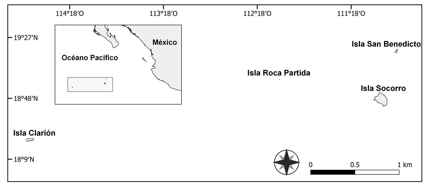
Figura 1. Localización del Parque Nacional Revillagigedo. El límite del área natural protegida está indicado con el recuadro punteado. Mapa por Miriam Hueytletl-Pérez.
Para medir el grado en el cual las especies están relacionadas taxonómicamente unas con otras y el grado por el cual los taxones están alta o pobremente representados entre las islas, se estimó la distinción taxonómica promedio (Δ+) y su variación (Λ+) (Clarke y Warwick, 1999). Se usaron 5 categorías taxonómicas jerárquicas: especie, género, familia, orden y clase, las cuales se tomaron con base en la clasificación para equinodermos propuesta en WoRMS (2024). Los niveles taxonómicos fueron ponderados de la siguiente manera: w1, especies dentro del mismo género; w2, especies dentro de la misma familia, pero en diferente género; w3, especies dentro del mismo orden, pero en diferente familia, y así sucesivamente (Warwick y Clarke, 1995). Los embudos de la Δ+ y Λ+ se crearon con un intervalo de confianza de 95%. Todos los análisis estadísticos se realizaron con el programa PRIMER v6 (Clarke y Gorley, 2006).
Las abreviaturas utilizadas fueron, para asteroideos, R: radio mayor (medida del disco al brazo), r: radio menor (medida del disco al interadio), R/r: radio mayor entre el radio menor, AD: alto del disco. Para ofiuroideos, DD: diámetro del disco, LB: largo del brazo, AB: ancho del brazo (tomando la medida siempre en la vértebra 15).
Descripciones
Nuevos registros
Phylum Echinodermata Klein, 1778
Subphylum Asterozoa Zittel, 1895
Clase Asteroidea de Blainville, 1830
Orden Forcipulatida Perrier, 1884
Familia Asteriidae Gray, 1840
Género Astrometis Fisher, 1923
Astrometis sertulifera (Xantus, 1860)
Fig. 2
Material examinado: 1 individuo. Bahía Eclipse, isla Roca Partida, islas Revillagigedo, México, 19°00’32” N, 112°04’55.9” O: 1 ind. (ICML-UNAM 2.125.5), preservado en seco.
Descripción: R = 20.11 mm; r = 15.4 mm; R/r = 1.30 mm; AD = 16.98 mm. Disco pequeño, bien definido, sobresaliente, delimitado por placas abactinales que soportan cada espina medianamente larga, cónica y lisa. Cuerpo de aspecto espinoso (fig. 2A). El surco ambulacral es amplio, los pies ambulacrales presentan ventosa terminal (fig. 2B). Por cada mandíbula se encuentran 4 espinas orales y 2 suborales (fig. 2C). Del disco salen 5 radios estrechos en su base, angulares, moderadamente cónicos y con punta roma, ornamentados con espinas (fig. 2D). Madreporita redonda, con estrías irregulares. Las espinas abactinales son grandes, con la base más ancha que la punta, de aspecto cónico con punta roma. Las espinas marginales son de menor longitud que todas las demás de la superficie abactinal. Entre las placas abactinales se encuentran las áreas papulares en forma grupal e individualmente entre las espinas ambulacrales y adambulacrales de la superficie actinal. Las espinas adambulacrales se distinguen claramente, son largas, lisas, planas, presentes en 1 sola fila y con punta roma. Las espinas ambulacrales son similares, pero de menor tamaño. Cada espina abactinal y superomarginal se encuentra rodeada en su base o en algún punto longitudinal por un collar de pedicelarios no pedunculados cruzados, de tamaño mediano, bivalbados, dentados en la punta con la base empalmada (fig. 2E, F). Los pedicelarios se encuentran también dispersos en la superficie abactinal, diferenciados por los de alrededor de las espinas principalmente por un mayor tamaño.
Familia Heliasteridae Viguier, 1879
Género Heliaster Gray, 1840
Heliaster kubiniji Xantus, 1860
Fig. 3
Material examinado: 11 individuos. Bahía Eclipse, isla Roca Partida, islas Revillagigedo, México, 19°00’32” N, 112°04’55.9” O: 7 ind. (ICML-UNAM 2.62.2); 4 ind. (ICML-UNAM 2.62.3), preservado en seco.
Descripción: R = 22.24-68.37 mm; r = 12.33-37.43 mm; R/r (x̄) = 1.83 mm; AD = 4.69-25.98 mm. Disco grande con relación a los brazos, no elevado pero abultado en el centro, ornamentado con espinas abactinales cilíndricas robustas y de punta roma, unido a varios radios (de 21 a 24) deprimidos actinalmente, con espinas gruesas, cortas y con espineletas en el extremo distal, dispuestas en 4-6 hileras (fig. 3A, B). Una madreporita pequeña y estriada irregular y onduladamente (fig. 3C). Espinas que ornamentan la placa carinal son las más cilíndricas y gruesas de todas las espinas actinales. Placas marginales soportan espinas de aspecto cilíndrico con la punta aplanada. Superficie actinal plana, con espinas aplanadas en el extremo distal. Espinas ambulacrales en 1 hilera, surco ambulacral más amplio en la base del brazo que en la punta, podios con ventosa terminal (fig. 3D). Cuatro espinas orales por mandíbula, centrales aplanadas, largas, cónicas, con punta aguda, laterales del mismo aspecto, pero de menor longitud (fig. 3E). Pedicelarios en la superficie abactinal; cruzados y rectos, bivalbados, dispersos en todo el disco y más concentrados conforme se acerca la parte distal del radio, algunos cuantos dispersos también entre las espinas orales (fig. 3F).
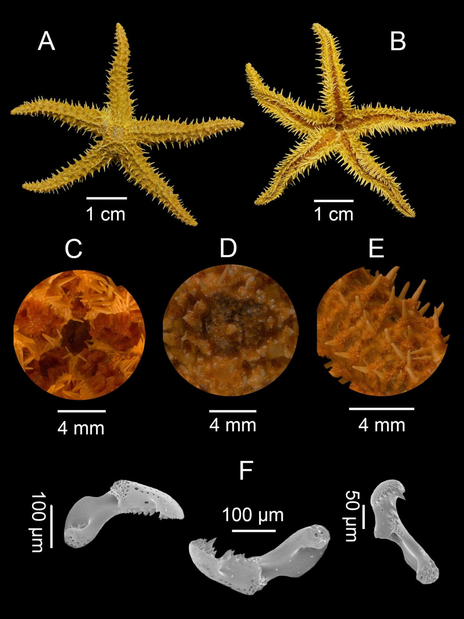
Figura 2. Astrometis sertulifera (ICML-UNAM 2.125.5). A, Ejemplar completo; vista abactinal; B. ejemplar completo; vista actinal; C, detalle de la mandíbula; espinas orales; D, detalle del disco; espinas que rodean el ano; E, detalle del brazo; espinas con montículos de pedicelarios en la base; F, valvas de pedicelarios rectos.
Clase Ophiuroidea Gray, 1840
Orden Amphilepidida O´Hara, Hugall, Thuy, Stöhr et Martynov, 2017
Familia Ophiolepididae Ljungman, 1867
Género Ophiolepis Müller et Troschel, 1840
Ophiolepis variegata Lütken, 1856
Fig. 4
Material examinado: 2 individuos. Bahía Eclipse, isla Roca Partida, islas Revillagigedo, México, 19°00’32” N, 112°04’559” O: 2 ind. (ICML-UNAM 3.26.3), preservado en seco.
Descripción: DD = 5.36-6.94 mm; LB = 12.00-20.00 mm; AB = 1.21-1.48 mm. Disco pentagonal. Disco dorsal (fig. 4A) cubierto por placas grandes rodeadas por placas más pequeñas, todas con arreglo muy definido; placa central del disco casi redonda, rodeada por 5 placas pentagonales más o menos regulares que forman una roseta; de este sistema de placas centrales irradian 5 hileras que abarcan hasta los márgenes interradiales. Gran placa cuadrangular entre la base de los radios y la parte distal de los escudos radiales. Escudos radiales grandes, en forma de gota. Interradio cubierto por placas grandes de forma y tamaño irregular (fig. 4B). Escudos orales pentagonales con el borde distal alargado, más largos que anchos, angostos en su parte media (fig. 4C). Escudos adorales pequeños, en contacto entre sí (fig. 4C). Cuatro papilas orales triangulares a cada lado de la mandíbula (fig. 4C). Cinco brazos robustos. Placas dorsales trapezoidales con bordes rectos, más anchas que largas (fig. 4D). Placas accesorias pequeñas, segmentadas en 2 piezas. Placas ventrales heptagonales, más anchas que largas (fig. 4E). Dos escamas tentaculares grandes, predominando en tamaño la adradial. De 3 a 4 espinas de los brazos, cortas y puntiagudas. Coloración del disco beige con algunas manchas gris oscuro dispersas; brazos en vista dorsal con bandas beige y gris oscuro, abarcando 1-3 segmentos (fig. 4A).
Famlia Ophiopsilidae Matsumoto, 1915
Género Ophiopsila Forbes, 1843
Ophiopsila californica A. H. Clark, 1921
Fig. 5
Material examinado: 1 individuo. Isla Roca Partida, islas Revillagigedo, México, 19°00’32” N, 112°04’55” O: 1 ind. (ICML-UNAM 3.102.2), preservado en alcohol al 70%.
Descripción: DD = 6.08 mm; LB = 48.48 mm; AB = 1.48 mm. Disco cubierto dorsal y ventralmente por numerosas escamas pequeñas, redondeadas e imbricadas, con apariencia de piel (fig. 5A, B). Escudos radiales largos y delgados, con aspecto triangular. Escudos orales casi tan largos como anchos, triangulares, ángulos laterales redondeados, ligeramente cóncavos. Escudos adorales pequeños, difíciles de distinguir (fig. 5C). Dos papilas orales puntiagudas a cada lado de la mandíbula, la más distal de mayor tamaño (fig. 5C). Cinco brazos delgados. Placas dorsales de los brazos casi tan largas como anchas, ovaladas, en contacto unas con otras (fig. 5D). Placas ventrales de los brazos más largas que anchas, cuadrangulares (fig. 5E). Dos escamas tentaculares, la adradial con forma de hoja, muy larga, llegándose a cruzar distalmente con la adradial contigua, la abradial de menor tamaño. Cinco espinas de los brazos no tan largas, con punta roma, la de en medio la más larga y robusta. Coloración del disco amarillenta con puntos negros tanto dorsal como ventralmente (fig. 5B). Brazos dorsalmente amarillos con bandas transversales marrón (usualmente compuesto por 3 placas), placas claras; brazo con una línea clara que lo recorre longitudinalmente desde la base hasta la punta (fig. 5B). Algunas placas dorsales y espinas de los brazos presentan puntos.
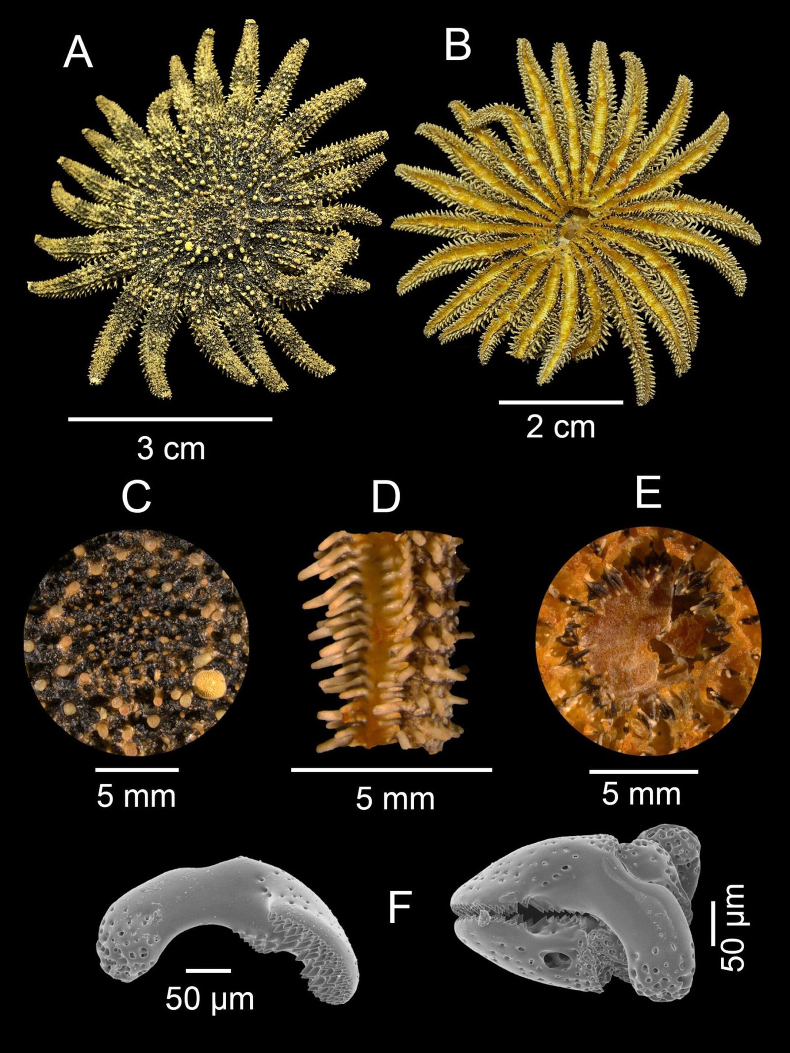
Figura 3. Heliaster kubiniji (ICML-UNAM 2.62.2). A, Ejemplar completo; vista abactinal; B, ejemplar completo; vista actinal; C, detalle del disco; espinas que rodean el ano y madreporita; D, detalle del brazo; canal ambulacral, espinas ambulacrales y adambulacrales; espinas superomarginales e infoeromarginales; E, detalle de la mandíbula; espinas orales; F, valva aislada de un pedicelario recto y un pedicelario recto ensamblado.
Familia Ophiotrichidae Ljungman, 1867
Género Ophiothela Verrill, 1867
Ophiothela mirabilis (Verrill, 1867)
Fig. 6
Material examinado: 4 individuos. Caleta Norte, isla Clarión, islas Revillagigedo, México, 19°22’14.3” N, 114°41’40.7” O: 1 ind. (LEMA-EQ 829), 23/abril/2023, 20 m, preservado en alcohol al 96%; 3 ind. (LEMA-EQ 831), Punta Tosca, isla Socorro, islas Revillagigedo, México, 18°46’47.8” N, 111°02’49.7” O, 25/abril/2023, 20 m, preservado en alcohol al 96%.
Descripción: DD = 1.45 mm; LB = 4.54-6.04 mm; AB = 0.20-0.24 mm. Disco rosetado, dorsalmente cubierto con piel y gránulos (fig. 6A). Escudos radiales en contacto, cubriendo casi todo el disco, parcialmente cubiertos por gránulos. Interradio cubierto con piel (fig. 6B). Escudos orales y adorales unidos formando un anillo continuo alrededor de la boca, cubiertos totalmente por piel (fig. 6C). Sin papilas orales (fig. 6C). Cerca de 10 papilas dentales. Seis brazos prensiles. Placas dorsales de los brazos cubiertas por pocos gránulos de tamaño irregular, espacio de piel entre las placas (fig. 6D). Placas ventrales de los brazos cubiertas por piel (fig. 6E). De 5 a 6 espinas de los brazos, aserradas en la punta y en forma de gancho, la más dorsal es la de menor tamaño. Sin escamas tentaculares. Coloración dorsal del disco y brazos morado-rosáceo (fig. 6A).
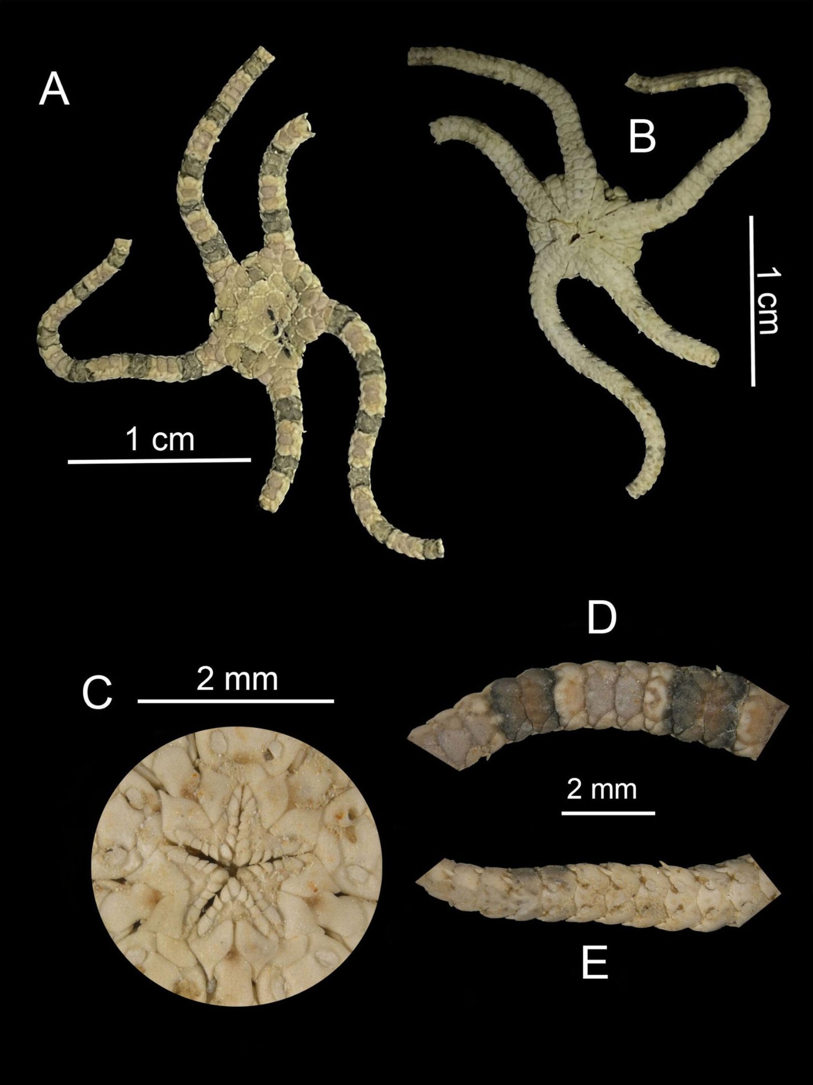
Figura 4. Ophiolepis variegata (ICML-UNAM 3.26.3). A, Ejemplar completo, vista dorsal; B, ejemplar completo, vista ventral; C, detalle de la mandíbula; D, detalle del brazo, vista dorsal; E, detalle del brazo, vista ventral.
Riqueza de especies
Como resultado de la revisión histórica y los nuevos registros previamente mencionados, en total se registraron 94 especies de equinodermos (tabla 1), de las cuales 21 corresponden a la clase Asteroidea, 31 a Ophiuroidea, 21 a Echinoidea y 21 a Holothuroidea (tabla 2). La mayor riqueza de equinodermos se encontró en las islas Clarión (60 spp.) y Socorro (58 spp.), mientras que la menor en Roca Partida (20 spp.) y San Benedicto (10 spp.). El mayor número de especies de crinoideos, asteroideos, ofiuroideos y equinoideos se tuvo en la isla Clarión, y para holoturoideos se presentó en la isla Socorro (tabla 2).
El 4% de las especies (Asteroidea: Acanthaster planci, Mithrodia bradleyi; Echinoidea: Echinometra vanbrunti y Eucidaris thouarsii) han sido registradas en todas las islas. En contraste, el 51% (49 spp.) habitan en solo 1 de las 4 islas. El 7% (7 spp.) (Asteroidea: Mediaster transfuga;Ophiuroidea: Ophiacantha moniliformis, Ophiopholis bakeri, Ophiothrix (Ophiothrix) rudis y Ophiothrix (Ophiothrix) spiculata;Holothuroidea: Euthyonidiella zacae y Holothuria (Mertensiothuria) hilla)han sido reportadas para el archipiélago, pero no se especifica en qué isla fueron encontradas (Granja-Fernández et al., 2015, 2021; Honey-Escandón et al., 2008; Solís-Marín et al., 2013).
Tabla 1
Lista de especies de equinodermos del Parque Nacional Revillagigedo. IS = Isla Socorro, IC = isla Clarión, IB = isla San Benedicto, IR = isla Roca Partida, NE = isla no especificada. *Nuevos registros para cada isla. Especies en negritas corresponden a registros nuevos para el Parque Nacional Revillagigedo.
| Clase | Especie |
| Asteroidea | Acanthaster planci (Linnaeus, 1758) IS, IC, IB, IR* |
| Asteropsis carinifera (Lamarck, 1816) IS, IC | |
| Astrometis sertulifera(Xantus, 1860) IR* | |
| Astropecten armatus Gray, 1840 IC | |
| Heliaster kubinijiXantus, 1860 IR* | |
| Henricia clarki Fisher, 1910 IC | |
| Henricia seminudus (A.H. Clark, 1916) IC | |
| Linckia columbiae Gray, 1840 IS, IC | |
| Luidia bellonae Lütken, 1864 IC | |
| Luidia columbia (Gray, 1840) IC | |
| Mediaster transfuga Ludwig, 1905 NE | |
| Meridiastra modesta (Verrill, 1867) IS | |
| Mithrodia bradleyi Verrill, 1867 IS, IC, IB, IR* | |
| Nearchaster (Nearchaster) aciculosus (Fisher, 1910) IC | |
| Nidorellia armata (Gray, 1840) IB | |
| Patiria miniata (Brandt, 1835) IS | |
| Pauliastra aenigma (Ludwig, 1905) IC | |
| Pentaceraster cumingi (Gray, 1840) IS, IC, IR* | |
| Tabla 1. Continúa | |
| Clase | Especie |
| Pharia pyramidata (Gray, 1840) IS | |
| Phataria unifascialis (Gray, 1840) IS | |
| Sclerasterias heteropaes Fisher, 1924 IC | |
| Ophiuroidea | Amphipholis pugetana (Lyman, 1860) IC |
| Amphiura seminuda Lütken et Mortensen, 1899 IC | |
| Astrodictyum panamense (Verrill, 1867) IR | |
| Ophiacantha diplasia H.L. Clark, 1911 IC | |
| Ophiacantha moniliformis Lütken et Mortensen, 1899 NE | |
| Ophiacantha pyriformis Ziesenhenne, 1937 IC | |
| Ophiactis savignyi (Müller et Troschel, 1842) IS*, IC, IR* | |
| Ophiactis simplex (Le Conte, 1851) IS* | |
| Ophiocoma aethiops Lütken, 1859 IS, IC | |
| Ophiocomella alexandri (Lyman, 1860) IS, IC, IR* | |
| Ophiocomella schmitti A.H. Clark, 1939 IS, IC | |
| Ophiocomella sexradia (Duncan, 1887) IC | |
| Ophioderma aija Humara-Gil, Granja-Fernández, Bautista-Guerrero, Solís-Marín et Rodríguez-Troncoso, 2024 IS Ophioderma bichi Humara-Gil, Granja-Fernández, Bautista-Guerrero, Solís-Marín et Rodríguez-Troncoso, 2024 IR Ophioderma hendleri Granja-Fernández, Pineda-Enríquez, Solís-Marín et Laguarda-Figueras, 2020 IS | |
| Ophioderma occultum Humara-Gil, Granja-Fernández, Bautista-Guerrero et Rodríguez-Troncoso, 2022 IS*, IR | |
| Ophioderma panamense Lütken, 1859 IS, IC | |
| Ophioderma variegatum Lütken, 1856 IS, IC | |
| Ophiolepis pacifica Lütken, 1856 IS | |
| Ophiolepis variegataLütken, 1856 IR* | |
| Ophiomyxa panamensis Lütken et Mortensen, 1899 IS | |
| Ophionereis annulata (Le Conte, 1851) IS, IC, IR* | |
| Ophiopholis bakeri McClendon, 1909 NE | |
| Ophiophragmus papillatus Ziesenhenne, 1940 IS | |
| Ophiopsila californicaA.H. Clark, 1921 IR* | |
| Ophiosphalma variabile (Lütken et Mortensen, 1899) IC | |
| Ophiothela mirabilis(Verrill, 1867) IS*, IC* | |
| Ophiothrix galapagensis Lütken et Mortensen, 1899 IC | |
| Ophiothrix (Ophiothrix) rudis Lyman, 1874 NE | |
| Ophiothrix (Ophiothrix) spiculata Le Conte, 1851 NE | |
| Ophiuroconis bispinosa Ziesenhenne, 1937 IS | |
| Echinoidea | Astropyga pulvinata (Lamarck, 1816) IS |
| Brissopsis pacifica (A. Agassiz, 1898) IS, IC | |
| Clypeaster europacificus H.L. Clark, 1914 IC | |
| Tabla 1. Continúa | |
| Clase | Especie |
| Clypeaster ochrus H.L. Clark, 1914 IC | |
| Clypeaster rotundus (A. Agassiz, 1863) IC | |
| Clypeaster speciosus Verrill, 1870 IS, IC | |
| Diadema mexicanum A. Agassiz, 1863 IS, IC, IB | |
| Echinometra insularis H. L. Clark, 1912 IS | |
| Echinometra oblonga (Blainville, 1825) IS, IC | |
| Echinometra vanbrunti A. Agassiz, 1863 IS, IC, IB, IR* | |
| Encope micropora insularis H.L. Clark, 1948 IS, IC | |
| Eucidaris thouarsii (L. Agassiz et Desor, 1846) IS, IC, IB, IR* | |
| Heterocentrotus mamillatus (Linnaeus, 1758) IS, IC, IB | |
| Hesperocidaris asteriscus H.L. Clark, 1948 IS | |
| Hesperocidaris perplexa (H.L. Clark, 1907) IC | |
| Lovenia cordiformis A. Agassiz, 1872 IS, IC | |
| Meoma ventricosa grandis Gray, 1851 IS, IC | |
| Rhyncholampas pacificus (A. Agassiz, 1863) IS, IC | |
| Toxopneustes roseus (A. Agassiz, 1863) IS, IC | |
| Tripneustes depressus A. Agassiz, 1863 IS, IC, IB | |
| Tripneustes gratilla (Linnaeus, 1758) IC | |
| Holothuroidea | Euapta godeffroyi (Semper, 1868) IS, IR* |
| Euthyonidiella zacae (Deichmann, 1938) NE | |
| Holothuria (Cystipus) inhabilis Selenka, 1867 IC | |
| Holothuria (Halodeima) inornata Semper, 1868 IS, IC | |
| Holothuria (Halodeima) kefersteinii (Selenka, 1867) IS, IC | |
| Holothuria (Lessenothuria) coronata Yánez Villanueva, Solís-Marín et Laguarda-Figueras, 2022 IS | |
| Holothuria (Mertensiothuria) hilla Lesson, 1830 NE | |
| Holothuria (Mertensiothuria) leucospilota (Brandt, 1835) IS, IC | |
| Holothuria (Platyperona) difficilis Semper, 1868 IS, IC | |
| Holothuria (Selenkothuria) lubrica Selenka, 1867 IS, IC, IR* | |
| Holothuria (Selenkothuria) portovallartensis Caso, 1954 IS, IC | |
| Holothuria (Semperothuria) imitans Ludwig, 1875 IS, IC, IR* | |
| Holothuria (Stauropora) fuscocinerea Jaeger, 1833 IS*, IC, IB* | |
| Holothuria (Theelothuria) paraprinceps Deichmann, 1937 IC | |
| Holothuria (Thymiosycia) arenicola Semper, 1868 IS, IC | |
| Holothuria (Thymiosycia) impatiens (Forsskål, 1775) IS, IR* | |
| Isostichopus fuscus (Ludwig, 1875) IS, IB*, IR* | |
| Labidodemas americanum Deichmann, 1938 IS* | |
| Leptosynapta albicans (Selenka, 1867) IS | |
| Lisacucumis gibber (Selenka, 1867) IS | |
| Pentamera chierchiae (Ludwig, 1886) IS |
Tabla 2
Riqueza de especies para cada clase de equinodermos del Parque Nacional Revillagigedo y para cada una de sus islas. * Registros que no tienen una isla especificada.
| Clase | Total | Isla Socorro | Isla Clarión | Isla San Benedicto | Isla Roca Partida | *No especificado |
| Asteroidea | 21 | 9 | 13 | 3 | 5 | 1 |
| Ophiuroidea | 31 | 16 | 18 | 0 | 8 | 4 |
| Echinoidea | 21 | 16 | 18 | 5 | 2 | 0 |
| Holothuroidea | 21 | 17 | 11 | 2 | 5 | 3 |
| Total | 94 | 58 | 60 | 10 | 20 | 8 |
Similitud entre islas
La comparación de riqueza con los análisis de clasificación y nMDS entre las islas del PNR mostró 2 grupos bien definidos, un primer grupo formado por las islas Socorro y Clarión con 40% de similitud (Simprof, π = 0, p > 0.05) y el segundo formado por San Benedicto y Roca Partida con 20% de similitud (Simprof, π = 0, p > 0.05) (fig. 7A).
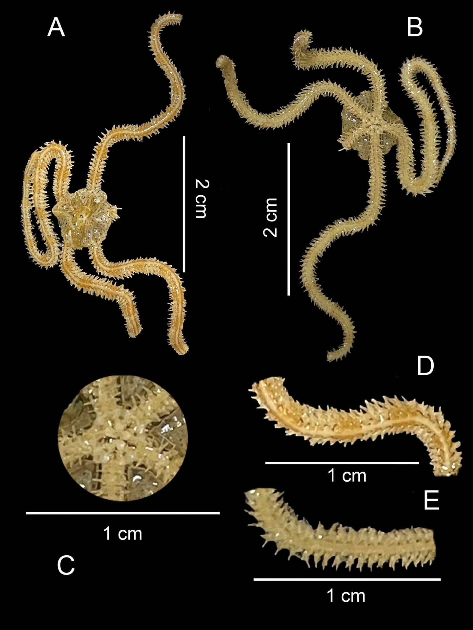
Figura 5. Ophiopsila californica (ICML-UNAM 3.102.2). A, Ejemplar completo, vista dorsal; B, ejemplar completo, vista ventral; C, detalle de la mandíbula; D, detalle del brazo, vista dorsal; E, detalle del brazo, vista ventral.
Diversidad taxonómica de las islas
El modelo global de Δ+ y Λ+ entre las islas del archipiélago mostró que todas las islas poseen una diversidad taxonómica y variación dentro del intervalo de confianza del 95% esperado (p > 0.05) (fig. 7B). Roca Partida tuvo la mayor Δ+, a pesar de que Socorro y Clarión son las islas con una mayor riqueza de especies. San Benedicto presentó la menor Δ+. Las estimaciones de Λ+ para cada una de las islas estuvieron dentro de las estimaciones de probabilidad (fig. 7C).
Discusión
La revisión taxonómica de los especímenes depositados en colecciones científicas del presente trabajo permitió encontrar 2 nuevos registros de asteroideos (Astrometis sertulifera y Heliaster kubiniji) y 3 de ofiuroideos (Ophiolepis variegata, Ophiopsila californica y Ophiothela mirabilis) para el PNR. Con lo anterior se actualiza el inventario a 94 especies y con los nuevos registros se incrementa la riqueza de especies a 21 para la clase Asteroidea y 31 para Ophiuroidea. Anteriormente, el ofiuroideo Ophioderma teres se reportó para el PNR (Granja-Fernández et al., 2021); sin embargo, la reciente revisión taxonómica de la especie permitió determinar que su identidad corresponde a Ophioderma aija (Humara-Gil et al., 2024), por lo tanto, el registro de O. teres para el PNR se invalida. Al igual que lo reportado por Granja-Fernández et al. (2021), no se encontraron registros verificados de ejemplares de la clase Crinoidea para Revillagigedo. El único registro que se tenía de un crinoideo es el descrito por Roux y Pawson (1999), que corresponde a la especie Hyocrinus foelli, una especie encontrada entre Clarión y la zona de fractura de Clipperton a una profundidad de entre 4,300 y 4,700 m; sin embargo, este no se considera válido, ya que al verificar las coordenadas geográficas del ejemplar recolectado, se encontró distante del límite del parque (Granja-Fernández et al., 2021). La diferencia en riqueza de especies entre trabajos se debe a la actualización del inventario mediante la consulta de literatura, nuevas descripciones y la revisión taxonómica de material depositado en colecciones científicas.
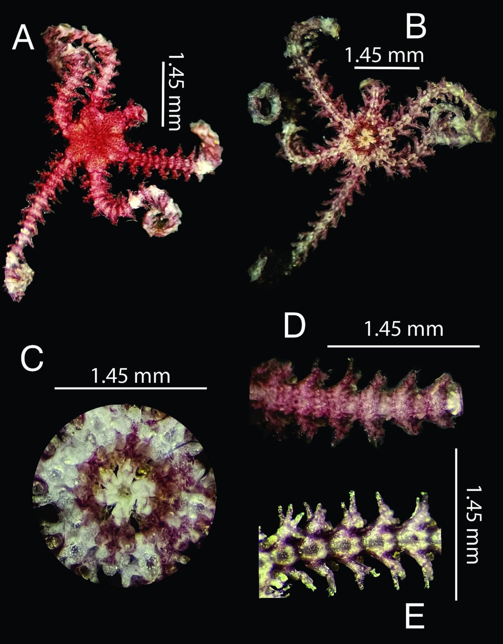
Figura 6. Ophiothela mirabilis (LEMA-EQ 831). A, Ejemplar completo, vista dorsal; B, ejemplar completo, vista ventral; C, detalle de la mandíbula; D, detalle del brazo, vista dorsal; E, detalle del brazo, vista ventral.
El registro del asteroideo Astrometis sertulifera para Roca Partida corresponde a un nuevo registro para el PNR, así como para el Pacífico central mexicano, ya que la especie solo había sido reportada en México para la costa oeste de Baja California y el golfo de California (Honey-Escandón et al., 2008; Solís-Marín et al., 2005). Por otro lado, Heliaster kubiniji fue reportada por Bautista-Romero et al. (1994) para isla Clarión, sin embargo, al no poder ser confirmado por la falta de un ejemplar que permitiera la validación, no fue incluida en el recuento de Granja-Fernández et al. (2021). La revisión de material depositado en la colección del ICML-UNAM permitió corroborar su presencia en el PNR, específicamente en isla Roca Partida. La distribución de esta estrella es muy amplia, abarcando México, las islas Galápagos y Perú (Solís-Marín et al., 2013). La especie es más común en el golfo de California en México, sin embargo, se ha reportado que se presentan registros ocasionales dispersos hacia el noroeste de Baja California y el sur de California (EUA), los cuales probablemente están asociados a eventos de El Niño (Kerstitch y Bertsch, 2007).
Tres nuevos registros de ofiuros se lograron identificar con base en ejemplares de las colecciones ICML-UNAM y LEMITAX. Ophiolepis variegata ha sido previamente registrada a lo largo de la costa del Pacífico mexicano (Granja-Fernández et al., 2015) y específicamente en el Pacífico central mexicano, en Nayarit, Jalisco, Colima e islas Marías (Granja-Fernández et al., 2021); sin embargo, su hallazgo en el PNR (isla Roca Partida) corresponde a un registro nuevo para el archipiélago. El caso de Ophiopsila californica es de particular importancia ya que su distribución comprende desde California hasta el norte del Pacífico mexicano (Granja-Fernández et al., 2015). Su recolecta en isla Roca Partida no solo corresponde a un registro nuevo para el Pacífico central mexicano, sino también a una ampliación de su rango de distribución al sur. Finalmente, a pesar de que Ophiothela mirabilis se encuentra ampliamente distribuida en el Pacífico mexicano (Granja-Fernández et al., 2015), esta es la primera vez que se registra en el PNR, específicamente para las islas Clarión y Socorro.
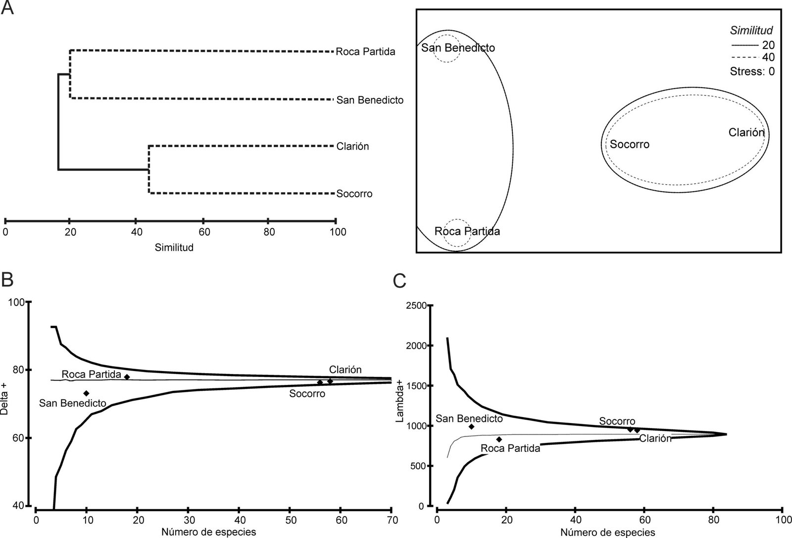
Figura 7. A, Análisis de clasificación y NMDS para analizar la similitud de especies entre las islas del archipiélago de Revillagigedo. Las líneas segmentadas en el dendrograma indican los grupos identificados por la prueba Simprof; B, estimaciones de la distinción taxonómica promedio (Δ+) y C, de su variación (Λ+) para los grupos de equinodermos de las islas de Revillagigedo. Los intervalos de confianza al 95% se muestran en líneas continuas y Δ+ y Λ+ se muestran en una línea segmentada.
Cabe destacar que el presente trabajo analiza por primera vez la riqueza de equinodermos para cada una de las islas del PNR. Las islas Clarión (61) y Socorro (58), además de poseer la mayor riqueza de equinodermos total y por clases, se agruparon dentro de los análisis nMDS y dendrograma, compartiendo 35 especies. San Benedicto y Roca Partida formaron otro grupo, con una baja similitud, donde comparten solamente 5 especies. Los valores de riqueza de especies pueden estar relacionados con el tamaño de las islas. En este caso, las islas más grandes (Socorro y Clarión) presentan el mayor número de especies y, por el contrario, las islas más pequeñas (San Benedicto y Roca Partida) tienen la menor riqueza de especies. Este patrón puede no estar asociado solamente con el tamaño de las islas, sino también con los hábitats que proporcionan y con la intensidad de muestreo en cada una de ellas. Clarión y Socorro se caracterizan por playas de material calcáreo biogénico asociado con corales, así como con sedimentos (arenas y limos) conformados por moluscos y corales, crecimientos algales, entre otros (Semarnat-Conanp, 2019). Todos estos hábitats son propicios para el establecimiento de larvas (Doll et al., 2022), protección/desarrollo (Hermosillo-Núñez et al., 2015; Herrero-Pérezrul et al., 2015) y alimentación de equinodermos (Siburian et al., 2023). Esta heterogeneidad en la estructura de los hábitats no se presenta en San Benedicto y Roca Partida, ya que la primera está compuesta, principalmente, de rocas volcánicas y la segunda es la cima de un volcán submarino (Semarnat-Conanp, 2019).
Respecto de la intensidad de muestreo, la exploración de Clarión y Socorro ha llamado la atención de científicos desde 1930 y han sido visitadas desde entonces por expediciones tan importantes como Albatross, Velero y Zaca (Caso, 1962; Deichmann, 1941; Ziesenhenne, 1937). Resultado de lo anterior es que Clarión y Socorro poseen el mayor número de estudios publicados (41 y 47 trabajos, respectivamente) con registros de equinodermos de zonas someras y profundas. En cambio, para San Benedicto solo existen 2 trabajos (Bautista-Romero et al., 1994; Reyes-Bonilla, 1995) en los que se reportan 8 especies de las clases Asteroidea y Echinoidea; con la presente revisión de colecciones científicas, se añaden 2 nuevos registros de holoturoideos para San Benedicto (Holothuria (Stauropora) fuscocinerea e Isostichopus fuscus). Previo a este estudio, el único equinodermo que había sido reportado para la isla Roca Partida era el ofiuro Astrodictyum panamense (Ayala-Bocos et al., 2011), por lo que se aportan 17 nuevos registros para esta isla (5 de la clase Asteroidea, 5 de Ophiuroidea, 2 de Echinoidea y 5 Holothuroidea). A pesar de que San Benedicto y Roca Partida tienen la menor riqueza de equinodermos, no se descarta que con mayor esfuerzo de muestreo se encuentre una mayor riqueza de equinodermos en estas islas.
A pesar de las diferencias en riqueza entre islas, existen 4 especies que han sido registradas en todas ellas: 2 asteroideos (Acanthaster planci y Mithrodia bradleyi)y 2 equinoideos (Echinometra vanbrunti y Eucidaris thouarsii). Sin embargo, especies como la estrella de mar Pentaceraster cumingi, el ofiuro Ophiocomella alexandri, el erizo Toxopneustes roseus y el pepino I. fuscus, se espera que habiten en todas las islas y sus alrededores, ya que tienen una amplia distribución a lo largo del Pacífico mexicano y americano (Granja-Fernández et al., 2015, 2021; Honey-Escandón et al., 2008; Solís-Marín et al., 2013). También cabe resaltar que, a pesar de las diferencias en riqueza, el análisis de diversidad taxonómica sugiere que la composición de cada isla es un subconjunto al azar del conjunto regional de especies, ya que los valores se encontraron dentro del intervalo de confianza de 95%, es decir, todas las islas son representativas de la diversidad taxonómica del PNR, inclusive San Benedicto y Roca Partida, que tienen la menor riqueza de especies.
La riqueza de especies de equinodermos del PNR representa cerca de 15% de la riqueza registrada en todo México (Solís-Marín et al., 2013, 2014). Si se compara la riqueza de manera particular con las diferentes regiones del Pacífico mexicano como el golfo de California y el Pacífico mexicano, encontramos que el PNR presenta 40.5% y 43.5% de especies, respectivamente. Comparando con la región del Pacífico central mexicano, en el parque se encuentra 50% de estas especies (Granja-Fernández et al., 2021). Esto respalda la importancia de Revillagigedo en términos de conservación, ya que resguarda cerca de la mitad de especies de equinodermos que se pueden encontrar en el Pacífico mexicano.
Para generar un inventario más completo de las especies de equinodermos presentes en el PNR se requiere una búsqueda dirigida al grupo y a los distintos sustratos en los que habitan (e.g., arena, rocas, corales). Se recomienda incrementar el esfuerzo de muestreo principalmente en San Benedicto y Roca Partida. Asimismo, si bien la mayor parte de registros pertenecen a especies someras (< 30 m de profundidad), es necesaria la exploración de aguas profundas del PNR y sus alrededores, ya que poseen un alto potencial de albergar equinodermos por su amplia batimetría que puede alcanzar hasta 5,000 m de profundidad y a la presencia de ventilas hidrotermales (Semarnat-Conanp, 2019). También es necesario dirigir esfuerzos sobre especies crípticas, las cuales regularmente están ocultas y cuya percepción no es tan sencilla en su hábitat (principalmente especies de las clases Ophiuroidea y Holothuroidea), ya que suelen encontrarse bajo rocas o enterradas en el sedimento.
Agradecimientos
Al personal de Conanp del Parque Nacional Revillagigedo por la invitación a CMGV y ODD para participar en la expedición científica 2023. Al personal del Instituto de Biología de la UNAM, Susana Guzmán Gómez y María B. Mendoza Garfias; al personal del ICML de la UNAM, Laura E. Gómez Lizárraga, Alicia Durán González y Carlos A. Conejeros Vargas, por su disposición y colaboración para la realización de este estudio. A Brenda Maya Alvarado por la consulta de referencias bibliográficas que nutren este artículo y a Karla Humara Gil por la corroboración de registros por isla para el género Ophioderma. Agradecemos el apoyo técnico para la captura de imágenes de Alicia Durán González, María B. Mendoza Garfias, Susana Guzmán Gómez y Laura E. Gómez Lizárraga de la UNAM. Al editor y revisores anónimos por sus comentarios invaluables al manuscrito.
Referencias
Ayala-Bocos, A., Reyes-Bonilla, H., Herrero-Perezrul M. D., Walther-Mendoza, M. y Castañeda-Fernández de Lara, V. (2011). New records and range extensions of Astrodictyum panamense (Ophiuroidea: Gorgonocephalidae) in the Eastern Pacific Ocean. Marine Biodiversity Records. Marine Biological Association of the United Kingdom, 4, e46. https://doi.org/10.1017/S175526721100032
Bautista-Romero, J. J., Reyes-Bonilla, H., Lluch-Cota, D. y Lluch-Cota, S. (1994). Aspectos generales de la fauna marina. En A. Ortega-Rubio y A. Castellanos-Vera (Eds.), La isla Socorro, Reserva de la Biosfera Archipiélago de Revillagigedo (pp. 247–275). La Paz: CIBNOR.
Becerril-García, E. E., Hoyos-Padilla, E. M., Henning, B. y León, P. S. (2020). Sharks, rays, and chimaeras of the Revillagigedo National Park: An update of new and confirmed records. Journal of Fish Biology, 97, 1228–1232. https://doi.org/10.1111/jfb.14457
Caso, M. E. (1962). Estudios sobre equinodermos de México. Contribución al conocimiento de los equinodermos de las islas Revillagigedo. Anales del Instituto de Biología, Universidad Nacional Autónoma de México, 33, 293–330.
Clark, A. H. (1921). A new ophiuran of the genus Ophiopsila from Southern California. Proceedings of the Biological Society of Washington, 34, 109–110.
Clark, H. L. (1907). The Cidaridae. Bulletin of the Museum of Comparative Zoology, 7, 165–230.
Clarke, K. R. y Gorley, R. N. (2006). Primer v6: user manual and tutorial. Plymouth, UK: Primer-E.
Clarke, K. R., Somerfield, P. J. y Gorley, R. N. (2008). Testing of null hypotheses in exploratory community analyses: similarity profiles and biota-environment linkage. Journal of Experimental Marine Biology and Ecology, 366, 56–69. https://doi.org/10.1016/j.jembe.2008.07.009
Clarke, K. R. y Warwick, R. M. (1999). The taxonomic distinctness measure of biodiversity: weighting of step lengths between hierarchical levels. Marine Ecology Progress Series, 184, 21–29.
Conabio (Comisión Nacional para el Conocimiento y Uso de la Biodiversidad)-Conanp (Comisión Nacional de Áreas Naturales Protegidas) -TNC-Pronatura. (2007). Sitios marinos prioritarios para la conservación de la biodiversidad. Escala 1: 1000 000. México: Comisión Nacional para el Conocimiento y Uso de la Biodiversidad, Comisión Nacional de Áreas Naturales Protegidas/ The Nature Conservancy – Programa México, Pronatura, A.C.
Conanp (Comisión Nacional de Áreas Naturales Protegidas)-Semarnat (Secretaría de Medio Ambiente y Recursos Naturales). (2015). Formulario de Nominación del Bien Natural Archipiélago de Revillagigedo para su Inscripción en la Lista del Patrimonio Mundial. México D.F.: Comisión Nacional de Áreas Naturales Protegidas, Secretaría de Medio Ambiente y Recursos Naturales.
Conanp (Comisión Nacional de Áreas Naturales Protegidas)-Semarnat (Secretaría de Medio Ambiente y Recursos Naturales). (2017). Estudio Previo Justificativo para la declaratoria del Parque Nacional Revillagigedo. México: Comisión Nacional de Áreas Naturales Protegidas, Secretaría de Medio Ambiente y Recursos Naturales.
Deichmann, E. (1937). The Templeton Crocker Expedition. IX. Holothurians from the Gulf of California, the West Coast of Lower California and Clarion Island. Zoologica, 22, 161–176.
Deichmann, E. (1941). The Holothuroidea collected by the “Velero III” during the years 1932-1938. Part I. Dendrochirotida. Allan Hancock Pacific Expeditions, 8, 61–195.
Diario Oficial de la Federación (DOF). (2017). Decreto por el que se declara como Área Natural Protegida, con el carácter de Parque Nacional, la región conocida como Revillagigedo, localizada en el Pacífico Mexicano. Publicada en el Diario Oficial de la Federación el 27 de noviembre de 2017. México. Recuperado el 21 de enero, 2024 de: https://www.gob.mx/epn/prensa/comunicado-136165
Doll, P. C., Caballes, C. F., Hoey, A. S., Uthicke, S., Ling, S. D. y Pratchett, M. S. (2022). Larval settlement in echinoderms: a review of processes and patterns. Oceanography and Marine Biology: An Annual Review, 60, 433–494. https://doi.org/10.1201/9781003288602-9
Fisher, W. K. (1911). Asteroidea of the North Pacific and adjacent waters, Part I: Phanerozonia and Spinulosa. Bulletin of the United States National Museum, 76, 1–419.
Granja-Fernández, M. R., Herrero-Pérezrul, M. D., López-Pérez, R. A., Hernández-Morales, A. y Rangel-Solís, P. D. (2015). A literature review of the Ophiuroidea (Echinodermata) from the Pacific coast of Mexico. Revista de Biología Tropical, 63, 37–47. http://dx.doi.org/10.15517/rbt.v63i2.23127
Granja-Fernández, M. R., Maya-Alvarado, B., Cupul-Magaña, A. L., Rodríguez-Troncoso, A. P., Solís-Marín, F. A. y Sotelo-Casas, R. C. (2021). Echinoderms (Echinodermata) from the Central Mexican Pacific. Revista de Biología Tropical, 69, 219–259. http://dx.doi.org/10.15517/rbt.v69isuppl.1.46356
Hermosillo-Núñez, B. B., Rodríguez-Zaragoza, F. A., Ortiz, M., Galván-Villa, C., Cupul-Magaña A. y Ríos-Jara, E. (2015). Effect of habitat structure on the most frequent echinoderm species inhabiting coral reef communities at Isla Isabel National Park (Mexico). Community Ecology, 16, 125–134. https://doi.org/10.1556/168.2015.16.1.14
Herrero-Pérezrul, M. D., Ramírez-Ortíz, G., Rosales-Estrada, M. y Reyes-Bonilla, H. (2015). Densidad poblacional y distribución espacial de erizos de mar (Echinodermata: Echinoidea) en la isla Socorro, Archipiélago de Revillagigedo, México. Revista de Biología Tropical, 63, 221–232. https://doi.org/10.15517/rbt.v63i2.23156
Honey-Escandón, M., Solís-Marín, F. A. y Laguarda-Figueras, A. (2008). Equinodermos (Echinodermata) del Pacífico Mexicano. Revista de Biología Tropical, 56, 57–73. https://doi.org/10.15517/rbt.v56i3.27079
Humara-Gil, K. J., Granja-Fernández, R., Bautista-Guerrero, E., Solís-Marín, F. A. y Rodríguez-Troncoso, A. P. (2024). Delimitation of Ophioderma teres (Lyman, 1860) and Ophioderma unicolor H.L. Clark, 1940 stat. nov. (Echinodermata: Ophiuroidea), including the description of two new species. European Journal of Taxonomy, 947, 130–174. https://doi.org/10.5852/ejt.2024.947.2625
Kerstitch, A. y Bertsch, H. (2007). Sea of Cortez marine invertebrates. 2nd Edition. Monterey, CA: Sea Challengers.
Lütken, C. F. (1856). Bidrag til kundskab om Slangestjernerne. II. Oversigt over de vestindiske Ophiurer. Videnskabelige Meddelelser fra Dansk Naturhistorisk Förening i Kjøbenhavn 1856, 7, 1–26.
Pardo, M. y Suárez, G. (1995). Shape of the subducted Rivera and Cocos plates in southern Mexico: seismic and tectonic implications. Journal of Geophysical Research, 100, 357–373. https://doi.org/10.1029/95JB00919
Reyes-Bonilla, H. (1995). Asteroidea and Echinoidea (Echinodermata) of Isla San Benedicto, Revillagigedo Archipiélago, México. Revista de Investigación Científica UABCS, 6, 29–38.
Roux, M. y Pawson, D. L. (1999). Two new Pacific Ocean species of hyocrinid crinoids (Echinodermata), with comments on presumed giant-dwarf gradients related to seamounts and abyssal plains. Pacific Science, 53, 289–298.
Ruiz-Sakamoto, A., Sánchez-Ortiz, C., Stewart, J. D. y Aburto-Oropeza, O. (2018). La Manta Gigante el diamante de Revillagigedo. Biodiversitas, 136, 1–7.
Semarnat (Secretaría de Medio Ambiente y Recursos Naturales)-Conanp (Comisión Nacional de Áreas Naturales Protegidas). (2019). Programa de Manejo Parque Nacional Revillagigedo. México: Semarnat, Conanp.
Siburian, R. H. S., Tapilatu, J. R. y Tapilatu, M. E. (2023). Discovery of habitat preferences and community structure of echinoderms in Kri, Raja Ampat, Indonesia. Biodiversitas, 24, 3968–3976. https://doi.org/10.13057/biodiv/d240735
Solís-Marín, F. A., Honey-Escandón, M. B. I., Herrero- Pérezrul, M. D., Benítez-Villalobos, F., Díaz-Martínez, J. P., Buitrón-Sánchez, B. E. et al. (2013). The echinoderms of Mexico: biodiversity, distribution and current state of knowledge. En J. J. Alvarado y F. A. Solís-Marín (Eds.), Echinoderm research and diversity in Latin America. Berlín: Springer-Verlag. https://doi.org/10.1007/978-3-642-20051-9_2
Solís-Marín, F. A., Laguarda-Figueras, A., Durán-González, A., Gust, C. y Torres, J. (2005). Equinodermos (Echinodermata) del Golfo de California, México. Revista de Biología Tropical, 53, 123–137. https://doi.org/10.15517/rbt.v53i3
Solís-Marín, F. A., Laguarda-Figueras, A. y Honey-Escandón, M. (2014). Biodiversidad de equinodermos (Echinodermata) en México. Revista Mexicana de Biodiversidad, 85 (Suplem.),S441–S449. https://doi.org/10.7550/rmb.31805
Spalding, M. D., Fox, H. E., Allen, G. R., Davidson, N., Ferdaña, Z. A., Finlayson, M. et al. (2007). Marine ecoregions of the world: a bioregionalization of coastal and shelf areas. BioScience, 57, 573–583. https://doi.org/10.1641/B570707
Verrill, A. E. (1867). Notes on Radiata in the museum of Yale College with descriptions of new genera and species. No. 2. Notes on the echinoderms of Panama and the west coast of America, with descriptions of a new genus. Transactions of the Connecticut Academy of Arts and Sciences, 1, 251–322.
Warwick, R. M. y Clarke, K. R. (1995). New biodiversity measures reveal a decrease in taxonomic distinctness with increasing stress. Marine Ecology Progress Series, 129, 301–305.
WoRMS. (2024). World Register of Marine Species. Recuperado el 01 abril, 2024 de: https://www.marinespecies.org
Xantus, J. (1860). Descriptions of three new species of starfishes from Cape St. Lucas. Proceedings of the Academy of Natural Sciences of Philadelphia, 12, 568.
Ziesenhenne, F. C. (1937). The Templeton Crocker Expedition. X. Echinoderms from the West Coast of Lower California, the Gulf of California and Clarion Island. Zoology, 22, 209–239. https://doi.org/10.5962/p.184686

Continental turtles of southeastern Mexico: an update on the identification, composition, distribution and conservation
Eduardo Reyes-Grajales a, b, *, Christian Rico c, John Iverson d, Luis Díaz-Gamboa e, Marco A. López-Luna f, Wilfredo A. Matamoros g
a El Colegio de la Frontera Sur, Departamento Conservación de la Biodiversidad, Doctorado en Ciencias en Ecología y Desarrollo Sustentable, Carretera Panamericana y Periférico Sur s/n, Barrio María Auxiliadora, 29290 San Cristóbal de Las Casas, Chiapas, Mexico
b Turtle Survival Alliance, 1030 Jenkins Road, Charleston, 29407 South Carolina, USA
c Universidad de Ciencias y Artes de Chiapas, Instituto de Ciencias Biológicas, Maestría en Ciencias en Biodiversidad y Conservación de Ecosistemas Tropicales, Libramiento Norte Poniente, 1150, Lajas Maciel, 29039 Tuxtla Gutiérrez, Chiapas, Mexico
d Earlham College, Department of Biology, 801 National Road West, 47374 Richmond, Indiana, USA
e Red para la Conservación de los Anfibios y Reptiles de Yucatán, Km. 5.5 Carr. Sierra Papacal-Chuburná Pto. Tablaje, 31257 Sierra Papacal, Yucatán, Mexico
f Universidad Juárez Autónoma de Tabasco, División Académica de Ciencias Biológicas, Carretera Villahermosa-Cárdenas Km 0.5, 86039 Villahermosa, Tabasco, Mexico
g Universidad de Ciencias y Artes de Chiapas, Instituto de Ciencias Biológicas, Libramiento Norte Poniente, 1150, Lajas Maciel, 29039 Tuxtla Gutiérrez, Chiapas, Mexico
*Corresponding author: eduardo.reyes.grajales@gmail.com (E. Reyes-Grajales)
Abstract
Mexico has the second highest species richness of turtles in the world. However, there are several research gaps within this group compared to other reptiles, especially in the southeastern region, which has been described as the area with the highest herpetofaunal diversity. These data deficiencies have led to much uncertainty regarding the identification, occurrence, and status of the area’s turtles. Given this context, we provide an update for all the native turtle taxa present in each state in southeastern Mexico. We include maps with historical and unpublished distribution records for each taxon, along with a dichotomous key based on external morphology. We discuss the native turtle taxa documented in southeastern Mexico, the possible presence of some species in certain states, the identification of the turtles in this region, and their conservation status according to national, historical and current contexts.
Keywords: Conservation priorities; Freshwater turtles; Neotropical region; Reptiles; Testudines
Tortugas continentales del sureste de México: una actualización sobre la identificación, composición, distribución y conservación
Resumen
México tiene la segunda mayor riqueza de especies de tortugas en el mundo. Sin embargo, en este país existen varios vacíos de investigación dentro de este grupo en comparación con otros reptiles, especialmente en la región sureste, que ha sido descrita como el área con mayor diversidad herpetofaunística. Esta deficiencia de datos ha generado mucha incertidumbre en cuanto a la identificación, distribución y estado de las tortugas en la región. Dado este contexto, proporcionamos una actualización de todos los taxones nativos de tortugas presentes en cada estado del sureste de México. Incluimos mapas con registros históricos y no publicados de distribución para cada taxón, junto con una clave dicotómica basada en la morfología externa. Discutimos los taxones de tortugas nativas documentados en el sureste de México, la posible presencia de algunos taxones en ciertos estados, la identificación de las tortugas en esta región y su estado de conservación según los contextos nacional, histórico y actual.
Palabras clave: Prioridades de conservación; Tortugas dulceacuícolas; Región neotropical; Reptiles; Testudines
Introduction
The order Testudines includes 2 extant suborders, comprising 14 families, 97 genera, 7 marine turtle species, and 346 continental land and freshwater turtles (TTWG, 2021). Mexico supports the second richest turtle fauna per country in the world (after the USA) with 7 families, 13 genera, and 49 species of continental terrestrial and freshwater turtles (Hurtado-Gómez et al., 2024; Loc-Barragán et al., 2020; López-Luna et al., 2018; TTWG, 2021). When subspecies are included, a total of 63 distinct taxa are recognized in Mexico, with nearly half (49%, 31 taxa) being endemic (Hurtado-Gómez et al., 2024; Loc-Barragán et al., 2020; López-Luna et al., 2018; TTWG, 2021). Of those, 5 taxa have been described since 2010: Gopherus evgoodei, G. morafkai, Kinosternon cora, K. vogti, and Trachemys venusta iversoni (Edwards et al., 2016; Loc-Barragán et al., 2020; López-Luna et al., 2018; McCord et al., 2010; Murphy et al., 2011), and 5 taxa were taxonomically rearranged: K. cruentatum, K. mexicanum, K. stejnegeri, Terrapene mexicana, and T. yucatana (Hurtado-Gómez et al., 2024; Iverson & Berry, 2024; Martin et al., 2013; McCord, 2016;). It is noteworthy to mention that ~ 50% of Mexican continental turtles lack basic natural history data, which makes it cumbersome to comprehensively assess their actual conservation status (Flores-Villela & García-Vázquez, 2014; Macip-Ríos et al., 2015). Legler and Vogt (2013) stated that to solve “Mexican turtle conservation issues”, an integrative conservation research approach is necessary, to build knowledge about life history and ecology of these organisms.
Within Mexico, the southeastern region (Campeche, Chiapas, Oaxaca, Quintana Roo, Tabasco, Veracruz, and Yucatán) is characterized by high turtle endemism, with high presence of human induced alterations at different ecosystem levels (Ennen et al., 2020). Historically, many indigenous cultures in this region incorporated turtles (e.g., Dermatemys mawii, and those in the genera Trachemys and Kinosternon) into their diets as ceremonial or complementary foods (Beauregard et al., 2010; González-Porter et al., 2011; Legler & Vogt, 2013; Velázquez-Nucamendi et al., 2021). More recently, southeastern Mexico has become one of the hotspots where turtles are extracted for illegal trade worldwide, especially from Chiapas, Tabasco, and Veracruz (Legler & Vogt, 2013; Macip-Ríos et al., 2015; TTWG, 2021). In response to these actions, standards have been established at both the national level (e.g., the list of Mexican federal government protected species of flora and fauna) and international levels (e.g., the CITES appendices) to regulate the use of turtles. However, the application of protocols for the study or protection of this group of vertebrates in southeastern Mexico has shown inconsistencies in the processes of identification and/or systematization of information on their distribution (Flores-Villela & García-Vázquez, 2014; Legler & Vogt, 2013; Macip-Ríos et al., 2015). Therefore, there is a recognized need to design tools and update information on these aspects to safeguard these turtles.
To contribute to the resolution of this situation, in this study we set 2 main goals: 1) to provide an up-to-date checklist, with general comments on the distribution of the continental turtles occurring in southeastern Mexico, and 2) to present a practical dichotomous key for their identification that encompasses the current turtle taxonomy in southeastern Mexico. Our findings can be implemented immediately in activities related to the study and protection of continental turtles in this region of Mexico.
Materials and methods
We define southeastern Mexico as the states of Campeche, Chiapas, Oaxaca, Quintana Roo, Tabasco, Veracruz, and Yucatán (Fig. 1). The region is delimited by the Isthmus of Tehuantepec as the initial dividing line, given its significance as a major biogeographic barrier (Huidobro et al., 2006; Quiroz-Martínez et al., 2014). However, considering that several turtle taxa extend west and north just beyond this barrier, we chose to include Mexican states that comprise part of the isthmus region. This region comprises ~ 415,000 km2 originally vegetated with tropical evergreen forest and tropical deciduous forest with warm humid and warm subhumid climates (Leopold, 1950). In this region, turtles typically occur from sea level to approximately 1,200 m (Legler & Vogt, 2013). Major geographic features of the region are: the Gulf Coastal Plain, Sierra Madre de Oaxaca, Sierra Madre del Sur, Pacific Coastal Plain, Isthmus of Tehuantepec, Chiapas Highlands, Sierra Madre de Chiapas, Chiapas Coastal Plain, Central Depression of Chiapas, and the Yucatán Peninsula (Contreras-Balderas et al., 2008; Legler & Vogt, 2013). The main rivers are: Candelaria, Usumacinta, Grijalva, Tonalá, Coatzacoalcos, Papaloapan, Jamapa, Tehuantepec, and Ometepec (INEGI, 2021) (Fig. 1).
Georeferenced point locations were obtained for native continental turtles of southeastern Mexico from a combination of our own fieldwork records, the Turtle Taxonomy Working Group (TTWG, 2021, TTWG, 2025), and data repositories, including the Global Biodiversity Information Facility (GBIF, 2024), Sistema Nacional de Información sobre la Biodiversidad (SNIB-Conabio, 2024), Áreas Naturales y Vida Silvestre of the Secretaría del Medio Ambiente e Historia Natural (Semahn), iNaturalist (2024), and published scientific literature (Supplementary material: Table S1).
We used a systematic approach, establishing the TTWG shapefile (2021, 2025) as our base dataset. All newly identified occurrence points from additional sources were stored in a georeferenced database for the subsequent creation of maps using QGIS 3.34.2 (QGIS, 2024). Distribution polygons were based on TTWG (2025) and were expanded to include extralimital records verified through our compilation.
To ensure spatial accuracy, only points that provided open, non-obscured coordinates with reported location uncertainties of ≤ 10 km were incorporated. In the case of iNaturalist data, we exclusively used “research-grade” observations and excluded any records with obscured or low-precision coordinates (e.g., obscured within ~ 400 square miles). Records without supporting metadata or located significantly outside of known ranges were critically assessed, and when appropriate, excluded from analyses.
Special attention was given to isolated or potentially non-native records. For instance, we included K. flavescens from Veracruz based on the report of Auth et al. (2000) and the corroboration of voucher specimens (BCB 7489) by JBI at the Strecker Museum. We also carefully evaluated records of other species commonly subject to anthropogenic translocation, considering only those that plausibly represent native occurrences based on geographic and ecological context (see Discussion section). This rigorous validation process aimed to minimize the inclusion of records originating from village collections, pet trade, or other human-mediated movements, unless justified by the locality’s proximity to known native ranges or supporting documentation.
Our checklist includes valid names, authorities, and year of publication as in TTWG (2025). The dichotomous key we created based initially on the taxon descriptions provided in Legler and Vogt (2013). We then updated the key with the taxa recognized subsequent to Legler and Vogt (2013), and verified and added pertinent meristic and morphometric characters, and pigmentation patterns from specimens deposited in the Herpetology Section at the Zoológico Regional Miguel Álvarez del Toro (ZooMAT, Tuxtla Gutiérrez, Chiapas), the Colección herpetológica of El Colegio de la Frontera Sur (ECOSUR, San Cristóbal, Chiapas), and our own field data.
We refer to the plastral formula as the relative lengths of the midline sutures of each plastral scute (Supplementary material: Fig. S1). Due to inconsistencies (conventional vs. new) in the nomenclature of plastral scutes (Hutchison & Bramble, 1981; Legler & Vogt, 2013), we followed the recommendation of Legler and Vogt (2013) to use the numerical nomenclature for the plastral formula, where the counts start anteriorly (Supplementary material: Fig. S1). For the nomenclature of the head stripes, we followed Ernst (1978) for Rhinoclemmys spp., and Legler (1990) for Trachemys spp. We used the term “tomiodonts” according to Moldowan et al. (2015), and “tubercles” according to Winokur (1982).
For conservation criteria at the national level, we consulted the Mexican Government list in the NOM-059 (Semarnat, 2010, 2025), and for international criteria, we referred to the IUCN Red List of threatened species (IUCN, 2024) and the CITES appendices (CITES, 2024). Additionally, we used the EDGE metrics, as it prioritizes species based on their evolutionary distinctiveness (ED), which measures the relative contribution of a species to the total evolutionary history of their taxonomic group, and global endangerment (GE), or extinction risk (Gumbs et al., 2018). This metric has been recognized as useful to meaningful priorities for conservation.
Results
Native continental turtles in southeastern Mexico are represented by 5 families, 8 genera and 22 species with 9 recognized subspecies, for a total of 25 extant continental taxa (Table 1). The most speciose families in southeastern Mexico are the Kinosternidae, with a total of 13 taxa and Emydidae with 6 taxa (Table 1). The states with the greatest species richness are Oaxaca (16 taxa), followed by Chiapas (15), and Veracruz (13), and those with the least species richness were Quintana Roo (11), Tabasco (9) and Yucatán (7) (Table 2). Ten continental turtles in 4 genera are endemic to the region, as follows: Kinosternon (4 taxa), Terrapene (2 taxa), Trachemys (2 taxa) and Rhinoclemmys (2 taxa) (Table 3). The states with the highest number of Mexican endemic taxa are Oaxaca (2 species and 2 subspecies), Quintana Roo (2 species and 1 subspecies), Veracruz (2 species and 1 subspecies), and Yucatán (2 species and 1 subspecies) (Tables 1, 3).
Table 1
Diversity of continental turtles in southeastern Mexico. Ca = Campeche, Ch = Chiapas, Oa = Oaxaca, QR = Quintana Roo, Ta = Tabasco, Ve = Veracruz, Yu = Yucatán; CSP = count of states present; % S = percentage considering all the taxa distributed in southeastern Mexico; X = presence; – = undocumented.
| Family | Genus | Species | Subspecies | Ca | Ch | Oa | QR | Ta | Ve | Yu | CSP | % S |
| Chelydridae | Chelydra | C. rossignonii | X | X | X | – | – | X | – | 5 | 71.4 | |
| Dermatemydidae | Dermatemys | D. mawii | X | X | – | X | X | X | – | 5 | 71.4 | |
| Emydidae | Terrapene | T. mexicana | – | – | – | – | – | X | – | 1 | 14.3 | |
| T. yucatana | X | – | – | X | – | – | X | 3 | 42.9 | |||
| Trachemys | T. grayi | T. g. grayi | – | X | X | – | – | – | – | 2 | 28.6 | |
| T. venusta | T. v. cataspila | – | – | – | – | – | X | – | 1 | 14.3 | ||
| T. v. iversoni | – | – | – | X | – | – | X | 2 | 28.6 | |||
| T. v. venusta | X | X | X | X | X | X | – | 6 | 85.7 | |||
| Geoemydidae | Rhinoclemmys | R. areolata | R. areolata | X | X | X | X | X | X | X | 7 | 100 |
| R. pulcherrima | R. p. incisa | – | X | X | – | – | – | – | 2 | 28.6 | ||
| R. p. pulcherrima | – | – | X | – | – | – | – | 1 | 14.3 | |||
| R. rubida | R. r. rubida | – | X | X | – | – | – | – | 2 | 28.6 | ||
| Kinosternidae | Claudius | C. angustatus | X | X | X | X | X | X | X | 7 | 100 | |
| Kinosternon | K. abaxillare | – | X | – | – | – | – | – | 1 | 14.3 | ||
| K. acutum | X | X | X | X | X | X | – | 6 | 85.7 | |||
| K. creaseri | X | – | – | X | – | – | X | 3 | 42.9 | |||
| K. cruentatum | X | X | X | X | X | X | X | 7 | 100 | |||
| K. flavescens | – | – | – | – | – | X | – | 1 | 14.3 | |||
| K. herrerai | – | – | – | – | – | X | – | 1 | 14.3 | |||
| K. integrum | – | – | X | – | – | – | – | 1 | 14.3 | |||
| K. leucostomum | X | X | X | X | X | X | X | 7 | 100 | |||
| K. mexicanum | – | X | X | – | – | – | – | 2 | 28.6 | |||
| K. oaxacae | – | – | X | – | – | – | – | 1 | 14.3 | |||
| Staurotypus | S. salvinii | – | X | X | – | – | – | – | 2 | 28.6 | ||
| S. triporcatus | X | X | X | X | X | X | – | 6 | 85.7 | |||
| Totals by state | 11 | 15 | 16 | 11 | 9 | 13 | 7 |
Table 2
Summary of taxonomic diversity of continental turtles by state in southeastern Mexico. The number of continental turtles found in Mexico was established according to TTWG (2021, 2025). Hurtado-Gómez et al. (2024), and Iverson and Berry (2024). The percentage with respect to diversity at the national level (left) and in southeastern Mexico (right) is in parentheses.
| Place | Families | Genera | Species | Taxa |
| Mexico | 7 | 13 | 50 | 65 |
| Southeastern Mexico | 5 (71.4) | 8 (61.5) | 22 (45) | 25 (39.7) |
| Campeche | 5 (71.4 / 100) | 8 (61.5 / 100) | 11 (22.4 / 50) | 11 (17.5 / 44) |
| Chiapas | 5 (71.4 / 100) | 7 (53.8 / 87.5) | 15 (30.6 / 68.2) | 15 (23.8 / 60) |
| Oaxaca | 4 (57.1 / 80) | 6 (46.2 / 75) | 15 (30 / 68.2) | 16 (25.4 / 64) |
| Quintana Roo | 4 (57.1 / 80) | 6 (46.2 / 75) | 10 (20 / 45.5) | 11 (17.5 / 44) |
| Tabasco | 5 (71.4 / 100) | 7 (53.8 / 87.5) | 9 (18.4 / 40.9) | 9 (14.3 / 36) |
| Veracruz | 5 (71.4 / 100) | 8 (61.5 / 100) | 13 (26.5 / 59.1) | 14 (22.2 / 56) |
| Yucatán | 3 (42.9 / 60) | 4 (30.8 / 50) | 5 (10.2 / 22.7) | 5 (7.9 / 20) |
Dichotomous key to the general and plastron view of each turtle (Fig. 2), the plastral nomenclature and the names of the head stripes (Supplementary material: Figs. 1S, S2). The Spanish translation is presented in Supplementary material.
1A. Posterior plastral lobe ends in a point …………………………………… 2 (Fig. 2A)
1B. Posterior plastral lobe does not end in a point …………………………………… 5 (Fig. 2B)
2A. Reduced bridge almost the same length size as plastral scute 2. Kinosternidae: Staurotypus, …………………………………… 3
2B. Extremely narrow, reduced bridge shorter than the length of plastral scute 2 …………………………………… 4
3A. Top and sides of head boldly marked with irregular dark and pale reticulations; 3 distinctive carapace keels, well developed posteriorly, especially the middle keel ……………………………………S. triporcatus (Fig. 2Y)
3B. Top of head dark, usually unicolored, lacking bold pattern; 3 distinctive carapace keels of similar size, anterior to posterior ……………………………………S. salvinii (Fig. 2X)
4A. Three pointed tomiodonts on the upper tomium; neck not ornamented with cutaneous tubercles; tail not as long as the plastron …………………………………… Kinosternidae: Claudius angustatus (Fig. 2M)
4B. One medial pointed extension on the upper tomium; neck ornamented with long, flat, pointed cutaneous tubercles; tail about as long as the plastron …………………………………… Chelydridae: Chelydra rossignonii (Fig. 2A)
5A. Interdigital membranes not present on forefeet or hind feet …………………………………… 6
5B. Interdigital membranes present on fore and hind feet ……………………………………11
6A. One plastral hinge, allowing movement of anterior and posterior plastral lobes; the posterior end of the plastron rounded ……………………………………Emydidae: Terrapene, 7
6B. A transverse plastral hinge is absent; the posterior end of the plastron is notched …………………………………… Geoemydidae: Rhinoclemmys, 8
7A. Plastral scute 5 averaging 15% the straight-midline length of the posterior plastral lobe; plastral scute 3 averaging 23% the straight-midline length of the anterior plastral lobe ……………………………………T. mexicana (Fig. 2C)
7B. Plastral scute 5 averaging 21% the straight-midline length of the posterior plastral lobe; plastral scute 3 averaging 33% the straight-midline length of the anterior plastral lobe …………………………………… T. yucatana (Fig. 2D)
8A. Yellow markings predominate on the forefeet, hind feet, neck and/or head ……………………………………9
8B. Red markings predominate on the forefeet, hind feet, neck and/or head …………………………………… 10
9A. Red/orange dorsolateral head stripes continuous or discontinuous; each costal scute uniformly colored ……………………………………R. areolata (Fig. 2I)
9B. Red/orange dorsolateral head stripes are absent; each lateral scute with 1 pale areolar spot with a dark outline, possibly with obvious light-colored concentric rings around it ……………………………………R. rubida rubida (Fig. 2L)
10A. Carapace is elevated; inferior surface of each marginal scute with 1 transverse pale mark ……………………………………R. pulcherrima incisa (Fig. 2J)
10B. Carapace is depressed; inferior surface of each marginal scute with 2 transverse, dark-bordered pale marks ……………………………………R. p. pulcherrima (Fig. 2K)
Table 3
Conservation status of the continental turtles of southeastern Mexico. NOM-059 = List of Mexican federal government protected species of flora and fauna; P = endangered (in danger of extinction), Pr = under special protection, A = threatened; Red List = the IUCN Red list of threatened species; CITES = Convention on International Trade in Endangered Species of Wild Fauna and Flora; En = national endemism; Y = endemic to Mexico; N = not endemic to Mexico; EDGE = EDGE score (Gumbs et al., 2018; higher threat = higher score).
| Taxa | NOM-059 | Red List | CITES | EDGE | En |
| Chelydra rossignonii | Pr | Vulnerable A2d | – | 5.22 | N |
| Dermatemys mawii | P | Critically endangered A2abd+4d | II | 7.15 | N |
| Terrapene mexicana | Pr | Vulnerable A2bcde+4bcde | II | 4.19 | Y |
| Terrapene yucatana | Pr | Vulnerable A2bcde+4bcde | II | 4.19 | Y |
| Trachemys grayi grayi | – | – | – | – | N |
| Trachemys venusta cataspila | – | – | – | – | Y |
| Trachemys venusta iversoni | – | – | – | – | Y |
| Trachemys venusta venusta | – | – | – | – | N |
| Rhinoclemmys areolata | A | Near threatened | II | 3.77 | N |
| Rhinoclemmys pulcherrima incisa | A | – | II | – | N |
| Rhinoclemmys pulcherrima pulcherrima | A | – | II | – | Y |
| Rhinoclemmys rubida rubida | Pr | Near threatened | II | 3.87 | Y |
| Claudius angustatus | P | Near threatened | II | 4.36 | N |
| Kinosternon abaxillare | – | Vulnerable A2cd+4cd | II | – | N |
| Kinosternon acutum | Pr | Near threatened | II | 4.36 | N |
| Kinosternon creaseri | – | Least concern | II | 3.67 | Y |
| Kinosternon cruentatum | – | – | II | – | N |
| Kinosternon flavescens | – | Least concern | II | 3.67 | N |
| Kinosternon herrerai | Pr | Near threatened | II | 4.36 | Y |
| Kinosternon integrum | Pr | Least concern | II | 3.67 | Y |
| Kinosternon leucostomum | Pr | – | II | – | N |
| Kinosternon mexicanum | – | – | II | – | N |
| Kinosternon oaxacae | Pr | – | II | 4.36 | Y |
| Staurotypus salvinii | Pr | Near threatened | II | 4.69 | N |
| Staurotypus triporcatus | A | Near threatened | II | 4.69 | N |
| Total of taxa in the categories considered | 15 | 15 | 20 | 15 |
11A. There are no transversely oriented plastral hinges allowing plastral movement ……………………………………12
11B. There are 1 or 2 transversely oriented plastral hinges, allowing 1 or both plastral lobes to move around the scute 4…………………………………… Kinosternidae: Kinosternon, 16
12A. The head typically has a pale-colored patch that covers part or all of the dorsal region of the head but is never striped ……………………………………Dermatemydidae: Dermatemys mawii (Fig. 2B)
12B. The head is colored with obvious yellow stripes…………………………………… Emydidae: Trachemys, 13
13A. Carapace ocelli centered on each costal scute and occupying most of scute…………………………………… 14
13B. Carapace ocelli not centered on costal scutes ……………………………………15
14A. Carapace ocelli have an obvious large dark center to each ocellus ……………………………………T. venusta iversoni (Fig. 2G)
14B. Carapace ocelli lack an obvious dark center to each ocellus ……………………………………T. v. venusta (Fig. 2H)
15A. No light-colored ocelli on carapace; most of the central secondary orbitocervical stripes are narrow, of roughly equal width, and lacking black borders…………………………………… T. grayi grayi (Fig. 2E)
15B. Ocelli not centered in lateral scutes or broken; The postorbital stripe is thin where it contacts the orbit, then widens to about the diameter of the orbit; the central secondary orbitocervical stripes vary in width ……………………………………T. v. cataspila (Fig. 2F)
16A. Only the anterior plastral lobe is movable ……………………………………K. herrerai (Fig.2S)
16B. Both plastral lobes are movable relative to plastral scute 4 ……………………………………17
17A. Axillary scutes absent ……………………………………K. abaxillare (Fig. 2N)
17B. Axillary scutes present ……………………………………18 (see Fig. 2P)
18A. Moveable plastral lobes do not close the shell opening completely ……………………………………19
18B. Moveable plastral lobes close the shell opening completely ……………………………………20
19A. Plastral formula is 6 < = > 4 > 2 > 1 > 5 > 3 ……………………………………K. flavescens (Fig. 2R)
19B. Formula plastral is 4 > 6 > 1 > 5 > 2 > 3 ……………………………………K. oaxacae (Fig. 2W)
20A. Eyes with red pigment ……………………………………K. acutum (Fig. 2O)
20B. Eyes do not have red pigment…………………………………… 21
21A. Tricarinate carapace (less obvious in older individuals) ……………………………………22
21B. Unicarinate carapace ……………………………………23
22A. Plastral formula is 4 > 6 ……………………………………K. integrum (Fig. 2T)
22B. Plastral formula is 6 > 4 ……………………………………24
23A. Plastral formula is 1 > 2 ……………………………………K. creaseri (Fig. 2P)
23B. Plastral formula is 2 > 1 ……………………………………K. leucostomum (Fig. 2U)
24A. Maximum carapace width averages 77.1% (standard deviation [S.D.] 2.8%) of maximum plastron length in females and 74.6% (S.D. 2.8%) in males; the length of the plastral suture 4 averages 55.3% (S.D. 3.9%) of maximum shell height in females and 61.7% (S.D. 4.9%) in males ……………………………………K. mexicanum (Fig. 2V)
24B. Maximum carapace width averages 69.8% (S.D. 3.5%) of maximum plastron length in females and 68.9% (S.D. 2.8%) in males; the length of the plastral suture 4 averages 61.7% (S.D. 4.9%) of maximum shell height in females and 64.4% (S.D. 4.5%) in males ……………………………………K. cruentatum (Fig. 2Q)
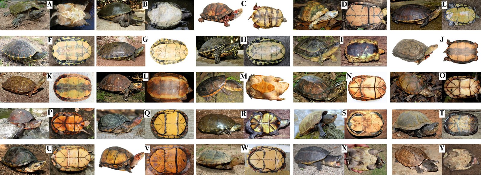
Figure 2. Photos of the continental turtles of southeastern Mexico. All photos (except when indicated, see Acknowledgments) by Eduardo Reyes-Grajales or John B. Iverson. A. Chelydra rossignonii, B. Dermatemys mawii, C. Terrapene mexicana, D. T. yucatana, E. Trachemys grayi grayi, F. T. venusta cataspila, G. T. v. iversoni, H. T. v. venusta, I. Rhinoclemmys areolata, J. R. pulcherrima incisa, K. R. p. pulcherrima, L. R. rubida rubida, M. Claudius angustatus, N. Kinosternon abaxillare, O. K. acutum, P. K. creaseri, Q. K. cruentatum, R. K. flavescens, S. K. herrerai, T. K. integrum, U. K. leucostomum, V. K. mexicanum, W. K. oaxacae, X. Staurotypus salvinii, Y. S. triporcatus.
Distributions of continental turtles of southeastern Mexico
In this section the abbreviations are: Ca = Campeche, Ch = Chiapas, Oa = Oaxaca, QR = Quintana Roo, Ta = Tabasco, Ve = Veracruz, Yu = Yucatán.
Chelydra rossignonii (Bocourt, 1868; Figs. 2A, 3A): along the Gulf of Mexico versant from the Jamapa River (Ve) to the Usumacinta River (Ta and Ch), including Laguna de Terminos (Ca). Other rivers include the Papaloapan, Coatzacoalcos (both in Oa and Ve), and lower Grijalva (Ch).
Dermatemys mawii Gray, 1847 (Figs. 2B, 3B): from the Jamapa River (Ve) to Champoton River (Ca) on the Gulf of Mexico versant, including the Usumacinta (Ca, Ch and Ta) and Lacantun Rivers (Ch). In Chetumal Bay (QR) the distribution extends to and beyond the Belize border.
Terrapene mexicana (Gray, 1849; Figs. 2C, 3C): from the Tamesi River to the Jamapa River, including the Tamiahua Lake area; on the Gulf of Mexico versant in Veracruz and northward into Tamaulipas.
Terrapene yucatana (Boulenger, 1895; Figs. 2D, 3C): most of the western Yucatán Peninsula (primarily Yucatán and Campeche), with rare and localized occurrences in the northern region of Quintana Roo.
Trachemys grayi grayi (Bocourt, 1868; Figs. 2E, 3D): from La Arena River (Oa) to the Suchiate River on the Pacific versant (Ch), and southward to El Salvador.
Trachemys venusta cataspila (Günther, 1885; Figs. 2F, 3D): from the Jamapa River to the Panuco River (both in Ve) on the Gulf of Mexico versant, and northward in Tamaulipas.
Trachemys venusta iversoni McCord, Joseph-Ouni, Hagen, and Blanck, 2010 (Figs. 2G, 3D): most of the northern portions of Yucatán and Quintana Roo.
Trachemys venusta venusta (Gray, 1856; Figs. 2H, 3D): from the Jamapa River (Ve) to the Champoton River (Ca) on the Gulf of Mexico versant, including the Usumacinta (Ca, Ch and Ta) and Lacantun Rivers (Ch). In Chetumal Bay (QR) the distribution continues across the border into Belize and Guatemala.
Rhinoclemmys areolata (Duméril and Bibron in Duméril and Duméril, 1851; Figs. 2I, 3E): from the Jamapa River eastward (Ve) on the Gulf of Mexico versant throughout the north portions of Oaxaca and Chiapas and extended across Tabasco and the Yucatán peninsula (Ca, Yu and QR), and into Guatemala and Belize.
Rhinoclemmys pulcherrima incisa (Bocourt, 1868; Figs. 2J, 3F): from the west portion of the Copalita River (Oa) to the Suchiate River (Ch) on the Pacific versant, and southeast to Nicaragua.
Rhinoclemmys pulcherrima pulcherrima (Gray, 1856; Figs. 2K, 3F): from the Tehuantepec River (Oa) westward on the Pacific versant to the Balsas River, Guerrero.
Rhinoclemmys rubida rubida (Cope, 1870; Figs. 2L, 3E): from the Ometepec River (Oa) to the Suchiate River (Ch) on the Pacific versant, including the Atoyac and Tehuantepec basins (both in Oa).
Claudius angustatus Cope, 1865 (Figs. 2M, 3G): from the Jamapa River (Ve) to the western and southern Yucatán peninsula on the Gulf of Mexico versant, including the Usumacinta (Ca, Ch and Ta) and Lacantun Rivers (Ch), and southward into Guatemala and Belize.
Kinosternon abaxillare Baur in Stejneger, 1925 (Figs. 2N, 3H): restricted to the Grijalva River basin in the Central Depression and Plateau of Chiapas.
Kinosternon acutum Gray, 1831 (Figs. 2O, 3H): from the Jamapa River (Ve) to the Champoton River (Ca) on the Gulf of Mexico versant, including the Papaloapan, Coatzacoalcos (both in Oa and Ve) and lower Grijalva Rivers (Ch), and Laguna de Terminos (Ca). Also found on the southern Yucatán peninsula (Ca and QR), northern Guatemala and Belize.
Kinosternon creaseri Hartweg, 1934 (Figs. 2P, 3H): from the Champoton River (Ca) across the Yucatán peninsula (QR and Yu).
Kinosternon cruentatum Duméril and Bibron in Duméril and Duméril, 1851 (Figs. 2Q, 3I): from the Pánuco River (Ve) across the Tabasco lowlands to the entire Yucatán Peninsula on the Gulf of Mexico versant and into Guatemala and Belize.
Kinosternon flavescens Agassiz, 1857 (Figs. 2R, 3J): in southeastern Mexico it is restricted to the Panuco River basin (Ve) but ranges north across the Great Plains of the USA.
Kinosternon herrerai Stejneger, 1925 (Figs. 2S, 3K): from the Jamapa to the Panuco River (both in Ve) and northward on the Gulf of Mexico versant.
Kinosternon integrum Le Conte, 1854 (Figs. 2T, 3J): in southern Mexico from the Atoyac (Oa and Ve) and Tlapaneco River basins westward (Oa).
Kinosternon leucostomum Duméril and Bibron in Duméril and Duméril, 1851 (Figs. 2U, 3K): from the Jamapa River (Ve) to the Champoton River (Ca) on the Gulf of Mexico versant, including the Usumacinta (Ca, Ch and Ta) and Lacantun rivers (Ch). Also found from Chetumal Bay through eastern Quintana Roo, and southward through Central America.
Kinosternon mexicanum Le Conte, 1854 (Figs. 2V, 3J): restricted to the Pacific versant from the Tehuantepec River (Oa) to the Suchiate River (Ch), and southeast to El Salvador.
Kinosternon oaxacae Berry and Iverson, 1980 (Figs. 2W, 3J): restricted to the Ometepec, La Arena, Colotepec and Copalita River basins on the Pacific versant in Oaxaca; also, westward into Guerrero.
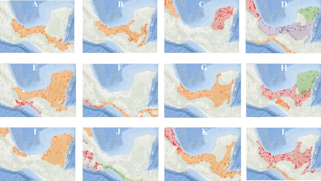
Figure 3. Distribution maps of the continental turtles of southern Mexico. The shaded color represents the distribution of each taxon (taken from TTWG, 2025). Maps with 2 or more taxa present dots and shade ranges with similar colors, and maps with a single taxa dots and shade ranges are orange. A. Chelydra rossignonii, B. Dermatemys mawii, C. Terrapene mexicana (orange), T. yucatana (red), D. Trachemys grayi grayi (orange), T. venusta cataspila (red), T. v. iversoni (green), T. v. venusta (purple), E. Rhinoclemmys areolata (orange), R. rubida rubida (red), F. R. pulcherrima incisa (orange), R. p. pulcherrima (red), G. Claudius angustatus, H. Kinosternon abaxillare (orange), K. acutum (red), K. creaseri (green), I. K. cruentatum (orange), J. K. flavescens (orange), K. integrum (red), K. mexicanum (green), K. oaxacae (purple) K. K. herrerai (red), K. leucostomum (orange), L. Staurotypus salvinii (orange), S. triporcatus (red). Maps by Eduardo Reyes-Grajales.
Staurotypus salvinii Gray, 1864 (Figs. 2X, 3L): from the Copalita River (Oa) to the Suchiate River (Ch) on the Pacific versant, and southeast to El Salvador.
Staurotypus triporcatus (Wiegmann, 1828; Figs. 2Y, 3L): from the Jamapa River (Ve) to Campeche state on the Gulf of Mexico versant, including the Usumacinta (Ca, Ch and Ta) and Lacantun River (Ch). Also, in southern Quintana Roo to Chetumal Bay and into Guatemala, Belize and northwestern Honduras. Insertar fig 3:12cm
There was a wide range of conservation status for most of the native turtle taxa under national and international criteria. For example, the Mexican Government list (NOM-059 list; Semarnat, 2010) includes 16 species (64% of all turtle taxa found in southeastern Mexico), the IUCN Red List includes 18 (72%), and 20 are CITES listed (80%; Table 3). The turtles listed by NOM-059 and IUCN Red List as most threatened are D. mawii, C. angustatus, and those within the genus Terrapene (Table 3). However, the taxa whose conservation status is totally unknown includes all species in the genus Trachemys (Table 3). The average EDGE score for southeastern Mexican turtle taxa was 4.41 with a minimum value of 3.67 (K. creaseri, K. flavescens, and K. integrum), and a maximum of 7.15 (D. mawii) (Table 3).
Discussion
This is the first dichotomous key based on external characteristics to consider all native continental turtles that are distributed in southeastern Mexico, in accordance with advances in turtle taxonomy. Other dichotomous keys, although effective, are based on the review of internal characteristics that require the sacrifice of the organisms —e.g., for cranial measurements (Legler & Vogt, 2013). These criteria may not be useful when carrying out population ecology studies, or when required in forensic procedures, as for the identification of confiscated turtles. The inclusion of a Spanish translation may facilitate the work of early-career professionals and local authorities in the preparation of expert reports on seized specimens, contributing to a more accurate assessment of the extent of illegal trade affecting certain taxa. Generally, when there are national reports of seizures involving mud turtles, this is limited to filing a report at the genus level (Profepa, 2020).
According to our results, southeastern Mexico supports 3/4 of the families —and more than half of the genera— found nationwide in Mexico (Table 2). These findings highlight southeastern Mexico as a region of high importance for the composition of land and freshwater turtles at the national level. This fact is consistent with studies focused on analyzing the composition of the Mexican herpetofauna (Flores-Villela & García-Vazquez, 2014; Johnson et al., 2017; Ramírez-Bautista et al., 2023). In addition to this, Oaxaca, Chiapas, and Veracruz stand out as the states with the highest species richness and/or endemism, respectively. These 3 states are located within the region considered the richest in total herpetofauna, a result of complex orography, diverse habitats and environments, and the biogeographic history of Mexico (Ramírez-Bautista et al., 2023).
Previously published checklists of reptile diversity in Mexico often included taxonomic and distributional inconsistencies for turtles, possibly due to the disposition of the taxonomic status at that time (e.g., Flores-Villela & García-Vazquez, 2014; Hernández-Ordoñez et al., 2015; Johnson et al., 2015; Wilson et al., 2013). For example, Johnson et al. (2015) reported the presence of T. ornata in Chiapas, but according to the TTWG (2021, 2025) this species occurs only in western Mexico, from Culiacan, Sinaloa to Puerto Vallarta, Jalisco. Likewise, R. areolata and C. serpentina have been reported from the southeastern part of the Lacandona rainforest, Chiapas (Hernández-Ordoñez et al., 2015). However, experts agree that there is no evidence for native populations of R. areolata in that region (TTWG, 2021, 2025). Velázquez-Nucamendi et al. (2021) suggested that the records might involve animals transported from Tabasco to this region of Chiapas. Furthermore, the closely related C. serpentina and C. rossignonii are commonly confused in southeastern Mexico, despite the former species being found only in the United States and Canada (TTWG, 2021, 2025).
It is important to note that the Berlandier’s tortoise (Testudinidae: Gopherus berlandieri) has been reported from the northern portion of Veracruz in recent checklists (Torres-Hernández et al., 2021; Vásquez-Cruz et al., 2021) and in virtual repositories (GBIF, 2024; iNaturalist, 2024; SNIB-Conabio, 2024). However, the inclusion of this turtle in these reports is not confirmed by collection data, and in the case of virtual repositories, it is based on individuals in captivity near the state border with Tamaulipas, where G. berlandieri is known to occur naturally. As no wild populations have been reported, and no wild individuals have been formally collected in the northern portion of Veracruz, we do not consider this species native to Veracruz. However, this issue needs to be addressed in the future to clarify the total richness of continental turtles in southeastern Mexico.
Southeastern Mexico has been categorized globally as an area with high to moderate endemism (Ennen et al., 2020). Our data indicates that this region contains 33% of the endemic continental turtle taxa at the national level within the genera Terrapene, Trachemys, Rhinoclemmys, and Kinosternon (Table 3). However, there are suggestions that in this region the probability remains high for potential new taxonomic discoveries or upgrades from subspecies to species, especially within Trachemys and Kinosternon, 2 genera that have been poorly studied in Mexico (Flores-Villela & García-Vázquez, 2014; Legler & Vogt, 2013). The T. venusta complex has historically presented many inconsistencies in its taxonomic relationships. Despite prominent color pattern differences among species, genetic divergences within this complex are shallow, and the taxonomic diversity of each species with several currently recognized subspecies could be overestimated (Fritz et al., 2011, 2023; Parham et al., 2013; Seidel & Ernst, 2017). Another scientific priority is to clarify the genetically distinct group of D. mawii located in the Papaloapan River in Veracruz (González-Porter et al., 2011), and into the Lacandona rainforest (Martínez Gómez et al., 2017).
Historically, turtles in southeastern Mexico have been widely exploited at unsustainable rates, resulting in negative repercussions on their populations and pushing some species to the brink of near local extinctions (Legler & Vogt, 2013). Examples include C. angustatus and D. mawii, both recognized as most threatened by national criteria (Table 3). For the first species, in a study conducted in Lerdo de Tejada, Veracruz (Mexico), Espejel-González (2004) reported a capture of 254 individuals. However, due to the high rates of extraction per year (Espejel-González, 2004), Reynoso et al. (2016) found no individuals in the same locality. For D. mawii in the Lacandona rainforest (Chiapas), a systematic evaluation that started in the 1980s and concluded 20 years later inferred a reduction of ~ 80% of the native population in the area (Guichard-Romero, 2006; Legler & Vogt, 2013). Other current events that provide a glimpse of the crisis facing Mexican turtles include 2 trade confiscations in 2020. In just 2 seizures, approximately 30,000 Mexican turtles were confiscated, mainly Trachemys, Kinosternon, Claudius, and Staurotypus (Profepa, 2020; Excelsior, 2020).
We found that D. mawii, T. mexicana, and T. yucatana were the only species in which their risk categories were consistent under national and international criteria. For the remainder of the turtles distributed in southeastern Mexico, these categorizations were inconsistent or nonexistent (Table 3). The genus Trachemys is the one that is not under any national or international protection criteria (Table 3). The absence of protection criteria does not indicate a lesser concern for the conservation of these turtles, but rather a potential neglect of an approach to diagnose the conservation status through their distribution, even though these turtles are highly demanded for local consumption and the illegal pet trade (Beauregard-Solís et al., 2010; Profepa, 2020; Velázquez-Nucamendi et al., 2021). One main problem for the conservation of turtles in Mexico is the lack of concordance between the lists issued by the national Government and those by international organizations (Macip-Ríos et al., 2015). This leads to confusion by the Mexican public administration regarding the data available for decisions related to management and permitting, especially for species poor studied and highly demanded as Trachemys and Kinosternon (Macip-Ríos et al., 2015; Profepa, 2020).
Mexico is an active country in the trade of wild species. Just in the period 2007-2011, Mexico was the second-largest exporter worldwide, with approximately 750,000 specimens of live reptiles removed, of which continental turtles stood out (Semarnat, 2012). Therefore, agreement between national and international standards is a high priority to conserve Mexican turtle species. More research and data are needed on least Rhinoclemmys, K. cruentatum, K. herrerai, K. leucostomum, K. oaxacae, K. mexicanum, and S. salvinii. The need for updates in national and international legal regulations is recognized as essential to the protection of the different species of turtles that are distributed in southeastern Mexico. We encourage the assessment of population trends and potential threats to provide a more comprehensive conservation status for these turtles under national and international criteria.
The information provided in this work should help to improve and focus future research and conservation in southeastern Mexico. However, we recognize that more information is required on the population status of the turtles in each state to face the new challenges that we need to consider for their conservation. Indeed, addressing the remaining gaps in the distribution and systematics of certain turtle species would be a valuable avenue for future research. Continued efforts to enhance our understanding of these aspects will contribute to more accurate assessments of conservation status. Finally, we encourage the resolution of the discrepancies between international and Mexican conservation priorities to ensure the protection of the turtles that occur in this region. Aligning priorities will help create more unified and impactful strategies, ensuring better protection for these turtles and their habitats (Macip-Ríos et al., 2015). This underscores the importance of international collaboration and coordination to address conservation challenges comprehensively.
Acknowledgments
Fieldwork was conducted under the Mexican Federal Government permit numbers: SGPA/DGVS/01156/19 and SGPA/DGVS/06570/21 issued by Semarnat. We thank the authorities of the Áreas Naturales y Vida Silvestre from SEMAHN for providing essential information on turtle locations; Carlos A. Guichard Romero and Antonio Ramirez for providing access to the ZooMAT facilities; Antonio Muñoz Alonso for providing access to the reptile collection from ECOSUR, and Anders G. J. Rhodin for providing all Mexican turtle localities from the Turtle Taxonomy Working Group’s distributional database (TTWG 2021, 2025). For photographs in Fig. 2, we thank Ernesto Eduardo Perera Trejo (A, general view and plastron), Julio Gonzalez (C, plastron), Mike Jones (D and P, general view and plastron), Taggert Butterfield (L plastron), Alejandra Monsivais (K general view and plastron), Antonio Ramírez (M, general view), and Erasmo Cázares (S, general view and plastron). Anders G. J. Rhodin, Peter Paul van Dijk, Oscar Flores-Villela, Taggert Butterfield, Jacobo Reyes-Velasco and Donald McKnight made important comments to improve this manuscript. We thank the Turtle Survival Alliance, Mohamed bin Zayed Species Conservation Fund (242536595), Turtle Conservation Fund, Chelonian Research Foundation (TCF-0790), and Turtle Taxonomy Fund for their support during field work and laboratory analysis. Finally, ERG is grateful to the scholarship “Becas de Preparación de Posgrado” from El Colegio de la Frontera Sur for support during the writing of this work.
References
Auth, D. L., Smith, H. M., Brown, B. C., & Lintz, D. (2000). A description of the Mexican amphibian and reptile collection of the Strecker Museum. Bulletin of the Chicago Herpetological Society, 35, 65–85.
Barão-Nóbrega, J. A. L., Nahuat-Cervera, P. E., Avella, I., Capehart, G., Garcia, B., Oakley, J. et al. (2022). Herpetological diversity in Calakmul, Campeche, Mexico: species list with new distribution notes. Revista Mexicana de Biodiversidad, 93, e933927. https://doi.org/10.22201/ib.20078706e.2022.93.3927
Barragán-Vázquez, M. D. R., Ríos-Rodas, L., Fucsko, L. A., Mata-Silva, V., Porras, L. W., Rocha, A. et al. (2022). The herpetofauna of Tabasco, Mexico: composition, distribution, and conservation status. Amphibian and Reptile Conservation, 16, 1–61.
Beauregard-Solís, G., Zenteno-Ruiz, C., Armijo-Torres, R., & Guzmán-Juárez, E. (2010). Las tortugas de agua dulce: patrimonio zoológico y cultural de Tabasco. Kuxulkab´, 17, 5–19.
Calderón, R., Cedeño-Vázquez, J. R., & Pozo, C. (2003). New distributional records for amphibians and reptiles from Campeche, Mexico. Herpetological Review, 34, 269–272.
Casas-Andreu, G., Méndez-De la Cruz, F. R., & Camarillo, J. L. (1996). Anfibios y reptiles de Oaxaca. Lista, distribución y conservación. Acta Zoológica Mexicana, 69, 1–35. https://doi.org/10.21829/azm.1996.69691928
Cázares-Hernández, E. (2015). Guía de las tortugas dulceacuícolas de Veracruz. Zongolica, Veracruz: Instituto Tecnológico Superior de Zongolica.
Charruau, P., Morales-Garduza, M. A., López-Luna, M. A., Reyes-
Trinidad, J. G., Ramírez-Pérez, M. A., López-Hernández, J. A. et al. (2023). Herpetofauna de los humedales de la laguna de Chaschoc, Tabasco, México. Revista Latinoamericana de Herpetología, 6, 75–92. https://doi.org/10.22201/fc.25942158e.2023.2.616
Chrapliwy, P. S. (1956). Extensions of known range of certain amphibians and reptiles of Mexico. Herpetologica, 12, 121–124.
CITES (Convention on International Trade in Endangered Species of Wild Fauna and Flora). (2024). The CITES Appendices, 2024. Retrieved April 7, 2023, from: https://cites.org/eng
Conabio (Comisión Nacional para el Conocimiento y Uso de la Biodiversidad). (2024). Comisión Nacional para el Conocimiento y Uso de la Biodiversidad. Retrieved April 7, 2024, from: https://www.gob.mx/conabio
Contreras-Balderas, S., Ruiz-Campos, G., Schmitter-Soto, J. J., Díaz-Pardo, E., Contreras-Macbeath, T., Medina-Soto, M. et al. (2008). Freshwater fishes and water status in México: a country-wide appraisal. Aquatic Ecosystem Health and Management, 11, 246–256.
Díaz-Gamboa, L., May-Herrera, D., Gallardo-Torres, A., Cedeño-Vázquez, R., González-Sánchez, V., Chiappa-Carrara, X. et al. (2020). Catálogo de reptiles de la península de Yucatán. Mérida, Yucatán: Escuela Nacional de Estudios Superiores Unidad Mérida, UNAM.
Edwards, T., Karl, A. E., Vaughn, M., Rosen, P. C., Torres, C. M., & Murphy, R.W. (2016). The Desert Tortoise trichotomy: Mexico hosts a third, new sister-species of tortoise in the Gopherus morafkai–G. agassizii group. Zookeys, 562, 131–158. https://doi.org/10.3897/zookeys.562.6124
Ennen, J. R., Agha, M., Sweat, S. C., Matamoros, W. A., Lovich, J. E., Rhodin, A. G. J. et al. (2020). Turtle biogeography: global regionalization and conservation priorities. Biological Conservation, 241, 108323. https://doi.org/10.1016/j.biocon.2019.108323
Ernst, C. H. (1978). A revision of the Neotropical turtle genus Callopsis (Testudines: Emydidae: Batagurinae). Herpetologica, 34, 113–134.
Espejel-González, V. E. (2004). Aspectos biológicos del manejo del chopontil, Claudius angustatus (Testudines: Staurotypinae) (M. Sc. Thesis). Universidad Nacional Autónoma de México, Xalapa, Veracruz.
EXCELSIOR. (2020). Estos son los animales rescatados tras decomiso histórico en Iztapalapa. Retrieved April 7, 2023, from: https://www.excelsior.com.mx/comunidad/estos-son-los-animales-rescatados-tras-decomiso-historico-en-iztapa
lapa/1419311
Ferreira-García, M. E., & Canseco-Márquez, L. (2006). Estudio de la herpetofauna del Monumento Natural Yaxchilán, Chiapas, México. In A. Ramírez-Bautista, L. Canseco-Máquez, & F. Mendoza-Quijano (Eds.), Inventarios herpetofaunísticos de México: avances en el conocimiento de su biodiversidad (pp. 293–310). México D.F.: Sociedad Herpetológica Mexicana, A.C.
Flores-Villela, O., & García-Vázquez, U. O. (2014). Biodiversidad de reptiles en México. Revista Mexicana de Biodiversidad, 85 (Suplem.), S467–S475. https://doi.org/10.7550/rmb.43236
Fritz, U., Kehlmaier, C., Scott, R. J., Fournier, R., McCranie, J. R., & Gallego-García, N. (2023). Central American Trachemys revisited: new sampling questions current understanding of taxonomy and distribution (Testudines: Emydidae). Vertebrate Zoology, 73, 513–523. https://doi.org/10.3897/vz.73.e104438
Fritz, U., Stuckas, H., Vargas-Ramírez, M., Hundsdöfer, A. K., Maran, J., & Päckert, M. (2011). Molecular phylogeny of Central and South American slider turtles: implications for biogeography and systematics (Testudines: Emydidae: Trachemys). Journal of Zoological Systematics and Evolutionary Research, 50, 125–136. https://doi.org/10.1111/j.1439-0469.2011.00647.x
GBIF (Global Biodiversity Information Facility). (2024). Retrieved April 7, 2023, from: https://www.gbif.org/
González-Porter, G. P., Hailer, F., Flores-Villela, O., García-Anleu, R., & Maldonado, J. E. (2011). Patterns of genetic diversity in the critically endangered Central American river turtle: human influence since the Mayan age? Conservation Genetics, 12, 1229–1242. https://doi.org/10.1007/s10592-011-0225-x
González-Sánchez, V. H., Johnson, J. D., García-Padilla, E., Mata-Silva, V., DeSantis, D. L., & Wilson. L.D. (2017). The herpetofauna of the Mexican Yucatán Peninsula: composition, distribution, and conservation. Mesoamerican Herpetology, 4, 264–380.
Guichard-Romero, C. A. (2006). Situación actual de las poblaciones de tortuga blanca (Dermatemys mawii) en el sureste de México (Informe final del Proyecto AS003-Conabio). Mexico City: Comisión Nacional para el Conocimiento y Uso de la Biodiversidad.
Gumbs, R., Gray, C. L., Wearn, O. R., & Owen, N. R. (2018). Tetrapods on the EDGE: Overcoming data limitations to identify phylogenetic conservation priorities. Plos One, 13, e0194680. https://doi.org/10.1371/journal.pone.0194680
Hernández-Ordoñez, O., Arroyo-Rodríguez, V., González-Hernández, A., Russildi, G., Luna-Reyes, R., Martínez-Ramos, M. et al. (2015). Extensión del área de distribución de anfibios y reptiles en la parte sureste de la selva Lacandona, México. Revista Mexicana de Biodiversidad, 86, 457–468. https://doi.org/10.1016/j.rmb.2015.04.005
Hernández-Ordóñez, O., Martínez-Ramos, M., Arroyo-Rodríguez, V., González-Hernández, A., González-Zamora, A., Zárate, D. A. et al. (2014). Distribution and conservation status of amphibian and reptile species in the Lacandona rainforest, Mexico: an update after 20 years of research. Tropical Conservation Science, 7, 1–25. https://doi.org/10.1177%2F194008291400700101
Huidobro, L., Morrone, J. J., Villalobos, J. L., & Álvarez, F. (2006). Distributional patterns of freshwater taxa (fishes, crustaceans, and plants) from the Mexican transition zone. Journal of Biogeography, 33, 731–741. https://doi.org/10.1111/j.1365-2699.2005.01400.x
Hurtado-Gómez, J. P., Vargas-Ramírez, M., Iverson, J. B., Joyce, W., Mccranie, J. R., & Fritz, U. 2024. Diversity and biogeography of South American Mud Turtles elucidated by multilocus DNA sequencing (Testudines: Kinosternidae). Molecular Phylogenetics and Evolution, 197, 108083. https://doi.org/10.1016/j.ympev.2024.108083
Hutchison, J. H., & Bramble, D. M. (1981). Homology of the plastral scales of the Kinosternidae and related turtles. Herpetologica, 37, 73–85.
iNaturalist. (2024). iNaturalist. Retrieved June 6, 2024, from: https://www.inaturalist.org/
IUCN (International Union for the Conservation of Nature). 2024. IUCN Red List of Threatened Species. Retrieved June 6, 2024, from: http://www.iucnredlist.org
INEGI (Instituto Nacional de Estadística y Geografía). (2021). Instituto Nacional de Estadística y Geografía. Retrieved March 3, 2021: https://www.inegi.org.mx/
Iverson, J. B., & Berry, J. F. (2024). Morphometric variation in the Red-cheeked Mud Turtle (Kinosternon cruentatum) and its taxonomic significance. Chelonian Conservation and Biology, 23, 13–22. https://doi.org/10.2744/CCB-1589.1
Iverson, J. B., Le, M., & Ingram, C. (2013). Molecular phylogenetics of the mud and musk turtle family Kinos-
ternidae. Mollecular Phylogenetics and Evolution, 69, 929–939. https://doi.org/10.1016/j.ympev.2013.06.011
Johnson, J. D., Mata-Silva, V., García-Padilla, E., & Wilson, L. D. (2015). The herpetofauna of Chiapas, Mexico: compo-
sition, distribution, and conservation. Mesoamerican Herpetology, 2, 272–329.
Johnson, J. D., Wilson, L. D., Mata-Silva, V., García-Padilla, E., & DeSantis, D. L. (2017). The endemic herpetofauna of Mexico: organisms of global significance in severe peril. Mesoamerican Herpetology, 4, 544–620.
Lee, J. C. (1996). The amphibians and reptiles of the Yucatán Peninsula. Ithaca: Cornell University Press.
Legler, J. M. (1990). The genus Pseudemys in Mesoamerica: taxonomy, distribution, and origins. In J. W. Gibbons (Ed.), Life history and ecology of the slider turtle (pp. 82–105). Washington D.C: Smithsonian Institution Press.
Legler, J. M., & Vogt, R. C. (2013). The turtles of Mexico: land and freshwater forms. Berkeley, California: University of California Press.
Leopold, A. S. (1950). Vegetation zones of Mexico. Ecology, 31, 507–518.
Loc-Barragán, J. A., Reyes-Velasco, J., Woolrich-Piña, G. A., Grünwald, C. T., Venegas-de Anaya, M., Rangel-Mendoza, J. et al. (2020). A new species of mud turtle of genus Kinosternon (Testudines: Kinosternidae) from the Pacific coastal plain of northwestern Mexico. Zootaxa, 4885, 509–529. https://doi.org/10.11646/zootaxa.4885.4.3
López-Luna, M. A., Cupul-Magaña, F. G., Escobedo-Galván, A. H., Gonzáles-Hernández, A. J., Centenero-Alcalá, E., Rangel-Mendoza, J. A. et al. (2018). A distinctive new species of mud turtle from western Mexico. Chelonian Conservation and Biology, 17, 2–13. https://doi.org/10.2744/CCB-1292.1
Luna-Reyes, R., Canseco-Márquez, L., & Hernández-García, E. (2013). Los reptiles. In A. Cruz-Angón, E. D. Melgarejo, F. Camacho-Rico y K. C. Nájera-Cordero (Ed.), La biodiversidad en Chiapas, Estudio de Estado (pp.319–328). México D.F.: Comisión Nacional para el Conocimiento y Uso de la Biodiversidad/ Gobierno del Estado de Chiapas.
Macip-Ríos, R., Ontiveros, R., López-Alcaide, S., & Casas-Andreu, G. (2015). The conservation status of the freshwater and terrestrial turtles of Mexico: A critical review of biodiversity conservation strategies. Revista Mexicana de Biodiversidad, 86, 1048–1057. https://doi.org/10.1016/j.rmb.2015.09.013
Martin, B. T., Bernstein, N. P., Birkhead, R. D., Koukl, J. F., Mussmann, S. M., & Placyk, J. S. (2013). Sequence-based molecular phylogenetics and phylogeography of the American box turtles (Terrapene spp.) with support from DNA barcoding. Molecular Phylogenetics and Evolution, 68, 119–134. https://doi.org/10.1016/j.ympev.2013.03.006
Martínez-Gómez, J. (2017). Sistemática molecular e historia evolutiva de la Familia Dermatemydidae en Mesoamérica (Bachelor Thesis). Universidad de Ciencias y Artes de Chiapas. Chiapas, México.
Mata-Silva, V., García-Padilla, E. L., Rocha, A., Desantis, D. L., Johnson, J. D., Ramírez-Bautista, A. et al. (2021). A reexamination of the herpetofauna of Oaxaca, Mexico: composition update, physiographic distribution, and conservation commentary. Zootaxa, 4996, 201–252. https://doi.org/10.11646/zootaxa.4996.2.1
Mata-Silva, V., Johnson, J. D., Wilson, L. D., & García-Padilla, E. (2015). The herpetofauna of Oaxaca, Mexico: composition, physiographic distribution, and conservation status. Mesoamerican Herpetology, 2, 6–62.
McCord, W. P., Joseph-Ouni, M., Hagen, C., & Blanck, T. (2010). Three new subspecies of Trachemys venusta (Testudines: Emydidae) from Honduras, northern Yucatán (Mexico), and Pacific coastal Panama. Reptilia, 71, 39–49.
McCord, R. D. (2016). What is Kinosternon arizonense? Historical Biology, 28, 310–315. https://doi.org/10.1080/08912963.2015.1053879
Moldowan, P. D., Brooks, R. J., & Litzgus, J. D. (2015). Turtles with “teeth”: beak morphology of Testudines with a focus on the tomiodonts of Painted Turtles (Chrysemys spp.). Zoomorphology, 35, 121–135. https://doi.org/10.1007/s00435-015-0288-1
Moreno-Avendaño, V., & Reyes-Grajales, E. (2022). Distribution. Central Chiapas Mud Turtle. Kinosternon abaxillare. Herpetological Review, 53, 261.
Murphy, R. W., Berry, K. H., Edwards, T., Leviton, A. E., Lathrop, A., & Riedle, J. D. (2011). The dazed and confused identity of Agassiz’s land tortoise, Gopherus agassizii (Testudines, Testudinidae) with the description of a new species, and its consequences for conservation. Zookeys, 113, 39–71. https://doi.org/10.3897/zookeys.113.1353
Muñoz-Alonso, L. A., Rodiles-Hernández, R., López-León, N. P., González-Navarro, A., Chau-Cortés, A. M., & Nieblas-Camacho, J. A. (2018). Diversidad de la herpetofauna en la cuenca del Usumacinta, México. Revista Mexicana de Biodiversidad, 89 (Suplem.), 79–99. https://doi.org/10.22201/ib.20078706e.2018.0.2447
Ortiz-Medina, J. A., Cabrera-Cen, D. I., Nahuat-Cervera, P. E., & Chablé-Santos, J. B. (2020). New distributional records for the herpetofauna of Campeche and Yucatán, Mexico. Herpetological Review, 51, 83–87.
Parham, J. F., Papenfuss, T. J., van Dijk, P. P., Wilson, B. S., Marte, C., Rodríguez-Schettino, L. et al. (2013). Genetic introgression and hybridization in Antillean freshwater turtles (Trachemys) revealed by coalescent analyses of mitochondrial and cloned nuclear markers. Molecular Phylogenetics and Evolution, 67, 176–187. https://doi.org/10.1016/j.ympev.2013.01.004
Profepa (Procuraduría Federal de Protección al Ambiente). 2020. Profepa asegura precautoriamente más de 15 mil tortugas que pretendían exportarse de manera ilegal a China. Retrieved March 3, 2021: https://www.gob.mx/profepa/prensa/profepa-asegura-precautoriamente-mas-de-15-mil-tortugas-que-pretendian-exportarse-de-manera-ilegal-a-china?idiom=es
Quiroz-Martínez, B., Álvarez, F., Espinosa, H., & Salgado-Maldonado, G. (2014). Concordant biogeographic patterns among multiple taxonomic groups in the Mexican freshwater biota. Plos one, 9, e105510. https://doi.org/10.1371/journal.pone.0105510
Ramírez-Bautista, A., Torres-Hernández, L. A., Cruz-Elizalde, R., Berriozábal-Islas, C., Hernández-Salinas, U., Wilson, L. D. et al. (2023). An updated list of the Mexican herpetofauna: with a summary of historical and contemporary studies. Zookeys, 1166, 287–306. https://doi.org/10.3897/zookeys.1166.86986
Ramírez-González, C. G., & Canseco Márquez, L. (2015). Chelydra rossignonii, confirmación de su presencia en el estado de Oaxaca. Revista Mexicana de Biodiversidad, 86, 832–834. https://doi.org/10.1016/j.rmb.2015.05.007
Reynoso-Rosales, V. H., Vázquez-Cruz, M. L., & Rivera-Arroyo, R. C. (2016). Estado de conservación, uso, gestión, comercio y cumplimiento de los criterios de inclusión a los Apéndices de la CITES para las especies Claudius
angustatus y Staurotypus triporcatus. Mexico City: Conabio-CITES.
Ríos-Solís, J. A., Lavariega, M. C., García-Padilla, E., & Mata-Silva, V. (2021). Noteworthy records of freshwater turtles in Oaxaca, Mexico. Revista Latinoamericana de Herpetología, 4, 184–191.
Semarnat (Secretaría de Medio Ambiente y Recursos Naturales). (2010). Norma Oficial Mexicana NOM-059-SEMARNAT-2010, Protección ambiental – Especies nativas de México de flora y fauna silvestres – Categorías de riesgo y especificaciones para su inclusión, exclusión o cambio – Lista de especies en riesgo. Diario Oficial de la Federación. 30 de diciembre de 2010, Segunda Sección, México.
Semarnat (Secretaría de Medio Ambiente y Recursos Naturales). (2012). Informe anual PROFEPA 2012. México D.F.: Semarnat.
Semarnat (Secretaría de Medio Ambiente y Recursos Naturales). (2025). Proyecto de Norma Oficial Mexicana PROY-NOM-059-SEMARNAT-2025, Protección ambiental – Especies nativas de México de flora y fauna silvestres – Categorías de riesgo y especificaciones para su inclusión, exclusión o cambio – Lista de especies en riesgo. Diario Oficial de la Federación. 14 de abril de 2025, Segunda Sección, México.
Seidel, M. E., & Ernst, C. H. (2017). A systematic review of the turtle family Emydidae. Vertebrate Zoology, 67, 1–122. https://doi.org/10.3897/vz.67.e31535
Spencer, R. J., Van Dyke, J. U., & Thompson, M. B. (2017). Critically evaluating best management practices for preventing freshwater turtle extinctions. Conservation Biology, 6, 1340–1349. https://doi.org/10.1111/cobi.12930
Spinks, P. Q., Thomson, R. C., Gidiş, M., & Shaffer, H. B. (2014). Multilocus phylogeny of the New-World mud turtles (Kinosternidae) supports the traditional classification of the group. Molecular Phylogenetics and Evolution, 76, 254–260. https://doi.org/10.1016/j.ympev.2014.03.025
Torres-Hernández, L. A., Ramírez-Bautista, A., Cruz-Elizalde, R., Hernández-Salinas, U., Berriozábal-Islas, C., DeSantis, D. L. et al. (2021). The herpetofauna of Veracruz, Mexico: composition, distribution, and conservation status. Amphibian and Reptile Conservation, 15, 72–155.
Turtle Conservation Coalition (TCC: Stanford, C. B., Rhodin, A. G. J., van Dijk, P. P., Horne, B. D., Blanck, T., Goode, E. V., Hudson, R., Mittermeier, R. A., Currylow, A., Eisemberg C. et al.). (2018). Turtles in Trouble: The World’s 25+ Most Endangered Tortoises and Freshwater Turtles—2018. Ojai, California: IUCN SSC Tortoise and Freshwater Turtle Specialist Group, Turtle Conservancy, Turtle Survival Alliance, Turtle Conservation Fund, Chelonian Research Foundation, Conservation International, Wildlife Conservation Society, and Global Wildlife Conservation.
Turtle Taxonomy Working Group (TTWG: Rhodin, A. G. J., Iverson, J. B., Bour, R., Fritz, U., Georges, A., Shaffer, H. B., & van Dijk, P. P.). (2021). Turtles of the World: annotated checklist and atlas of taxonomy, synonymy, distribution, and conservation status. 9th Edition. Chelonian Research Monographs 8. Rochester, NY.
Turtle Taxonomy Working Group (TTWG: Rhodin, A. G. J., Iverson, J. B., Fritz, U., Gallego-García, N., Georges, A., Ihlow, F., Shaffer, H. B., & van Dijk, P. P.). (2025). Turtles of the World: Annotated Checklist and Atlas of Taxonomy, Synonymy, Distribution, and Conservation Status (10th Ed.). Chelonian Research Monographs 9.
Vásquez-Cruz, V., Cazares-Hernández, E., Reynoso-Martínez, A., Kelly-Hernández, A., Fuentes-Moreno A., & Lara-Hernández, F. A. (2021). New distributional records of freshwater turtles from west-central Veracruz, Mexico. Reptiles and Amphibians, 28, 146–151. https://doi.org/10.17161/randa.v28i1.15373
Velázquez-Nucamendi, I. A., García-del Valle, Y., Reyes-Grajales, E., Sánchez-Cortés, M. S., & Ruan-Soto, F. (2021). Usos, prácticas y conocimiento local sobre las tortugas continentales (Testudines: Cryptodira) de la comunidad de Playón de la Gloria, Chiapas, México. Revista de Etnobiología, 19, 46–61.
Wilson, L. D., Mata-Silva, V., & Johnson, J. D. (2013). A conservation reassessment of the reptiles of Mexico based on the EVS measure. Amphibian and Reptile Conservation, 7, 1–47.
Winokur, R. M. (1982). Integumentary appendages of chelonians. Journal of Morphology, 172, 59–74. https://doi.org/10.1002/jmor.1051720106

Contribution to the systematic value of the leaf trichomes in the Cordiaceae (Boraginales)
Hamid Nazari a, Farrokh Ghahremaninejad b, *
a Bu-Ali Sina University, Department of Biology, 6517838695, Hamedan, Iran
b Kharazmi University, Faculty of Biological Sciences, Department of Plant Sciences, 4911-15719, Tehran, Iran
*Corresponding author: fgh@khu.ac.ir (F. Ghahremaninejad)
Received: 07 November 2024; accepted: 21 March 2025
Abstract
Leaf trichomes are vital for plant physiology, defense, and ecological interactions. This study utilized scanning electron microscopy to examine the leaf trichomes of 7 species in the family Cordiaceae, including 5 species from the genus Cordia and 2 from Varronia. Various types of trichomes, including glandular, non-glandular, and stellate, were observed. Our findings highlight differences in trichome types, density, and distribution both within and between genera. This research enhances the understanding of anatomical diversity and the significance of leaf trichomes in Cordiaceae, providing a foundation for future studies in plant biology. The high diversity of trichome structure in the studied species indicates their importance for their classification. Therefore, the results of this study provide a useful insight into the diversity of trichomes and their potential as a taxonomic tool.
Keywords: Indumentum; Glandular; Non-glandular; Stellate trichomes; Taxonomy
Resumen
Los tricomas de las hojas son vitales para la fisiología, la defensa y las interacciones ecológicas de las plantas. Este estudio utilizó microscopía electrónica de barrido para examinar los tricomas de las hojas de 7 especies de la familia Cordiaceae; se incluyeron 5 de los géneros Cordia y 2 de Varronia. Se observaron varios tipos de tricomas, incluidos glandulares, no glandulares y estrellados. Nuestros hallazgos resaltan las diferencias en los tipos de tricomas, la densidad y la distribución tanto dentro como entre géneros. Esta investigación mejora la comprensión de la diversidad anatómica, resalta la importancia de los tricomas de las hojas en Cordiaceae y proporciona una base para futuros estudios en biología vegetal. La gran diversidad de la estructura de los tricomas en las especies estudiadas indica su importancia para su clasificación. Por lo tanto, los resultados de este estudio proporcionan una buena visión de la diversidad de tricomas y su potencial como herramienta taxonómica.
Palabras clave: Indumento; Glandular; No glandular; Tricomas estrellados; Taxonomía
Contribución al valor sistemático de los tricomas foliares en las Cordiaceae (Boraginales)
Introduction
The family Cordiaceae in Boraginales includes 2 large genera, Cordia L. and Varronia P. Browne with a total of 368 accepted species (POWO, 2024) or 350 (APG 4, 2016). Its members are usually shrubs or trees that are distributed in tropical and subtropical regions (Luebert et al., 2016). The classification of this family and its subfamilies has been debated by botanists for years. In most references Cordiaceae has been recognized as a family or as part of Heliotropiaceae and Boraginaceae. Finally, based on the results of Luebert et al. (2016), this family was accepted as a separate family in Boraginales. Cordiaceae is the only family in Boraginales with plicate cotyledons and generally a twice-dichotomous style with 4 stigmatic branches (Luebert et al., 2016). Johnston (1951) introduced the genus Cordia with 5-7 sections for Cordiaceae and molecular work placed Varronia as the sister genus of Cordia (Miller & Gottschling, 2007). Species of Cordia are found principally in tropical and subtropical regions of the American, Asian, and African continents. In this genus, there are many species cultivated as ornamentals, and for wood and medicinal applications, with extensive use by traditional communities (Matias et al., 2015). Varronia is a Neotropical genus with most of its species naturally distributed in Brazil (Silva & Melo, 2019).
Leaf trichomes are specialized structures that grow on the epidermis of leaves. They play an important role in how plants adapt to their environment and interact with it (Wagner, 1991); also, they are a powerful tool in solving taxonomic problems (e.g., Ghahremaninejad et al., 2012). Trichomes play a significant role in the leaf texture of Cordiaceae species, contributing to their diagnostic value within the family. Studies have shown that the family possesses both glandular and non-glandular leaf trichomes, which influence their rough texture (Amer et al., 2016). Notably, in some regions, the abrasive surface of these leaves (including those of Cordia sebestena L.) has led to their traditional use as natural sandpaper (Flowers of India, 2025). Cordiaceae exhibits a wide range of leaf trichome morphologies, yet comprehensive studies elucidating their diversity and functional significance remain limited. Trichome morphology, density, and distribution are known to vary extensively even within closely related taxa, reflecting adaptation to diverse ecological niches and selective pressures (Rodríguez & Healey, 2000). In addition to their functional roles, the structural and functional diversity of leaf indument in Cordiaceae are indispensable taxonomic tools. Trichome characteristics often serve as apomorphic characters that assist botanists in resolving complex taxonomic issues (e.g., Beilstein et al., 2006; Ghahremaninejad, 2004; Kong & Hong, 2019; Steyn & Van Wyk, 2021). However, many studies within this family have paid insufficient attention to trichome features (e.g., Amer et al., 2016; Taroda, 1984).
Trichome morphology exhibits remarkable diversity across the plant kingdom, playing a significant role in the taxonomy and ecology of various plant families, including the Boraginaceae and Cordiaceae (Selvi & Bigazzi, 2001). Limited studies on Cordiaceae trichomes reveal a high diversity of trichomes both among closely related species (Tölke et al., 2013) and at the genus level (Silva et al., 2023). This diversity in trichome morphology suggests intricate evolutionary adaptations that may serve various ecological functions.
Given the existing literature on Cordia and Varronia, trichomes have critical taxonomic features in Cordiaceae, particularly for differentiating closely related genera. This study aims to examine the trichome morphology of both genera using SEM to clarify their taxonomic relationships. Scanning electron microscopy enhances trichome trait comparison by providing greater detail (Gonçales et al., 2023). We anticipated identifying distinct trichome characteristics to resolve existing taxonomic ambiguities. By focusing on these morphological characters, we seek to enhance the understanding of Cordiaceae taxonomy.
Material and methods
Samples were obtained from Herbarium specimens of the Naturhistorisches Museum Wien (W) and Botanical Museum Berlin-Dahlem (B), acronyms according to Thiers (2025). Trichome morphology was studied using SEM at the Natural History Museum (NHM), Vienna. Leaves were soaked in 40-degree water for 10 minutes to restore trichomes and then air-dried for 1 hour. Leaf samples were attached to SEM stubs with conductive adhesive tabs and coated with a thin layer of gold for conductivity, applied with a sputter coater. Imaging was performed with a JEOL JXA 6610LV SEM at the Vienna Museum. Digital images from various regions were captured, documenting trichome characteristics such as type, shape, size, density, and distribution for each species. Additionally, a voucher table listing the information and codes of the specimens used was prepared (Table 1).
Table 1
The voucher table of studied specimens.
| No. | Species | Locality | Collector and number | QR code | Herbarium acronym | Type of trichome |
| 1 | Cordia africana Lam. | Ethiopia | U. i. 285 | W0254121 | W | Non-glandular |
| 2 | Cordia alliodora (Ruiz & Pav.) Oken | Brazil | s.c. 893 | W0058028 | W | Non-glandular |
| 3 | Cordia bicolor A.DC. | Brazil | Schomburgk 678 | W0010617 | W | Stellate |
| 4 | Cordia decandra Hook. & Arn. | Chile | K.H. & Rechinger 63378 | W0254122 | W | Non-glandular |
| 5 | Cordia myxa L. | Greece | Rainer KARL | W0254123 | W | Non-glandular |
| 6 | Varronia bullata L. | – | – | W0254157 | W | Glandular, non-glandular |
| 7 | Varronia guanacastensis (Standl.) J.S.Mill. | Costa Rica | Zamora et al. 6340 | B101137807 | B | Glandular, non-glandular (short pyramidal shape) |
Results
Electron microscopy studies of 5 species of Cordia and 2 species of Varronia illustrate the diversity in the size, shape, and distribution of trichomes in Cordiaceae. Variation was observed both within and between genera. Two main types of trichomes were identified among the studied species, glandular and non-glandular. Glandular trichomes were observed only in Varronia species, while non-glandular were observed in species of both genera. In addition, a special type of stellate trichome, which mostly has more than 10 arms, as a first-time report, was observed in Cordia bicolor A. DC.
Among the investigated species, glandular trichomes with a size of 100 to 120 μm were observed only in Varronia bullata L. and V. guanacastensis (Standl.) J.J. Mill. (Fig. 1). A type of trichome was observed in Cordia myxa L., which is bag-like and different from non-glandular trichomes. The samples used in this research were herbarium specimens, but for accurate diagnosis of this trichome, fresh material is needed.
In all 7 studied species, non-glandular trichomes were observed on both adaxial and abaxial leaf surfaces. In Cordia africana Lam., the upper surface of the leaf has scattered short trichomes that exist in the form of small protrusions distant from one another, while the back surface of the leaf in this species (Fig. 2A) has depressions where different trichomes are densely present in these depressions. In C. alliodora (Ruiz & Pav.) Oken., simple trichomes are observed on both surfaces. On the abaxial surface of the leaf, in addition to this type of trichome, there are smaller and curved trichomes that do not have small projections on their surface (Fig. 2B). On the abaxial surface of C. decandra Hook. & Arn. leaves, in addition to short and long simple trichomes, which are smooth and sometimes curved, horn-shaped hard trichomes are also observed (Fig. 2C). In C. myxa, in addition to the specific type of trichomes mentioned (referring to glandular trichomes), very small trichomes that include a widened base and a protrusion (Fig. 2D) are observed in nearly regular rows on the adaxial surface of the leaf. On the abaxial surface, long trichomes with small projections are observed. Varronia bullata also has simple trichomes, which are similar to the trichomes of the mentioned species, except that on the adaxial surface, trichomes are completely dormant (Fig. 3A), but on the abaxial surface, in addition to greater diversity and density, some standing or twisted trichomes are also seen (Fig. 3B). In Varronia guanacastensis, a special type of trichome was observed, which covered the adaxial surface of the leaf in addition to many glandular trichomes. These trichomes are short and have a conical end (Fig. 3C). On the abaxial surface, a type of horn-like non-glandular trichome is also seen (Fig. 3D).
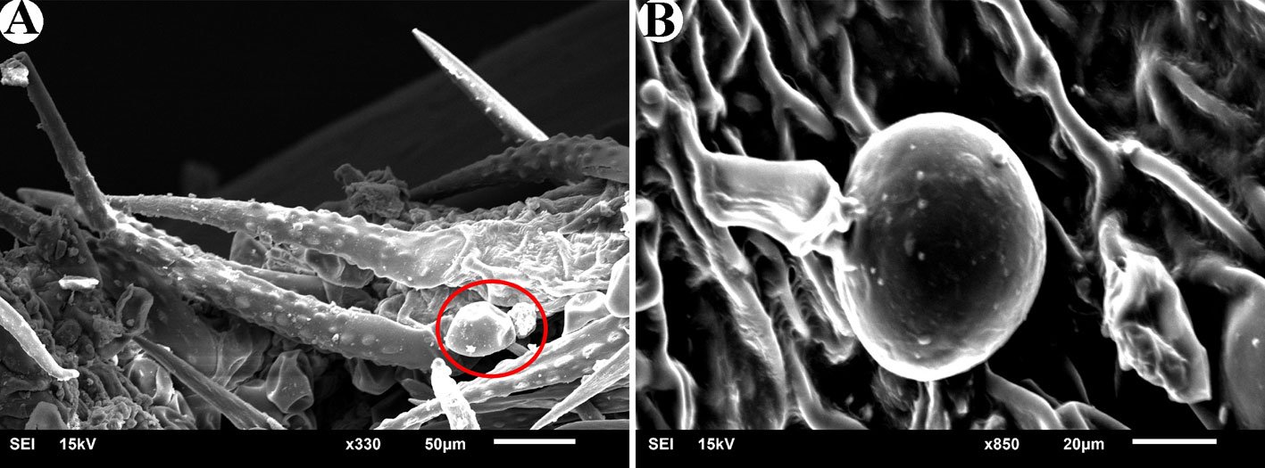
Figure 1. Glandular trichomes. A, Glandular trichomes (Icircled) next to non-glandular trichomes in Varronia bullata; B, glandular trichomes in Varronia guanacastensis.
Stellate trichomes are a type of branched trichome that have several arms arising from a common base (either stalked or sessile). This type of trichome was observed only in Cordia bicolor. The number of arms of these trichomes is between 10 and 17, and the length of each arm is between 50 and 100 μm. Figure 4 shows the studied specimen and the observed stellate trichome. The distribution and density of trichomes on the surface of the leaf can be seen with the naked eye most of the time. Figure 5 shows the leaves of the studied species where trichome density can be seen on their surface.
Microscopic examination of these 7 species revealed that the adaxial leaf surface generally has a lower density of trichomes compared to the abaxial surface, which has a higher density. On the adaxial surface of the leaf of Cordia africana, there are trichomes in the form of small protrusions that are sparse, while on the abaxial surface, the trichomes have a different shape and are densely placed inside the depressions, while long trichomes are rarely seen. In Cordia alliodora, C. bicolor, C. decandra, and C. myxa the type of trichome is similar on both surfaces, with the difference that they are scattered on the adaxial side and dense on the abaxial side. In the case of the 2 Varronia species, the trichomes are scattered on the adaxial surface of V. bullata and dense on the abaxial surface, but in V. guanacastensis, the trichomes are dense on both leaf surfaces, with the difference being that the type of trichome is different between the surfaces. Figure 6 shows the difference between trichome distribution on adaxial and abaxial leaf surfaces in all studied species.
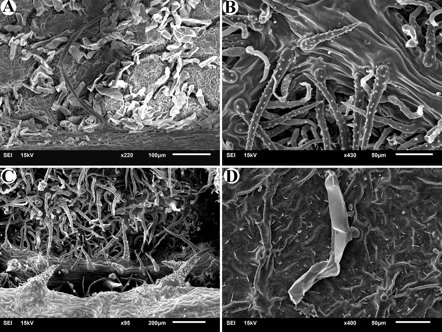
Figure 2. Non-glandular trichomes in studied species of Cordia. A, Abaxial surface in Cordia africana; B, abaxial surface in Cordia alliodora; C, abaxial surface in Cordia decandra; D, abaxial surface in Cordia myxa.
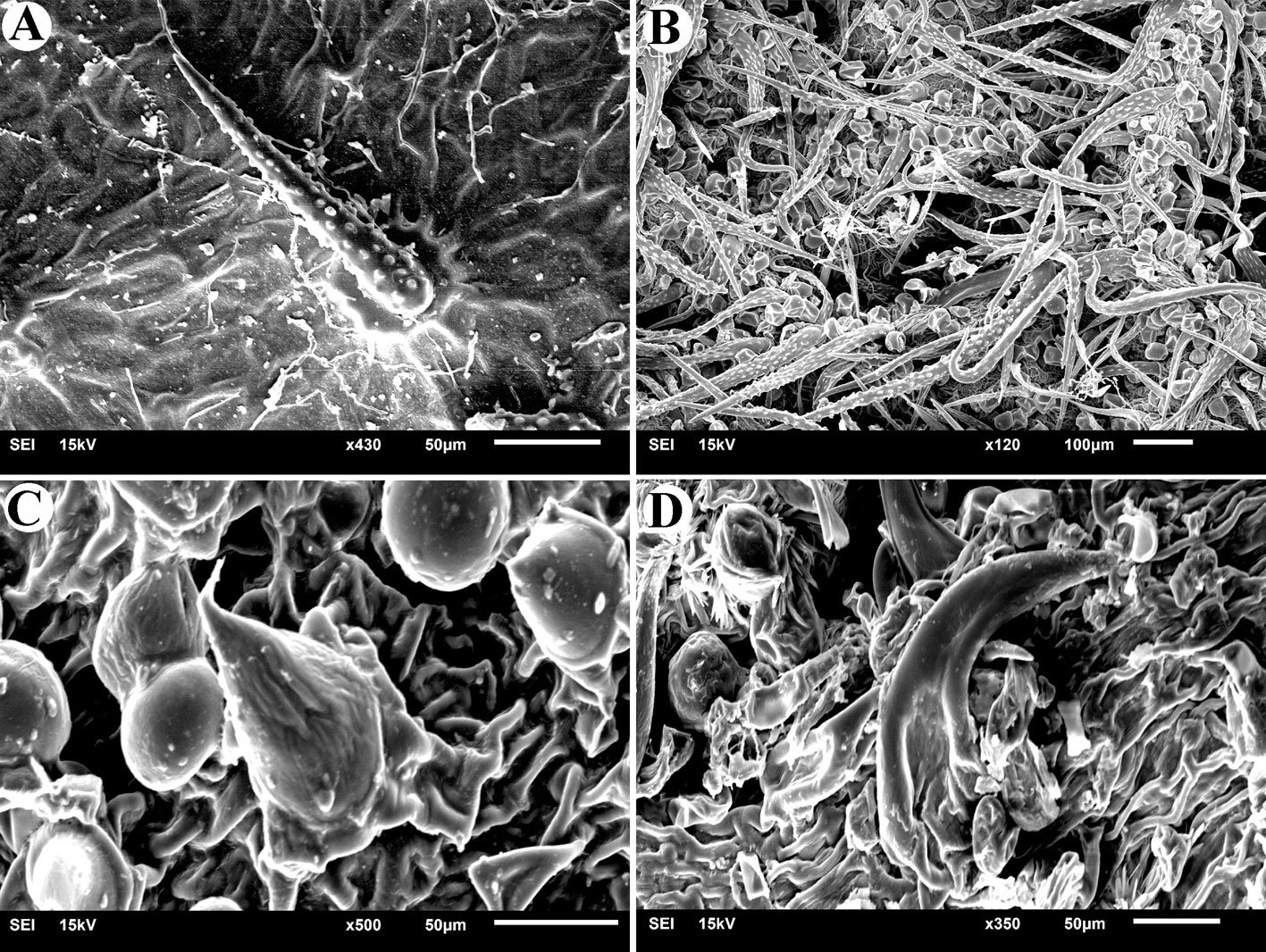
Figure 3. Non-glandular trichomes in studied species of Varronia. A, Adaxial surface in Varronia bullata; B, abaxial surface in Varronia bullata; C, adaxial surface in Varronia guanacastensis; D, abaxial surface in Varronia guanacastensis.
Discussion
Our study on leaf trichomes within Cordiaceae highlights significant morphological diversity, underscoring the diagnostic value of trichomes in taxonomy. Trichomes were categorized as either glandular (exclusively in Varronia species) or non-glandular (present in both genera), establishing clear taxonomic distinctions between the 2 genera. The restriction of glandular trichomes to Varronia supports the value of trichomes as reliable taxonomic markers, reinforcing molecular evidence that separates Varronia from Cordia. Despite the limited number of species examined, these findings offer a foundation for further studies across Cordiaceae. A notable finding was the discovery of stellate trichomes in Cordia bicolor, a first report for this species and probably rare within Boraginales. Stellate trichomes, characterized by multiple arms emerging from a common base, were observed solely in Cordia bicolor after an examination of over 100 Boraginales species (details in preparation). Figure 5 illustrates this unique stellate trichome, underscoring its taxonomic significance and its potential adaptive function.
Previous studies align with our findings on trichome diversity. Silva et al. (2023) examined leaf anatomy in 10 Varronia species from Brazil, identifying secretory and non-secretory trichomes as key taxonomic indicators. Similarly, Tölke et al. (2013) demonstrated variation in glandular and non-glandular trichomes among V. globosa Jacq. and V. leucocephala (Moric.) J.S. Mill., with unique glandular types and micropapillae-covered trichomes distinguishing each species. Demétrio et al. (2020) reported distinctive non-glandular trichomes and a single glandular type in V. polycephala Lam., a medicinal species, which also contained cystoliths and crystal sand idioblasts. These variations highlight trichomes as valuable taxonomic features and adaptive characters. While this study suggests a difference between Varronia and Cordia, the limited scope relative to the genera’s size precludes definitive conclusions. Further sampling of more species is needed to confirm this distinction in leaf trichomes.
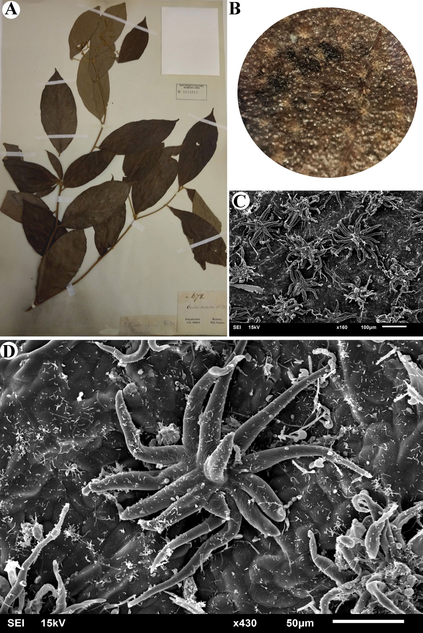
Figure 4. Stellate trichome in Cordia bicolor. A, studied specimen (W0010617); B, leaf surface visible with a normal magnification (X4); C, stellate trichomes are densely distributed on the leaf surface; D, stellate trichome with more than 10 arms.
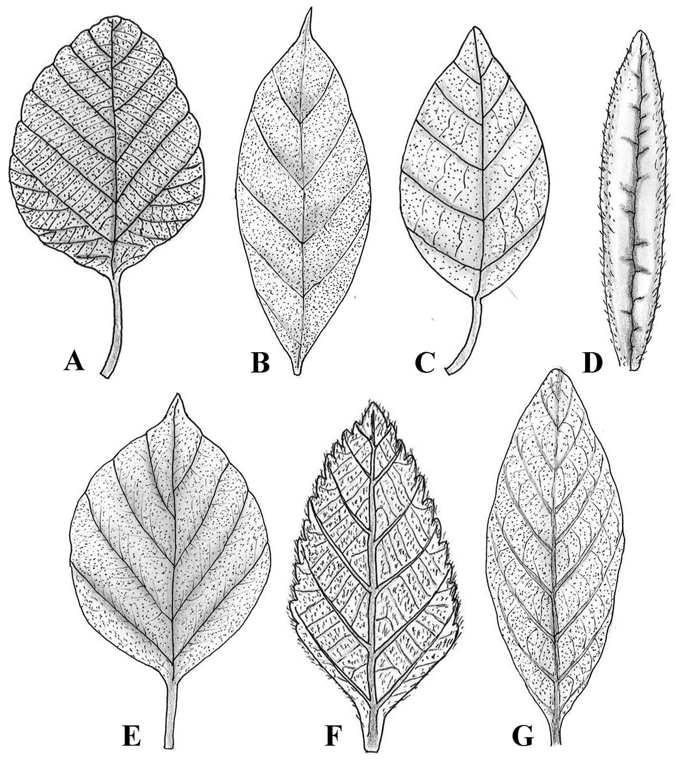
Figure 5. The distribution of trichomes on the adaxial leaf surface of the studied species of Cordiaceae. A, Cordia africana; B, Cordia alliodora; C, Cordia bicolor; D, Cordia decandra; E, Cordia myxa;F, Varronia bullata; G, Varronia guanacastensis.
Moreover, the distribution of trichomes, denser on the abaxial leaf surfaces, suggests adaptations to environmental pressures and provides additional taxonomic insight. Consistent trichome types on particular leaf surfaces across species indicate conserved characters, useful for classification within the family. This diversity, particularly in non-glandular trichomes that vary in shape, size, and density, emphasizes the evolutionary lability of trichomes and their dual roles in adaptation and taxonomy.
Our use of SEM enabled detailed trichome analysis, offering precise structural insights and enhancing taxonomic resolution. Nazari and Ghahremaninejad (2024, 2025) also found that trichome examination can verify generic separations within Boraginales, as demonstrated in their study on Heliotropiaceae. Collectively, these findings underscore the morphological and taxonomic significance of trichomes, establishing them as key indicators in botanical classification.
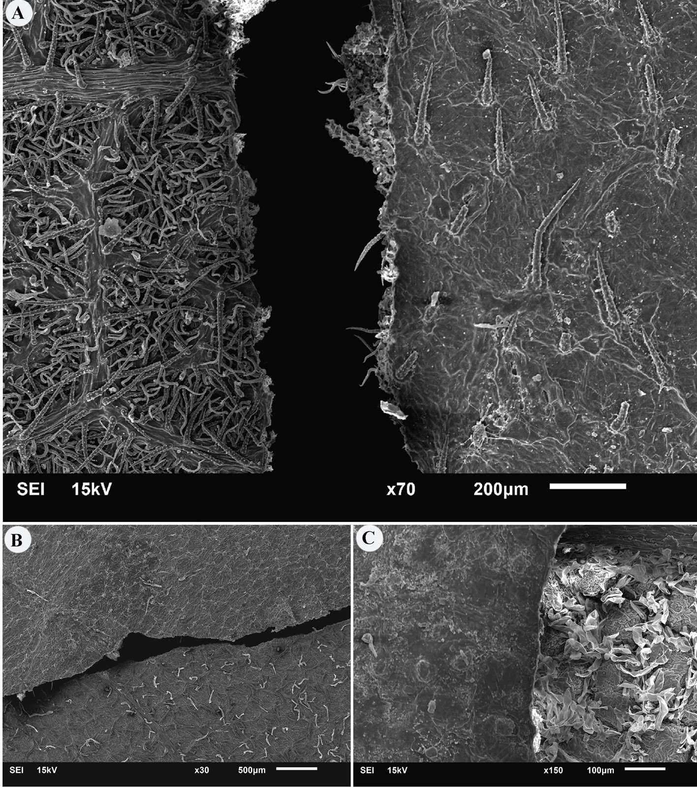
Figure 6. Differences in trichome distribution on adaxial and abaxial surfaces of some Cordia species. A, Cordia alliodora; B, Cordia myxa; C, Cordia africana.
Acknowledgments
We sincerely thank all the invaluable contributors to this work. Special thanks to Heimo Rainer, head of the Botany Department at the Natural History Museum of Vienna, for his extensive support. Additionally, we appreciate Astrid Hille, Andreas Berger, Tanja Schuster, and Johannes Walter from the same department for their assistance. We are also grateful to Wenke Wegner, a SEM specialist, for supervising the microscopic imaging of the fragments. Our thanks extend to W herbarium and B herbarium for sharing their extensive botanical resources.
References
Amer, W. M., Hamdy, R. S., & Mahdy, R. A. (2016). Taxonomic revision of genus Cordia L. (Boraginaceae) in Egypt. Egypt Journal of Botany, 6th International Conference, Menoufia University, 375–408.
APG IV. (2016). An update of the Angiosperm Phylogeny Group classification for the orders and families of flowering plants: APG III. Botanical Journal of the Linnean Society, 181, 1–20. https://doi.org/10.1111/boj.12385
Beilstein, M. A., Al-Shehbaz, I. A., & Kellogg, E. A. (2006). Brassicaceae phylogeny and trichome evolution. American Journal of Botany, 93, 607–619. https://doi.org/10.3732/ajb.93.4.607
Demétrio, A. M., Lusa, M. G., Lima, D. F., & Rodrigues, C. (2020). Leaf anatomy of Varronia polycephala Lam. (Cordiaceae). Flora, 271, 151677. https://doi.org/10.1016/j.flora.2020.151677
Flowers of India. (2025). Scarlet Cordia (Cordia sebestena). Retrieved March 7, 2025, from https://www.flowersofindia.net/catalog/slides/Scarlet%20Cordia.html
Ghahremaninejad, F. (2004). Value of trichome characteristics for separating of bifurcating Astragalus (Fabaceae) on sectional level. Turkish Journal of Botany, 28, 241–245.
Ghahremaninejad, F., Khalili, Z., Maassoum, A. A., Mirzaie-Nodoushan, H., & Riahi, M. (2012). Leaf epidermal features of Salix species (Salicaceae) and their significance. American Journal of Botany, 99, 769–777. https://doi.org/10.3732/ajb.1100019
Gonçales, R., Do Carmo, A. A. O., dos Santos, A. F., & de Souza, L. A. (2023). Floral indumentum of Miconia: In search of diagnostic characters for the tribe Miconieae. Revista Mexicana de Biodiversidad, 94, e945272. https://doi.org/10.22201/ib.20078706e.2023.94.5272
Johnston, I. M. (1951). Studies in the Boraginaceae XX. Representatives of three subfamilies in eastern Asia. Journal of the Arnold Arboretum, 32, 99–122. https://doi.org/10.5962/bhl.part.9730
Kong, M. J., & Hong, S. P. (2019). Leaf micromorphology of the Persicaria sect. Cephalophilon (Polygonaceae) and its systematic re-evaluation. Phytotaxa, 391, 167–184. https://doi.org/10.11646/phytotaxa.391.3.1
Luebert, F., Cecchi, L., Frohlich, M. W., Gottschling, M., Guilliams, C. M., Hasenstab-Lehman, K. E. et al. (2016). Familial classification of the Boraginales. Taxon, 65, 502–522. https://doi.org/10.12705/653.5
Matias, E. F. F., Alves, E. F., Silva, M. K. N., Carvalho, V. R. A., Coutinho, H. D. M., & da Costa, J. G. M. (2015). The genus Cordia: Botanists, ethno, chemical and pharmacological aspects. Revista Brasileira de Farmacognosia, 25, 542–552. https://doi.org/10.1016/j.bjp.2015.05.012
Miller, J. S., & Gottschling, M. (2007). Generic classification in the Cordiaceae (Boraginales): Resurrection of the genus Varronia R.Br. Taxon, 56, 163–169. https://doi.org/10.2307/25065747
Nazari, H., & Ghahremaninejad, F. (2024). A SEM study of leaf trichomes in Heliotropiaceae. Iranian Journal of Botany, 30, 173–183. https://doi.org/10.22092/ijb.2024.366196.1475
POWO. (2024). Plants of the World. Online. https://powo.science.kew.org/
Rodríguez, A., & Healey, P. L. (2000). Morphological diversity of trichomes in Loasaceae and its systematic significance. Annals of the Missouri Botanical Garden, 87, 71–86. https://doi.org/10.1093/aobpla/plab071
Selvi, F., & Bigazzi, M. (2001). Leaf surface and anatomy in Boraginaceae tribe Boragineae with respect to ecology and taxonomy. Flora, 196, 269–285. https://doi.org/10.1016/S0367-2530(17)30056-7
Silva, T. S., & de Melo, J. I. M. (2019). A new species and a new record of Varronia (Cordiaceae) from Brazil. Systematic Botany, 44, 692–696. https://doi.org/10.1600/036364419×15620113920752
Silva, T. S., Tölke, E. E. D., & de Melo, J. I. M. (2023). A contribution of leaf anatomy to the taxonomy of Varronia P. Browne (Cordiaceae, Boraginales). Flora, 304, 152299. https://doi.org/10.1016/j.flora.2023.152299
Steyn, H. M., & Van Wyk, A. E. (2021). Taxonomic significance of trichomes in the genus Acanthopsis Harv. (Acanthaceae, tribe Acantheae). Adansonia, 43, 163–176. https://doi.org/10.5252/adansonia2021v43a14
Taroda, N. (1984). Taxonomic studies on Brazilian species of Cordia L. (Boraginaceae) (Ph.D. Thesis). University of St. Andrews. St. Andrews, UK.
Thiers, B. M. (2025). Index Herbariorum: a global directory of public herbaria and associated staff (Continuously updated). New York Botanical Garden’s Virtual Herbarium. http://sweetgum.nybg.org/ih/
Tölke, E. E. D., de Melo, J. I. M., Carmello-Guerreiro, S. M., & Lacchia, A. P. S. (2013). Leaf anatomy with emphasis on separation of two species of Varronia P.Br. (Cordiaceae) of the Brazilian semi-arid region. Brazilian Journal of Botany, 36, 189–201. https://doi.org/10.1007/s40415-013-0022-5
Wagner, G. J. (1991). Secreting glandular trichomes: more than just hairs. Plant Physiology, 96, 675–679. https://doi.org/10.1104/pp.96.3.675

Notes on Cybistrinae from Mexico (Coleoptera: Dytiscidae), with the description of 2 new species of Trifurcitus
Roberto Arce-Pérez, Andrés Ramírez-Ponce *
Instituto de Ecología, A.C., Red de Biodiversidad y Sistemática, Carretera Antigua a Coatepec Núm. 351, El Haya, 91073 Xalapa, Veracruz, Mexico
*Corresponding author: andres.ramirez@inecol.mx (A. Ramírez-Ponce)
http://zoobank.org/urn:lsid:zoobank.org:pub:A0A5D659-2677-4CE4-BAA3-7162B5338BCF
Abstract
A bibliographic and museum review is carried out on the Cybistrinae species of Mexico, as well as comparative analysis with species from South America, concluding that Trifurcitus fallax (Aubé, 1838) has been wrongly cited for Mexico. Additionally, 2 new species are described as the first country-specific records, Trifurcitus mexicanus sp. nov. from the state of Chiapas, and T. maya sp. nov. from the state of Yucatán. Also, new state records are provided for Bifurcitus lherminieri (Guérin-Méneville, 1829) in Mexico. Future reviews of specimens under the names Bifurcitus, Cybister, Metaxydytes, and Trifurcitus are recommended as this could likely uncover more new species.
Keywords: Coleoptera; Dytiscidae; Cybistrinae; Trifurcitus; Bifurcitus; Mexico; New species
Notas sobre Cybistrinae de México (Coleoptera: Dytiscidae), con la descripción de 2 especies nuevas de Trifurcitus
Resumen
Se realiza una revisión bibliográfica y museística de las especies de Cybistrinae de México, así como un análisis comparativo con especies de Sudamérica, concluyendo que Trifurcitus fallax (Aubé, 1838) ha sido citada erróneamente para México. Adicionalmente, se describen 2 especies nuevas como los primeros registros específicos para el país, Trifurcitus mexicanus sp. nov. del estado de Chiapas, y T. maya sp. nov. del estado de Yucatán. También se proporcionan registros nuevos estatales para Bifurcitus lherminieri (Guérin-Méneville, 1829) para México. Se recomiendan revisiones futuras de especímenes bajo los nombres Bifurcitus, Cybister, Metaxydytes y Trifurcitus, ya que éstos, probablemente, podrían incluir más especies nuevas.
Palabras clave: Coleoptera; Dytiscidae; Cybistrinae; Trifurcitus; Bifurcitus; México; Especies nuevas
Introduction
Until recently, the subfamily Cybistrinae Sharp, 1880 included 1 tribe, 7 genera, 8 subgenera and 129 species with 10 subspecies worldwide (Nilsson & Hájek, 2023), including 2 genera from the New World: Megadytes Sharp, 1880, with 21 species in 4 subgenera, and Cybister Curtis, 1827, with 6 species in 2 subgenera and additional species without subgeneric assignment (Arce-Pérez et al., 2021; Nilsson & Hájek, 2023; Trémouilles, 1984, 1989a, b; Trémouilles & Bachmann, 1980). A phylogenetic study (Miller et al., 2024) based on morphological characters, focused on reclassifying the genera of Cybistrinae, updated the information including 1 tribe, 12 genera, 4 subgenera and 130 species with 10 subspecies (Miller et al., 2024). In this work, for the New World 7 genera were included: Bifurcitus Brinck, 1945 (3 species), Cybister Curtis, 1827 (5 species in 2 subgenera), Megadytes Sharp, 1882 (2 species), Metaxydytes Miller et al., 2024 (9 species), Nilssondytes Miller et al., 2024 (1 species), Paramegadytes Trémouilles & Bachmann, 1980 (2 species), and Trifurcitus Brinck, 1945 (6 species).
Of the 7 genera cited for the New World, 4 are reported for Mexico, Bifurcitus (2 species), Cybister (3 species), Metaxydytes (2 species), and Trifurcitus (1 species) (Arce-Pérez et al., 2021; Miller et al., 2024; Nilsson & Hájek, 2023). The only species of Trifurcitus cited for Mexico by Sharp (1882a, b), T. fallax (Aubé, 1838), was described from French Guyana. Dejean (1836: 60) lists it as Trochalus fallax from Cayenne. This name was made available by Aubé (1838: 54) as Cybister fallax. Sharp (1882a: 710 and 1882b: 47) placed the species in his new genus Megadytes, and Brinck (1945: 8) in his new subgenus Trifurcitus of Megadytes. Currently the species is classified in the genus Trifurcitus (Miller et al., 2024). Sharp (1882a, b) studied a female from the Edwin Brown collection reported it from Mexico without a precise locality. Wilke (1920: 247) cited 1 specimen from the British Museum from “Mexico” and another from “Orizaba-Mexico” (State of Veracruz). Zimmermann (1920: 256) listed Sharp’s specimen but cited it incorrectly from Central America. Trémouilles and Bachmann (1980: 125) and Trémouilles (1989b: 161) cited the species for Argentina, Bolivia and Brazil. Libonatti et al. (2013: 164) were the last to provide a new record of the species (Chaco province, Argentina). The larval stages of T. fallax were described by Ferreira (1995: 315) and Michat (2010: 381). Arce-Pérez et al. (2021: 331) provided a key for all the New World Cybistrinae species found north of Belize and Guatemala, including T. fallax.
For Mexico, there are no records later than those of Sharp (1882a, b) and Wilke (1920). Now, 104 years after, while reviewing Cybistrinae material from different Mexican collections, some specimens were found identified as T. fallax. However, while undertaking a comparative analysis with specimens from Argentina, Bolivia, Brazil and México housed in different museums, Sharp’s opinions stand out: “I have seen only two individuals of this species, one of them, from Dejean’s collection, was there labelled “Trochalus fallax mihi, h. in Cayenne, D. Lacordaire”: the other was in Edwin Brown’s collection and labelled in his handwriting “Cybister flavocinctus, Chev., Mexico.” The determination being wrong it is probable that the locality also of this latter specimen may be erroneous. Cayenne.; 1 Mexico. 1107” (Sharp, 1882a). “This little-known species is represented in Salle’s collection by a single female labelled “Trogus flavocinctus”, this determination, however, was erroneous and the specimen, a very fine one, agrees with the 2 other female, these being all that we know of the species” (Sharp, 1882b).
Based on the above, we consider that T. fallax is only distributed in South America (Argentina, Bolivia, Brazil and French Guiana), and therefore, the Mexican specimens correspond to another species, whose description is the objective of the present work.
Materials and methods
Type material and other specimens of Trifurcitus fallax (Aubé, 1838) were requested in different national and foreign museums. Four male specimens from Mexico were examined (CNIN), plus another dissected one and housed at BMNH by photographic comparison. The 4 Mexican specimens were hydrated in a humid chamber for 2 days, their genitals were removed and cleaned in hot water. The median lobe and parameres were disarticulated and mounted with the specimens. Two male specimens dissected from Argentina (MACN) determined by Trémouilles and Bachmann (1980) were reviewed in photographs as well as undissected specimens from Brazil and Bolivia deposited in collections in Germany (ZSM) (MZSP) and Brazil, that were used for comparison.
The Mexican specimens were studied with a LEICA MZ8 stereomicroscope and photographed with a Zeiss Stemi SV6 stereomicroscope, stacking several photographs into a final image. The final plates were edited in Photoshop CS6. The reviewed specimens come from the following collections —specimens reviewed directly: Colección Nacional de Insectos (CNIN), Instituto de Biología, Universidad Nacional Autónoma de México, Mexico City, Mexico (S. Zaragoza); Colección de Insectos del INECOL (IEXA), Instituto de Ecología A.C., Xalapa, Veracruz, Mexico (R. Arce-Pérez). Specimens reviewed by photographs: Museo Argentino de Ciencias Naturales (MACN), Buenos Aires, Argentina (P. Mulieri); Muséum National d’Histoire Naturelle (MNHN), Paris, France (website); Museu de Zoologia da Universidade de São Paulo (MZSP), Sao Paulo, Brazil (S. Casari); The Natural History Museum (BMNH), London, UK (M. Geiser); and Zoologische Staatssammlung München (ZSM), Germany (M. Balke).
Results
Historiographical analysis allowed us to trace the depository of type material from Cayenne (French Guiana). Unfortunately, the specimens are lost, as it is the material from Bolivia (MNHN) identified by Trémouilles and Bachmann (1980). Only 1 female syntype was compared from the website of MNHN, and dissected males were also used from Mexico (BMNH) and Argentina (MACN), and specimens from Brazil (MZSP) and Bolivia (ZSP) (not dissected) for comparison via photographs.
When trying to compare the diagnostic characters presented in the original description made by Aubé (1838), the diagnosis of Sharp (1882a, b), and the diagnosis of Trémouilles and Bachmann (1980), the identity of Mexican specimens of T. fallax could not be confirmed. This was also observed in studies that addressed with the larva of T. fallax; when describing the third stage (1 from Brazil and another from Argentina), they appear as different species (Fig. 1a, b) (Ferreira, 1995; Michat, 2010), probably because the associated adults were different species, but were identified with the key of Trémouilles and Bachmann (1980) arriving to M. (T.) fallax.
The larva illustrated by Michat (2010) is now recognized as T. fallax (Miller et al., 2024). Also by making the determination by photographic comparison with specimens determined by specialists (determination labels of Guignot [1955, 1958], Bachmann [1979] and Trémouilles [1985]) deposited in several museums (MZSP, ZSM, BMNH) (Fig. 2a, f), among them a syntype female (MNHN), and by morphological comparison with the specimens 7715 and 7725 of the Museo Argentino de Ciencias Naturales, where it was observed that they are generally similar to the specimens from Mexico (length, shape, color, punctures) but differ in the diameter of the dorsal puncture and of ventrites III to V, being slightly thicker and denser in the South American specimens (Fig. 3a, h).
The specimens from Argentina, Bolivia and Brazil have transverse rows on ventrites III to V, plus a slight central accumulation of points in ventrite III (Fig. 3b, d, f, h); while the Mexican specimens present finer punctuations, with a transverse row in ventrites IV and V, and few central punctuations in ventrite III (Figs. 5b, 8b). The basal impression of the prosternal process in the specimens from Argentina (MACN) is variable, being present in specimen 7715 and completely absent in specimen 7725 (Fig. 3b), while in the specimens from Mexico it is present in Trifurcitus mexicanus nov. sp. (Fig. 5b, d), and absent in T. maya nov. sp. (Fig. 8b), also visible in the Bolivian specimen (Fig. 3d) and not observable in the Brazilian specimen (Fig. 3h).
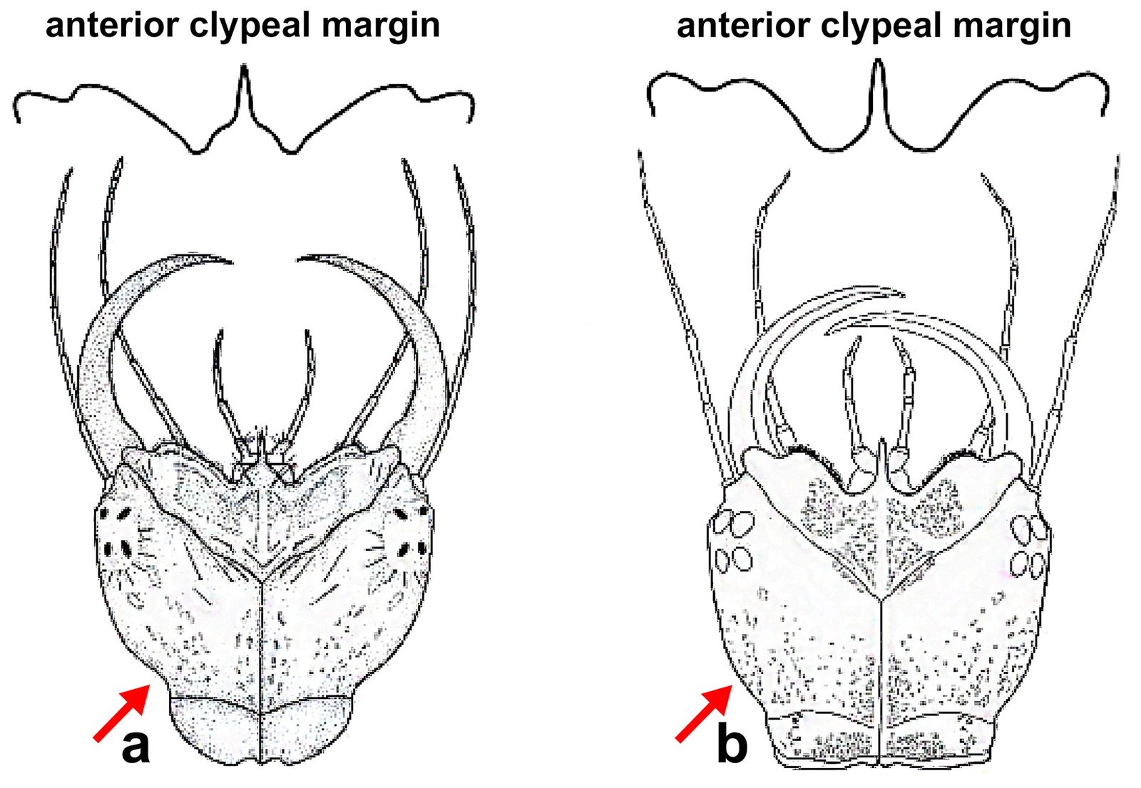
Figure 1. Front view of the head of larva III of Trifurcitus fallax. a) Sensu Ferreira (1995); b) sensu Michat (2010).
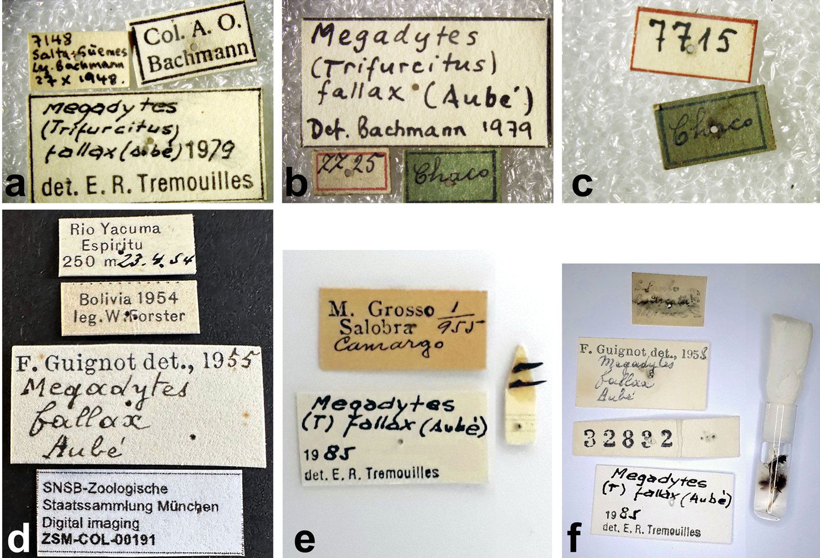
Figure 2. Identification labels of Megadytes fallax (Aubé, 1838) deposited in different museums: a-c, Museo Argentino de Ciencias Naturales, Buenos Aires, Argentina; d, Museu de Zoologia da Universidade de São Paulo, Sao Paulo, Brazil; e, f, Zoologische Staatssammlung München, Germany.
Furthermore, the shape of the median lobe of the male genital in the Argentinean specimens and in the illustrations by Trémouilles and Bachmann (1980) is narrower and sharper at the apex (Fig. 4a, b, d, e) while in Mexican specimens it is slightly to moderately wider (Figs. 6a-f; 8c-e), In addition, the distance between the apex of the ventral sclerite and the apex of the median lobe appears to be smaller in South American specimens (these measurements may vary due to dehydration) (Figs. 4b, e, 6a, e, f, 8d, e).
The distribution of the species of Trifurcitus is Neotropical (Argentina, Bolivia, Brazil, French Guiana, and Panama), with T. fallax being recorded from Argentina, Bolivia, Brazil, and French Guiana (Nilsson & Hájek, 2023; Trémouilles & Bachmann, 1980), making its presence in Mexico unlikely. Historical analysis, morphological comparison and communication with specialists of the group allow us to support what was mentioned by Sharp (1882a, b), that T. fallax does not reach Mexico, and to report 2 new species of this genus for Mexico, T. mexicanus nov. sp. Arce-Pérez & Ramírez-Ponce for Chiapas, and T. maya nov. sp. Arce-Pérez & Ramírez-Ponce for Yucatán, representing the first records of the genus Trifurcitus Brinck for Mexico.
Descriptions
Trifurcitus mexicanus Arce-Pérez & Ramírez-Ponce, sp. nov.
(Figs. 5a-d, 6a-g)
http://zoobank.org/urn:lsid:zoobank.org:act:C402DD76-
7886-4E02-A8CD-20961D87851F
Differential diagnosis. The new Mexican species can be differentiated from the South American ones by the diameter of the dorsal punctuation, and of ventrites III to V (Fig. 5a, b), being slightly thicker and denser in the South American specimens (Fig. 3a-h). In addition, the shape of the middle lobe of the male genital in South American specimens is narrower and sharper at the apex (Fig. 4a, b, d, e), while in Mexicans it is slightly to moderately wide (Fig. 6a, b, d, e).
Description. Holotype (male, IEXA).Habitus and general surface structure: dorsal (Fig. 5a); body oval, maximum width behind of the half of the elytral length. Length 29 mm, maximum width 18 mm. Dorsal coloration dark olive green shiny, with wide reddish-yellow stripe along the lateral margins of the pronotum and elytra, near the elytral apex the olive-green coloration is interspersed with yellow punctuation of the lateral stripe; clypeus anteriorly and labrum reddish-yellow. Ventral coloration (Fig. 5b) black, with reddish-yellow palps and antennae, yellowish-reddish front and middle legs, black hind legs. Sculpture on dorsum and venter largely smooth; with punctuations of variable diameter and faint wrinkles and striae; the setation is minute, slender and sparse, present in punctuations and often almost imperceptible. Median lobe wider in its basal half (0.55 mm), narrowing apically, apex slightly rounded (Fig. 6a, e). Dorsal surface (Fig. 5a, c), head: clypeus with almost straight anterior margin, labrum with slightly sinuous anterior margin, with small central concavity. Clypeal line incomplete, widely interrupted medially. Two small, punctuate grooves transverse, immediately posterior to anterior margin. Strongly punctuate oval longitudinal depression on each side posterior to incomplete clypeal line. Short row of small punctures along the posterior half of inner margin of eyes (Fig. 5c). Antennae filiform. Both palps are slender, but slightly thicker than the reddish-yellow antennae. Setae very short, sparse in the grooves of the clypeus; thicker and denser in the concavity of the labrum; slightly longer in the longitudinal depression posterior to the interrupted clypeal line; very short and sparse on the inner margins of the eyes. Surface of the vertex with slight longitudinal wrinkles. Pronotum: anterior margin with short rows of small punctures interrupted medially; line of punctures slightly thicker, extending laterally reaching inner margin of reddish-yellow stripe; inner margin of stripe with scattered row of thicker punctures extending from base to apex. Surface with faint longitudinal striations and wrinkles, mainly in the posterior region, and a slight accumulation of punctures on each side of the disc. Lateral margin without edge, with complete yellowish-reddish band, which exceeds the yellowish-reddish border of the hypomeron. Short setae on the punctuation of the anterior edge, lateral margins and on the yellowish-reddish band. Elytra:3 longitudinal lines defined by broad and widely separated punctuations; first line with slightly elongated punctuations reaching near the apex; second and third lines with circular punctuations; third line at inner edge of reddish-yellow stripe. Elytral margins with a thick, complete border and minute, irregular punctuation; dark olive-green margins in anterior half. Reddish-yellow band along the margin of the elytra, not reaching the margin or the epipleura, more or less of equal width throughout its length, defined as a network of irregular polygonal pigments, which mixes with the dorsal olive-green colour as scattered dots. Very sparse setiferous punctuation on the yellow stripe and lateral edge; very short setae. Ventral surface (Fig. 5b, d), head:shiny black; mouthparts dark reddish; antennae and palps reddish-yellow. Prothorax:shiny black; hypomeron yellowish-reddish. Prosternal process subrectangular in anterior half, flat surface, anterior edge not notched, continuing into an oval depression with rounded apex; posterior half widened and lanceolate, pointed, reaching the deeply triangular anteromedial process of the metaventrite; lanceolate region with a lateral rim, and the apex acute with transverse striations (Fig. 5d), length 4.1 mm long by 1.3 mm wide. Pterotorax: epipleuron reddish-yellow, broad, with slight mesial narrowing. Suture between metaventrite and metacoxal plates weakly marked. Metaventrite with conspicuous curved row punctuationss in anteromedial region. Metacoxal lines strongly divergent anteriorly, not reaching anterior margin of metaventrite; with row of broad punctures extending beyond metacoxal lines to suture of metaventrite. Posterior margin of metacoxal processes with deep central triangular incision; lobes of processes broadly rounded. Abdomen: colour: shiny black, with a semicircular reddish-yellow spot on lateral margin of ventrites III to V; with a slight lateral depression in ventrites II to VI, deeper and expanded in ventrites V and VI; suture between ventrites I and II clearly marked; ventrite III with few, tiny punctures and wrinkles on middle and parallel wrinkles on distal margin; ventrites IV and V with transverse line of small punctures and superficial wrinkles (evident in ventrite V); ventrite VI with uniformly rounded apex, with a slight transverse depression, with the lateral depression deeper and more extended, with few, tiny scattered punctures. Setiferous puncture, with very short yellowish setae. Legs:front and middle legs reddish-yellow, hind legs black, with a light reddish trochanter in its apical half. Protarsomere I-III enlarged, oval-shaped; 1.3 mm long by 1.9 mm wide; protarsomere I with numerous minute sucking setae at base and a row of large sucking setae at apex, protarsomere II with only 1 row of large sucking setae, protarsomere III with 2 rows of large sucking setae, protarsomere V with a pair of long, black, curved, sharp claws; anterior claw longer and thicker. Mesotarsomeres dark; mesotarsomeres I-IV with a series of setae near apical margin (posteroventrally); mesotarsomeres I-II with abundant ventral rows of long pale-yellow setae; claws sharp and curved, the anterior one longer and thicker; both longer and thicker than the protarsal claws. Metafemur with rounded dorso-distal angle, weakly acute (almost straight), not pointed. Metatibia with 2 apical spurs, the outer one noticeably thinner than the inner one and with trifid apex. Last metatarsomere with 2 straight and sharp claws of equal length, the outer one slightly wider. Male genitalia (Fig. 6a-g). Median lobe wider in its basal half (0.55 mm), narrowing apically, apex slightly rounded (Fig. 6a, e). Median lobe in lateral view, length 4 mm (Fig. 6d, f); ventral, with maximum width 0.55 mm (Fig. 6e); ventrolateral (oblique view) 4 mm (Fig. 6f), and median sclerite 3 mm (Fig. 6e). Distance between the apex of the median sclerite and the apex of the median lobe 1 mm (Fig. 6e); Left paramere 4 mm, with row of external ridges, in oblique view, the ridges that reach the ventral margin in the apical 3/3 simulate small teeth (Fig. 6g).
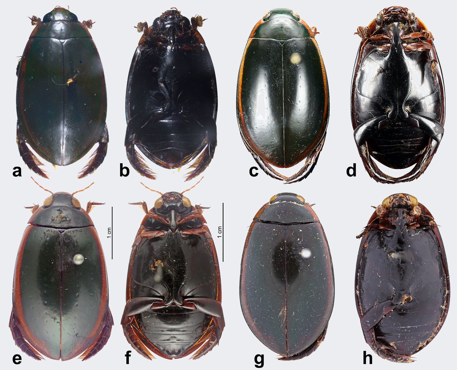
Figure 3. Dorsal and ventral view of Trifurcitus fallax housed in different museums: a, b, Museo Argentino de Ciencias Naturales, Buenos Aires, Argentina; c, d, Zoologische Staatssammlung München, Germany; e, f, Muséum National d’Histoire Naturelle Paris, France; g, h, Museu de Zoologia da Universidade de São Paulo, Sao Paulo, Brazil.
Variation. A male specimen like the holotype (without genitalia) from Chiapas, Municipality of Cintapala (16°37’ N, 93°46’ W), 28.III.1985, Col. M.L. Lozano. “Small (length 27 mm, width 16.5 mm), dorsally, slightly brownish coloration; surface on the pronotum with more wrinkles on the disk; more evident stippling and wrinkles on ventricles III to V.”
Females. Not present in the material studied. According to Trémouilles and Bachmann (1980), females present sexual sculpture formed by curved, anastomosing lines, or without sexual sculpture, and according to Aubé (1838), the females differ only by the simplicity of the front legs.
Taxonomic summary
Type locality:Mexico, Chiapas, Municipality of Concordia, km 17 carretera Jaltenango-Revolución Mexicana, 15°58’ N, 92°48’ W, elevation 575 m asl.
Type material:holotype: ♂, México: Chiapas/Municipio de Concordia, 15°58’ N, 92°48’ W/18-V-2012, Col. D. Reynoso-Velasco [typed, white label], “holotipo/Trifurcitus mexicanus nov. sp./Arce-Pérez & Ramírez-Ponce 2024” [typed, red label] (IEXA).
Habitat: Megadytes species have been reported to be associated with open, sunny environments in permanent and temporary lentic waters with dense vegetation; however, detailed habitat preferences are unknown for most species (Miller & Bergsten, 2016), except for Bifurcitus iherminieri (Hendrich et al., 2019). The specimen from Chiapas (Municipality of Concordia), was collected in a sunny and exposed area, on the banks of a permanent, slow-flowing stream, with an average depth of 80 cm, among grasses that grow on the riverbank (Fig. 7a, b) (Daniel Reynoso Velasco, personal communication).
Distribution: this species is known from Mexico, Chiapas, but being a species of a Neotropical genus, it is likely that it is also distributed in Oaxaca and Guatemala on the Pacific coast.
Etymology: because it is the first corroborate record of the genus Trifurcitus Brinck for the country, this species is named mexicanus.
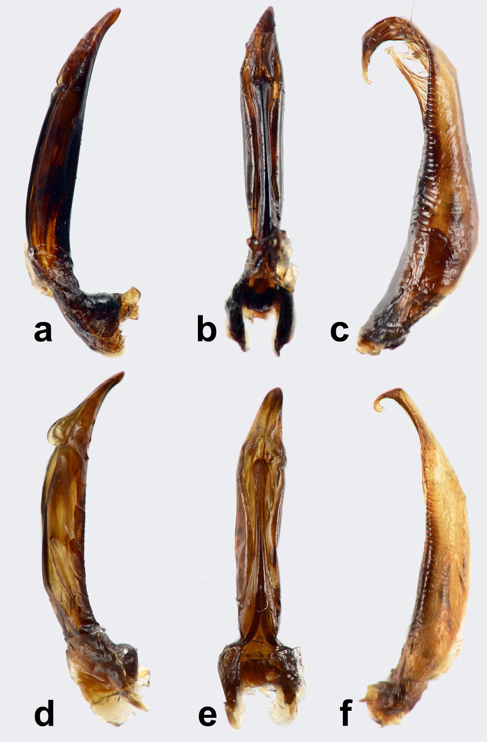
Figure 4. Lateral and ventral view of the middle lobe and left paramere of Megadytes (T.) fallax housed at Museo Argentino de Ciencias Naturales, Buenos Aires, Argentina: a-c, specimen number 7715; d-f, specimen number 7725.
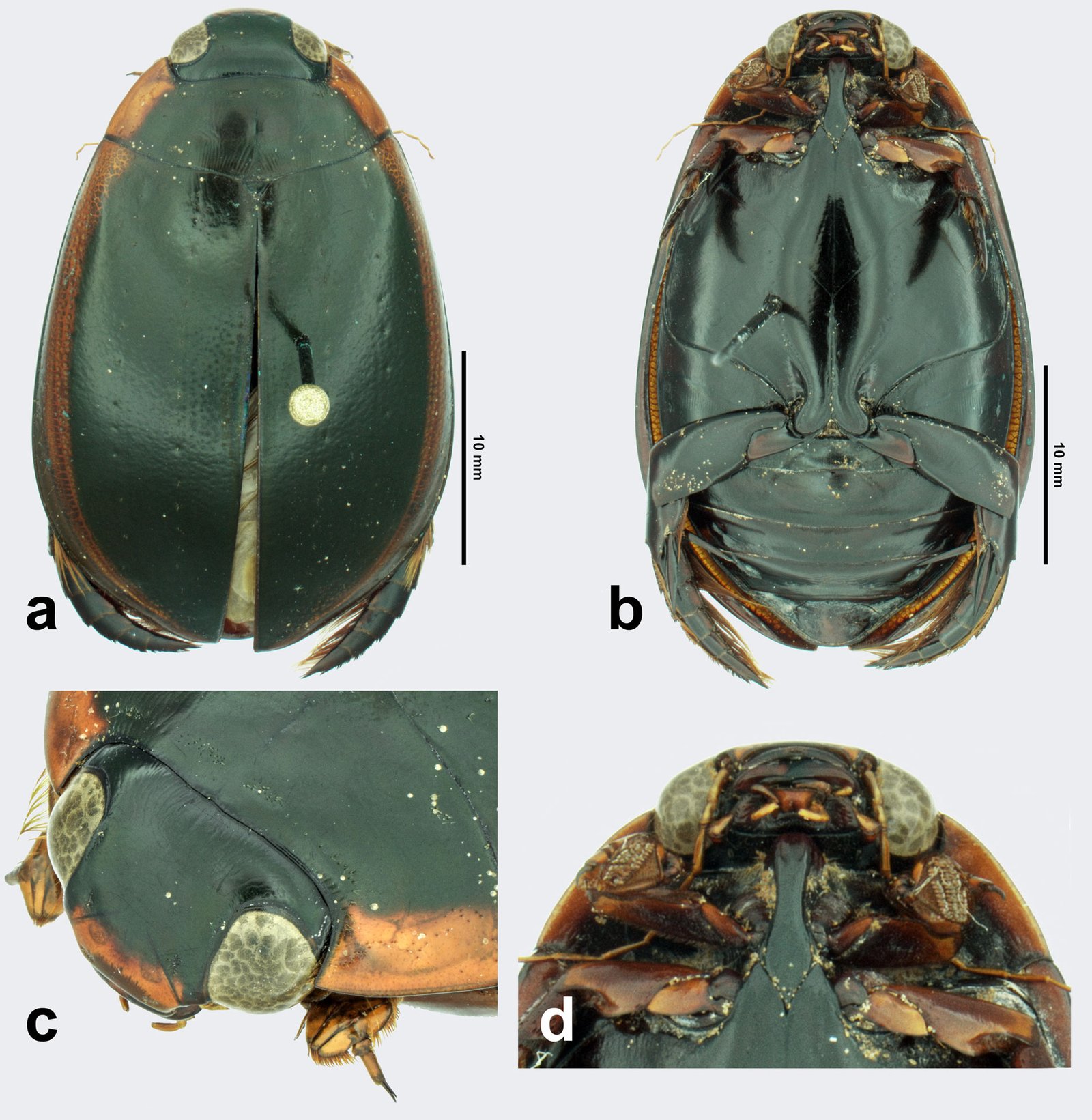
Figure 5. Habitus of Trifurcitus mexicanus sp. nov. a, dorsal view; b, ventral view; c, oblique view of the head; d, view of the prosternal process.
Remarks
Trifurcitus mexicanus sp. nov. can be differentiated from Trifurcitus maya sp. nov. by the following characters (Trifurcitus maya nov. sp. [in brackets]). Trifurcitus mexicanus presents an oval depression with rounded apex in the anterior half of the prosternal process (Fig. 5d) [without depression (Fig. 8b)]; ventrites IV and V with a transverse line of small punctures and superficial wrinkles (Fig. 5b) [ventrite IV without apparent punctuation or wrinkles (Fig. 8b)]; Male genitalia in ventral view with broad median lobe in its basal half (0.55 mm), slightly narrowing apically and with rounded apex (Figs. 6a, e) [median lobe slender in basal half (0.53 mm), narrowing apically and with apex acute (Fig. 8d)].
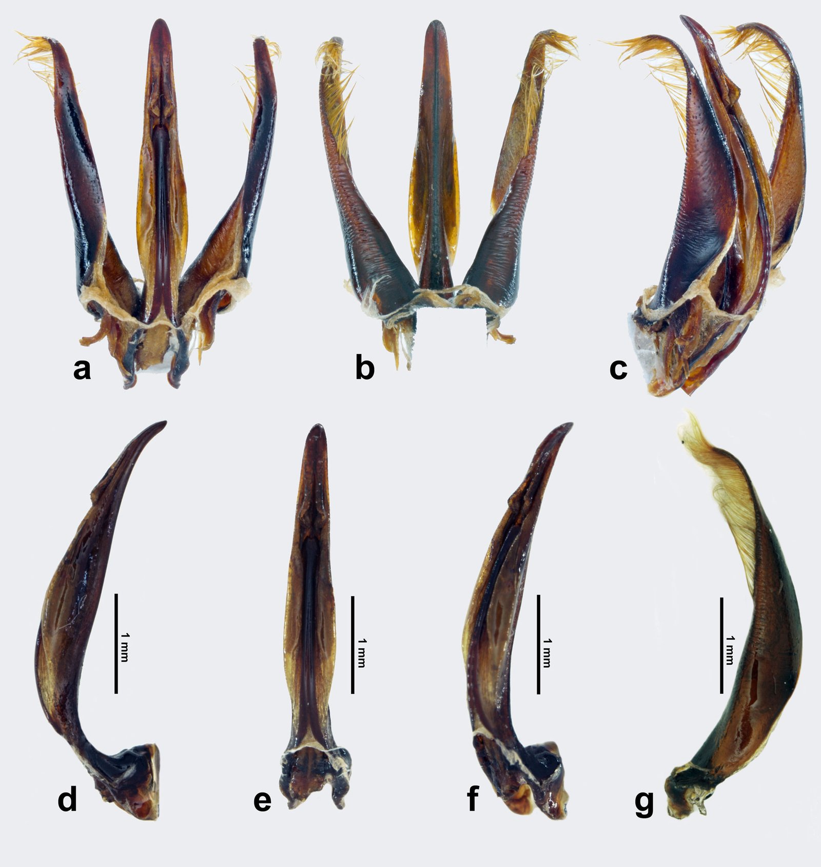
Figure 6. Male genitalia of Trifurcitus mexicanus nov. sp. (holotype): a-c, full ventral, dorsal and oblique view of parameres and median lobe; d-f, lateral, ventral and oblique view of the middle lobe; g, lateral view of left paramere.
Trifurcitus maya Arce-Pérez & Ramírez-Ponce, sp. nov.
(Fig. 8a-f)
http://zoobank.org/urn:lsid:zoobank.org:act:DEA31260-8EC4-47D7-AE64-9EA426F102BF
Differential diagnosis. In Trifurcitus mexicanus Arce-Pérez & Ramírez-Ponce.
Description. Habitus and general surface structure: dorsal (Fig. 8a): bodyoval, maximum width behind the half of the elytral length. Length 29 mm, 17 mm wide. Coloration bright dark olive green, with a broad reddish-yellowish stripe along the lateral margins of the pronotum and elytra, near the elytral apex interspersed with the yellow punctuation of the lateral band; clypeus anteriorly and labrum reddish-yellowish. Ventral (Fig. 8b): black coloration with reddish-yellow palps and antennae, dark reddish front and middle legs, black hind legs. Sculpture dorsal and ventral largely smooth, with punctuations of variable diameter and faint wrinkles and striae; the setation is minute, slender and sparse, present only at punctuations and often almost imperceptible. in ventral view, with median lobe slender in its basal half (0.53 mm), narrowing apically, with apex slightly acute (Fig. 8c-e). Dorsal surface (Fig. 8a), head: clypeus with almost straight anterior margin, labrum with slightly sinuous anterior margin, with small central concavity. Clypeal line incomplete, widely interrupted medially. Two small, punctuations grooves transverse, posterior to anterior margin. A punctuate oval depression on each side, posterior to incomplete clypeal line. A short line of small punctures along posterior half of inner margin of eyes. Antennae filiform. Both palps thin, like the antennae, reddish-yellow. Setae very short, sparse in the grooves of the clypeus; denser and thicker in the concavity of the labrum; slightly longer in the oval depression posterior to the interrupted clypeal line; very short and sparse on the inner margins of the eyes. Front surface with slight longitudinal wrinkles on the posterior half. Pronotum: anterior margin with short rows of small punctures interrupted medially; line of slightly thicker punctures extending laterally, reaching inner margin of reddish-yellowish stripe; inner margin of stripe with scattered row of thicker punctures extending from base to apex. Surface with faint dark longitudinal wrinkles, mainly in posterior region, and a slight accumulation of punctures on each side of disc. Lateral margin without border, with complete reddish-yellowish stripe, extending beyond reddish-yellowish border of hypomeron. Short setae on anterior margin puncture, lateral margins and on reddish-yellowish stripe. Elytra: 3 longitudinal lines defined by wide and widely separated punctuation; first line with slightly elongated punctuations reaching close to the apex; second and third lines with circular punctuations; third line on the inner edge of the reddish-yellowish stripe. Elytral margins with a thick complete border and tiny, irregular punctuations; dark olive-green margins in their anterior half. Reddish-yellowish stripe along the margin of the elytra that does not reach the margin or the epipleura, more or less of equal width throughout its length, defined as a network of irregular polygonal pigments, which mixes with the dorsal olive-green color as scattered dots. Very sparse setiferous punctuations on the reddish-yellowish stripe and lateral edge; very short setae. Ventral surface (Fig. 8b), head: shiny black; mouthparts dark reddish; antennae and palps dark yellowish reddish. Prothorax: shiny black; hypomeron dark reddish-yellowish. Prosternal process subrectangular in anterior half, smooth and flat surface, anterior edge not notched or depressed; posterior half widened and lanceolate, pointed, reaching the deeply triangular anteromedial process of the metaventrite; lanceolate region with a lateral rim, and the apex acute with transverse striations. Pterothorax: epipleuron dark reddish-yellow, broad, with slight mesial narrowing. Suture between metaventrite and metacoxal plates weakly impressed. Metaventrite with a curved row of small punctuations in the anteromedial region. Metacoxal lines strongly diverging anteriorly, not reaching anterior margin of metaventrite; with row of broad punctuations extending beyond metacoxal lines to suture of metaventrite. Posterior margin of metacoxal processes with deep central triangular incision; lobes of processes broadly rounded.
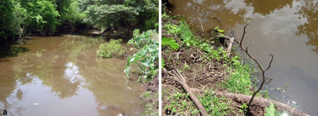
Figure 7. Habitat of Trifurcitus mexicanus sp. nov., in La Concordia Chiapas, México.
Abdomen: glossy black, with a slight reddish-yellow semicircular macule on the lateral margin of ventrites III to V; a slight lateral depression in ventrites II to VI, slightly deeper and expanded in ventrites V and VI; suture between ventrites I and II clearly marked; surface of ventrite II with faint parallel wrinkles on distal margin; ventrite III with few and tiny punctures in the center and parallel wrinkles in the distal region; ventrite IV without apparent puncture, but with scattered faint surface striae; ventrite V with a transverse line of few punctures and elongated wrinkles that do not reach the lateral depression; ventrite VI with uniformly rounded apex; with a slight transverse depression, and with lateral depression surrounded by slight striae, with scattered small subapical punctures. Setiferous punctuation with very short yellowish setae. Legs: fore and middle legs dark yellowish reddish, hind legs black, with pale reddish trochanter at apical half. Fore and middle legs dark yellowish reddish, hind legs black, with pale reddish trochanter at apical half. Protarsomere I with numerous tiny sucking setae at base and a row of large sucking setae at apex; protarsomere II with only 1 row of large sucking setae; protarsomere III with 2 rows of large sucking setae; protarsomere V with a pair of long, black, curved, sharp claws, the anterior 1 longer and thicker. Mesotarsomeres dark. Mesotarsomeres I-IV with a series of setae near the apical margin (posteroventrally); mesotarsomeres I-II with abundant ventral rows of long pale-yellow setae. Claws sharp and curved, the anterior 1 longer and thicker; both longer and thicker than the protarsal claws. Metafemur with rounded dorso-distal angle, weakly acute (almost straight), not pointed. Metatibiae with 2 apical spurs, the outer 1 noticeably thinner than the inner one, with trifid apex. Last metatarsomere with 2 straight and sharp claws of equal length, the outer 1 slightly wider. Male genitalia (Fig. 8c-f): parameres and median lobe; c-e) medial lobe in lateral, ventral and almost lateral (oblique) views; f) paramere in lateral view. c) Median lobe in lateral view (4.23 mm), and median sclerite (2.25 mm); d) median lobe in ventral view (maximum width 0.53 mm); e) median lobe in oblique ventrolateral view (4.26 mm), and median sclerite (3 mm); distance between median sclerite and apex of lobe 1.23 mm; f) left paramere (3.98 mm), with row of external ridges; the ridges reaching the ventral margin in the apical 3/3 (depending on the angle of inclination), simulate small teeth.
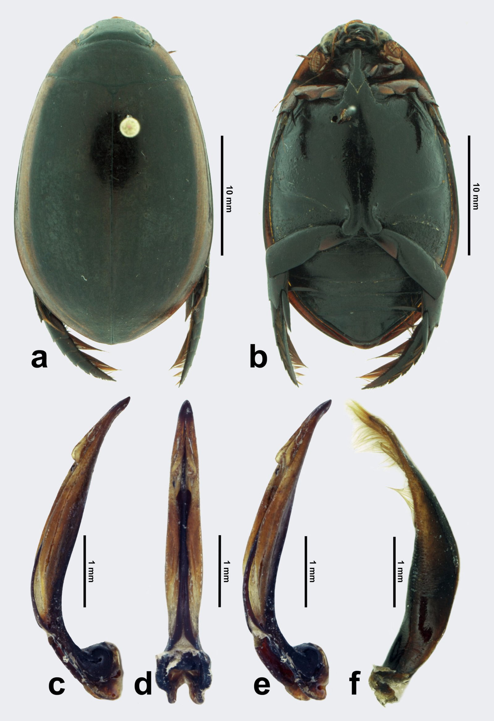
Figure 8. Habitus and genitalia of Trifurcitus maya sp. nov. a, b, Dorsal and ventral view of the habitus; c-e, lateral, ventral and oblique view of the middle lobe; f, lateral view of left paramere.
Variation. Paratype small. Length 27.5 mm, width 14.5 mm, dorsal and ventral punctures slightly smaller (less obvious). Median lobe in lateral view 4.15 mm; in ventral view, with maximum width 0.50 mm, and median sclerite 2 mm; ventrolateral (oblique) 4.20 mm, and median sclerite 2.95 mm; distance between the median sclerite and the apex of the lobe 1.20 mm; left paramere with row of external ridges, 3.95 mm; the ridges that reach the ventral margin in the apical 3/3 simulate small teeth. Another male from Mexico: total length 28.5 mm, width 14.5 mm. Dorsal and ventral punctuations slightly smaller (less evident). Median lobe in ventral view 4.20 mm, with maximum width 0.51 mm, and median sclerite 2.95 mm. Left paramere with row of external ridges 3.95 mm.
Taxonomic summary
Type locality: Mexico, Yucatán, km 90, ruta 295, Río Lagartos, 21°31’ N, 88°08’ W, elevation 10 m asl.
Type material: holotype (♂, IEXA): “Mexico: Yucatán/21°31’ N, 88°08’ W, 18-vi-1985/Col.: H. Velasco” [typed, white label], “holotype/Trifurcitus maya nov. sp./Arce-Pérez & Fery 2024” [typed, red label] (CNIN). Paratypes: 1 ♂, same data as holotype (CNIN), and 1 ♂ without precise location (collected in Mexico) (BMNH). Both paratypes with the following label: “paratype/Trifurcitus maya nov. sp./Arce-Pérez & Fery 2024” [typed, yellow label].
Distribution: this species is known from northern Yucatán, but it is very likely that it is also distributed in Quintana Roo and Campeche, between the states of the Gulf of Mexico and Yucatán.
Etymology: the specific name “maya” is assigned because it is the first record of the genus Trifurcitus for the region where the indigenous Maya people originated and developed in Mexico.
New state records:the giant diving beetle Bifurcitus lherminieri (Guérin-Méneville, 1829) is widely distributed in Mexico, recorded for the states of Campeche, Chihuahua, Jalisco, Oaxaca, Quintana Roo, Sinaloa, Veracruz and Yucatán, at elevations up to 1,480 m asl in cloud forests and temperate forests (Arce-Pérez & Reynoso-Velasco, 2022). It is now reported for the first time for the state of Nayarit, Tepic, 28-xi-1989, A. Cadena col. 1♂; and with reservation for the states of Guerrero, Acapulco, 5-xi-1970, J. Hendrichs col. (junto al mar) (1♀) and Tabasco, Villa Hermosa, Macultepec, 15/30-iv-1953, J. Hendrichs col. (1♀); Tonalá, Chico Zapote, 10-x-1953, J. Hendrichs col. (1♀) (CNIN).
Discussion
The fact that only 4 specimens of the genus Trifurcitus have been found in Mexico, a few others in South America and very few in the most important collections in the world, confirms what Miller (2013: 401) stated: “It is an interesting feature of dytiscid systematics that often the largest species are among the lesser-known taxa, while many of the smaller dytiscids have been revised using modern methods” (see also Short and McIntosh [2015: 671] for members of the family Hydrophilidae, and Arce-Pérez et al. [2021: 331] for other members of Cybisterinae, Dytiscidae). This also highlights the lack of collection activities (e.g. by using bottle traps as explained in Hendrich et al. [2019: 530] and faunal studies in aquatic environments in Mexico, as well as the need to restore, conserve and protect water bodies in various ecosystems in protected areas (and to the extent possible also in non-protected areas) to ensure the permanence of these beetles and other aquatic invertebrates.
Finally, it is evident that there is a need to review the material stored in collections under the generic names of Bifurcitus, Cybister, Metaxydytes (previously Megadytes and Cybister) to detect whether specimens of Trifurcitus mexicanus sp. nov., or Trifurcitus maya sp. nov. and other undescribed species may be hidden among them.
Acknowledgments
We thank the curators who kindly provided images, specially to Juan Carlos Urcola (University of Buenos Aires), and additional information: Santiago Zaragoza Caballero and Cristina Mayorga (CNIN); Pablo Mulieri and Gastón Zubarán (MACN), Sonia Casari and Gabriel Biff (MZSP), Michael Balke (ZSM) and Keita Matssumoto, Michael Geiser, and Max Barclay (BMNH). Special thanks to Daniel Reynoso-Velasco (INECOL), who donated the male from Chiapas and provided information and photos of the collecting site. Eder M. Mora (INECOL) took the photographs of the Mexican specimens. Finally, thanks to Emmanuel Arriaga Varela (INECOL) and an anonymous reviewer for their insightful comments to improve the work.
References
Arce-Pérez, R., Novelo-Gutiérrez, R., & Fery, H. (2021). Cybister (s. str.) poblanus sp. n. from Mexico and notes on other species of Cybistrinae (Coleoptera: Dytiscidae). Zootaxa, 5061, 323–339. https://doi.org/10.11646/zootaxa.5061.2.5
Arce-Pérez, R., & Reynoso-Velasco, D. (2022). New state records for Megadytes lherminieri (Guérin-Méneville, 1829) (Coleoptera: Dytiscidae: Cybistrinae) in Mexico. Proceedings of the Entomological Society of Washington, 124, 359–361. https://doi.org/10.4289/0013-8797.124.2.359
Aubé, C. (1838). Species général des hydrocanthares et gyriniens; pour faire suite au species général des coléoptères de la collection de M. le comte Dejean. París: Méquignon Père et Fils.
Brinck, P. (1945). Nomenklatorische und systematische studien über Dytisciden, III. Die Klassifikation der Cybisterinen. Kungliga Fysiografiska Sällskapets Handlingar, 56, 1–20.
Dejean, P. F. M. A. (1836). Catalogue des coléoptères de la collection de M. le comte Dejean. Ed. 3. París: Méquignon-Marvis.
Ferreira, Jr. N. (1995). Description of the larvae of Megadytes fallax (Aubé) and M. marginithorax (Perty) (Coleoptera: Dytiscidae). The Coleopterists Bulletin, 49, 313–318.
Hendrich, L., Manuel, M., & Balke, M. (2019). The return of the Duke-locality data for Megadytes ducalis Sharp, 1882, the world’s largest diving beetle, with notes on related species (Coleoptera: Dytiscidae). Zootaxa, 4586, 517–535. https://doi.org/10.11646/zootaxa.4586.3.8
Libonatti, M. L., Michat, M. C., & Torres, P. L. M. (2013). Aquatic Coleoptera from two protected areas of the humid Chaco eco-region (Chaco Province, Argentina). Revista de la Sociedad Entomológica Argentina, 72, 155–168.
Michat, M. C. (2010). Descriptions of larvae of Megadytes (Coleoptera: Dytiscidae: Dytiscinae): the subgenera Trifurcitus and Megadytes s. str., ground plan of chaetotaxy of the genus and phylogenetic analysis. European Journal of Entomology, 107, 377–392. https://doi.org/10.14411/eje.2010.047
Miller, K. B. (2013). Review of the genus Cybister Curtis, 1827 (Coleoptera: Dytiscidae: Dytiscinae: Cybistrini) in North America. The Coleopterists Bulletin, 67, 401–410. https://doi.org/10.1649/0010-065X-67.4.401
Miller, K. B., & Bergsten, J. (2016). Diving beetles of the World: systematics and biology of the Dytiscidae. Baltimore, Maryland: Johns Hopkins University Press.
Miller, K. B., Michat, M. C., & Ferreira, Jr. N. (2024). Reclassification of Cybistrinae Sharp, 1880 in the Neotropical Region (Coleoptera, Adephaga, Dytiscidae), with description of new taxa. Zookeys, 1188, 125–168. https://doi.org/10.3897/zookeys.1188.110081
Nilsson, A. N., & Hájek, J. (2023). A world catalogue of the family Dytiscidae (Coleoptera, Adephaga). Internet version 1.I. 2023. Retrieved on June 20, 2024 www.waterbeetles.eu
Sharp, D. (1882a). On aquatic carnivorous Coleoptera or Dytiscidae. Scientific Transactions of the Royal Dublin Society, Series II, 2, 179–1003.
Sharp, D. (1882b). Biologia Centrali-Americana. Zoologia. Insecta. Coleoptera. Vol. 1. Part 2. London: R. H. Porter.
Short, A. E. Z., & McIntosh, C. E. (2015). Hydrophilus harpe sp. nov., a remarkable new species of giant water scavenger beetle from Brazil (Coleoptera: Hydrophilidae). Acta Entomologica Musei Nationalis Pragae, 55, 665–671.
Trémouilles, E. R. (1984). Notas sobre Coleoptera acuáticos neotropicales. I. Cybister (Meganectes) parvus sp. nov. del Brasil (Coleoptera, Dytiscidae). Revista de la Sociedad Entomológica Argentina, 43, 187–190.
Trémouilles, E. R. (1989a). Notas sobre Coleoptera acuáticos neotropicales. II. Nuevos aportes al conocimiento del género Megadytes Sharp (Coleoptera, Dytiscidae), sobre ejemplares del British Museum (Natural History). Revista de la Sociedad Entomológica Argentina, 45, 153–157.
Trémouilles, E. R. (1989b). Notas sobre Coleoptera acuáticos neotropicales. III. Datos ampliatorios sobre distribución geográfica de especies de Megadytes Sharp (Coleoptera, Dytiscidae). Revista de la Sociedad Entomológica Argentina, 45, 159–161.
Trémouilles, E. R., & Bachmann, A. O. (1980). La tribu Cybisterini en la Argentina (Coleoptera, Dytiscidae). Revista de la Sociedad Entomológica Argentina, 39, 101–125
Wilke, S. (1920). Beiträge zur Kenntnis der Gattung Cybister Curtis. Archiv für Naturgeschichte, Abteilung, 85A,
243–276.
Zimmermann, A. (1920). Dytiscidae, Haliplidae, Hygrobiidae, Amphizoidae. In S. Schenkling (Ed.), Coleopterorum Catalogus, Volumen IV. Berlín: Junk.

A new species of Heteromyoxyuris (Nematoda: Oxyuridae), parasite of Dipodomysspp. (Rodentia: Heteromyidae) from Mexico
Una nueva especie de Heteromyoxyuris (Nematoda: Oxyuridae), parásito de Dipodomys spp. (Rodentia: Heteromyidae) de México
Jorge Falcón-Ordaz a, Jesus A. Fernandez b, Whitney Preisser c, Elizabeth A. Martínez-Salazar d, *
a Universidad Autónoma del Estado de Hidalgo, Laboratorio de Morfología Animal, Ciudad Universitaria, Carretera Pachuca Tulancingo s/n Km. 4.5, 42184 Mineral de la Reforma, Hidalgo, Mexico
b Universidad Autónoma de Chihuahua, Facultad de Zootecnia y Ecología, Departamento de Recursos Naturales, Periférico Francisco R. Almada Km. 1, 31453 Chihuahua, Chihuahua, Mexico
c Kennesaw State University, Department of Ecology, Evolution, and Organismal Biology, 370 Paulding Ave NW SC 326, MD 1202, Kennesaw, GA, 30144, USA
d Universidad Autónoma de Zacatecas, Unidad Académica de Ciencias Biológicas, Laboratorio de Colecciones Biológicas y Sistemática Molecular, Av. Preparatoria s/n, Campus Universitario II, Col. Agronómica, 98066 Zacatecas, Zacatecas, Mexico
*Corresponding author: eamskandii@gmail.com (E.A. Martínez-Salazar)
Received: 14 November 2024; accepted: 29 May 2025
http://zoobank.org/urn:lsid:zoobank.org:pub:51B9D39E-8714-4DC7-B17A-19CDCF1A1CE3
Abstract
A new species of Heteromyoxyuris, parasitic on the caecum of Dipodomys merriami and Dipodomys ordii from the Mexican Plateau, is described and illustrated. This species differs from the other 3 species by the absence of lateral alae in both sexes and resembles males of Heteromyoxyuris deserti by the presence of a pair of caudal cuticular inflations. The distribution of the 4 species of Heteromyoxyuris coincides with the geographical distribution of the heteromyid rodent subfamilies Dipodomyinae and Perognathinae across the deserts and arid lands of USA and Mexico. A key to the species of Heteromyoxyuris is provided. Heteromyoxyuris garciaprietoi n. sp. is the fourth species described for the genus and the second described for Mexico.
Keywords: Chihuahua; Guanajuato; Semi-arid regions; Heteromyoxyuris garciaprietoi n. sp.; Dipodomys spp.; Parasites
Resumen
En el presente estudio, una especie nueva del género Heteromyoxyuris, parásita del ciego intestinal de Dipodomys merriami y Dipodomys ordii del Altiplano mexicano se describe e ilustra. Esta especie se diferencia de las otras especies por la ausencia de alas laterales en ambos sexos y se asemeja a los machos de Heteromyoxyuris deserti por la presencia de 1 par de inflaciones cuticulares en la región caudal. La distribución del género Heteromyoxyuris coincide con la distribución de las subfamilias de roedores heterómidos Dipodomyinae y Perognathinae en los desiertos y tierras áridas de EUA y México. Se presenta una clave para las especies del género Heteromyoxyuris. Heteromyoxyuris garciaprietoi n. sp. es la cuarta especie del género y la segunda descrita para México.
Palabras clave: Chihuahua; Guanajuato; Regiones semiáridas; Heteromyoxyuris garciaprietoi n. sp.; Dipodomys spp.; Parásitos
Introduction
The genus Dipodomys (Heteromyide: Dipodomyinae) includes 20 species of kangaroo rats occurring throughout the arid and semi-arid regions of western North America, including both warm and cold deserts, grasslands, and chaparral, reaching semi-desert habitat at the Tehuacán–Cuicatlán Valley of southern Puebla and northern Oaxaca, Mexico (Alexander & Riddle, 2005; Fernández et al., 2012, 2014).
Ten valid species of Dipodomys have been recorded in Mexico (Fernández et al., 2014); however, their parasitic helminths have been neglected. To our knowledge, Dipodomys merriami Mearns, 1890, Dipodomys ordii Woodhouse 1853, and Dipodomys phillipsi Gray, 1841 are hosts of 2 species of cestode and 10 species of nematodes; it is noteworthy that the specific composition of these parasite communities varies among the 3 host species (further details on their parasites can be found in Preisser & Falcón-Ordaz, 2019). Notably, these 3 kangaroo rat species ecogeographically coincide within the tropical subtropical desert environment North and Central American ecosystems; D. merriami and D. phillipsii are exclusively inhabitants of the tropical and subtropical desert. In contrast, D. ordii is found in this ecoregion and extends its range to include the temperate steppe, temperate desert, and tropical and subtropical steppe (Alexander & Riddle, 2005).
To date, Heteromyoxyuris Quentin, 1973 (Nematoda: Oxyuridae) is distributed in deserts and arid lands of North America (Table 1), and comprises 3 species: Heteromyoxyuris deserti (Read and Millemann, 1953), with a primary distribution in the Chihuahuan Desert (localities detailed in Table 1); Heteromyoxyuris longejector (Hannum, 1943), found mainly in the Mexican Plateau; and Heteromyoxyuris otomii García-Prieto, Falcón-Ordaz, Lira-Guerrero, and Mendoza-Garfías, 2008, which is endemic to the Mexican Plateau. Within the family Heteromyidae, 3 rodent genera —Chaetodipus (pocket mice), Dipodomys (kangaroo rats), and Perognathus (silky pocket mice— are parasitized by these species of nematodes (García-Prieto et al., 2008; Table 1). Heteromyoxyuris longejector is the most widely distributed species in Mexico (Martínez-Salazar et al., 2016; Iturbe-Morgado et al., 2017), although both H. longejector and H. otomii have been found parasitizing 3 genera across the country (Table 1).
During a monitoring of Heteromyid rodent helminth parasites in the Mexican Plateau, many nematodes of an undescribed Heteromyoxyuris species were found in the caecum of D. merriami and D. ordii. The aim of this study is to describe a new species of the mentioned genus. In addition, a key to the species of Heteromyoxyuris is provided.
Materials and methods
In December 2015, 4 D. merriami and 1 D. ordii were trapped and collected in Sherman live-trap and subsequently euthanized following the standard procedures and techniques of the guidelines of the American Society of Mammologists (Kelt et al., 2010; Sikes & The Animal Care and Use Committee of the America Society of Mammalogists, 2016), under permit FAUT-0306 (issued to JAF), from 4.6 km S Ejido Mayran (25º37’48” N, 102º50’5.1” W; 1,091 m asl), municipality of San Pedro de las Colonias, Coahuila, Mexico. The viscera of the rodents were taken out and were fixed in 4% formalin. Intestinal samples were examined for helminths in June 2019. The skins and skulls of the specimens were deposited in the Colección de Mamíferos of the Universidad Autónoma de Chihuahua (UACH-M), with the numbers UACH-M152 for D. ordii and UACH-M153 for D. merriami.
In addition, specimens of Heteromyoxyuris sp. isolated from D. merriami and deposited at the Colección Nacional de Helmintos (CNHE), Instituto de Biología, Universidad Nacional Autónoma de México (IB-UNAM), Mexico City, Mexico, were examined. The nematodes were obtained from the caecum of the host and stored in 70% ethanol. The specimens were cleared on temporary slides by an immersion in a solution of glycerol and 70% ethanol (2:1). Transverse sections were made at different levels of the body in both sexes using a razor blade and placed in semi-permanent preparations. Photographs and measurements were taken using a Zeiss microscope, which was equipped with an Axiocam ERc5s and a calibrated ocular millimeter. For scanning electron microscopy (SEM) observations, 4 males and 4 females (2 of each sex per locality; these specimens were previously measured in the morphological study and correspond with the paratype series) were dehydrated in a series of graded ethanol solutions, followed by critical point drying with carbon dioxide. Six specimens (3 from Coahuila and 3 from Guanajuato) were coated with a gold-palladium mixture and examined in a Hitachi S-2460 N SEM (Hitachi, Tokyo, Japan) at 15 kV.
Table 1
Distribution of the genus Heteromyoxyuris in deserts and arid lands of North America (DALNA).
| Species | Host | Locality and Country | DALNA* | Reference |
| H. deserti | Dipodomys deserti | Lincoln County, Nevada, USA | MD | Quentin, 1973 |
| King & Babero, 1974 | ||||
| D. merriami | Victorville, California, USA | SD | Read & Millemann, 1953 | |
| Lincoln County, Nevada, USA | MD | King & Babero, 1974 | ||
| Quentin, 1973 | ||||
| Socorro County, New Mexico, USA | ChD | Decker et al., 2001 | ||
| Otero County, New Mexico, USA | ChD | Fedynich et al., 2001 | ||
| Dipodomys heermanni morroensis (Merriam, 1907) | Morro Bay, California, USA | ODA | Read & Millemann, 1953 | |
| D. ordii | Ward County, Texas, USA | ChD | Garner et al., 1976 | |
| Socorro County, New Mexico, USA | ChD | Decker et al., 2001 | ||
| Dipodomys panamintinus (Merriam, 1894) | Palmdale, California, USA | SD | Read & Millemann, 1953 | |
| D. spectabilis | Socorro County, New Mexico, USA | ChD | Decker et al., 2001 | |
| Perognathus flavus | Socorro County, New Mexico, USA | ChD | Decker et al., 2001 | |
| H. longejector | Chaetodipus sp. | Loreto, Zacatecas, Mexico | MP | Martínez-Salazar et al., 2016 |
| Pánuco, Zacatecas, Mexico | MP | Martínez-Salazar et al., 2016 | ||
| Villa de Cos, Zacatecas, Mexico | MP | Martínez-Salazar et al., 2016 | ||
| Ch. eremicus | Mazapil, Zacatecas, Mexico. | MP | Iturbe-Morgado et al., 2017 | |
| Ch. hispidus | Hidalgo, Durango, Mexico | MP | Iturbe-Morgado et al., 2017 | |
| San Luis de La Paz, Guanajuato, Mexico | MP | Iturbe-Morgado et al., 2017 | ||
| Villa de Reyes, San Luis Potosí, Mexico | MP | García-Prieto et al., 2008 | ||
| D. merriami | Arizona, USA | UNK | Hannum, 1941 | |
| Washington County, Utah, USA | CP | Bienek & Klikoff, 1974 | ||
| Pánuco, Zacatecas, Mexico | Martínez-Salazar et al., 2016 | |||
| Villa de Cos, Zacatecas, Mexico | MP | Martínez-Salazar et al., 2016 | ||
| Mazapil, Zacatecas, Mexico | MP | Iturbe-Morgado et al., 2017 | ||
| Perognathus sp. | Clark County, Nevada, USA | MD | Quentin, 1973 | |
| P. amplus | Mazatán, Sonora, Mexico | SD | García-Prieto et al., 2008 | |
| Perognathus californicus Merriam, 1889 | Monterrey, California, USA | ODA | Quentin, 1973 | |
| Table 1. Continued | ||||
| Species | Host | Locality and Country | DALNA* | Reference |
| Peromyscus sp. | Ojo Caliente, Zacatecas, Mexico | MP | Martínez-Salazar et al., 2016 | |
| Sylvilagus floridanus | Payne County, Oklahoma, USA | ODA | Boggs et al., 1990 | |
| H. otomii | P. flavus | San Luis de La Paz, Guanajuato, Mexico | MP | Iturbe-Morgado et al., 2017 |
| Ajacuba, Hidalgo, Mexico | MP | García-Prieto et al., 2008 | ||
| H. garciaprietoi n.sp. | D. merriami | San Luis de La Paz, Guanajuato, Mexico | MP | Iturbe-Morgado et al., 2017 |
| D. merriami | San Pedro de las Colonias, Coahuila, Mexico | MP | this study | |
| D. ordii | San Pedro las Colonias, Coahuila, Mexico | MP | this study |
*Mexican Plateau (MP); Great Basin Desert (GBD); Mohave Desert (MD); Sonora Desert (SD); Outside desert areas (ODA); Chihuahua Desert (ChD); Unknown (UNK); Colorado Plateau (CP).
The species description is based on specimens parasitizing 2 species of Dipodomys (D. ordii and D. merriami) from the states of Coahuila and Guanajuato; measurements of D. merriami specimens collected in Coahuila and Guanajuato are provided in Table 2. All measurements are given in micrometers (µm), unless otherwise indicated. The measurements are reported as a range, with the mean and standard deviation in parentheses. Also, the measurements of the holotype and allotype are included in brackets. The specimens were deposited in the CNHE, IB-UNAM.
Description
Family Oxyuridae Cobbold, 1864
Genus Heteromyoxyuris Quentin, 1973
Heteromyoxyuris garciaprietoi n. sp. Falcón-Ordaz and Martínez-Salazar
(Figs. 1-3)
http://zoobank.org/urn:lsid:zoobank.org:act:716F4F32-F0BE-473C-95AB-7297A8635510
General description (based on 57 individuals, 17 males and 40 females). Nematodes small and robust. Mouth with 3 strong teeth (Fig. 1A); females with 3 interlabial processes, 2 latero-dorsal and 1 ventral (Fig. 1B). Cephalic end with 2 circles of 4 papillae each; external circle simple papillae (Fig. 1C), clearly differentiated; amphids located at external circle of papillae. Cephalic region separated from body by deep groove (Fig. 1D). Males with a pair of caudal cuticular inflations and tail acute (Fig. 1E). Females with conical tail. Excretory pore situated in first third of body. In cross sections at different levels of the body, lateral alae are not observed in either sex (Fig. 2A-F).
The measurements of the Dipodomys ordii specimens from Coahuila are given below, while those of Dipodomys merriami from Guanajuato and Coahuila are presented in Table 2.
Table 2
Measurements of paratype specimens (min.-max., mean ± standard deviation) of Heteromyoxyuris garciaprietoi n. sp., parasite of Dipodomys merriami from Guanajuato and Coahuila.
| Locality | San Luis de La Paz | San Pedro de las Colonias | ||
| State | Guanajuato | Coahuila | ||
| Sex | Male, n = 8 | Female, n = 16 | Male, n = 4 | Female, n = 8 |
| Length (mm) | 2.52-3.55 (3±0.34) | 7.30-12.45 (10.48±1.66) | 1.78-2.8 (2.5±0.5) | 9.1-11 (10.1±8) |
| Maximum diameter | 182.5-232.5 (218.12±17.81) | 265-472.5 (373.9±69.52) | 125-180 (159.3±26.3) | 360-455 (411.5±35.5) |
| Esophagus with bulb | ||||
| Length | 325-425 (381.25±32) | 550-725 (629.68±48.49) | 345-392.5 (372.5±20.1) | 570-630 606.2±21.3) |
| Esophageal bulb | ||||
| Length | 70-100 (89.37±10.66) | 100-162.5 (134.68±18.43) | 77.5-92.5 (82.5±7) | 110-132.5 (126.2±9) |
| Width | 72.5-120 (92.81±14.72) | 107.5-170 (141.25±19.4) | 72.5-90 (81.8±8.2) | 140-157.5 (150±6) |
| Nerve ring | 95-132.5 (113.43±11.72) | 130-370 (196.1±55.55) | 82.5-145 (105±28.3) | 165-195 (176.2±15.2) |
| Excretory pore | 177.5-870 (671±235.14) | 1.18-1.80 mm (1.48±0.22) | 215-350 (273.7±61.1) | 1.2-1.6 mm 1.4±0.12 |
| Spicule length | 77.5-80 (78.33±1.44) | 75-80 (77.5±3) | ||
| Gubernaculum length | 22.5-27.5 (24.5±2.09) | 25-27.5 (26.6±1.44) | ||
| Vulva | 3.0-4.8 mm (3.84±0.59) | 3.8-4.4 mm (4.1±0.22) | ||
| Ovejector | 300.0-620 (434.54±96.47) | 250-362.5 (318.4±38.2) | ||
| Anus* | 100-157.5 (129.64±20.12) | 0.85-1.47 mm (1.23±0.17) | 105-145 (126±20) | 0.96-1 mm (1±0.04) |
| Tail length | 70-127.5 (95.93±19.95) | 85-87.5 (86.2±1.4) | ||
| Caudal cuticular inflation | 70-127.5 (96±20) | 192.5-255 (221.8±28.3) | ||
| Eggs | ||||
| Length | 100-112.5 (107.63±4.23) | 97.5-112.5 (105.3±3.8) | ||
| Width | 30-40 (35.76±2.80) | 30-40 (34.2±2.4) |
*In male is cloaca and in females is anus.
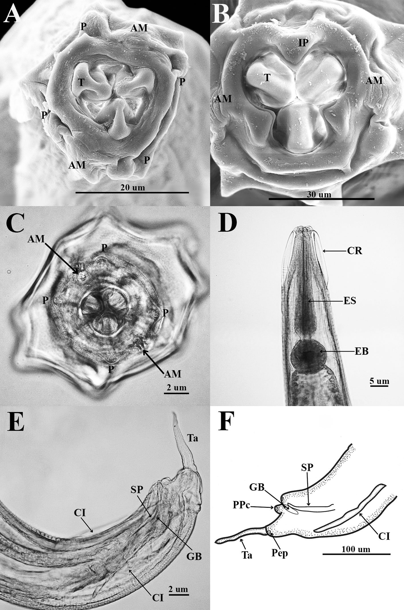
Figure 1. Heteromyoxyuris garciaprietoi n. sp., scanning electron micrographs. A, Male, apical view, amphids (AM), papillae (P), and tooth (T); B, female, apical view, interlabial processes (IP). Micrographs; C, male, apical view; D, lateral view of the cephalic region (CR), showing the esophagus (ES) and the esophageal bulb (EB); E, lateral view of the caudal region, showing cuticular inflation (CI), spicule simple (SP), gubernaculum (GB), and tail (Ta); F, line drawing of the caudal region, showing the same structures as in Figure (E), plus a pair of preanal papillae (PPc) and pedunculated papillae (Pep).
Male (based on holotype and 4 paratypes):body 2.9-3.7 (3.2±0.3) mm long and 202.5-222.5 (211±10.5) width at mid-body. Esophagus length 105-437.5 (351±139); esophageal bulb 95-110 (100.5±6.7) long and 92.5-120 (102.5±12) wide. Nerve ring and excretory pore located at 85-130 (108.5±17.2), and 490-567.5 (540.5±27), from anterior end, respectively. Spicule simple 75-82.5 (79.3±3.14) in length; gubernaculum 20-27.5 (24±3) long (Fig. 1E, F). Tail 127.5-137.5 (132±4.1) long; tail reduced to slender appendage 90-117.5 (100±16) in length. In the caudal region, the specimens exhibit a cuticular inflation 182.5-255 (207.5±17.5) long. Caudal sessile papillae arranged as follows: 1 preanal pair and 2 postanal pairs; posterior pair fused. One additional pair of pedunculated papillae located laterally at beginning of caudal filament containing phasmidia (Fig. 3A-C).
Female (based allotype and 15 paratypes):length 8.0-12.1 (11±1.4) mm, width 270-457.5 (386.2±0.7) at mid-body level. Esophagus length 590-680 (645±35.8); esophageal bulb 130-147.5 (139±7.7) long by 130-187.5 (158.1±20.6) wide. Nerve ring and excretory pore located at 125-207.5 (166.2±23), and 1.21-1.69 (1.4±0.1) mm from anterior end, respectively. Vulva opening at 3.1-5.3 (4.2±0.7) mm from anterior end. Ovejector 257.5-390 (338.7±44.7) long (Fig. 3D). Tail conical, 1.0-1.4 (1.1±0.1) mm long (Fig. 3E). Eggs without operculum, 97.5-112.5 (105.2±4.6) long by 30-40 36.3±3.2) wide (Fig. 3F).
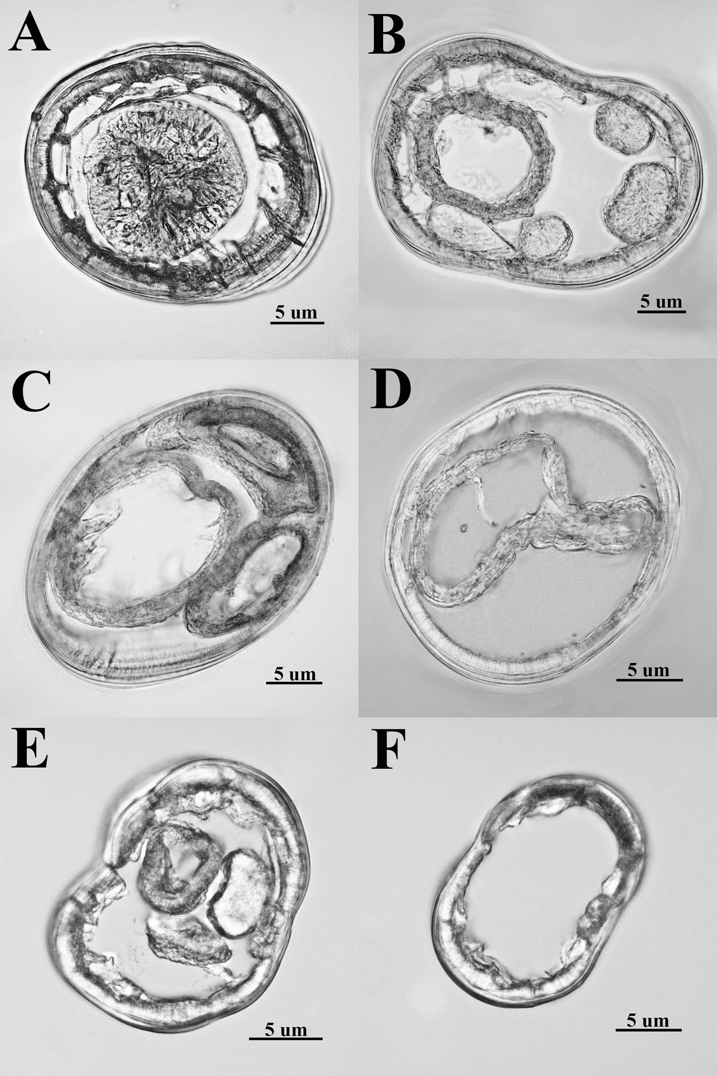
Taxonomic summary
Type host: Dipodomys ordii (UACH-M152)
Type locality: 4.6 km S Ejido Mayran (25º37’48” N 102º50’5.1” W; 1,091 m asl), municipality of San Pedro de las Colonias, Coahuila, Mexico.
Site of infection: intestinal caecum.
Type specimens: holotype male (CNHE 12143); allotype female (CNHE 12144); paratypes: 8 males and 4 females (CNHE 12145).
Etymology: the new species was named in honor of MSc. Luis García-Prieto (IB-UNAM, Mexico) for his important and invaluable contribution to Mexican parasitology.
Other hosts and localities: Dipodomys merriami, 4.6 km S Ejido Mayran, municipality of San Pedro de las Colonias, Coahuila, Mexico (CNHE 12146); 3 km N San Luis de La Paz, Guanajuato, Mexico (CNHE: 9832).
Remarks. Hereromyoxyuris was established by Quentin in 1973 and currently comprises 4 species: H. longejector, H. deserti, H. otomii (Quentin, 1973; García-Prieto et al., 2008), and H. garciaprietoi n. sp. The new species is characterized by the presence of 2 circles of 4 cephalic papillae (which are double in external circle), a mouth opening surrounded by 3 interlabia (1 ventral and 2 laterodorsals), containing 3 thick teeth, a strongly muscular vagina and nonembryonated eggs, lacking opercula. The new species is unique in that it is the only one with a smooth cuticle, not featuring lateral alae in worms of either sex. In contrast, H. deserti exhibits simple lateral alae located on both sides of the body. The males of both H. deserti and the new species feature caudal alae (caudal cuticular inflation) on the caudal region. These alae are more prominent in H. deserti (Fig. 4, in Quentin, 1973) than in the new species. In comparison to the new species, both H. longejector and H. otomii possess double alae on both sides of the body. The new species is found in 2 localities of the Mexican Plateau, where it parasitizes 2 species of the genus Dipodomys.
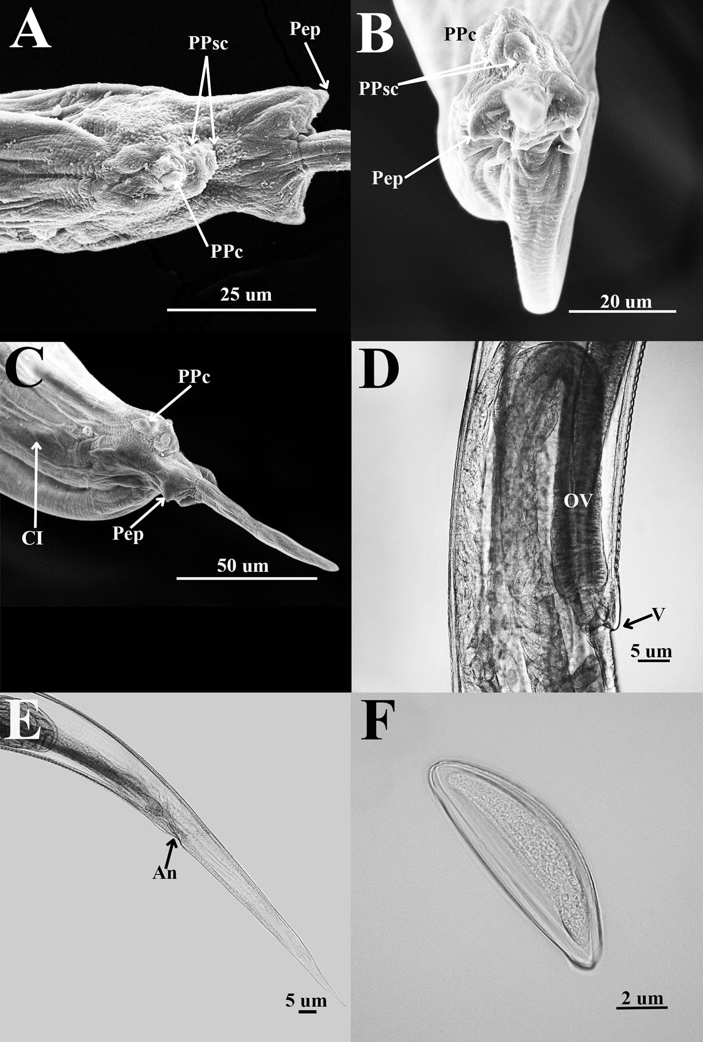
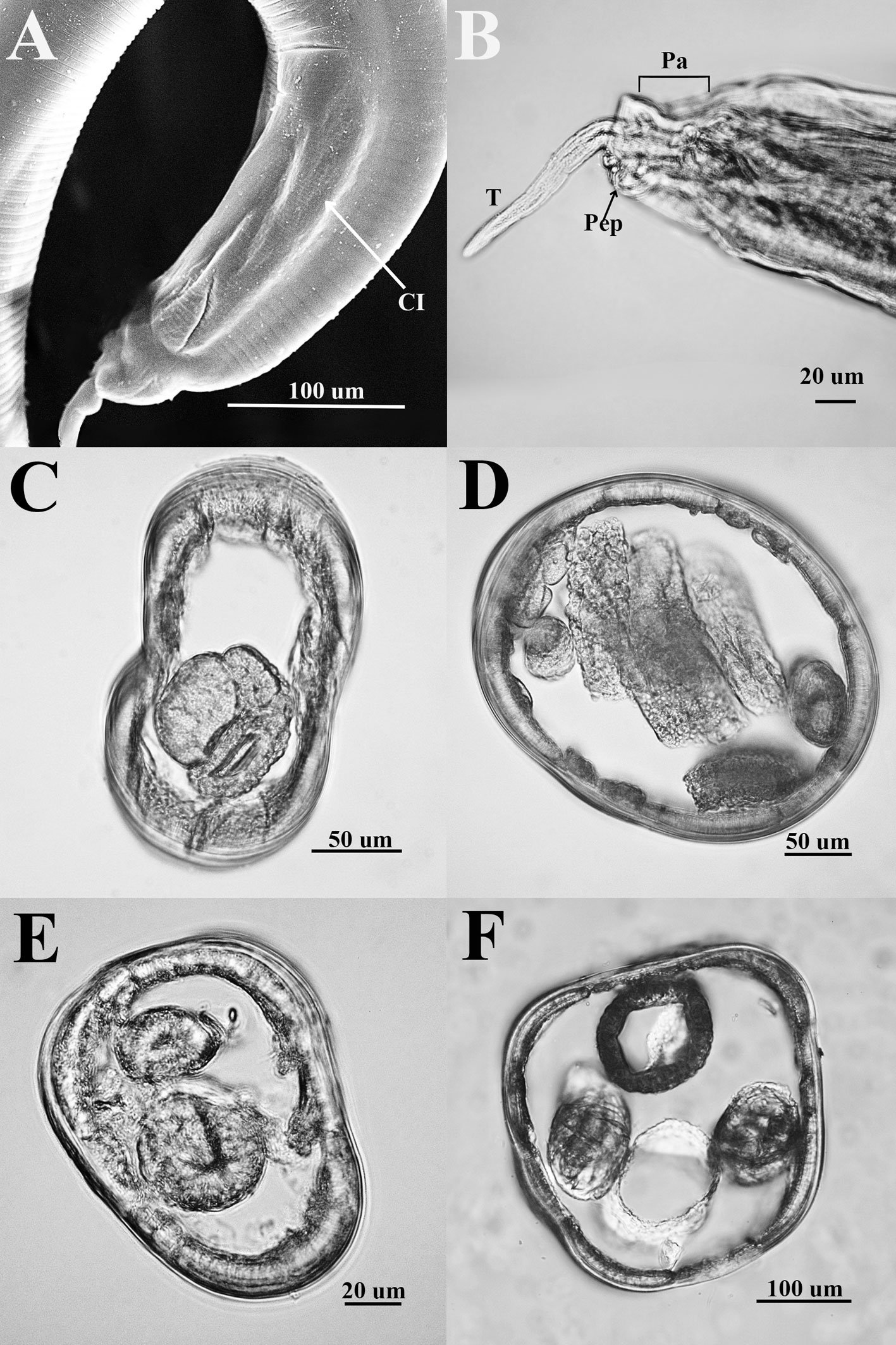
Also, the morphometry of specimens from Guanajuato and Coahuila is consistent with the same morphological characteristics (Table 2). Notably, the males present a caudal cuticular inflation (Fig. 4A); the arrangement of the papillae in the caudal region is the same as that described above (Fig. 4B). Both sexes lack lateral alae (Fig. 4 C-E).
The distribution of the genus Heteromyoxyuris coincides with the geographic distribution of the heteromyid rodent subfamilies Dipodomyinae (6 species) and Perognathinae (7 species) (Morrone, 2005; Omernik, 1987). Despite a record of H. longejector in Sylvilagus floridanus (J. A. Allen, 1890) (Lagomorpha: Leporidae] from Oklahoma, USA, this finding remains unverified due to the absence of a voucher specimen [therefore, we have excluded this data from our work; Boggs et al., 1990]).
Biogeographic studies of North American and Mexican deserts and drylands frequently reveal an east-west division of closely related species, with sister species often limited to the eastern (Chihuahuan) and western (Mojave and Sonoran) deserts (Ayoub & Riechert, 2004; Devitt, 2006; Douglas et al., 2006; Jaeger et al., 2005; Wilson & Pitts, 2010). The distribution pattern observed is presumably present in the Heteromyoxyuris host-parasite system. To confirm our hypothesis of a mirrored distribution pattern, initially we need to undertake phylogenetic analyses and exploratory studies in regions that match the host distribution.
In Mexico, Heteromyoxyuris has been found in Coahuila, Durango, Guanajuato, San Luis Potosí, and Zacatecas (Table 1). Most records of this nematode genus are associated with Heteromyidae, including hosts such as Chaetodipus eremicus (Mearns, 1898), Chaetodipus hispidus (Baird 1858), Chaetodipus sp., Dipodomys merriami, Dipodomys ordii, Perognathus amplus Osgood, 1900, and Perognathus flavus Baird, 1855. Only 1 record exists in Cricetidae, specifically in Peromyscus sp. Heteromyoxyuris deserti and H. longejector are of particular interest for biogeographic studies due to their wide distribution across the deserts and drylands of North America. The evidence suggests that both H. longejector and H. deserti are generalist parasites, infecting a wide range of hosts: 9 and 7 species, respectively (Table 1). It is noteworthy that H. deserti has been documented in Nevada, California, New Mexico, and Texas, USA, as well as in host species that are also distributed in Mexico. These include Dipodomys deserti Stephens, 1887, D. merriami, D. spectabilis Merriam, 1890, D. ordii, and P. flavus (Table 1). Therefore, it cannot be excluded that this species is also present in arid and semi-arid regions of Mexico.
Heteromyoxyuris otomii and H. garciaprietoi n. sp. are currently endemic to Mexico, but their distribution could be as wide as that of their hosts, which are not endemic to Mexico. Heteromyoxyuris otomii has only been recorded on P. flavus in Guanajuato and Hidalgo, Mexico (García-Prieto et al., 2008; Iturbe-Morgado et al., 2017). However, since its host is widespread across central Mexico and the southern USA, this species of nematode likely occurs in other regions in Mexico. Likewise, the broad distribution of D. merriami and D. ordii suggests that H. garciaprietoi n. sp. probably exists in other Mexican locations, similar to H. longejector (Table 1).
So far, there is only 1 study of the parasites of rodents in Coahuila. According to Falcón-Ordaz et al. (2024), only D. merriami has been examined for parasites in Coahuila, reporting Syphacia sp., Pterygodermatites dipodomis Tiner, 1948, and Protospirura dipodomis (Read & Millemann, 1953), and H. garciaprietoi n. sp. The diversity of parasitic helminths in rodents remains incomplete (García-Prieto et al., 2012; Falcón-Ordaz et al., 2024; Iturbe-Morgado et al., 2017; Martínez-Salazar et al., 2016), and the helminth fauna is still unknown in Campeche, Quintana Roo, Sinaloa, and Tamaulipas (González-Moreno & Falcón-Ordaz, 2025) or is under investigation, as in the Baja California Peninsula (Martínez-Salazar, Pers. Comm.).
Conservation efforts often overlook parasites, despite their ecological significance and potential as environmental indicators (Lymbery & Smit, 2023). Bridging this knowledge gap demands comprehensive updates to taxonomic inventories; this means examining not just living wildlife, but also the extensive collections of parasite and host material housed in biological repositories, since there are still species to be discovered (e.g., Museomics, see Fernández, 2019; Greiman et al., 2018). In addition, some areas are inaccessible for various reasons or due to the lack of support directed to this type of work (Martínez-Salazar et al., 2016). Undoubtedly, our understanding of host-parasite systems is incomplete, largely due to significant gaps in knowledge of species diversity (the Linnaean shortfall), their distribution (the Wallace shortfall), and their phylogenetic and evolutionary relationships (the Darwin shortfall) (Hortal et al., 2015; Rubio-Godoy & Pérez-Ponce de León, 2023). To reduce these limitations, we examined the material deposited at the CNHE (CNHE 9832), and subsequently, taxonomic analysis revealed that this material corresponds to H. garciaprietoi n. sp. The examination of museum specimens, as evidenced by the discovery of H. garciaprietoi n. sp. in CNHE material, highlights the vital role of biological collections in this effort.
In this study, it was not possible to extract DNA from the H. garciaprietoi n. sp. material due to the fixation condition of the organs examined (in formalin). Therefore, if this species is found in other regions of the country, it may offer a favorable panorama for exploring the phylogenetic relationships of the genus. Regarding this last point, it would be essential to confirm the close morphological relationship that the new species has with H. deserti. Heteromyoxyuris garciaprietoi n. sp. is the only species of the genus that does not have lateral alae in either sex. This is the fourth species described for the genus and the second described for Mexico.
Key to species of the genus Heteromyoxyuris Quentin, 1973
1a. Male and female with lateral alae on the body 2a
1b. Male and female without lateral alae on the body H. garciaprietoi n. sp.
2a. Male and female with simple lateral alae on the body H. deserti (Read and Millemann, 1953)
2b. Male and female with double lateral alae on the body 3a
3a. The lateral alae extend from esophageal bulb to anus in both sexes H. otomii García-Prieto, Falcón-Ordaz, Lira-Guerrero and Mendoza-Garfías, 2008
3b. The lateral alae in male begin at the posterior half of the body and in female start posterior to esophageal bulb ending in the anus in both sexes H. longejector (Hannum, 1943)
Acknowledgements
We are indebted to Berenit Mendoza-Garfias for her invaluable assistance in processing samples for the SEM photographs in the Laboratorio de Microscopía y Fotografía de la Biodiversidad I, at the LANABIO (IB-UNAM) and Luis Garcia-Prieto for kindly loaning specimens of the CNHE (IB-CNHE). We also want to thank Mitzi F. Aquino-Camacho for editing the figures. The treating results were obtained as part of the project “Sistemática y taxonomía de helmintos parásitos de vertebrados con enfásis en pequeños mamíferos” (number UAEH-DI-17-ICBI-BI-SF-107, J. Falcón-Ordaz, main researcher), and were partially written during the project UAZ-2023-38899 (Elizabeth A. Martínez-Salazar, main researcher). We are grateful to the Associate Editor and the anonymous reviewers for their valuable suggestions for improvements to the manuscript.
References
Alexander, L. F., & Riddle, B. R. (2005). Phylogenetics of the new world rodent family Heteromyidae. Journal of Mammalogy, 86, 366–379. https://doi.org/10.1644/BER-120.1
Ayoub, N. A., & Riechert S. E. (2004). Molecular evidence for Pleistocene glacial cycles driving diversification of a North American desert spider, Agelenopsis aperta. Molecular Ecology, 13, 3453–3465. https://doi.org/10.1111/j.1365-294X.2004.02335.x
Bienek, G. K., & L. G. Klikoff, L. G. (1974). Parasitological evidence of arthropods as food for Dipodomys merriami vulcani. American Midland Naturalist, 91, 251–253. https://doi.org/10.2307/2424421
Boggs, J. F., McMurry, S. T., Leslie, Jr. D. M., Engle, D. M., & Lochmiller, R. L. (1990). Influence of habitat modification on the intestinal helminth community ecology of cottontail rabbit populations. Journal of Wildlife Diseases, 26, 157–169. https://doi.org/10.7589/0090-3558-26.2.157
Decker, K. H., Duszynski, D. W., & Patrick, M. J. (2001). Biotic and abiotic effects on endoparasites infecting Dipodomys and Perognathus species. Journal of Parasitology, 87, 300–307. https://doi.org/10.1645/0022-3395(2001)087[0300:BAAEOE]2.0.CO;2
Devitt, T. J. (2006). Phylogeography of the Western Lyresnake (Trimorphodon biscutatus): testing arid land biogeographical hypotheses across the Nearctic-Neotropical transition. Molecular Ecology, 15, 4387–4407. https://doi.org/10.1111/j.1365-294X.2006.03015.x
Douglas, M. E., Douglas, M. R., Schuett, G. W., & Porras, L. W. (2006). Evolution of rattlesnakes (Viperidae: Crotalus) in the warm deserts of western North America shaped by Neogene vicariance and Quaternary climate change. Molecular Ecology, 15, 3353–3374. https://doi.org/10.1111/j.1365-294X.2006.03007.x
Falcón-Ordaz J., Aquino-Camacho, M. F., Ladrón de Guevara-Bárcenas, K., & Fernández, J. A. (2024). Helminths parasites of heteromyd rodents from semiarid regions of Mexico. Therya Notes, 5, 157–161. https://doi.org/10.12933/therya_notes-24-164
Fedynich, A. M., Monasmith, T., & Demarais, S. (2001). Helminth community structure and pattern in Merriam’s kangaroo rats, Dipodomys merriami Mearns, from the Chihuahuan Desert of New Mexico, U.S.A. Comparative Parasitology, 68, 116–121.
Fernández, J. A. (2019). The holistic specimen and parasites of mammals. Therya, 10, 65–67. https://doi.org/10.12933/therya-19-827
Fernández, J. A., Cervantes, F. A., & Hafner, M. S. (2012). Molecular systematics and biogeography of the Mexican endemic kangaroo rat, Dipocomys phillipsii (Rodentia: Heteromyidae). Journal of Mammalogy, 93, 560–571. https://doi.org/10.1644/11-MAMM-A-224.1
Fernández, J. A., Hafner, M. S., Hafner, D. J., & Cervantes, F. A. (2014). Conservation status of rodents of the families Geomyidae and Heteromyidae of Mexico. Revista Mexicana de Biodiversidad, 85, 576–588. https://doi.org/10.7550/rmb.36710
García-Prieto, L., Falcón-Ordaz, J., & Guzmán-Cornejo, C. (2012). Helminth parasites of wild Mexican mammals: list of species, host and geographical distribution. Zootaxa, 3290, 1–92. https://doi.org/10.11646/zootaxa.3290.1.1
García-Prieto, L., Falcón-Ordaz, J., Lira-Guerrero, G., & Mendoza-Garfias, B. (2008). A new species of Heteromyoxyuris (Nematoda: Oxyuridae), parasite of Perognathus flavus (Rodentia: Heteromyidae) from Mexico. Journal of Parasitology, 94, 860–865. https://doi.org/10.1645/GE-1452.1
Garner, H. W., Richardson, L. W., & Felts, L. A. (1976). Alimentary helminths of Dipodomys ordii: effects on the host population. The Southwestern Naturalist, 21, 327– 334. https://doi.org/10.2307/3669718
González-Moreno, C. D., & Falcón-Ordaz, J. (2025). Análisis de la riqueza de helmintos en roedores de México. Pädi Boletín Científico de Ciencias Básicas e Ingenierías del ICBI, 12, 22–27. https://doi.org/10.29057/icbi.v12i24.12640
Greiman, S. E., Cook, J. A., Tkach, V. V., Hoberg, E. P., Menning, D. M., Hope, A. G. et al. (2018). Museum metabarcoding: a novel method revealing gut helminth communities of small mammals across space and time. International Journal for Parasitology, 48, 1061–1070. https://doi.org/10.1016/j.ijpara.2018.08.001
Hannum, C. A. (1941). Nematode parasites of Arizona vertebrates (Ph.D. Thesis). University of Washington, Seattle.
Hortal, J., Bello, F., Diniz-Filho, J. A., Lewinsohn, T. M., Lobo, J. M., & Ladle, R. J. (2015). Seven shortfalls that beset large-scale knowledge of biodiversity. Annual Review of Ecology, Evolution, and Systematics, 46, 523–549. https://doi.org/10.1146/annurev-ecolsys-112414-054400
Iturbe-Morgado, J. C., Falcón-Ordaz, J., Lira-Guerrero, G., Fernández, J. A., & Acosta, R. (2017). Nematofauna of rodents of the families Heteromyidae and Cricetidae from the Mexican Plateau. Journal of Parasitology, 103, 127–131. https://doi.org/10.1645/16-105
Jaeger, J. R., Riddle, B. R., & Bradford, D. F. (2005). Cryptic Neogene vicariance and Quaternary dispersal of the red-spotted toad (Bufo punctatus): insights on the evolution of North American warm desert biotas. Molecular Ecology, 14, 3033–3048. https://doi.org/10.1111/j.1365-294X.2005.02645.x
Kelt, D. A., Hafner, M. S., & The American Society of Mammalogists’ ad hoc Committee for Guidelines on Handling Rodents in the Field. (2010). Updated guidelines for protection of mammalogists and wildlife researchers from hantavirus pulmonary syndrome (hps). Journal of Mammalogy, 91, 1524–1527. https://doi.org/10.1644/10-MAMM-A-306.1
King, S. R., & Babero, B. B. (1974). Helminths of kangaroo rats (Dipodomys spp.) in Nevada with reports of other worm parasites from these hosts. Proceedings of the Helminthological Society of Washington, 41, 241–248.
Lymbery, A. J., & Smit, N. J. (2023). Conservation of parasites: a primer. International Journal for Parasitology: Parasites and Wildlife, 21, 255–263. https://doi.org/10.1016/j.ijppaw.2023.07.001
Martínez-Salazar, E. A., Flores-Rodríguez V., Rosas-Valdez, R., & Falcón-Ordaz, J. (2016). Helminth parasites of some rodents (Cricetidae, Heteromyidae, and Sciuridae) from Zacatecas, Mexico. Revista Mexicana de Biodiversidad, 87, 1203–1211. https://doi.org/10.1016/j.rmb.2016.10.009
Morrone, J. J. (2005). Hacia una síntesis biogeográfica de México. Revista Mexicana de Biodiversidad, 76, 207–252. http://dx.doi.org/10.22201/ib.20078706e.2005.002.303
Omernik, J. M. (1987). Ecoregions of the Conterminous United States. Annals of the Association of American Geographers, 77, 118–125. https://doi.org/10.1111/j.1467-8306.1987.tb00149.x
Preisser, W. C., & Falcón-Ordaz, J. (2019). A checklist of the parasitic helminths of cricetid and heteromyid rodents in Mexico. Therya, 10, 329–341. http://dx.doi.org/10.12933/therya-19-787
Quentin, J. C. (1973). Les Oxyurinae de Rongeurs. Bulletin du Muse ́e Nationalle d’Histoire Naturelle, 12, 1045–1096.
Read, C. P., & Millemann, R. E. (1953). Helminth parasites in kangaroo rats. University of California Publications in Zoology, 59, 61‒80.
Rubio-Godoy, M., & Pérez-Ponce de León, G. (2023). Equal rights for parasites: Windsor 1995, revisited after ecological parasitology has come of age. Biological Conservation, 284, 110174. https://doi.org/10.1016/j.biocon.2023.110174
Sikes, R. S., & The Animal Care and Use Committee of the American Society of Mammalogists. (2016). Guidelines of The American Society of Mammalogists for the use of wild mammals in research and education. Journal of Mammalogy, 97, 663–688. https://doi.org/10.1093/jmammal/gyw078
Wilson, J. S., & Pitts, J. P. (2010). Phylogeographic analysis of the nocturnal velvet ant genus Dilophotopsis (Hymenoptera: Mutillidae) provides insights into diversification in the Nearctic deserts. Biological Journal of the Linnean Society, 101, 360–375. https://doi.org/10.1111/j.1095-8312.2010.01526.x

Una especie nueva de Lippia (Verbenaceae:Lantanae) de la Sierra de La Giganta, Baja California Sur, México
A new species of Lippia (Verbenaceae: Lantanae) from the Sierra de La Giganta, Baja California Sur, Mexico
Jose Luis León-de la Luz
Centro de Investigaciones Biológicas del Noroeste, S.C., Apartado postal 128, 23000 La Paz, Baja California Sur, México
*Autor para correspondencia: pachycereus@gmail.com (J.L. León-de la Luz)
Recibido: 16 enero 2025; aceptado: 9 junio 2025
Resumen
Se describe e ilustra a Lippia domingeziorum, una especie nueva de Verbenaceae del extremo sur de la sierra La Giganta, península de Baja California, México. Actualmente, se conoce solo de los arroyos arenosos y rocosos en las estribaciones bajas del cerro Cabeza del Mechudo, en la bahía de La Paz. Este nuevo taxón parece ser cercano a L. palmeri, de quien se distingue porque su flor y la respectiva bráctea floral, son casi del doble de tamaño. Ambos taxones son simpátricos y comparten algunos rasgos, como las abundantes glándulas de aceite en el indumento, pero las de esta nueva especie carecen del típico aroma de orégano que distingue a L. palmeri. Se presentan una descripción botánica detallada e imágenes que ilustran al nuevo taxón. Las relaciones de parentesco de esta nueva especie dentro del género Lippia es aún incierta, pero estudios citogenéticos y moleculares futuros deben ayudar a resolver esta temática.
Palabras clave: Bahía La Paz; Biodiversidad; El Mechudo; Orégano
Abstract
We describe and illustrate Lippia domingeziorum, a new species of Verbenaceae from the southern tip of the Sierra La Giganta, Baja California peninsula, Mexico. Currently, it is known only from the rocky-sandy arroyos at the foothills of Cerro Cabeza del Mechudo in La Paz Bay. This novelty appears to be closely related to L. palmeri, which it distinguishes because its flower and corresponding floral bract are almost twice as large. Both taxa are sympatric and share some features, such as the abundant oil glands on the indumentum, but those of this new species lack the typical oregano scent that characterizes L. palmeri. A detailed botanical description and illustrations of this new taxon are presented. The relationships of this novelty within the genus Lippia is still in an open issue, but future cytogenetic and molecular insights might help to address this matter.
Keywords: La Paz Bay; Biodiversity; El Mechudo; Oregano
Introducción
El género Lippia L es uno de los más diversificados y complejos de la familia Verbenaceae J. St.-Hil. (tribu Lantaneae Endl.), que incluye un número todavía indefinido de taxones (120-160) arbustivos y subarbustivos, así como de herbáceas perennes, nativas del trópico americano (Atkins, 2004) aunque con algunos representantes en África (Cardoso et al., 2021); el este de Brasil concentra una notable diversidad de especies, con cerca de 90 (Lu-Irving et al., 2021). Debido a que muchos de sus taxones tienen un típico aroma, tienen uso como especias en la cocina, y también terapéutico.
Desde mediados de la década de los 90, el personal del herbario HCIB (Thiers, 2024) ha compilado detalladamente colectas botánicas en la Sierra de La Giganta, considerada como eje geológico de la mitad sur de la península de Baja California (noroeste de México), actividad que ha rendido varias publicaciones, como el análisis florístico de la región (León-de la Luz et al., 2008). Al mismo tiempo, la visita a diferentes puntos remotos de esta enorme cadena montañosa, permitió ampliar los registros florísticos de la zona, así como contribuir a la conservación de especies vegetales, localizando taxones previamente no reportados, raros, e incluso no descritos (León-de la Luz y Domínguez, 2006; León-de la Luz y Rebman, 2010), atrayendo la atención de agencias de conservación no-gubernamentales, y a la autoridad ambiental de México, al ofrecer informes de la flora y vegetación de las zonas exploradas. Esto ha permitido que esta serranía este hoy día considerada para su designación como un área natural protegida (Conanp, 2014).
Durante las exploraciones botánicas en el extremo sur de la Sierra de La Giganta, dentro de la bahía de La Paz, se colectaron interesantes ejemplares de Lippia en 2001, 2005 y 2015 (Miguel Domínguez 3049, 16776 HCIB; José Luis León 10390; 20214 HCIB; Raymundo Domínguez 4336, 30023 HCIB), aunque su completa identidad había estado pendiente, hasta recientemente. A primera impresión, su morfología parece ser una variación de la bien conocida especie de “orégano de monte” Lippia palmeri S. Watson (1889: 67), para algunos autores incluida dentro de Lippia origanoides Kunth (1818: 267), ya que ambos taxones presentan, entre otros caracteres, inflorescencias espigadas, con flores sésiles a lo largo del eje central.
Al término de lluvias generosas que se presentaron en esta región geográfica durante octubre de 2023, se visitó la zona de las estribaciones del cerro Cabeza del Mechudo. En diciembre se encontró una vigorosa población de decenas de individuos en floración plena y en el mismo lugar, algunas plantas de Lippia palmeri también en floración, lo cual resolvió la duda sobre si esta novedad podría ser un morfo o variante geográfica de dicho taxón. El análisis in situ permitió valorar que ambas poblaciones son lo suficientemente distintas como para considerarse taxones separados.
El monitoreo de campo inició en los primeros meses de 2024. Después de una minuciosa comparación con los rasgos morfométricos con Lippia palmeri, así como con las otras especies peninsulares, se concluyó que esta población, focalizada en una reducida zona geográfica presenta las singularidades morfológicas suficientes para ser considerada una especie nueva no descrita del género Lippia, la cual se describe e ilustra en este manuscrito como Lippia domingeziorum.
Materiales y métodos
Localizada en el centro-sur de la península de Baja California, la Sierra de La Giganta es una cadena montañosa que conforma la cresta principal de los escarpes del golfo de California y se extiende por una longitud de aproximada de 220 km desde la bahía de La Paz (24.6° N) hasta el norte del puerto de Loreto (26.3° N). Se caracteriza por una litología volcánica compuesta por depósitos de areniscas, conglomerados, tobas riolíticas, flujos de lava y lahares andesíticos, cuya orogénesis ocurrió a través del Mioceno (Hausback, 1984), previo a la separación de la península del macizo continental (fig. 1).
En el extremo sur de la cordillera de Sierra de La Giganta se encuentra la bahía de La Paz, donde el paisaje está dominado por el cerro Cabeza del Mechudo (1,044 m; 24°47’9.49” N, -110°43’29.42” O), la segunda montaña más alta de toda la serranía. Justo en sus estribaciones, se encuentra el gran arroyo rocoso-arenoso El Coyote, el trayecto principal discurre en sinuosos meandros por unos 15 km desde las estribaciones de la montaña, para desembocar en la bahía junto al campamento pesquero de Punta Coyote. La especie de interés fue colectada y observada tanto en el cauce principal, como en los tributarios del sistema de escorrentía pluvial.
La estación climatológica más cercana (ejido Alfredo V. Bonfil, unos 38 km al sur), muestra un clima desértico muy seco, tipo Köppen BW (h’) hw (e), según García (1998), donde la temperatura media mensual oscila entre 19 °C y 32 °C y la precipitación acumulada promedia 150 mm anuales.
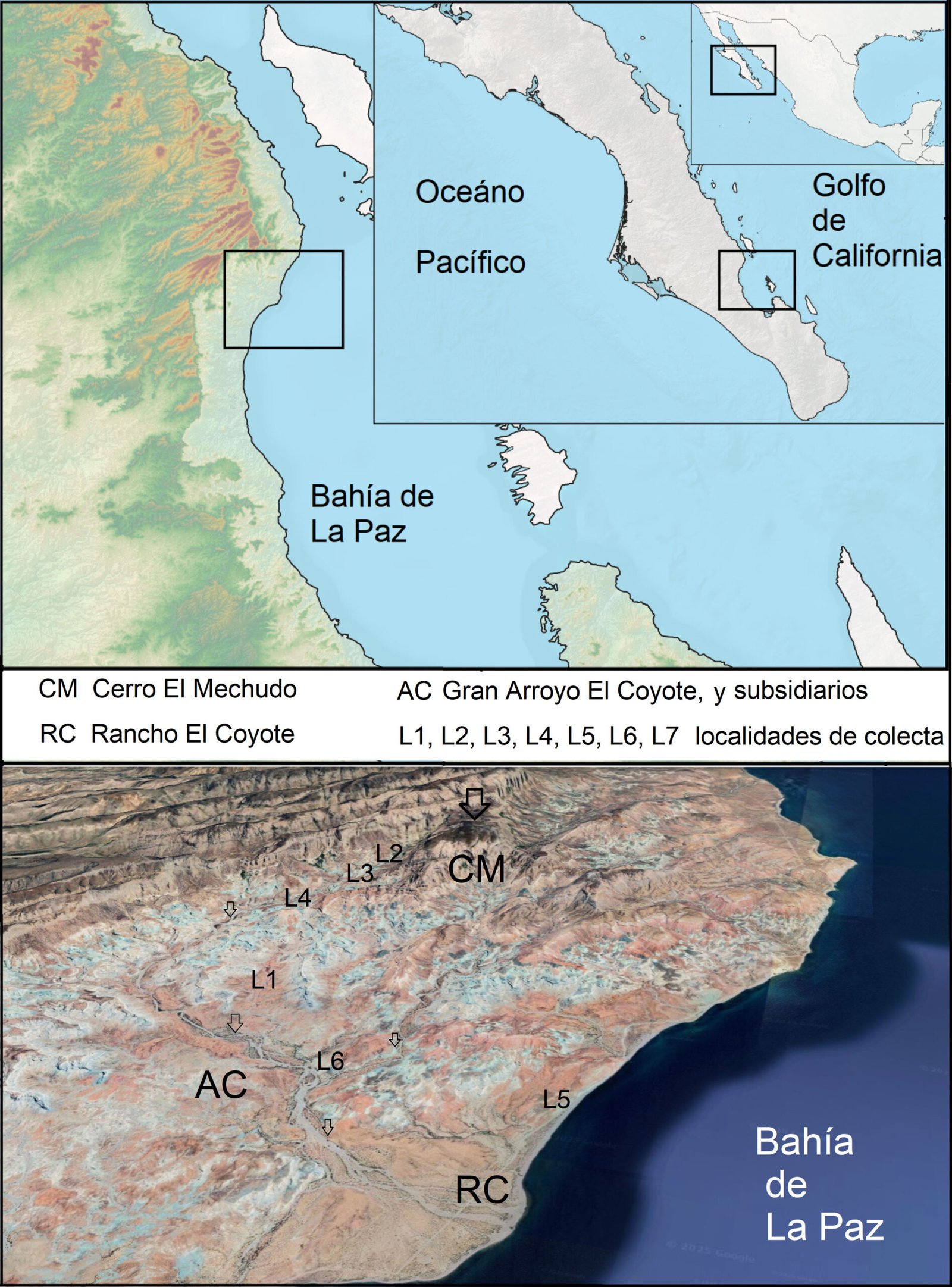
Biogeográficamente, esta zona forma parte de la provincia del Desierto Sonorense (Shreve y Wiggins, 1964); a su vez, se encuentra dentro de la subprovincia Costa Central del Golfo (Rebman et al., 2016), misma que ocupa una larga y estrecha franja de colinas y tierras bajas a lo largo de la costa oriental de la mayor parte de la península, bajo la influencia ambiental, cálida y seca, del golfo de California.
Después de las fuertes lluvias de octubre de 2023, se visitó el arroyo Coyote en diciembre, en búsqueda de nuevas colectas de esas plantas. En la localidad de La Angostura, se encontró la primera población en floración plena. Para conocer la secuencia fenológica, se hizo un segundo reconocimiento en la misma zona en marzo de 2024; para entonces, la mayor parte de las plantas pasaron a la etapa de fructificación, aunque algunas todavía en floración. La figura 1 muestra también la posición geográfica de las colectas y los sitios de observación de las poblaciones, a través del arroyo principal y sus tributarios.
Se realizó un examen meticuloso de los caracteres morfológicos en los ejemplares vivos en estado reproductivo. La morfología de esta novedad se comparó con la de ejemplares de Lippia palmeri, que crecen adjuntos y con otros colectados en la península de Baja California, utilizando los lineamientos diagnósticos expuestos en Shreve y Wiggins (1964); dichas comparaciones se realizaron mediante fotografías expuestas en plataformas informáticas (GBIF, 2024; iNaturalistMX, 2024). Además, se compararon los ejemplares con otras especies de Lippia presentes en Baja California Sur, como las 3 endémicas: L. carterae (Moldenke) G.L. Nesom (1991: 187) [para algunos autores, considerada dentro de L. alba (Mill.) N.E. Br. ex Britton et P. Wilson (1925: 141)], L. formosa Brandegee (1891: 163) y L. fastigiata Brandegee (1889: 196) [anteriormente Burroughsia fastigiata (Brandegee) Moldenke (1940: 412)].
Finalmente, se consultaron los tratamientos taxonómicos disponibles para las especies de Lippia nativas de México, en la Flora de Veracruz (Nash y Nee, 1984) y el centro de México (Rzedowski y Calderón-de Rzedowski, 2002; Calderón-de Rzedowski y Rzedowski, 2005).
Para la descripción morfológica se realizaron mediciones de estructuras vegetativas y reproductivas en material fresco, o bien rehidratado, de los ejemplares herborizados. El examen de las características morfométricas del material colectado se realizó con estereomicroscopios Nikon SMZ25 y Zeiss STEMI DV4 Spot. Además, se tomaron fotografías en campo utilizando cámaras Canon EOS 5DS R y Nikon Coolpix B500. La figura 1 fue elaborada mediante el software libre QGIS 3.28.2 (Qgis Develoment Team, 2024), utilizando un modelo sobre un conjunto de datos cartográficos digitales, con el fin de representar una superficie de elevación topográfica continua a lo largo de la costa norte de la bahía de La Paz. El cálculo del área de ocupación AOO (“area of occupancy”) y de EOO (“extent of occupancy”) de la población bajo estudio, se obtuvo utilizando la herramienta de GeoCAT (Bachman et al., 2011), lo cual finalmente permitió valorar la categoría de riesgo, aplicando los criterios de la lista roja de IUCN (2012).
Descripción
Lippia domingeziorum León-de la Luz sp. nov. (figs. 2, 3)
Diagnosis. Lippia domingeziorum seems to be close to L. palmeri, but it differs in the greater size of the flowers (4 × 4 mm vs. 2 × 3 mm), the greater length of the floral bracts (5-8 mm vs. 3-4 mm), the greater size of the floral peduncle (10-12 mm vs 1-3 mm), and the shorter length of the leaves (10-18 mm vs 10-25 mm), as well because the oil of the glands of the vestiture trichomes is not aromatic.
Herbácea o subarbustiva de hasta 120 cm de altura; ramas delgadas, elongadas, delicadas, 2-3 mm diámetro, cuadrangulares en corte transversal, las más largas algo arqueadas y péndulas, con crecimiento difuso, tallos basales de hasta 12 mm de diámetro, indumento de tallos y follaje puberulento. Lámina foliar gruesa, apenas involutas, principalmente espatuladas a algo cuneadas en contorno, 10-18 mm de largo y 3-5 mm de ancho en el ápice; 6-lóbulos en 3 pares en la mitad superior, cada par de lóbulos simétricos, obtusos, el par basal más grande que los distales que tienden a ser similares en tamaño y forma; indumento denso y cortamente pubescente a tomentoso, con tricomas cinéreos, más denso en la superficie abaxial y también más abundante en gotas de aceite ambarino, pero carentes de aroma; ápice obtuso, margen eroso, base atenuada, decurrente a lo largo de los cortos pecíolos de 3-4 mm de largo; filotaxia decusada, opuesta o ternada; venación foliar pinnada, con una vena central, o algunas veces con 2 venas secundarias originadas desde la base. Inflorescencias axilares en los nodos, cilíndricas o espigadas, algo acrescentes en la fructificación, sobrepasando las hojas adjuntas al termino del desarrollo, (12-)15-17(-20) mm de longitud; las brácteas ovado-lanceoladas, (5-)7(-8) mm de largo, 4(-5) mm de ancho, dispuestas en 4 series verticales a lo largo del eje de la espiguilla, cada serie desarrolla de 5-6 flores funcionales, el par basal de las brácteas connado y sin flores, el resto de las brácteas individualizadas y con una sola flor funcional asociada, su ápice agudo; en cada nodo del tallo se presentan 2 pedúnculos florales opuestos con su respectiva inflorescencia, 10-12 mm de largo, a veces 4, en 2 pares opuestos. Flores delicadas, fácilmente separadas de su receptáculo al tocarlas, sin aroma, sésiles, nacen individualmente de las axilas de las brácteas; cáliz pequeño, 1.5-2 × 0.5 mm, delgado, membranoso, ovoide, 4 lobado, velutinoso; corola hipocrateriforme, de color rosa o fucsia en el limbo, pero blancas internamente en el tubo, el limbo sobresale sobre la bráctea ± 2 mm, cuando expandido, constituido por 2 labios, el superior entero y oblongo, ya extendido, 2-2.5 mm de alto, 4-4.5 mm de ancho, eroso y algo involuto, el labio inferior 3-lobado, cada lóbulo similar en forma y tamaño, ± 2 mm de largo y ancho, el tubo de la corola de 4(-5) mm de longitud, 2-labiado, el labio superior más extendido que el inferior, el indumento de la corola cortamente pubescente en el exterior, con abundantes tricomas glandulares, internamente glabro; estambres 4, todos incluidos en la corola, didínamos, insertos entre el tubo y el limbo, filamentos 0.5-0.8 mm de longitud, anteras ovadas, 0.5-03 mm de longitud, sin apéndices, celdas paralelas; ovario con 2 lóculos, 1-ovulado; estilo 2-3 mm de longitud, estigma oblicuo 0.5-0.6 mm. Fruto esquizocarpico, 2-2.5 mm de longitud, seco, incluido en el cáliz, pericarpo membranoso, dividiéndose en 2 pirenos en la madurez. Semillas obcónicas o turbinadas, escariosa, sin endospermo.

Resumen taxonómico
Tipo. México. Baja California: municipio La Paz, arroyo La Angostura 2, subsidiario al gran arroyo El Coyote, al sur de la sierra El Mechudo, 24°43’33.13” N, -110°43’10.16” O, 48 m, 23 noviembre 2023, Alfonso Medel Narváez 1587 (holotipo HCIB 32361; isotipos: MEXU, RSA, SD).
Paratipos. México. Baja California Sur: Municipio de La Paz; north of La Paz; north of San Juan de la Costa along coastal road, 2.6 miles north of Punta Coyote, 24°43’48.42” N, -110°41’27.63” O, 248, 18 september 1996, J. P. Rebman 3463 (SD 140358, UCR-112690); 1 km al este del Palmillar, base del cerro El Mechudo, 24°46’14.79” N, -110°44’39.27” O, 223 m, 7 noviembre 2001, M. Domínguez León 3049 (HCIB 16776; SD153579); arroyo secundario La Palma, abajo del cerro Mechudo, 24°47’4.93” N, -110°44’21.37” O, 299 m, 18 marzo 2004, J.L. León-de la Luz 10390 (HCIB 20214); Sierra La Giganta, cerro El Mechudo, vertiente sur, arroyo secundario Palmar de las Sabanillas, 24°47’12.98” N, -110°44’21.12” O, 315 m, 13 julio 2015, R. Domínguez Cadena 4336 (HCIB 30023); arroyo El Coyote, 5 km al NNO del campo pesquero El Coyote, 24°44’22.74” N, -110°44’19.17” O, 84 m, 8 marzo 2024, J. L. León-de la Luz 13341 (HCIB 32362).
Distribución y hábitat. Al parecer, este nuevo taxón es un microendemismo confinado en el sur de la Sierra de la Giganta, propio de los arroyos rocoso-arenosos en las estribaciones del sur de la montaña conocida como cerro Cabeza del Mechudo (fig. 1).
La vegetación en el margen del arroyo incluye especies arborecentes, como: Colubrina viridis (M.E. Jones) M.C. Johnst., Fouquieria burragei Rose, Lysiloma candidum Brandegee, Neltuma articulata (S. Watson) Britton et Rose, Parkinsonia microphylla Torr.; especies de herbáceas perennes como: Bahiopsis chenopodina (Greene) E.E. Schill. et Panero, Erythrostemon pannosus (Brandegee) Gagnon et G.P. Lewis, Errazurizia megacarpa (S. Watson) M.C. Johnst., Porophyllum gracile Benth.; algunas trepadoras, Jacquemontia eastwoodiana I.M. Johnst. y Janusia californica Benth.; cactáceas como Cylindropuntia alcahes (F.A.C. Weber) F.M. Knuth. y Pachycereus pringlei (S. Watson) Britton et Rose.
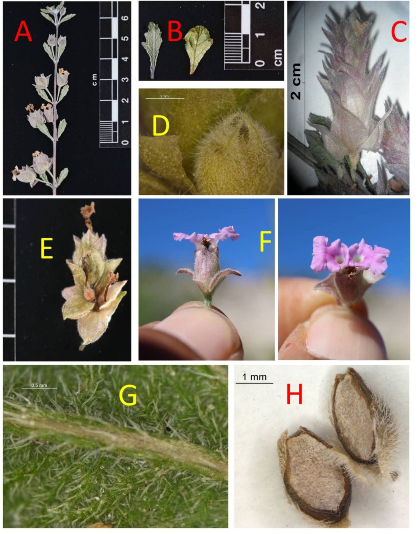
Estatus de conservación. Durante la exploración de campo de 2024, para la búsqueda de plantas sobre el arroyo, se totalizaron 50 ejemplares en una caminata de 1.5 km (elevación de 55 a 90 m). Con ayuda de la herramienta de GeoCAT, se obtiene que la AOO para este nuevo taxón alcanza una superficie de solo 16.7 km2, mientras que el polígono que describe la distribución estimada de la población o EEO, es de 20 km2. Al estimar el tamaño poblacional en AAO, se alcanzarían 1,000 plantas en este mismo sistema de escorrentía pluvial. Aplicando entonces los criterios de la lista roja de IUCN (2012), se determina que la evaluación de esta especie se encuentra en la categoría en peligro crítico (CE), de acuerdo con el criterio B “Distribución geográfica representada como extensión de presencia (B1) y/o área de ocupación (B2)”, específicamente B1 + B2+ a. Adicionalmente, con el número de individuos estimados, se considera a la especie vulnerable (V) dentro del criterio D “Población muy pequeña o restringida”, concretamente
D1 + D2.
Fenología. Las plantas fueron vistas con el follaje la mayor parte del año, incluso los meses de verano. Al incidir suficiente precipitación, las flores aparecen a finales del verano o principios del otoño y aún persisten en los meses de invierno. En la primavera, los frutos alcanzan la madurez, pero las espigas aún portan algunas flores. Los ejemplares visitados en julio estaban ya desprovistos de semillas. Las plantas son palatables para el ganado vacuno y caprino, lo que afecta sensiblemente su desarrollo.
Nombre sugerido y usos. Orégano de los Domínguez, usos no conocidos.
Etimología. El epónimo domingeziorum hace referencia al plural del apellido Domínguez, de los señores Miguel Domínguez y Raymundo Domínguez, 2 valiosos técnicos de campo del herbario HCIB, quienes dedicaron décadas de esfuerzo como colectores y organizadores de la colección, hasta su retiro.
Comentarios taxonómicos
Dentro de la compleja familia Verbenaceae, los altamente diversificados géneros Lantana L. y Lippia L., ambos dentro de la tribu Lantanae, así como otros menos numerosos: Aloysia Ortega ex Juss., Burroughsia Moldenke, Nashia Millsp. y Phyla Lour, no son monofiléticos, como lo han evidenciado Lu-Irving et al. (2021). Tradicionalmente, su taxonomía se ha basado en la morfología de su fruto, pero este es un carácter que no muestra robustez en la reconstrucción filogenética, pues estudios moleculares (O’Leary et al., 2024) proponen que es un rasgo recuperable en los episodios evolutivos inferidos. Mientras se encuentran mejores alternativas para resolver la filogenia de Lantanae, esos autores proponen mantener los nombres de taxones previamente reconocidos en los rangos de tribu, género y sección.
En México, los escasos tratamientos disponibles para Lippia revelan un bajo número de taxones; e.g., la Flora del Bajío (Rzedowski y Calderón-de Rzedowski, 2002) y la Flora de Veracruz (Nash y Nee, 1984) citan 8 taxones cada uno, la flora de Valle de México (Calderón-de Rzedowski y Rzedowski, 2005) solo 1. Para la península de Baja California, la revisión de Rebman et al. (2016) cita 4 taxones válidos (incluido Burroughsia).
Comparando las imágenes disponibles de Lippia palmeri y L. origanoides en la plataforma Naturalista (iNaturalistMX, 2024), es posible respaldar la decisión de que ambas son especies bien diferenciadas y no expresiones geográficas del mismo taxón como alguna vez fue considerado. Entre varios rasgos morfológicos, el primer taxón tiene hojas ovadas con márgenes crenados gruesos, mientras que el segundo tiene hojas oblongas y márgenes dentados. Además, el primero se distribuye en el sector sur del Desierto Sonorense (mitad sur de la península de Baja California y la costa del sur de Sonora) y el segundo se distribuye en México continental y el sur de EUA en variados ambientes (tabla 1).
También, cabe mencionar que alguna vez se propuso al taxón Lippia palmeri var. spicata Rose (1890: 75), sobre la base de ejemplares vistos o recolectados por Edward Palmer en 1890 “cercanos a la población de La Paz, Baja California” (Vasey y Rose, 1890), que sería un lugar ubicado en la misma bahía de La Paz, como la población de L. domingeziorum. Aunque el carácter de ese putativo taxón es una notable “espiga compacta de una pulgada de largo, o más”, hoy en día se conoce que dicho rasgo es relativamente común en ejemplares de L. palmeri que han tenido la oportunidad de continuar su desarrollo vegetativo, pues la espiga es acrecente con la edad de la planta; y si bien la espiga de L. domingeziorum también alcanza estas dimensiones, el carácter que las diferencia es el tamaño notable de la flor y su bráctea adjunta (tabla 1).
Tabla 1
Algunos rasgos de las especies de Lippia en la península de Baja California. Los rasgos están basados en los ejemplares correspondientes depositados en el herbario HCIB, así como en información bibliográfica (Calderón-de Rzedowski y Rzedowski, 2005; Múlgura et al., 1998; Shreve y Wiggins, 1964).
| Carácter | L. domingeziorum | L. carterae (L. alba) | Lippia (Burroughsia) fastigiata | Lippia formosa | L. palmeri |
| Forma de la hoja | Espatulada a cuneada | Ovado-cuneada a oblonga | Cuneada a elíptica | Obovada a cuneada | Diferentes formas; con tendencia a la ovada a cuneado-espatulada |
| Tamaño de la lámina | 10-18 mm longitud, 3-5 mm ancho hacia el ápice | 25-45 mm longitud, 15-30 mm ancho | 4-6 mm longitud, 3-4 mm ancho | 20-30 mm longitud, 8-12 mm ancho al ápice | 10-25 mm longitud, 3-10 mm ancho |
| Ápice de la lámina | Obtuso | Subagudo | Subagudo | Subagudo | Obtuso a subagudo |
| Margen de la lámina | Lobada, con 6 lóbulos simétricos en forma y tamaño | Serrada, a veces crenada en la mitad superior | Crenado en la mitad superior | Gruesamente crenada a dentada en la mitad superior | Subcrenada a gruesamente crenada |
| Inflorescencia | Espigada (madura), 15-25 mm longitud | Capitada a cortamente espigada, 8-12 mm longitud | Capitada, casi esférica, 10-15 mm diámetro | Capitada, casi esférica, 20-25 mm diámetro | Capitada, 4-13 mm longitud |
| Pedúnculo (longitud) | 10-12 mm longitud | 3-5 mm longitud | 4-7 mm longitud | 20-40 mm longitud | 1-3 mm longitud |
| Brácteas (forma y tamaño) | Ovada-lanceolada, 5-8 mm longitud | Ovada, 2-6 mm longitud, foliácea | Ovadas, 1-2 mm de longitud | Cordada, 5-7 mm longitud mayor, membranáceas | Ovada, 3-4 mm longitud |
| Flor (color) | Rosa a fuchsia externamente, blanco en el interior del tubo | Blanco a rosa externamente, amarillo en el interior del tubo | Rosa en los lóbulos del limbo, amarillo en su base y blanco en el interior del tubo | Blanco a rosado | Blanco a amarillo, raramente rosa |
| Flor (tamaño) | Tubo 4 mm longitud, limbo 4 mm ancho | Tubo 2 mm longitud, limbo 3 mm ancho | Tubo 2 mm longitud, limbo 3 mm ancho | Tubo 3 mm longitud, limbo 3-4 mm ancho | Tubo 2 mm longitud, limbo 3 mm ancho |
| Aceite | No aromático | Aromático | Aromático | No aromático | Aromático |
Lippia domingeziorum es morfológicamente semejante a L. palmeri y L. carterae por poseer inflorecencias espigadas, pero se diferencian fácilmente por la morfología foliar. Además, con L. carterae, aunque ambas son microendémicas de sectores de la Sierra de La Giganta, sus poblaciones están separadas por 130 km de distancia; mientras que con L. palmeri ocurre simpátricamente. La figura 4 muestra una lámina comparativa de estas 5 especies.
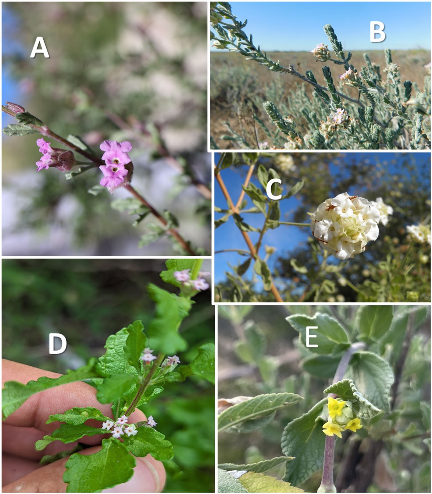
Clave dicotómica, útil para diferenciar entre las especies de Lippia reconocidas para la península de Baja California
1a Androceo con 2 anteras llevando apéndices que se proyectan del conectivo sobre las tecas; cáliz elongado sin brácteas adjuntas
….….….….….….….….….….….….….….….….….….….….….….….….….….…. Lippia (Burroughsia) fastigiata
1b Androceo de 4 estambres sin apéndices; cáliz diminuto, a veces con brácteolas adjuntas
….….….….….….….….….….….….….….….….….….….….….….….….….….…. 2)
2a Brácteas cordadas; inflorescencia capituliforme
….….….….….….….….….….….….….….….….….….….….….….….….….….…. Lippia formosa
2b Brácteas ovado a elípticas; inflorescencia espigada
….….….….….….….….….….….….….….….….….….….….….….….….….….…. (3)
3a Pedúnculo floral largo, de 8-12 mm de longitud
….….….….….….….….….….….….….….….….….….….….….….….….….….…. Lippia domingeziorum
3b Pedúnculo floral corto, de 1-5 mm de longitud
….….….….….….….….….….….….….….….….….….….….….….….….….….….(4)
4a Margen de la hoja crenado a sub-crenado
….….….….….….….….….….….….….….….….….….….….….….….….….….…. Lippia palmeri
4b Margen de la hoja serrado, dentado, o crenado en la mitad superior
….….….….….….….….….….….….….….….….….….….….….….….….….….…. Lippia carterae
Agradecimientos
A Rogelio Amador, propietario del rancho El Coyote por su buena disposición para permitir el trabajo de campo en su predio y su guía para conocer el arroyo Coyote y el paraje de La Angostura durante 2023-2024. Alfonso Medel Narváez generó la figura 1. Danira León Coria realizó el trabajo artístico de la figura 2. También se agradece al editor asociado de Revista Mexicana de Biodiversidad, Arturo Castro Castro, por sus acertados comentarios y sugerencias que mejoraron sustancialmente este manuscrito, así como a Jon P. Rebman del cuerpo de arbitraje y a Jesús González Gallegos consultado sobre la manera correcta de pluralizar el epíteto.
Referencias
Atkins, S. (2004). Verbenaceae. En K. Kubitzki (Ed.), The families and genera of vascular plants 7 (pp. 449–468). Heidelberg, Berlín: Springer. https://id.biodiversity.org.au/reference/apni/47530
Bachman, S., Moat, A. Hill, W., de la Torre, J. y Scott, B. (2011). Supporting Red List threat assessments with GeoCAT: geospatial conservation assessment tool. Zookeys 150,
117–126. https://doi.org/10.3897/zookeys.150.2109
Calderón-de Rzedowski, G. y Rzedowski, J. (2005). Flora fanerogámica del Valle de México, 2ª. Ed. Pátzcuaro, Michoacán: Instituto de Ecología, A.C./ Comisión Nacional para el Conocimiento y Uso de la Biodiversidad.
Cardoso, P. H., O’Leary, N., Olmstead, R. G., Moroni, P. y Thode, V. A. (2021). An update of the Verbenaceae genera and species numbers. Plant Ecology and Evolution, 154, 80–86. https://doi.org/10.5091/plecevo.2021.1821
Conanp (Comisión Nacional de Áreas Naturales Protegidas). (2014). Estudio previo justificativo para el establecimiento del área natural protegida de competencia de la Federación, con la categoría de Reserva de la Biosfera “Sierras La Giganta y Guadalupe”, en el estado de Baja California Sur. Ciudad de México: Semarnat/ Conanp/ Sociedad de Historia Natural Niparajá. Recuperado el 18 agosto 2024 de: https://www.academia.edu/25470101/Reserva_de_la_Biosfera_Sierras_La_Giganta_y_Guadalupe/
García, E. (1998). Climas de México, Cartografía de la clasificación climática de Köppen, modificado por E García. Escala 1:1,000,000. Comisión Nacional para el Conocimiento y Uso de la Biodiversidad, Recuperado el 09 junio 2024 de: http://geoportal.conabio.gob.mx/metadatos/doc/html/clima1mgw.html
GBIF (Global Biodiversity Information Facility). (2024). Lippia alba, Lippia carterae, Lippia formosa, Lippia palmeri, Lippia fastigiata. Recuperado el 27 julio 2024 de: https://www.gbif.org/what-is-gbif
Hausback, B. P. (1984). Cenozoic volcanic and tectonic evolution of Baja California Sur, Mexico (Tesis doctoral). University of California, Berkeley, EUA.
iNaturalistMX. (2024). Lippia alba, Lippia carterae, Lippia formosa, Lippia origanoides, Lippia palmeri, Lippia fastigiata. Recuperado el 30 octubre, 2024 de: https://mexico.inaturalist.org/
IUCN (International Union for Conservation of Nature). (2012). Guidelines for using the IUCN Red List Categories and Criteria, Versión 3.1, 2da ed. Standards and Petitions Committee, IUCN Species Survival Commission. IUCN, Gland. Recuperado el 08 de febrero, 2025, de: https://nc.iucnredlist.org/redlist/content/attachment_files/RedList
Guidelines.pdf
León-de la Luz, J. L. y Domínguez, R. (2006). Hydrophytes of the Sierra de la Giganta oases: composition, structure, and conservation status. Journal of Arid Environment, 67, 553–565. https://doi.org/10.1016/j.jaridenv.2006.03.012
León-de la Luz, J. L., Rebman, J., Domínguez, R. y Domínguez, M. (2008). The vascular flora and floristic relationships of the Sierra de La Giganta in Baja California Sur, Mexico. Revista Mexicana de Biodiversidad, 79, 29–65. https://doi.org/10.22201/ib.20078706e.2008.001.532
León-de la Luz, J. L. y Rebman, J. (2010). A new Ambrosia (Asteraceae) from the Baja California Peninsula, Mexico. Boletín de la Sociedad Botánica de México, 86, 65–70.
Lu-Irving, P., Bedoya, A. M., Salimena, F. R. G., dos Santos-Silva, T. R., Viccini, L. F., Bitencourt, C. et al. (2021). Phylogeny of Lantana, Lippia, and related genera (Lantaneae: Verbenaceae). American Journal of Botany, 108,1354–1373. https://doi.org/10.1002/ajb2.1708
Múlgura, M. E., Martínez, S. y Suyama, A. (1998). Morfología de las inflorescencias de Lippia (Verbenaceae). Darwiniana, 36, 1–12. https://doi.org/10.14522/darwiniana.2014.361-4.316
Nash, D. L. y Nee, M. (1984). Verbenaceae. Flora de Veracruz, 41, 1–51. https://doi.org/10.21829/fv.447.1984.41
O´Leary, N., Lu-Irving, P., Moroni, P., Salimena, F. R. G., dos Santos Silva, T. R., Cardoso, P. H. et al. (2024). Making Lantaneae (Verbenaceae) taxonomy useful: a phylogenetic classification. Taxon, 72, 572–589. https://doi.org/10.1002/tax.12934
QGIS Development Team. (2024). QGIS Geographic Information System. Open Source Geospatial Foundation Project. Recuperado el 01 julio 2024 de: https://www.qgis.osgeo.org
Rebman, J. P., Gibson, J. y Rich, K. (2016). Annotated checklist of the vascular plants of Baja California, Mexico. Proceedings of the San Diego Natural History Museum, 45, 1–352.
Rzedowski, J. y Calderón-de Rzedowski, G. (2002). Familia Verbenaceae. Flora del Bajío y Regiones Adyacentes, 100, 1–145.
Shreve, F. y Wiggins, I. L. (1964). Vegetation and flora of the Sonoran Desert, Vol. 2. Stanford, CA: Stanford University Press.
Thiers, B. (2024). En continua actualización. Index Herbariorum: a global directory of public herbaria and associated staff. New York Botanical Garden’s VirtualHerbarium. Recuperado el 12mayo, 2024 de: http://sweetgum.nybg.org/ih
Vasey, G. y Rose, J. N. (1890). List of plants collected by Dr. Edward Palmer in Lower California and Northwestern Mexico in 1890. Contributions from the United States National Herbarium, 1, 63–78.

A new gall wasp species (Hymenoptera: Cynipidae), Andricus protector Pujade Villar and Cuesta-Porta sp. nova (Hymenoptera: Cynipidae: Cynipini), from Mexico
Una especie nueva de avispa agalladora (Hymenoptera: Cynipidae), Andricus protector Pujade-Villar and Cuesta-Porta sp. nova (Hymenoptera: Cynipidae: Cynipini) de México
Juli Pujade-Villar a, Ricardo Clark-Tapiab, Victor Aguirre-Hidalgo c, George Melikac, Víctor Cuesta-Portaa, *
a Universitat de Barcelona, Facultat de Biologia, Departament de Biologia Evolutiva, Ecologia i Ciències Ambientals, Avda. Diagonal 645, 08028-Barcelona, Spain
b Universidad de la Sierra Juárez, Laboratorio de Estudios Ambientales, Cam. a la Universidad s/n, 68725 Ixtlán de Juárez, Oaxaca, Mexico
c National Food Chain Safety Office, Plant Health Diagnostic National Reference Laboratory, Keleti Károly u. 24, 1024, Budapest, Hungary
*Corresponding author: victorcp93@gmail.com (V. Cuesta-Porta)
Received: 20 January 2025; accepted: 20 August 2025
http://zoobank.org/urn:lsid:zoobank.org:pub:510B361C-ED79-48EB-A484-9100684E3D92
Abstract
A new species of oak gall wasp, Andricus protector Pujade-Villar and Cuesta-Porta sp. nova, known only from its asexual generation that induces deciduous galls on buds of Quercus crassifolia Humb. and Bonpl. (Lobatae section), is described from Mexico. Diagnosis, distribution and biological data of the new species are given. The validity of Andricus species from Mexico is commented. Four species are proposed here to have dubious affiliation: Andricus burnetti (Dailey and Sprenger, 1983), A. marmoreus Kinsey, 1920, A. setifer (Karsch, 1880) and A. strues (Kinsey, 1938).
Keywords: Hymenoptera; Cynipidae; Andricus; New species; Mexico; Quercus crassifolia
Resumen
Se describe una especie nueva de avispa agalladora, Andricus protector Pujade-Villar y Cuesta-Porta sp. nova de México, conocida solo por su generación asexual, que induce agallas deciduas en yemas de Quercus crassifolia Humb. y Bonpl. (sección Lobatae). Se proporcionan la diagnosis, los datos de distribución y biológicos de la nueva especie. Se comenta la validez de las especies de Andricus de México. Cuatro especies tienen afiliación dudosa: Andricus burnetti (Dailey y Sprenger, 1983), A. marmoreus Kinsey, 1920, A. setifer (Karsch, 1880) y A. strues (Kinsey, 1938).
Palabras clave: Hymenoptera; Cynipidae; Andricus; Especie nueva; México; Quercus crassifolia
Introduction
Oak gall wasps (Hymenoptera: Cynipidae: Cynipini) represent the most diverse group within the Cynipidae family, comprising over 1,000 described species in 59 genera (Buffington et al., 2020; Melika, Pujade-Villar et al., 2021; Ronquist et al., 2015; Stone et al., 2002). These wasps induce galls on Fagaceae, primarily on oaks (Quercus L.). In America, north of Mexico, nearly 500 cynipid species have been recorded (Burks, 1979) in association with 90 species of Quercus (Nixon, 2008). In contrast, Europe has approximately 150 described species of cynipids (Melika 2006), despite having only about 30 Quercus species (Uotila, 2011). More specifically, only in the Iberian Peninsula, about 70 cynipid species associated with 10 Quercus species have been documented (Nieves-Aldrey, 2001). Under the same rule-of-thumb, the Mexican oak gall wasp fauna is likely extraordinarily rich, with many species yet to be described, as Mexico is home to 135-161 Quercus species, 86 of which are endemic (Nixon, 1993a, b; Zavala, 1998; Valencia, 2004).
The recorded number of Mexican cynipid species has varied considerably over time. Pujade-Villar et al. (2009) listed 157 cynipid species, with 42 species attributed to the genus Andricus Hartig, 1840. In a subsequent review, Pujade-Villar and Ferrer-Suay (2015) increased the number of Mexican cynipid species to 183, and 43 species of Andricus. More recently, Martínez-Romero et al. (2022) listed 205 species, 30 of which were assigned to Andricus. The genus Andricus is the most diverse, with more than 400 species described worldwide (Melika, Nicholls et al., 2021; Stone et al.,2002), and one of the most taxonomically complex among oak gall wasps.
Since the review by Pujade-Villar et al. (2009), several species previously classified under Andricus have been reassigned to other genera, including Disholandricus Melika, Pujade-Villar and Nicholls, 2021, Dros Kinsey, 1937, Druon Kinsey, 1937, Erythres Kinsey, 1937, Femuros Kinsey, 1937, Feron Kinsey, 1937, Protobalandricus Melika, Nicholls and Stone, 2018, Striatoandricus Pujade-Villar, 2020, and Trichoteras Ashmead, 1897. In Mexico, a total of 31 species of Andricus are listed (Martínez-Romero et al., 2022), later also A. cylindratum (Kinsey, 1937), A. tecturnarum Kinsey, 1920, A. tibialis Kinsey, 1937 (= A. tostum Kinsey, 1937) (= A. uterinus Kinsey, 1937), A. vitreus Kinsey, 1937 (= A. validus Kinsey, 1937) and A. verutus Kinsey, 1937 were transferred to Feron by Cuesta-Porta et al. (2023). Furthermore, since Martínez-Romero et al. (2022), 2 additional Andricus species have been described from Mexico, A. coombesi Pujade-Villar and Pérez-Torres, 2024 and A. mazahua García-Martinón and Pujade-Villar, 2024 (Pujade-Villar et al., 2024, García-Martiñón et al., 2024), bringing the current number of Andricus species in Mexico to 25. Among these, 18 species induce galls on branches, 4 attack buds (rarely leaves or petioles), 1 is found exclusively on leaves, and 1 in acorns. The host of A. aztecus remains unknown, although it is suspected to induce tuberous galls (Martínez-Romero et al.,2022). The new species described here attacks the buds of Q. crassifolia (Lobatae section), producing a distinctive spherical gall with the larval chamber surrounded by longitudinal air chambers divided by thin partitions of spongious tissue.
Materials and methods
Asexual adult gall wasps (ŏ) of the new species described herein were extracted dead from galls on Quercus crassifolia in Oaxaca (Mexico) years after being collected. They were preserved in 100% ethanol in the laboratory by the second author.
The description of the new species follows the current terminology of morphological structures specific for Cynipidae (Liljeblad & Ronquist, 1998; Melika, 2006) and more general sources such as the Hymenoptera Anatomy Ontology Portal (Yoder et al., 2010). Abbreviations for the fore wing venation follow Ronquist and Nordlander (1989); cuticular surface terminology follows that of Harris (1979). Measurements and abbreviations used here include: F1-F11, 1st and subsequent flagellomeres; POL (postocellar distance), the distance between the inner margins of the posterior ocelli; OOL (ocellar-ocular distance), the distance from the outer edge of a posterior ocellus to the inner margin of the compound eye; LOL, the distance between lateral and frontal ocelli. The width of the fore wing radial cell is measured from the margin of the wing to the Rs vein.
The scanning electron microscope (SEM) pictures were taken by the first author at the University of Barcelona (UB) using a field-emission gun environmental scanning electron microscope (FEI Quanta 200 ESEM), with low-resolution imaging without gold-coating the specimens. The photographs of the galls and habitus were taken by the second author with a Canon PowerShot SX510 HS digital camera and a digital camera mounted on Carl Zeiss microscopy III followed by processing with GIMP 2.8 (GNU Image Manipulation Program), respectively.
The type material of the new species is deposited in the University of Barcelona (UB), Catalonia (J. Pujade-Villar coll.).
Andricus protector Pujade-Villar and Cuesta-Porta sp. nova
(Figs. 1-3)
http://zoobank.org/urn:lsid:zoobank.org:act:D806CCCD-2240-4F39-AF38-94D670D404A5
Diagnosis. The new species differs from all Mexican Andricus species by the following combination of characters: mesoscutum transversally rugose; median mesoscutal line present, with smooth bottom; margin of the fore wing shortly ciliated; second metasomal tergum smooth anteriorly, anterolaterally with dense white setae, and a band of punctures in the posterior third; subsequent terga and hypopygium punctuate, without setae. Andricus protector is closely related to Andricus formosalis Weld, 1944 (Fig. 3B), but differs from it by the following characters: antenna and legs brown to black (yellowish in A. formosalis); inner margins of eyes parallel (converging ventrally in A. formosalis); head quadrate and slightly broader than the mesosoma (triangular, narrower than the mesosoma in A. formosalis); F1 1.2 × as long as F2 (only slightly longer in A. formosalis); placodeal sensilla inconspicuous (present in A. formosalis); pronotum completely rugose (with parallel ridges in the posterior margin in A. formosalis); median mesoscutal line long and wide (short and becoming almost inconspicuous in A. formosalis); mesoscutellar foveae quadrate, separated by a carina, not delimited posteriorly (triangular, widely separated and well-delimited posteriorly in A. formosalis); 2nd metasomal tergum occupying most of the metasoma (very short in A. formosalis). Also, the galls of both species are different: with a velvety reddish surface when young and spherical when mature in A. proctector sp. nova, and with a velvety whitish surface when young and ovoid when mature in A. formosalis.
The new species can be morphologically similar to other Andricus inducingtuberous galls in branches. Despite the great divergence in gall morphology between A. protector and the tuberous gallers, Andricus guanajuatensis, A. montezumus, A. peredurus and A. protector have the mesoscutum transversally carinate, whilst the rest of Mexican species that induce tuberous galls have the mesoscutum strongly wrinkled. Andricus protector has a wide band of punctuation in the second metasomal tergum and a medial mesoscutal line (both characters absent in A. guanajuatensis, A. montezumus, and A. peredurus).
Description. Asexual female. Body black (Fig. 3A); mandibles brown, maxillary and labial palpi light brown; antenna brown, scape black; tegula dark brown to black; legs black, tibiae I and II and all tarsomeres brown; metasoma chestnut brown to black; fore wing veins light.
Head (Fig. 1A-D) 1.3 × as broad as high and very slightly broader than mesosoma in frontal view, 2.1 × as broad as long in dorsal view. Gena coriaceous, broadened behind eye, around 1.4 × as broad as transverse diameter of eye; malar space with striae radiating from clypeus and reaching eye; eye 3.1 × as high as length of malar space. Inner margins of eyes parallel. POL 2.0× as long as OOL, OOL 1.3 × as long as diameter of lateral ocellus, 1.3 × as long as LOL, ocelli rounded, all 3 equal in size. Transfacial distance as long as height of eye and 1.35 × as long as height of lower face (distance between antennal rim and ventral margin of clypeus); diameter of antennal torulus 3.3 × as long as distance between them, distance between torulus and eye as long as diameter of torulus. Lower face coriaceous, setose, with some irregular weak striae, with elevated median area coriaceous, with irregular weak striae, without setae. Clypeus quadrate, flat, carinated, ventrally slightly curved, not emarginate and slightly incised medially; with anterior tentorial pit, epistomal sulcus and clypeo-pleurostomal line distinct. Frons, interocellar area and vertex strongly coriaceous, with some weak rugae between ocelli and eye; occiput carinate, with few short setae; postgena punctuate, pubescent; postocciput and postocciput around occipital foramen weakly carinate, glabrous; posterior tentorial pit oval; hypostomal carina emarginate, present at the basis of postgenal sulci, gular sulci present; occipital foramen longer than height of postgenal bridge.
Antenna (Fig. 1E, F) as long as head + mesosoma, with 13 flagellomeres, sometimes with a partial suture towards the middle of F12, rarely F13 fused; pedicel 1.6 × as long as broad, F1 0.8 × as long as length of scape + pedicel and 1.25 × as long as F2, F3 0.8 × as long as F2, F3 as long as F4, F5 as long as F6, F7 slightly shorter than F6 and equal as F8, F9 slightly shorter than F8 and equal as F10, F11 slightly shorter than F10, F12 + 13 shorter than F10 + F11, F12 as long as F11 and slightly longer than F13; placodeal sensilla inconspicuous on F5 – F12, absent on F1 – F4. Antennal formula: 14:11 x 7: 20: 16: 13: 13: 12: 12. 11: 11: 10: 10: 9: 9: 8.
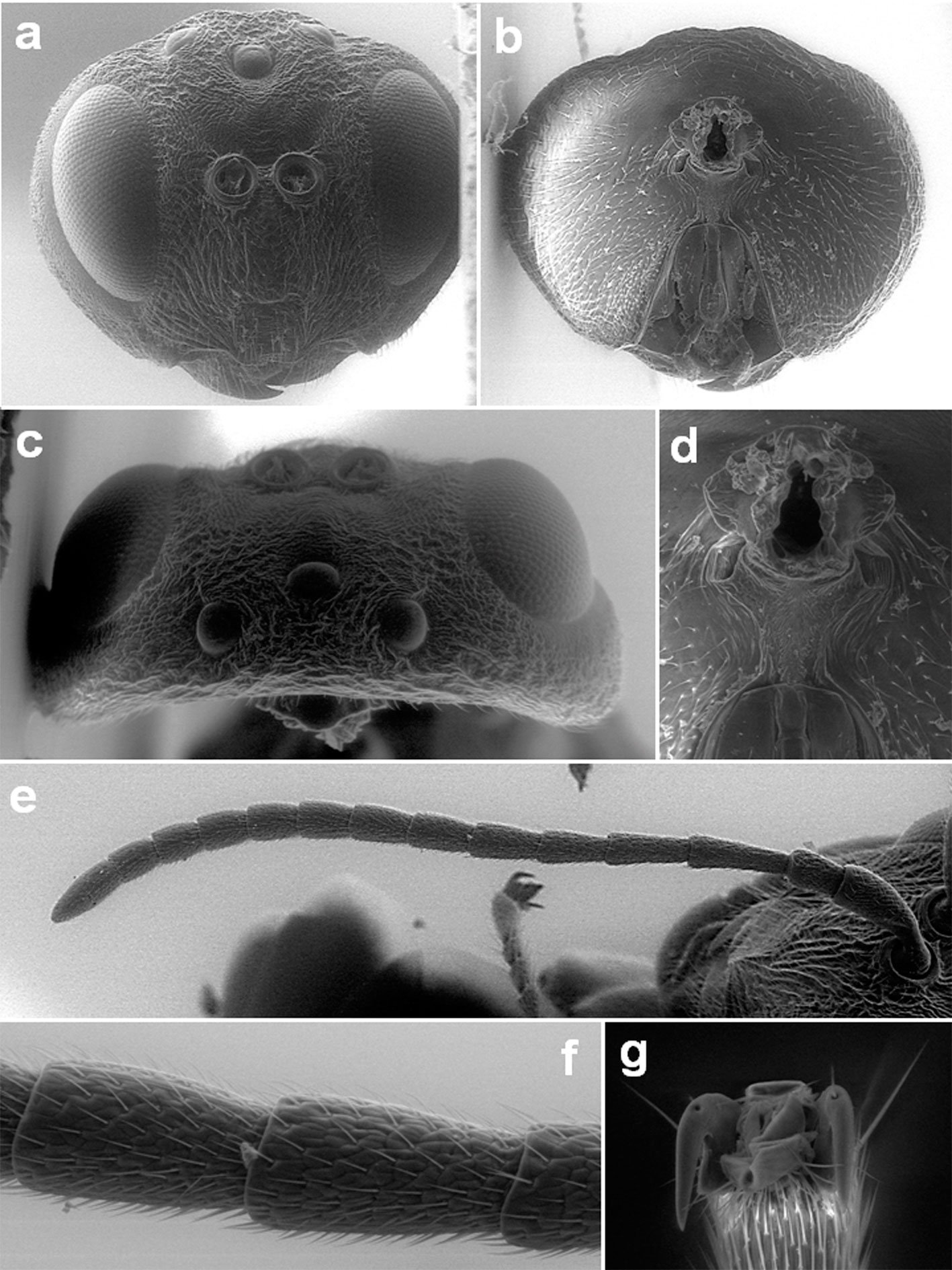
Mesosoma (Fig. 2A-C) slightly longer than high in lateral view. Pronotum rugose with coriaceous interspaces, glabrous, emarginate along lateral and dorsal edges. Propleuron alutaceous with weak irregular rugae and sparse setae. Mesoscutum rugose, with coriaceous interspaces, glabrous, broader than long (width measured across base of tegulae). Notaulus complete; median mesoscutal line present, extends 1/3 of mesoscutum length, with smooth bottom; anterior parallel line impressed, extends to half of mesoscutum length, coriaceous, glabrous; parapsidal line incised and surrounded by coriaceous surface, extends 2/3 of mesoscutum; parascutal carina narrow, coriaceous, reaching notaulus. Transscutal articulation deep, distinct. Mesoscutellum quadrate, shorter than mesoscutum, uniformly rugose, slightly overhanging metanotum; mesoscutellar foveae big, quadrate, with smooth to alutaceous bottom, open basally with some rugae, distinctly divided by a central carina with coriaceous sculpture. Mesopleuron including speculum rugose-carinate, with coriaceous interspaces, sparsely pubescent; mesopleural triangle coriaceous-rugose, with sparse white setae. Metapleural sulcus reaching mesopleuron above half its height, upper part of sulcus inconspicuous; dorsal axillar area rugose, glabrous; lateral axillar area and axillar carina weakly carinated, glabrous; subaxillular bar with parallel sides smooth, glabrous; metanotal trough smooth, setose. Metascutellum sub-rectangle coriaceous, glabrous, ventral impressed area smooth. Lateral propodeal carinae distinct, broad, parallel but basally curved towards the nucha; central propodeal area coriaceous, glabrous, without central longitudinal carina, with some rugae; lateral propodeal area coriaceous rugose, glabrous; nucha with delicate rugae.

![Figure 3. Lateral habitus of a) Andricus protector sp. nova., b) A. formosalis [Picture obtained from Type Search of Smithsonian Entomological Collections, http://n2t.net/ark:/65665/m36fc57b94-797e-4d41-b88c-58776f4ed1d3]](https://rev-mex-biodivers.mx/wp-content/uploads/5448-Fig_3-12cm.jpg)
Fore wing (Fig. 4A) slightly longer than body, hyaline, with the margin shortly ciliate; radial cell open, 3.0 × as long as broad, R1 and Rs not reaching the wing margin; areolet present, large; Rs + M visible in 2/3 of its length, its projection reaching basal vein slightly below half of its height.
Legs with a reticulate sculpture. Tarsal claws with a basal lobe (Fig. 1G).
Metasoma (Fig. 2D, E) shorter than head + mesosoma, longer than high in lateral view, 2nd metasomal tergum smooth anteriorly with dense white setae anterolaterally and a band of punctures in the posterior third; subsequent terga and hypopygium punctuate, without setae; prominent part of the ventral spine of the hypopygium 5.0 × as long as broad in ventral view, with short and sparse white setae, without apical tuft. Body length 3.7-3.8 mm (n = 3).
Gall (Fig. 4B, C). Unilocular, spherical gall located on the axillary buds of Q. crassifolia, in clusters of 2-4, with average size of 11.6 mm (SD ± 0.46 mm, N = 20). Light yellowish red with short pubescent surface when young, turning brown and glabrous when mature. Inside a single larval cell located in the center, surrounded by multiple radiating empty chambers. All chambers are surrounded by spongy tissue. The consistency of the gall is not very hard.
Taxonomic summary
Type material. Holotype: asexual female “MEX, La Resinera, Santa Catarina Ixtepeji (Ixtepec, Oaxaca), Q. crassifolia, (30.vii.2021) extr. 18.v.24”, R. Clark leg. (black label); “holotype Andricus protector Pujade-Villar and Cuesta-Porta n. sp., desig. JP-V 2023” (red label). Paratypes: 3 asexual females with same data as the holotype. Holotype and 3 paratypes are deposited in the collection of JP-V (University of Barcelona, UB), one of them dissected for SEM imaging.
Etymology. Named for the species’ gall model in which the larval chamber is protected (surrounded) by multiple empty chambers.
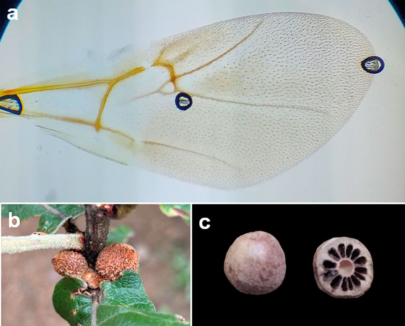
Host plant. Known only from Q. crassifolia (Lobatae section). This oak species is distributed in Mexico (Chiapas, Chihuahua, Guerrero, Guanajuato, Hidalgo, Jalisco, Estado de México, Michoacán, Oaxaca, Puebla, Querétaro, San Luis Potosí, Tlaxcala, Veracruz, and Zacatecas) and Guatemala. Distribution. Mexico (Oaxaca).
Biology. Only the asexual generation is known. The galls appear in mid-June and fall to the ground between August and September, rarely in October. Once in the ground, the galls absorb a lot of soil moisture during the rainy season, which explains why they were very soft when they were collected. This might have affected the development of the adults and prevented them from emerging. The extracted adults were dead, but perfectly preserved.
Discussion
Of the total of 25 Andricus species known from Mexico (Table 1), Andricus burnetti (Dailey & Sprenger, 1983) was described in the genus Trichoteras and transferred to Andricus by Melika and Abrahamson (2002), it is associated with oaks of the Protobalanus section which matches with most Trichoteras species, however the gall differs from the rest of Trichoteras and is more similar to Feron. Andricus marmoreus Kinsey, 1920 has a gall similar to those of Disholcaspis, but the adult has simple tarsal claws and an unusual mesoscutal sculpture for a Mexican species of Disholcaspis. The gall of A. setifer (Karsch, 1880) may correspond to some of the genus Striatoandricus. Lastly, A. strues (Kinsey, 1938) was originally described in the genus Conobius Kinsey, 1938, which was later synonymized under Andricus by Melika and Abrahamson (2002), but unlike what is mentioned in the original description of Conobius, A. strues has the margin of its fore wings ciliated. Concerning Callirhytis quercusbatatoides, Pujade-Villar et al. (2014) mentioned that this species probably belongs to Andricus; later, in Pujade-Villar and Ferrer-Suay (2015), it is considered as an Andricus species but the formal change is not indicated; and finally, in Martínez-Romero et al. (2022) it is definitively named as Andricus quercusbatatoides (Ashmead, 1881).
Among the rest of Andricus species reported from Mexico, the gall morphology and host association is still remarkably diverse (Table 1): one species attacks acorns, 4 induce galls on leaves and/or buds, 3 attack branches without causing globular tuberous galls and 13 induce tuberous galls. The gall of A. aztecus (Cameron, 1888) is unknown, although it may induce tuberous galls.
The alternating life cycle is only known in one of the species (A. quercuslaurinus); the rest remain known by their asexual form except in A. protuberans and A. sphaericus, of which only the sexual generation is known. The Mexican Andricus induce galls in the sections Quercus, Lobatae, Virentes, and Protobalanus (Martínez-Romero et al., 2022; Table 1). The species described here corresponds to an asexual form inducing galls in Lobatae section.
Andricus species with linear elements in the mesoscutum (wrinkles or carinae) are restricted to tuberous gall specie (except A. mazahua). This trait is also present in the species here described, but A. protector does not induce tuberous galls. Among the Mexican Andricus species that produce galls on buds, A. burnetti is associated with Q. palmeri (Protobalanus section), while A. protuberans, A. rochai, and A. strues are associated with species in the Quercus section. Although A. protuberans has also been reported on oaks from the Lobatae section, Cuesta-Porta, Cibrián-Tovar et al. (2022) suggested that these records require further confirmation. Andricus protector has a very peculiar gall containing a set of empty chambers radially surrounding the central larval chamber. The gall of the newly described species is very similar to the gall of A. formosalis known from Arizona also associated with the Lobatae section, but the adults are morphologically different (see Diagnosis and Fig. 3).
Table 1
Andricus species reported in Mexico after this study, indicating the known generation of their lifecycle (Known generation), the plant organ they attack (Plant organ), and the host oak association (Host section). Species marked with an asterisk are considered of unclear affiliation in the Discussion section.
| Species | Authors | Known generation | Plant organ | Host section | |
| Andricus | aztecus | (Cameron, 1888) | Asexual | Unknown | Unknown |
| Andricus | bonanseai | Mayr, 1905 | Asexual | Branch (tuberous) | Lobatae, Quercus |
| Andricus | breviramuli | Pujade-Villar, 2014 | Asexual | Branch (non-tuberous) | Quercus |
| Andricus | burnetti * | (Dailey and Sprenger, 1983) | Asexual | Buds/leaf | Protobalanus |
| Andricus | carrilloi | Pujade-Villar, 2013 | Asexual | Branch (tuberous) | Quercus |
| Andricus | coombesi | Pujade-Villar and Pérez-Torres, 2024 | Asexual | Acorn | Lobatae |
| Andricus | dugesi | Beutenmüller, 1917 | Asexual | Branch (tuberous) | Lobatae, Quercus |
| Andricus | durangensis | Beutenmüller, 1911 | Asexual | Branch (tuberous) | Lobatae |
| Andricus | furnaceus | Kinsey, 1920 | Asexual | Branch (tuberous) | Quercus |
| Andricus | fusiformis | Pujade-Villar, 2014 | Asexual | Branch (non-tuberous) | Lobatae, Quercus |
| Andricus | guanajuatensis | Pujade-Villar, 2013 | Asexual | Branch (tuberous) | Lobatae, Quercus |
| Andricus | marmoreus * | Kinsey, 1920 | Asexual | Branch (non-tuberous) | Quercus |
| Andricus | mazahua | García-Martinón and Pujade-Villar, 2024 | Asexual | Branch (tuberous) | Lobatae |
| Andricus | montezumus | Beutenmüller, 1913 | Asexual | Branch (tuberous) | Quercus |
| Andricus | peredurus | Kinsey, 1920 | Asexual | Branch (tuberous) | Quercus |
| Andricus | protector | Pujade-Villar & Cuesta-Porta, sp. nova. | Asexual | Buds/leaf | Lobatae |
| Andricus | protuberans | Pujade-Villar and Ferrer-Suay, 2015 | Sexual | Buds/leaf | Lobatae |
| Andricus | quercusbatatoides | (Ashmead, 1881) | Asexual | Branch (tuberous) | Virentes |
| Andricus | quercuslaurinus | Melika and Pujade-Villar, 2009 | Sex. and asex. | Branch (non-tuberous) | Lobatae |
| Andricus | rochai | Pujade-Villar, 2018 | Asexual | Buds/leaf | Quercus |
| Andricus | santafe | Pujade-Villar, 2013 | Asexual | Branch (tuberous) | Quercus |
| Andricus | setifer * | (Karsch, 1880) | Asexual | Branch (non-tuberous) | Unknown |
| Andricus | sphaericus | Pujade-Villar, 2016 | Sexual | Buds/leaf | Quercus |
| Andricus | strues * | (Kinsey, 1938) | Asexual | Buds/leaf | Quercus |
| Andricus | tumefaciens | Pujade-Villar and Paretas-Martínez, 2012 | Asexual | Branch (tuberous) | Lobatae, Quercus |
| Andricus | tumeralis | Pujade-Villar, 2009 | Asexual | Branch (tuberous) | Quercus |
Air chambers in galls are hypothesized to act as a defensive mechanism against parasitoids by hindering oviposition or confusing parasitoids simulating larval chambers and (Pujade-Villar et al., 2025; Stone & Cook 1998; Stone et al., 2002). Several independent cynipid lineages have converged into gall morphologies with hollow internal spaces in the parenchyma, such as the galls of Atrusca, Kinseyella, and some Amphibolips in the Nearctic and Trichagalma in Eastern Palearctic, usually exhibit radiating filaments that connect the larval chamber with the outer shell of the gall; or less common cases of free rolling larval chambers like some Disholcaspis or Belizinella (Cuesta-Porta et al.,2020, 2024, 2025; Ide & Koyama, 2023; Pujade-Villar et al., 2010). In the case of A. protector and A. formosalis, galls have hollow longitudinal chambers divided by longitudinal parenchymatous partitions. Despite the gall similarity, the adults of A. protector and A. formosalis exhibit significant differences (see Diagnosis). Further research is needed to determine the phylogenetic relationships between A. protector and the rest of Andricus species. The generic limits of the American Andricus species are still under revision and more data is needed to confirm that the similarities between A. protector and A. formosalis are phylogenetically informative or the result of morphological convergence.
Acknowledgements
We thank Denis Brothers (School of Biological and Conservation Sciences, University of KwaZulu-Natal, Pietermaritzburg, South Africa) for his help with a ZNC question. This research was funded by the project “PID2021-128146NBI00/MCIN/AEI/10.13039/501100011033/” and “FEDER una manera de hacer Europa” from the Ministry of Science and Innovation of Spain and the European Region al Development Fund (ERDF). Also is supported by UNSIJ 2-EA-2203.
References
Buffington, M. L., Forshage, M., Liljeblad, J., Tang, C. T., & van Noort, S. (2020). World Cynipoidea (Hymenoptera): A key to higher-level groups. Insect Systematics and Diversity, 4, 1–69. https://doi.org/10.1093/isd/ixaa003
Burks, B. D. (1979). Superfamily Cynipoidea. In K.V. Krombein, P. D. Hurd Jr., D. R. Smith, & B. D. Burks (Eds.), Catalog of Hymenoptera in America North of Mexico. Vol. 1. (pp. 1045–1107). Symphyta and Apocrita. Washington D.C.: Smithsonian Institution Press.
Cuesta-Porta, V., Equihua-Martínez, A., Estrada-Venegas, E. G., Cibrián-Tovar, D., Barrera-Ruiz, U. M., Ordaz-Silva, S. et al. (2020). Revision of the Amphibolips species of the “nassa” complex from Mexico and Central America (Hymenoptera: Cynipidae). Zootaxa, 4877, 1–50. https://doi.org/10.11646/zootaxa.4877.1.1
Cuesta-Porta, V., Cibrián-Tovar, D., Barrera-Ruiz, U. M., Melika, G., & Pujade-Villar, J. (2022). Andricus protuberans Pujade-Villar and Ferrer-Suay is a sexual form (Hym., Cynipidae, Cynipini). Folia Entomológica Mexicana (nueva serie), 8, e0081004. https://doi.org/10.53749/fem.0081004
Cuesta-Porta, V., Melika, G., Nicholls, J. A., Stone, G. N., & Pujade-Villar, J. (2023). Re-establishment of the Nearctic oak cynipid gall wasp genus Feron Kinsey, 1937 (Hymenoptera: Cynipidae: Cynipini), including the description of six new species. Zootaxa, 5366, 001–174. https://doi.org/10.11646/zootaxa.5366.1.1
Cuesta-Porta, V., Cooke-Mcewen, C., Melika, G., Romero-Rangel, S., Equihua-Martínez, A., Estrada-Venegas, E. G. et al. (2024). Review of the Mexican species of Disholcaspis Dalla Torre & Kieffer with the description of eleven new species. Zootaxa, 5498, 1–100. https://doi.org/10.11646/zootaxa.5498.1.1
Cuesta-Porta, V., Melika, G., Ferrer-Suay, M., Vera-Ortiz, A., & Pujade-Villar, J. (2025). Review of the Nearctic and Neotropical genus Atrusca Kinsey, 1930 (Hymenoptera: Cynipidae, Cynipini). Zootaxa, 5617, 1–195. https://doi.org/10.11646/zootaxa.5617.1.1
García-Martiñón, R. D., Equihua-Martínez, A., Estrada-Venegas, E. G., & Pujade-Villar, J. (2024). Una nueva especie mexicana de Andricus inductora de agallas tumorales en Quercus crassipes. Southwestern Entomologist, 49, 1–11.
Harris, R. (1979). A glossary of surface sculpturing. State of California, Department of Food and Agriculture, Occasional Papers in Entomology, 28, 1–31.
Ide, T., & Koyama, A. (2023). The formation of a rolling larval chamber as the unique structural gall of a new species of cynipid gall wasps. Scientific Reports, 13, 18149. https://doi.org/10.1038/s41598-023-43641-6
Liljeblad, J., & Ronquist, F. (1998). A phylogenetic analysis of higher-level gall wasp relationships (Hymenoptera: Cynipidae). Systematic Entomology, 23, 229–252. https://doi.org/10.1046/j.1365-3113.1998.00053
Martínez-Romero, A., Cuesta-Porta, V., Equihua-Martínez, A., Estrada-Venegas, E. D., Barrera-Ruiz, U. M., Cibrián-Tovar, D. et al. (2022). Aportación al conocimiento de las especies de Cynipini (Hymenoptera: Cynipidae) en los estados mexicanos. Revista Mexicana de Biodiversidad, 93, e933998. https://doi.org/10.22201/ib.20078706e.2022.93.3998
Melika, G. (2006) Gall wasps of Ukraine. Cynipidae. Vestnik Zoologii, 21, 1–300.
Melika, G. & Abrahamson, W. G. (2002). Review of the world genera of oak cynipid wasps (Hymenoptera: Cynipidae: Cynipini). In G. Melika, & C. Thuróczy (Eds.), Parasitic wasps: evolution, systematics, biodiversity and biological control (pp. 150–190). Budapest: Agroinform.
Melika, G., Nicholls, J. A., Abrahamson, W. G., Buss, E. A., & Stone, G. N. (2021). New species of Nearctic oak gall wasps (Hymenoptera: Cynipidae, Cynipini). Zootaxa,
5084, 001–131. https://doi.org/10.11646/zootaxa.5084.1.1
Melika, G., Pujade-Villar, J., Nicholls, J. A., Cuesta-Porta, V., Cooke-McEwen, C., & Stone, G. N. (2021). Three new Nearctic genera of oak cynipid gall wasps (Hymenoptera: Cynipidae: Cynipini): Burnettweldia Pujade-Villar, Melika and Nicholls, Nichollsiella Melika, Pujade-Villar and Stone, Disholandricus Melika, Pujade-Villar and Nicholls; and re-establishment of the genus Paracraspis Weld. Zootaxa, 4993, 1–81. https://doi.org/10.11646/zootaxa.4993.1.1
Nieves-Aldrey, J. L. (2001). Fauna Ibérica, Vol. 16. Hymenoptera: Cynipidae. Madrid: Consejo Superior de Investigaciones Científicas.
Nixon, K. C. (1993a). The genus Quercus in Mexico. In R. Bye, T. P. Ramamoorthy, A. Lot, & J. Fay (Eds.), Biological diversity of Mexico: origins and distribution (pp. 447–458). Nueva York: Oxford University Press.
Nixon, K. C. (1993b). Infrageneric classification of Quercus (Fagaceae) and typification of sectional names. Annales des Sciences Forestières, 50, 25–34. https://doi.org/10.1051/forest:19930701
Nixon, K. C. (2008). Quercus. In Flora of North America @ eFloras. Missouri Botanical Garden, St. Louis, MO y Harvard University Herbaria, Cambridge, MA. Retrieved on September 15, 2020 from: http://www.efloras.org/florataxon.aspx?flora_id=1andtaxon_id=127839
Pujade-Villar, J., Romero-Rangel, S., Chagoyán-García, C., Equihua-Martínez, A., & Estrada-Venegas, E. G. (2010). A new genus of oak gallwasps, Kinseyella Pujade-Villar & Melika, with a description of a new species from Mexico (Hymenoptera: Cynipidae: Cynipini). Zootaxa, 2335, 16–28. https://doi.org/10.11646/zootaxa.2335.1.2
Pujade-Villar, J., Equihua.Martínez, A., & Estrada-Venegas, E. G. (2014). Actualización del conocimiento de los Cynipidae mexicanos que producen agallas en encinos (Hymenoptera: Cynipidae: Cynipini). Entomología Mexicana, 13, 559–564.
Pujade-Villar, J., & Ferrer-Suay (2015). Adjudicació genèrica d’espècies mexicanes d’ubicació dubtosa descrite2s per Kinsey i comentaris sobre la fauna mexicana (Hymenoptera: Cynipidae: Cynipini). Butlletí de la Institució Catalana d’Historia Natural, 79, 7–14.
Pujade-Villar, J., Equihua-Martínez, A., Estrada-Venegas, E. G., & Chagoyán-García, C. (2009). Estado del conocimiento de los Cynipini (Hymenoptera: Cynipidae) en México: perspectivas de estudio. Neotropical Entomology, 38, 809–821. https://doi.org/10.1590/S1519-566X2009000600015
Pujade-Villar, J., Pérez-Torres, B. C., Coombes, A. J., Aragón-García, A., Rodríguez-Acosta, M., López-Olguin, J. F. et al. (2024). Description of the first species of gall wasp (Hym., Cynipidae: Cynipini) on Quercus grahamii (Fagaceae). Zootaxa,5403, 369–376. https://doi.org/10.11646/zootaxa.5403.3.6
Pujade-Villar, J., Melika, G., & Cuesta-Porta, V. (2025). Structure and function of oak gall wasps. In D. C. de Oliveira, & R. M. S. dos Santos Isaias (Eds), Plant galls (pp. 313–347). Cham, Switzerland: Springer.
Ronquist, F., Nieves-Aldrey, J. L., Buffington, M. L., Liu, Z., Liljeblad, J., & Nylander, J. A. A. (2015). Phylogeny, evolution and classification of gall wasps: the plot thickens. Plos One, 10, 1–40. https://doi.org/10.1371/journal.pone.0123301
Ronquist, F., & Nordlander, G. (1989). Skeletal morphology of an archaic cynipoid, Ibalia rufipes (Hymenoptera: Ibaliidae). Entomologica Scandinavica, 33, 1–60
Stone, G. N., & Cook, J. M. (1998). The structure of cynipid oak galls: patterns in the evolution of an extended phenotype. Proceedings of the Royal Society of London. Series B: Biological Sciences, 265,979–988. https://doi.org/10.1098/rspb.1998.0387
Stone, G. N., Schönrogge, K., Atkinson, R. J., Bellido, D., & Pujade-Villar, J. (2002). The population biology of oak gall wasps (Hymenoptera: Cynipidae). Annual Review of Entomology, 47, 633–668. https://doi.org/10.1146/annurev.ento.47.091201.145247
Uotila P. (2011). Quercus. In Euro + Med Plantbase-the information resource for Euro-Mediterranean plant diversity. Retrieved on November 12, 2024 from: http://www.europlusmed.org
Valencia, A. S. (2004). Diversidad del género Quercus (Fagaceae) en México. Boletín de la Sociedad Botánica de México, 75, 33–53. https://doi.org/10.17129/botsci.1692
Yoder, M. J., Mikó, I., Seltmann, K. C., Bertone, M. A., & Deans, A. R. (2010). A gross anatomy ontology for Hymenoptera. Plos One, 5, e15991. https://doi.org/10.1371/journal.pone.0015991
Zavala, F. (1998). Observaciones sobre la distribución de encinos en México. Polibotánica, 8, 47–64.

El grupo pallida del género Phyllophaga (Coleoptera: Melolonthidae) en Oaxaca: nuevos registros y descripción de una especie nueva
The pallida group of Phyllophaga (Coleoptera: Melolonthidae) in Oaxaca: new records and description of a new species
Axel Teodoro Cortes-Dávila a, Salvador Lozano-Trejo a, Andrés Ramírez-Ponce b y Jesús Alberto Cruz-López c, *
a Instituto Tecnológico del Valle de Oaxaca, División de Estudios de Posgrado e Investigación, Ex-hacienda de Nazareno, Agencia de Policía de Nazareno Xoxo, Centro, 71233 Santa Cruz Xoxocotlán, Oaxaca, México
b Instituto de Ecología A.C., Red de Biodiversidad y Sistemática, Carretera Antigua a Coatepec 351, El Haya, 91070 Xalapa, Veracruz, México
c Instituto Nacional de Investigaciones Forestales, Agrícolas y Pecuarias, Campo Experimental Valles Centrales de Oaxaca, Melchor Ocampo Núm. 7, Santo Domingo Barrio Bajo, 68200 Villa de Etla, Oaxaca, México
*Autor para correspondencia: thelyphonidito@gmail.com (J.A. Cruz-López).
Recibido: 24 febrero 2025; aceptado: 23 julio 2025
http://zoobank.org/urn:lsid:zoobank.org:pub:927D7BB0-0BC3-4C5F-8EA1-E2F61BEC7254
Resumen
Uno de los grupos de especies pertenecientes al género Phyllophaga subgénero Phytalus que han recibido especial atención, es el grupo pallida. Actualmente, este grupo está conformado por 12 especies, de las cuales, ninguna se ha reportado para el estado de Oaxaca. En el presente trabajo, se reporta la presencia de este grupo para Oaxaca por primera vez, con base en la revisión del material depositado en el Laboratorio de Entomología Agrícola del Campo Experimental Valles Centrales de Oaxaca – INIFAP. Se aportan nuevos registros para Phyllophaga (Phytalus) dieteriana Deloya et Morón, 1998 y se describe a Phyllophaga (Phytalus) psittacina sp. nov., con base en ejemplares adultos de ambos sexos provenientes de Santa María Tecomavaca, en la Reserva de la Biosfera Tehuacán-Cuicatlán.
Palabras clave: Phytalus; Agave; Selva baja caducifolia; Reserva de la Biosfera Tehuacán-Cuicatlán
Abstract
One of the species groups belonging to the genus Phyllophaga, subgenus Phytalus that has received special attention is the pallida group. Currently, this group includes 12 species, of which none of them has been reported for Oaxaca State. Based on the review of the material deposited in the Laboratorio de Entomología Agrícola of the Campo Experimental Valles Centrales de Oaxaca – INIFAP, we report the presence of this group for the first time for Oaxaca. We provide new records for Phyllophaga (Phytalus) dieteriana Deloya & Morón, 1998, and the description of Phyllophaga (Phytalus) psittacina sp. nov., based on specimens of both sexes from Santa María Tecomavaca, in the Tehuacán-Cuicatlán Biosphere Reserve.
Keywords: Phytalus; Agave; Low deciduous forest; Tehuacán-Cuicatlán Biosphere Reserve
Introducción
El género Phyllophaga Harris, 1827 es uno de los grupos más diversos de la tribu Melolonthini (Coleoptera: Melolonthidae: Melolonthinae), agrupa a un total de 782 especies conocidas en América (Allsopp y Schoolmeesters, 2024). Actualmente, la taxonomía del género está sustentada en caracteres morfológicos externos, principalmente de la morfología de las uñas (Morón, 2015a, b). Sin embargo, estudios sobre la filogenia de Phyllophaga han demostrado que el esquema taxonómico actual debe ser redefinido con base en combinación de caracteres morfológicos que respalden grupos monofiléticos (Rivera-Gasperín y Morón, 2013, 2017a, b). En este sentido, el subgénero Phytalus Erichson, 1847 se reconoce por el ápice de las uñas profundamente hendido o bífido (Morón, 1986). Sin embargo, este subgénero es uno de los que requiere mayor atención taxonómica para el adecuado sustento de sus respectivos grupos. Actualmente, dentro de Phytalus se reconocen 8 grupos de especies, de los cuales solo 3 han sido revisados, teniendo en cuenta las aproximaciones filogenéticas mencionadas anteriormente (Morón, 2006, 2018).
Uno de éstos, el grupo pallida, está conformado por 12 especies distribuidas en los estados de Chihuahua, Colima, Guerrero, Jalisco, Michoacán, Morelos, Nayarit, Puebla, Sinaloa y Sonora, a lo largo de la vertiente del Pacífico, principalmente sobre la provincia biogeográfica Tierras Bajas de Pacífico sensu Morrone et al. (2017). Este grupo puede ser reconocido por tener cuerpo alargado, ovalado, con una longitud de 10 a 15 mm, color pardo rojizo a amarillo, pronoto ligeramente más ancho que la cabeza, antenas formadas por 10 artejos, con los antenómeros tercero al quinto cortos, maza antenal masculina más larga o de igual longitud que el funículo, pronoto y élitros glabros, espolones metatibiales articulados y dentículo inferior de las uñas tarsales de mayor o de similar longitud que el dentículo superior (Morón, 1986, 2006; Romero-López y Morón, 2017). Las especies de este grupo se han recolectado en matorrales xerófilos, bosques espinosos o en bosques tropicales caducifolios, generalmente a no más de 1,000 m snm; son especies poco abundantes, que son atraídas a la luz fluorescente blanca y luz negra (Morón, 2006; Romero-López y Morón, 2017).
De acuerdo con la lista de especies de Phyllophaga reportadas para Oaxaca (Hernández-Cruz et al., 2016), ninguna de las especies del grupo pallida ha sido registrada. Durante la revisión del material depositado en el Laboratorio de Entomología Agrícola del INIFAP – Oaxaca, se hallaron ejemplares de Phyllophaga (Phytalus) dieteriana Deloya et Morón, 1998, que representan el registro más austral para México. Adicionalmente, durante un muestreo de melolóntidos en la Reserva de la Biosfera de Tehuacán-Cuicatlán se recolectaron ejemplares de Phyllophaga (Phytalus) psittacina sp. nov., especie que es descrita a continuación con base en ejemplares de ambos sexos.
Materiales y métodos
Los ejemplares tipo se encuentran depositados en la Colección Entomológica del Instituto de Ecología, A.C. (IEXA), Xalapa, Veracruz y en la Colección Nacional de Insectos (CNIN), Instituto de Biología-UNAM, México. Material adicional se encuentra depositado en la Colección Entomológica del Campo Experimental Valles Centrales de Oaxaca (INIFAP). Los ejemplares de P. (Phytalus) psittacina sp. nov., fueron capturados mediante un muestreo aleatorio realizado durante agosto del 2023 y muestreos semanales realizados de febrero del 2024 a enero del 2025, en una parcela de agave espadín Agave angustifolia Haw. localizada en vegetación de selva baja caducifolia, bosque de cactáceas y matorral xerófilo. Para la captura de los ejemplares se utilizó una trampa de luz blanca led de impacto modificada para colectar escarabajos adultos, la cual se ubicó en el centro de la parcela de cultivo. La fuente de luz fue una lámpara de luz blanca led recargable de 36 W. La trampa utilizada se modificó a partir de la trampa de luz tipo embudo propuesta por Morón y Terrón (1988), cambiando al embudo por una pantalla de mica plástica transparente en forma de cruz, de 40 cm de diámetro por 50 cm de alto. El recipiente colector consistió en un bote circular de plástico con capacidad de 20 L, el cual contenía 10 L de solución de agua y jabón como lo sugiere Aragón-García et al. (2018), con la finalidad de romper la tensión superficial del agua y permitir que los ejemplares se hundan en la solución. La trampa estuvo activa desde las 19:00 hasta las 00:00 hrs. Los ejemplares de P. (Phytalus) dieteriana fueron capturados mediante un esfuerzo comunitario entre un técnico promotor de campo y productores de la comunidad adscritos al programa federal Sembrando Vida del municipio de Tezoatlán de Segura y Luna, en Oaxaca. La recolecta de estos ejemplares consistió en la participación ciudadana como parte de las actividades entre los productores, para que, de manera general, conozcan a los insectos asociados con el cultivo de maíz.
Posterior a la recolecta de los ejemplares, éstos fueron etiquetados y transportados al Laboratorio de Entomología Agrícola del INIFAP – Oaxaca para el subsecuente montaje en alfileres entomológicos de acuerdo con los lineamientos descritos por Márquez-Luna (2005). La extracción y montaje de genitales masculinos siguió el procedimiento descrito por Gutiérrez-Carranza (2023). Para la extracción de las placas genitales femeninas se tomó en cuenta, parcialmente, el protocolo de Gutiérrez-Carranza (2023), con la excepción de que estas estructuras fueron limpiadas a mano del tejido adicional, las placas genitales inferiores se separaron entre sí para poder observar a detalle los márgenes completos y, finalmente, estas estructuras fueron preservadas en un microvial con alcohol junto con la respectiva hembra. Todos los ejemplares (n = 10) fueron disecados.
Para la identificación de los ejemplares recolectados, se utilizaron las claves para el reconocimiento de subgéneros y grupos de especies de Morón (1986), así como la monografía del grupo pallida realizada por Morón (2006), también se revisaron las descripciones originales de las especies del grupo descritas en trabajos diferentes a los mencionados: Morón (1992), Deloya y Morón (1998) y Romero-López y Morón (2017). El criterio para reconocer a esta especie como una nueva perteneciente al grupo pallida, fue con base en la revisión de los trabajos citados, así como la comparación detallada tanto de los genitales masculinos y femeninos.
Para la toma de fotografías, se utilizó una cámara Color CMOS C-Mount Microscope Camera, adaptada a un estereoscopio Jewelry Gem Zoom Stereo Microscope con el programa AmScope v. 3.1. Para corregir los efectos de la iluminación artificial se utilizó el domo de iluminación LED armable para fotografía científica y microscópica recomendado por Kawada y Buffington (2016). Se tomaron fotografías a diferentes profundidades, las cuales posteriormente fueron ensambladas mediante el programa Helicon Focus v. 6.7.1.
La terminología usada para la descripción taxonómica de los adultos fue tomada de Morón (2006), la cual es acorde con el grupo de especies tratadas en el presente trabajo. Para establecer la variación, todos los ejemplares (n = 10) fueron medidos.
Resultados
Phyllophaga (Phytalus) dieteriana Deloya et Morón, 1998
Figs. 1, 8
Resumen taxonómico
Distribución conocida. Esta especie ha sido registrada en Morelos y Puebla, en ecosistemas de bosque tropical caducifolio y matorral crasicaule ubicados entre 940 y 1,600 m snm (Morón, 2006).
Registros nuevos.Diecinueve ♂♂, 4 ♀♀ (INIFAP-Oax), México: Oaxaca: Tezoatlán de Segura y Luna, San Isidro el Naranjo (17°36’21.6” N, 97°47’24” O), 27/junio/2022, Col. C. A. Cruz-López. 2 ♀ (INIFAP-Oax), México: Oaxaca: Tezoatlán de Segura y Luna, Tezoatlán centro (17°38’49.2” N, 97°49’1.2” O), 27/junio/2022, Col. C. A. Cruz-López. 2 ♂♂ (INIFAP-Oax) México: Oaxaca: Tezoatlán de Segura y Luna, Juquila de León (17°22’58.8” N, 97°28’8.4” O), 27/junio/2022, Col. C. A. Cruz-López.
Comentarios taxonómicos
Esta especie es fácilmente reconocible dentro del resto del grupo pallida ya que los machos presentan la espuela metatibial inferior muy recurvada (fig. 1B) y la parte distal de los parámeros con numerosas estrías transversales (fig. 1C).
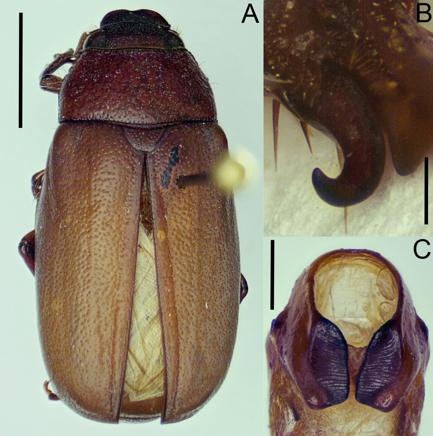
Phyllophaga (Phytalus) psittacina sp. nov.
https://zoobank.org/urn:lsid:zoobank.org:act:F9A4EBC3-67CA-4E61-A7D6-F421DF338E14
Figs. 2-8.
Descripción. Holotipo: (♂, IEXA) con etiqueta roja. Longitud total 19.0 mm, ancho máximo 6.0 mm. Cabeza y pronoto pardo rojizos, élitros, patas y abdomen de color amarillo pajizo brillante (fig. 2A, B). Clípeo semitrapezoidal, con ápice redondeado, ligeramente bilobulado y borde anterior poco elevado; 3.2 veces más ancho que largo; disco clipeal glabro, convexo, con puntos circulares profundos, irregularmente distribuidos (figs. 2A, 3A). Sutura fronto-clipeal bien marcada, ligeramente sinuada. Frente glabra, 2.0 veces más ancha que larga, en sus 2/3 anteriores casi plana con puntos circulares profundos grandes y puntos circulares pequeños irregularmente distribuidos; tercio posterior completamente liso, con muy pequeños puntos someros (figs. 2A, 3A).

Antenas con 10 artejos; segundo artejo más largo y ancho que los artejos III, IV y V, siendo éstos más pequeños, con longitud similar y una proyección anterior semicónica; artejos VI y VII similares en largo y ancho al segundo artejo, y con una proyección anterior semicónica (fig. 3A). Maza antenal más larga que el flagelo (0.9:0.5), formada por 3 lamelas cubiertas con sensilas finas y algunas sedas erectas esparcidas. Anchura dorsal de cada ojo equivalente a 30% de la distancia interocular. Canto ocular corto y estrecho, con 10 sedas (fig. 3A).
Pronoto 1.6 veces más ancho que largo; relación anchura máxima de cabeza-anchura máxima de pronoto de 0.6:1; relación distancia interocular-anchura máxima de pronoto de 0.3:1.
Disco pronotal glabro, con puntos circulares moderadamente profundos, irregularmente esparcidos, más densos hacia la porción media basal. Ángulos anteriores y posteriores obtusos, muy prominentes (figs. 2B, 3A). Bordes laterales levemente redondeados, angulados en su porción central; mitad anterior ligeramente angulada y mitad posterior casi recta; márgenes laterales crenulados en toda su longitud, sobre todo en la mitad anterior (figs. 2B, 3A). Margen basal bien delimitado cerca de ángulos posteriores y ligeramente difuso en parte central (fig. 3A). Escutelo más ancho que largo, con pocos puntos someros dispuestos irregularmente (fig. 3A).
Élitros 3.9 veces más largos que anchos, glabros, con textura punteada de manera irregular pero densa. Reborde de la epipleura muy estrecho, que se desvanece a la altura del propigidio, con sedas cortas muy esparcidas. Callos humerales anteriores prominentes y redondeados; callos posteriores amplios, redondeados, poco prominentes. Alas metatorácicas completamente desarrolladas (fig. 2A, B).

Quinto esternito abdominal poco más largo que el cuarto, con área media central excavada, punteada-rugosa, y algunas sedas erectas cerca del borde posterior, flanqueado por rebordes redondeados transversales (fig. 4A). Placa anal corta, cóncava, con reborde basal transversal y 6 sedas finas cerca de borde posterior.
Protibias más cortas que el tarso respectivo (1:1.3); borde externo con 3 procesos dentiformes, el apical más largo y angosto, ligeramente recurvado, el intermedio grande y ancho, el proximal corto y redondeado (fig. 3A). Espolón protibial ligeramente curvo y aguzado, poco más corto que el segundo protarsómero. Mesotibias con quilla media, setífera transversal oblícuamedia en cara externa bien marcada, precedida por quilla prebasal incompleta. Espolones mesotibiales articulados, rectos, aguzados; externo ligeramente más corto que el interno. Metatibias poco más cortas que tarsos respectivos (1:1.2), con quilla setífera transversal oblicua en tercio distal de la cara externa. Ambos espolones metatibiales articulados; espolón superior más ancho que inferior, poco recurvado, con ápice redondeado, flabelado; espolón inferior recurvado, poco más corto que el superior, con ápice redondeado; espolón superior más largo que primer metatarsómero y el inferior tan largo como éste (fig. 5A). Uñas tarsales profundamente hendidas; dentículo superior de igual longitud que el inferior, ligeramente más estrecho. (fig. 3B).
Cápsula genital masculina con parámeros completamente fusionados en la falobase; extremos apicales punteados y ligeramente divergentes, formando una estructura semicónica, recurvada; ventralmente cada parámero con proyección excavada central que convergen en la parte media, y en la parte basal con una concavidad circular que en conjunto asemejan a un número “8” (fig. 6). Superficie del tectum ampliamente cóncava. Edeago carece de estructura de soporte esclerosada y de ornamentos conspicuos.

Hembra (paratipo IEXA). Muy similar al macho, sin dimorfismo sexual notorio. De tamaño similar al macho, proporciones de las patas similares, abdomen ligeramente más ensanchado y longitud de la maza antenal ligeramente más corta (fig. 2C, D). En cuanto a los espolones metatibiales, el externo tiene casi la misma longitud que el interno, y ambos son apicalmente espatulados (fig. 5B). El carácter sexual más distintivo es la ornamentación del esternito abdominal V, el cual no presenta ningún tipo de rebordes ni ornamentaciones, solo se encuentra cubierto por pocas sedas, esparcidas (fig. 4B). Las placas genitales superiores son alargadas, en forma de lanceta, fusionadas en casi toda su longitud y terminando en un ápice agudo inferior. Por la parte superior, estas placas están ligeramente divergentes, con los bordes engrosados y ligeramente dirigidos hacía la parte ventral, con 6 sedas apicales. Placas inferiores menos esclerosadas, de forma semitriangular y envuelven la mitad inferior de las placas superiores (fig. 7).
Variación. Ambas hembras (n = 2) exhiben tamaños similares, que son ligeramente más grandes que el macho (longitud: 20 mm). Los machos (n = 8) presentan tamaños y proporciones muy similares.
Diagnosis. Esta especie puede ser reconocida de las restantes del grupo pallida por la siguiente combinación de caracteres morfológicos: uñas con dentículo inferior de longitud similar al superior (fig. 3B); maza antenal de similar longitud que el escapo (fig. 3A); quinto esternito abdominal con reborde marcado, en forma de media luna, abarcando más de la mitad del ancho del segmento (fig. 4A); ápices de los parámeros divergentes, con bordes ventrales con concavidad media (fig. 6); placas genitales inferiores fusionadas, en forma de lanceta, con ápices divergentes (fig. 7).

Resumen taxonómico
Material examinado (n = 10): holotipo (♂, IEXA). México: Oaxaca: Santa María Tecomavaca (17°57’46.8” N, 97°01’12” O), 24/agosto/2024, Col. Cortes-Dávila, A. T. 1♂ paratipo (IEXA) con los mismos datos que el holotipo. Un ♂, 2 ♀♀ (IEXA) paratipos con los mismos datos de colecta, pero con fecha del 12/agosto/2023. Un ♂ paratipo (IEXA) con los mismos datos de colecta, pero con fecha del 03/agosto/2024. Dos ♂♂, 1 ♂ y 1 ♂ paratipos (CNIN) con los mismos datos de colecta, pero con las siguientes fechas: 17/agosto/2024, 29/agosto/2024 y 31/agosto/2024, respectivamente.
Etimología. El nombre específico se refiere a la similitud de los parámeros con el pico de la guacamaya verde Ara militaris (Linnaeus, 1766), ave perteneciente al orden Psittaciformes. Adicionalmente, la localidad tipo pertenece al santuario de la guacamaya verde, en la Reserva de la Biosfera Tehuacán-Cuicatlán.
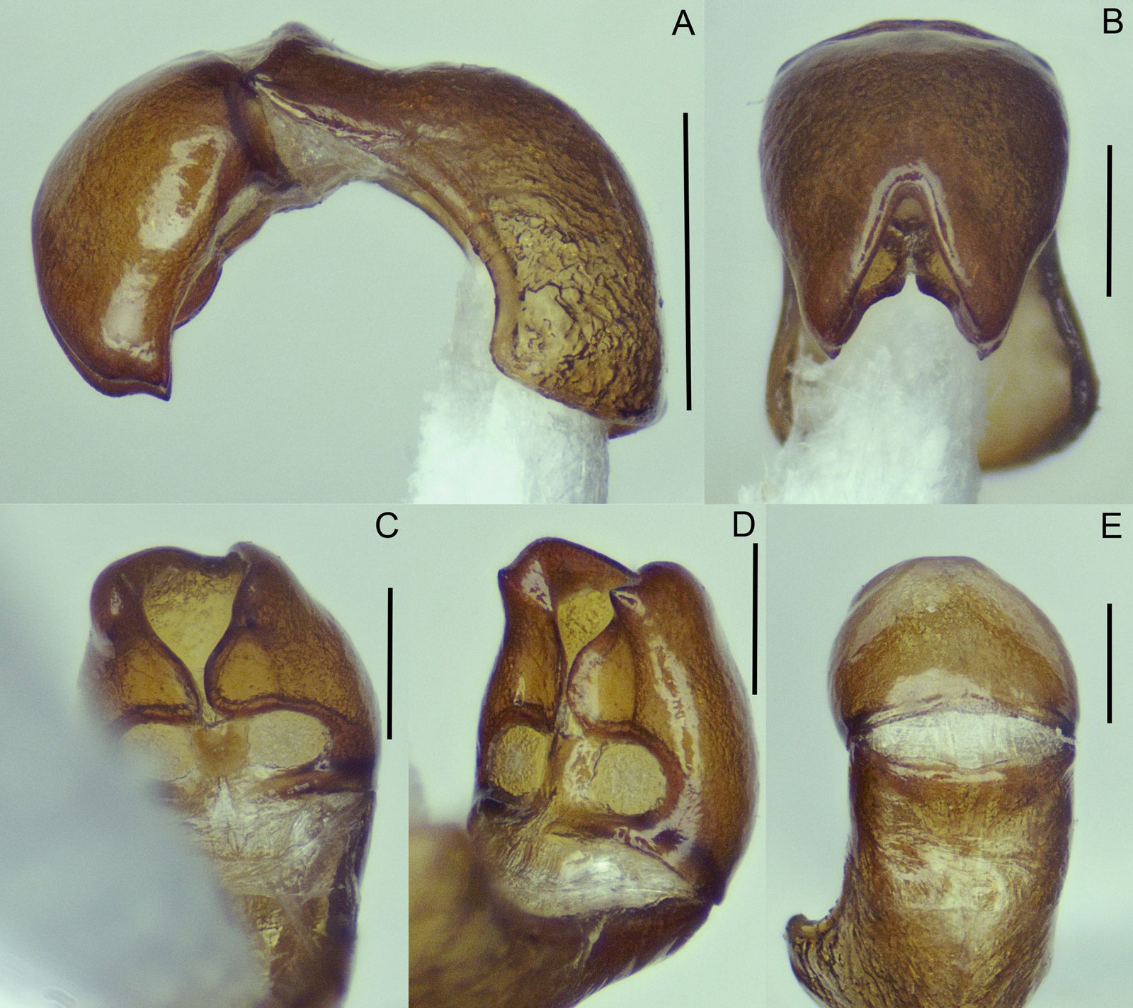
Distribución. Esta especie solo se conoce de la localidad tipo (fig. 8).
Historia natural. Se observó a los escarabajos adultos de P. (Phytalus) psittacina sp. nov. volar y posarse durante la noche en las copas de los árboles de las especies Prosopis laevigata (Humb. et Bonpl. ex Willd) (mezquite blanco), Acacia farnesiana (L.) Willd (huizache) y Citrus aurantifolia (Christm.) Swingle (limón). También se observó que los escarabajos adultos suelen llevar a cabo sus vuelos nupciales en parcelas de cultivo de agave espadín, presumiblemente para alimentarse de las flores o copular en estas plantas. Esta especie convive con los siguientes Rhizotrogina: Phyllophaga (Phyllophaga) lenis (Horn, 1887) y Listrochelus cuicatecus (Morón y Aragón, 1997).
Comentarios taxonómicos
Dentro del grupo pallida, P. (Phytalus) psittacina sp. nov. Es similar a P. (Phytalus) huiteaca Morón, 2006y P. (Phytalus) dieteriana, en la forma del cuerpo, el cual es de tamaño mediano y proporcionalmente esbelto, con una longitud entre 10 a 15 mm, el color pardo rojizo a amarillo, pronoto ligeramente más ancho que la cabeza, antenas formadas por 10 artejos, del tercer al quinto antenómero cortos, maza antenal masculina más larga o de igual longitud que el funículo, pronoto y élitros glabros. En cuanto a la forma de la cápsula genital, P. (Phytalus) psittacina sp. nov. es similar a P. (Phytalus) huiteaca, ya que ambas especies poseen una concavidad media en la parte ventral de los parámeros, sin embargo, en P. (Phytalus) huiteaca los márgenes ventrales que prosiguen de esta concavidad divergen notablemente hasta converger en los ápices, lo cual es inverso en P. (Phytalus) psittacina sp. nov. Desafortunadamente, se desconoce la hembra de P. (Phytalus) huiteaca por lo que las placas genitales no pueden compararse. En cuanto a la morfología genital de la hembra, esta tiene una configuración única entre las especies del grupo, donde las placas genitales inferiores en su parte superior, tienen ligera similitud con aquellas de Phyllophaga (Phytalus) reyesiana, Morón 1992, con los bordes ligeramente divergentes y ornamentados con sedas.

Discusión
De acuerdo con Morón et al. (2014), la abundancia de escarabajos melolóntidos puede categorizarse de acuerdo con el número de ejemplares capturados por métodos convencionales para el grupo. En este sentido, a lo largo del año 2024, se recolectó un total de 7 ejemplares de P. (Phytalus) psittacina sp. nov., todos machos, por lo que esta especie puede considerarse como escasa dentro del rango de clasificación. Las únicas 2 hembras conocidas fueron recolectadas en muestreos aleatorios previos durante el 2023, realizados con la idea de tener una aproximación de la fauna de la zona de estudio. Por otro lado, P. (Phytalus) dieteriana se considera como una especie con abundancia baja (27 ejemplares) en la población reportada como nuevo registro en Oaxaca. Para esta especie, de igual manera la mayor cantidad de ejemplares recolectados fueron machos. La abundancia de los ejemplares de las especies del grupo parece ser baja, capturándose no más de 35 ejemplares por especie (Morón, 2006).
Diversos estudios faunísticos enfocados a la riqueza, diversidad y abundancia de escarabajos melolóntidos en Mesoamérica reportan la presencia de un número variable de especies del género Phyllophaga, así como de otros géneros relacionados de la subtribu Rhizotrogina (e.g., Chlaenobia Blanchard, 1850 y Listrochelus Blanchard, 1850). Los datos de riqueza oscilan entre 4 y 24 especies de Phyllophaga (Aragón-García et al., 2008; Castro-Ramírez et al., 2005; Cuate-Mozo et al., 2016; Delgado et al., 2012; Deloya et al., 1995; Doskocil et al., 2008; Mateos-Escudero et al., 2021; Márquez-Manzano et al., 2023; Ramírez-Ponce et al., 2009). En la localidad tipo de P. (Phytalus) psittacina sp. nov., se está realizando un monitoreo de escarabajos melolóntidos que son atraídos a la luz tipo led blanca. Sorpresivamente, para esta zona, a lo largo de un monitoreo sistemático durante todo el 2024 (además de recolectas aleatorias durante el 2023), solo 3 especies de Rhizotrogina han sido capturadas: P. (Phytalus) psittacina sp. nov. (7 ejemplares), P. (Phyllophaga) lenis (15 ejemplares) y L. cuicatecus (142 ejemplares), consideradas como especies con abundancia moderada y alta, respectivamente. Estos muestreos se realizaron en 3 parcelas diferentes, que abarcan un área aproximada de 2.6 Km2. Morón et al. (2014) mencionan que en ambientes cálido-húmedos y cálido-secos predominan las especies con abundancias moderadas o bajas, como se observa en ambas especies de Phyllophaga. De igual manera, los trabajos enfocados en riqueza y abundancia, indican que existe una menor riqueza de especies en ambientes agrícolas en comparación con ambientes no perturbados, y a su vez, especies con abundancia alta y muy alta en el caso de escarabajos con hábitos alimenticios rizófagos. En la zona de estudio, los muestreos se están realizando en una parcela de agave, por lo que el tipo de ambiente cálido-seco (matorral xerófilo), más la presencia de cultivos agrícolas perennes, pueden ser los factores determinantes para la poca riqueza y abundancia, por lo menos de las especies de Rhizotrogina.

Con respecto a las restantes especies del grupo pallida, todas ellas se distribuyen en ambientes cálido-secos, abarcando matorrales xerófilos, bosques espinosos y bosques tropicales caducifolios, lo que nos indica la preferencia de estas especies por estos ambientes. La mayoría de las especies de este grupo se distribuye a lo largo de la vertiente del Pacífico, abarca casi en su totalidad a la provincia biogeográfica Tierras Bajas del Pacífico, con excepción de Phyllophaga (Phytalus) pallida (Horn, 1885) y Phyllophaga (Phytalus) sonora Saylor, 1939, las cuales se distribuyen entre los límites al norte de las provincias Tierras Bajas del Pacífico y Sonora (sensu Morrone, 2019; Morrone et al., 2017). Cabe resaltar el caso excepcional de P. (Phytalus) dieteriana, que es la única especie que se distribuye en el centro del país, en Morelos y Puebla, en la parte central de la provincia biogeográfica Cuenca del Balsas, incluyendo los nuevos registros reportados en el presente trabajo. Con la adición de P. (Phytalus) psittacina sp. nov., esta especie se distribuye en la provincia biogeográfica Valle de Tehuacán-Cuicatlán (sensu Rzedowski, 1978), la cual corresponde a la provincia más pequeña, de acuerdo con el criterio de Rzedowski. Sin embargo, de acuerdo con la propuesta de Morrone (2019), el área de distribución geográfica de la especie nueva, corresponde a los límites más hacia el centro-sur de la provincia Cuenca del Balsas. También Morrone (2019) indica que esta provincia se encuentra estrechamente relacionada con las Tierras Bajas del Pacífico, lo cual explicaría la distribución geográfica del grupo pallida. Fitogeográficamente, por lo menos la flora de Asteraceae del Valle de Tehuacán-Cuicatlán se relaciona con las de otras regiones áridas y semiáridas de la provincia Cuenca del Balsas y Tierras Bajas del Pacífico (Villaseñor, 1990); así como ambas provincias comparten un gran número de taxones endémicos de la familia Burseraceae (Becerra y Venable, 1999).
Agradecimientos
El primer autor agradece al Consejo Nacional de Humanidades, Ciencias y Tecnologías (Conahcyt), actualmente Secretaría de Ciencia, Humanidades, Tecnología e Innovación (Secihti), por la beca 1320122 y al Instituto Tecnológico del Valle de Oaxaca (ITVO) por su apoyo a la investigación. Este trabajo fue financiado por el Conahcyt, bajo el proyecto número 320715: “Modelo predictivo como estrategia de control de la gallina ciega (Phyllophaga spp.) con base en información climática y del microhábitat en el suelo en sistemas de mono- y policultivos de maíz nativo en Oaxaca”, apoyo otorgado al autor de correspondencia (JACL). Agradecemos el respaldo durante el trabajo de campo a los productores, por facilitar el acceso a sus parcelas donde se realizaron los muestreos. También agradecemos a César Augusto Cruz López, por su apoyo durante la recolecta de melolóntidos en la región de la Mixteca, Oaxaca. De igual manera, agradecemos a los estudiantes que nos apoyaron con la toma de fotografías y las recolectas en campo, especialmente a Eunice Raquel Avendaño Zavaleta (UMAR) y a Marlon Federico Cortes Dávila (UDEA). Finalmente agradecemos a 2 revisores anónimos quienes dieron acertadas sugerencias a la versión previa del manuscrito.
Referencias
Allsop, P. G. y Schoolmeesters, P. (2024). All genera of the world: Subfamilies Prototroginae, Cretoscarabaeinae, Dynamonodinae, Electrorubesopsinae, Phaenomeridinae, Orphninae, Allidiostomatinae, Aclopinae, Lichniinae, Melolonthinae, Oncerinae, Podolasiinae, Sericinae, Sericoidinae (Animalia: Arthropoda: Insecta: Coleoptera: Scarabaeidae). Megataxa, 12, 104–175. https://doi.org/10.11646/megataxa.12.
Aragón-García, A., Nochebuena-Trujillo, C. D., Morón, M. A. y López-Olguín, J. F. (2008). Uso de trampas de luz fluorescente para el manejo de la gallina ciega (Coleoptera: Melolonthidae) en maíz (Zea mays L.) Agrociencia, 42, 217–223.
Aragón-García, A., Pérez-Torres, B., Aragón-Sánchez, M., Cuate-Mozo, V. A., López-Olguín, J. F. y Lugo-García, G. L. (2018). Estrategias agroecológicas para el control de gallina ciega en cultivos agrícolas. En M. B. Nájera R. y Aragón-García, G. (Eds.), Diversidad, ecología y manejo de insectos rizófagos (pp. 135–147). Ciudad de México: Instituto Nacional de Investigaciones Forestales, Agrícolas y Pecuarias/ La Benemérita Universidad Autónoma de Puebla.
Barria, M. D., Clavijo-Bustos, J. y Ramírez-Ponce, A. (2022). A new species of Phyllophaga (s. str.) schizorhina species group (Coleoptera: Scarabaeidae: Melolonthinae: Rhizotrogini) from Panama. Faunitaxys, 10, 1–5. https://doi.org/10.57800/faunitaxys-10(58)
Becerra, X. J. y Venable, L. (1999). Nuclear ribosomal DNA and its implications for evolutionary trends in Mexican Bursera (Burseraceae). American Journal of Botany, 86, 1047–1057. https://doi.org/10.2307/2656622
Castro-Ramírez, A. E., Delfín-González, E. H., Parra-Tabla, V. y Morón, M. A. (2005). Fauna de melolóntidos (Coleoptera: Scarabaeoidea) asociados al maíz (Zea mays L.) en los Altos de Chiapas, México. Folia Entomológica Mexicana, 44, 339–365.
Cuate-Mozo, V. A., Aragón-García, A., Pérez-Torres, B. C., López-Olguín, J. F., Morón, M. A. y Rojas-Martínez, R. I. (2016). Manejo del complejo gallina ciega (Coleoptera: Melolonthidae) asociado al cultivo de amaranto (Amaranthus hypochrondriacus L.) en Puebla, México. Agrociencia, 50, 889–900.
Delgado, L., Mora-Aguilar, E. F. y Escobar-Hernández, F. (2012). Scarabaeoidea (Coleoptera) of the municipality of Xalapa, Veracruz, Mexico: Inventory and analysis. The Coleopterists Bulletin, 66, 319–332. https://dx.doi.org/10.1649/072.066.0405
Doskocil, J. P., Walker, N. R., Bell, G. E., Marek, M., Reinert, J. A. y Royer, T. A. (2008). Species composition and seasonal occurrence of Phyllophaga (Coleoptera: Scarabaeidae) infesting intensely managed bermudagrass in Oklahoma. Journal of Economic Entomology, 101, 1624–1632. https://doi.org/10.1603/0022-0493(2008)101[1624:SCASOO]2.0.CO;2
Deloya, C. y Morón, M. A. (1998). Nuevas especies de Phyllophaga Harris (Coleoptera: Melolonthidae) de Morelos, Puebla y Chiapas, México. Folia Entomológica Mexicana, 104, 109–119.
Deloya, C., Morón, M. A. y Lobo, J. M. (1995). Coleoptera Lamellicornia (Macleay, 1819) del sur del Estado de Morelos, México. Acta Zoológica Mexicana (nueva serie), 65, 1–42. https://doi.org/10.21829/azm.1995.65651653
Gutiérrez-Carranza, I. G. (2023). Protocolo para disección y montaje de luciérnagas (Coleoptera: Lampyridae). Boletín de la Asociación Mexicana de Sistemática de Artrópodos, 7, 2–6.
Hernández-Cruz, J., Morón, M. A., Sánchez-García, J. A., Martínez-Martínez, L., Jarquín-López, R. y Cerqueda-Reyes, H. (2016). Listado de especies del género Phyllophaga Harris, 1827 (Coleoptera: Melolonthidae, Melolonthinae) en el estado de Oaxaca. Entomología Mexicana (nueva serie), 3, 924–929.
Kawada, R. y Buffington, M. L. (2016). A scalable and modular dome illumination system for scientific microphotograph on a budget. Plos One, 11, e0153426. https://doi.org/10.1371/journal.pone.0153426
Mateos-Escudero, M., Guzmán-Vázquez, H. M., Lozano-Trejo, S., Sánchez-García, J. A. y Pérez-León, M. I. (2021). White grub adults associated with maize (Zea mays L.) at Zaachila, Oaxaca, Mexico. Southwestern Entomologist, 46, 709–724. https://doi.org/10.3958/059.046.0312
Márquez-Luna, J. (2005). Técnicas de colecta y preservación de insectos. Boletín Sociedad Entomológica Aragonesa, 37, 385–408.
Márquez-Manzano, J. P., Aragón-García, A., Cuate-Mozo, V. A. y Pérez-Torres, B. C. (2024). Diversidad de gallinas ciegas (Coleoptera: Melolonthidae) asociadas a pastos ornamentales de la Ciudad de Puebla, México. Entomología Mexicana, 11, 1–5.
Morón, M. A. (1986). El género Phyllophaga en México. Morfología, distribución y sistemática supraespecífica (Insecta: Coleoptera). Publicación 20. Ciudad de México: Instituto de Ecología.
Morón, M. A. (1992). Nuevas especies mexicanas del subgénero Chlaenobia de Phyllophaga (Coleoptera: Melolonthidae). Giornale Italiano di Entomologia, 6, 35–51.
Morón, M. A. (2006). Revisión de las especies de Phyllophaga (Phytalus) grupos obsoleta y pallida (Coleoptera: Melolonthidae: Melolonthinae). Folia Entomológica Mexicana, 45 (Suplemento 1), 1–104.
Morón, M. A. (2015a). Revisión del nuevo grupo de especies “guapilana” de Phyllophaga (s. str.) (Coleoptera: Melolonthidae: Melolonthinae). Boletín de la Sociedad Entomológica Aragonesa, 56, 27–38.
Morón, M. A. (2015b). Revisión del nuevo grupo de especies “quetzala” de Phyllophaga (s. str.) (Coleoptera: Melolonthidae: Melolonthinae). Elytron, 27, 3–28.
Morón, M. A. (2018). Revisión del grupo de especies “pruinosa” de Phyllophaga (Phytalus) (Coleoptera: Melolonthidae: Melolonthinae). Dugesiana, 25, 37–59.
Morón, M. A. y Terrón, R. A. (1988). Entomología práctica. Ciudad de México: Instituto de Ecología.
Morrone, J. J. (2019). Regionalización biogeográfica y evolución biótica de México: encrucijada de la biodiversidad del Nuevo Mundo. Revista Mexicana de Biodiversidad, 90, e902980. https://doi.org/10.22201/ib.20078706e.2019.90.2980
Morrone, J. J., Escalante, T. y Rodríguez-Tapia, G. (2017). Mexican biogeographic provinces: map and shapefiles. Zootaxa, 4277, 277–279. https://doi.org/10.11646/zootaxa.
4277.2.8
Morón, M. A., Nogueira, G., Rojas-Gómez, C. V. y Arce-Pérez, R. (2014). Biodiversidad de Melolonthidae (Coleoptera) en México. Revista Mexicana de Biodiversidad, 85 (Supl.), 293–302. https://doi.org/10.7550/rmb.31834
Ramírez-Ponce, A., Allende-Canseco, J. y Morón, M. A. (2009). Fauna de coleópteros lamelicornios de Santiago Xiacui, Sierra Norte, Oaxaca, México. Acta Zoológica Mexicana (nueva serie), 25, 323–343. https://doi.org/10.21829/azm.2009.252640
Rivera-Gasperín, S. L. y Morón, M. A. (2013). Análisis filogenético del subgénero Phyllophaga (Triodonyx) (Coleoptera: Melolonthidae: Melolonthinae). Revista Mexicana de Biodiversidad, 84, 802–817. https://doi.org/10.7550/rmb.34034
Rivera-Gasperín, S. L. y Morón, M. A. (2017a). Phylogenetic relationships within Phyllophaga Harris (sensu lato) (Coleoptera: Melolonthidae, Melolonthinae) with emphasis on Listrochelus Blanchard. Neotropical Entomology, 46, 1–13. https://doi.org/10.1007/s13744-017-0482-6
Rivera-Gasperín, S. L. y Morón, M. A. (2017b). Relaciones filogenéticas de las especies de Chlaenobia con otros miembros de Phyllophaga s. lato (Coleoptera: Melolonthidae: Melolonthinae). Revista Mexicana de Biodiversidad, 88, 592–607. https://doi.org/10.1016/j.rmb.2017.07.011
Romero-López, M. y Morón, M. A. (2017). Dos nuevas especies de Coleoptera Melolonthidae de la Costa Grande de Guerrero, México. Southwestern Entomologist, 42, 889–900. https://doi.org/10.3958/059.042.0327
Rzwedowski, J. (1978). Vegetación de México. Ciudad de México: Editorial Limusa.
Villaseñor, J. L. (1990). The genera of Asteraceae endemic to Mexico and adjacent regions. Aliso, 12, 685–692.

Neoscelis septentrionalis, una especie nueva de Sonora, México (Coleoptera: Scarabaeidae: Cetoniinae)
Neoscelis septentrionalis, a new Mexican species from Sonora, Mexico (Coleoptera: Scarabaeidae: Cetoniinae)
Leonardo Delgado, Eder F. Mora-Aguilar * y Andrés Ramírez-Ponce
Instituto de Ecología, A.C., Red de Biodiversidad y Sistemática, Carretera Antigua a Coatepec Núm. 351, 91070 Xalapa, Veracruz, México
*Autor para correspondencia: eder.mora@inecol.mx (E.F. Mora-Aguilar)
Recibido: 3 marzo 2025; aceptado: 1 agosto 2025
http://zoobank.org/urn:lsid:zoobank.org:pub:C069AF28-A9C4-45C9-9F15-62F2537D6732
Resumen
Se describe una especie nueva mexicana de escarabajo del género Neoscelis Schoch, del estado de Sonora. Se compara a detalle con la especie más afín, N. longiclava Morón y Ratcliffe y se ilustran sus caracteres diagnósticos. Se incluye una clave para las 5 especies del género. Adicionalmente, se presenta el primer registro de N. dohrni (Westwood) para Zacatecas y se añaden datos sobre la variación de machos de N. longiclava.
Palabras clave: Taxonomía; Scarabaeoidea; México; Especie nueva
Abstract
A new Mexican species of the genus Neoscelis Schoch is described from the state of Sonora. The new species is compared in detail with the most similar species N. longiclava Morón y Ratcliffe, and its diagnostic characters are illustrated. A key to the 5 species of the genus is included. Additionally, the first record of N. dohrni (Westwood) for Zacatecas is presented, and new variation data of the males of N. longiclava are added.
Keywords: Taxonomy; Scarabaeoidea; Mexico; New species
Introducción
La tribu Goliathini Latreille, 1829 (Scarabaeidae: Cetoniinae) se distribuye principalmente en África y Asia, donde se conocen ca. 75 géneros y 521 especies de acuerdo con Krajcík (1998, 2012) y Schoolmeister (2024). En América se conocen solo 7 especies de 2 géneros endémicos de México, Ischnoscelis Burmeister, 1842 y Neoscelis Schoch, 1987 (Morón y Ratcliffe, 1989). Las relaciones filogenéticas de los goliatinos americanos no han sido esclarecidas; sin embargo, se ha mantenido la hipótesis que los relaciona con géneros del trópico asiático de la subtribu Rhomborhinina Westwood, 1842 (antes Coryphocerina Burmeister, 1842) (Morón y Ratcliffe, 1989).
Dentro del género Ischnoscelis se conocen 3 especies de Guerrero, Jalisco, México, Morelos y Sinaloa (Bouchard y Curoe, 2012; Curoe, 2013; Hernández-López et al., 2016). Para el género Neoscelis se han descrito 4 especies, N. coracina Mudge y Ratcliffe, 2003 del sur de Jalisco; N. dohrni (Westwood, 1855) de Aguascalientes, Colima, Durango, centro y norte de Jalisco, Nayarit y Sinaloa; N. hexakrotes García-Morales et al., 2019 de Guerrero y N. longiclava Morón y Ratcliffe, 1989 del oeste de Jalisco, descrito con 1 ejemplar macho (García-Morales et al., 2019; Morón y Ratcliffe, 1989, Mudge et al, 2003; Westwood, 1855). Con base en la revisión y comparación de especímenes de las especies del género Neoscelis en colecciones de México y EUA, describimos una especie de Neoscelis de Sonora.
Materiales y métodos
Se siguió la terminología y caracteres morfológicos usados por Morón y Ratcliffe (1989) y Mudge et al. (2003). La nomenclatura actualizada de las plantas siguió lo establecido en Tropicos (2025). Los ejemplares fueron estudiados con un estereomicroscopio Stemi SV6 Zeiss, las fotografías y medidas fueron tomadas con un estereomicroscopio Nikon SMZ25 y cámara DS-Fi2, las imágenes fueron editadas con el programa NIS-Elements software.
Se revisaron 32 ejemplares de especies de Neoscelis de la Colección Entomológica de la California Academy of Sciences (CASC), de la Colección Entomológica del Instituto de Ecología (IEXA) y de las colecciones particulares de Luis Leonardo Delgado Castillo (LLDC), Eder F. Mora-Aguilar (EMAC) y Andrés Ramírez Ponce (ARPC):
Neoscelis coracina Mudge y Raltcliffe (5): México: Jalisco, Ajijic (1 ♂, ARPC); Mazamitla, 1,720 m, 25-26-IX-2005, G. Nogueira col. (1 ♂, EMAC); idem excepto: 1,680 m, 02-X-2005 (2 ♀♀, EMAC); Puerta el Zapatero, 10-2009, fruit trap, Jesus Aguilar leg. (1 ♀ ARPC)
Neoscelis dohrni (Westwood) (10): México: Jalisco, Ixtlahuacán de los Membrillos, sierra El Travesaño, 29-IX-1995, 1,650 m, (4♂♂, IEXA); San Cristóbal de la Barranca, Mesa de los Caballos, 26-VII-2006, 1,671 m, D. Jimeno col. (1 ♂, EMAC); idemexcepto: 23-VII-2006 (1 ♂, EMAC); San Miguel de Hidalgo, 830 m snm, 15-IX-2003, G. Nogueira col (1 ♂, EMAC); Talpa de Allende, Los Sauces, VI-2012, 1,470 m, pino-encino, Fam. Jimeno-Sevilla cols. (1 ♂, EMAC); Tequila, volcán de Tequila, 17-X-2008, 1,380 m (2♂♂, IEXA).
Neoscelis hexakrotes García-Morales et al. (14): México: Guerrero,Acahuizotla, 1,120 m, VII/2017, local collector (3 ♂♂ paratipo, ARPC); Chilpancingo, 1.5 km NE de Acahuizotla, bosque tropical subcaducifolio, 915 m, X/2006, J. Juan López col (1 ♂ holotipo, 1 ♀ paratipo, ARPC); San Roque Mochitlán, 2-X-2018, L. Zacarías L. (1 ♂ paratipo ARPC); idemexcepto: 8-10/IX/2019, (2 ♂♂, 1 ♀ paratipo, ARPC); 18-20/IX/2019, L. Zacarías L. (5 ♂♂ paratipo, ARPC)
Neoscelis longiclava Morón y Ratcliffe (3): México: Jalisco,Estación de Biología Chamela, 7-IX-1989, E. Ramírez. R. A col (3 ♂♂, CAS, IEXA, LLDC).
Utilizamos el concepto filogenético de especie: “Una especie es la agregación más pequeña de poblaciones (sexual) o linajes (asexual) diagnosticables por una combinación única de estados de carácter” (Wheeler y Platnick, 2000). El mapa fue generado utilizando el sitio web SimpleMappr (Shorthouse 2010).
Resultados
Neoscelis septentrionalis sp. nov. Delgado, Mora-Aguilar y Ramírez-Ponce
(figs. 1A-F, 2)
http://zoobank.org/urn:lsid:zoobank.org:act:87061B5E-4746-4671-867C-57FA3873B69D
Diagnosis. Esta especie se diferencia fácilmente de las 4 especies conocidas del género Neoscelis por la combinación de 2 caracteres: maza antenal más larga que los artejos antenales precedentes y protarsómeros con sedas densas en forma de parches en su cara ventral.
Descripción. Holotipo macho: longitud desde ápice del clípeo al ápice de élitros: 19.8 mm, longitud del pronoto 6.6 mm, ancho del pronoto: 7.6 mm, longitud de élitros 12.0 mm, ancho humeral 9.3 mm. Color dorsal y ventral verde obscuro con tonalidades verde metálicas (fig. 1A).
Cabeza con cuerno clipeal corto, aproximadamente el doble de largo que ancho y ampliamente bifurcado casi desde su base. Clípeo rugoso-punteado, moderadamente ensanchado hacia el ápice; con tubérculo preapical a cada lado, divergentes; cóncavo a cada lado de la cresta media longitudinal, sobresaliente ampliamente. Frente irregularmente aplanada a ligeramente cóncava, con puntuación densamente rugosa y setígera, menos marcada hacia el vértice; sedas amarillentas de longitud moderada. Distancia interocular igual a 2.7 veces el ancho interocular de un ojo. Antenas con 10 antenómeros, maza antenal claramente más larga que 7 antenómeros anteriores, longitud del club antenal poco más de un tercio más largo que resto de antenómeros, menos de 3 veces más larga que ancha en vista dorsal (1:0.35) y 3 veces más larga que ancha en vista lateral (fig. 1B-C).
Pronoto semi-hexagonal, lados con reborde marginal, borde basal suavemente sinuado frente al escutelo. Ángulos anteriores, medios y posteriores obtusos y redondeados. Superficie pronotal con puntos setígeros de tamaño moderado y volviéndose rugosos, más grandes y densos hacia los márgenes; sedas pálido-amarillentas erectas, más cortas y finas que las que presenta en la cabeza. Escutelo ligeramente convexo, superficie con escultura similar a la del pronoto. Mesepímero densamente punteado y setígero, sedas finas y de longitud moderada.
Proceso meso-metasternal ligeramente prolongado y redondeado en vista ventral, cara anterior en 80° del plano ventral en vista lateral y con sedas largas y conspicuas. Meso y metasterno con sedas abundantes y largas, mayormente hacia la parte externa, puntuación rugosa transversal.
Protibia larga, esbelta y moderadamente curva, con 2 dientes preapicales pequeños. Protarsómeros ligeramente más largos en longitud que la protibia (incluyendo uñas), con sedas ventrales conspicuas, densas, café amarillentas (carece de los primeros 3 protarsómeros izquierdos (fig. 1A, D). Meso y metatibias esbeltas, ligeramente curvas, con tarsómeros respectivos más largos que su longitud. Meso y metatarsómeros con algunas sedas ventrales hacia el ápice.
Élitros con 3 costillas moderadamente elevadas y lisas, ápices poco marcados, superficiales, intervalos entre ellas con puntos densos de tamaño medio; superficie junto al margen, densa y finamente rugosa, transversalmente a partir del tercio apical.
Esternitos abdominales brillantes, con puntos pequeños y moderadamente densos, con sedas largas y poco densas hacia los lados. Pigidio moderadamente convexo en vista lateral, superficie fina y densamente estrigulada, con sedas pálidas, cortas, erectas y densas.
Genital masculino con parámeros subparalelos en la base, que se ensancha gradualmente hacia el ápice, siendo más ancho en la porción subapical (vista frontal) (fig. 1E); curvados uniformemente, con el ápice doblado ligeramente hacia la porción ventral (vista lateral) (fig. 1F).
Hembra. Desconocida.
Resumen taxonómico
Material tipo. Holotipo ♂, primera etiqueta poco legible: “Est???lla [Estrella] / Sonora, Mex. / X-2-33 [1933] // Coll. Jentry [Gentry] // Van Dyke coll” // “Neoscelis / septentrionalis Delgado et al. 2025 / Holotipo ♂”. El ejemplar se encuentra depositado en la CASC.
Etimología. El nombre de esta especie refiere al Septentrión, el hemisferio norte, ya que esta especie es la que se distribuye más al norte de las especies conocidas de Neoscelis.
Distribución. Tomando en cuenta los datos legibles de la etiqueta, a pesar de su mal estado de conservación, logramos deducir que se hace referencia a la localidad “La Estrella” o “Cañón Estrella”, asociando la fecha de colecta y colector que en ella aparecen. Howard S. Gentry, fue un botánico californiano y colector del holotipo; realizó sus primeras colectas botánicas para su obra “Rio Mayo Plants” (Gentry, 1942) en otoño de 1933. Este trabajo se realizó en el valle del Río Mayo, particularmente entre el río Cedros y el arroyo Guajaray. La localidad La Estrella fue una de las casi 120 localidades enlistadas en su trabajo. Por su parte, Edwin Van Dyke, profesor de entomología de la Universidad de Berkeley, y parte del staff curatorial de la California Academy of Science, donó su colección particular a esta última (Evans y Hogue, 2004).
Esta especie solo se conoce de la región del valle del Río Mayo de Sonora, en el distrito Sinaloense de la provincia de las Tierras Bajas del Pacífico (Morrone, 2017, 2019). En esta región se presenta un mosaico paisajístico conformado por bosque espinoso dominado por Acacia cocliachantha Humb. y Bonpl. ex Willd. y Neltuma velutina (Wooton) Briton y Rose entre 0 y 450 m snm, bosque tropical caducifolio dominado por Lysiloma divaricatum (Jacq.) J.F. Macbr. y Bursera spp. y encinar, entre 300 y 900 m snm y de 900 a 1,100 m snm, respectivamente (Gentry, 1942; Martínez-Yrizar et al., 2010; Rzedowski, 1978). El Cañón Estrella se encuentra alrededor de 500 m de elevación, presenta una interfase entre el matorral y el bosque tropical caducifolio con sabinos (Taxodium mucronatum Ten.) y encinos-pastizal hacia las partes más altas (Gentry, 1942). El hallazgo de esta nueva especie extiende el rango geográfico de esta tribu alrededor del Trópico de Cáncer, en Sonora, México.
Comentarios taxonómicos
Neoscelis septentrionalis sp. nov presenta la mayor similitud con N. longiclava, especialmente por la longitud de la maza antenal (mayor a los artejos precedentes juntos) y la simplicidad de los ornamentos clipeales, así como el pronoto ligeramente convexo (fig. 1A, G). Ambas especies pueden diferenciarse fácilmente por la abundante vestidura de los protarsómeros en la cara ventral de N. septentrionalis sp. nov. (fig. 1D) —muy pocas sedas dispersas en N. longiclava (fig. 1J). Los cuernos clipeales distales y laterales son desarrollados en N. septentrionalis sp. nov (fig. 1A, B), discretos en N. longiclava (fig. 1G, H). La forma del proceso mesometasternal es de alrededor de 80° en vista lateral (45° en N. longiclava) y presenta coloración verde metálica (negra a verde oscuro brillante en N. longiclava [fig. 1G]). La forma de la maza antenal es más ancha en vista lateral (fig. 1C) y la forma de los parámeros ligeramente más angosta en el ápice (fig. 1E) respecto de N. longiclava (fig. 1I, K). Las hembras de ambas especies son desconocidas.
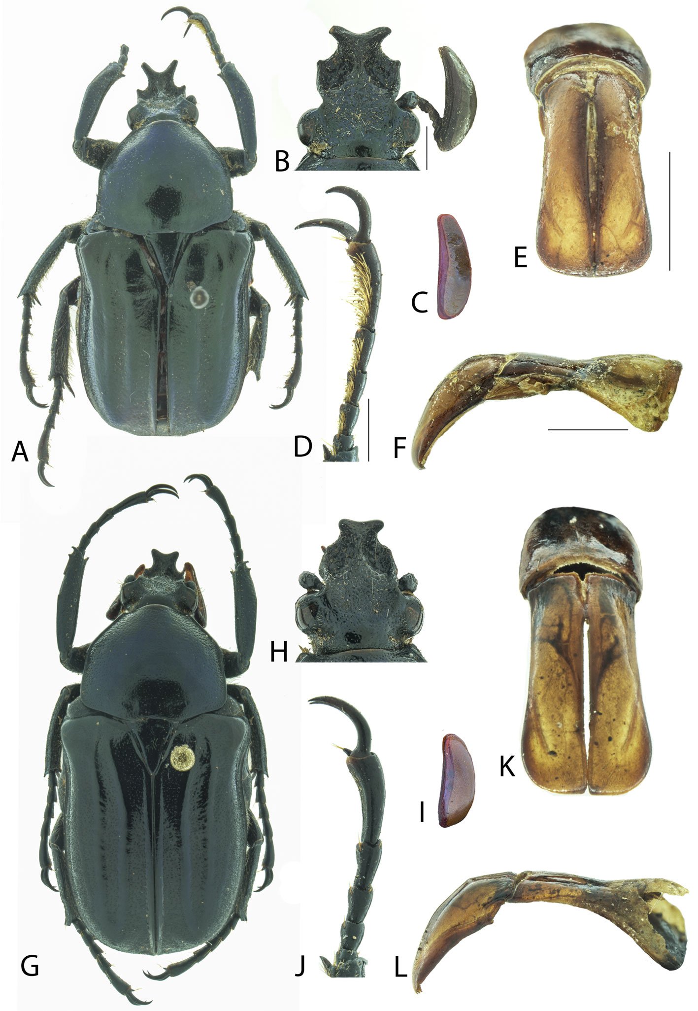
Respecto a las otras especies (N. coracina, N. dohrni y N. hexakrotes), se diferencian fácilmente porque éstas presentan maza antenal pequeña (menor a la longitud combinada de los artejos precedentes), ornamentos clipeales muy desarrollados y elevados, y pronoto fuertemente convexo.
El ejemplar citado por Morón y Ratcliffe (1989) como dudoso (“?”) y que señalan en su mapa de “Sonora: Estuilla” (localidad mal escrita), y reproducido por García-Morales et al. (2019) debe tratarse con toda seguridad de N. septentrionalis.
Neoscelis longiclava Morón y Ratcliffe (fig. 1G-L)
Variación (3♂♂). Longitud total: 18 mm (holotipo) 19.8-22.6 mm, ancho: 9.5 mm (holotipo), 9.7-10.4 mm, 10.2-10.6 mm. Largo de la cabeza: 3.8-4.3 mm, largo del pronoto: 6.3- 6.9 mm; ancho de pronoto: 7.8-8.1 mm, largo élitros: 12.0-13.6 mm.
Coloración dorsal y ventral negra brillante, o verde esmeralda oscuro, metálico, brillante, con cabeza y élitros más oscurecidos (fig. 1G). Maza antenal aproximadamente un tercio más larga que resto de antenómeros, más de 3 veces más larga que ancha en vista dorsal (1:0.29) y 2.5 veces más larga que ancha en vista lateral (fig. 1I). Cuernos clipeales anchos, con ápices redondeados con ancho variable, separación en ángulo obtuso, longitud de los cuernos igual o menor a la longitud de la base (más largos que la base y con ángulo de separación agudo). Base de los cuernos variable pudiendo ser rectangular (más ancha que larga) o subcuadrada (tan ancha como larga). Protarsómeros (incluyendo las uñas) tan largos como la protibia, con sedas pequeñas, poco visibles. Élitros con puntuación fina y densa, ápice de las costillas elitrales fuertemente marcados.
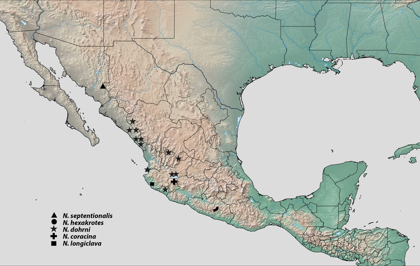
Clave para identificar los machos de las especies de Neoscelis (modificada de García-Morales et al., 2019)
1. Antenas con la maza antenal más larga que los antenómeros precedentes; ornamentos clipeales poco desarrollados; pronoto ligeramente convexo
……………………………………………………………………………… 2
1’. Antenas con la maza antenal más corta que los antenómeros precedentes; ornamentos clipeales notablemente desarrollados; pronoto fuertemente convexo
……………………………………………………………………………… 3
2. Superficie ventral de los protarsómeros con escasas sedas; maza antenal ancha, 2.5 veces más larga que ancha en vista lateral; coloración negra brillante o con ligera tonalidad esmeralda oscuro; oeste de Jalisco
……………………………………………………………………………… N. longiclava Morón y Ratcliffe
2’. Superficie ventral de los protarsómeros con sedas cortas y muy densas; maza antenal estrecha, 3 veces más larga que ancha en vista lateral; coloración verde obscura con tonalidades verde metálicas; Sonora
……………………………………………………………………………… N. septentrionalis sp. nov.
3. Frente convexa; metasterno y abdomen con abundantes sedas hacia la parte externa; Guerrero
……………………………………………………………………………… N. hexakrotes García-Morales, Ramírez-Ponce y Curoe
3’. Frente cóncava; metasterno y abdomen con escasas sedas hacia la parte externa; otros estados pero no en Guerrero
……………………………………………………………………………… 4
4. Carina preocular inclinada anteriormente, sin extenderse hacia la región central; cuerno cefálico profundamente bifurcado, ramas alargadas con tubérculo grande en cara posterior; color dorsal verde metálico, en ocasiones con reflejos cobrizos; de Colima a Durango
……………………………………………………………………………… N. dohrni (Westwood)
4’. Carina preocular extendiéndose hacia la región antero-central; cuerno cefálico moderadamente bifurcado, ramas subtriangulares sin tubérculo en cara posterior; color dorsal negro brillante, a veces con reflejos azul-verde; sur de Jalisco
……………………………………………………………………………… N. coracina Mudge y Ratcliffe
Nuevo registro de distribución de Neoscelis dohrni (Westwood). Se determinaron un macho y una hembra de N. dohrni etiquetados: “Tayahua, Zacatecas, México, 10-XI-1983, 22.0942° N, -102.8695° O, 1,700 m, S. Rosas col.”, ambos depositados en IEXA, que representan el primer registro de la especie para este estado.
Agradecimientos
A la Colección Entomológica de la California Academy of Sciences por el préstamo de ejemplares del género Neoscelis. Expresamos un reconocimiento especial al Dr. Leonardo Delgado (primer autor), quien lamentablemente falleció antes de la publicación de este trabajo, por sus valiosas contribuciones al estudio de los coleópteros de Latinoamérica.
Referencias
Bouchard, D. y Curoe, D. J. (2012). A new species of Ischnoscelis Burmeister, 1842 (Coleoptera, Cetoniinae, Goliatini). Coléoptères, 18, 1–8.
Curoe, D. J. (2013). Description of a third species of Ischnoscelis Burmeister (Coleoptera: Cetoniinae: Goliathini). Besouro, 23, 3–5.
Evans, A. V. y Hogue, J. N. (2004). Introduction to California beetles. Los Angeles, California: University of California Press.
García-Morales, L. J., Ramírez-Ponce, A., Curoe, D. J. y García-Jiménez, J. (2019). A new species of Neoscelis Schoch from Mexico (Coleoptera: Scarabaeidae: Cetoniinae: Goliathini) with new distributional records for the genus. Zootaxa, 4695, 122–130. https://doi.org/10.11646/zootaxa.4695.2.2
Gentry, H. S. (1942). Rio Mayo plants. A study of the flora and vegetation of the valley of the Rio Mayo. Washington, D.C.: Carnegie Institution of Washington. Publication 527.
Hernández-López, N., Delgado, L. y Burgos-Solorio, A. (2016). Description of the female of Ischnoscelis hoepfneri (Gory and Percheron) (Coleoptera: Scarabaeidae: Cetoniinae), notes on the species’ behavior, and a key the species of the genus. The Coleopterists Bulletin, 70, 387–390. https://doi.org/10.1649/0010-065X-70.2.387
Krajcik, M. (1998). Cetoniidae of the World. Catalogue-Part I. República Checa: Typos Studio Most.
Krajcik, M. (2012). Checklist of the world Scarabaeoidea. Anima.X. Supplement 5. República Checa: Plzen.
Martínez-Yrízar, A., Felger, R. S. y Búrquez, A. (2010). Los ecosistemas terrestres: un diverso capital natural. En F. E. Molina-Freaner y T. R. Van Devender (Eds.), Diversidad biológica de Sonora (pp. 129–156). México D.F.: UNAM-Conabio.
Morón, M. A. y Ratcliffe, B. C. (1989). A synopsis of the American Goliatini with description of a new Neoscelis from Mexico. The Coleopterists Bulletin, 43, 339–348.
Morrone, J. J. (2017). Neotropical biogeography: regionalization and evolution. Boca Raton, Florida: CRC Press. https://doi.org/10.1201/b21824
Morrone, J. J. (2019). Regionalización biogeográfica y evolución biótica de México: encrucijada de la biodiversidad del Nuevo Mundo. Revista Mexicana de Biodiversidad, 90, 1–68. https://doi.org/10.22201/ib.20078706e.2019.90.2980
Mudge, A. D., Ratcliffe, B. C., Westcott, R. L. y Noguera, F. A. (2003). A new species of Neoscelis from Jalisco, Mexico (Coleoptera: Scarabaeidae: Cetoniinae). Folia Heyrovskyana, 11, 143–154.
Rzedowski, J. (1978). Vegetación de México. México D. F.: Limusa.
Schoolmeister, P. (2025). World Scarabaeidae database (Version 2025-09-08). En O. Bánki, et al. (Eds.), Catalogue of life. Amsterdam, Países Bajos: Catalogue of Life Foundation. https://doi.org/10.48580/dgt98-38g
Shorthouse, D. P. (2010). SimpleMappr, an online tool to produce publication-quality point maps. Recuperado el 22 de mayo 2025, de: www.simplemappr.net
Tropicos (2025). Tropicos.org. Missouri Botanical Garden. Recuperado el 17 Ene 2025 de https://tropicos.org
Westwood, J. O. (1855). De Coleopteris Goliathidis novi mundo. Linnaea Entomologica, 10, 326–328.
Wheeler Q. D. y Platnick, N. I. (2000). The phylogenetic species concept (sensu Wheeler and Platnick). En Q. D. Wheeler y R. Meier (Eds.), Species concepts and phylogenetic theory: a debate (pp. 55–69). New York: Columbia University Press.

Revision of Hermeniawith descriptions of five new species and a new genus (Polychaeta: Polynoidae)
Revisión de Hermenia con descripciones de cinco nuevas especies y un género nuevo (Polychaeta: Polynoidae)
Patricia Salazar-Silva a, *, Sergio I. Salazar-Vallejo b
a Tecnológico Nacional de México, Instituto Tecnológico de Bahía de Banderas, Crucero a Punta de Mita, 63734 Bahía de Banderas, Nayarit, Mexico
b El Colegio de la Frontera Sur, Unidad Chetumal, Depto. Sistemática y Ecología Acuática, Av. Centenario Km 5.5, 77019 Chetumal, Quintana Roo, Mexico
*Corresponding author: salazarsilva01@yahoo.com (P. Salazar-Silva)
Received: 04 March 2025; accepted: 23 July 2025
http://zoobank.org/urn:lsid:zoobank.org:pub:08AE4922-3010-4327-B8AA-9753DD0AE1D1
Abstract
Hermenia Grube & Örsted (in Grube, 1856) contains 3 described species, with H. verruculosa Grube & Örsted (in Grube, 1856) as its type species and distributed in the Grand Caribbean. H. acantholepis (Grube, 1876) from the Philippines, and H. neoverruculosa Pettibone, 1975 from the Cargados Carajos, Republic of Mauritius. After the revision of type and non-type specimens, differences were observed in body shape, pigmentation pattern, prostomium, size of elytra, dorsal tubercles, and ventral papillae. Type material for the 3 species in the genus was revised, and Hermenia is redefined, its species are redescribed, and 4 species are described: H. chuarae sp. nov. from Indonesia, H. mezianei sp. nov. from Vietnam, H. treadwelli sp. nov. from the Grand Caribbean, and H. wehei sp. nov. from the Arabian Sea. On the other hand, Lepidonotus hermenioides Amoureux, 1974, described from Madagascar, resembles Hermenia species by having papillate integument, but differs by having elytra with long fimbriae. Parahermenia gen. nov. is proposed for including it, and Parahermenia piotrowskiae sp. nov. from Philippines. Identification keys for all species of Hermenia and Parahermenia were included.
Keywords: Caribbean; Lepidonotus; Parahermenia; Scaleworms; Taxonomy
Resumen
Hermenia Grube et Örsted (in Grube, 1856) contiene 3 especies descritas, con H. verruculosa Grube et Örsted (in Grube, 1856) como la especie tipo y distribuida en el Gran Caribe, H. acantholepis (Grube, 1876) de Filipinas y H. neoverruculosa Pettibone, 1975 de Cargados Carajos, República de Mauricio. Después de la revisión del material tipo y de ejemplares no tipo, se observaron diferencias en la forma del cuerpo, en el patrón de pigmentación, prostomium, tamaño de los élitros, tubérculos dorsales y papilas ventrales. El material tipo para las 3 especies fue revisado y Hermenia es redefinida, sus especies son redescritas y se describen 4 nuevas: H. chuarae sp. nov. de Indonesia, H. mezianei sp. nov. de Vietnam, H. treadwelli sp. nov. del Gran Caribe y H. wehei sp. nov. del mar Arábigo. Por otro lado, Lepidonotus hermenioides, descrita de Madagascar, es similar a las especies de Hermenia por tener integumento papilado, pero difiere por tener élitros con fimbria larga. Parahermenia gen. nov. se propone para incluir a ésta y a Parahermenia piotrowskiae sp. nov. de Filipinas. Se proveen claves de identificación para las especies de Hermenia y Parahermenia.
Palabras clave: Caribe; Lepidonotus; Parahermenia; Escamosos; Taxonomía
Introduction
Grube (1850: 36) separated the species of Polynoe Savigny in Lamarck, 1818 after the cover of the dorsum by elytra; in one group he placed all species with elytra large, completely covering dorsum, and in the other, he placed all species with smaller elytra, leaving most of dorsal surface uncovered. In his following paper (Grube, 1851: 120), he added the number of cephalic appendages and separated one species (Polynoe muricata Savigny in Lamarck, 1818) because it has only 4 (no median antenna), and for the other species, he continued using the size of elytra or cover of dorsal surface. In these groups, he used the type of elytra, and their number, sometimes with additional details, to separate similar species, a method that is still used for the whole family.
Kinberg (1856) proposed several new families and genera of scaleworms, and described many species collected during the “Eugenie Expedition”. For the Polynoidae, he proposed 5 genera and diagnosed them, including the elytral cover of the dorsal surface. In Halosydna Kinberg, 1856 the dorsum could be exposed, and in Hermadion Kinberg, 1856, the posterior segments were uncovered.
Hermenia Grube & Örsted in Grube, 1856 was proposed after the finding of an unusual polynoid scale worm because it has a few large elytrae along anterior chaetigers, and minute elytrae in median and posterior segments. The body is robust, and not easily to be broken in parts, as is the case for other polynoids; further, the surface of the body instead of being smooth bears tubercles or papillae, its elytra are fleshy, firmly attached in their elytrophores, and elytra surface has spiny non-sclerotized tubercles and digitiform papillae.
Grube & Örsted in Grube (1856) proposed Hermenia for a species seemingly without palps. Treadwell (1911) noted the palps and corrected the diagnosis for the genus, redescribed H. verruculosa, and regarded Polynoe nodosa Treadwell, 1901 (non P. nodosa Sars, 1861) as a junior synonym. Seidler (1923) redescribed H. verruculosa and redefined the genus to include Lepidonotus acantholepis (Grube, 1876), and redescribed the latter species in a posterior publication (Seidler, 1924).
Hermenia includes H. verruculosa Grube & Örsted in Grube, 1856 from the Caribbean Sea, H. acantholepis (Grube, 1876) from the Philippines, and H. neoverruculosa Pettibone, 1975 from the Seychelles, Indian Ocean. The most recent revision in the genus was carried out by Pettibone (1975) who added the third species: H. neoverruculosa. Pettibone separated the 3 species after the presence of dorsal tubercles or papillae, the number of accessory teeth in neurochaetae, presence of ventral papillae, and number of anterior larger elytrae.
The Caribbean Sea species, H. verruculosa, has been recorded in many localities along the Western Atlantic: New Jersey, Bahamas, Gulf of Mexico, Antilles, and Central to South America, from intertidal down to depths of 220 m (Pettibone, 1975; Salazar-Vallejo, 1996). It has been observed in cracks and interstices of coral rocks (Treadwell, 1911), and it has been reported as living with the brittle starfish Ophiocoma pumilla (now Ophiocomella pumilla [Lütken, 1856] after O’Hara et al., 2019) (Devaney, 1974; Pettibone, 1993). On the other hand, the Indian Ocean species, H. neoverruculosa, is apparently restricted to a few localities, whereas H. acantholepis, described from the Philippines, has been recorded in many localities in the Western Pacific, in coral fragments or on sand (Hanley & Burke, 1991).
During the study of available specimens previously identified as H. verruculosa from different localities along the Grand Caribbean, some were found, indicating the presence of another species. The most relevant differences were the presence of a nuchal lappet (missing in H. verruculosa), the shape of anterior dorsal tubercles, and the pigmentation pattern. First, the anterior margin of chaetiger 2 can be projected anteriorly in a semicircular nuchal lappet, or not projected at all. Second, in most specimens the dorsal tubercles are globular, and in one species they are depressed, being wider than long if seen from above, whereas in a single species they are modified into thin papillae. Third, there are 2 pigmentation patterns; in H. verruculosa there is a rectangular white spot in chaetigers 5 and 6, and in some specimens, there can be paler areas in dorsal surface of parapodia of chaetiger 6, sometimes becoming an inverted T-shaped spot, in the other pattern, the dorsum along first 5-6 chaetigers is completely white, or has an inverted triangular white area. Other species have rather homogeneous pigmentation along the body; further, the dorsal cirrostyle of median segments can be whitish (H. verruculosa), or brownish. These differences were used to separate similar species.
Other morphological features were found to be too variable such as body shape (rectangular vs. fusiform), parapodial size is modified after body contraction, and notochaetae are thin, denticulate capillaries that are usually broken, sometimes from the base, such that their number or presence was regarded as irrelevant for separating similar species.
To standardize these characters, type material of all the described species was examined. Consequently, Hermenia is redefined, H. verruculosa is restricted, and 3 new species are described, 1 from the Grand Caribbean, another one from the Sunda Strait, Indonesia, and a third one from Vietnam. A key to identify all species in Hermenia is also included.
One species, Lepidonotus hermenioides Amoureux, 1974 described from Madagascar, resembles Hermenia species by having papillate integument and neurochaetae with 2-3 additional teeth, but differs from those species by having large elytra in median and posterior segments, each with fimbriate elytra. The finding of another similar species from the Philippines made us propose Parahermenia gen. nov. for including them, and the additional species is described as H. piotrowskiae sp. nov.
Materials and methods
This study was based on the analysis of type material of H. verruculosa, H. acantholepis, and H. neoverruculosa. Further, the study of many specimens previously identified as H. verruculosa from different localities in the Grand Caribbean were examined from the University of Miami, mostly made during their cruises now well-known as University of Miami Deep Sea Expeditions, on board of RVs Gerda and John Elliot Pillsbury (1964-1975), and specimens from the Mexican Caribbean deposited in the Colección de Referencia, ECOSUR, Chetumal (ECOSUR).
Specimens were examined with stereoscopes and with compound microscopes. The length of the specimens was measured from the prostomial anterior margin to the posterior pygidial border, body width was measured in the widest part of the body, including parapodia but excluding chaetae. Body, segmental and parapodial terms follow Pettibone (1975). Segments without elytrae but provided with dorsal cirri are called cirrigers, whereas those having elytrae are called elytrigers.
Drawings were carried out with a camera lucida; some specimens were photographed with a digital camera, and a series of focal successions were compressed with HeliconFocus Ver. 8. Plates were generated with Paint Shop Pro ver. 2021.
To standardize the differences between species the following features were used: a) nuchal lappet over the prostomium, which is an anterior projections from segment 2 (Fig. 5A); b) expansion and anterior projection of the first 2 elytrophores; c) width of the second segment dorsally and in its anterior part, being regarded as narrow if shorter than prostomial width (Fig. 2A), or wide if being as long as, or larger than prostomial width (Fig. 4B); d) parapodial size in comparison to body width, being regarded as long if longer than half body-width, or short if smaller than half body width; e) presence of notochaetae; f) abundance and prominence of dorsal tubercles; g) abundance of ventral papillae; h) size of median and posterior segments elytrae, being regarded as tiny if smaller than dorsal segmental width; i) elytral insertion, being regarded as embedded if not lying on the surface; j) body shape being cylindrical roughly rectangular, fusiform depressed wider anteriorly, swollen wider anteriorly.
Known species are presented in chronological sequence, whereas the newly described taxa will be arranged alphabetically. The material belongs to the following institutions and museums: BMNH: The Natural History Museum, London, England. CAS: California Academy of Sciences, Invertebrate Zoology, San Francisco, California, U.S.A. ECOSUR: Colección de Referencia, El Colegio de la Frontera Sur, Chetumal, Quintana Roo, México. LACM: Natural History Museum of Los Angeles County, Allan Hancock Polychaete collection, Los Angeles, California, U.S.A. MNHN: National Museum of Natural History, Paris, France. MZB: Museum Zoologicum Bogoriense, National Research and Innovation Agency, Cibinong, Indonesia. SMF: Senckenberg Museum, Frankfurt, Germany. UF: Florida Museum of Natural History, University of Florida, Gainesville, Florida, U.S.A. UMML: Museum of Marine Invertebrates, Rosenstiel School of Atmospheric and Marine Sciences, University of Miami, Florida, U.S.A. USNM: National Museum of Natural History, Smithsonian Institution, Maryland, U.S.A. ZMH: Zoologischen Museum und Institut, Hamburg (now Leibniz Institute for the Analysis of Biodiversity Change), Germany. ZMUC: Museum of Zoology, University of Copenhagen, Denmark.
Descriptions
Family Polynoidae Kinberg, 1856
Subfamily Lepidonotinae Willey, 1902
Hermenia Grube & Örsted in Grube, 1856
Hermenia Grube & Örsted in Grube, 1856: 44; Baird, 1865: 200 (diagnosis); Seidler, 1923: 261-262, Fig. 6; Seidler, 1924: 94, Pettibone, 1975. 234 (diagnosis, key); Wehe, 2006: 78 (diagnosis); Salazar-Vallejo & Eibye-Jacobsen, 2012: 1397.
Diagnosis (modificated of Pettibone, 1975). Lepidonotinae with short body; integument tuberculate or papillate, venter smooth or papillate. Body with 26 segments, 12 pairs of elytrae on segments 2, 4, 5, 7, 9, 11, 13, 15, 17, 19, 21, 23. Elytra with globular macrotubercles and microtubercles, few papillae, fimbriae very short; first or first 3 elytra larger than median and posterior ones, most non-overlapping laterally or dorsally. Prostomium bilobed, with 2 pairs of eyes. Tentacular segment with few notochaetae and bulbous facial tubercle. Parapodia sub-biramous, notopodia small, neuropodia large. Notochaetae short, few to absent, slender, finely spinous. Neurochaetae stout, falcate, with 1-2 large accessory teeth. Dorsal cirri with cirrophores cylindrical, cirrostyles short. Ventral cirri short, subulate. Pharynx with 2 pairs of jaws and 11 pairs of marginal papillae. Nephridial papillae short, cylindrical from chaetigers 6-8.
Taxonomic summary
Type species. Hermenia verruculosa Grube & Örsted in Grube, 1856:44, by monotypy.
Distribution. Hermenia includes species from the Western Atlantic, the Indian and Western Pacific Oceans, that have been found mostly in shallow water mixed bottoms.
Remarks
Pettibone (1975) redefined Hermenia, but she did not regard the presence of the nuchal lappet as a distinctive character, although it is present in both H. acantholepis and H. neoverruculosa. The members of this genus are easily distinguished from other species belonging to lepidonotin genera provided with 12 pairs of elytra because, among other features, the reduction of the elytrae in medial and posterior segments, thick neurochaetae with separate accessory teeth, by having integument tuberculate or papillate with transverse lappet, and because the neurochaetae in segments 2 and 3 differ from those present in other segments (see key to genera below).
Hermenia resembles Parahermenia gen. nov. by having a tuberculate or papillate integument, neurochaetae subdistally smooth with tips bi- or tridentate. They differ because in Hermenia the first and last pair of elytra may overlap laterally, with most others being reduced, and by having minute fimbria with abundant macrotubercles; whereas in Parahermenia the elytra overlap laterally and have very long fimbria with few macrotubercles.
Key to Lepidonotinae with 12 pairs of elytra (modified after Fauchald, 1977)
1 With branchial filaments on the elytrophores
……………………………………………………………………………… 2
– Branchial filaments absent
……………………………………………………………………………… 4
2 (1) With pseudelytrae on non-elytrophoral, alternating segments posteriorly
……………………………………………………………………………… Euphionella Monro, 1936
– Pseudelytrae absent
……………………………………………………………………………… 3
3 (2) Neurochaetae coarsely spinose
……………………………………………………………………………… Chaetacanthus Seidler, 1924
– Neurochaetae finely plumose
……………………………………………………………………………… Euphione McIntosh, 1885
4 (1) Notopodia present
……………………………………………………………………………… 5
– Notopodia absent
……………………………………………………………………………… Drieschia Michaelsen, 1892
5 (4) All neurochaetae similar in thickness, without bidentate hooks
……………………………………………………………………………… 6
– With 1 very large bidentate hook in the middle of each neuropodial fascicle
……………………………………………………………………………… Sheila Monro, 1930
6 (5) Neurochaetae subdistally denticulate
……………………………………………………………………………… 7
– Neurochaetae subdistally with 1 or 2 accessory teth
……………………………………………………………………………… 9
7 (6) Notochaetae of 2 kinds, lancet-shaped and tapering and serrated
……………………………………………………………………………… Thormora Baird, 1865
– Notochaetae all of 1 kind, usually slender and serrated
……………………………………………………………………………… 8
8 (7) Pseudelytrae on cirrigerous segments (non-elytrophoral segments)
……………………………………………………………………………… Dilepidonotus Hartman, 1967
– Pseudelytrae absent
……………………………………………………………………………… Lepidonotus Leach, 1816
9 (6) All elytra overlapping laterally, with long fimbriae and a few macrotubercles
……………………………………………………………………………… Parahermenia gen. nov.
– A few anterior elytra overlapping laterally, most elytra small, non-overlapping laterally, fimbria very short, macrotubercles abundant
……………………………………………………………………………… Hermenia Grube & Örsted in Grube, 1856
Hermenia verruculosa Grube & Örsted in Grube, 1856 restricted
(Figs. 1, 2)
Hermenia verruculosa Grube & Örsted in Grube, 1856: 44-45; Treadwell, 1911: 9-11, Figs. 23-26 (partim; Dry Tortugas, Florida, dead coral rock); Seidler, 1923: 261, Fig. 6 (Saint Thomas); Seidler, 1924: 95-96 (Antillas: Barbados and Saint Thomas); Hartman, 1939: 4 (Old providence Island, Colombia, reef in tide pool); Ebbs, 1966: 500, Fig. 4 (Margot Fish Shoal, Florida in coral debris and red coral patch); Pettibone, 1975: 235-238, Figs 1, 2 (synonyms, partim; Gulf of Mexico Florida, off Lousiana, Yucatán, Mexico, low water to 223 m).
Polynoe nodosa Treadwell, 1902: 187, Figs 8, 9 (non Sars, 1861; Fajardo, Puerto rico, Saint Thomas, 20-23 m, coral bottom).
Lepidonotus verruculosus: Horst, 1922: 198 (Caracas bay, Curazao in coral Porites).
Diagnosis. Hermenia with body subrectangular; first pair of elytra bigger, covering prostomium, remaining elytra tiny; dorsal integument with abundant globular tubercles, in segments 4 and 5 forming a pale; segment 2 not projected over prostomium as nuchal lappet; neurochaetae with 1 accessory tooth.
Description. Holotype (ZMUC-1101), complete, body dorsally curved, wider anteriorly, 25 mm long, 6.5 mm wide, 26 segments. Dorsum brownish with transverse pale and dark bands, each segment with dark or pale series of tubercles, densely packed, larger in anterior and posterior segments. Venter smooth or pilose, with abundant thin micropapillae. Segments 5 and 6 with globular pale or colorless papillae arranged in small diffuse pale spots, 1 per segment.
Prostomium bilobed (Fig. 1A), partially retracted into segment 2; facial tubercle round; eyes colorless, 2 pairs, dorsolateral, subdermal, posterior eyes faded color, hidden by peristomium. Median antenna with ceratophore prominent, annulate, inserted frontally, ceratostyle smooth, thin subdistally swollen, with a darker band, tip thin. Lateral antennae with ceratophores cylindrical, ceratostyles thick, smooth, half as long as median antenna, subdistally swollen, tips long. Palps lost.
Tentacular segment indistinct dorsally, without chaetae. Tentaculophores thick, cylindrical. Tentacular cirri unequal to each other, dorsal ones larger, as long as median antenna. Second segment, chaetiger, narrow mid-dorsally with a prominent globular tubercle (Fig. 2A, B), without nuchal lappet. Elytrophores not expanded, nor extended anteriorly (Fig. 1A).
First pair of elytra largest, colorless (Fig. 1B), completely cover prostomium; elytral surface with abundant macrotubercles and cylindrical papillae; macrotubercles wart-like, semispherical, spinulose, larger towards margin, concentrated posteriorly; papillae thick, shorter along elytral margin (Fig. 1C, D), slightly swollen distally (Fig. 1E); other elytra circular, of similar size, strongly adhered in the back, elytral surface with 4 large semispherical macrotubercles, spinulose, and scattered cylindrical papillae, elytral margins with abundant thick, digitate papillae (Fig. 1F).
Parapodia short, as long as half body width; dorsally with traverse arrays of globular tubercles along notopodium, remaining surface with arrays of papillae; ventrally with transverse pleats and scattered tiny papillae (Fig. 1G). Notopodia reduced, acicular lobe small, covered by a small papilla, without notochaetae. Neuropodia slantingly truncated, dorsally furrowed, prechaetal lobe longer than postchaetal one, distally with some papillae.
Cirrigerous segments with cylindrical, thick, short cirrophores, cirrostyles smooth, short, with some filiform papillae, not reaching neurochaetal tips. Ventral cirri with cirrophores thick, very short, cirrostyles thick, short, tapered. Nephridial papillae from segment 7, progressively larger posteriorly, becoming thick, long, cylindrical papillae.
Neurochaetae amber color. Segments 2 and 3 with neurochaetae thin and small; second segment with broken chaetae (after Pettibone [1975]) with long, entire tips and marginal large spines]. Segment 3 with 2 types of neurochaetae, upper ones with tips entire, marginally spinulose, lower ones bidentate, smooth. Following segments with thick neurochaetae, with a main tooth, thick, slightly falcate, tips sharp or blunt, and a single accessory tooth, thin, separated from the main one (Fig. 1H).
Posterior region tapered, truncate; pygidium with anus terminal, with 1 pair of translucent, long, subdistally swollen anal cirri.
Variation. The additional specimens have palps with abundant short papillae. In some specimens the pigmentation of the macrotubercles can be reddish, instead of dark brown, or light brown, but in most specimens, there is a small white spot including unpigmented tubercles middorsally between segments 4 and 5, sometimes it can be completely reduced such that the dorsum is brownish, or there can be 2 smaller spots over parapodia (Fig. 2A).
The nuchal lappet is reduced (Fig. 2B). First elytron can be almost triangular (Fig. 2C), probably after being modified by pharynx eversion. The pharynx is a cylindrical tube with 11 pairs of marginal papillae (Fig. 2D-E), with lateral papillae being smallest.
Parapodia biramous (Fig. 2F), but notochaetae often few, fragile, usually broken; neurochaetae usually brownish, with a darker core, and with a single additional subdistal denticle (Fig. 2F, inset). The posterior region is barely tapered (Fig. 2G), elytra are of similar size as those present in preceding segments; pygidium truncate with anus between chaetigers 25 and 26.
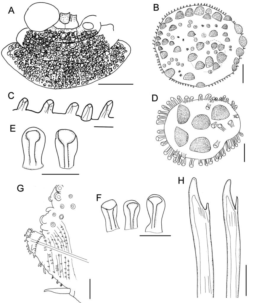
A small specimen (LACM 14774; 7.5 mm long, 3 mm wide) has morphological features present in larger specimens, such as the body shape, the pharynx is exposed and has 11 pairs of marginal papillae, with the midlateral ones smaller. The first elytra are markedly larger than the following ones, and it has many globular macro- and microtubercles, with surface echinulate, the fimbriae are slightly larger than 2 times longer than wide. Further, the parapodia are biramous and their integument is papillate, with few notochaetae, mostly 1 per ramus, and they are denticulate along a single side. The neurochaetae have a single accessory denticle, looking bifurcate, and lower neurochaetae tend to be sharper.
Taxonomic summary
Type material. Caribbean Sea, Virgin Islands. Holotype of Hermenia verruculosa Grube & Örsted, 1856 (ZMUC-1101), St. John, U.S. Virgin Islands, 6 Jun. 1846, coll. Krøyer. Smaller syntype of Polynoe nodosa Treadwell, 1902 (USNM 16013), Saint Thomas, U.S. Virgin Islands, USFCS Fish Hawk, Sta. 6079, 37-42 m, 6 Feb. 1899 (15 mm long, 3.5 mm wide); larger syntype (USNM 16014), Puerto Rico, Fajardo, US Steamer Fish Hawk, Sta. unumb., depth not given, probably intertidal, 17 Jan. 1899 (bent ventrally; first pair of elytra and left parapodia of chaetigers 2, 3 and 15-18, and right parapodium of chaetiger 20 previously removed (1 elytron, and 3 posterior ones left in container); paler dorsal transverse bands in chaetigers 8 and 10; venter with abundant tiny papillae. Body 25 mm long, 6 mm wide, 27 chaetigers).
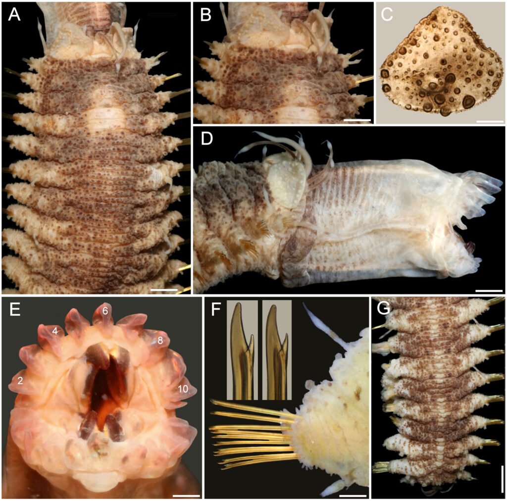
Distribution. Widely recorded along the tropical Western Atlantic, in shallow water, mixed, rocky, or coral bottoms. The indication for the Eastern Pacific (Salazar-Vallejo & Eibye-Jacobsen, 2012) was wrong. The record for the Arabian Sea (Wehe 2006) is shown below to belong to a different, newly described species (see below).
Additional material. Florida. One specimen (UF 1878), Gulf coast, N of St. Petersburg (28.59° N, 84.26° W), rock bottom, sponges, 29 m, 13 Mar. 2011, G. Paulay, M. Bemis & J. Moore, coll. complete, slightly bent ventrally; posterior end removed for molecular studies; no nuchal lappet; white spot rectangular, with paler areas in chaetiger 6; dorsal cirrostyles with swollen area white; anus position unknown; body 12 mm long, 3.5 mm wide, 26 chaetigers).
One specimen (UF 1879), same data as above (complete, slightly bent ventrally; pharynx exposed; first pair of elytra, and right parapodium of chaetiger 14 removed for observation (kept in container); no nuchal lappet; white spot rectangular, with paler areas in chaetiger 6; dorsal cirrostyles with swollen area white; anus terminal in chaetiger 26; body 21 mm long, 7 mm wide, 26 chaetigers).
One specimen (UF 1885), same data as above (complete, slightly bent ventrally; right elytron 1, and right parapodium of chaetiger 12 removed for observation (kept in container); no nuchal lappet; white spot rectangular, with paler areas in chaetiger 6; dorsal cirrostyles with swollen area white; anus terminal in chaetiger 26; body 24 mm long, 6 mm wide, 26 chaetigers).
Two specimens (USNM 17733), Dry Tortugas, Jun. -Jul. 1914, A.L. Treadwell, coll. (markedly bent ventrally; larger one with pharynx fully exposed, with 10-11 marginal papillae; body 25-30 mm long, 4.5-6.0 mm wide, 26 chaetigers).
Two specimens (USNM 46913), Tortugas,1930, W.L Schmitt, coll. (only 1 specimen in container; bent ventrally; chaetiger 6 with 3 white spots dorsally; 2 parapodia and first elytron from another specimen in container); body 30 mm long, 8 mm wide, 26 chaetigers).
Caribbean Sea. One specimen (ECOSUR 1309), University of Miami, Cruise P6806, RV Pillsbury, Southern Caribbean, off NE Venezuela, Sta. 709 (11°08.8’ N, 62°46.1’ W), 46 m, 19 Jul. 1968 (complete, anterior region almost completely brownish, with 1 middorsal small white spot in chaetiger 5, 2 laterals in chaetiger 6; no nuchal lappet; anus terminal in chaetiger 26; body 28 mm long, 6 mm wide, 26 chaetigers).
One specimen (ECOSUR 1310), University of Miami, Cruise P6802, RV Pillsbury, Nortwestern Caribbean, off Honduras, Sta. 629 (15°58’ N, 86°09’ W), 40 m, 21 Mar. 1968 (complete, anterior region with 1 middorsal small white spot in chaetiger 5, 2 laterals in chaetiger 6; no nuchal lappet; anus terminal in chaetiger 26; body 26 mm long, 7 mm wide, 26 chaetigers).
One specimen (ECOSUR 1311), Majagual, reef lagoon, rocks, 4 m, 6 Jun. 1998, M.A. Ruiz-Zárate, coll. (bent ventrally; with small narrow middorsal white and 2 lateral white spots in chaetiger 6; no nuchal lappet; anus terminal in chaetiger 26; body 18 mm long, 5 mm wide, 26 chaetigers).
Three specimens (ECOSUR 1316), Majagual, reef lagoon, rocks, 4 m, 6 Jun. 1998, M.A. Ruiz-Zárate, coll. (juveniles, bent ventrally, 1 with pharynx exposed, 10 pairs of marginal papillae; with wide middorsal white spot in chaetigers 4-5, and 2 lateral white spots in chaetiger 6; no nuchal lappet; anus terminal in chaetiger 26; body 8.1-8.5 mm long, 2.0-2.1 mm wide, 26 chaetigers).
One specimen (ECOSUR 3289), Majagual, Quintana Roo, México, reef lagoon, 4 m 6 Jun. 1998, M.A. Ruiz-Zárate, coll. (bent ventrally; pharynx exposed, 11 pairs of marginal papillae; 3 round white spots in chaetiger 6, anus terminal in chaetiger 26; body 13 mm long, 4 mm wide, 26 chaetigers).
One specimen (ECOSUR 3289), Punta Nizuc, Quintana Roo, México, 4 m, 10 Feb. 2001, P. Salazar-Silva, coll. (bent ventrally; with white middorsal band in chaetiger 5, wide transverse band in chaetiger 6; no nuchal lappet; anus terminal in chaetiger 26; body 11 mm long, 3 mm wide, 26 chaetigers).
One specimen (LACM 14763), British Virgin Islands, Guana Island, Muskmelon Bay, off Crab Cove (18.48° N, 64.57° W), reef slope coral heads, 10-16 m, 13 Jul. 2000, G. Hendler, T. Zimmerman, J. Martin & R. Ware, coll. (bent ventrally, with salt particles adsorbed on body; chaetigers 5-6 with a median rectangular white spot, and 2 smaller lateral ones on chaetiger 6; body 20 mm long, 6 mm wide, 26 chaetigers).
Two specimens (LACM 14774), British Virgin Islands, Guana Island, Pelican Ghut (18°28’36” N, 64°33’31” W), 6-12 m, G. Hendler, coll. (body 7.5-18.0 mm long, 3.0-6.5 mm wide, 26 chaetigers; smaller specimen features included in variation).
One specimen (LACM A44-39), Tortuga Island, RV Velero III, Sta. 44-39 (11°02’30” N, 65°14’45” W to 11°03’30” N, 65°14’00” W), 38-40 m, 21 Apr. 1939 (bent ventrally; chaetiger 6 with a median and 2 lateral white spots; body 23 mm long, 6 mm wide, 26 chaetigers).
Two specimens (LACM 147856), British White Bay, ARMS (18.3° N, 64.37° W), 9 m, 15 Jul. 2000, J. Zimmerman, J. Martin & R. Ware, coll. (almost colorless; both without nuchal hood, pharynx exposed, with 10 pairs of marginal papillae, body 6-8 mm long, 1.5-2.0 mm wide, 25-26 chaetigers).
One specimen (UMML 22.729a), University of Miami, Cruise P7006, Hispanola and Jamaica, RV Pillsbury, Sta. 1198 (17°49.4’ N, 76°12.3’ W), 29-37 m, 4 Jul. 1970 (bent ventrally; with 3 white spots, 1 in chaetigers 5-6, 2 laterals in chaetiger 6; without nuchal lappet; anus terminal in chaetiger 26; body 20 mm long, 6 mm wide, 26 chaetigers).
One specimen (UMML P979), University of Miami, Cruise P6907, Antillean Arc, Leeward Islands, RV Pillsbury, Sta. 979 (17°51’ N, 62°39’ W), 37 m, 22 Jul. 1969 (anterior fragment; without nuchal lappet; colorless, 10 mm long, 5 mm wide, 16 chaetigers).
One specimen (USNM 46916) Ascención Bay, Quintana Roo, Mexico, Central Part of Nicchehabin Reef., 1.2-1.8 m, Apr. 1960, E.L. Bousfield, coll. (slightly twisted; brownish, white spot in chaetiger 6; posterior nephridial lobes brownish; body 19.5 mm long, 5 mm wide, 26 chaetigers).
One specimen (USNM 46917), Ascensión Bay, Nicchehabin Reef., Quintana Roo, México, 21-19 m, 13 Apr. 1960, E.L. Bousfield, coll. (bent ventrally; dorsum with 3 white spots in chaetiger 6, chaetiger 5 with a median spot; body 28 mm long, 6 mm wide, 26 chaetigers).
One specimen (USNM 46920) Majito Reef, Puerto Rico, 0.3-0.6 m, 9 Mar. 1967, M.E. Rice, coll. (bent laterally; median segments swollen; body 20 mm long, 6 mm wide, 26 chaetigers).
Two specimens (USNM 50112), Carrie Bow Cay, Belize, 30 m, 11 Jun. 1972, M.E. Rice, coll. (bent ventrally; pharynx fully everted, 11-12 marginal papillae; body 16-21 mm long, 4-7 mm wide, 25-26 chaetigers).
One specimen (ZMUC-1102), St. Croix Island, H. Riise, coll. (no further data; prostomium retracted into second segment, without palps; body 19 mm long, 6.5 mm wide, 25 chaetigers).
Remarks
Hermenia verruculosa Grube & Örsted in Grube, 1856 differs from other species in the genus (see Hermenia key below)because it has a subrectangular dorsal white spot; segment 2 wide among the elytrophores, not projected on the prostomium as a nuchal lappet, elytrophores not expanded, dorsum with prominent globular densely packed tubercles; between segments 4 and 5 there is a dorsal small spot diffuse to well defined of unpigmented tubercles; venter wrinkled with abundant short thin papillae; elytra fleshy, rounded, attached firmly. The first pair of elytra is larger than the middle and posterior ones. All elytra with macrotubercles semispherical, spinous, unpigmented on the first pair of elytra, on subsequent elytrae reddish. Parapodia short, neuropodia diagonally truncate with an incipient prechaetal lobe. Neurochaetae with 1 accessory tooth and notochaetae absent in most of the parapodia. Pharynx everted with 11 pairs of marginal papillae and 2 pairs of jaws. The dorsal spot of unpigmented tubercles (Fig. 2F) is herein considered as distinctive of H. verruculosa.
Hermenia verruculosa has been recorded from different localities in the Grand Caribbean (Fauvel, 1953b; Horst, 1922; Bellan, 1964); however, the characterizations were short, often without illustrations, and the specimens are not available. Ebbs (1966) recorded 2 specimens from a coral patch of Margot Fish Shoal, Miami, Florida, as H. verruculosa, and his description referred red pigmentation; these specimens are colorless now, and the tubercles are white. On the other hand, part of Ebbs’ material corresponds with the features of H. verruculosa (UMML 150), whereas another lot (UMML 22:149) includes what we regard as an undescribed species described below.
Hermenia acantholepis (Grube, 1876) restricted
(Figs. 3, 4)
Polynoe acantholepis Grube, 1876: 61.
Polynoe (Lepidonotus) acantholepis: Grube, 1878: 24, Pl. 2, Fig. 1 (Samoa y Philippines).
Lepidonotus acantholepis: Herdman & Hornell, 1903: 25 (Ceylan, currently Sri Lanka, 82-92 m, in coral); Fauvel, 1922: 490-491, Fig. 1 (Houtman Abrolhos, Indian Ocean, in coral reef).
Hermenia acantholepis: Seidler, 1923: 262; Seidler, 1924: 94-95 (North West of Madagascar); Monro, 1924: 39-40, Figs 2-3 (Goto Island, Japon); Pruvot, 1930: 11-13, Pl. 1, Figs 27-32 (syn.); Fauvel, 1932a: 16-17 (Indian Ocean); Fauvel, 1947: 16-17, Fig. 12 (syn.), New Caledonia, South Pacific; Fauvel, 1953a: 38, Fig. 14a, b (Ceylan currently Sri Lanka); Pettibone, 1975: 239-241, Fig. 3 (partim, Fig. 4 corresponds to H. mezianei sp. nov., see below); Hanley & Burke, 1991: 62-64, Fig. 19A-G (Chesterfield Islands, New Caledonia, coral shallow water to 69 m, coral sand).
Diagnosis. Hermenia with body subrectangular; first and last pairs of elytra larger, overlapping, first 3 pairs larger than following ones; median elytra circular covering adjacent segments; elytral tubercles globular, with a basal hump; dorsal integument white, almost smooth, with thin papillae; segment 2 briefly projected over prostomium as a small nuchal lappet; neurochaetae tridentate.
Description. Holotype (ZMH 504) complete, mature female; dorsum wrinkled, globular tubercles scarce, whitish; venter wrinkled, without papillae; body depressed, 24 mm long, 6.5 mm wide, 26 chaetigers.
Prostomium in bad condition, wider than long, partially covered by segment 2; facial tubercle round; 2 pairs of eyes, both almost unpigmented. Median antenna with ceratophore cylindrical, long, inserted frontally; ceratostyle long, thick, surface smooth, without papillae; subdistally swollen, tip filiform. Lateral antennae with ceratophores thin, ceratostyle shorter, similar in shape to median antenna. Palps thick, without pigmentation, surface with rows of short papillae.
Tentacular segment not visible dorsally, tentaculophores thick, without chaetae; tentacular cirri similar in shape to median antennae. Segment 2 with nuchal lappet. Elytrophores expanded, not covering tentaculophores.
Elytra small, not overlapped laterally nor covering dorsum; elytra of anterior and posterior segments larger than elytra of middle segments, first pair of elytra round (Fig. 3C), second pair reniform (Fig. 3A); median and posterior elytra round (Fig. 3E), covering at least half width of adjacent segments. Elytral surface with tubercles and abundant filiform papillae. Tubercles abundant, ovoid, spinous, basally bulbous, projected beyond elytral margin (Fig. 3B, D). Elytra of median and posterior segments with marginal macrotubercles thinner, compressed (Fig. 3E-F), mostly brownish.
Parapodia with notopodia reduced, cylindrical ridge over neuropodia. Neuropodia thick, surface with transverse wrinkled rows, prechaetal lobe truncate, slightly larger than postchaetal lobe, distally with short papillae.
Dorsal cirri short, not longer than neuropodia, expanded subdistally, tips short filiform, similar in shape to antennae. Cirrophore cylindrical, short. Ventral cirri short, basally thick, tapered into fine tips, surface smooth. Nephridial papillae thick, short, distally blunt along chaetigers 6-25.
Notochaetae of anterior and middle segments short, scarce, upper region long, tapered into fine tip, absent in posterior segments. Neurochaetae thick, with striae; upper region short; tips thick, slightly curved, with 2 short, subdistal accessory teeth (Fig. 3G).
Posterior region tapered, blunt; pygidium with anus dorsal between chaetigers 25 and 26, anal cirri missing (thin, distally swollen, as long as last segment).
Variation. One specimen recently collected from Indonesia (UF 41) has a body almost pure white with brownish elytra (Fig. 4A); first 3 pairs of elytra larger than median ones, progressively smaller, such that the third is about twice as large as the fourth. The prostomium is white, with darker ceratophores and a basal medial region of ceratostyles, with a small dark band before swollen areas (Fig. 4B); eyes are black, of similar size, anterior eyes in the widest prostomial area, posterior ones towards the posterior margin. The nuchal lappet is truncate, well defined (Fig. 4B). The elytra have brownish macrotubercles, larger ones are marginal, with a basal swollen area, and globular microtubercles, more abundant along the inner anterior region (Fig. 4C). Parapodia biramous with small notochaetae (Fig. 4D, inset). Neurochaetae brownish with darker core, each with 2 subdistal teeth, often of similar size but different width (Fig. 4E). The posterior region is slightly tapered, with last pair of elytra slightly larger than preceding ones (Fig. 4F); anus dorsal, in posterior margin of chaetiger 25, anal cirri thin, resembling dorsal cirri, as long as last segment.
Taxonomic summary
Type material. Holotype of Polynoe acantholepis Grube, 1876 (ZMH 504), Upolu, Philippines.
Distribution. Indian Ocean and Western Pacific (Horst, 1917; Monro, 1939; Hanley & Burke, 1991; Imajima, 1997), in shallow mixed bottoms.
Additional material. Sri Lanka. One specimen (BMNH 1973:12), Talili, 73 m, no further data (dorsum wrinkled, with few tiny tubercles; venter with small papillae; first and second pair of elytra covering prostomium; elytral macrotubercles projected beyond margin, other elytra with marginal papillae filiform; notopodia small, with an acicular papilla).
Maldives. One specimen (BMNH 1941.4.4.195), Felidu, J.S. Gardiner, coll. (dorsum pale color, wrinkled with few papillae; notopodia short lobes; dorsal papillae short, compressed; venter with abundant short papillae; elytra of middle segments smaller than those of anterior segments, but larger than posterior ones).
Andaman Sea. Two specimens (LACM 2831963), juveniles, International Indian Ocean Expedition, RV Anton Bruun, Sta. 29 (11°23’ N, 93°31’ E), 55-40 m, 28 Mar. 1963 (1 dried-out; complete, whitish, cephalic appendages lost; elytra mostly white, barely compressed; nuchal lappet indistinct after eversion of pharynx; 11 pairs of marginal papillae; left parapodium of chaetiger 12 removed for observation kept in container; body 8 mm long, 2.5 mm wide, 26 chaetigers).
Indonesia. One specimen (UF 41), Sulawesi (Celebes Island), southern outer barrier reef (0.49° S, 122.07° E), 1-3 m, 22 Sep. 1999, G. Paulay, coll. (bent ventrally; body white, corrugated, pilose; elytra brownish, marginal macrotubercles L-shaped, internal lobe shorter; first elytra and left parapodium of chaetiger 14 removed for observation, kept in container; nuchal lappet distinct; dorsal cirrostyles with swollen area white; anus in chaetiger 25; body 23 mm long, 6 mm wide, 26 chaetigers).
Philippines. One specimen (CAS 187233), Hearst Philippine Biodiversity Expedition 2011, Luzon, Batangas Province, Mabini (Calumpan Peninsula), Maricaban Strait, Arthur’s Rock (13.70° N, 120.87° E), 16 m, 10 May 2011, A. Hermosillo, coll. (bent ventrally; body dirty white, first elytra whitish, all others brownish; first 3 and last elytra with marginal macrotubercles compressed, basally expanded (L-shaped); nuchal lappet short; dorsal cirrostyles with swollen areas white; anus in chaetiger 25; body 43 mm long, 9 mm wide, 26 chaetigers).
One specimen (CAS 214669), Verde Island Passage Expedition 2015, Mindoro, Oriental Mindoro Province, Puerto Galera, Shipyard Dive Site (13.52° N, 120.96° E), 6.5-16.0 m, sandy mud, 12 Apr. 2015, C. Piotrowski, coll. (partially dehydrated; middorsal area grayish, laterally white, elytra elytra brownish; first 3 and last elytra with marginal macrotubercles compressed, basally expanded (L-shaped); nuchal lappet distinct; dorsal cirrostyles with swollen areas white; anus between chaetigers 25-26; body 18.5 mm long, 5 mm wide, 26 chaetigers).
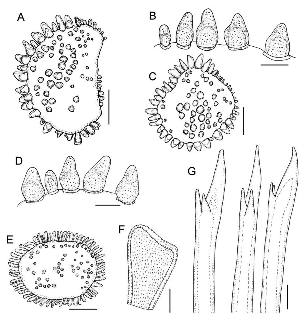
Papua New Guinea. One specimen (MNHN IA 2015-1924), Kavieng 2014 Expedition, New Ireland, RV Alis, Sta. DW4492 (02°25’23.99’’ S, 149°57’35.42’’ E), 112-140 m, 6 Sep. 2014 (bent ventrally, dried-out; first left elytron without macrotubercles along anterior inner area; median and posterior elytra circular, last pair larger than previous one; body 37 mm long, 7 mm wide, 26 chaetigers).
Coral Sea. One specimen (MNHN IA 2023-19), Cruise CORAIL 2, RV Coriolis, Sta. DW31 (19°24’51.59’’ S, 158°45’1.81’’ E), 57 m, 23 Jul. 1988, B. Richer de Forges, coll. (complete, slightly bent ventrally, first left elytron without macrotubercles along anterior inner area; median and posterior elytra circular, last 2 pairs larger than previous ones; body 22 mm long, 5.5 mm wide, 26 chaetigers).
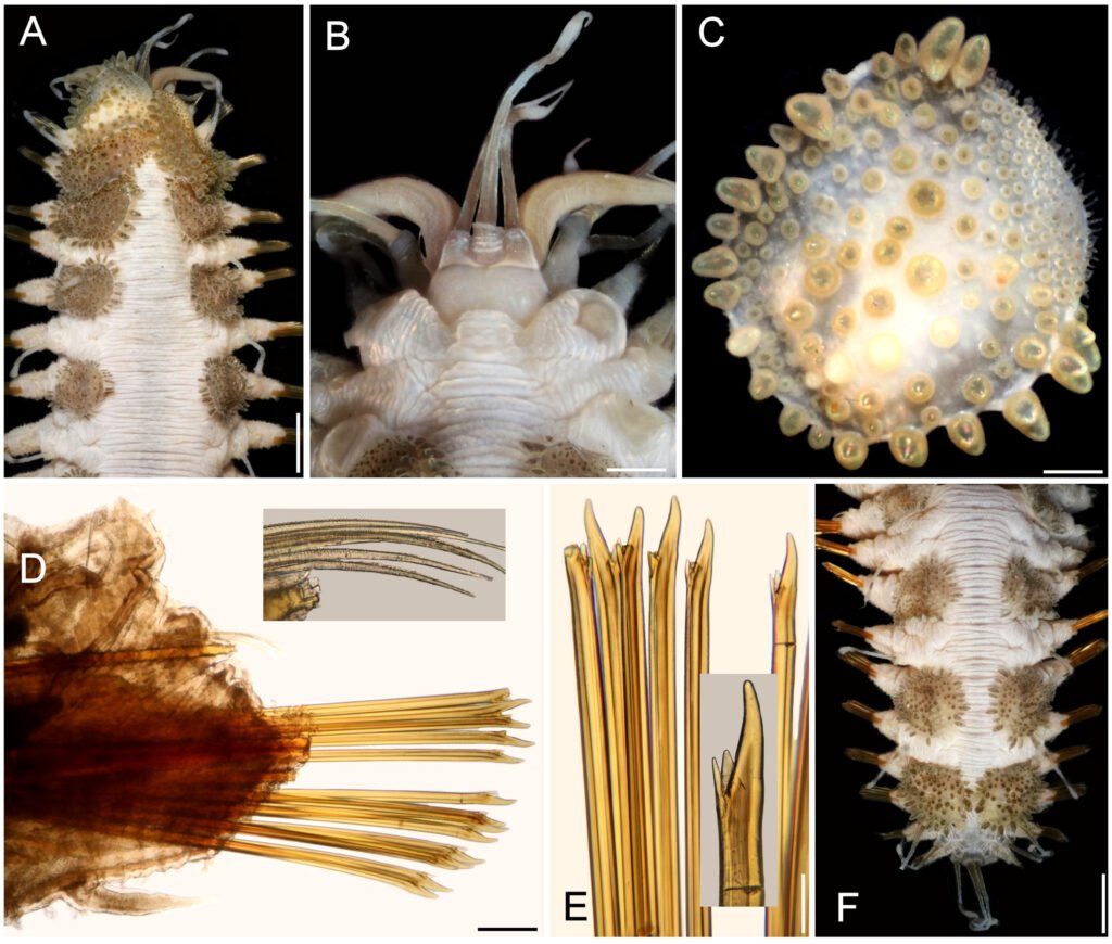
Japan. One specimen (BMNH 1925.1.28.4-5), Goto Island, no further data (dorsum wrinkled without tubercles or papillae; dorsum smooth; notopodia cylindrical ridges; coelom with numerous oocytes).
New Caledonia. One specimen (MNHN IA 2023-57), Musorstom Cruise LAGON, Yaté Sector, RV Vauban, Sta. DW642 (21°54’12.0024’’ S, 166°42’12.0204’’ E), 44-47 m, 7 Aug. 1986, B. Richer de Forges, coll. (complete, slightly bent ventrally, first left elytron without macrotubercles along anterior inner area; median and posterior elytra circular, last pair larger than previous ones; body 21 mm long, 6 mm wide, 26 chaetigers).
One specimen (MNHN IA 2023-58), Musorstom Cruise LAGON, Yaté Sector, RV Vauban, Sta. DW737 (22°08’23.99’’ S, 166°59’06’’ E), 49-50 m, 12 Aug. 1986, B. Richer de Forges, coll. (complete, slightly bent ventrally, first left elytron without macrotubercles along anterior inner area; median and posterior elytra circular, last pair larger than previous ones; body 17.5 mm long, 5.5 mm wide, 26 chaetigers).
Remarks
Hermenia acantholepis differs from H. verruculosa by having a depressed body; segment 2 wide projected on the prostomium as a short nuchal lappet; dorsum with transverse wrinkled ridges, tubercles small, flattened, scarce. Venter smooth, without papillae. Elytra with 2 kinds of tubercles, bulbous-ovoid basally and larger around margin. In earlier species diagnoses the marginal macrotubercles have been regarded as ovoid, but they are roughly bottle-shaped, with a basal swollen area; H. acantholepis is also distinguished by its neurochaetae because they have 2 subdistal accessory teeth, and notochaetae are present along most notopodia.
Pruvot (1930: 11) and Fauvel (1947: 17) noted that H. acantholepis has a milky white body, with brownish elytra, and dorsal cirri with brownish bases. Pruvot (1930: 13) also noted 2 varieties: the western one found from Sri-Lanka to the Philippines with very small elytra (matching H. neoverruculosa Pettibone, 1975, see below), and an eastern one, found in New Caledonia and Samoa, with larger elytra (matching the current H. acantholepis).
Hermenia neoverruculosa Pettibone, 1975
(Figs. 5, 6)
Hermenia acantholepis: Fauvel, 1932b: 132 (Gulf of Suez, Read Sea); Fauvel, 1933: 41 (Gulf of Suez, Read Sea); Wehe, 2006: 79, Fig. 13a-c. (non Grube, 1876; Red Sea).
Hermenia neoverruculosa Pettibone, 1975:242-245, Figs 5-6 (syn.).
Diagnosis. Hermenia with body subrectangular; first and second pair of elytra overlapping; dorsal integument with abundant globular tubercles, often with black core; segment 2 with nuchal lappet wide, round; median and posterior elytra with black macrotubercles; neurochaetae tridentate.
Description. Holotype (BMNH 1941.4.4.197) complete, body depressed, subrectangular, 30 mm long, 6.5 cm wide, 26 chaetigers. Dorsum with transverse rows of globular tubercles with darker cores, larger along anterior and posterior segments. Tubercles light brown, except on segments 3-4, where some tubercles are whitish, without pigmentation, forming a small, diffuse middorsal spot. Venter pale, wrinkled, pubescent.
Prostomium bilobed (Fig. 5A), wider than long, not retracted into segment 2; facial tubercle round, pale. Eyes black; anterior eyes directed anteriorly, on the widest part of the prostomium, subdermal; posterior eyes near posterior margin, darker, slightly larger Fig. 6B). Median antenna with ceratophore inserted frontally, thick, surface with papillae, ceratostyle tubular, 2 times as long as prostomium length, subdistally swollen, tip filiform, surface smooth, with dark bands; lateral antennae with ceratophores cylindrical, short, about as long as prostomium; ceratostyles shorter, resembling median antenna. Palps missing.
Tentacular segment not visible dorsally, tentaculophores thin, long, with scarce, short chaetae. Tentacular cirri thin, long, resembling antennae, surface smooth.
Segment 2 narrow with a wide rounded nuchal lappet. First pair of elytrophores reaching bases of tentaculophores. Nephridial papillae not visible along anterior segments, distinct from chaetiger 7, longer along median and posterior segments.
First 2 pairs of elytra larger than following ones; elytron 3 slightly larger than elytron 4; first pair of elytra overlapped dorsally; elytral surface with macrotubercles blackish (Fig. 5B), or pale, and papillae; macrotubercles scattered, ovoid, short to elongate, blunt, spinous, micropapillae cylindrical, abundant (Fig. 5C), thicker along margin. Elytra of median and posterior segments small (Fig. 5D), macrotubercles black, with abundant cylindrical papillae on surface and along margins (Fig. 5E).
Parapodia with notopodia reduced to acicular lobe, acicular papilla present (Fig. 5F). Neuropodia thick, robust, distally with small papillae, and small prechaetal and postchaetal lobes with long papillae, postchaetal lobe larger than prechaetal one; dorsal surface with transverse rows of globular pale tubercles. Dorsal cirri thin, smooth, short, not reaching neurochaetae tips, same shape as antennae; cirrophore short, cylindrical. Ventral cirri short, thin, not reaching the lower tip of the neurochaetal lobe.
Notochaetae thin, short, 2-3, laterally denticulate capillaries. Neurochaetae thick, upper region short, main fang long, thick, slightly curved, more curved in posterior segments, accessory teeth short, 1/4 as long as main fang. Second parapodia with thin neurochaetae, tips entire with 3 long spines. Median parapodia with neurochaetae often with 2 accessory teeth, sometimes 1 broken (Fig. 5G).
Posterior region tapered, truncate; pygidium with anus dorsal, anal cirri lost.
Variation. One specimen (UF 3985) has body grayish, dorsal tubercles with cores slightly darker, better defined in intersegmental areas; first elytra pale with macrotubercles blackish, other elytra grayish with dark macrotubercles; first and second pair of elytra of similar size, second pair about 3 times as large as third pair (Fig. 6A); following elytra small, round, with black macrotubercles.
Prostomium pale, with ceratophores blackish with pigmentation extended along anterior prostomial areas, ceratostyles brownish, with a wide brownish band before enlarged pale area, tips pale (Fig. 6B); nuchal lappet barely developed, truncate. First elytron (Fig. 6C) with marginal macrotubercles lobate, not basally expanded, inner macrotubercles globular, shorter, blackish and paler ones (Fig. 6C).
Parapodia biramous (Fig. 6D) with few notochaetae (Fig. 6D, inset); neurochaetae abundant, brownish and paler, with darker cores (Fig. 6E), each with 2 fragile, tapered accessory teeth, sometimes with a single denticle left (Fig. 6E, inset), or all broken. Posterior region tapered; last pair of elytra as large as preceding ones, with black macrotubercles; anus dorsal between chaetigers 25-26, anal cirri thin, delicate, as long as last chaetiger (Fig. 6F).
Taxonomic summary
Type material. Republic of Mauritius. Holotype of Hermenia neoverruculosa Pettibone, 1975 (BMNH 1941.4.4.197), Cargados Carajos, 55 m, Sea Lark Expedition, 28 Aug. 1905, J.S. Gardiner, coll.
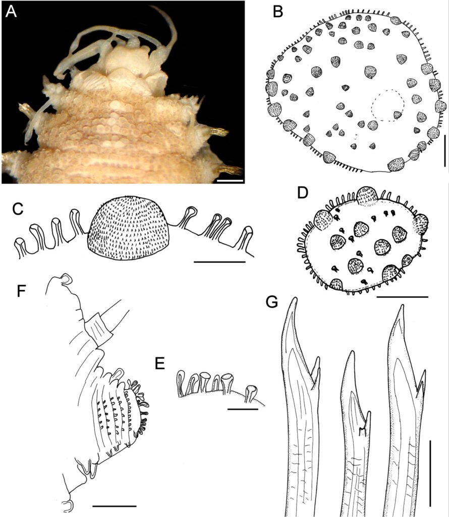
Distribution. Indian Ocean to Western Pacific, in shallow water mixed bottoms.
Additional material. Red Sea. One specimen (MNHN A403), Mission Dollfus en Égypte 1927-1929, Sta. 24, ‘bloc des vermets’ (probably intertidal Dendropoma vermetid mass, see Ben-Eliahu 1975), 30 Dec. 1928, R.P. Dollfus, coll. (complete, bent ventrally, partially dehydrated, integument damaged, middorsally eroded, with fine sediment particles laterally; dorsum with tubercles; all elytra on site, with fine sediment particles, median and posterior elytra circular; anus between chaetigers 25-26; body 14.5 mm long, 4 mm wide, 26 chaetigers).
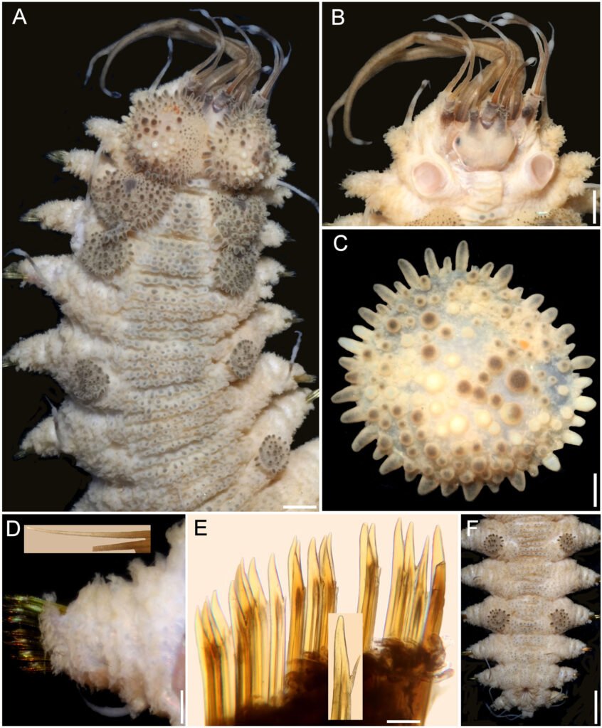
One specimen (MNHN A894), Mission Dollfus en Égypte 1927-1929, Sta. 24, ‘bloc des vermets’ (probably intertidal Dendropoma vermetid mass, see Ben-Eliahu 1975), 30 Dec. 1928, R.P. Dollfus, coll. (complete, breaking in 2 parts, integument damaged, almost completely detached from body wall; dorsum with tubercles; 2 anterior elytra and right parapodium of chaetiger 12 previously removed, kept in container; most elytra on site, median and posterior ones circular; anus between chaetigers 25-26; body 18.5 mm, long, 5 mm wide, 26 chaetigers).
Papua New Guinea. One specimen (MNHN IA 2017-3596), Papua Niugini Expedition, W. Wongat Island, Sta. PR108 (05°08’04.44” S, 145°49’29.21” E), 2-30 m, 26 Nov. 2012 (complete, bent ventrally; all elytra on site, median elytra circular, smaller than segment width; anterior end markedly retracted, nuchal lappet not seen; dorsal tubercles globular, with black core; venter pubescent; anus dorsal between chaetigers 25-26; body 45 mm long, 8 mm wide, 26 chaetigers).
One specimen (UF 3985), Madang Province, BilBil Island (5.2962° S, 145.7822° E), outer reef, 13 m, 12 Nov. 2012, B. Faure, R. Ibik & P.-H. Kuo, coll. (complete, slightly bent laterally; first pair of elytra and right parapodia of chaetigers 10 and 12 removed for observation, kept in container; nuchal lappet distinct; dorsal tubercles globular with black core; venter pubescent; anus dorsal between chaetigers 25-26; body 40 mm long, 7 mm wide, 26 chaetigers).
One specimen (UF 3986), Madang Province, University Road (5.22° S, 145.79° E), 15 m, 12 Nov. 2012, B. Faure, R. Ibik & P.-H. Kuo, coll. (complete, juvenile, markedly bent ventrally after removal of left parapodia of chaetigers 11-16; not dissected to avoid further damage; elytra 2-6 with black spot in insertion area; elytra of median and posterior chaetigers with macrotubercles pale and black; nuchal lappet short; dorsal tubercles globular with black core, better defined intersegmentally; venter pubescent; anus dorsal between chaetigers 25-26; exposed enteron with globular, longer than wide caeca; body 14 mm long, 2.5 mm wide, 26 chaetigers).
Remarks
Hermenia neoverruculosa resembles H. verruculosa because both have dorsal globular tubercles, elytra with spinous macrotubercles and papillae. However, H. neoverruculosa differs from H. verruculosa in that its dorsal tubercles are shorter and densely packed, its venter is smooth, segment 2 is dorsally narrow between the first pair of elytrophores, and projected as a nuchal lappet over the prostomium, notochaetae are small in most parapodia, and neurochaetae have mostly 2 accessory teeth.
Hermenia neoverruculosa had been recorded only in the Indian Ocean, including D’arros Island (Monro, 1924:40), and the Seychelles (Monro, 1939:169). Pettibone (1975) recorded both materials and the features match the species.
Hermenia chuarae sp. nov.
(Fig. 7)
http://zoobank.org/urn:lsid:zoobank.org:act:59B0411C-59EB-4533-BAC3-5DE3698C850F
Hermenia acantholepis: Chuar et al., 2021: 64-65, Fig. 3G (non Grube, 1876 (Sunda Strait, Indonesia, 448-469 m, on sediment).
Diagnosis. Hermenia with body subrectangular; first and second pair of elytra overlapping; dorsal integument with abundant depressed tubercles, with pale core; segment 2 with nuchal lappet wide; median and posterior elytra with pale and brownish macrotubercles; neurochaetae tridentate.
Description. Holotype (MMMM 000) complete, body depressed, subrectangular, slightly bent laterally, 37 mm long, 6 mm wide, 26 chaetigers. Dorsum with transverse rows of depressed tubercles (Fig. 7A), core pale, of similar size along body; tubercles brownish, darker basally. Venter pale, wrinkled, with abundant filiform papillae.
Prostomium bilobed, about as wide as long, slightly retracted into segment 2; facial tubercle not visible dorsally, pale, with a median globular tubercle. Eyes black; anterior eyes about 2 times as large as posterior ones, directed anteriorly, on the widest part of the prostomium (Fig. 7B); posterior eyes near posterior margin. Antennae, palps, and tentacular cirri directed posteriorly. Median antenna with ceratophore papillate, inserted frontally, 2 times as wide and longer than laterals, ceratostyle about 2 times as long as prostomium, thin, subdistally swollen, swollen region pale, darker along it, tip thin, dark; lateral antennae with ceratostyles 1.5 times as long as prostomium, shorter than median one, with similar pigmentation pattern. Palps tapered, papillate, subdistally with a black ring, tips pale.
Tentacular segment indistinct dorsally, tentaculophores thin, long, with a single short chaeta. Tentacular cirri longer than median antenna, shorter than palps, with a similar pigmentation pattern to the antennae.
Segment 2 narrow with a wide rounded nuchal lappet. First pair of elytrophores reaching bases of tentaculophores. Nephridial papillae not visible along anterior segments, distinct from chaetiger 7, longer along median and posterior segments, often with marginal papillae.
First 3 pairs of elytra larger than the following ones, elytron 3 slightly larger than twice elytron 4. First pair of elytra overlapped dorsally; elytral surface with macrotubercles white and brownish (Fig. 7C), and papillae indistinct; macrotubercles short, globular to elongate, blunt. Elytra of median and posterior segments small, macrotubercles pale or brownish, with abundant papillae along margins.
Parapodia with notopodia reduced to acicular lobe (Fig. 7D), acicular papilla present. Dorsal cirri thin, smooth, short, not reaching neurochaete tips, resembling antennae; cirrophore short, cylindrical. Neuropodia thick, robust, distally with small papillae, and small prechaetal and postchaetal lobes with long papillae; prechaetal lobe larger than postchaetal one. Ventral cirri short, tapered, reaching the lower tip of the neurochaetal lobe.
Notochaetae thin, short, 3-4 laterally denticulate capillaries (Fig. 7D, inset). Neurochaetae thick, upper region short, main fang long, slightly falcate, accessory teeth short, 1/3 as long as main fang (Fig. 7E). Median parapodia with neurochaetae often with 2 accessory teeth, sometimes 1 denticle broken.
Posterior region tapered, truncate (Fig. 7F); pygidium with anus dorsal, anal cirri long, resembling antennae, about as long as last 3 chaetigers.
Taxonomic summary
Type material. Sunda Strait, Indonesia. Holotype (MZB Pol. 300), South Java Deep-Sea Biodiversity Expedition 2018, RV Baruna Jaya VIII, Sta. DW17 (06°07.33’ S, 105°00.76’ E to 06°07.22’ S, 105°00.86’ E), 448-469 m, 26 Mar. 2018.
Distribution. Only known from the Sunda Strait, Indonesia, in bathyal depths.
Etymology. This species is named after Miss Cheah Hoay Chuar. She is a polychaete taxonomist at the National University of Singapore, in recognition of her involvement in the South Java Deep Sea Biodiversity Expedition 2018, and because she kindly allowed us to study the holotype for this species.
Remarks
Hermenia chuarae sp. nov. resembles H. neoverruculosa, originally described from the Cargados Carajos Archipelago, Republic of Mauritius, Indian Ocean. Both species have a dorsum grayish with transverse rows of tubercles and elytral macrotubercles globular, non-L-shaped. However, they differ because H. chuarae has dorsal tubercles depressed, without black cores, and the median and posterior elytra have pale and brownish macrotubercles, whereas in H. neoverruculosa the dorsal tubercles are globular with black cores, and its median and posterior elytra have black macrotubercles.
On the other hand, the holotype of H. chuarae is the deepest record for any Hermenia species, being collected in sediments at 448-469 m depth.
Hermenia mezianei sp. nov.
(Fig. 8)
http://zoobank.org/urn:lsid:zoobank.org:act:500F2A6D-2A63-44F5-8DAB-EDE4646B7DCB
Hermenia acantholepis: Fauvel, 1935: 281, 286 (Vietnam, Pacific Ocean); Fauvel, 1939: 256 (Vietnam, Pacific Ocean); Dawydoff, 1952: 90 (non Grube, 1876; Vietnam, Pacific Ocean).
Diagnosis. Hermenia with body blunt fusiform; only first pair of elytra overlapping, first 3 pairs larger than following ones; median elytra oval barely covering adjacent segments; elytral tubercles globular, with a basal hump; dorsal integument white, barely rugose anteriorly, with thin papillae; segment 2 barely projected over prostomium as a small nuchal lappet; neurochaetae 2 accessory teeth.
Description. Holotype (MNHN A398) complete, dorsum wrinkled, almost smooth, a few sparse tubercles and larger papillae anteriorly (Fig. 8A); left elytra 1, right elytra 1, 2, and right parapodia of chaetigers 2, 14, and 15 previously dissected (kept in container), venter smooth, without papillae; body depressed, 13.5 mm long, 4.5 mm wide, 26 chaetigers.
Prostomium partially retracted into following segment, subhexagonal, wider than long (Fig. 8B); facial tubercle not visible dorsally, low; 2 pairs of black eyes of similar size. Median antenna with ceratophore 2 times as wide and slightly longer than laterals, ceratostyle short, tapered (probably in regeneration); right lateral ceratostyle smooth, tapered, subdistally wider, longer than palps. Palps barely papillate.
Tentacular segment not visible dorsally, tentaculophores thick, without chaetae; right tentacular cirri asymmetrical, ventral ceratostyle one 2 times as long as dorsal one (probably in regeneration). Segment 2 was previously slightly dissected, with a short nuchal lappet. Elytrophores not covering tentaculopohores.
Elytra small, not overlapped laterally nor covering dorsum: first 3 elytra larger than median ones, elytra 1 and 2 of similar size, elytron 3 about half their size, elytron 4 and following ones slightly smaller than elytron 3, oval, wider than long, barely covering adjacent segments. Elytra surface with tubercles and sparse filiform papillae (Fig. 8C). Tubercles abundant, ovoid, spinous, some basally bulbous, most globular, projected beyond elytral margins; marginal tubercles progressively smaller in median and posterior segments, pale or brownish.
Parapodia with notopodia reduced, blunt conical ridge over neuropodia (Fig. 8D). Neuropodia thick, surface with transverse wrinkled rows, prechaetal and postchaetal lobes truncate, of similar size, with margin papillate.
Dorsal cirri long, reaching upper neurochaetae, subdistally swollen, brownish, tips long filiform, resembling antennae and tentacular cirri. Cirrophore very short, cylindrical. Ventral cirri short, tapered, surface smooth. Nephridial papillae globular, short, along chaetigers 6-25.
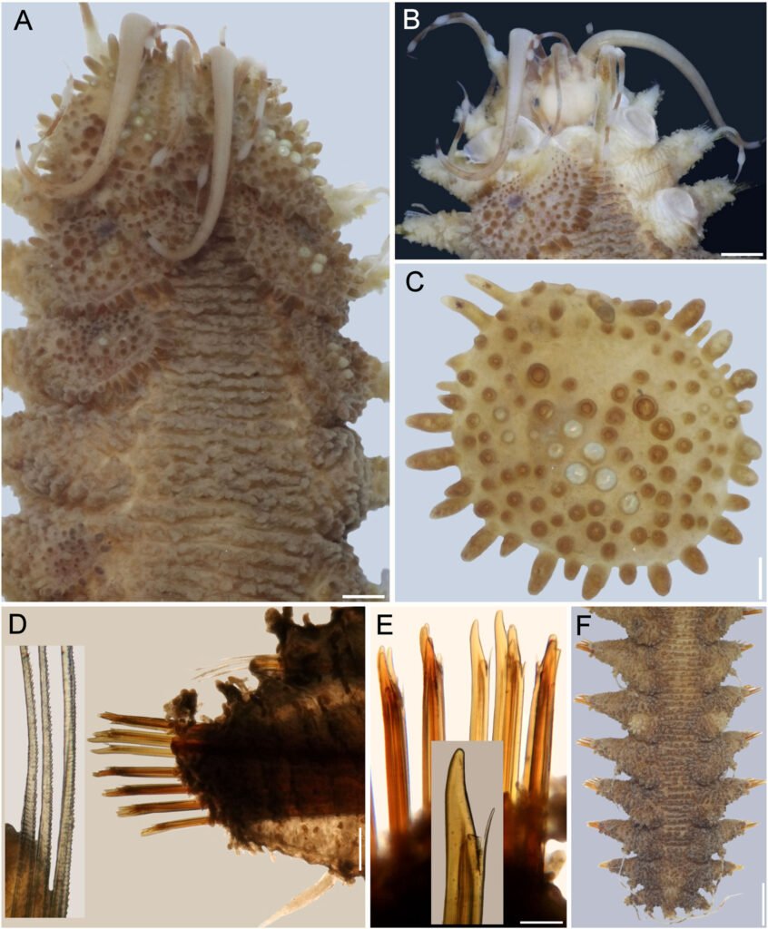
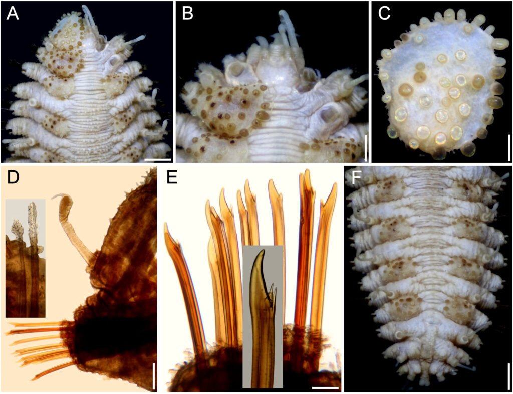
Notochaetae short, scarce, fragile, tips broken (Fig. 8D, inset), with impurities, marginally denticulate. Neurochaetae thick, smooth, upper region short; tips thick, slightly falcate, with 2 short, subdistal accessory teeth (Fig. 8E).
Posterior region tapered, blunt (Fig. 8F); last pair of elytra of similar size as preceding ones, pygidium with anus dorsal between chaetigers 25 and 26, anal cirri missing.
Taxonomic summary
Type material. Vietnam. Holotype (MNHN A398), Hón Lön Island (Honlohé, Ile Mamelles), By of Nha Trang, C. Dawydoff, coll. (no further data).
Distribution. Only known from Vietnam and Futuna Island (South Pacific Ocean), in substrates in platform-shelf depths.
Etymology. The specific epithet is after Dr. Tarik Meziane, curator of the Annelid collection in the Muséum National d’Histoire Naturelle, Paris, in recognition of the support he has kindly provided to our research projects.
Additional material. Futuna Island, Western Pacific, One specimen (MNHN IA 2023-45), Cruise MUSORSTOM 7, RV Alis, Sta. CP517 (14°13’23.99’’ S, 178°10’24.02’’ W), 223-235 m, 12 May 1992, P. Bouchet et al., coll. (partially dehydrated, markedly bent ventrally, integument tuberculate; first 3 pairs of elytra larger than following ones, third elytra about 2 times as large as fourth one; median and posterior elytra circular to oval, slightly wider than long, barely covering segment; last pair of elytra as large as previous one; not measured to avoid further damage).
Two specimens (MNHN IA 2023-48), Cruise MUSORSTOM 7, RV Alis, Sta. CP498 (14°18’54’’ S, 178°03’05.99’’ W), 105-160 m, 10 May 1992, P. Bouchet et al., coll. (integument tuberculate; first 3 pairs of elytra larger than following ones, third elytra about 2 times as large as fourth one; median and posterior elytra circular to oval, slightly wider than long, barely covering segment; last pair of elytra slightly larger than precedent one; body 18-28 mm long, 5.5-6.0 mm wide, 26 chaetigers).
Remarks
Hermenia mezianei sp. nov. resembles H. acantholepis restricted, by having a whitish, almost smooth integument, first 3 pairs of elytra larger than the following ones, each with marginal macrotubercles basally swollen, and trifid neurochaetae. Their main differences are the shape and size of the median and posterior elytra, the distribution of macrotubercles in the first elytra, and the type of macrotubercles in the median and posterior elytra. First, in H. mezianei the median and posterior elytra are oval, wider than long, barely covering adjacent segments, whereas in H. acantholepis they are circular and cover at least half of the adjacent segments. Second, the first elytra of H. mezianei have the anterior inner area with round macrotubercles, whereas there are no macrotubercles in the same area in H. acantholepis, only microtubercles. Third, macrotubercles in median and posterior elytra in H. mezianei are short, globular, mostly pale, barely projected from the elytral margin, whereas in H. acantholepis they are digitate, almost all brownish, markedly projected from the elytral margin.
Hermenia treadwelli sp. nov.
(Figs. 9, 10)
http://zoobank.org/urn:lsid:zoobank.org:act:9588D5E3-1895-4086-AD94-A650503CB7F7
Hermenia verruculosa: Treadwell, 1911: 9-11, Figs 23-26 (partim, nonGrube & Örsted in Grube, 1856; Dry Tortugas, Florida in dead coral); Pettibone, 1975: 235-238, Figs 1, 2 (syn., partim; only his specimens completely white along anterior chaetigers.
Diagnosis. Hermenia with body fusiform; segment 2 with short nuchal lappet; first pair of elytra bigger, not overlapping, other elytra tiny; dorsal integument with abundant dorsal tubercles, paler ones forming an inverted T-shaped spot in segments 5 or 5 anterior segments white, with pale tubercles; segment 2 with short projection over prostomium as a nuchal lappet; neurochaetae bidentate.
Description. Holotype (ECOSUR 1396) with body robust, depressed, fusiform, widest medially, 24 mm long, 6.5 mm wide, 26 segments. Dorsum covered with globular tubercles of different sizes, some larger than the others, larger in anterior and posterior segments, tubercles dark brown in anterior segments, paler towards posterior part in cirrigerous segments, giving an appearance of banding of dark segments alternating with pale ones. First 5 segments almost completely white (Fig. 9A). Venter with thick digitiform papillae.
Prostomium bilobed (Fig. 9B), retracted into the second segment. Two pairs of dark eyes, anterior pair on the widest part of the prostomium; posterior eyes covered by second segment. Palps robust with papillae, tapered, tips filiform (left palp lost). Three antennae, median antennae with ceratophore inserted frontally on prostomial lobe, about 2 times as wide as laterals, cylindrical, darker than prostomium, ceratostyles lost. Pharynx not everted.
First pair of elytra largest, round (Fig. 9C), covering prostomium, following elytra smaller; first pair of elytra with papillae digitiform, short, thick on the surface and along margin; elytral surface with many macrotubercles, present on elytrophore mark, larger towards margin. Elytra of median and posterior segments with abundant digitiform papillae on surface and along margin; macrotubercles thick, hemispherical, spinous.
Tentacular segment not visible dorsally; tentaculophores short, without chaetae; tentacular cirri thick, similar in shape and length as the median antenna. Segment 2 narrow between the first pairs of elytrophores, projected on the prostomium as a nuchal lappet. First pair of elytrophores expanded.
Parapodia biramous, truncate, dorsal surface with rows of globular tubercles (Fig, 9D). Notopodia short, acicular ridge covered with 1 blunt papilla (Fig. 10D, inset left). Neuropodia thick with prechaetal and postchaetal lobes reduced, each with abundant marginal papillae. Cirrigerous segments with dorsal cirri short, not surpassing neuropodia tips, surface smooth, similar in shape to antennae; cirrophore short, thick, with papillae; ventral cirri thin, short. Nephridial papillae visible from segment 7, thick, and becoming larger on posterior segments.
Notochaetae absent. Neurochaetae of median and posterior segments thick (Fig. 9D, insets above), upper region short with a long tooth, slightly curved, and a secondary straight denticle distant from each other. Parapodia of the second segment with neurochaetae thinner, of 2 kinds, some with long spines, tips entire, others with spines only subdistally.
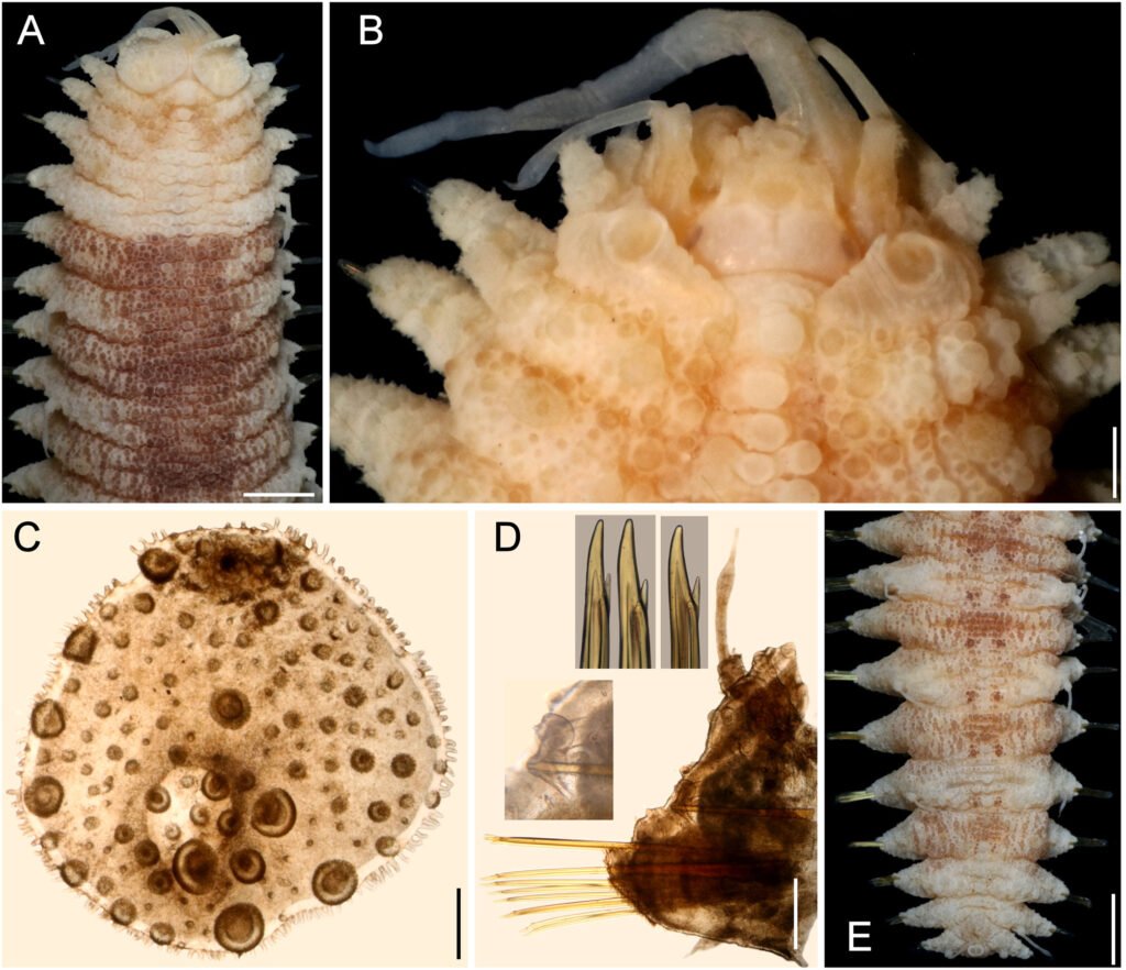
Posterior region pale, truncate (Fig. 9E); last pair of elytra as large as preceding ones, pygidum terminal, dorsal anus, anal cirri lost.
Variation. Other specimens have first elytra pale, and an anterior, inverted triangle spot along the dorsum of the chaetigers 3-5 (Fig. 10A). The prostomium retains dark-reddish pigmentation along ceratophores, and the median antenna ceratostyle, palps, and tentacular cirri are brownish, with pale swollen areas (Fig. 10B). The nuchal lappet is better defined as well.
The first elytron has globular macrotubercles, mostly brownish, with abundant marginal papillae and pale microtubercles along its surface (Fig. 10C). Parapodia biramous (Fig. 10D) with barely projected notopodia (Fig. 10D, left inset), and dorsal cirri with conical cirrophore (Fig. 10D, upper inset). Notochaetae broken and lost. Neurochaetae abundant, brownish (Fig. 10E), with 1 subdistal accessory denticle (Fig. 10E, insets).
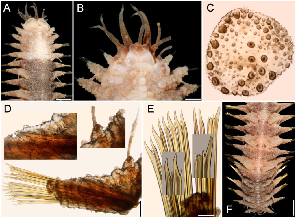
Posterior region banded (Fig. 10F), elytrigerous chaetigers with dorsal surface darker, cirrigerous chaetigers paler; pygidium with anus dorsal, between chaetigers 25-26, anal cirri lost.
Taxonomic summary
Type material. Caribbean Sea. Holotype (ECOSUR 1396), Chinchorro Bank, Cayo Norte, R/V Edwin Link, Sta. 2774 (18º45.63’ N, 87º15.84’ W), 55 m, August, 1990 E. Escobar, L. Soto, J.L. Villalobos, coll.
Distribution. Western Tropical Atlantic (Bahamas to Venezuela), in shallow mixed bottoms.
Etymology. The species is named to honor the late Dr. Aaron Treadwell in recognition of his contributions to the knowledge of different families of polychaetes.
Additional material. Northwestern Atlantic. One specimen (USNM 3296), USFCS Albatross, Sta. 2246 (39°56’45” N, 70°20’30” W), off New Jersey, U.S.A., Sta. 188, 220 m, 26 Sep. 1884 (posterior region bent ventrally; dorsum of chaetigers 2-5 with a discontinuous inverted T-shaped white spot; body 22 mm long, 5.5 mm wide, 26 chaetigers).
Bahamas. One specimen (USNM 16492), Holding Key, Andros Island, 13 May 1912, P. Bartsch, coll. (slightly bent laterally; chaetigers 2-5 with dorsum almost completely white; body 20 mm long, 5 mm wide, 26 chaetigers).
One specimen (USNM 46921), outer reef, point north of Clarencetown, Long Island, 15 May 1970, C. Riser, coll. (chaetigers 4-5 with a wide, inverted T-shaped white band, interrupted laterally; median and posterior nephridial lobes brownish; body 28.5 mm long, 5.5 mm wide, 26 chaetigers).
Florida. One specimen (USNM 17722), Tortugas, 1914, A.L. Treadwell, coll. (dorsum brownish, with inverted T-shaped wide band in chaetigers 4-5; body nephridial lobes from chaetiger 8, progressively larger posteriorly; 34 mm long, 7 mm wide, 26 chaetigers).
Caribbean Sea. One specimen (ECOSUR 9), Majagual, Quintana Roo, México, 6 Jun. 1998, M.A. Ruiz-Zárate, coll. (juvenile; slightly twisted; no dissected to avoid further damage; without nuchal lappet; anterior region with inverted T-shaped white spot along chaetigers 4-5; anus in chaetiger 26; body 11 mm long, 3 mm wide, 26 chaetigers).
One specimen (ECOSUR 1305), Majagual, Quintana Roo, México, 6 Jun. 1998, M.A. Ruíz-Zárate, coll. (juvenile, complete; bent ventrally; chaetigers 1-5 completely white; nuchal lappet distinct; anus terminal in chaetiger 26; body 11 mm long, 3.5 mm wide, 26 chaetigers).
One specimen (ECOSUR 1312), Xcacel, Quintana Roo, México, 17 Apr. 1996, S.I. Salazar-Vallejo & L.F. Carrera-Parra, coll. (complete; bent ventrally; pharynx exposed, 10 pairs of marginal papillae; chaetigers 1-5 completely white; nuchal lappet short; anus terminal in chaetiger 26; body 18 mm long, 5 mm wide, 26 chaetigers).
One specimen (ECOSUR 1318), Venezuela, Margarita Island, Los Testigos, seagrasses, 6 Jun. 1961 (partially dehydrated; anterior region with inverted triangle white spot along chaetigers 4-5; nuchal lappet distinct; anus in chaetiger 26; body 19 mm long, 5 mm wide, 26 chaetigers).
Two specimens (ECOSUR 1394), Punta Nizuc, Cancún, Quintana Roo, coral rocks, 1 Sep. 1997, S.I. Salazar-Vallejo, L.F. Carrera-Parra & M.A. Ruiz-Zárate, coll. (complete, fusiform; first 5 chaetigers almost completely white; nuchal lappet short; anus terminal in chaetiger 26; body 20-27 mm long, 5.5-7.5 mm wide, chaetigers).
One specimen (ECOSUR 1395), Majagual, Quintana Roo, reef lagoon, rocks, 18 Mar. 2002, S.I. Salazar-Vallejo, coll. (complete, fusiform; first 5 chaetigers almost completely white; nuchal lappet distinct; anus terminal in chaetiger 26; body 28.5 mm long, 7 mm wide, chaetigers).
One specimen (ECOSUR 2429), Punta Herradura, Quintana Roo, México, 28 Oct. 1997, P. Salazar-Silva, coll. (bent laterally; first right elytron and left parapodium of chaetiger 5 previously removed, kept in container; anterior region with inverted T-shaped white spot along chaetigers 4-5; anus prolapsed, in chaetiger 26; body 21 mm long, 5.5 mm wide, 26 chaetigers).
One specimen (LACM 14762), British Virgin Islands, Guana Island, Beef Island, long white beach at far west end of airport property, (18.448° N, 64.541° W), coral rubble, 1-2 m, snorkel, hand, 23 Jul 2000. T. Zimmerman, T. Haney, R. Ware, D. Cadien, coll. (barely bent ventrally, with salt particles adsorbed on body; chaetigers 4-5 with an inverted T-shaped white band; body 26.5 mm long, 7 mm wide, 26 chaetigers).
One specimen (LACM 147883), Jamaica, Saint Ann Bay, Bull Reef (18.735° N, 77.289° W), coral rubble and algae, 8 m, 2 Jun. 2006, K. Rawlinson, M. Bolanos, A. DuPont, A. Allan, J. Dunn & L. Harris, coll. (slightly bent ventrally, pharynx partially exposed; chaetigers 2-5 completely white dorsally; body 14.5 mm long, 3.5 mm wide, 26 chaetigers).
Three specimens (LACM 147910), British Virgin Islands, Guana Island, White Bay, ARMS (18.3° N, 64.37° W), 9 m, 15 Jul. 2000, J. Zimmerman, J. Martin & R. Ware, coll. (smaller ones almost colorless, largest bent ventrally, with an inverted whitish T-shaped spot along anterior chaetigers; body 7-26 mm long, 2.0-6.5 mm wide, 26 chaetigers).
One specimen (UMML 22.729b), University of Miami, Cruise P7006, Hispanola and Jamaica, RV Pillsbury, Sta. 1198 (17°49.4’ N, 76°12.3’ W), 29-37 m, 4 Jul. 1970 (bent ventrally; smaller one with inverted T-shaped white spot in chaetigers 2-5, anus terminal in chaetiger 26; body 15 mm long, 5 mm wide, 26 chaetigers).
One specimen (UMML P341), University of Miami, Cruise 6607, Panama to Venezuela, R/V Pillsbury, Sta. 341 (09°02’ N, 77°02’ W), 44 m, 9 Jul. 1966 (anterior region with an inverted T-shaped spot in chaetigers 2-5; first left elytron and left parapodia of chaetigers 3, 4, 13 previously removed (elytron and 1 parapodium kept in container); anus in chaetiger 26; body 15 mm long, 5 mm wide, 26 chaetigers).
Three specimens (UMML P1148), University of Miami, Cruise P7006, Hispanola and Jamaica, RV Pillsbury, Sta. 1148 (20°00’ N, 71°41’ W), 38 m, 1 Jan. 1970 (anterior region with inverted T-shaped spot in chaetigers 2-5; 1 specimen with anterior end dissected, several parapodia and elytra previously remove, kept in container; nuchal lappet distinct; dorsal cirri completely pale; body 21-24 mm long, 6-7 mm wide, 26 chaetigers).
One specimen (UMML P1330), RV Pillsbury, Cruise P7101, Central America, off Nicaragua, Sta. 1330 (11°51’ N, 83°27’ W), 24 m, 28 Jan. 1971 (soft, bent ventrally; chaetigers 4-5 with an inverted triangle white spot; nuchal lappet indistinct; anus terminal in chaetiger 26; body 21 mm long, 6 mm wide, 26 chaetigers).
One specimen (USNM 951), off Colon, Panama, USFSS Albatross, Sta. 2146 (9°32’00” N, 79°54’30” W), 61 m, 2 Apr. 1884, 61 m. (bent ventrally and laterally; chaetigers 4-5 with an inverted T-shaped dorsal white band; body 26 mm long, 7.5 mm wide, 26 chaetigers).
One specimen (USNM 20489), Old Providence, Colombia, coll. W.L. Schmitt, coll., 6 Aug. 1938, shore, reef and tide pool. (bent ventrally, chaetigers 2-5 with an inverted T-shaped white band; body 22 mm long, 4 mm wide, 27 chaetigers).
One specimen (USNM 46912) St. James Island, near St. Thomas, 4.5 m, 10 Jul. 1915, C.R. Shoemaker, coll. (body slightly bent laterally; dorsum of chaetigers 4-5 with a discontinuous inverted T-shaped white spot; anterior chaetigers with notochaetae; body 21 mm long, 5.5 mm wide, 26 chaetigers).
One specimen (USNM 46915), Barbuda, around Spanish Point, in beach wrack, fossil coral and live Porites, Sta. 112-58, 28 Apr. 1958, W. L. Schmitt, coll. (chaetigers 4-5 with a wide, inverted T-shaped white band; left parapodia of chaetigers 22-23 broken; breaking in posterior end; body 25 mm long, 6 mm wide, 27 chaetigers).
One specimen (USNM 46919), off Loggerhead Key, Dry Tortugas, Florida, 6 m, matrix of brain coral, 19 Aug. 19 1966, R. F Cressey, coll., & donor, (only 1 of the 2 specimens identified by M. H. Pettibone: wider slightly bent ventrally, thinner with first few chaetigers almost completely white, wider with 3 white spots in chaetiger 6 and a median on in chaetigers 4-5; body 16-18 mm long, 5.0-5.5 mm wide, 26 chaetigers).
One specimen (USNM 46922), U.S. Virgin Islands, 90 m, Sep. 1970, J. Clark, coll. (chaetigers 4-5 with a wide, inverted T-shaped white band; many chaetae broken; posterior end bent ventrally; median and posterior nephridial lobes brownish; body 21.5 mm long, 6.5 mm wide, 26 chaetigers).
No location. USNM 34285 (2), w/o field data, 11 Jan. 1966. (soft, barely pigmented, 1 with a dorsal white spot, the other with a discontinuous inverted T-shaped white spot in chaetigers 4-5; smaller specimen with several left posterior parapodia previously removed, some in container; body 24-28 mm long, 6-7 mm wide, 26 chaetigers).
Remarks
Hermenia treadwelli sp. nov. is distinguished by having a body fusiform, depressed, wider medially, venter wrinkled, with papillae thick, abundant; nuchal lappet thick, shorter than in H. neoverruculosa. Dorsum with globular tubercles of different sizes, some prominent giving a crowded appearance, parapodia short; from the second pair of elytrophores, elytra smaller, fleshy, barely covering elytrophores, firmly attached.
Hermenia treadwelli differs from H. verruculosa by having a body depressed, fusiform, venter with papillae thick, long, segment 2 with a well-developed nuchal lappet, on anterior part of the dorsum with a T-shaped spot with pale tubercles, extended along almost the whole segment 6, and middorsal areas of segment 5, whereas in H. verruculosa the body is subrectangular, venter with papillae thin, short, without nuchal lappet on prostomium, and the small spot of unpigmented tubercles is small and extended middorsally along segments 5-6.
Further, H. treadwelli differs from H. neoverruculosa because its nuchal lappet is shorter, neurochaetae only have 1 accessory tooth, the venter has papillae instead of being smooth, and neurochaetae with 2 accessory teeth.
After the body shape, being depressed, and retracted prostomium, venter with thick papillae, H. treadwelli body indicates a species with reduced mobility in comparison with H. verruculosa or H. neoverruculosa.
Hermenia wehei sp. nov.
(Fig. 11)
http://zoobank.org/urn:lsid:zoobank.org:act:08AE4922-3010-4327-B8AA-9753DD0AE1D1
Hermenia verruculosa: Wehe, 2006: 80-81, Pl. 1, Fig. d (non Grube & Örsted in Grube, 1856; Socotra Island, Indian Ocean, 8-10 m).
Diagnosis. Hermenia with body subrectangular; first pair of elytra bigger, cover prostomium, remaining elytra tiny; dorsal integument with abundant globular tubercles, without larger ones along middline; neurochaetae with 2 o 3 accessory teeth.
Description. Holotype (SMF 136089) complete, bent ventrally (Fig. 11A), slightly wider anteriorly, 26.5 mm long, 18 mm wide, 26 chaetigers. Dorsum almost without pigmentation (pale with elytrigerous segments brownish, cirrigerous whitish; elytra and a few middorsal tubercles brownish); dorsal tubercles medium sized, larger middorsal tubercles missing. Venter almost smooth.
Prostomium markedly retracted into segment 2 (Fig. 11B); facial tubercle not seen; eyes not seen. Median ceratophore slightly wider and longer than laterals; left lateral antenna present, almost half as long as palps. Palps bent ventrally, with abundant papillae in longitudinal rows.
Tentacular segment indistinct dorsally. Tentaculophores thick, cylindrical, without chaetae. Tentacular cirri subequal, almost as long as palps. Second segment narrow middorsal, without large globular tubercles, without nuchal lappet; elytrophores not expanded anteriorly; right ventral cirrus lost, left one about 6 times longer than the following one.
First pair of elytra largest, pale, completely cover prostomium; elytral surface with abundant macrotubercles markedly surpassing elytral margins (Fig. 11C), and smaller microtubercles; macrotubercles globular, longer than wide, surface spinulose, present along all elytral surface, some papillae present along inner margin. Following elytra of similar size, circular, not removed to avoid further damage, with macro- and microtubercles, mostly globular.
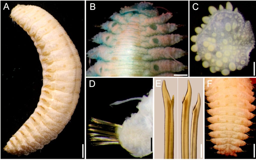
Parapodia short, 1/4 as long as body width; dorsally with transverse rows of globular tubercles along notopodia, remaining surface with papillae, ventrally with transverse pleats and scattered papillae. Notopodia reduced, acicular lobe small, with an apical papilla. Neuropodia truncate, dorsally furrowed, prechaetal lobe slightly larger than postchaetal one, with some distal papillae.
Cirrigerous segments with cylindrical, thick, short cirrophores, cirrostyles smooth, long, almost smooth, reaching the neuropodial tip (Fig. 11D). Nephridial papillae low, blunt, from chaetiger 12, continued to chaetiger 25, progressively larger.
Neurochaetae amber color. Most body segments with 2-3 notochaetae, curved, marginally denticulate. Neurochaetae decreasing in size and width ventrally, most with 2 accessory teeth, on lower position (Fig. 11E).
Posterior region tapered, truncate; pygidium with anus terminal, anal cirri lost (Fig. 11F).
Taxonomic summary
Type material. Arabian Sea. Holotype (SMF 136089, Socotra Island, Sta. 726, 8-10 m, 9 Apr. 2000, T. Wehe, coll.
Distribution. Known only from Socotra Island, Arabian Sea, and from Saya de Malha Bank, Indian Ocean; in subtidal substrates (8-26 m).
Etymology. The specific epithet is after Dr. Thomas Wehe, in recognition of his relevant publications on scaleworms, and especially because he collected the holotype.
Additional material: Indian Ocean, Saya de Malha Bank.One specimen (MNHN IA 2017-4879), Saya Expedition, RV Agulhas II, Sta. YS08 (09°41.9’ S, 60°51’ E), 26 m, 8 Nov. 2022, S. Hourdez, coll. (complete, bent ventrally, with ill-defined transverse bands in elytrigerous segments; first elytra pair markedly larger than following ones, barely covering prostomial sides; pharynx everted, 4 mm long, with 10 pairs of terminal papillae; right parapodium of chaetiger 15 removed for observation; neurochaetae with a single accessory denticle (rarely double); body 19 mm long, 5 mm wide, 26 chaetigers).
One specimen (MNHN 2021-727), Saya Expedition, RV Agulhas II, Sta. YS08 (16°50’ S, 59°31.3’ E), 17 m, 20 Nov. 2022, S. Hourdez, coll. (complete, bent ventrally with ill-defined transverse bands in elytrigerous segments; first elytra pair markedly larger than following ones, barely covering prostomial sides; left parapodia of chaetigers 16-19 removed for molecular studies; body 23 mm long, 6.5 mm wide, 26 chaetigers).
Remarks
Hermenia wehei sp. nov. belongs to the group of species (H. verruculosa, H. treadwelli) having only the first pair of elytra markedly larger than the following ones. However, H. wehei separates from the other species regarding differences in the first elytra, the development of middorsal tubercles, and in neurochaetal tips. Thus, H. wehei has the first elytra with macrotubercles clearly projected beyond the margin (against barely projected), medium-sized middorsal tubercles (against having larger ones middorsally), and its neurochaetae are bidentate or tridentate (against only bidentate in the other species).
Key to species of Hermenia Grube & Örsted in Grube, 1856
1 First 2-3 anterior pairs of elytra markedly larger than posterior ones; neurochaetae of median segments with 2 accessory teeth
………………………………………………………………………………2
– Only first pair of elytra markedly larger than posterior ones; neurochaetae of median segments with 1 accessory denticle, rarely with 2 accessory teeth
………………………………………………………………………………5
2 (1) Dorsum whitish, papillate or barely tuberculate; elytral macrotubercles globular, basally swollen or L-shaped (inner projection smaller)
………………………………………………………………………………3
– Dorsum grayish, clearly tuberculate; tubercles arranged in transverse series; elytral macrotubercles globular, no L-shaped
………………………………………………………………………………4
3 (2) Median and posterior elytra covering up to half of adjacent segments, elytra round, last one slightly larger than previous one
………………………………………………………………………………H. acantholepis (Grube, 1876) Philippines
– Median and posterior elytra barely covering adjacent segments, elytra oval to circular, last elytra as large as previous one
………………………………………………………………………………H. mezianei sp. nov. Vietnam
4 (2) Dorsum with rows of globular tubercles, each with blackish core; median and posterior elytra with black macrotubercles
………………………………………………………………………………H. neoverruculosa Pettibone, 1975 Cargados Carajos, Indian Ocean
– Dorsum with rows of depressed tubercles, each with pale core; median and posterior elytra with pale and brownish macrotubercles
………………………………………………………………………………H. chuarae sp. nov. Indonesia
5 (1) Neurochaetae with a single accessory tooth; middorsal surface with large globular tubercles; first left elytron with macrotubercles barely projected beyond margin
………………………………………………………………………………6
– Neurochaetae with 1-2 accessory teeth; middorsal surface without large globular tubercles; first left elytron with macrotubercles distinctly projected beyond margin
………………………………………………………………………………H. wehei sp. nov. Arabian Sea
6 (5) Segment 2 with nuchal lappet over prostomium; dorsal cirrostyle of median segments with swollen area brownish (fresh specimens with chaetigers 1-5 almost completely white, or with a large white inverted triangular spot over the dorsum of the chaetigers 3-5)
………………………………………………………………………………H. treadwelli sp. nov. Grand Caribbean Sea
– Segment 2 without nuchal lappet over prostomium; dorsal cirrostyle of median segments with swollen area whitish (fresh specimens with a middorsal white rectangular spot, or dorsum completely dark along chaetigers 5-6, sometimes separated by brownish area into 3 spots)
………………………………………………………………………………H. verruculosa Grube & Örsted in Grube, 1856 U.S. Virgin Islands, Caribbean Sea
Parahermenia gen. nov.
http://zoobank.org/urn:lsid:zoobank.org:act:5604018E-9BC0-4D3C-908F-1E355BAEFE7A
Diagnosis. Lepidonotinae with short body; integument papillate, venter papillate. Body with 26 segments, 12 pairs of elytra on segments 2, 4, 5, 7, 9, 11, 13, 15, 17, 19, 21, 23. Prostomium bilobed, with 2 pairs of eyes. Elytra with globular macrotubercles and microtubercles, abundant papillae, fimbriae very long; elytra of similar size along body, overlapping laterally, not dorsally. Tentacular segment with few notochaetae and bulbous facial tubercle. Parapodia subbiramous, notopodia small, neuropodia large. Notochaetae long, slender, finely spinous. Neurochaetae stout, falcate, with 1-2 large accessory teeth. Dorsal cirri with cirrophores cylindrical, cirrostyles short. Ventral cirri short, subulate. Pharynx with 2 pairs of jaws and 9 pairs of marginal papillae. Nephridial papillae short, cylindrical, from chaetigers 6-8.
Taxonomic summary
Type species. Lepidonotus hermenioides Amoureux, 1974.
Distribution. Parahermenia includes 2 species found in shallow water sediments, 1 from Madagascar, the other from the Philippines.
Etymology. Parahermenia is made by combining the stem genus name Hermenia with the Greek prefix para-, meaning “besides, nearby” (Brown 1954: 587), and this new name indicates the affinities to the older genus group name. Gender: Feminine.
Remarks
Pettibone (1977:40) noted that there are 3 genera with long filiform papillae on the distal end of neuropodia. She proposed 2 new genera, Lepidonopsis Pettibone, 1977 and Parahalosydnopsis Pettibone, 1977, which, together with Halosydnopsis Uschakov & Wu, 1959, were the only genera provided with filiform papillae. The number of pairs of elytra and neurochaetal tips separates these 3 genera because Lepidonopsis has 12 pairs and bidentate neurochaetae, Halosydnopsis has 17 and unidentate neurochaetae, and Parahalosydnopsis has about 30 pairs and unidentate neurochaetae. These 3 genera have small denticles in series along the pectinate area.
Lepidonotus hermenioides does not belong in Lepidonopsis although it has 12 pairs of elytra, because each elytron is provided with very long fimbria, only 2 macrotubercles in the insertion area and the elytra do not overlaped dorsally, whereas in Lepidonopsis the elytra overlap covering the body, have short fimbriae and different types of microtubercles (Salazar-Silva & Carrera-Parra, 2014). On the other hand, L. hermenioides does not fall within Hermenia despite sharing a papillate integument, and neurochaetae with 1-2 accessory teeth. The main differences are in the elytra. In L. hermenioides elytra are of similar size along the body, overlapping laterally but not dorsally, and their margin has abundant long fimbriae, whereas in the species of Hermenia median and posterior segments have elytra that do not overlap laterally or dorsally, and fimbriae are minute.
Amoureux (1974) avoided proposing a new genus because he only had a single specimen, and it was regarded as a very small juvenile. He might have suspected some ontogenetic modifications that would complicate separating the new group. We agree this and the new species described below include small specimens; however, after the study of many specimens of different size, we do not find evidence that elytra would be so drastically modified such that they would become progressively smaller during growth, or that the elytral margins would be modified from having very long fimbriae to becoming progressively reduced to become minute.
Parahermenia hermenioidea (Amoureux, 1974) comb. nov.
(Fig. 12)
Lepidonotus hermenioides Amoureux, 1974: 131, Fig. 1.
Diagnosis. Parahermenia with body papillate, elytra with long filamentous papillae, without macrotubercles or spines, margin fimbriate; neurochaetae with 2-3 accessory large teeth.
Description. Holotype (MNHN POLY TYPE 1275) complete, brownish, with abundant papillae along body (Fig. 12A); pharynx fully exposed; elytra paler with long fimbriae, and filaments on elytral surface; first pair of elytra on site, right elytra 10 and 12 on site; right parapodia of chaetigers 10, 12, 14, and left parapodia of chaetigers 13 and 14 previously removed (1 elytron and 1 parapodium in container). Body depressed, wider anteriorly, 3.5 mm long (pharynx 0.8 mm long), 1.2 mm wide (without chaetae), 23 chaetigers.
Prostomium oval, as long as wide; only left lateral antenna, ceratostyle on site, short, all other lost (Fig. 12B); median antenna ceratophore about twice wider than laterals. Palps lost. Eyes indistinct. Pharynx cylindrical, grayish, with 9 pairs of marginal papillae.
Facial tubercle globular, small. Tentacular segment indistinct dorsally; second segment chaetiger without nuchal lappet, dorsum without tubercles; tentacular cirri present on left side, 4-5 times longer than left antenna, subdistally swollen, with 4-5 chaetae.
Ventral cirri of chaetiger 2 are about 3-4 times longer than the following ones, surpassing neurochaetal tips. Nephridial lobes barely developed, not visible.
Elytra oval, with 2 globular macrotubercles in the insertion area, each with small conical papillae; microtubercles conical over elytral surface, and long filaments on surface, margin with long fimbriae, filaments 1/2-1/3 elytral length (Fig. 12C).
Parapodia biramous. Notopodia reduced, low round lobes. Dorsal cirri resembling tentacular cirri, barely swollen subdistally. Notochaetae thin, with a single series of fine denticles (Fig. 12D).
Neuropodia larger, prechaetal and postchaetal lobes blunt, papillate. Neurochaetae barely swollen subdistally, unidentate, with 2-3 large subdistal accessory teeth (Fig. 12E).
Posterior region truncate; pygidum with anus terminal, anal cirri tapered, resembling dorsal cirri.
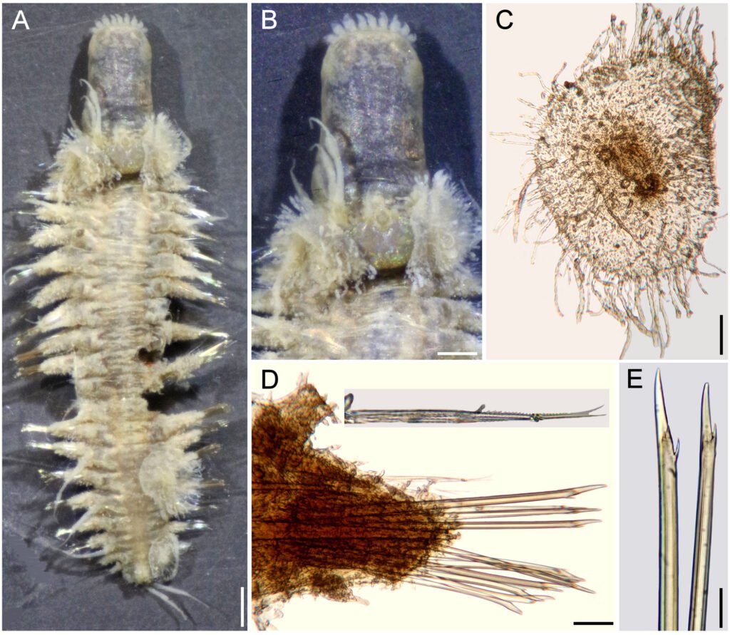
Taxonomic summary
Type material. Madagascar. Holotype of Lepidonotus hermenioides Amoureux, 1974 (MNHN POLY TYPE 1275), Nosy Tanikely, Madagascar, comb-dredge (faubertage) 1, 15 m, 6 Apr. 1960, G. Cherbonnier, leg.
Distribution. Only known from a single locality in Madagascar, in shallow rocky bottoms.
Remarks
Parahermenia hermenioidea (Amoureux, 1974) comb. nov. needed an alteration of the specific name for matching the genus gender. This is regarded as an adjective and, after Brown (1954: 483), the suffix –oid, –oides, –odes, –oideus, –a, –um, are derived from the Greek suffix –eides meaning “like, resembling, having the form of”. He also indicated that –oideus, –a, –um have their gender indicated by the adjectival endings –us, –a, –um.
Amoureux (1974) noted that the neurochaetae of Lepidonotus hermenioides resembles those present in Hermenia, and this explains the specific name. The generic affinities are problematic because L. hermenioides does not match Hermenia by having median and posterior elytra larger, with long fimbriae and long papillae along its surface, instead of large globular macro- and microtubercles and short fimbriae, as revised Pettibone (1975).
Parahermenia piotrowskiae sp. nov.
(Fig. 13)
http://zoobank.org/urn:lsid:zoobank.org:808A56BB-18
7E-4E60-97D9-DF4308793F2E
Diagnosis. Parahermenia with body papillate, elytra with globular macrotubercles and a single spine, and few filamentous papillae, margin fimbriate; neurochaetae with 2-3 accessory large teeth.
Description. Holotype (CAS 217917), complete, markedly bent ventrally, with abundant papillae along body; dorsum and vente white, first and last pairs of elytra whitish, first with 3 colorless macrotubercles, arranged in a triangle, last elytra with a single colorless globular macrotubercle; other elytra with globular brownish macrotubercles centrally, and long filamentous fimbriae. Second pair of elytra with 3 large globular central macrotubercles, arranged in a triangle (Fig. 13A), following elytra with smaller macrotubercles, arranged in an oblique row or a triangle (Fig. 13B). Some left median and posterior elytra detached; right elytron 6 and left parapodium of chaetiger 12 removed for observation (all kept in container). Body depressed, slightly tapered posteriorly, 6 mm long, 2 mm wide, 26 chaetigers.
Prostomium hexagonal, about as long as wide; median ceratophore 2 times as large and long as laterals, median ceratostyle lost; lateral ceratostyles tapered, subdistally swollen, 1/5 as long as palps, with reddish bands below and over swollen area, tips reddish. Palps papillate, with 2 longitudinal lateral reddish bands, middorsal area pale, with a subdistal reddish band, tips darker. Eyes black, of similar size, anterior eyes in wider prostomial area, posterior ones close to posterior margin.
Facial tubercle globular, small. Tentacular segment indistinct dorsally; second chaetiger without nuchal lappet, dorsum with transverse reddish bands, without tubercles; tentacular cirri resembling lateral antennae in pigmentation, slightly shorter than palps, chaetae not seen.
Ventral cirri of chaetiger 2 lost. Nephridial lobes not seen. Median elytra oval, overlapping laterally, not dorsally. Each with 2-3 large, central reddish or brownish globular macrotubercles, some with 4 (Fig. 13C), others with 2-3 macrotubercles, a single large falcate spine external to globular macrotubercles, and sparse papillae, most short (about as long as wide), a few 4-6 times longer than wide; fimbriae with cylindrical filaments, some distally swollen, 1/10-1/7 elytral length.
Parapodia biramous (Fig. 13D). Dorsal cirri resembling tentacular cirri, barely swollen subdistally, with brownish bands before and after a swollen dark area (Fig. 13D), ceratostyle with small papillae. Notochaetae thin, with a single series of fine denticles (Fig. 13D, inset below).
Neuropodia larger, prechaetal and postchaetal lobes blunt, papillate. Neurochaetae barely swollen subdistally, unidentate, with 2 large subdistal teeth (Fig. 13E).
Posterior region truncate; pygidium with anus terminal (Fig. 13F), anal cirri resembling dorsal cirri.
Taxonomic summary
Type material. Philippine Islands. Holotype (CAS 217917), Verde Island Passage Expedition 2016, Luzon Island, Batangas Province, Tingloy, Maricaban Island, Devil’s Point (13.65°N, 120.84°E), coral rubble, 40 m, 20 Apr. 2016, C. Piotrowski, coll.
Distribution. Only known from a subtidal locality (40 m) in Luzon Island, Philippines.
Etymology. This species is being named after M.Sc. Christina N. Piotrowski, Collection Manager of the Invertebrate Zoology collections in the California Academy of Sciences, in recognition of her support of our research activities, and because of her sampling efforts in many tropical localities of the world, especially because she collected the holotype.
Remarks
Parahermenia piotrowskiae sp. nov. resembles P. hermenioidea, the other only known species in the genus, because both have small bodies, and their elytra have long filamentous fimbriae. Their main differences are in the elytral ornamentation. In P. piotrowskiae elytra have globular, usually pigmented macrotubercles and a single spine, sparse filamentous papillae, and the fimbriae filaments are short, 1/10-1/7 as long as elytral length, whereas in P. hermenioidea the macrotubercles are markedly smaller, and there are no large spines, its filamentous papillae are long and abundant, and the fimbriae filaments are long, 1/2-1/3 of elytral length.
Key to species of Parahermenia gen. nov.
1 Median segments with elytral surface provided with large, reddish or brownish macrotubercles, a single large spine, papillation sparse; elytral fimbriae short (1/10-1/7 elytral length)
………………………………………………………………………………P. piotrowskiae sp. nov. Philippines
– Median segments with elytral surface provided with small, pale macrotubercles, without spines, papillation abundant; elytral fimbriae long (1/2-1/3 elytral length)
……………………………………………………………………………… P. hermenioidea (Amoureux, 1974) comb. nov. Madagascar.
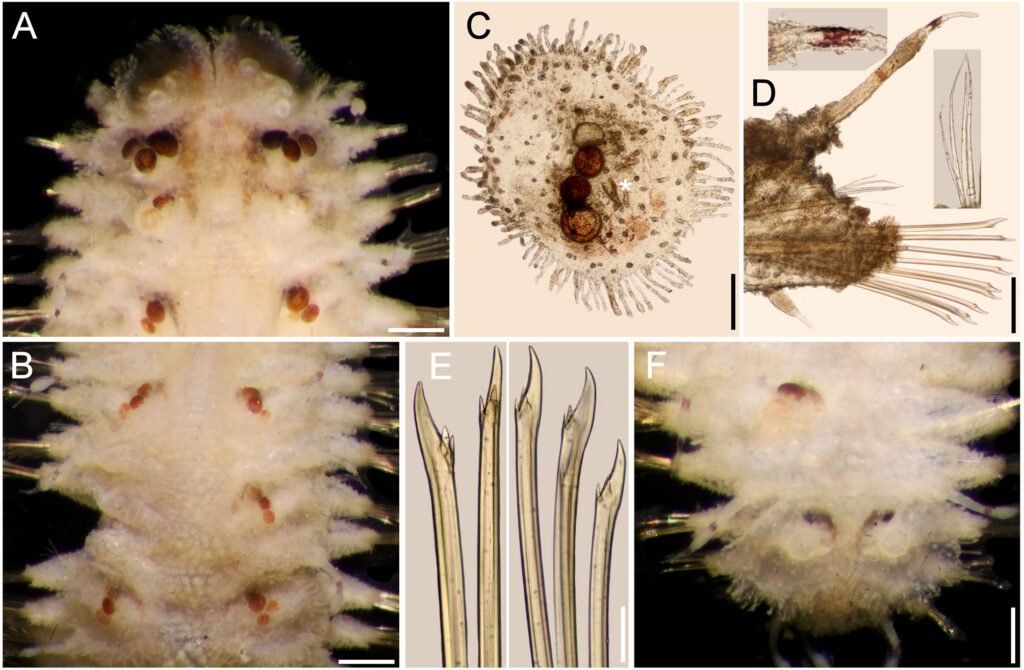
Discussion
The taxonomy of polynoid scaleworms has relied on morphological characters, such as the arrangement of cephalic appendages (subfamilies), and the features of the elytral and parapodial structures, including chaetae. Among Lepidonotinae, the traditional approach has been to use the number of pairs of elytra and other parapodial features for separating similar genera. In the group of lepidonotin genera provided with 12 pairs of elytra, the distinguishing features include the presence of some parapodial features (branchiae, pseudelytra) or types of chaetae. We have confirmed the distinguishing features of Hermenia such as the presence of reduced elytra along most body segments, and that neurochaetae have subdistal smooth regions, as opposed to most other genera having spinulose regions, and tips bi- or tridentate, opposed to being uni- or bidentate.
We have also refined the use of some distinguishing features for separating similar Hermenia species, and for newly describing other ones. They include the modifications of the nuchal lappet (distinctive, or indistinct), body integument (tuberculate, papillate, or both) and pigmentation, shape of elytra (mostly circular, some oval, wider than long), elytral size along body (similar to body end, or last pair larger than median ones), type of macrotubercles (most ovoid, a few basally swollen), and tips of neurochaetae (bi- or tridentate). Hermenia now includes 3 previously known species: H. verruculosa, described from the Caribbean Sea (type species), H. acantholepis, described from Philippines, and H. neoverruculoa, from Republic of Mauritius, and 4 new species: H. chuarae sp. nov. from Indonesia, H. mezianei sp. nov. from Vietnam, H. treadwelli sp. nov. from the Grand Caribbean, and H. wehei sp. nov. from the Arabian Sea and Indian Ocean.
Two other species, one already described, and another undescribed, resembled Hermenia species by having body papillate and neurochaetae subdistally smooth, but differed by having larger elytra overlapping laterally along body (restricted to a few anterior pairs in Hermenia), and elytra provided with long fimbria (short in Hermenia) and a few macrotubercles (very abundant in Hermenia). We proposed Parahermenia gen. nov. for these 2 species and separated them after the size of elytral fimbriae and number of macrotubercles. The new genus contains P. hermenioidea comb. nov. from Madagascar, and P. piotrowskiae sp. nov. from the Philippines. An interesting fact that no species of Hermenia or Parahermenia have been found along the Eastern Pacific or Western African coasts.
Acknowledgments
To Christina Piotrowski (CAS), Danny Eibye-Jacobsen and the late Mary Petersen (ZMUC), Leslie Harris (LACM), Marie-Louise Tritz and Ekin Tilic (SMF), Miranda Lowe and Emma Sherlock (BMNH), the late Nancy Voss and María Criales (UMML), Gisela Wegener and Angelika Brandt (ZMH), Fredrik Pleijel, Tarik Meziane, Laure Corbari and Stéphane Hourdez (MNHN), Gustav Paulay and Amanda Bemis (UF), kindly allowed us to study part of their collections. The then-known Consejo Nacional de Ciencia y Tecnología, México, funded the project Poliquetos del Gran Caribe (Conacyt 32529T), and provided a PhD scholarship to the first author (Conacyt 94497). The warm support by the late Kristian Fauchald and Len Hirsch, as well as Leslie Harris and David Ocker, Laure Corbari and Tarik Meziane, allowed us to make research visits to study their magnificent collections. Emilia González and Luis F. Carrera-Parra took care of the ECOSUR Reference Collection.
References
Amoureux, L. (1974). Annélides polychètes de Madagascar recueillies par G. Cherbonnier en 1960. Bulletin du Museum National d Histoire Naturelle, Paris, série 3, Zoologie, 217, 425–462.
Baird, W. (1865). Contributios towards a monograph of the species of Annelides belonging to the Aphroditacea, containing a list of the know species, and a description of some new species contained in the National Collection of the British Museum. Journal of the Linnean Society, Zoology, 8, 172–202. https://doi.org/10.1111/j.1096-3642.1865.tb02438.x
Bellan, G. (1964). Résultats scientifiques des campagnes de la Calypso dans l’Atlantique. Annélides polychetes. Annales de l’Institute Océanographique, 41, 301–314.
Ben-Eliahu, M. N. (1975). Polychaete cryptofauna from rims of similar intertidal vermetid reefs on the Mediterranean coast of Israel and in the Gulf of Elat: Sabellidae (Polychaeta Sedentaria). Israel Journal of Zoology, 24, 54–70. https://doi.org/10.1080/00212210.1975.10688411
Brown, R. W. (1954). Composition of scientific words: a manual of methods and a lexicon of materials for the practice of logotechnics. Baltimore: George W. King.
Chuar, C. H., Hadiyanto, H., & Lee, Y. L. (2021). Annotated checklist of polychaetes from deeper waters of the Sunda Strait and eastern Indian Ocean off southwest Java, Indonesia. Raffles Bulletin of Zoology, 36 (Supplement), 47–77. https://doi.org/10.26107/RBZ-2021-0030
Dawydoff, C. (1952). Contribution a l’étude des invertébrés de la faune marine benthique de l’Indochine. Bulletin Biologique de la France et de la Belgique, 37 (Supplement), 1–158.
Devaney, D. M. (1974). Shallow-water echinoderms from British Honduras, with a description of a new species of Ophiocoma (Ophiuroidea). Bulletin of Marine Science, 24, 122–164.
Ebbs, N. K. (1966). The coral-inhabiting polychaetes of the northern Florida reef tract, 1. Aphroditidae, Polynoidae, Amphinomidae, Eunicidae, and Lysaretidae. Bulletin of Marine Science, 16, 485–555.
Fauchald, K. (1977). The polychaeta worms: Definitions and keys to the orders, families and genera. Natural History Museum of Los Angeles County, Science Series, 28, 1–188.
Fauvel, P. (1922). Annélides polychètes de l’Archipel Hontman Abrolhos (Australie Occidentale) recueillies par M. le Prof. W.J. Dakin, F.L.S. Journal of the Linnean
Society,Zoology,34, 487–500. https://doi.org/10.1111/j.1096-3642.1922.tb01843.x
Fauvel, P. (1932a). Annelida Polychaeta of the Indian Museum, Calcutta. Memoirs of the Indian Museum, 12, 1–262.
Fauvel, P. (1932b). Mission Robert Ph. Dollfus en Égypte (Décembre 1927 – Mars 1929). Résumé analytique sur les polychètes. Bulletin de I institut d Égypte, 15, 131–144. https://doi.org/10.3406/bie.1932.3260
Fauvel, P. (1933). Mission Robert Ph. Dollfus en Égypte (Décembre 1927 – Mars 1929). Annélides polychètes. Bulletin de l’Institut d’Égypte, 21, 31–83.
Fauvel, P. (1935). Annélides polychètes de l’Annam. Memorie de lla Pontificia Accademia Romana dei Nuovi Lincei, série 3, 2, 279–354.
Fauvel, P. (1939). Annélides polychètes de l’Indochine recueillies par M. C. Dawydoff. Comment Pontificale Academie des Sciences, Civ Vaticana, 3, 243–368.
Fauvel, P. (1947). Faune de l’Empire Français, 8. Annélides polychètes de Nouvelle-Calédonie et des Iles Gambier. Paris: Office de la Recherche Scientifique Coloniale.
Fauvel, P. (1953a). The fauna of India including Pakiastan, Ceylon, Burma and Malaya: Annelida Polychaeta. Allhabad: Indian Press.
Fauvel, P. (1953b). Annélides polychétes de la Croisiére du Président Theodore Tissier aux Antilles. Bulletin de l’Institut Océanographique, Monaco, 1033, 1–23.
Grube, E. (1850). Die Familien der Anneliden. Archiv für Naturgeschichte, Berlin, 16, 249–364.
Grube, E. (1851). Uebersicht der Annelidengattungen und Arten zu ihrer vorläufigen Uterschidung. In Die Familien der Anneliden mit Angabe ihrer Gattungen und Arten. Ein systematischer Versuch (pp. 117–164). Berlin: Nicolai’schen Buchhandlung.
Grube, A. E. (1856). Annulata Örstediana Enumeratio Annulatorum, quae in itinere per Indiam occidentalem et Americam centralem annis 1845-1848 suscepto legit cl. A. S. Örsted, adjectis speciebus nonnullis a cl. H. Kröyer in itinere ad Americam meridionalem collectis. Havniae Part, 1, 44 – 62.
Grube, E. (1878). Annulata Semperiana. Memoires de l’Academie Imperiale des Sciences de St. Petersbourg, série 7, 25, 1–300.
Hanley, J. R., & Burke, M. (1991). Polychaeta Polynoidae: scaleworms of the Chesterfield Island and Fairway Reef, Coral Sea. In A. Crosnier (Ed.), Resultats des campagnes Musorstom 8 (pp. 9–82). Paris: Mémoires du Muséum National d’Histoire Naturelle.
Hartman, O. (1939). The polychaetous annelids collected on the Presidential Cruise of 1938. Smithsonian Miscellaneous Collections, 98, 1–22.
Herdman, W. A., & Hornell, J. (1903). Narrative with an outline of the investigation and details of the stations where observations were made. Report to the Government of Ceylon on the pearl oyster fisheries of the Gulf of Manaar, 1, 17–98.
Horst, R. (1917). Polychaeta Errantia of the Siboga-Expedition, 2. Aphroditidae and Chrysopetalidae. Siboga-Expeditie Monographie, Leyden, 24b, 1–140.
Horst, R. (1922). On some polychaetous annelids from Curaçao. Bijdragen tot de Dierkunde, 22, 193–201.
Imajima, M. (1997). Polychaetous annelids from Sagami Bay and Sagami Sea collected by the Emperor Showa of Japan and deposited at the Showa Memorial Institute, National Science Museum, Tokyo. Families Polynoidae and Acoetidae. National Science Museum, Tokyo Monographs, 13, 1–130.
Kinberg, J. G. H. (1856). Nya slägten och arter af Annelider. Animalia Annulata nova 1. Minus rite cognita recensuit. Öfversigt af Kongliga Vetenskaps-akademiens forhan-
dlingar, 12, 9–10, 381–388.
Monro, C. C. A. (1924). On the Polychaeta collected by H.M.S. ‘Alert’, 1881-1882. Families Polynoidae, Sigalionidae, and Eunicidae. Journal of the Linnean Society of London, Zoology, 36, 37–64. https://doi.org/10.1111/j.1096-3642.1924.tb02207.x
Monro, C. C. A. (1939). On some tropical polychaetes in the British Museum mostly collected by Dr. C. Crossland at Zanzibar, Tahiti, and the Marquesas, 1. Families Amphinomidae to Phyllodocidae. Annals and Magazine of Natural History, series 11, 4, 161–184.
O’Hara, T. D., Hugall, A. F., Cisternas, P. A., Boissin, E., Bribiesca-Contreras, G., Sellanes, J. et al. (2019). Phylogenomics, life history and morphological evolution of ophiocomid brittlestars. Molecular Phylogenetics and Evolution, 130, 67–80. https://doi.org/10.1016/j.ympev.2018.10.003
Pettibone, M. H. (1975). Review of the genus Hermenia, with a description of a new species (Polychaeta: Polynoidae: Lepidonotinae). Proceedings of the Biological Society of Washington, 88, 233–248.
Pettibone, M. H. (1977). Review of Halosydnopsis and related genera (Polychaeta: Polynoidae: Lepidonotinae). In D. J. Reish, & K. Fauchald (Ed.), Essays on polychaetous annelids in memory of Dr. Olga Hartman (pp. 39–62). The Allan Hancock Foundation, University of Southern California. Los Angeles.
Pettibone, M. H. (1993). Scaled polychaetes (Polynoidae) associated with ophiuroids and other invertebrates and review of species referred to Malmgrenia McIntosh and replaced by Malmgreniella Hartman, with descriptions of new taxa. Smithsonian Contributions to Zoology, 538, 1–92.
Pruvot, G. (1930). Annélides polychètes de Nouvelle-Calédonie recueillies par M. François. Archives de Zoologie Expérimentale et Générale, Paris, 70, 1–94.
Salazar-Silva, P., & Carrera-Parra, L. F. (2014). Revision of Lepidonopsis humilis (Augener, 1922) and description of L. barnichae sp nov (Annelida: Polychaeta: Polynoidae) based upon morphological and molecular characters. Zootaxa, 3790, 555–566. https://doi.org/10.11646/zootaxa.3790.4.4
Salazar-Vallejo, S. I. (1996). Lista de especies y bibliografía de poliquetos (Polychaeta) del Gran Caribe. Anales del Instituto de Biología UNAM, serie Zoología, 67, 11–50.
Salazar-Vallejo, S. I., & Eibye-Jacobsen, D. (2012). Annulata örstediana: Publication dates, composition and annotated taxonomic list, with some comments on Hemipodus (Polychaeta: Glyceridae). Revista de Biologia Tropical, 60, 1391–1402.
Seidler, H. J. (1923). Über neue und wenig bekannt Polychäten. Zoologischen. Anzeiger, Leipzig, 56, 254–264.
Seidler, H. J. (1924). Beitrage zur Kenntnis der Polynoiden, 1. Archiv für Naturgeschichte, 89A, 1–217.
Treadwell, A. L. (1911). Polychaetous annelids, from the Dry Tortugas, Florida. Bulletin of the American Museum of Natural History, 30, 1–12.
Wehe, T. (2006). Revision of the scale worms (Polychaeta: Aphroditoidea) occurring in the seas surrounding the Arabian Peninsula. Part 1. Polynoidae. Fauna Arabia, 22, 23–197.

Lo pasado, pasado: actualización taxonómica y distribución geográfica de la flora vascular de la Estación de Biología Tropical Los Tuxtlas, Veracruz, México
What’s done is done: taxonomic update and geographical distribution of the vascular flora of the Los Tuxtlas Tropical Biology Station, Veracruz, Mexico
Guillermo Ibarra-Manríquez *, Guadalupe Cornejo-Tenorio y Santiago Sinaca-Colín
Universidad Nacional Autónoma de México, Instituto de Investigaciones en Ecosistemas y Sustentabilidad, Antigua carretera a Pátzcuaro Núm. 8701, 58190 Morelia, Michoacán, México
*Autor para correspondencia: gibarra@iies.unam.mx (G. Ibarra-Manríquez)
Recibido: 21 julio 2025; aceptado: 10 octubre 2025
Resumen
El objetivo principal del presente trabajo es actualizar la nomenclatura y el inventario de las especies registradas en la Estación de Biología Tropical Los Tuxtlas (ELT), localizada en el estado de Veracruz, con base en la consulta de literatura florístico-taxonómica, ejemplares de herbario, bases de datos electrónicas y taxónomos. Se registran 934 especies, 571 géneros y 139 familias. Las 20 familias con mayor número de especies abarcan 58.8% de la flora, destacando Orchidaceae (108 especies), Asteraceae (61) y Fabaceae (58); los géneros más relevantes fueron Epidendrum (16), Piper (14) y Ficus (10). Un total de 48 familias (34.5%) y 410 géneros (71.8%) están representados por una especie. Las formas de crecimiento más frecuentes son las hierbas (453 especies, 48.5%) y árboles (259, 27.7%). Noventa y tres especies (10%) son endémicas de México. Las especies de la ELT que se comparten exclusivamente con Centroamérica son las más frecuentes (29.8%), seguidas por las que se registran conjuntamente en Centroamérica, Antillas y Sudamérica (23.2%). Se enfatiza la importancia de continuar con el inventario de esta reserva ubicada en una de las regiones con mayor tasa de deforestación en México.
Palabras clave: Endemismo; Forma de crecimiento; Hábito; Selva alta perennifolia
Abstract
The main objective of this work is to update the nomenclature and inventory of the flora of the Los Tuxtlas Tropical Biology Station, located in Veracruz State, based on floristic-taxonomic literature, herbarium specimens, electronic databases, and support of taxonomists. We registered 934 species, 571 genera, and 139 families. The 20 families with the greatest number of species comprise 58.8% of the flora, highlighting Orchidaceae (108 species), Asteraceae (61), and Fabaceae (58); the most specious genera were Epidendrum (16), Piper (12), and Ficus (10). Forty-eight families (34.5%) and 410 genera (71.8%) are represented by one species. The most common growth forms were herbs (453, 48.5%) and trees (259, 27.7%). Ninety-three species (10%) are endemic to Mexico, and 29.8% of the species are shared exclusively with Central America, followed by the area encompassing Central America, Antilles, and South America (23.2%). The importance of maintaining the inventory of this conservation area in one of Mexico’s regions with the highest rates of deforestation, is emphasized.
Key words: Endemism; Growth form; Life form; Tropical rain forest
Introducción
La región de Los Tuxtlas, localizada en el estado de Veracruz, forma parte de una de las áreas con mayor número de especies del bioma bosque tropical húmedo en México (Villaseñor, 2016) y fue incluida en la provincia biogeográfica de la Costa del Golfo de México por Rzedowski (1978), perteneciente al Reino Neotropical, lo que concuerda con la delimitación de este reino propuesta por Liu et al. (2023). En esta región se decretó, en 1998, la Reserva de la Biosfera Los Tuxtlas, con una extensión de 155,122-46-90 ha (Conanp, 2006). El establecimiento de esta reserva concuerda con su designación como una de las áreas prioritarias más importantes para la conservación de los bosques húmedos de México (Villaseñor et al., 2003). En la zona núcleo Volcán San Martín Tuxtla de esta reserva de la biosfera, se asienta la Estación de Biología Tropical Los Tuxtlas (ELT), perteneciente a la Universidad Nacional Autónoma de México.
De acuerdo con Reynoso et al. (2017), la ELT tiene como áreas de investigación fundamentales el inventario de las especies que protege y estudios sobre la ecología y restauración de la selva tropical húmeda de la región de Los Tuxtlas. Ambas áreas de investigación requieren conocimiento confiable sobre la identidad taxonómica de las especies que conforman su flora. En particular, la primera de ellas no ha perdido vigencia, puesto que los inventarios florísticos son un componente fundamental de agendas de investigación nacionales e internacionales (e.g., Daly et al., 2012; Villaseñor y Meave, 2022), ya que sus resultados permiten realizar distintos tipos de análisis para la obtención de patrones biogeográficos, ecológicos y evolutivos de la biodiversidad (Antonelli et al., 2023; Raven et al., 2020; Sarukhán et al., 2015; Ulloa et al., 2017; Villaseñor y Meave, 2022; Villaseñor y Ortiz, 2014).
Con base en el material de colectores botánicos pioneros como Juan Ismael Calzada, Refugio Cedillo Trigos, Guadalupe Martínez Calderón, Marino Rosas R. y Ángel Villegas Herrera, así como en el trabajo florístico, iniciado en febrero de 1982 para establecer un herbario de referencia para la ELT, Ibarra-Manríquez y Sinaca (1987) publicaron el primer listado de plantas de esta área de conservación. Posteriormente, con el objetivo de aportar datos más detallados de cada especie —e.g., nombre común, forma de crecimiento, fenología reproductiva, usos—, estos autores publicaron una lista comentada (Ibarra-Manríquez y Sinaca, 1995, 1996a, b), en la que se reportaron 940 especies y 543 géneros, agrupados en 137 familias. Un análisis de los usos que para el ser humano tiene este contingente florístico se encuentra en Ibarra-Manríquez, Ricker et al. (1997), así como de su potencial para actividades de restauración regional (Ibarra-Manríquez 2017).
Otras publicaciones que pueden citarse relacionadas con el conocimiento florístico de la ELT son las diagnosis de especies de palmas y trepadoras (Campos et al., 2004; Ibarra-Manríquez, 1988), así como de los frutos y semillas de cerca de 350 especies (Ibarra-Manríquez et al., 2015; Sánchez-Garfías et al., 1991). Más recientemente, Cornejo-Tenorio et al. (2019) publicaron una guía ilustrada que incluye 464 especies con diversas formas de crecimiento. Para toda la región de Los Tuxtlas, existe un manual de determinación de especies de árboles (Vázquez et al., 2010), así como el trabajo de Villaseñor et al. (2018), en el que se analizan distintos aspectos de la flora y que incluye una lista de 2,548 especies.
En el presente siglo, han ocurrido avances sustanciales en el conocimiento florístico y taxonómico de las plantas neotropicales. Por ejemplo, hace todavía un par de décadas habría sido difícil pensar que se contaría con un listado de la flora mexicana (Villaseñor, 2016) y, menos probable aún, con un inventario florístico para todo el continente americano (Ulloa et al., 2017). Estos progresos han sido impulsados, entre otros aspectos, por el desarrollo de bases electrónicas que manejan un gran cúmulo de datos (e.g., POWO, 2025; Tropicos, 2025), en combinación con la conformación del Angiosperm Phylogeny Group, el cual se ha abocado a la elaboración de un sistema de clasificación que refleje, cada vez con mayor precisión, las relaciones de parentesco entre los diferentes taxones de las plantas vasculares de todo el mundo (APG IV, 2016).
Como se describe en el párrafo previo, la lista aportada por Ibarra-Manríquez y Sinaca (1995, 1996a, b), la más detallada para toda la flora de la ELT, requiere una revisión nomenclatural, lo cual fue sugerido previamente por Ibarra-Manríquez (2017). En consecuencia, el presente estudio tiene como objetivos principales: 1) actualizar la nomenclatura taxonómica de las especies registradas en esta área de conservación, 2) adicionar a su inventario las especies descritas desde 1997 a la fecha y 3) documentar la forma de crecimiento, el hábito y la distribución geográfica de cada especie.
Materiales y métodos
La Estación de Biología Tropical Los Tuxtlas es un área de conservación de 640 ha, con elevaciones entre 130 y 560 m (fig. 1), que pertenece al municipio de San Andrés Tuxtla, Veracruz. El relieve de la sierra de Los Tuxtlas es principalmente volcánico, cuya actividad data del Terciario; los sedimentos más antiguos (arcillas tobáceas y areniscas marinas de la formación La Laja) han sido fechados del Oligoceno (Martin-Del Pozzo, 1997). La información detallada sobre el clima de la región de Los Tuxtlas, que incluye mapas de los promedios anuales de temperatura y precipitación, puede consultarse en Gutiérrez-García y Ricker (2011). Con base en Soto y Gama (1977), se infiere que el clima en la ELT es cálido-húmedo [Af (m)], con lluvias todo el año, precipitación promedio anual entre 3,000 y 4,000 mm, precipitación del mes más seco mayor de 60 mm, lluvia invernal con respecto a la anual menor de 18%, temperatura media anual mayor de 22 oC y temperatura del mes más frío superior a 18 oC. Recientemente, Ek-Rodríguez et al. (2022) reportan para la ELT promedios anuales de temperatura (24.2 °C) y precipitación (3,433 mm), con una época seca corta (abril y mayo).
El tipo de vegetación en la ELT es la selva alta perennifolia (Miranda y Hernández, 1963), bosque tropical perennifolio (Rzedowski, 1978) o con base en la clasificación de Holdridge, bosque tropical húmedo (Ibarra-Manríquez et al., 1997; Gutiérrez-García y Ricker, 2011). Ibarra-Manríquez, Martínez-Ramos et al. (1997) enlistan las especies más frecuentes en 3 variantes del bosque tropical húmedo que difieren en fisonomía, elevación y tipos de suelo sobre los que se establecen (figs. 2-5; ver material suplementario para las autoridades taxonómicas de las especies). Los autores destacaron la presencia en el estrato bajo del bosque (1-10 m) de las palmas, particularmente de Astrocaryum mexicanum y Chamaedorea spp. Otras especies importantes de este estrato son Acalypha skutchii (Euphorbiaceae), Piper spp. (Piperaceae), Trophis mexicana (Moraceae) y otras pertenecientes a Urticaceae (Myriocarpa longipes, Urera glabriuscula y Urera simplex) y Rubiaceae (Faramea occidentalis, Palicourea faxlucens y Palicourea tetragona). En el estrato medio y alto se encuentran Bursera simaruba (Burseraceae), Calatola uxpanapensis (Metteniusaceae), Cecropia obtusifolia (Urticaceae), Croton schiedeanus (Euphorbiaceae), Ceiba pentandra (Malvaceae), Cymbopetalum baillonii (Annonaceae), Damburneya ambigens (Lauraceae), Dendropanax arboreus (Araliaceae), Garcinia intermedia (Clusiaceae), Guarea glabra (Meliaceae), Licaria velutina (Lauraceae), Omphalea oleifera (Euphorbiaceae), Pterocarpus rohrii (Fabaceae) y especies de Moraceae (Brosimum alicastrum, Ficus isophlebia, Ficus yoponensis, Poulsenia armata y Pseudolmedia glabrata. Entre las lianas destacan varias especies de Bignoniaceae (e.g., Callichlamys latifolia, Fridericia schumanniana, Tanaecium pyramidatum), así como Abuta panamensis (Menispermaceae), Forsteronia acouci (Apocynaceae) y Salacia cordata (Celastraceae). En lo que se refiere a las hierbas, ya sean terrestres, epífitas o hemiepífitas, es evidente la abundancia de especies de Acanthaceae (Aphelandra aurantiaca, Schaueria parviflora), Araceae (Anthurium spp., Dieffenbachia oerstedii, Philodendron spp., Spathiphyllum ortgiesii, Syngonium spp.), Orchidaceae (Epidendrum spp., Nidema boothii, Oncidium sphacelatum, Prosthechea cochleata) y Piperaceae (Peperomia spp.).
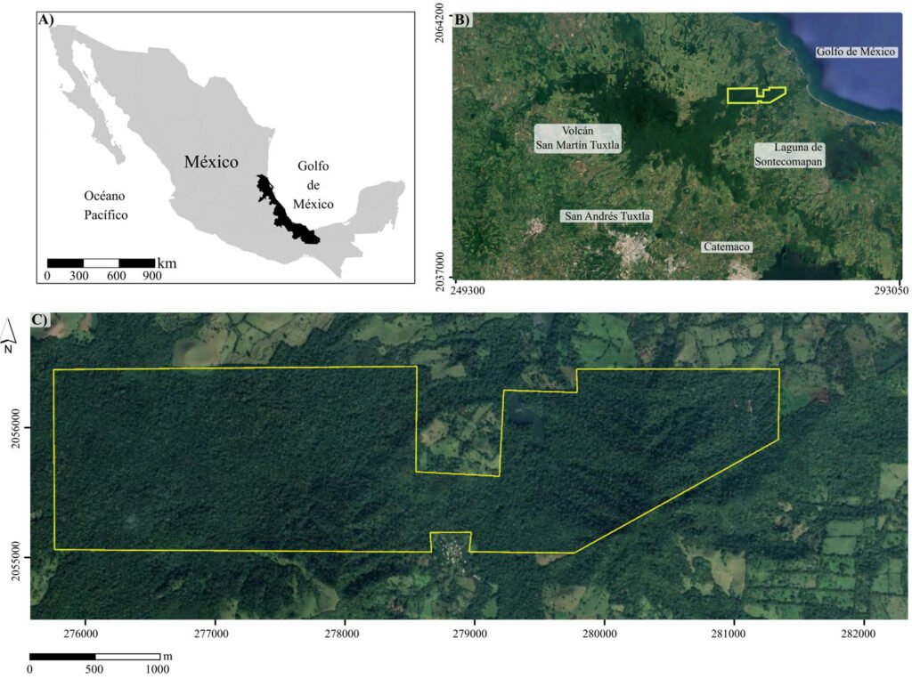
La vegetación cambia sus hojas de manera paulatina a lo largo del año, con algunas especies caducifolias (Ibarra-Manríquez, Martínez-Ramos et al., 1997), particular-
mente durante la época de secas, por ejemplo, Bernoullia flammea, Ceiba pentandra (ambas Malvaceae), Bursera simaruba (Burceraceae), Dussia mexicana, Erythrina folkersii, Vatairea lundelli (todas Fabaceae), Ficus isophlebia, Handroanthus guayacan (Bignoniaceae), Jacaratia dolichaula (Caricaceae) y Omphalea oleifera. La altura de los árboles del dosel puede alcanzar entre 10-20 m en las cimas de los cerros El Vigía o Cerro Azul (Lázaro Cárdenas), mientras que en sitios con menor pendiente pueden alcanzar de 30 a 40 m (Ibarra-Manríquez, Martínez-Ramos et al., 1997). Para información más detallada sobre la vegetación consultar Bongers et al. (1988), Popma et al. (1988), Manríquez, Ricker et al. (1997), Ibarra-Manríquez, Martínez-Ramos (1997), Navarrete-Segueda et al. (2021), Miranda-Gallegos et al. (2023) y Ek-Rodríguez et al. (2022, 2024, 2025).
La lista de especies para helechos y grupos afines está ordenada con base en PPG I (2016) y para las angiospermas la clasificación de APG IV (2016). Las familias, géneros y especies siguen un orden alfabético. La familia y especie con el que los integrantes de la flora fueron citados en Ibarra-Manríquez y Sinaca (1995, 1996a, b) fueron revisados y en caso de ser necesario, se actualizaron nomenclaturalmente con base en lo indicado por estudios taxonómicos (tabla 1), la revisión de las bases de datos POWO (2025) y Tropicos (2025), así como la consulta directa con taxónomos; estas fuentes de consulta fueron también usadas para indicar la distribución geográfica de cada especie.
La forma de crecimiento, hábito, altura de las especies, nombre común, así como la asociación con pastizales antropogénicos o vegetación ruderal de las especies, se derivaron de observaciones en campo realizadas de febrero de 1982 a junio de 2025, así como de la consulta de material depositado en el Herbario Nacional (MEXU) y el herbario de referencia que se encuentra en la ELT. Las formas de crecimiento y hábito siguen las definiciones de Moreno (1984). En particular, los árboles y arbustos fueron clasificados con base en su altura, ya que los primeros son plantas leñosas ≥ 3 m, mientras que los arbustos no superan este valor. En el caso de las especies con hábito trepador, las leñosas se denominan lianas, mientras que las que no presentan esta condición son trepadoras. Para las especies cuyo ejemplar tipo fue recolectado en la ELT, se indican los nombres de los colectores, el número de colecta y las siglas de los herbarios en los que se encuentran depositados el holotipo e isotipos. El listado excluye las especies cultivadas como Mangifera indica L. (Anacardiaceae) y Pachira aquatica Aubl. (Malvaceae).
Resultados
La lista compilada incluye 934 especies, 571 géneros y 139 familias (material suplementario). Entre los grupos de clasificación con jerarquía más alta (tabla 2; material suplementario), las Eudicotiledóneas son las que tienen una representación mayor respecto al número de familias (68.3%), géneros (67.4%) y especies (60.9%). Las 20 familias con mayor número de especies abarcan 59.1% de la flora, destacando Orchidaceae (108 especies), Asteraceae (61), Fabaceae (58), Rubiaceae (35) y Poaceae (28) (tabla 3). A nivel de género, los más relevantes al respecto son Epidendrum L. (16 especies), Piper L. (13), Ficus L. (10), así como Peperomia Ruiz et Pav. y Solanum L. (9 especies cada uno). Cuarenta y ocho familias (34.5%) y 410 géneros (71.8%) están representados por 1 especie. Un total de 27 especies fueron descritas como nuevas para la ciencia con base en colectas realizadas en la ELT; de 1997 a la fecha, 45 especies son integrantes adicionales de su flora (material suplementario).
Las formas de crecimiento más frecuentes fueron las hierbas (48.5%) y los árboles (27.7%); respecto al hábito de crecimiento, 77.6% de las especies son terrestres, seguidas en importancia por las trepadoras y epífitas que representan 17.3% y 16%, respectivamente (tabla 4). Las distribuciones geográficas con mayores registros de especies fueron las que se comparten exclusivamente entre México y Centroamérica (278 especies, 29.8%), ocupando el segundo sitio la agrupación formada por estas 2 áreas con Antillas y Sudamérica (217, 23.2%) (tabla 5). Catorce especies son cosmopolitas, 3 pantropicales y 14 introducidas (material suplementario). Un total de 93 especies (10%) son endémicas de México y 17 restringen su presencia a la región de Los Tuxtlas o Veracruz (tabla 6, fig. 6). Cerca de 24% de las especies se asocian con pastizales antropogénicos y vegetación ruderal (material suplementario), sin que se haya registrado su presencia en el bosque tropical perennifolio de la reserva, tanto en su fase madura como en etapas sucesionales tempranas o intermedias.
Discusión
Florística
La dominancia actual de las angiospermas entre las plantas vasculares del mundo es un hecho ampliamente documentado y se constata en el presente estudio (tabla 2), ya que engloban 91.5% de las especies, porcentaje prácticamente igual al que reportan Villaseñor et al. (2018) para toda la región de Los Tuxtlas (91.2%). El comparativo de la riqueza taxonómica reportado por Ibarra-Manríquez y Sinaca (1995, 1996a, b) y el del presente estudio no presentan diferencias cuantitativas notables a nivel de familias (139 y 138, respectivamente) ni de especies (940 y 934). Sin embargo, cualitativamente los cambios son numerosos (material suplementario). A nivel de familia, existen casos en que algunas de ellas han sido reconocidas como distintas (e.g., Phyllanthaceae, antes incluida en Euphorbiaceae; Dipentodontaceae, anteriormente en Celastraceae) o, por el contrario, como sinónimos (e.g., Asclepiadaceae de Apocynaceae; Bombacaceae y Tiliaceae de Malvaceae; Hippocrateaceae de Celastraceae; Myrsinaceae y Theophrastaceae de Primulaceae).
Tabla 1
Referencias florístico-taxonómicas consultadas para la elaboración del material suplementario. La etiqueta de varias incluye familias de helechos y licófitos.
| Familias | Referencias |
| Acanthaceae | Ramamoorthy y Uribe (1988), Daniel (2002, 2004, 2005) |
| Annonaceae | Ortiz-Rodriguez (2022), Ortiz-Rodríguez et al. (2024) |
| Apocynaceae | Morales (1997), Alvarado-Cárdenas et al. (2020) |
| Araceae | Krömer et al. (2019) |
| Arecaceae | Bacon y Bailey (2006), Henderson (2011) |
| Asteraceae | Villaseñor y Ortiz (2025) |
| Bromeliaceae | Espejo-Serna et al. (2005), Espejo-Serna y López-Ferrari (2018) |
| Celastraceae | Lombardi (2014), Biral (2021) |
| Costaceae | García-Mendoza e Ibarra-Manríquez (1991) |
| Cyperaceae | González-Elizondo et al. (2018) |
| Elaeocarpaceae | Palacios-Wassenaar y Castillo-Campos (2020) |
| Erythroxylaceae | Palacios-Wassenaar y Castillo-Campos (2019) |
| Fabaceae | Sousa y Rudd (1993), Pennington (1997), Zamora (2006), Sousa (2009, 2010), Aviles et al. (2022) |
| Gesneriaceae | Ramírez-Roa y Ibarra-Manríquez (1998), Clavijo et al. (2021), Ramírez-Roa et al. (2023) |
| Icacinaceae | Vera-Caletti y Wendt (2001) |
| Lamiaceae | Martínez-Gordillo et al. (2017) |
| Lauraceae | Rowher (1993), Lorea-Hernández (2002) |
| Loganiaceae | Islas-Hernández y Alvarado-Cárdenas (2023) |
| Malvaceae | Fryxell (1992) |
| Moraceae | Ibarra-Manríquez et al. (2012), Berg (2015), Hernández-Esquivel et al. (2020) |
| Orchidaceae | Salazar (1988) |
| Passifloraceae | Fragoso-Martínez y Castillo-Campos (2023) |
| Piperaceae | Vergara-Rodríguez et al. (2017), Callejas-Posada (2020), Carmona-Hernández et al. (2022) |
| Poaceae | Dávila et al. (2018) |
| Polygonaceae | Ancona et al. (2025) |
| Proteaceae | Edwards y Prance (2003) |
| Rubiaceae | Lorence y Nee (1987), Torres-Montúfar y Ochoterena (2013), Torres-Montúfar y Torres-Díaz (2022) |
| Sambucaceae | Villareal (2003) |
| Sapotaceae | Swenson et al. (2023) |
| Selaginellaceae | Zhou y Zhang (2023) |
| Smilacaceae | Ferrufino-Acosta (2010) |
| Thelypteridaceae | Riba (2009), Salino et al. (2015) |
| Urticaceae | Monro (2009) |
| Varias | Acebey et al. (2015), Smith y Tejero-Díez (2014), Krömer et al. (2020), Ruiz et al. (2025) |
Tabla 2
Síntesis taxonómica de la flora vascular de la Estación de Biología Tropical Los Tuxtlas.
| Taxones | Familias | Géneros | Especies |
| Lycopodiopsida | 2 | 4 | 11 |
| Polypodiopsida | 16 | 37 | 68 |
| Magnólidas | 9 | 21 | 55 |
| Monocotiledóneas | 17 | 124 | 231 |
| Eudicotiledóneas | 95 | 385 | 569 |
| Total | 139 | 571 | 934 |
Tabla 3
Familias y géneros con mayor número de especies en la zona de estudio.
| Familias | Especies | Géneros | Especies |
| Orchidaceae | 108 | Epidendrum | 16 |
| Asteraceae | 61 | Piper | 14 |
| Fabaceae | 58 | Ficus | 10 |
| Rubiaceae | 35 | Peperomia | 9 |
| Poaceae | 28 | Solanum | 9 |
| Euphorbiaceae | 26 | Eugenia | 8 |
| Araceae | 23 | Inga | 8 |
| Piperaceae | 23 | Passiflora | 8 |
| Solanaceae | 23 | Asplenium | 7 |
| Apocynaceae | 20 | Chamaedorea | 7 |
| Lauraceae | 19 | Cyperus | 7 |
| Bromeliaceae | 17 | Ocotea | 7 |
| Malvaceae | 17 | Begonia | 6 |
| Bignoniaceae | 16 | Desmodium | 6 |
| Moraceae | 16 | Lasiacis | 6 |
| Verbenaceae | 13 | Miconia | 6 |
| Arecaceae | 12 | Mikania | 6 |
| Melastomataceae | 12 | Philodendron | 6 |
| Polypodiaceae | 12 | Pleopeltis | 6 |
| Total | 539 (57.7%) | 152 (16.3%) |
Tabla 4
Número de especies de las formas de crecimiento y hábito de las plantas vasculares en la Estación de Biología Tropical Los Tuxtlas.
| Formas de crecimiento | Especies (%) | Hábito | Especies (%) |
| Árboles | 259 (27.7) | Epífitas | 149 (16) |
| Arbustos | 85 (9.1) | Hemiepífitas | 24 (2.6) |
| Helechos arborescentes | 3 (0.3) | Hemiparásitas | 3 (0.3) |
| Hierbas | 453 (48.5) | Rupícolas | 14 (1.5) |
| Palmas | 12 (1.3) | Parásitas | 1 (0.1) |
| Trepadoras leñosas (lianas) | 94 (10.1) | Terrestres | 725 (77.6) |
| Trepadoras herbáceas | 67 (7.2) | Trepadoras | 161 (17.3) |
Tabla 5
Número de especies de la flora vascular de la Estación de Biología Tropical Los Tuxtlas registradas en distintas áreas geográficas de América.
| País/región | Especies (%) |
| México | 93 (10) |
| México-Centroamérica | 278 (29.8) |
| México-Centroamérica-Antillas | 18 (1.9) |
| México-Centroamérica-Antillas-Sudamérica | 217 (23.2) |
| México-Centroamérica-Sudamérica | 198 (21.2) |
| México-Norteamérica | 1 (0.1) |
| México-Norteamérica-Centroamérica | 3 (0.3) |
| México-Norteamérica-Centroamérica | 2 (0.2) |
| México-Norteamérica-Centroamérica-Antillas-Sudamérica | 74 (7.9) |
| México-Sudamérica | 1 (0.1) |
En el material suplementario se puede revisar que 202 especies son actualmente consideradas como sinónimos y 48 han sido redeterminadas; en conjunto, representan 26.7% del total de la flora, con un promedio anual de 8.6 especies (1997-2025). En ambos casos, su clasificación actual puede incluso asociarse con distintos géneros, como lo ejemplifican Bolbitis bernoullii, sinónimo de Mickelia bernoullii (Dryopteridaceae), Oerstedianthus brevipes de Ardisia tuerckheimii (Primulaceae), Psychotria faxlucens de Palicourea faxlucens (Rubiaceae) o Rheedia edulis de Garcinia intermedia (Clusiaceae); en este rubro, destacan particularmente Bignoniaceae y Lauraceae, ya que alrededor de la mitad de sus especies fueron transferidas a otros géneros. Finalmente, se han descrito varias especies nuevas para la ciencia (material suplementario, tabla 6), que abarcan diversas formas de crecimiento y familias (e.g., Acanthaceae, Annonaceae, Gesneriaceae, Magnoliaceae, Polygonaceae, Proteaceae, Rubiaceae, Sapotaceae).
Las 15 familias con mayor número de especies concentran 52.5% del total registrado para la ELT (tabla 3) y al comparar este rubro con Villaseñor et al. (2018), nuevamente existe una coincidencia alta (50.8%). Ambos estudios concuerdan en 13 de ellas y de las 5 primeras, solo difieren en la posición particular que ocupan Orchidaceae, Asteraceae y Fabaceae. La jerarquía de estas familias se explica por su ubicación entre las más diversas de México y del continente americano (Ulloa et al., 2017; Villaseñor, 2016). Sin embargo, es conveniente considerar que 67.2 y 89.3% de las especies de Asteraceae y Poaceae, respectivamente, se registran únicamente en ambientes ruderales o pastizales de origen antropogénico (material suplementario). En el caso de los géneros con mayor diversidad, 9 de 15 concuerdan entre la región de Los Tuxtlas y el presente estudio, en particular Epidendrum (Orchidaceae), Piper y Peperomia (Piperaceae), Ficus (Moraceae), Solanum (Solanaceae) y Asplenium L. (Aspleniaceae). Los 3 primeros géneros son también encontrados entre los de mayor riqueza en México y América (Ulloa et al., 2017; Villaseñor, 2016).
En situación opuesta, 48 familias (34.5%) y 410 géneros (71.8%) tienen solo una especie en la ELT. Este resultado guarda relación con lo que se registra en México (Villaseñor, 2016), como acontece con Haemodoraceae y Lacistemataceae. Una situación análoga ocurre con numerosos géneros, entre los que pueden citarse Ampelocera Klotzsch (Ulmaceae), Aphananthe Planch. (Cannabaceae), Astrocaryum G. Mey (Arecaceae), Calophyllum L. (Calophyllaceae), Dialium L. (Fabaceae), Lunania Hook. (Salicaceae), Mosquitoxylum Krug et Urb. (Anacardiaceae), Nidema Britton et Millsp. (Orchidaceae), Ochroma Sw. (Malvaceae), Odontocarya Miers (Menispermaceae), Petrea L. (Verbenaceae), Pimenta Lindl. (Myrtaceae), Pleuranthodendron L.O. Williams (Salicaceae), Poulsenia Eggers (Moraceae), Sapindus L. (Sapindaceae), Tuxtla Villaseñor et Strother (Asteraceae) o Vatairea Aubl. (Fabaceae).
Tabla 6
Especies con distribución restringida a la región de Los Tuxtlas o al estado de Veracruz; se indica con un asterisco las que fueron descritas después de las publicaciones de Ibarra-Manríquez y Sinaca (1995, 1996a, b).
| Especies/área | Familia | Forma de crecimiento |
| Región de Los Tuxtlas | ||
| Capparidastrum tuxtlense* | Capparaceae | Árbol |
| Clethra tuxtlensis* | Clethraceae | Árbol |
| Costus dirzoi | Costaceae | Hierba |
| Drymonia mexicana* | Gesneriaceae | Arbusto |
| Hoffmannia altipetens* | Rubiaceae | Arbusto |
| Magnolia sinacacolinii* | Magnoliaceae | Árbol |
| Miconia ibarrae | Melastomataceae | Árbol |
| Mosannona depressa subsp. abscondita* | Annonaceae | Árbol |
| Piper marginecontinuum* | Piperaceae | Arbusto |
| Tridimeris tuxtlensis* | Annonaceae | Árbol |
| Veracruz | ||
| Arachnothryx pumae* | Rubiaceae | Árbol o arbusto |
| Croton sousae* | Euphorbiaceae | Árbol |
| Daphnopsis megacarpa | Thymelaeaceae | Arbusto |
| Eugenia colipensis | Myrtaceae | Árbol |
| Eugenia inirebensis | Myrtaceae | Árbol |
| Macroclinium pachybulbon | Orchidaceae | Hierba |
| Ruellia tuxtlensis | Acanthaceae | Hierba |
Formas de crecimiento y hábito
La fisonomía del bosque tropical perennifolio se debe a la abundancia y al tamaño de los árboles, primordialmente a los del estrato de mayor altura y la ELT no es la excepción al respecto (Bongers et al., 1988; Ibarra-Manríquez, Martínez-Ramos et al., 1997; Navarrete-Segueda et al., 2021). La importancia del componente arbóreo no se relaciona solo con la estructura de los bosques (e.g., contribución a la biomasa), sino también por su desempeño en aspectos funcionales, como la captura de carbono y las interacciones que mantiene con polinizadores y frugívoros (Beckman y Sullivan, 2023; Fuster, et al., 2018; Lutz et al., 2018; Ollerton, 2017; Spicer et al., 2020). Si bien en la ELT esta forma de crecimiento es relevante por su número de especies (259; 27.7%), es superada ampliamente por las hierbas (453, 48.5%).
Este patrón de dominancia del número de especies de hierbas respecto a los árboles debe destacarse en los estudios florísticos de los bosques tropicales, puesto que ha sido registrado previamente (Ibarra-Manríquez et al., 2021; Linares-Palomino et al., 2009; Meave et al., 2017; Rojas-Martínez y Flores-Olvera, 2019). A nivel de bioma, este patrón de riqueza se mantiene, ya que la proporción de hierbas y árboles es de 45% y 30%, respectivamente (Spicer et al., 2020). Para la flora de México, Villaseñor y Ortiz (2014) destacaron la predominancia de las hierbas perennes o anuales (13,408) sobre los árboles (4,044), un aspecto que había sido sugerido primeramente por Rzedowski (1991a). Como una consecuencia de lo anterior, el hábito terrestre es el preponderante en la ELT (77.6%), debido al efecto aditivo de la riqueza de las hierbas y árboles, aunado al aporte de las trepadoras, tanto leñosas como herbáceas. Para los bosques tropicales, Spicer et al. (2020) concuerdan en resaltar la dominancia de este hábito, al englobar 80% de las especies, con el remanente adscrito a las epífitas.
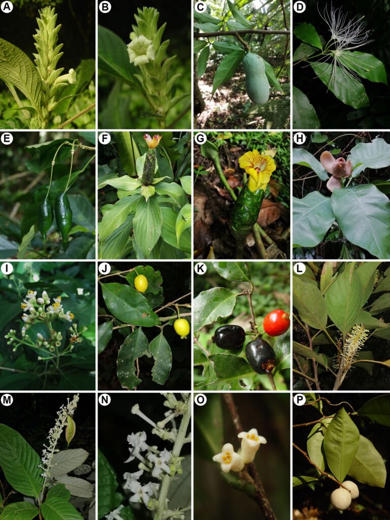
Distribución geográfica y endemismo
El 29.8% de la flora vascular de la ELT se comparte exclusivamente con Centroamérica, mientras que 21.2% se registra en esta área en conjunto con Sudamérica (tabla 5), posiciones que coinciden con lo reportado por Villaseñor et al. (2003) en su estudio biogeográfico de los bosques tropicales húmedos de México (31.4 y 12.7%, respectivamente). Estas afinidades biogeográficas también coinciden con Wendt (1993), quien determinó que el componente arbóreo del dosel de los bosques tropicales de México tenía sus mayores nexos con Centroamérica y con lo destacado por Rzedowski (1991a, b), en relación con las afinidades marcadamente meridionales del bosque tropical perennifolio de México.
Al respecto, es interesante destacar las distribuciones vicariantes de 4 especies, que sólo se han recolectado en la región de Los Tuxtlas y en localidades de Costa Rica (Haydenoxylon calzadae [Celastraceae], Styphnolobium parviflorum [Fabaceae] y Tuxtla pittieri [Asteraceae]) y Honduras (Justicia tuxtlensis [Acanthaceae]), lo que demanda estudios más detallados para explicarlas debidamente, ya que no parecen asociarse a una exploración deficiente de la flora, tomando en cuenta los distintos proyectos florísticos que se están implementando desde hace décadas en la región mesoamericana (e.g., Flora de Costa Rica, Flora de Nicaragua, Flora Mesoamericana).
Por otro lado, se debe discutir lo expuesto por Villaseñor et al. (2018), quienes resaltaron que 6 especies de la región de Los Tuxtlas solo se encuentran en la ELT, lo cual no es correcto para Justicia tuxtlensis, debido a su distribución vicariante previamente expuesta. Esta aseveración tampoco es válida para Capparidastrum tuxtlense (Capparaceae) y Hoffmannia altipetens (Rubiaceae), ya que han sido colectadas tanto en la ELT como en otras localidades de la región. Las 3 especies restantes carecen de registros que certifiquen su presencia en la reserva. Styrax tuxtlensis P.W. Fritsch (Styracaceae) se conoce únicamente de un registro proveniente del volcán Santa Marta, lo que hace muy improbable su presencia en la ELT. En el caso de Guadua tuxtlensis Londoño et Ruiz-Sánchez (Poaceae), es factible que pueda ser colectada en los perímetros de la ELT que colindan con pastizales para la crianza de ganado (fig. 1), ya que es uno de los tipos de vegetación en los que se le ha reportado. De igual manera, la presencia de Diospyros tuxtlensis Provance et A.C. Sanders (Ebenaceae) es viable considerando su colecta en localidades no tan lejanas al oeste de la reserva. Hasta ahora, las especies que se conocen exclusivamente de la ELT son Piper marginecontinuum (Piperaceae) y Tridimeris tuxtlensis (Callejas Posada, 2020; Ortiz-Rodríguez et al., 2024).
La flora endémica de México registrada en la ELT representa 10% del total, una cifra mayor que la sugerida por Rzedowski (1991a) para el bosque tropical perennifolio (5%), similar (9.6%) a la que reportó Wendt (1993) y menor (20.5%) que la citada en Villaseñor et al. (2003). A pesar de la discrepancia de estos valores, existe concordancia en que la región de Los Tuxtlas ha desempeñado un papel relevante como área de concentración de especies arbóreas endémicas (Wendt, 1993), junto con el norte de Oaxaca (Tuxtepec) y el SE de Veracruz (Uxpanapa). Las marcadas similitudes florísticas del bosque tropical húmedo de Veracruz son mayores con Chiapas, Oaxaca, Tabasco y Puebla (Villaseñor y Ortiz, 2025). A nivel de familia, es interesante señalar que 7 de las 8 especies registradas de Gesneriaceae son endémicas de México.
Como conclusiones generales del estudio se debe resaltar que la actualización taxonómica de la flora vascular de la ELT modifica el reconocimiento de una proporción importante de especies, géneros y familias, y por su relevancia, es una actividad que requiere de actualizaciones continuas. Lo dinámico de este proceso se refleja en la tasa de cambios nomenclaturales registrada para la reserva de 1997 a la fecha (8.6 especies anualmente). Se espera que la presente contribución facilite recabar información de diferentes áreas del conocimiento sobre las especies citadas en el material suplementario, por ejemplo, coordinar iniciativas para la restauración regional (Ibarra-Manríquez, 2017). El número de especies registrado en esta área protegida (934 especies) representa 27.8% de las 3,362 que citan Villaseñor y Ortiz (2025) para este bioma en Veracruz, un porcentaje muy importante si se considera la pequeña extensión de esta reserva (640 ha).
Se recomienda continuar con el inventario de la ELT, con el objetivo de cuantificar la composición florística actual con más detalle, que permita, entre otras cosas, detectar la abundancia de las especies y realizar actividades que promuevan su conservación, particularmente para aquellas poco abundantes o con una distribución restringida a ciertas áreas de la ELT (Ibarra-Manríquez, Martínez-Ramos et al., 1997); lo anterior podría ser más aplicable para las especies que registran un bajo número de exsiccatas (material suplementario). Sin duda alguna, esta actividad prioritaria también podría identificar especies nuevas para la ciencia, como lo demuestran los hallazgos registrados desde la década de los 80 hasta la fecha. Una evidencia que respalda lo anterior es que el material tipo de 27 especies fue recolectado dentro de los límites territoriales de la ELT (material suplementario), de las cuales 15 fueron descritas de 1997 a la fecha. Se espera que el presente estudio fomente acciones para conservar el valioso patrimonio biológico del bosque tropical húmedo que resguarda la ELT, límite más norteño de este tipo de vegetación en América. Se debe valorar aún más este papel, especialmente si se considera su localización en elevaciones bajas, que, debido a diversos factores, cada vez tiene menor extensión en la región de Los Tuxtlas (Bonilla-Moheno y Aide, 2020; von Thaden et al., 2020). También sería extremadamente valioso atemperar el deterioro biológico señalado por Ibarra-Manríquez (2017), especialmente en las partes con mayor acceso a actividades humanas.
Agradecimientos
Dos árbitros anónimos y M. Socorro González-Elizondo, en su calidad de editora asociada, aportaron valiosas sugerencias para mejorar una primera versión del presente estudio. Agradecemos a los taxónomos que amablemente revisaron las especies de las familias de su especialidad: Leonardo O. Alvarado-Cárdenas (Apocynaceae), Thomas F. Daniel (Acanthaceae), Mario Adolfo Espejo Serna (Bromeliaceae), Francisco Gerardo Lorea Hernández (Lauraceae). Se reconoce el apoyo de Armando Navarrete Segueda en la elaboración de la figura 1 y finalmente, el de María Antonieta Arizmendi Espinosa en las distintas fases editoriales para finalizar esta publicación.
Referencias
Acebey, A. R., Krömer, T., Vázquez-Torres, M. y Tejero-Díez, J. D. (2015). Helechos y licofitos de la Reserva de la Biosfera Los Tuxtlas, Veracruz, México. Botanical Sciences, 93, 1–32. https://doi.org/10.17129/botsci.124
Alvarado-Cárdenas, L. O., Lozada-Pérez, L., Islas-Hernández, C. S., Cortez, E. B., Maya-Mandujano, K. G. y Chávez-Hernández, M. G. (2020). Apocináceas de ayer y hoy. Conocimiento histórico y reevaluación de la diversidad y distribución de Apocynaceae en México. Botanical Sciences, 98, 393–416. https://doi.org/10.17129/botsci.2525
Ancona, J. J., Ortiz-Díaz, J. J. y Hernández-Ledesma, P. (2025). Eight new species of Coccoloba sect. Campderia (Polygonaceae, Eriogonoideae) from Mexico and Central America. Acta Botanica Mexicana, 132, e2435. https://doi.org/10.21829/abm132.2025.2435
Antonelli, A., Fry, C., Smith, R. J., Eden, J., Govaerts, R. H. A., Kersey, P. et al. (2023). State of the World’s plants and fungi 2023. Royal Botanic Gardens, Kew. England. https://doi.org/10.34885/wnwn-6s63
APG IV (The Angiosperm Phylogeny Group). (2016). An update of the Angiosperm Phylogeny Group classification for the orders and families of flowering plants: APG IV. Botanical Journal of the Linnean Society, 181, 1–20. https://doi.org/10.1111/boj.12385
Aviles, P. G., Koenen, E. J. M., Riina, R., Hughes, C. E., Ringelberg, J. J., Carnevali Fernández-Concha, G. et al. (2022). Re-establishment of the genus Pseudalbizzia (Leguminosae, Caesalpinioideae, mimosoid clade): the New World species formerly placed in Albizia. Phytokeys, 205, 371–400. https://doi.org/10.3897/phytokeys.205.76821
Bacon, C. D. y Bailey, C. D. (2006). Taxonomy and conservation: a case study from Chamaedorea alternans. Annals of Botany, 98, 755–763. https://doi.org/10.1093/aob/mcl158
Beckman, N. G. y Sullivan, L. L. (2023). The causes and consequences of seed dispersal. Annual Review of Ecology, Evolution, and Systematics, 54, 403–427. https://doi.org/10.1146/annurev-ecolsys-102320-104739
Berg, C. C. (2015). Moraceae. En G. Davidse, M. Sousa, S. Knapp y F. Chiang (Eds.), Flora Mesoamericana, Saururaceae a Zygoplyllaceae (pp. 90–116). St. Louis Missouri: Sheridan Books.
Biral, L. (2021). A new combination and a new synonym in Haydenoxylon (Celastraceae). Novon, 29, 74–76. https://doi.org/10.3417/2021646
Bongers, F., Popma, J., Meave-del Castillo, J. y Carabias, J. (1988). Structure and floristic composition of the lowland rain forest of Los Tuxtlas, Mexico. Vegetatio, 74, 55–80. https://doi.org/10.1007/BF00045614
Bonilla-Moheno, M. y Aide, T. M. (2020). Beyond deforestation: land cover transitions in Mexico. Agricultural Systems,
178, 102734. https://doi.org/10.1016/j.agsy.2019.102734
Callejas-Posada, R. (2020). Piperaceae. En G. Davidse, C. Ulloa-Ulloa, H. Hernández-Macías y S. Knapp (Eds.) Flora Mesoamericana (pp. 1–590). St. Louis Missouri: Sheridan Books.
Campos, V. A., Kelly, L. M. y Delgado, S. A. (2004). Bejucos y otras trepadoras de la Estación de Biología Tropical Los Tuxtlas, Veracruz, México. México D.F.: Instituto de Biología, Universidad Nacional Autónoma de México.
Carmona-Hernández, O., Laccetti, L., Martínez-Hernández, M. D. J., Luna-Rodríguez, M., Fernández, M. D. S., Guerrero-Analco, J. A. et al. (2023). Plant conservation in the Mesoamerican biodiversity hotspot: a case study on the Piper genus in Veracruz (Mexico). Tropical Ecology, 64, 324–336. https://doi.org/10.1007/s42965-022-00271-9
Clavijo, L., Ramírez-Roa A. y Clark, J. L. (2021). Drymonia mexicana (Gesneriaceae), a new endemic species from Veracruz (Mexico). Journal of the Botanical Research Institute of Texas, 15, 60–63. https://doi.org/10.17348/jbrit.v15.i1.1050
Conanp (Comisión Nacional de Áreas Naturales Protegidas). (2006). Programa de conservación y manejo Reserva de la Biosfera Los Tuxtlas. México D.F.: Comisión Nacional de Áreas Naturales Protegidas.
Cornejo-Tenorio, G., Ibarra-Manríquez, G. y Sinaca-Colín, S. (2019). Flora de Los Tuxtlas. Guía Ilustrada. México D.F.: Universidad Nacional Autónoma de México.
Daly, M., Herendeen, P. S., Guralnick, R. P., Westneat, M. W. y McDade, L. (2012). Systematics agenda 2020: the mission evolves. Systematic Biology, 61, 549–552. https://doi.org/10.1093/sysbio/sys044
Daniel, T. F. (2002). New and reconsidered Mexican Acantha-
ceae IX. Justicia. Proceedings of the California Academy of Sciences, 53, 37–49.
Daniel, T. F. (2004). Further range extensions of Mexican Acanthaceae. Polibotánica, 18, 1–12.
Daniel, T. F. (2005). Catalog of Honduran Acanthaceae with taxonomic and phytogeographic notes. Contributions from the University of Michigan Herbarium, 24, 51–108.
Dávila, P., Mejía-Saulés, M. T., Soriano-Martínez, A. M. y Herrera-Arrieta, Y. (2018). Conocimiento taxonómico de la familia Poaceae en México. Botanical Sciences, 96, 462–514. https://doi.org/10.17129/botsci.1894
Edwards, K. S. y Prance, G. Y. (2003). Four new species of Roupala (Proteaceae). Brittonia, 55, 61–68. https://www.jstor.org/stable/3218415?seq=1
Ek-Rodríguez, I. L., Coates, R., Sinaca-Colín, S. e Ibarra-Manríquez, G. (2022). Liana community attributes in one of the northernmost neotropical rainforests. Botanical Sciences, 100, 353–369. https://doi.org/10.17129/botsci.2955
Ek-Rodríguez, I. L., Meave, J. A., Navarrete-Segueda, A., González-Arqueros, M. L. e Ibarra- Manríquez, G. (2024). Environmental heterogeneity influences liana community differentiation across a neotropical rainforest landscape. Ecology et Evolution, 14, e11170. https://doi.org/10.1002/ece3.11170
Ek-Rodríguez, I. L., Navarrete-Segueda, A., Siebe, C., Meave, J. A., Vela-Correa, G. e Ibarra- Manríquez, G. (2025). Relief, soil and tree community attributes jointly shape liana community structure and diversity in a Neotropical rainforest landscape. Catena, 255, 109017. https://doi.org/10.1016/j.catena.2025.109017
Espejo-Serna, A. y López-Ferrari, A. R. (2018). La familia Bromeliaceae en México. Botanical Sciences, 96, 533–554. https://doi.org/10.17129/botsci.1918
Espejo-Serna, A., López-Ferrari, A. R. y Ramírez-Morillo, I. (2005). Bromeliaceae. Flora de Veracruz. Xalapa: Instituto de Ecología, A.C. Flora de Veracruz. https://doi.org/10.21829/fv.343.2005.136
Fragoso-Martínez, I. y Castillo-Campos, G. (2023). Passifloraceae. Flora de Veracruz. Xalapa: Instituto de Ecología, A.C. Flora de Veracruz. https://doi.org/10.21829/fv.585.20
23.200
Ferrufino-Acosta, L. (2010). Taxonomic revision of the genus Smilax (Smilacaceae) in Central America and the Caribbean Islands. Willdenowia, 40, 227–280. https://doi.org/10.3372/wi.40.40208
Fuster, F., Kaiser-Bunbury, C., Olesen, J. M. y Traveset, A. (2018). Global patterns of the double mutualism pheno-
menon. Ecography, 42, 826–835. https://doi.org/10.1111/ecog.04008
Fryxell, P. A. (1992). Malvaceae. Flora de Veracruz. Xalapa: Instituto de Ecología, A.C. Flora de Veracruz. https://doi.org/10.21829/fv.420.1992.68
García-Mendoza, A. e Ibarra-Manríquez, G. (1991). A new species of Costus (Costoideae, Zingiberaceae) from Veracruz, Mexico. Annals of the Missouri Botanical Garden, 78, 1081–1084. https://doi.org/10.2307/2399745
González-Elizondo, M. S., Reznicek, A. A. y Tena-Flores, J. A. (2018). Cyperaceae in Mexico: diversity and distribution. Botanical Sciences, 96, 305–331. https://doi.org/10.17129/botsci.1870
Gutiérrez-García, G. y Martin, R. (2011). Climate and climate change in the region of Los Tuxtlas (Veracruz, Mexico): a statistical analysis. Atmósfera, 24, 347–373.
Henderson, A. (2011). A revision of Geonoma (Arecaceae). Phytotaxa, 17, 1–271. https://doi.org/10.11646/phytotaxa.
17.1.1
Hernández-Esquivel, K., Piedra-Malagón, E. M., Cornejo-Tenorio, G., Mendoza-Cuenca, L., González-Rodríguez, A., Ruiz-Sánchez, E. et al. (2020). Unraveling the extreme morphological variation in the neotropical Ficus aurea complex (subg. Spherosuke, sect. Americanae, Moraceae). Journal of Systematics and Evolution, 58, 263–281. https://doi.org/10.1111/jse.12564
Ibarra-Manríquez, G. (1988). The palms of a tropical rain forest in Veracruz, Mexico. Principes, 32, 147–155.
Ibarra-Manríquez, G. (2017). Avances en la investigación botánica en la Estación de Biología Tropical Los Tuxtlas ¿Qué hacer ahora? En V. H. Reynoso, R. I. Coates y C. M. L. Vázquez (Eds.), Avances y perspectivas en la investigación de los bosques tropicales y sus alrededores: la región de Los Tuxtlas (pp. 101–116). Ciudad de México: Instituto de Biología, Universidad Nacional Autónoma de México.
Ibarra-Manríquez, G., Cornejo-Tenorio, G., González-Castañeda, N., Piedra-Malagón, E. M. y Luna, A. (2012). El género Ficus L. (Moraceae) en México. Botanical
Sciences, 90, 389–452. https://doi.org/10.17129/botsci.472
Ibarra-Manríquez, G., Cornejo-Tenorio, G., Hernández-Esquivel, K. B., Rojas-López, M., Sánchez-Sánchez, L. (2021). Vegetación y flora vascular del ejido Llano de Ojo de Agua, Depresión del Balsas, municipio de Churumuco, Michoacán, México. Revista Mexicana de Biodiversidad, 92, e923482. https://doi.org/10.22201/ib.20078706e.2021.92.3482
Ibarra-Manríquez, G., Martínez-Morales, M. y Cornejo-Tenorio, G. (2015). Frutos y semillas del bosque tropical perennifolio. región de Los Tuxtlas. Veracruz. Ciudad de México: Comisión Nacional para el Conocimiento y Uso de la Biodiversidad.
Ibarra-Manríquez, G., Martínez-Ramos, M., Dirzo, M. y Núñez-Farfán, J. (1997). La Vegetación. En S. E. Gónzález, R. Dirzo y R. C. Vogt (Eds.), Historia natural de Los Tuxtlas (pp. 61–85). Ciudad de México: Universidad Nacional Autónoma de México.
Ibarra-Manríquez, G., Ricker, M., Ángeles, G., Sinaca-Colín, S. y Sinaca-Colín, M. A. (1997). Useful plants of the Los Tuxtlas rain forest (Veracruz, Mexico): considerations of their market potential. Economic Botany, 51, 362–376. https://doi.org/10.1007/BF02861046
Ibarra-Manríquez, G. y Sinaca-Colín, S. (1987). Lista florística de la Estación de Biología Tropical Los Tuxtlas. Listados Florísticos de México VII. México D.F.: Instituto de Biología, Universidad Nacional Autónoma de México.
Ibarra-Manríquez, G. y Sinaca-Colín, S. (1995). Lista florís-
tica comentada de la Estación de Biología Tropical “Los Tuxtlas”, Veracruz, México. Revista de Biología Tropical, 43, 75–115.
Ibarra-Manríquez, G. y Sinaca-Colín, S. (1996a). Lista florística comentada de la Estación de Biología Tropical Los Tuxtlas, Veracruz. México: Mimosaceae a Verbenaceae. Revista de Biología Tropical, 44, 41–60.
Ibarra-Manríquez, G. y Sinaca-Colín, S. (1996b). Lista comentada de plantas de la Estación de Biología Tropical Los Tuxtlas, Veracruz, México (Violaceae-Zingiberaceae). Revista de Biología Tropical, 44, 427–447.
Islas-Hernández, C. S. y Alvarado-Cárdenas, L. O. (2023). Sinopsis del género Spigelia (Loganiaceae) en Norteamérica, Centroamérica y el Caribe. Acta Botanica Mexicana, 130, e2202. https://doi.org/10.21829/abm130.2023.2202
Krömer, T., Acebey, A. R., Armenta-Montero, S. y Croat, T. B. (2019). Diversity, distribution, and conservation status of Araceae in the state of Veracruz, Mexico. Annals of the Missouri Botanical Garden, 104, 10–32. https://doi.org/10.3417/2018214
Krömer, T., Espejo-Serna, A., López-Ferrari A. R., Acebey, A. R., García-Cruz, J. y Mathieu, G. (2020). Las angiospermas epífitas del estado de Veracruz, México: diversidad y distribución. Revista Mexicana de Biodiversidad, 91, e913
415. https://doi.org/10.22201/ib.20078706e.2020.91.3415
Linares-Palomino, R., Cardona, V., Hennig, E. I., Hensen, I., Hoffmann, D., Lendzion, J. et al. (2009). Non-woody life-form contribution to vascular plant species richness in a tropical American forest. Plant Ecology, 201, 87–99. https://doi.org/10.1007/s11258-008-9505-z
Liu, Y., Borregaard, M. K., Xu, X., Dimitrov, D., Pellissier, L., Shrestha, N. et al. (2023). An updated floristic map of the world. Nature Communications, 14, 2990. https://doi.org/10.1038/s41467-023-38375-y
Lombardi, J. A. (2014). Celastraceae (Hippocrateoideae e Salacioideae). Flora Neotropica, 114, 1–227.
Lorea-Hernández, F. G. (2002). La familia Lauraceae en el sur de México: diversidad, distribución y estado de conservación. Botanical Sciences, 71, 59–70. https://doi.org/10.17129/botsci.1663
Lorence, D. H. y Nee, M. (1987). Randia retroflexa (Rubiaceae), a new species from southern Mexico. Brittonia, 39, 371–375. https://doi.org/10.2307/2807136
Lutz, J. A., Furniss, T. J., Johnson, D. J., Davies, S. J., Allen, D., Alonso, A. et al. (2018). Global importance of large-diameter trees. Global Ecology and Biogeography, 27, 849–864. https://doi.org/10.1111/geb.12747
Martin-Del Pozzo, A. L. (1997). Geología. En E. Gónzález, R. Dirzo y R. C. Vogt (Eds.). Historia natural de Los Tuxtlas (pp. 25–31). Ciudad de México: Universidad Nacional Autónoma de México.
Martínez-Gordillo, M., Bedolla-García, B., Cornejo-Tenorio, G., Fragoso-Martínez, I., García-Peña, M. R., González-Gallegos, J. G. et al. (2017). Lamiaceae de México. Botanical Sciences, 95, 780–806. https://doi.org/10.17129/botsci.1871
Meave, J. A., Rincón-Gutiérrez, A., Ibarra-Manríquez, G., Gallardo-Hernández, C., Romero-Romero, M. A. (2017). Checklist of the vascular flora of a portion of the hyper-humid region of La Chinantla, Northern Oaxaca Range, Mexico. Botanical Sciences, 95, 722–759. https://doi.org/10.17129/botsci.1812
Miranda, F. y Hernández, E. (1963). Los tipos de vegetación de México y su descripción. Botanical Sciences, 28, 29–179. https://doi.org/10.17129/botsci.1084
Miranda-Gallegos, K. V., Navarrete-Segueda, A., Cortés-Flores, J., González-Arqueros, M. L., Acosta-Pérez, E. E. e Ibarra-Manríquez, G. (2023). Landscape heterogeneity drives spatial distribution of palm community in a Neotropical rainforest reserve affected by defaunation. Botanical Sciences, 101, 654–669. https://doi.org/10.17129/botsci.3204
Monro, A. K. (2009). Two new species and a nomenclatural synopsis of Myriocarpa (Urticaceae) from Mesoamerica. Novon, 19, 85–95. https://doi.org/10.3417/2006211
Morales, J. F. (1997). A synopsis of the genus Prestonia (Apocynaceae) section Tomentosae in Mesoamérica. Novon, 7, 59–66. https://doi.org/10.2307/3392074
Moreno, N. P. (1984). Glosario botánico ilustrado. México D.F.: Compañía Editorial Continental, S.A. de C.V.
Navarrete-Segueda, A., Cortés-Flores, J., Cornejo-Tenorio, G., González-Arqueros, L., Torres-García, M. e Ibarra-Manríquez, G. (2021). Timber and non-timber forest products in the northernmost Neotropical rainforest: ecological factors unravel their landscape distribution. Journal of Environmental Management, 279, 111819. https://doi.org/10.1016/j.jenvman.2020.111819
Ollerton, J. (2017). Pollinator diversity: distribution, ecological function, and conservation. Annual Review of Ecology, Evolution and Systematics, 48, 353–376. https://doi.org/10.1146/annurev-ecolsys-110316-022919
Ortiz-Rodríguez, A. E. (2022). Naming the long-known: a new species of Desmopsis (Annonaceae) endemic to Mexico. Acta Botanica Mexicana, 129, e2110. https://doi.org/10.21829/abm129.2022.2110
Ortiz-Rodríguez, A. E., Nge, F. J., Rodrígues‑Vaz, C., Soulé, V., Schatz, G. E., Martínez‑Velarde, M. F. et al. (2024). Taxonomy, systematics and conservation of the highly threatened and endemic Mexican genus Tridimeris (Annonaceae). Plant Systematics and Evolution, 310, 47. https://doi.org/10.1007/s00606-024-01929-8
Palacios-Wassenaar O. M. y Castillo-Campos, G. (2019). Erythroxylaceae. Flora de Veracruz. Xalapa. Instituto de Ecología, A.C. https://doi.org/10.21829/fv.43.2019.182
Palacios-Wassenaar O. M. y Castillo-Campos, G. (2020). Elaeocarpaceae. Flora de Veracruz. Xalapa. Instituto de Ecología, A.C. https://doi.org/10.21829/fv.489.2020.185
Pennington, T. D. (1997). The genus Inga: botany. Belgium: The Royal Botanic Gardens, Kew. Continental Printing.
Popma, J., Bongers, F. y Meave-del Castillo, J. (1988). Patterns in the vertical structure of the tropical lowland rain forest of Los Tuxtlas, Mexico. Vegetatio, 74, 81–91. https://doi.org/10.1007/BF00045615
POWO (2025). Plants of the World Online. Facilitated by the Royal Botanic Gardens, Kew. Recuperado 13 abril, 2025, de: https://powo.science.kew.org/
PPG (The Pteridophyte Phylogeny Group) 1. (2016). A community-derived classification for extant lycophytes and ferns. Journal of Systematics and Evolution, 54,
563–603. https://doi.org/10.1111/jse.12229
Ramamoorthy, T. P. y Uribe, Y. H. (1988). A new name and a new species in Mexican Ruellia (Acanthaceae). Plant Systematic and Evolution, 159, 161–163. https://doi.org/10.1007/BF00935968
Ramírez-Roa, A. e Ibarra-Manríquez, G. (1998). A new species of Solenophora (Gesneriaceae) from southeast Veracruz, Mexico. Novon, 7, 281–284. https://doi.org/10.2307/3391945
Ramírez-Roa, A., Paniagua-Ibáñez, M. y Mora-Jarvio, M. A. (2023). Gesneriaceae. Flora de Veracruz. Xalapa: Instituto de Ecología, A.C. https://doi.org/10.21829/fv.579.2023.199
Raven, P. H., Gereau, R. E., Phillipson, P. B., Chatelain, C., Jenkins, C. N. y Ulloa, U. C. (2020). The distribution of biodiversity richness in the tropics. Science Advances, 6, eabc6228. https://doi.org/10.1126/sciadv.abc6228
Reynoso, V. H., Coates, R. I. y Vázquez, C. M. L. (Eds.). (2017). Avances y perspectivas en la investigación de los bosques tropicales y sus alrededores: la región de Los Tuxtlas. Ciudad de México: Instituto de Biología, Universidad Nacional Autónoma de México.
Riba, R. (1989). A new species of Thelypteris subg. Goniopteris from the state of Veracruz, Mexico. American Fern Journal, 79, 122–124. https://doi.org/10.2307/1547294
Rojas-Martínez, C. y Flores-Olvera, H. (2019). Florística de la sierra El Pelado, Acatlán, Puebla, México. Revista Mexicana de Biodiversidad, 90, e902694. https://doi.org/10.22201/ib.20078706e.2019.90.2694
Rowher, J. G. (1993). Lauraceae: Nectandra. Flora Neotropica, 60, 1https://doi.org/10.17129/botsci.3673332.
Ruiz, G. M. G., Gómez D. J. A. y Krömer, T. (2025). Las plantas vasculares endémicas de Veracruz: análisis de 30 años de conocimiento. Botanical Sciences, 103, 876–898. https://doi.org/10.17129/botsci.3673
Rzedowski, J. (1978). Vegetación de México. México D.F.: Limusa.
Rzedowski, J. (1991a). El endemismo en la flora fanerogámica mexicana: una apreciación analítica preliminar. Acta Botanica Mexicana,15, 47–64. https://doi.org/10.21829/abm15.1991.620
Rzedowski, J. (1991b). Diversidad y orígenes de la flora fanerogámica de México. Acta Botanica Mexicana, 14, 3–21. https://doi.org/10.21829/abm14.1991.611
Salazar, G. A. (1988). Mormodes tuxtlensis, nueva especie de Veracruz, México. Orquídea (Méx.), 11, 51–62.
Salino, A., Almeida, T. E. y Smith, A. R. (2015). New combinations in Neotropical Thelypteridaceae. Phytokeys, 57, 11–50. https://doi.org/10.3897/phytokeys.57.5641
Sánchez-Garfias, B., Ibarra-Manríquez, G. y González-García, L. (1991). Manual de identificación de frutos y semillas anemócoros de árboles y lianas de la Estación “Los Tuxtlas”, Veracruz, México. Cuadernos 12. México D.F.: Instituto de Biología, Universidad Nacional Autónoma de México.
Sarukhán, J., Urquiza-Haas, T., Koleff, P., Carabias, J., Dirzo, R., Ezcurra, E. et al. (2015). Strategic actions to value, conserve, and restore the natural capital of megadiversity countries: the case of Mexico. BioScience, 65, 164–173. https://doi.org/10.1093/biosci/biu195
Smith, A. R. y Tejero-Díez, J. D. (2014). Pleopeltis (Polypodiaceae), a redefinition of the genus and nomenclatural novelties. Botanical Sciences, 92, 43–58. https://doi.org/10.17129/botsci.29
Soto, M. y Gama, L. (1997). Climas. En E. González, R. Dirzo y R. C. Vogt (Eds.), Historia natural de Los Tuxtlas (pp. 7–23). México D.F.: Universidad Nacional Autónoma de México.
Sousa, S. M. (2009). Adiciones al género Inga (Ingeae, Mimosoideae, Leguminosae) para la Flora Mesoamericana. Acta Botanica Mexicana, 89,25–41. https://doi.org/10.21829/abm89.2009.303
Sousa, S. M. (2010). Revisión del complejo de Lonchocarpus cruentus (Leguminosae: Papilionoideae: Millettieae), con descripciónes de cinco especies nuevas. Brittonia, 62, 321–336. https://doi.org/10.1007/s12228-009-9116-6
Sousa, S. M. y Rudd, V. E. (1993). Revision del género Styphnolobium (Leguminosae: Papilionoideae: Sophoreae). Annals of the Missouri Botanical Garden, 80, 270–283. https://doi.org/10.2307/2399827
Spicer, M. E., Mellor, H. y Carson, A. P. (2020). Seeing beyond the trees: a comparison of tropical and temperate plant growth forms and their vertical distribution. Ecology, 101, e02974. https://doi.org/10.1002/ecy.2974
Swenson, U., Lepschi, B., Lowry, P. P. II, Terra-Araujo, M. H., Santos, K., Nylinder, S. et al. (2023). Reassessment of generic boundaries in Neotropical Chrysophylloideae (Sapotaceae): eleven reinstated genera and narrowed circumscriptions of Chrysophyllum and Pouteria. Taxon, 72, 307–359. https://doi.org/10.1002/tax.12894
Torres-Montúfar, A. y Ochoterena, H. (2013). Dos especies nuevas de la familia Rubiaceae de la sierra de los Tuxtlas, Veracruz, México. Revista Mexicana de Biodiversidad, 84, 1082–1089. https://doi.org/10.7550/rmb.32503
Torres-Montúfar, A. y Torres-Díaz, A. N. (2022). Las Rubiáceas de México: ¿Ya está hecho el trabajo? Botanical Sciences, 100, 446–468. https://doi.org/10.17129/botsci.2847
Tropicos. (2025). Tropicos.org. Missouri Botanical Garden. Recuperado 03 mayo, 2025, de: https://tropicos.org
Ulloa, U. C., Acevedo-Rodríguez, P., Beck, S., Belgrano, M. J., Bernal, R., Berry, P. E. et al. (2017). An integrated assessment of the vascular plant species of the Americas. Science, 358, 1614–1617. https://doi.org/10.1126/science.aao0398
Vázquez, T. M., Armenta, M. S., Campos, J. J. y Carvajal, H. C. I. (2010). Árboles de la región de Los Tuxtlas. Veracruz: Comisión Organizadora del Estado de Veracruz de Ignacio de la Llave para la Conmemoración del Bicentenario de la Independencia Nacional y del Centenario de la Revolución Mexicana/ Secretaría de Educación-Gobierno de Veracruz.
Vera-Caletti, P. y Wendt, T. (2001). Una nueva especie de Calatola (Icacinaceae) de México y Centroamérica. Acta Botanica Mexicana, 54, 39–49. https://doi.org/10.21829/abm54.2001.867
Vergara-Rodríguez, D., Mathieu, G., Samain, M. S., Armenta-Montero, S. y Krömer, T. (2017). Diversity, distribution, and conservation status of Peperomia (Piperaceae) in the state of Veracruz, Mexico. Tropical Conservation Science, 10, 1–28. https://doi.org/10.1177/1940082917702383
Villareal, Q. J. A. (2003). Sambucaceae. Flora de Veracruz. Xalapa: Instituto de Ecología, A.C./ Universidad de California, Riverside. https://doi.org/10.21829/fv.350.2003.
129
Villaseñor, J. L. (2016). Checklist of the native vascular plants of Mexico. Revista Mexicana de Biodiversidad, 87, 559–902. https://doi.org/10.1016/j.rmb.2016.06.017
Villaseñor, J. L. y Meave, J. A. (2022). Floristics in Mexico today: insights into a better understanding of biodiversity in a megadiverse country. Botanical Sciences, 100, S14–
S33. https://doi.org/10.17129/botsci.3050
Villaseñor, J. L., Meave, J. A., Ortiz, E. e Ibarra-Manríquez, G. (2003). Biogeografía y conservación de los bosques tropicales húmedos de México. En J. J. Morrone y J. Llorente (Eds.), Una perspectiva latinoamericana de la biogeografía (pp. 209–216). México D.F.: Comisión Nacional para el Conocimiento y Uso de la Biodiversidad/ Universidad Nacional Autónoma de México.
Villaseñor, J. L. y Ortiz, E. (2014). Biodiversidad de las plantas con flores (División Magnoliophyta) en México. Revista Mexicana de Biodiversidad, 85 (Suplem.), S134–S142. https://doi.org/10.7550/rmb.31987
Villaseñor, J. L. y Ortiz, E. (2025). Floristic richness comparison among the Mexican states. Revista Mexicana de Biodiversidad, 96, e965505. https://doi.org/10.22201/ib.20078706e.2025.96.5505
Villaseñor, J. L., Ortiz, E. y Campos-Villanueva, A. (2018). High richness of vascular plants in the tropical Los Tuxtlas Region, Mexico. Tropical Conservation Science, 11, 1–12. https://doi.org/10.1177/1940082918764259
von Thaden, J. J., Laborde, J., Guevara, S. y Mokondoko-Delgadillo, P. (2020). Dinámica de los cambios en el uso del suelo y cobertura vegetal en la Reserva de la Biosfera Los Tuxtlas (2006-2016). Revista Mexicana de Biodiversidad, 91, e913190. https://doi.org/10.22201/ib.20078706e.2020.91.3190
Wendt, T. (1993). Composition floristic affinities and origins of the canopy tree flora of the Mexican Atlantic slope rain forest. En T. P. Ramamoorthy, R. Bye, A. Lot y J. Fa (Eds.), Biological diversity of Mexico: origins and distribution (pp. 595–680). Nueva York: Oxford University Press.
Zamora, N. A. (2006). Two new species of Ormosia (Leguminosae – Papilionoideae, Sophoreae) from Mesoamérica. Edinburgh Journal of Botany, 63, 183–190. https://doi.org/10.1017/S0960428606000552
Zhou, X. M. y Zhang, L. B. (2023). Phylogeny, character evolution, and classification of Selaginellaceae (lyco-phytes). Plant Diversity, 45, 630e684. https://doi.org/
10.1016/j.pld.2023.07.003

Diversidad y nuevos registros de algas Xanthophyceae y Eustigmatophyceae (Heterokontophyta) en la región central de México
Algae diversity and new records of Xanthophyceae and Eustigmatophyceae (Heterokontophyta) in the central region of Mexico
Alejandra Mireles-Vázquez a, b, * y Eberto Novelo b
a Universidad Nacional Autónoma de México, Posgrado en Ciencias del Mar y Limnología, Av. Universidad 3000, Ciudad Universitaria, Coyoacán, 04510 Ciudad de México, México
b Universidad Nacional Autónoma de México, Facultad de Ciencias, Departamento de Biología Comparada, Laboratorio Algas Continentales, Ecología y Taxonomía, Circuito Exterior s/n, Ciudad Universitaria, Coyoacán, 04510 Ciudad de México, México
*Autor para correspondencia: alemirelesv@ciencias.unam.mx (A. Mireles-Vázquez)
Recibido: 24 marzo 2025; aceptado: 25 agosto 2025
Resumen
Heterokontophyta incluye una gran variedad de algas con distintos niveles de organización, ambientes, presencia de pigmentos e incluso líneas evolutivas. En México se han registrado 72 especies de aguas continentales que pertenecen a las clases Xanthophyceae y Eustigmatophyceae desde distintos enfoques: florístico, ecológico, limnológico, morfométrico, químico y filogenético. Con el objetivo de conocer la diversidad de algas doradas en el centro de México y actualizar los registros en bases de datos especializadas nacionales, se recolectó material en 8 cuerpos de agua de la región central; en cada sitio se filtraron 10 L con una red de fitoplancton. De algunas muestras se desarrollaron cultivos que permitieron obtener imágenes en microscopio electrónico de barrido. Se realizó un análisis de similitud con el índice de Jaccard y un agrupamiento de los sitios usando variables ambientales. Se identificaron y caracterizaron 18 especies de algas de las clases Xanthophyceae (10) y Eustigmatophyceae (8), 6 de ellas son nuevos registros para el país. Los análisis muestran una caracterización de los sitios y una distribución de las especies muy particular, pues los valores de similitud son de 0.125 a 0.33. Con estos resultados actualizamos el panorama de las algas doradas en la región central de México.
Palabras clave: Algas continentales; Florística; Heterokontophyta
Abstract
Heterokontophyta includes a wide variety of algae with different levels of organization, environments, presence of pigments and even evolutionary lines. In Mexico, 72 species of inland waters belonging to the classes Xanthophyceae and Eustigmatophyceae have been recorded from different approaches: floristic, ecological, limnological, morphometric, chemical and phylogenetic. To understand the diversity of golden algae in the central region of Mexico and update the records in specialized national databases, material was collected in eight bodies of water in the central region, at each site 10 L were filtered with a phytoplankton net. Cultures were developed from some samples that allowed obtaining images with a scanning electron microscope. A similarity analysis was performed with the Jaccard index and a grouping of the sites using environmental variables. Eighteen species of algae from the classes Xanthophyceae (10) and Eustigmatophyceae (8) were identified and characterized, 6 of which are new records for the country. The analyses show a very particular characterization of the sites and distribution of the species, since the similarity values are from 0.125 to 0.33. With these results we update the panorama of golden algae in the central region and their distribution.
Keywords: Continental algae; Floristic; Heterokontophyta
Introducción
La división Heterokontophyta está constituida por algas con una gran heterogeneidad de niveles de organización, ambientes, distribución geográfica, pigmentos principales y accesorios, ultraestructura celular y líneas evolutivas. Dos de las clases de esta división son representantes muy similares: Xanthophyceae y Eustigmatophyceae (Yang et al., 2012), que por más de 100 años estuvieron clasificadas en un solo grupo, Heterokontae (Rybalka, 2015).
En México se han registrado 72 especies continentales de Xanthophyceae y Eustigmatophyceae. Estos taxones están distribuidos en 19 entidades federativas de México registradas en 45 publicaciones, 17 corresponden a tesis (8 de licenciatura, 7 de maestría y 2 de doctorado), 18 en revistas periódicas y 10 son capítulos o libros (fig. 1). Las fuentes consultadas describen generalmente 1 o 2 especies con algún enfoque: 1a) listado florístico (Alcocer y Escobar, 1992; Cameron, 1960; Esqueda-Lara et al., 2016; Figueroa, 2009; Figueroa et al., 2015; Garduño-Solórzano et al., 2009; Godínez-Ortega et al., 2001; Hernández-Morales et al., 2011; López-Adrián y Barrientos-Medina, 2005; López-Adrián y Catzim, 2010; Mendoza-González, 1985; Mendoza-González et al., 1985; Montejano-Zurita et al., 2000, 2004; Moreno-Ruiz, 2005; Moreno-Ruiz et al., 2008; Novelo et al., 2023; Núñez-Márquez y Reyes González, 1995; Ortega-Murillo et al., 2014; Quiroz-Castelán et al., 2007; Vázquez y Blanco-Pérez, 2011); 1b) listado con ilustraciones o datos relacionados a otras especies (Aguirre-Cavazos et al., 2018; Carmona-Jiménez et al., 2016; Godínez-Ortega et al., 2017; Hernández-Morales et al., 2008; Moreno-Ruiz, 1985; Novelo et al., 2009; Ortega, 1984; Valadez-Cruz, 1998); 1c) con descripciones y datos de las especies (Adrián-Serrano, 2014; Agredano, 2019; Amateco-Rivero, 2011; Carmona-Jiménez, 1990; Flechtner et al., 1998; Flores-Granados, 1980; García-Rodríguez y Tavera, 1998; García-Rodríguez, 2004; González-Barrera, 1991; Martínez, 2016; Mireles, 2019; Moreno y Palacios, 1987; Novelo, 1998, 2014; Ochoa, 2023; Osorio y López, 2005; Pedraza, 2020; Ponce et al., 2019; Rodríguez-Flores, 2014; Sámano-Bishop, 1934; Valadez-Cruz et al., 1996; Zariñana-Leguízamo, 1997); 2) ecológico (Alvarado-Villanueva, 2003; Bojorge et al., 2010; Cantoral et al., 1999; Carmona-Jiménez y Montejano-Zurita, 1993; Carmona-Jiménez et al., 2022; Flórez, 2011; Jiménez, 2010; López-Adrián et al., 2017; Mora-Navarro, 2004; Mora-Navarro et al., 2004, 2006; Rodríguez-Flores y Carmona, 2018; Tavera y Díez, 2009; Valadez-Cruz et al., 2015); 3) limnológicos (Banderas-Tarabay, 1994, 1997; Ramírez, 2010; Sánchez-Gómez y Lara-Villa, 1986; Schmitter-Soto et al., 2002); 4) morfométrico (Chávez et al., 2005); 5) químico (Favari et al., 2002; Pérez-Gutiérrez et al., 2008); 6) filogenia molecular (Bonilla-Rodríguez et al., 2013).
La caracterización morfológica de las clases Xanthophyceae (Allorge ex F.E. Fritsch, 1935) y Eustigmatophyceae (D.J. Hibberd et Leedale, 1971) es complicada por varias causas: las poblaciones son pequeñas en las algas microscópicas y las macroscópicas, con frecuencia, no forman estructuras reproductoras. Las células de las algas microscópicas son generalmente pequeñas (menores de 15 micrómetros) y no se observan fácilmente en aumentos bajos. Hay muchas similitudes morfológicas con géneros de Chrysophyceae y Chlorophyceae, y además frecuentemente son confundidas entre ellas.
Analizar y trabajar los cuerpos de agua con énfasis en algas doradas es un desafío, sin embargo, dará información necesaria para avanzar en el conocimiento de la distribución geográfica y ambiental en la que viven estas algas. La agrupación (clustering) como herramienta de clasificación de los sitios de muestreo, permite identificar conjuntos de datos similares, las propiedades que se atribuyen (datos ambientales) se analizan y a mayor diferencia entre ellos, más alejados se muestran en un dendrograma (Rodríguez et al., 2019). El índice de Jaccard ha sido una medida fundamental en estudios de diversidad como éste, pues evalúa la coincidencia de un conjunto de datos (distribución de especies) y revela valores de menor o mayor similitud (Jaccard, 1901), es muy común en la comparación de diversidad de especies entre sitios o ecosistemas (Magurran, 2004). El objetivo de este trabajo es documentar la diversidad de algas doradas en la región central de México, su distribución a través de la similitud de presencia y ausencia en los ambientes sitios y actualizar las bases de datos especializadas nacionales.
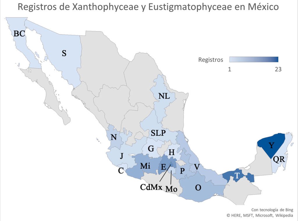
Figura 1. Registros de especies en México. BC: Baja California, C: Colima, CDMX: Ciudad de México, E: Estado de México, G: Guanajuato, H: Hidalgo, J: Jalisco, Mi: Michoacán, Mo: Morelos, N: Nayarit, NL: Nuevo León, O: Oaxaca, P: Puebla, Q: Quintana Roo, SLP: San Luis Potosí, S: Sonora, T: Tabasco, V: Veracruz, Y: Yucatán.
Materiales y métodos
Los cuerpos de agua muestreados en este trabajo corresponden a sitios con registros previos de especies de estas clases (Cantera Oriente, canal El Bordo, lago Huetzalín, presa Ignacio Ramírez) y otras localidades que se agregaron como posibles ambientes en donde podríamos encontrar las especies de interés (presa Requena, lagos Coatetelco, El Rodeo y Atlangatepec). En total, se muestrearon 8 lagos en la región central de México contemplando la Ciudad de México, Estado de México, Hidalgo, Morelos y Tlaxcala (fig. 2, tabla 1).
Tabla 1
Información sobre las localidades y fechas de colecta.
| Estado/ municipio | Cuerpo de agua | Número de localidad | Fecha de colecta | Muestra de herbario |
| Ciudad de México Xochimilco | Huetzalín | 1 | 13 de octubre de 2021 | FCME_CM971 |
| Coyoacán | Mexcalpique | 2 | 19 de octubre de 2021 | FCME_CM972-FCME_CM973 |
| Xochimilco | Canal El Bordo | 3 | 26 de octubre de 2021 | FCME_CM974-FCME_CM977 |
| Estado de México Mayorazgo | Presa Ignacio Ramírez | 4 | 16 de marzo de 2022 | FCME_EDM64-FCME_EDM65 |
| Hidalgo Entre Tepeji del Río de Ocampo y Tula de Allende | Presa Requena | 5 | 20 de marzo de 2023 | FCME_HGO090-FCME_HGO091 |
| Morelos Jojutla | Coatetelco | 6 | 26 de mayo de 2023 | FCME_MOR002 |
| Miacatlán | El Rodeo | 7 | 26 de mayo de 2023 | FCME_MOR003 |
| Tlaxcala Atlangatepec | Atlangatepec | 8 | 23 de junio de 2023 | FCME_TLX001-FCME_TLX002 |
Localidad 1: lago Huetzalín pertenece al Parque Ecológico Xochimilco (PEX), una zona de recuperación ubicada en Xochimilco con una superficie de 1.9 km2 (Tavera et al., 2018). Localidad 2: la Cantera Oriente (CO) área rodeada por una pared de basalto (con una altura de hasta 40 m) que alberga varios cuerpos de agua con una superficie total de 11,906.45 m2 (Lot, 2007), perteneciente a la Reserva Ecológica del Pedregal de San Ángel. Localidad 3: el canal El Bordo es uno de los componentes de la zona chinampera de Xochimilco establecida como área natural protegida desde 1992, inscrita en la lista de humedales de importancia internacional por la Convención Internacional sobre Humedales Ramsar en 2004 (Figueroa et al., 2015). Localidad 4: presa Ignacio Ramírez (municipio Mayorazgo, Estado de México) es el acuífero más importante de la zona pues cuenta con disponibilidad de agua subterránea. Localidad 5: presa Requena (Hidalgo) es indispensable para la regulación de los escurrimientos del río Tula (Ríos, 2009), además de que está contemplada en el programa de ordenamiento ecológico local del municipio de Tepeji del Río de Ocampo desde 2004 (Valdez, 2012). Localidad 6: lago Coatetelco recibe aportes de arroyos del municipio Miacatlán, es un espacio de gran importancia social y económica (Macedonio, 2024). Los lagos Coatetelco y El Rodeo (localidad 7) representan los principales recursos hídricos del estado de Morelos. Ambos están dentro del programa de ordenamiento ecológico con el objetivo de restaurar las funciones ecológicas del sitio y disminuir acciones antropogénicas (Conabio, 2020). Localidad 8: lago Atlangatepec, representa un recurso relevante dentro de su territorio, en Tlaxcala, pues es el más grande y es alimentado por el río Zahuapan, el cual representa un riesgo por la contaminación que presenta por la descarga de material urbano e industrial (López-Segovia et al., 2024).
En cada sitio se filtraron 10 L de agua con una red de fitoplancton (10 µm), este material se concentró en 250 mL y una alícuota de 20 mL se guardó como muestra de herbario y en otro frasco de 200 mL como material de cultivo y observación. El frasco de cultivo se mantuvo en hielo hasta llegar al laboratorio y observar el material vivo. El frasco que se incorporó a las muestras de herbario (FCME) se preservó usando formaldehído al 2.5%. Se tomaron datos de las variables fisicoquímicas: radiación fotosintéticamente activa (PAR, sensores HOBO Penclant Couple MR), temperatura, pH, conductividad, oxígeno disuelto y clorofila a con una sonda multiparamétrica (Hydrolab DS 5 MR).
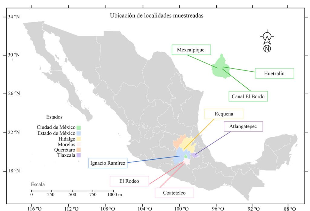
Figura 2. Ubicación de los lagos que se muestrearon en este estudio (Google Earth, 2025).
El cultivo de las especies se realizó en 2 medios de cultivo líquido: bold basal y bristol. El material filtrado se revisó y al identificar especies de interés se continuó con el aislamiento de ejemplares usando un capilar y material de succión. Los cultivos se ubicaron en condiciones de luz y oscuridad (16:8), con un promedio de 3,150 luxes y un intervalo de temperatura de 17-32 °C. Una parte del material de cultivo se procesó para fotografiarlo con microscopía electrónica de barrido. El procedimiento que se realizó usando glutaraldehído fue siguiendo a Takano y Hiroguchi (2005) para su observación. Los equipos utilizados fueron: Jeol JSM-5310LV y Hitachi SU1510.
Se realizaron preparaciones semipermanentes usando el material fijado (2.5%) y gelatina glicerinada (González-González y Novelo, 1986). La observación del material se realizó en un microscopio con contraste interdiferencial (Nikon 80i), para confirmar algunos caracteres morfológicos. Las fotografías se tomaron con una cámara Jenoptik adecuada al microscopio. Las fotografías y láminas se editaron para mejorar el contraste con el programa Photoshop (Adobe Photoshop [versión 26.8.1, 2025]).
En la identificación de las especies, las principales fuentes de consulta fueron: Bourrelly (1952, 1981), Ettl (1978), Ettl y Gärtner (1995); John et al. (2002), Pascher et al. (1925) y Starmach (1968). Y de manera particular se usaron: Bicudo et al. (2006: Characiopsis anabaenae, Chloridella cystiformis, Goniochloris mutica, Isthmochloron lobulatum, Pseudopolyedriopsis skujae, Tribonema minus); Hollerbach (1962: Pseudopolydriopsis skujae); Islam e Irfanullah (2001: Tetraplektron torsum); Krienitz et al. (1993: Pseudogoniochloris tripus); Krienitz et al. (2000: Nannochloropsis limnetica); Novelo et al. (2009: Botrydiopsis arhiza y Chloridella cystiformis).
Los datos de distribución geográfica y ambiental se obtuvieron de bdLACET (Novelo y Tavera, 2025), AlgaeBase (Guiry y Guiry 2025) y GBIF (Global Biodiversity Information Facility, 2025). El análisis de similitud con el índice de Jaccard se realizó con el programa PAST versión 4.17 (Hammer et al., 2001), construyendo una matriz de presencia y ausencia de las especies en los 8 sitios (con los parámetros establecidos en el programa). El análisis de agrupamiento (con distancia euclidiana, con el algoritmo UPGMA) se realizó utilizando los datos ambientales medidos en cada sitio de muestreo: temperatura (°C), pH, conductividad (µS), oxígeno disuelto (mg/L) y concentración de clorofila a (µg/L) (se realizó con los parámetros establecidos en el programa), los datos se transformaron con logaritmo base 10.
Resultados
Los datos de variables ambientales obtenidos en campo de los 8 lagos se presentan en la tabla 2, así como también la distribución de las especies por sitio y registro previos en México. El análisis de similitud con el índice de Jaccard se muestra en la tabla 3. Los valores obtenidos nos indican valores bajos de similitud en relación con las especies distribuidas en los sitios. Los valores obtenidos están en un intervalo de 0 a 0.33.
El agrupamiento de los sitios se representa en la figura 3. Los grupos que se formaron en el análisis son 3. El primer grupo (con los sitios más cercanos) es el que se representa con los números 2, 4 y 8, que corresponden a los sitios Mexcalpique (2), presa Ignacio Ramírez (4) y Atlangatepec (8); el siguiente grupo, con los sitios 1 (Huetzalín) y 7 (El Rodeo), y el último grupo con los sitios 5 (presa Requena), 6 (Coatetelco) y 3 (Bordo). En las muestras se identificaron en total 18 especies en la región central de México y corresponden a las 2 clases, de acuerdo con bases de datos actualizadas (bdLACET y AlgaeBase), 10 de ellas se clasifican en la clase Xanthophyceae y 8 en la clase Eustigmatophyceae.
Xanthophyceae P. Allorge ex F.E. Fritsch
Rhizochloridales Pascher
Stipitococcaceae Ettl
Stipitococcus W. et G. S. West
Stipitococcus capensis Prescott, 1937 (fig. 4)
Células solitarias, lorica con forma elipsoidal-ovoide ligeramente alargada, en la base presenta un pedúnculo corto que se adhiere a otras algas (encontradas sobre células de Stephanocyclus meneghinianus). Célula elipsoidal con un plastidio lobulado. Las células miden 7.8-9.7 µm de largo y 4.0-6.3 µm de ancho, con un pedúnculo corto de hasta 2.0 µm.
Distribución en México: Oaxaca, Ciudad de México (Xochimilco). Mundial: España, EUA e India.
Ambientes: estanques, lagos.
Formas de vida: planctónica, epífita y metafítica.
Referencias: Bourrelly, 1981; Ettl, 1978; Pascher et al., 1925; Starmach, 1968.
Tabla 2
Valores de variables fisicoquímicas obtenidos en campo en los 8 sitios de muestreo: 1) Huetzalín – PEX; 2) Mexcalpique – Cantera Oriente; 3) canal El Bordo – Xochimilco; 4) presa Ignacio Ramírez; 5) presa Requena; 6) Coatetelco; 7) El Rodeo; 8) Atlangatepec.
| Variable y especie/ sitio | 1 | 2 | 3 | 4 | 5 | 6 | 7 | 8 | Distribución en México |
| Temperatura (°C) | 24 | 16.4 | 15.4 | 24 | 19.4 | 32.8 | 29.9 | 26.1 | |
| pH | 8.7 | 8.1 | 6.9 | 9.1 | 9.5 | 8 | 8.3 | 9.2 | |
| Conductividad (µS) | 0 | 364 | 932 | 291 | 826 | 878 | 168 | 401 | |
| DO (mg/L) | 6.19 | 7.12 | 0.22 | 10.6 | 5.26 | 5.06 | 5.78 | 8.25 | |
| Clorofila a (µg/L) | 0.96 | 59.05 | 3.75 | 29.94 | 6.94 | 6.31 | 41.1 | 26.97 | |
| Stipitococcus capensis | x | CdMx, Oaxaca | |||||||
| Chloridella cystiformis | x | x | CdMx, Tabasco | ||||||
| Ellipsoidion oocystoides | x | Nuevo Registro | |||||||
| Monodus guttula | x | Nuevo Registro | |||||||
| Tetraplektron torsum | x | Michoacán, Yucatán. | |||||||
| Pseudogoniochloris tripus | x | x | Tabasco, Nayarit. | ||||||
| Isthmochloron lobulatum | x | Tabasco, Nayarit. | |||||||
| Pseudopolydriopsis skujae | x | Nuevo registro | |||||||
| Botrydiopsis arhiza | x | Jalisco | |||||||
| Tribonema minus | x | x | CdMx | ||||||
| Nannochloropsis limnetica | x | Nuevo registro | |||||||
| Characiopsis anabaenae | x | Nuevo registro | |||||||
| Goniochloris mutica | x | x | x | CdMx, Tabasco, Nayarit. | |||||
| G. iyengarii | x | x | x | Tabasco | |||||
| Pseudostaurastrum limneticum | x | Estado de México | |||||||
| Tetraedriella acuta | x | Tabasco | |||||||
| Trachydiscus minutus | x | Tabasco | |||||||
| T. lenticularis | x | Nuevo registro |
Tabla 3
Valores de similitud (índice de Jaccard).
| 1 | 2 | 3 | 4 | 5 | 6 | 7 | 8 | |
| 1 | 1 | 0.16666667 | 0.14285714 | 0 | 0 | 0 | 0 | 0.14285714 |
| 2 | 0.16666667 | 1 | 0 | 0 | 0 | 0.14285714 | 0 | 0 |
| 3 | 0.14285714 | 0 | 1 | 0 | 0 | 0.125 | 0 | 0.33333333 |
| 4 | 0 | 0 | 0 | 1 | 0 | 0 | 0 | 0 |
| 5 | 0 | 0 | 0 | 0 | 1 | 0 | 0 | 0 |
| 6 | 0 | 0.14285714 | 0.125 | 0 | 0 | 1 | 0 | 0.125 |
| 7 | 0 | 0 | 0 | 0 | 0 | 0 | 1 | 0 |
| 8 | 0.14285714 | 0 | 0.33333333 | 0 | 0 | 0.125 | 0 | 1 |
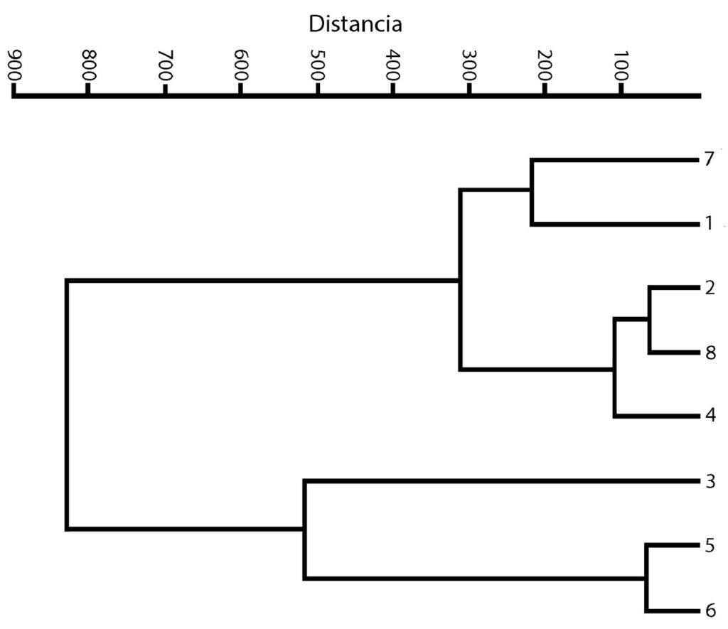
Figura 3. Dendrograma. Agrupamiento de los 8 sitios recolectados.
Mischococcales F.E. Fritsch
Pleurochloridaceae Pascher
Género Chloridella Pascher
Chloridella cystiformis Pascher, 1937 (figs. 5, 6)
Células solitarias, generalmente esféricas con pared lisa a veces amarillenta y gruesa, 2-4 plastidios discoidales, parietales. Las células miden 4.8-9.3 µm de diámetro.
Distribución en México: Ciudad de México (Cantera Oriente, PEX), Tabasco. Mundial: Alemania, Brasil, España, Eslovaquia, EUA, Polonia, República Checa, Rusia y Ucrania.
Ambientes: estanques y lagos.
Forma de vida: metafítica.
Referencias: Bicudo et al., 2006; Bourrelly, 1981; Ettl, 1978; Novelo et al., 2009; Pascher et al., 1925.
Nota: se encuentra en grandes cantidades en cuerpos de agua con un alto contenido de hierro y valores ácidos de pH (Ettl, 1978).
Ellipsoidion Pascher
Ellipsoidion oocystoides Pascher, 1938 (figs. 7, 8)
Células elipsoidales con extremos redondeados, generalmente 1.5 veces más largas que anchas, pared celular lisa, un plastidio laminar parietal. Las células miden 5.8-6.5 µm de largo y 2.9-3.8 µm de ancho.
Distribución en México: primer registro en Estado de México (presa Ignacio Ramírez) y México. Mundial: Alemania, Australia, Austria, Brasil, Corea del Norte, Eslovaquia, España, Islandia, Japón, República Checa, Rumania, Rusia y Tayikistán.
Ambientes: lagos y suelos.
Formas de vida: metafítica, edáfica.
Nota: común en aguas y suelos ácidos (Ettl, 1978).
Referencias: Bourrelly 1981; Ettl, 1978; Starmach, 1968.
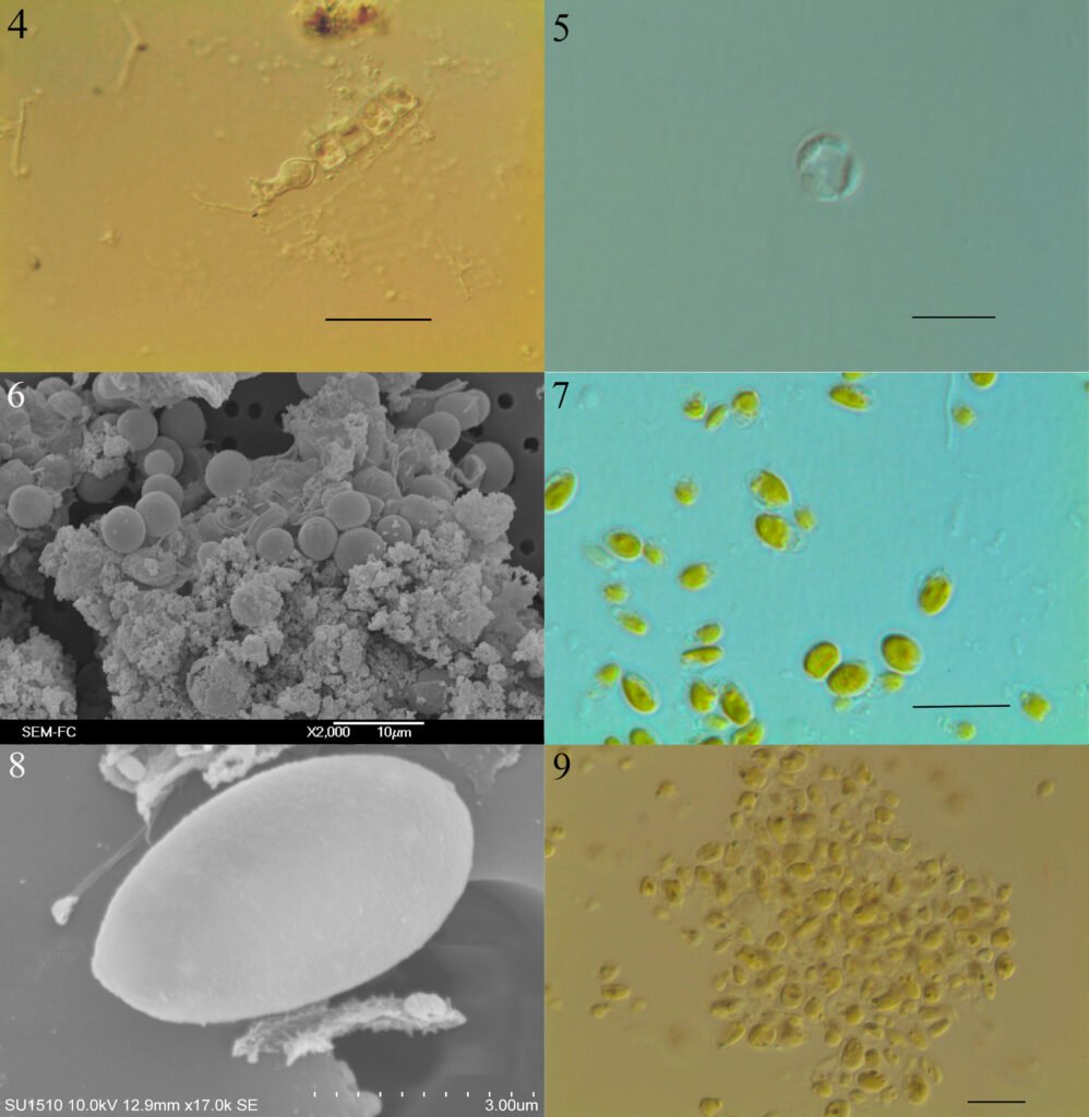
Figuras 4-9. 4, Stipitococcus capensis; 5, Chloridella cystiformis; 6, C. cystiformis (MEB); 7, Ellipsoidion oocystoides; 8, E. oocystoides (MEB); 9, Monodus guttula (cultivo). Barra = 10 µm.
Monodus Chodat
Monodus guttula Pascher, 1938 (figs. 9-11)
Células solitarias globosas u ovadas, puntiagudas en un extremo, ligeramente curvas, pared lisa y delgada, un plastidio laminar parietal. Las células miden 3.8-4.9 µm de largo y 2.2-2.9 µm de ancho.
Distribución en México: primer registro en Ciudad de México (Cantera Oriente). Mundial: Alemania, Bulgaria, Eslovaquia, España, Islas Shetland del Sur, Moldavia, República Checa, Rumania y Rusia.
Ambientes: lagos.
Formas de vida: metafítica.
Nota: se encuentran en lugares húmedos y zanjas en las cordilleras entre Alemania y la República Checa (Ettl, 1978).
Referencia: Bourrelly, 1981; Ettl, 1978; Pascher et al., 1925, Starmach, 1968.
Tetraplektron Fott
Tetraplektron torsum (Turner) Dedusenko Ščegoleva, 1962 (fig. 12)
Células solitarias, tetraédricas aplanadas, cada lado termina en una espina, un lado enmascara otro, pared celular lisa y gruesa, varios plastidios discoidales. Las células miden 44.2- 46.6 µm de largo y 22.1-22.9 µm de ancho.
Distribución en México: Morelos (El Rodeo), Michoacán y Yucatán. Mundial: Alemania, Australia, Bangladesh, Brasil, Costa de Marfil, EUA, Italia, Myanmar, Países Bajos, Paraguay, Suecia y Ucrania.
Ambientes: lagos.
Formas de vida: Planctónica, perifítica y metafítica.
Referencias: Bourrelly, 1981; Ettl, 1978; Islam e Irfanullah, 2001; John et al., 2002; Starmach, 1968.
Pseudogoniochloris (Pascher) Krienitz, Hegewald, Reymond et Peschke
Pseudogoniochloris tripus (Pascher) Krienitz, Hegewald, Reymonds et Peschke, 1993 (fig. 13).
Células triangulares irregulares (ligeramente torcidas) con bordes agudos, lados cóncavos, pared celular lisa o ligeramente ornamentada, 3-5 plastidios (puede haber más) discoidales, parietales. Las células miden 19.5-28.3 µm por lado.
Distribución en México: Ciudad de México (Xochimilco), Tlaxcala (Atlangatepec), Tabasco y Nayarit. Mundial: Alemania, Argentina, Australia, Austria, Bangladesh, Bélgica, Bielorrusia, Botsuana, Brasil, China, Eslovaquia, EUA, Estonia, Francia, India, Irlanda, Israel, Japón, Países Bajos, Paraguay, Reino Unido, República Checa, Rumania, Rusia, Suecia, Sudáfrica, Turquía y Ucrania.
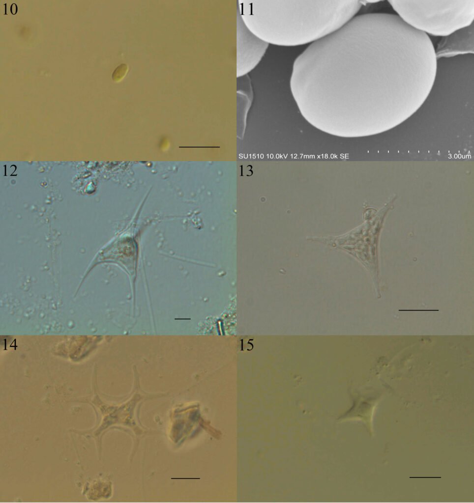
Figuras 10-15. 10, Monodus guttula (campo); 11, M. guttula (MEB); 12, Tetraplektron torsum; 13, Pseudogoniochloris tripus; 14: Isthmochloron lobulatum; 15, Pseudopolyedriopsis skujae. Barra = 10 µm.
Ambientes: lagos.
Formas de vida: planctónica y metafítica.
Referencias: Bicudo et al., 2006; Bourrelly 1952, 1981; Ettl, 1978; Krienitz et al., 1993; Starmach, 1968.
Isthmochloron Skuja
Isthmochloron lobulatum (Nägeli) Skuja, 1948 (fig. 14)
Células solitarias, cuadrangulares con lados cóncavos que se dividen dicotómicamente al final, pared celular lisa, varios plastidios discoidales, parietales. Las células miden 7.8-11.7 en la parte central, sin brazos y miden 28.2-34.7 µm de cada lado con brazos.
Distribución en México: Morelos (Coatetelco), Tabasco y Nayarit. Mundial: en los 5 continentes.
Ambientes: lagos.
Formas de vida: metafítica y planctónica.
Referencias: Bicudo et al., 2006; Bourrelly 1952, 1981; Ettl, 1978; John et al., 2002; Starmach, 1968.
Pseudopolyedriopsis Gollerbach
Pseudopolyedriopsis skujae Gollerbach, 1962 (fig. 15)
Células solitarias, aplanadas con 5 proyecciones angulosas, pared celular gruesa, ornamentación muy fina, varios plastidios discoidales parietales. Las células miden 9.3-17.1 µm de cada lado. Presentan 2-4 espinas de 13.2-18.6 µm en cada proyección.
Distribución en México: primer registro en México, Ciudad de México (Xochimilco). Mundial: Alemania, Australia, Bélgica, Bielorrusia, Brasil, EUA, Estonia, Francia, Países Bajos y Suecia.
Ambientes: lagos.
Formas de vida: metafítica.
Nota: los ejemplares observados sólo presentan espinas en campo, no en los cultivos.
Referencias: Bicudo et al., 2006; Bourrelly, 1981; Ettl, 1978; Hollerbach, 1962; Starmach, 1968.
Botrydiopsidaceae D.J. Hibberd
Botrydiopsis Borzì
Botrydiopsis arhiza Borzì, 1895 (figs. 16-18)
Células esféricas, generalmente en grupos unidos por mucílago incoloro o pardo, pared celular gruesa a muy gruesa, varios plastidios discoidales o rectangulares. Las células miden 13.6-23.5 µm de diámetro.
Distribución en México: Ciudad de México (Cantera Oriente), Jalisco. Mundial: EUA, Japón, India, Países Bajos, Portugal, Reino Unido, Rusia, Suecia y Ucrania.
Ambientes: suelos, lagos, arenas y charcos.
Formas de vida: edáfica, planctónica y metafítica.
Referencias: Bourrelly, 1981; Ettl, 1978; John et al., 2002; Novelo et al., 2009; Pascher et al., 1925; Starmach, 1968.
Tribonematales Pascher
Tribonemataceae Pascher
Tribonema Derbès et Solier
Tribonema minus Wille (Hazen), 1902 (fig. 19)
Filamentos uniseriados, cortos, rectos o curvos. Células cilíndricas con septos definidos y sin constricción, pared celular lisa, 2 a 3 plastidios laminares, parietales. Las células miden 4.4-5.9 µm de ancho y 17.5-26.3 µm de largo.
Distribución en México: Ciudad de México (Cantera Oriente). Mundial: Alemania, Arabia Saudita, Austria, Brasil, Canadá, España, EUA, Estonia, Grecia, Hungría, Nigeria, Países Bajos, Polonia, Reino Unido, Suecia, Ucrania y Uzbekistán.
Ambientes: ríos, arroyos, lagos, humedales, charcos, estanques, embalses y turberas.
Formas de vida: bentónica, metafítica, planctónica.
Referencias: Bicudo et al., 2006; Bourrelly, 1981; Ettl, 1978; Ettl y Gärtner, 1995; John et al., 2002; Starmach, 1968.
Eustigmatophyceae D.J. Hibberd et Leedale
Eustigmatales D.J. Hibberd
Monodopsidaceae D.J. Hibberd
Nannochloropsis D.J. Hibberd
Nannochloropsis limnetica Krienitz, Hepperle, Stich et Weiler, 2000 (figs. 20, 21)
Células esféricas, ovaladas o en forma de gota, pared celular lisa, 1-2 plastidios discoidales, parietales. Las células miden 3.1-3.4 µm de diámetro.
Distribución en México: Ciudad de México (Cantera Oriente). Mundial: Alemania, Canadá, China, Curazao, Dinamarca, Eslovenia, EUA, Finlandia, Francia, Grecia, Israel, Noruega, Polonia, Reino Unido, Rusia y Suecia.
Ambientes: lagos.
Forma de vida: metafítica.
Referencias: Krienitz et al., 2000.
Characiopsidaceae Pascher
Characiopsis Borzì
Characiopsis anabaenae Pascher, 1938 (figs. 22, 23)
Células solitarias, pequeñas, fusiformes, con un lado más convexo que el otro, terminación aguda de un extremo en donde se encuentra el disco basal, pared celular lisa, 2 plastidios laminares. Las células miden 10.7-18.6 µm de largo y 2.0-5.9 µm de ancho.
Distribución en México: primer registro en México, Hidalgo (Presa Requena). Mundial: Afganistán, Alemania, Brasil, Países Bajos, Portugal, Rumania, Rusia y Ucrania.
Ambientes: lagos.
Forma de vida: metafítica.
Referencias: Bicudo et al., 2006; Bourrelly, 1981; Ettl, 1978; Ettl y Gärtner, 1995; Starmach, 1968.
Goniochloridales K.P. Fawley, M. Eliás et M.W. Fawley
Goniochloridaceae
Goniochloris Pascher
Goniochloris mutica (A. Braun) Fott, 1960 (fig. 24)
Células solitarias, triangulares regulares con bordes redondeados, lados cóncavos, pared celular ornamentada con pequeñas verrugas, 2-3 plastidios discoidales. Las células miden 5.8-9.8 µm de cada lado.
Distribución en México: Ciudad de México (Xochimilco), Tlaxcala (Atlangatepec), Tabasco y Nayarit. Mundial: Alemania, Australia, Argentina, Bangladesh, Bélgica, Bielorrusia, Botswana, Brasil, Burindi, Canadá, China, Costa de Marfil, Eslovaquia, España, EUA, Estonia, Francia, India, Irak, Irán, Israel, Italia, Niger, Nueva Zelanda, Países Bajos, Portugal, Reino Unido, República Checa, Rumania, Rusia, Sudán, Suecia, Taiwán, Tayjikistán, Turquía y Ucrania.
Ambientes: humedales y lagos.
Formas de vida: planctónica y metafítica.
Referencias: Bicudo et al., 2006; Bourrelly 1952, 1981; Ettl, 1978; John et al., 2002; Starmach, 1968.
Goniochloris iyengarii (Ramanathan) Ettl, 1977 (fig. 25)
Células solitarias, triangulares con terminaciones agudas, lados ligeramente cóncavos, pared celular gruesa con ornamentación escrobiculada, varios plastidios discoidales, parietales. Las células miden 22.3-26.4 µm de cada lado.
Distribución en México: Ciudad de México (Xochimilco), Morelos (Coatetelco), Tlaxcala (Atlangatepec), Tabasco. Mundial: Alemania, Brasil, Francia (Guadaloupe), India y Países Bajos.
Ambientes: charcos y lagos.
Formas de vida: metafítica.
Referencias: Bourrelly 1981; Ettl, 1978; John et al., 2002; Starmach, 1968.
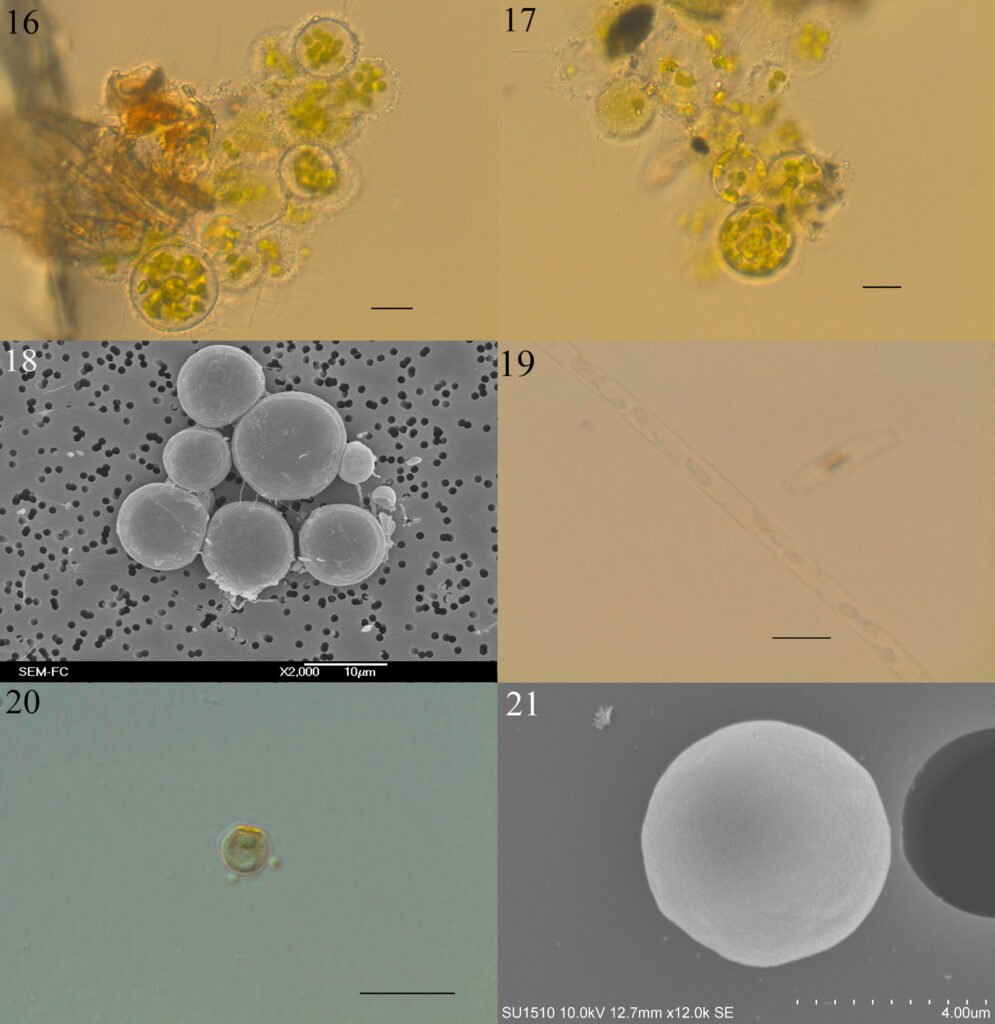
Figuras 16-21. 16, Botrydiopsis arhiza (campo); 17, B. arhiza (cultivo); 18, B. arhiza (MEB); 19, Tribonema minus; 20, Nannochloropsis limnetica; 21, N. limnetica (MEB). Barra = 10 µm.
Pseudostaurastrum Chodat
Pseudostaurastrum limneticum (Borge) Guiry, 2021 (fig. 26)
Células solitarias, tetraédricas con cuerpo central ligeramente amplio que termina en 4 brazos radiados, bifurcados en los extremos, pared celular lisa y gruesa, varios plastidios discoidales y parietales. Las células miden 29.3-34.9 µm de cada lado.
Distribución en México: Tlaxcala (Atlangatepec) y Estado de México. Mundial: Alemania, Argentina, Australia, Bangladesh, Bioelorrusia, Brasil, Canadá, China, Cuba, España, EUA, Estonia, India, Irak, Irlanda, Israel, Japón, Latvia, Mianmar, Nueva Zelanda, Países Bajos, Paquistán, Portugal, Reino Unido, República Checa, Rumania, Rusia, Sudán, Suecia, Taiwán, Turquía, Ucrania y Venezuela.
Ambientes: lagos.
Formas de vida: planctónica y metafítica.
Referencias: Bourrelly, 1981; Ettl, 1978; John et al., 2002; Starmach, 1968.
Tetraedriella Pascher
Tetraedriella acuta Pascher, 1930 (fig. 27)
Células solitarias, tetraédricas, con lados convexos y bordes ligeramente afilados, pared celular gruesa ornamentada en forma de panal con bordes aún más engrosados, 4 plastidios discoidales. Las células miden 10.3-13.7 µm de cada lado.
Distribución en México: Tabasco y Ciudad de México (Xochimilco). Mundial: Alemania, Brasil, Bulgaria, Costa de Marfil, España, Estonia, Francia, Países Bajos y República Checa.
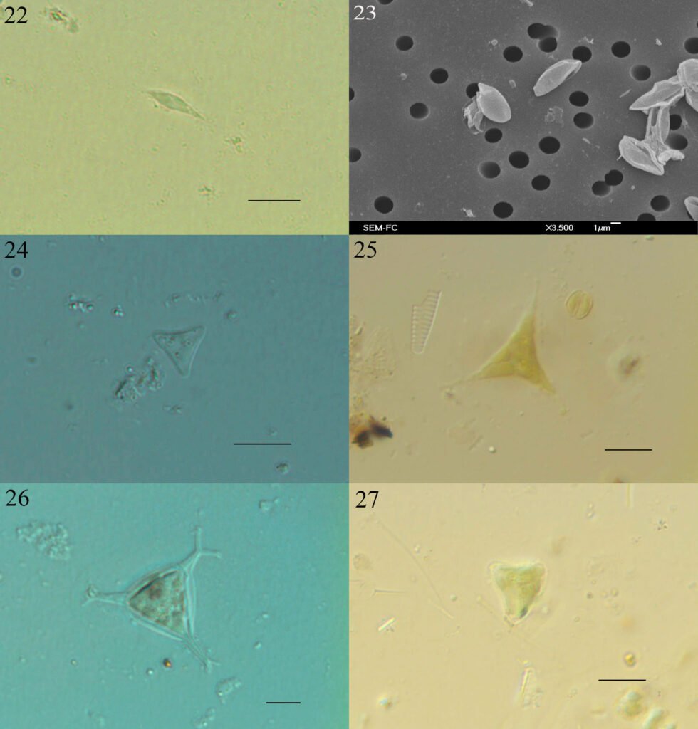
Figuras 22-27. 22, Characiopsis anabaenae; 23, C. anabaenae (MEB); 24, Goniochloris mutica, 25; G. iyengarii, 26; Pseudostaurastrum limneticum, 27; Tetraedriella acuta. Barra = 10 µm.
Ambientes: lagos.
Formas de vida: metafítica.
Nota: valores ácidos de pH (Ettl, 1978).
Referencias; Bourrelly, 1981; Ettl, 1978; Starmach, 1968.
Trachydiscus Ettl
Trachydiscus minutus (Bourrelly) Ettl, 1964 (fig. 28)
Células solitarias, pentagonales redondeadas en los ángulos, pared celular delicadamente ornamentada, 4 a 5 plastidios discoidales. Las células miden 6.8-9.8 µm de diámetro.
Distribución en México: Tlaxcala (Atlangatepec) y Tabasco. Mundial: Argentina, Australia, Bélgica, Bulgaria, Canadá, China, Colombia, Corea del Sur, EUA, Finlandia, Francia, Grecia, Polonia, Reino Unido, República Checa, Suecia, Turquía y Ucrania.
Ambientes: estanques, lagos.
Formas de vida: planctónica, metafítica.
Referencias: Bourrelly 1952, 1981; Ettl, 1978; Starmach, 1968.
Trachydiscus lenticularis Ettl, 1964 (fig. 29)
Células solitarias, lenticulares, biconvexas, pared celular ornamentada con verrugas pequeñas, 3 plastos discoidales. Las células miden 8.6-9.8 µm de diámetro.
Distribución en México: primer registro en México, Tlaxcala (Atlangatepec). Mundial: Alemania, Bélgica, España, Francia, Irlanda, Países Bajos, República Checa y Reino Unido.
Ambientes: estanques, lagos.
Formas de vida: planctónica, metafítica.
Referencias: Bourrelly 1952, 1981; Ettl, 1978; Starmach, 1968.
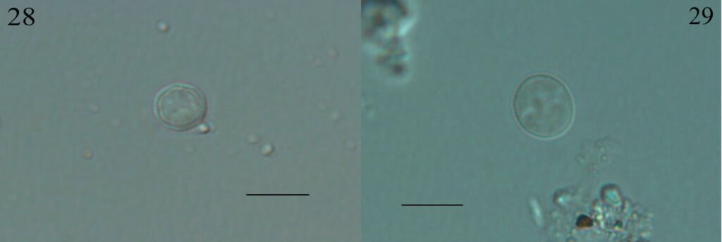
Figuras 28-29. 28, Trachydiscus minutus; 29, T. lenticularis. Barra = 10 µm.
Discusión
Los registros previos de especies de las Xanthophyceae y Eustigmatophyceae en los sitios seleccionados de la región central de México se muestran en la tabla 4. En la Ciudad de México, de las 8 especies registradas, confirmamos la presencia actual de 3 de ellas, Botrydiopsis arhiza, Chloridella cystiformis y Tribonema minus. B. arhiza ha sido reportada en 3 trabajos, el primero, en el catálogo de algas de Ortega (1984); el segundo, como un taxón a comparar que se encuentra por periodos en distintos cuerpos de agua siendo parte de distintas comunidades: fitoplancton, metafiton y perifiton (Novelo et al., 2009); nosotros la encontramos en un cuerpo de agua estancado dentro de la Cantera Oriente, en octubre, formando un crecimiento evidente en la superficie casi monoespecífico de fitoplancton; el tercer registro, menciona la especie como parte de las algas de la cuenca de la ciudad (Figueroa, 2009). Previamente registrada en EUA, varios países de Europa, Rusia, Japón e India.
C. cystiformis fue registrada por primera vez en la Cantera Oriente como una especie de ambientes templados y ácidos (Novelo et al., 2009); en este trabajo se registra en el mismo sitio, lago Mexcalpique, en el metafiton, corroborando su presencia y crecimiento en la misma comunidad, sin embargo, las condiciones no son similares pues los valores de pH no son ácidos (como se ha registrado previamente en localidades de Europa), sino básicos en el sitio donde la observamos (tabla 2), además también la encontramos en el lago Huetzalín (PEX) y en sitios con valores de pH básico.
En el caso de T. minus, se ha reportado en más ocasiones, ejemplo de la desigualdad de trabajos que registran especies de mayor talla, en este caso filamentosas que especies unicelulares, en canales de Xochimilco (Figueroa, 2009; Figueroa et al., 2015; Flores, 1980; González-Barrera, 1991) y en Cantera Oriente (Ponce et al., 2019). Esta especie ha sido registrada previamente en localidades frías de Europa, pero también en templadas o cálidas como EUA y Brasil.
Como nuevos registros de la Ciudad de México se tienen a Monodus guttula y Pseudopolydriopsis skujae. La primera descrita para el lago Mexcalpique en la Cantera Oriente, con registros previos en Europa y la segunda para el canal El Bordo en Xochimilco, presente en Europa y en Brasil. Por último, algunos registros que no estaban reportados en las zonas seleccionadas, pero sí en el país son: Stipitococcus capensis, en el Bordo, en Xochimilco, con registros en Europa, Norteamérica y Asia, en México se había descrito en Oaxaca. Pseudogoniochloris tripus, previamente registrado en Tabasco (Agredano, 2019; Mireles, 2019; Pedraza, 2020) y Nayarit (Ochoa, 2023), de amplia distribución mundial, se encontró en el canal Bordo; Nannochloropsis limnetica, se registra en el lago Mexcalpique, es una especie que ha proliferado en muchos ambientes en el mundo, ahora como primer registro en Cantera Oriente. En el lago Huetzalín, se observaron en el metafiton a Goniochloris mutica, con registros previos en los canales de Xochimilco (Tavera y Diez, 2009), Tabasco (Mireles, 2019) y Nayarit (Ochoa, 2023) y amplia distribución mundial; así como a G. iyengarii con registro anterior en Tabasco (Mireles, 2019) y con poca distribución mundial; y a Tetraedriella acuta, con registro previo en Tabasco (Mireles, 2019), en Europa y Brasil.
Tabla 4
Especies registradas previamente en las zonas de la región central de México.
| Estado (número de especies registradas) | Especie | Referencias |
| CdMx (8) | Botrydiopsis arhiza Borzì | Ortega, 1984 Novelo et al., 2009 Figueroa, 2009 |
| Characiopsis naegelii (A. Braun) Lemmermann | Ortega, 1984, Figueroa, 2009 | |
| Tabla 4. Continúa | ||
| Estado (número de especies registradas) | Especie | Referencias |
| Chloridella cystiformis Pascher | Novelo et al., 2009 | |
| Dichotomosiphon tuberosus (A. Braun) Ernest | Figueroa, 2009 Cantoral et al., 1999 | |
| Ducelleria chodatii (Ducellier) Teiling | Godínez-Ortega et al., 2017 | |
| Gloeobotrys limneticus (G.M. Smith) Pascher | Ortega, 1984 Figueroa, 2009 | |
| Ophiocytium capitatum Wolle | Figueroa et al., 2015 Figueroa, 2009 Flores-Granados, 1980 | |
| Tribonema minus (Wille) Hazen | Figueroa, 2009 Flores-Granados, 1980 González-Barrera, 1991 Figueroa et al., 2015 Ponce et al., 2019 | |
| Estado de México (10) | Bumilleriopsis brevis (Gerenck) Printz | Moreno y Palacios, 1987 |
| Characiopsis longipes (Rabenhorst) Borzì | Banderas-Tarabay, 1994 Banderas-Tarabay, 1997 | |
| Chlorocloster pyreniger Pascher | Favari et al., 2002 | |
| Ophiocytium capitatum Wolle | Chávez et al., 2005 | |
| O. cochleare (Eichwald) A. Braun | Mendoza, 1985 Ortega, 1984 Chávez et al., 2005 Figueroa, 2009 | |
| O. lagerheimii Lemmermann | Chávez et al., 2005 | |
| O. majus Nägeli | Chávez et al., 2005 | |
| O. parvulum (Perty) A. Braun | Zariñana-Leguízamo, 1997 Chávez et al., 2005 | |
| Vaucheria bursata (O.F. Müller) C. Agardh | Bojorge et al., 2010 Ramírez, 2010 Rodríguez-Flores, 2014 Rodríguez-Flores y Carmona, 2018 | |
| V. geminata (Vaucher) de Candolle | Ortega, 1984 Mendoza, 1985 Figueroa, 2009 Garduño-Solórzano et al., 2009 Ceballos et al., 2009 | |
| Morelos (3) | Ophiocytium capitatum Wolle | Flórez, 2011 |
| Tribonema bombycinum (C.A. Agardh) Derbés et Solier | García-Rodríguez y Tavera, 1998 Quiroz-Castelán et al., 2007 García-Rodríguez, 2004 | |
| Vaucheria sessilis f. clavata (De Candolle) Heering | Valadez-Cruz et al., 1996 Valadez-Cruz, 1998 | |
| Ducelleria chodatii (Ducellier) Teiling | Godínez-Ortega et al., 2017 |
De los registros en el Estado de México (10) no corroboramos ninguna de las especies de la tabla 4. Favari et al. (2002) reportan para la presa Ignacio Ramírez a Chlorocloster pyreniger, en este estudio con la observación de material de campo tanto vivo como fijado, no se corroboró su presencia. En el caso de Ellipsoidion oocystoides, se registra por primera vez en el país, con reportes previos en zona templada de Europa, Japón y zonas tropicales como Brasil, Australia y Nueva Zelanda.
Para la presa Requena, Hidalgo, no existían registros publicados sobre este grupo de algas, en la revisión de las muestras de este estudio encontramos a Characiopsis anabaenae, primer registro para México, previamente descrito en Europa, Asia y Brasil.
En Morelos, los 4 registros previos de algas doradas no se corroboraron, incluso en el sitio que visitamos, El Rodeo. En el lago Coatetelco identificamos Goniochloris mutica (mencionada para Huetzalín) e Isthmochloron lobulatum que ya tenía registros previos en Tabasco (Mireles, 2019) y Nayarit (Ochoa, 2023) y con amplia distribución mundial. En el lago El Rodeo, también identificamos a I. lobulatum y Tetraplektron torsum, esta última se había registrado en Michoacán (Martínez, 2016) y Yucatán (López-Adrián y Catzim, 2010), en parte de Europa, Sudamérica y Asia. Pseudostaurastrum limneticum, previamente registrada en el Estado de México (Jiménez, 2010) y con amplia distribución mundial.
En Tlaxcala, en el lago Atlangatepec, identificamos 6 especies: Pseudogoniochloris tripus, Goniochloris mutica, G. iyengarii, Pseudostaurastrum limneticum, Trachydiscus minutus y T. lenticularis. T. minutus, con registro previo en Tabasco (Pedraza, 2020), Europa y Argentina, muy escasos son los trabajos con esta especie. Mientras, que T. lenticularis, es primer registro en México y solo se ha reportado en ambientes fríos de Europa, Alemania, Bélgica, España, Francia, Irlanda, Países Bajos, República Checa y Reino Unido (Ettl, 1978; Starmach, 1968).
En relación con los sitios de muestreo y las variables ambientales, el dendrograma obtenido muestra que los sitios más parecidos son: Mexcalpique, presa Ignacio Ramírez y Atlangatepec (localidades 2, 4 y 8, respectivamente), esto resulta así pues los valores ambientales son cercanos en 3 variables, conductividad, oxígeno disuelto y concentración de clorofila a. Los sitios: Huetzalín y El Rodeo (1 y 7, respectivamente) presentan valores cercanos de pH y de oxígeno disuelto. Finalmente, el último grupo, Bordo, presa Requena y Coatetelco (3, 5 y 6 respectivamente), presentan valores cercanos de conductividad y de concentración de clorofila a.
La distribución de las especies utilizando una matriz de presencia/ausencia y aplicando el índice de Jaccard, dio como resultado valores entre 0 y 0.33, estos valores indican una similitud de especies nula o baja entre los sitios (Magurran, 2004). Huetzalín (1) muestra valores 0 con la presa Ignacio Ramírez (4), Presa Requena (5), Coatetelco (6) y El Rodeo (7), un valor de 0.14286 con los lagos El Bordo (3) y Atlangatepec (8) y un valor de 0.167 con Mexcalpique, esto indica una similitud bastante baja, pues solo comparten una especie (Goniochloris mutica) y la mayoría de las especies son diferentes entre sitios. Los valores 0, nos indican que los elementos son 100% diferentes, mientras que en los otros sitios son casi 90% diferentes. Los sitios que muestran los valores más altos (0.334) son El Bordo (3) y Atlangatepec (8), esto es debido a que comparten la presencia de 3 especies (Pseudogoniochloris tripus, Goniochloris mutica y Goniochloris iyengarii). La presencia de especies en cada sitio prácticamente es única, esto se explica por la variación en las condiciones ambientales que pueden limitar el crecimiento de algunas especies y la distancia entre los sitios es lo suficiente para no compartir especies (Magurran, 2004).
Se esperaba que los grupos que se formaron en el dendrograma coincidieran con los sitios con más similitud con la presencia de especies, sin embargo, no ocurrió, lo que nos indica que son conjuntos casi únicos (Real y Vargas, 1996).
Todas las algas son un reto en su identificación, las algas doradas presentadas en este trabajo son un ejemplo de la diversidad que aún desconocemos en distintos sitios del país, seguir estudiando la flora dorada es indispensable en el avance de una solución taxonómica, en un contexto integral.
Agradecimientos
Al Posgrado en Ciencias del Mar y Limnología, UNAM, por los estudios dirigidos a la obtención del grado de Doctor. Al apoyo recibido de Conahcyt (beca con clave 2020-000026-02NACF). A Guadalupe Vidal Gaona por su apoyo en el laboratorio y en campo. A Beatriz Lira Hernández por su apoyo en campo. A Silvia Espinosa Matías de la Facultad de Ciencias por el procesamiento de muestras y obtención de imágenes con el microscopio electrónico de barrido Jeol JSM-5310LV. A María Berenit Mendoza Garfias del Laboratorio Nacional de Biodiversidad del Instituto de Biología por su servicio en el procesamiento de muestra y obtención de imágenes con el microscopio electrónico de barrido Hitachi SU1510. A los revisores, que nos dieron sugerencias para mejorar el manuscrito.
Referencias
Adrián-Serrano, J. (2024). Estudio de la biodiversidad fitoplanctónica del Canal Japón, Xochimilco, México D. F. (Tesis). Facultad de Ciencias, Universidad Nacional Autónoma de México. Ciudad de México.
Agredano, Z. O. (2019). Ficoflora de la laguna El Camarón en Villahermosa, Tabasco, México (Tesis). Facultad de Ciencias, Universidad Nacional Autónoma de México. Ciudad de México.
Aguirre-Cavazos, D. E., Moreno-Limón, S. y Salcedo-Martínez, S. M. (2018). Especies de algas de ríos de Nuevo León, México. Nuevos registros para el estado. Polibotánica, 46, 1–25. https://doi.org/10.18387/polibotanica.46.1
Alcocer, J. y Escobar-Briones, E. (1992). The aquatic biota of the now extinct lacustrine complex of Mexico basin. Freshwater forum, 2, 171–183.
Alvarado-Villanueva, R. (2003). Dinámica estacional y circadiana del fitoplancton en el Lago Zirahuén, Michoacán, México (Tesis de maestría). Facultad de Biología, Universidad Michoacana de San Nicolás de Hidalgo. Morelia.
Amateco-Rivero, F. S. (2011). Composición del fitoplancton del lago de Catemaco, Veracruz, México (Tesis). Facultad de Estudios Superiores Iztacala, Universidad Nacional Autónoma de México. Estado de México.
Banderas-Tarabay, A. G. (1994). Limnología del lago El Sol, Nevado de Toluca, México (Tesis doctoral). Facultad de Ciencias, Universidad Nacional Autónoma de México. México D.F.
Banderas-Tarabay, A. G. (1997). Phycoflora of the tropical high-mountain lake El Sol, Central Mexico, and some biogeographical relationships. Hydrobiologia, 354, 17–40. https://doi.org/10.1023/A:1003082500767
Bicudo, D. C., Bicudo, C. E. M., Oliveira, A. M., Ferragut, C., Fonseca, B. M., Lopes, M. R. M. et al. (2006). Criptógamos do Parque Estadual das Fontes de Ipiranga, São Paulo, S.P. Algas, 21: Xanthophyceae. Hoehnea, 33, 291–316.
Bojorge, G. M. G., Carmona, J. J., Beltrán, M. Y. y Cartajena, A. M. G. (2010). Temporal and spatial distribution of macroalgal communities of mountain streams in Valle de Bravo Basin, central Mexico. Hydrobiologia, 641, 159–169. https://doi.org/10.1007/s10750-009-0074-5
Bonilla-Rodríguez, M., Garduño Solórzano, G., Martínez-García, M., Campos, J. E., Monsalvo Reyes, A. C. y Quintanar-Zúñiga, R. E. (2013). Vaucheria zapotecana (Xanthophyceae), a new species from Oaxaca, Mexico. Phycologia, 52, 550–556. https://doi.org/10.2216/13-162.1
Bourrelly, P. (1952). Xanthophycées rares ou nouvelles. Bulletin du Museum National d´Histoire Naturelle, Série 2, 23, 666–672.
Bourrelly, P. (1981). Les algues d’eau douce. Initiation à la Systématique. II. Les algues jaunes et brunes. Chrysophycées, Phéophycées, Xanthophycées et Diatomées. París: Société Nouvelle des Éditions Boubée.
Cameron, R. E. (1960). Communities of soil algae ocurring in the Sonoran Desert in Arizona. Journal of the Arizona Academy of Sciences, 1, 85–88.
Cantoral, U. E. A., Carmona, J. J., González-González, J. y Montejano, Z. G. (1999). Algas indicadoras de la calidad del agua en el río la Magdalena, Delegación Magdalena Contreras, Distrito Federal, México. En D. Ponce-N. y M. V. Alegre (Eds.), Consejo de estudios para la restauración y valoración ambiental (aire-agua) (pp. 299–332). Ciudad de México: Gobierno del Distrito Federal.
Carmona-Jiménez, J. (1990). Ficoflora de manantiales de la Huasteca Postosina (Tesis). Facultad de Ciencias, Universidad Nacional Autónoma de México, México.
Carmona-Jiménez, J. y Montejano-Zurita, G. (1993). Carac-
terización ficológica en manantiales de la cuenca baja del sistema hidrológico de Pánuco, México. Boletín de la Sociedad Botánica de México, 53, 21–41. https://doi.org/10.17129/botsci.1414
Carmona-Jiménez, J., Ramírez-Rodríguez, R., Bojorge-García, M., González-Hidalgo, B. Y. y Cantoral-Uriza, E. A. (2016). Estudio del valor indicativo de las comunidades de algas bentónicas: una propuesta de evaluación y aplicación en el río Magdalena, Ciudad de México. Revista Internacional de Contaminación Ambiental, 32, 139–152. https://doi.org/10.20937/RICA.2016.32.02.01
Carmona-Jiménez, J. Salinas-Camarillo, V. H. y Caro-Borrego, A. (2022). The Macroalgae Ecological Quality Index (MEQI) in the Basin of Mexico: a proposal of aquatic bioindicators for peri-urban rivers. Revista Mexicana de Biodiversidad, 93, 1–17. https://doi.org/10.22201/ib.20078706e.2022.93.3899
Ceballos, G., List, K., Garduño-Solórzano, G., López-Cano, R., Muñozcano-Quintanar, M. J., Collado, E. & San Román, J. E. (Eds.). (2009). La diversidad biológica del Estado de México. Estudio de estado. Toluca de Lerdo: Gobierno del Estado de México.
Chávez, V., Zariñana, L., Novelo, E. y Tavera, R. (2005). Variación morfológica de algunas especies de Ophiocytium Nägeli (Xanthophyceae) de cuerpos de agua temporales del Estado de México. Hidrobiológica, 15, 311–320.
Comisión Nacional para el Conocimiento y Uso de la Biodiversidad (Conabio). (2020). Sexto informe nacional al convenio sobre la diversidad biológica. Conabio. https://www.biodiversidad.gob.mx/media/1/planeta/internacional/files/6IN_WEB_CLOSE.pdf
Esqueda-Lara, K., Sánchez, A. D. J., Valdés-Lagunes, G., Salcedo, M. Á., Franco-Torres, E. Y. y Florido, R. (2016). Fitoplancton en el humedal tropical Chaschoc en la cuenca baja del río Usumacinta. Revista Mexicana de Biodiversidad, 87, 1177–1188. https://doi.org/10.1016/j.rmb.2016.10.015
Ettl, H. (1978). Xanthophyceae. Teil 1. Stuttgart: Gustav Fischer Verlag.
Ettl, H. et Gärtner, G. (1995). Syllabus der Boden, Luft- und Flechtenalgen. Stuttgart: Gustav Fischer Verlag.
Favari, L., López, E., Martínez-Tabché, L. y Diaz-Pardo, E. (2002). Effect of insecticides on plankton and fish of Ignacio Ramírez Reservoir (Mexico): a biochemical and biomagnification study. Ecotoxicology and Environmental Safety, 51, 177–186. https://doi.org/10.1006/eesa.2002.2142
Figueroa, T. M. G. (2009). Algas de la cuenca de México. (Serie Académicos, CBS, UAM-Xochimilco). México D.F.: Universidad Autónoma Metropolitana. Unidad Xochimilco.
Figueroa, T. M. G., Arana-Magallón, F., Almanza-Encarnación, S., Ramos-Espinosa, M. G. y Ferrara-Guerrero, M. J. (2015). Microalgas del área natural protegida ejidos de Xochimilco y San Gregorio Atlapulco, México. Ciencia UAT, 9, 15–29.
Flechtner, V. R., Johansen, J. R. et Clark, W. H. (1998). Algal composition of microbiotic crusts from the central desert of Baja California, México. Great Basin Naturalist, 58, 295–311. https://doi.org/10.2307/41713069
Flores-Granados, C. (1980). Variaciones estacionales en la composición florística del fitoplancton de dos canales de Xochimilco, D.F. México (Tesis). Escuela Nacional de Ciencias Biológicas, Instituto Politécnico Nacional. México D.F.
Flórez, M. A. E. (2011). Composición y variación temporal de los grupos funcionales fitoplanctónicos en un embalse tropical (Tesis de maestría). Posgrado en Ciencias del Mar y Limnología (Limnología), Universidad Nacional Autónoma de México. México D.F.
García-Rodríguez, J. (2004). Distribución espacio tiempo del fitoplancton del lago Zempoala, Morelos, México durante un ciclo anual (Tesis de maestría). Facultad de Ciencias, Universidad Nacional Autónoma de México. México D.F.
García-Rodríguez, J. y Tavera, R. (1998). Fitoplancton del Lago Zempoala. Boletín de la Sociedad Botánica de México, 63, 85–100. https://doi.org/10.17129/botsci.1570
Garduño-Solórzano, G., Oliva-Martínez, M. G. y Ortega, M. (2009). Algas. En G. Ceballos, R. List, G. Garduño-Solórzano, R. López-Cano, M. J. Muñozcano-Quintanar, E. Collado et al. (Eds.), La diversidad biológica del Estado de México. Estudio de estado (pp. 153–161). Toluca de Lerdo: Gobierno del Estado de México.
Godínez-Ortega, J. L., Ortega, M. M., Garduño, G., Oliva, M. G. y Vilaclara, G. (2001). Traditional knowledge of Mexican continental algae. Journal of Ethnobiology, 21, 57–88.
Godínez-Ortega, J. L., Oliva-Martínez, M. G., Escobar-Oliva, M. A. y Mendoza-Garfias, B. (2017). Diversidad algal del Parque Nacional Lagunas de Zempoala, México, excepto diatomeas. Hidrobiológica, 27, 45–58. https://doi.org/10.24275/uam/izt/dcbs/hidro/2017v27n1/Godinez
GBIF: The Global Biodiversity Information Facility. (2024). What is GBIF? Recuperado el 10 de diciembre, 2024 de: https://www.gbif.org/what-is-gbif
González-Barrera, A. (1991). Contribución al estudio ficológico estacional de la laguna de Tlila y canales adyacentes, Xochimilco, México, D.F. (Tesis). Facultad de Ciencias, Universidad Nacional Autónoma de México. México D.F.
González-González, J. y Novelo, E. (1986). Algas. En A. Lot y F. Chiang (Eds.). Manual de herbario. Administración y manejo de colecciones, técnicas de recolección y preparación de ejemplares botánicos (pp. 47–54). Consejo Nacional de Flora de México, México D.F.
Guiry, M. D. y Guiry, G. M. (2025). AlgaeBase. World-wide electronic publication, University of Galway. Recuperado el 03 de marzo, 2025 de: https://www.algaebase.org
Hammer, Ø., Harper, D. A. T. y Ryan, P. D. (2001). PAST: Paleontological Statictics software package for education and data análisis. Paleontologia Electronica, 4, 9.
Hernández-Morales, R., Ortega-Murillo, M. R., Alvarado-Villanueva, R., Sánchez-Heredia, J. D. y Medrano-Zarco, F. (2008). Variación anual del fitoplancton en el lago cráter la Alberca de Tacámbaro, Michoacán, México. Biológicas, 10, 5–17.
Hernández-Morales, R., Ortega-Murillo, R., Sánchez, J. D., Alvarado-Villanueva, R. y Aguilera, M. S. (2011). Distribución estacional del fitoplancton en un lago cálido monomíctico en Michoacán, México. Biológicas, 13, 21–28.
Hollerbach, M. M. (1962). De vi taxonomica Polyedriopsis spinulosae Schmidle et genere novo Xanthophytorum pseudopolyedriopsis Hollerb. notula. Botanicheskij Mater-
ialy, 15, 62–67.
Islam, A. K. M. N. e Irfanullah, H. M. (2001). Some new records of algae for Bangladesh: Cyanarcus, Chloremys, Myrmecia, Selenodictyum, Tetraplektron, and Pseudostaurastrum. Bangladesh. Journal of Plant Taxonomy, 8, 1–7.
Jaccard, P. (1901). Étude comparative de la distribution florale dans une portion des Alpes et des Jura. Bulletin of the New York Botanical Garden, 3, 1–46. https://doi.org/10.5169/SEALS-266450
Jiménez, A. G. (2010). Variaciones en la dominancia de grupos fitoplanctónicos en la capa de mezcla/zona trofogénica de un embalse tropical eutrófico con cambios significativos de nivel (Tesis de maestría). Posgrado en Ciencias del Mar y Limnología. Universidad Nacional Autónoma de México. México D.F.
John, D. M., Whitton, B. A. y Brook, A. J. (2002). The freshwater algal flora of the British Isles: an identification guide to freshwater and terrestrial algae. Cambridge University Press. U.K.
Krienitz, L., Hegewald, E., Reymond, O. L. y Peschke, T. (1993). Variability of LM, TEM and SEM characteristics of Pseudogoniochloris tripus gen. et comb. nov. (Xanthophyceae). Archiv für Hydrobiologie Supplement, 97, 67–82.
Krienitz, L., Hepperle, D., Stich, H. B. y Weiler, W. (2000). Nannochloropsis limnetica (Eustigmatophyceae), a new species of picoplankton from freshwater. Phycologia, 39, 219–227. https://doi.org/10.2216/i0031-8884-39-3-219.1
López-Adrián, S. J. y Barrientos-Medina, R. C. (2005). Diversidad y distribución del fitoplancton de agua dulce en la península de Yucatán, México. Ibugana. Boletín IBUG, 13, 3–13.
López-Adrián, S. J. y Catzim, C. L. A. (2010). Microalgas dulceacuícolas. En R. Durán García y M. E. Méndez González (Eds.), Biodiversidad y desarrollo humano en Yucatán (pp. 185–186). Mérida: CICY/ PPD-FMAM/ Conabio/ SEDUMA.
López-Adrián, S. J., Barrientos-Medina, R. C., Tavera, R. y Novelo, E. (2017). Ficoflora de la zona urbana y conurbada de Yucatán. En S. J. López-Adrián y E. Novelo-Maldonado (Eds.), Microalgas de la península de Yucatán (pp. 28–38). Mérida: Edición privada.
López-Segovia, E., Pérez-Díaz, J., Del Moral-Flores, L. F. y Hernández-Arellano, T. (2024). New records on the distribution of the Mexclapique, Girardinichthys viviparus (Bustamante, 1837) (Cyprinodontiformes, Goodeidae), an endangered species in Mexico. Neotropical Biology and Conservation, 19, 347–359. https://doi.org/10.3897/neotropical.19.e126767
Lot, A. (2007). Guía ilustrada de la Cantera Oriente. Caracterización ambiental e inventario biológico. México D.F.: Secretaría Ejecutiva de la Reserva Ecológica del Pedregal de San Ángel, Coordinación de la Investigación Científica, UNAM.
Macedonio, F. J. (2024). El lago de Coatetelco como patrimonio biocultural. En A. García-Flores, H. Colín-Bahena y J. M. Rivas-González (Coord.), Conocer para conservar: estudios de la diversidad biocultural en Coatetelco, Morelos (pp. 47–66). Cuernavaca: Universidad Autónoma del Estado de Morelos.
Magurran, A. E. (2004). Measuring biological diversity. London: Blackwell Publishing.
Martínez, M. M. (2016). Estructura de la microflora planctónica y perifítica en el lago de Cuitzeo (Tesis de maestría). Universidad Michoacana de San Nicolás de Hidalgo, Morelia. México.
Mendoza-González, A. C. (1985). Estudio florístico ficológico estacional de la laguna Victoria o de Santiago Tilapa, México. Phytologia, 58, 479–487.
Mendoza-González, A. C., Huerta-Múzquiz, L. y Flores-Granados, C. (1985). Estudio florístico del fitoplancton del lago Ziruahuén, Michoacán, México. Phytologia, 59, 1–8.
Mireles, V. A. (2019). Aspectos ecológicos de algas metafíticas en dos lagos de Tabasco, México (Tesis de maestría). Posgrado en Ciencias del Mar y Limnología. Universidad Nacional Autónoma de México. México D.F.
Montejano-Zurita, G., Carmona-Jiménez, J. y Cantoral-Uriza, E. A. (2000). Algal communities from calcareous springs in La Huasteca, central Mexico: a synthesis. En M. Munawar, S. G. Lawrence, I. F. Munawar y D. F. Malley (Eds.), Aquatic ecosystems of Mexico. Status and scope (pp. 135–149). Leiden: Backhuys Pub.
Montejano-Zurita, G., Cantoral-Uriza, E. A. y Carmona-Jiménez, J. (2004). Algas de ambientes lóticos en la cuenca baja del río Pánuco. En I. Luna, J. J. Morrone y D. Espinosa (Eds.), Biodiversidad de la Sierra Madre Oriental (pp. 111–126). Las Prensas de Ciencias, México D.F.: Universidad Nacional Autónoma de México.
Mora-Navarro, M. R. (2004). Fitoplancton del lago de Chapala, Jalisco-Michoacán, México (Tesis doctoral). Centro Universitario de Ciencias Biológicas y Agropecuarias, Universidad de Guadalajara.
Mora-Navarro, M. d. R., Vázquez-García, J. A. y Vargas, Y. L. (2004). Ordenación de comunidades de fitoplancton en el lago de Chapala, Jalisco-Michoacán, México. Hidrobiológica (Iztapalapa), 14, 91–103.
Mora-Navarro, M. R., Vázquez-García, J. A., Guzmán-Arroyo, M., Mora-Navarro, M. A., Núñez-Márquez, I. G. y Reyes-González, M. E. (2006). Fitoplancton del lago de Chapala, Jalisco-Michoacán, México. En M. R. Mora-Navarro, J. A. Vázquez-García, Y. L. Vargas-Rodríguez y R. M. Hernández-Herrera (Eds.), Algas del occidente de México. Florística y ecología (pp. 8–29). Guadalajara: Universidad de Guadalajara (CUCBA)/ Fundación Gonzalo Río Arronte/ Sociedad Ficológica de México.
Moreno, C. R. y Palacios, D. C. E. (1987). Estudio ficoflorístico preliminar en la presa de La Concepción, Tepotzotlán, Estado de México (Tesis). Facultad de Estudios Superiores-Iztacala, Universidad Nacional Autónoma de México. México.
Moreno-Ruiz, J. L. (1985). Contribución al estudio básico (análisis inicial de la diversidad alimenticia) de Ictiobus merinionalis Günter (Cypriniformes: Catastomidae), en algunas localidades de la cuenca baja del río Papaloapan (Tesis). Facultad de Ciencias, Universidad Nacional Autónoma de México. México D.F.
Moreno-Ruiz, J. L. (2005). Fitoplancton. En J. Bueno, F. Álvarez y S. Santiago (Eds.), Biodiversidad del estado de Tabasco (pp. 33–63). México D.F.: Conabio/ Instituto de Biología, UNAM.
Moreno-Ruiz, J. L., Tapia-García, M., González-Macías, M. C. y Figueroa-Torres, M. G. (2008). Fitoplancton del río Tehuantepec, Oaxaca, México y algunas relaciones biogeográficas. Revista de Biología Tropical, 56, 27–54.
Novelo, E. (1998). Floras ficológicas del Valle de Tehuacán, Puebla (Tesis doctoral). Facultad de Ciencias, Universidad Nacional Autónoma de México. México D.F.
Novelo, E. (2014). Heterokontophyta Hoek. Flora del Valle de Tehuacán-Cuicatlán. Instituto de Biología, Universidad Nacional Autónoma de México. México D.F.
Novelo, E. y Tavera, R. (2025). BdLACET Base de datos de algas continentales. Facultad de Ciencias. Universidad Nacional Autónoma de México. México D.F. Consultado el 19 de octubre, 2024 en: https://bdlacet.mx/
Novelo, E., Tavera, R. y Lira, B. (2023). Un estudio a largo plazo de la flora algal en lagos urbanos. Revista Mexicana de Biodiversidad, 94, e945149. https://doi.org/10.22201/ib.20078706e.2023.94.5149
Novelo, E., Ponce, M. E. y Ramírez, R. (2009). Las microalgas de la Cantera Oriente. En A. Lot y Z. Cano-Santana (Eds.), Biodiversidad del ecosistema del Pedregal de San Ángel (pp. 71–79). Libro conmemorativo del 25 aniversario de la Reserva Ecológica de Ciudad Universitaria (1983-2008). México D.F: Universidad Nacional Autónoma de México.
Núñez-Márquez, I. G. y Reyes-González, M. E. (1995). Contribución al conocimiento del fitoplancton del lago de Chapala, Jalisco, México, durante el período de febrero a mayo de 1989, 90 y 91 (Tesis). Universidad de Guadalajara, CUCBA, División de Ciencias Biológicas y Ambientales.
Ochoa, Z. G. G. (2023). Ficoflora de sistemas lóticos y lénticos de Nayarit (Tesis de maestría). Universidad Autónoma de Nayarit. Tepic.
Ortega, M. M. (1984). Catálogo de algas continentales recientes de México. México D.F: Universidad Nacional Autónoma de México.
Ortega-Murillo, M. R., Aguilar-Gómez, M. E., Alvarado-Villanueva, R., Hernández-Morales, R. y Díaz-Martínez, N. T. (2014). Riqueza específica de las microalgas de la subcuenca del río Cupatitzio, Michoacán, México. Boletín de la Sociedad Mexicana de Ficología, 4, 10–20.
Osorio, S. J. J. y López, P. R. (2005). Diversidad y distribución del fitoplancton de la laguna El Balsón, Tabasco, México (Tesis). División Académica de Ciencias Biológicas. Universidad Juárez Autónoma de Tabasco. Villahermosa.
Pascher, A., Schiller, J. y Migula, W. (1925). Heterokontae, Phaeophyta, Rhodophyta, Charophyta. Die Süsswasserflora Deutschlands, Österreichs und der Schweiz, Heft 11. Jena. https://doi.org/10.5962/bhl.title.21607
Pedraza, A. C. I. (2020). Relación de la comunidad fitoplanctónica y los factores abióticos del lago Cantemual en Tabasco (Tesis de maestría). Posgrado en Ciencias del Mar y Limnología, Universidad Nacional Autónoma de México. México D.F.
Pérez-Gutiérrez, R. M., Martínez-Flores, A., Vargas-Solís, R. y Jiménez, J. (2008). Two new antibacterial norabietane diterpenoids from cyanobacteria, Microcoleus lacustris. Journal of Natural Medicines, 62, 328–331. https://doi.org/10.1007/s11418-008-0238-z
Ponce, M. M. E., Ramírez, R. R. y Ramírez, V. M. (2019). Algas de la Cantera Oriente, Reserva Ecológica del Pedregal de San Ángel. Guía de campo y laboratorio. Las Prensas de Ciencias, Universidad Nacional Autónoma de México, México.
Quiroz-Castelán, H., Molina-Astudillo, F. I., García-Rodríguez, J. y Díaz-Vargas, M. (2007). Los lagos Zempoala y Tonatiahua del Parque Nacional Lagunas de Zempoala, Morelos. En G. De la Lanza-Espino y S. Hernández-Pulido (Eds.), Las aguas interiores de México: conceptos y casos (pp. 141–167). México D.F.: AGT Editor, S.A.
Ramírez, L. J. E. (2010). Caracterización del ecosistema de ribera y su valor indicador del estado ecológico en la subcuenca Valle de Bravo-Amanalco, Estado de México (Tesis de maestría). Posgrado en Ciencias del Mar y Limnología, Universidad Nacional Autónoma de México. México D.F.
Real, R. y Vargas, J. M. (1996). The probabilistic basis of jaccard’s index of similarity. Systematic Biology, 45, 380–385. https://doi.org/10.1093/sysbio/45.3.380
Ríos, T. R. M. (2009). Composición química de las aguas del cauce Tula-Moctezuma-Claro, estado de Hidalgo (Tesis de maestría). Colegio de Postgraduados, Campus Montecillo. Texcoco, Estado de México.
Rodríguez, M. Z., Comin, C. H., Casanova, D., Bruno, O. M., Amancio, D. R., Costa, L. et al. (2019). Clustering algorithms: a comparative approach. Plos One, 14, e0210236. https://doi.org/10.1371/journal.pone.0210236
Rodríguez-Flores, R. (2014). Diversidad y distribución de algas macroscópicas en ríos de alta montaña de la cuenca de México (Tesis). Facultad de Ciencias, Universidad Nacional Autónoma de México. México D.F.
Rodríguez-Flores, R. y Carmona, J. J. (2018). Ecology and distribution of macroscopic algae communities in streams from the Basin of Mexico. Botanical Sciences, 97, 63–75. https://doi.org/10.17129/botsci.1237
Rybalka, N. (2015). Assessing phylogenetic delineations of taxa of filamentous Xanthophyceae (Stramenopiles) using DNA sequence analyses and morphology. (Ph.D. dissertation). Kiel University. Kiel.
Sámano-Bishop, A. (1934). Contribución al conocimiento de las algas verdes de los lagos del Valle de México. Anales del Instituto de Biología. Universidad Nacional Autónoma de México, 5, 149–173.
Sánchez-Gómez, S. P. y Lara-Villa, M. A. (1986). Análisis fitoplanctónico e hidrológico de un cuerpo de agua dulce tropical: laguna de Amela, Colima, México (Tesis). Escuela Nacional de Estudios Profesionales-Zaragoza. Universidad Nacional Autónoma de México. México D.F.
Schmitter-Soto, J. J., Comín, F. A., Escobar-Briones, E., Herrera-Silveira, J., Alcocer, J., Suárez-Morales, E. et al. (2002). Hydrogeochemical and biological characteristics of cenotes in the Yucatán Peninsula (SE Mexico). Hydrobiologia, 467, 215–228. https://doi.org/10.1023/A:1014923217206
Starmach, K. (1968). Flora slodkowodna Polski [Freshwater flora of Poland]. Volume 7. Chrysophyta III. Xanthophyceae Ròżnowiciowe. Varsovia: Państwowe Wydawn.
Takano, Y. y Horiguchi, T. (2005). Acquiring scanning electron microscopical, light microscopical and multiple gene sequence data from a single dinoflagellate cell. Journal of Phycology, 42, 251–256. https://doi.org/10.1111/j.1529-8817.2006.00177.x
Tavera, R. y Diez, B. (2009). Multifaceted approach for the analysis of the phototrophic microbial community in a freshwater recreational area of Xochimilco, México. Hydrobiologia, 636, 353–368. https://doi.org/10.1007/s10750-009-9965-8
Tavera, R., Novelo, E. y Orozco, C. (2018). Las diatomeas del Parque Ecológico de Xochimilco, México ¿Qué tan importante es la flora de un grupo de un pequeño lugar? Cymbella, 4, 3–46. https://cymbella.fciencias.unam.mx/articulos/V4/01/Las_diatomeas_del_Parque_Ecologico_de_Xochimilco_Mexico.html
Valadez-Cruz, F. (1998). Empleo de crecimientos algales para la caracterización de ambientes lóticos en la cuenca baja del río Amacuzac, Morelos (Tesis de maestría). Facultad de Ciencias, Universidad Nacional Autónoma de México.
Valadez-Cruz, F., Carmona, J. J. y Cantoral, U. E. (1996). Algas de ambientes lóticos en el Estado de Morelos, México. Anales del Instituto de Biología, Serie Botánica, 67, 227–282. https://repositorio.unam.mx/contenidos/28749
Valadez-Cruz, F., Rosiles-González, G. y Ortega-Rubio, A. (2015). Potenciales bioindicadores del elenco ficológico de la Reserva de la Biosfera Sian Ka’an. En A. Ortega-Rubio, A. M. J. Pinkus-Rendón e I. C. Espitia-Moreno (Eds.). Las áreas naturales protegidas y la investigación científica en México (pp. 285–314). La Paz: Centro de Investigaciones Biológicas del Noroeste/ Universidad Autónoma de Yucatán/ Universidad Michoacana de San Nicolás de Hidalgo.
Valdez, S. Z. (2012). Diagnóstico ambiental en las inmediaciones del embalse Requena, municipio de Tepeji del Río, Hidalgo (Tesis). Facultad de Estudios Superiores – Iztacala, Universidad Nacional Autónoma de México. Estado de México.
Vázquez, G. y Blanco-Pérez, R. (2011). Microalgas dulceacuícolas. En Comisión Nacional para el Conocimiento y uso de la Biodiversidad (Ed.), La biodiversidad en Veracruz. Estudio de estado (pp. 77–88). México D.F.: Comisión Nacional para el Conocimiento y uso de la Biodiversidad/ Gobierno del Estado de Veracruz/ Universidad Veracruzana/ Instituto de Ecología, A.C.
Yang, E. C., Boo, G. H., Kim, H. J., Cho, S. M., Boo, S. M., Andersen, R. A. et al. (2012). Supermatrix data highlight the phylogenetic relationships of photosynthetic Stramen-
opiles. Protist, 163, 217–231. https://doi.org/10.1016/j.protist.2011.08.001
Zariñana-Leguízamo, M. L. 1997. Variación estacional de Ophiocytium parvulum (Perty) A. Braun 1855 en un sistema acuático inestable en el municipio de El Oro, Estado de México (Tesis). Facultad de Ciencias, Universidad Nacional Autónoma de México. México D.F.

El género Psephenops (Coleoptera: Dryopoidea: Psephenidae) en México, con la descripción de una especie nueva y notas de las especies de América Central y las Antillas
The genus Psephenops (Coleoptera: Dryopoidea: Psephenidae) in Mexico, with the description of a new species and notes on the species from Central America and the Antilles
Roberto Arce-Pérez, J. Antonio Gómez-Anaya y Rodolfo Novelo-Gutiérrez *
Instituto de Ecología, A. C., Red de Biodiversidad y Sistemática, Carretera Antigua a Coatepec 351, Col. El Haya, 91073 Xalapa, Veracruz, México
*Autor para correspondencia: rodolfo.novelo@inecol.mx (R. Novelo-Gutiérrez)
Recibido: 05 junio 2025; aceptado: 26 septiembre 2025
http://zoobank.org/urna:lsid:zoobank.org:pub:26FEE03A-EA2D-44A4-94AC-05857FA097E5
Resumen
El género neotropical Psephenops Grouvelle incluye actualmente 15 especies descritas, de las cuales 13 se distribuyen en México, América Central y las Antillas, más una de Argentina y otra de Perú. Se reporta por primera vez a la subfamilia Psepheninae con Psephenops oaxacanus sp. nov. para el estado de Oaxaca, México, elevando a 3 el número de especies conocidas para el país, 14 en México, América Central y las Antillas y 16 a nivel continental. Se proporciona un mapa de distribución y una clave ilustrada para las especies presentes en México.
Palabras clave: Psepheninae; Moneditas de agua; Oaxaca; México; Taxonomía
Abstract
The Neotropical genus Psephenops Grouvelle currently includes 15 described species, 13 of which are distributed in Mexico, Central America, and the Antilles, plus one from Argentina and another from Peru. The subfamily Psepheninae is reported for the first time with Psephenops oaxacanus sp. nov. from the state of Oaxaca, Mexico, increasing the number of known species in the country to 3, 14 in Mexico, Central America and the Antilles, and 16 at the continental level. A distribution map and an illustrated key for the species present in Mexico are provided.
Keywords: Psepheninae; Water pennies; Oaxaca; Mexico; Taxonomy
Introducción
El género neotropical Psephenops Grouvelle, 1898 (= Xexanchorinus) está representado por 15 especies descritas hasta la fecha: P. argentinensis Deléve, 1967 (Argentina); P. bifidus Arce-Pérez y Novelo-Gutiérrez, 2017 (Panamá); P. grouvellei Champion, 1913 (Guatemala); P. haitianus Darlington, 1936 (Haití); P. lupita Arce-Pérez, 2002 (México); P. maculicollis Darlington, 1936 (Costa Rica y Colombia); P. mexicanus Arce-Pérez y Novelo-Gutiérrez, 2000 (México); P. panamaensis Arce-Pérez y Novelo-Gutiérrez, 2015 (Panamá); P. prestonae Spangler 1990 (Costa Rica); P. robacki (Spangler), 1966 (Perú); P. shepardi Arce-Pérez y Novelo-Gutiérrez, 2013 (Belice); P. smithi Grouvelle, 1898 (Antillas menores); P. spiniparameri Arce-Pérez y Novelo-Gutiérrez, 2013 (Belice); P. triangularis Arce-Pérez y Novelo-Gutiérrez, 2017 (Panamá); y P. trini Barr y Shepard, 2024 (Antillas menores) (Arce-Pérez 2002; Arce-Pérez y Novelo-Gutiérrez, 2000, 2013, 2015, 2017; Bameul, 2001; Barr y Shepard, 2024; Deléve, 1967). En este trabajo se reporta por primera vez al género Psephenops para Oaxaca, México, con base en ejemplares recolectados en el municipio de Santiago Comaltepec y se describe e ilustra a Psephenops oaxacanus sp. nov.
Materiales y métodos
Los ejemplares de la especie nueva se recolectaron mediante una red acuática con marco tipo D y se colocaron en frascos con etanol al 96%, en un tributario del río Soyolapam que corre por la selva alta perennifolia (fig. 3), en el poblado San Martín Soyolapam, municipio Santiago Comaltepec, en Oaxaca, México en febrero del 2016 (fig. 4). Los especímenes fueron identificados utilizando las descripciones y claves originales de Arce-Pérez y Novelo-Gutiérrez (2000, 2013, 2015, 2017). El examen morfológico se realizó utilizando un microscopio estereoscópico Nikon SMZ 745. Las imágenes y mediciones de estructuras específicas se obtuvieron mediante el uso de un microscopio estereoscópico Nikon SMZ25 acoplado al software Nikon NIS-Elements Imaging seguido de la preparación de imágenes con Photoshop CS5 (Adobe System Inc. San José, California). Las micrografías electrónicas se obtuvieron utilizando un microscopio electrónico de barrido Jeol JSM-5600LV. Las mediciones están en mm. El mapa de distribución geográfica se realizó con Simplemappr (Shorthouse, 2010).
Descripción
Con base en 6 machos y 6 hembras se describe Psephenops oaxacanus sp. nov., representando el primer registro de la subfamilia para el estado de Oaxaca, elevando a 3 el número de especies a nivel nacional, 14 en México, América Central y las Antillas y 16 a nivel continental. Se proporciona una lista anotada, claves dicotómicas y mapa de distribución para las especies presentes en México.
Familia Psephenidae Lacordaire, 1854
Subfamilia Psepheninae Lacordaire, 1854
Genero Psephenops Grouvelle, 1898
Psephenops oaxacanus Arce-Pérez, Gómez-Anaya y Novelo-Gutiérrez sp. nov. (figs. 1-6)
Diagnosis. Habitus (fig. 1): longitud total 3.2 mm; ancho humeral 1.4 mm. Cuerpo ovalado, deprimido; cabeza, pronoto y escutelo negro rojizo, élitros pardo rojizos, ventralmente pardo oscuros, al igual que patas, antenas y palpos. Dorsalmente cubierto completamente por vestidura de sedas diminutas de color amarillo con reflejos dorados, además cabeza y pronoto con sedas más largas y gruesas de color rojizo oscuro; pronoto con cresta levantada en el tercio distal, antenas moniliformes cortas que no rebasan región distal del pronoto. Ventralmente la vestidura presenta sedas diminutas blanquecinas amarillentas con reflejos dorados. Tarsos con los lóbulos de los tarsómeros 1 y 2 cortos, con vestidura ventral amarilla (fig. 1a, b). Se distingue de las otras especies mexicanas del género por la combinación de los caracteres de la tabla 1.
Holotipo macho. Dorsalmente (fig. 1a): cabeza corta, más ancha que larga; clípeo subrectangular, en declive menor a 90 grados desde plano frontal, margen distal ampliamente emarginado; vértex con surco longitudinal medio; superficie fronto-clipeal y vértex micropunteado, con sedas diminutas de color amarillo y sedas más largas y gruesas de color rojo oscuro. Antenas cortas, moniliformes, de 11 antenómeros, sin alcanzar margen posterior del pronoto; escapo más largo y robusto; pedicelo subgloboso, mitad de largo que escapo, ambos ligeramente más claros que antenómeros del flagelo; flagelo de 8 antenómeros, subtriangulares anchos, antenómero apical acuminado. Ojos laterales, redondeados, muy prominentes, de color rojo oscuro, con zona postocular amarilla y sedas largas amarillentas. Labro subrectangular similar al clípeo, pero más corto, ampliamente emarginado. Palpos maxilares de 4 artejos, cubiertos con sedas cortas, palpómero basal más pequeño y redondo, palpómero apical más grande, acuminado y con área apical sensorial amplia, longitud de los palpómeros: 0.04, 0.08, 0.06 y 0.14 mm. Palpos labiales muy cortos, de 3 artejos, palpómeros 1-2 redondeados y anchos, 3 subcónico, con ápice redondeado y ligeramente más pequeño que anteriores. Ventralmente (fig. 1b): negra rojiza, partes bucales pardo oscuro. Tórax: pronoto subtrapezoidal, casi tan ancho como base de élitros, 0.75 mm de largo por 1.2 mm de ancho basal; margen anterior arqueado, margen posterior bisinuado; márgenes laterales casi rectos a lo largo de mitad anterior y expandido lateralmente en mitad posterior. Disco pronotal con una cresta longitudinal bien desarrollada en tercio distal y ligera depresión ovalada a cada lado de ésta, además de otra depresión en margen laterodistal (fig. 1a); superficie pronotal diminutamente punteada, cubierta por vestidura de sedas diminutas amarillas con reflejos dorados y sedas largas de color rojo oscuro. Escutelo corto, más ancho en la base que largo, ápice redondeado. Élitros largos, exponiendo solo último esternito abdominal (pigidio), con márgenes laterales paralelos en los 0.75 basales, luego convergiendo gradualmente hacia atrás, con ancho humeral de 1.4 mm y cubiertos por una vestidura de sedas diminutas amarillas con reflejos dorados. Prosternón estrecho, con proceso postcoxal largo y lanceolado, 0.50 mm de largo por 0.13 mm de ancho en región lanceolada, levantado en toda su longitud y carenado en mitad distal, alcanzando mitad anterior del mesoventrito. Mesoventrito corto, con surco amplio para recepción del proceso postcoxal. Metaventrito grande y voluminoso, con un discrimen evidente que se observa como surco. Patas con coxas anteriores y medias cortas globosas, posteriores planas y transversas; fémures robustos; tibias largas y delgadas, ligeramente más anchas en ápice; protibia con pequeño dentículo apicolateral; metatibias más largas que metafémures; tarsómeros 1 y 2 ventralmente lobulados, con vestidura gruesa parecida a esponja; lóbulo ventral del tarsómero 1 se extiende distalmente sobre 0.30 basales del tarsómero 2; tarsómero 2 el más largo, casi 2 veces más largo que el 1, extendiéndose distalmente y cubriendo completamente a tarsómeros 3, 4 y poco más de 0.50 basales del 5; longitud de tarsómeros: 0.53, 0.94, 0.19, 0.17 y 0.54 mm (sumergidos en alcohol); garras apicales largas, curvas y delgadas, cada una con pequeño diente basal. Abdomenconvestidura corta, fina y densa, blanquecino amarillenta, con reflejos dorados; ventrito VI poco visible, oculto debajo de ventrito V; ventritos I y II anchos, con márgenes anterior y posterior sinuados; ventritos III y IV estrechos, con margen posterior ligeramente arqueado; ventrito V con margen posterior ampliamente arqueado; ventrito VI poco visible, corto, subtriangular, con margen posterior ampliamente arqueado; ventrito VII o placa anal, subtriangular, cubierta de sedas largas y amarillentas; último tergito abdominal o pigidio subtriangular, cubierto de sedas largas rojizo oscuras. Genitales en vista ventral subrectangulares, anchos, longitud de 0.55 mm de falobase al ápice del lóbulo medio, ancho de 0.25 mm entre parámeros y la falobase; lóbulo medio digitiforme con ápice en punta, longitud 0.29 mm, con esclerito medio esbelto, de 0.25 mm de largo, triangular en base, esbelto y claviforme hacia ápice (fig. 2a). En vista dorsal parámeros grandes y robustos de 0.37 mm, con ¼ apical subtriangular y delgada membrana lateral; falobase reducida, 0.18 mm y cóncava (fig. 2b). En vista ventrolateral falobase convexa, parámeros curvados y esclerito del lóbulo medio largo y agudo (fig. 2d). En vista frontal membrana de lóbulo medio fuertemente esclerotizada y escamosa formando cubierta dura (fig. 2c).
Variación en machos. Escasa, excepto por la longitud corporal (n = 5) de 3 a 3.5 mm por 1.2 a 1.5 mm de ancho humeral. La cresta pronotal se puede prolongar como ligera banda longitudinal semidesnuda hacia la región anterior; los élitros pueden estar ligeramente oscurecidos en la región posterior.
Hembra. Más grande y robusta que el macho, longitud 3.6 mm por 1.8 de anchura humeral (fig. 1c, d). Cabeza con ojos muy protuberantes y amplia zona postocular amarilla, cubierta por sedas largas rojizo oscuro; pronoto subtrapezoidal ancho y expandido posteriormente, con 0.90 mm de largo, por 1.7 mm de ancho distal (fig. 1c); proceso postcoxal muy ancho y lanceolado, 0.60 mm de largo por 0.22 mm de ancho en región lanceolada; mesoventrito ampliamente acanalado para recepción del proceso postcoxal; ventritos II y III con corta hendidura transversal a cada lado de línea media (fig. 1d); las patas son más claras, coxas, trocánteres y fémures mayormente rojizo amarillentos, ápice de fémures oscuros, tibias rojizas en margen interno y oscuras en el externo; tarsos totalmente amarillos con uñas y ápice del tarsómero apical oscuros; tarsómeros subcónicos, sin lóbulos ventrales, primeros 4 cortos y subcónicos, 5 esbelto, tan largo como primeros 4 combinados. Genitales con ovipositor ligeramente esclerotizado, hialino, longitud 0.40 mm; valvífera con 2 laterotergitos ligeramente esclerotizados, longitud 0.16 mm; gonocoxitos longitud 0.21 mm, juntos forman placa ancha y plana sin sedas ni puntos aparentes; estilos oblongos, longitud 0.03 mm (fig. 2e).
Variación en hembras. No se observa mucha variación en coloración y vestidura, únicamente algunas con élitros un poco más oscuros; también varían en la longitud corporal (n = 5) de 3.2 a 3.9 mm por 1.5 a 1.9 mm de ancho humeral.
Tabla 1
Caracteres diferenciales de las especies de Psephenops Grouvelle en México, América Central y las Antillas.
| Psephenops spp/estructuras | smithi guadeloupensi | grouvellei | haitianus | maculicollis | prestone | mexicanus | lupita | spiniparameri | shepardi | panamaensis | bifidus | triangularis | oaxacanus |
| Longitud total (mm) | 2.51 | 3.4 | 2.5 | 2.5 | 2.46 | 3.3 | 3.8 | 2.75 | 2.65 | 2.4 | 2.95 | 2.5 | 3.2 |
| Tubérculos pronotales | 0 | 3 | 0 | 0 | 0 | 0 | 0 | 0 | 0 | 0 | 0 | 0 | 0 |
| Superficie elitral | con estrías | con bordes longitudi- nales | estriado | estriado | liso | liso | liso | liso | liso | liso | liso | liso | liso |
| Tipo de antenas | monili- formes | monili- formes? | filifor- mes? | monili- formes? | ? | monili- formes | filifor- mes | monili- formes | monili- formes | monili- formes | monili- formes | monili- formes | monili- formes |
| Longitud antenal* | largas | largas | largas | cortas | cortas | cortas | largas | cortas | largas | largas | cortas | cortas | cortas |
| Proceso prosternal | subcilin- drico no bifido? | ? | ? | ? | lanceo- lado no bífido | lanceo- lado no bífido | lanceo- lado no bífido | lanceo- lado no bífido | lanceo- lado no bífido | lanceo- lado no bífido | lanceo- lado y bífido | lanceo- lado no bífido | lanceo- lado no bífido |
| Protibias | ? | ? | ? | ? | sin diente- cillo | con diente- cillo | con diente- cillo | con diente- cillo | con diente- cillo | con diente- cillo | con diente- cillo | con diente- cillo | con diente- cillo |
| Patas con lóbulos en los tarsómeros | 1 y 2 de todas las patas | 1 y 2 de todas las patas | 1 y 2 en frontales y medias, 1 posteriores | 1 y 2 de todas las patas | 1 a 3 de todas las patas | 1 y 2 de todas las patas | 1 y 2 de todas las patas | 1 y 2 de todas las patas | 1 y 2 de todas las patas | 1 y 2 de todas las patas | 1 y 2 de todas las patas | 1 y 2 de todas las patas | 1 y 2 de todas las patas |
| Longitud de lóbulos tarsales** | largos | cortos? | ? | largos? | largos | largos | cortos | largos | cortos | largos | largos | largos | cortos |
| Ápice de parameros | truncados | ? | ? | no truncado, | no truncado | no truncado | truncado | no truncado, divergente | no truncado, | truncado | no truncado | no truncado | no truncado |
| Parameros con dientecillo | ausente | ausente | ausente | ausente | ausente | ausente | ausente | ausente | presente | ausente | presente | presente | ausente |
| mitad basal de los parameros | fusionados | ? | ? | fusionados | fusionados | con una profunda hendidura | fusionados | con una profunda hendidura | fusionados | fusionados | con una profunda hendidura | fusionados | fusionados con ligera hendidura |
| Pene con proyección lateral | ausentes | ? | ? | ausentes | ausentes | pequeños dentículos | ausentes | ausentes | ausentes | ausentes | ausentes | proyección subtrian- gular | ausentes |
| Forma del esclerito del pene | ? | ? | ? | ? | ? | lanceolado | digiti- forme | subtrian- gular esbelto | subtrian- gular, ápice bífido | subtrian- gular ancho | recto, ancho en la base | como un reloj de arena | esbelto lanceolado |
| Distribución | Antillas | Guatemala | Haití | Costa Rica, Colombia | Costa rica | México | México | Belice | Belice | Panamá | Panamá | Panamá | México |
*Cortas = Cuando está completamente extendido hacia atrás, no alcanza el margen posterior del pronoto; Largas = que alcanza o sobrepasa el margen posterior del pronoto. ** Corto = Cuando el lóbulo del tarsómero 2 cubre ventralmente toda la longitud del tarsómero 3-4 y la mitad basal o menos del tarsómero 5; Largo = el menor pero que alcanza al menos 80% de la longitud del 5.
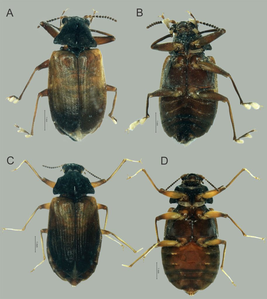
Figura 1. Vista dorsal y ventral del macho y hembra de Psephenops oaxacanus. A) Hábito dorsal; B) hábito ventral; C) hábito dorsal; D) hábito ventral.
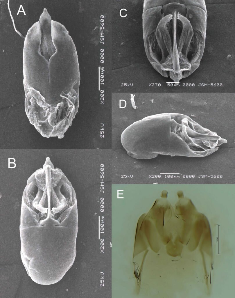
Figura 2. Vista del genital masculino y femenino de Psephenops oaxacanus. A) Vista dorsal; B) vista ventral; C) vista frontal; D) vista ventrolateral; E) vista ventral del genital femenino mostrando los estilos, gonocoxitos y laterotergitos.
Resumen taxonómico
Material tipo. Holotipo macho. México: localidad tipo, estado de Oaxaca, Municipio Santiago Comaltepec, San Martín Soyolapam, río Soyolapam, 136 m snm (17°41’58” N, -96°16’59” O), 5.II.2016. Cols. J.A. Gómez et R. Novelo [escrito a máquina, etiqueta blanca], “Holotype ♂/ Psephenops oaxacanus nov. sp. / Arce-Pérez, Gómez-Anaya & Novelo-Gutiérrez 2025” [escrito a máquina, etiqueta roja], Paratipos: 5 ♂, 6 ♀ mismos datos del holotipo [escrito a máquina, etiqueta amarilla] (IEXA).
Etimología. Esta especie recibe el nombre oaxacanus por ser la primera especie de la subfamilia Psepheninae y del género Psephenops para el estado de Oaxaca, México.
El holotipo y paratipos se encuentran depositados en la Colección Entomológica del Instituto de Ecología, A.C., Xalapa, México (IEXA), con el número de catálogo IEXA-2025-IM20.
Comentarios taxonómicos
Se considera más estrechamente relacionada con P. mexicanus por presentar ambas el mismo tipo de antenas cortas y moniliformes, parámeros en vista dorsal subtriangulares, separados por un profundo surco y fusionados en su base (figs. 2a, 6c), además por el tamaño corporal de 3 a 3.5 mm. Con base en la literatura disponible, la nueva especie puede distinguirse de las de México, América Central y las Antillas por las características anotadas en la tabla 1.
Hábitat. El río Soyolapam se localiza en la localidad del mismo nombre en la sierra de Juárez, Oaxaca, en la subcuenca del río Valle Nacional (fig. 4), el tipo de vegetación es selva alta perennifolia a una altitud de 136 m snm. El río presenta en su cauce cantos y rocas emergentes cubiertas parcialmente por algas y vegetación abundante en sus márgenes, los cuales en algunas partes son playones arenosos (fig. 3).
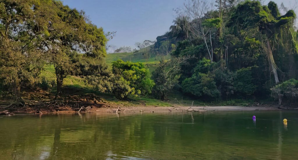
Figura 3. Localidad tipo de Psephenops oaxacanus en el río Sayolapam (San Martín), Santiago Comaltepec, Oaxaca, México (febrero de 2016).
Hasta el momento, esta especie solo está presente en Oaxaca, al sur de México, en el río Soyolapan, a 136 m snm (fig. 4). La localidad tipo se encuentra en la parte norte del estado, en la provincia sierra Madre del Sur, en la subprovincia de los Altos de Oaxaca. Esta especie se recolectó sintópicamente con ejemplares de los géneros Cylloepus y Macrelmis de la familia Elmidae.
Lista actualizada de las especies de Psephenops Grouvelle en México.
Psephenops lupita (Arce-Pérez)
Psephenops lupita (Arce-Pérez, 2002: 964)
Registros publicados. México: Veracruz: Municipio Coatepec, Poblado Coatepec, río Huehueyapan (Sección La Marina), 19º26’55” N, 96º58’52” O, 1, 200 m, bosque mesófilo de montaña (fig. 4); municipio Xico, Poblado Xico Viejo, río Malseseca, 19º26’44.89” N, 97º03’22.22” O, 1,800 m, bosque mesófilo de montaña (fig. 4).
Psephenops mexicanus (Arce-Pérez y Novelo-Gutiérrez)
Psephenops mexicanus (Arce-Pérez y Novelo-Gutiérrez, 2000: 196)
Registros publicados. México: Veracruz: Municipio Coatepec, Poblado Coatepec, río Huehueyapan (Sección La Marina), 19º26’55” N, 96º58’52” O, 1,200 m, bosque mesófilo de montaña (fig. 4); municipio Xico, Poblado Xico Viejo, río Malseseca, 19º26’44.89” N, 97º03’22.22” O, 1,800 m, bosque mesófilo de montaña (fig. 4).
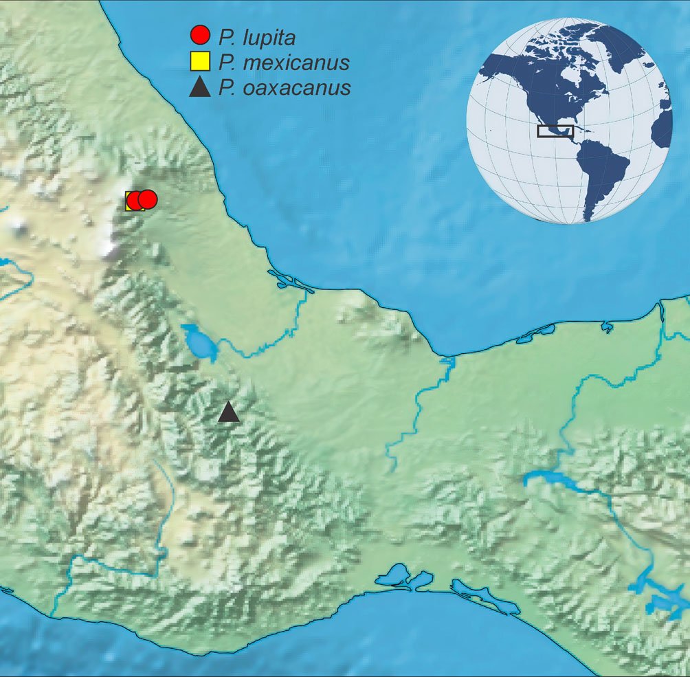
Figura 4. Distribución de las especies de Psephenops en México.
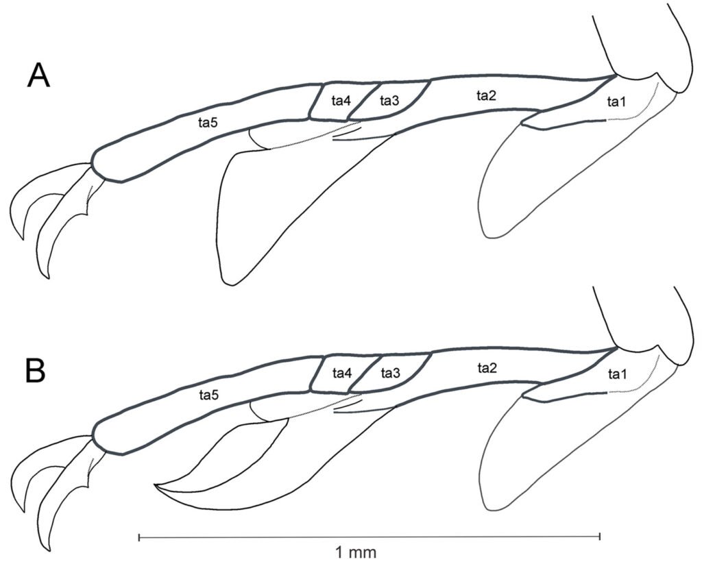
Figura 5. Vista lateral de las patas mostrando lóbulos tarsales en Psephenops spp. A) Cortos; B) largos, ta = tarsómeros.
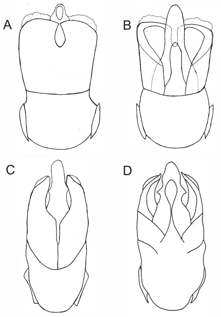
Figura. 6 A-D. Vista del genital masculino de P. lupita y P. mexicanus. A) Dorsal; B) ventral; C) dorsal; D) ventral. Figuras A, B tomadas de Arce-Pérez (2002); C, D tomadas de Arce-Pérez y Novelo-Gutierrez (2000).
Clave para la identificación de las especies mexicanas de Psephenops Grouvelle (modificada de Arce-Pérez y Novelo-Gutiérrez, 2013, 2017)
1 Antenas filiformes, largas, tocando base de pronoto; parámeros en vista dorsal anchos, subcuadrados y fusionados en base en ligera hendidura en forma de gota (fig. 6a), en vista ventral lóbulo medio y esclerito interno digitiformes (fig. 6b); lóbulos tarsales cortos, sin alcanzar más de 0.5 basales del tarsómero 5 (fig. 5a); longitud total 3.75 – 3.85 mm P. lupita
1’ Antenas cortas, moniliformes, no tocan base del pronoto; parámeros en vista dorsal subtriangulares, separados por hendidura que va de ligera a profunda (figs. 2a, 6c); en vista ventral lóbulo medio y esclerito interno no digitiformes; lóbulos tarsales cortos o largos (figs. 5a, b) 2
2 (1’) Lóbulos tarsales largos, cubriendo 0.8 basales del tarsómero 5 (fig. 5b); parámeros en vista dorsal con profunda hendidura longitudinal media (fig. 6c); en vista ventral lóbulo medio subtriangular, con dientecillo a cada lado; esclerito interno del lóbulo medio lanceolado (fig. 6d); longitud 3.15 – 3.55 mm P. mexicanus
2’ Lóbulos tarsales cortos, sin alcanzar más de 0.5 basales del tarsómero 5 (fig. 5a); parámeros en vista dorsal separados por profunda hendidura ancha en forma de lanza invertida y continuada por ligera hendidura que no los separa (fig. 2a); en vista ventral lóbulo medio digitiforme sin dientecillos laterales, terminando en punta ancha, con esclerito interno esbelto, claviforme hacia el ápice, en vista lateral agudo (figs. 2b-d); longitud 3.0 – 3.5 mm P. oaxacanus sp. nov.
Agradecimientos
A Emmanuel Arriaga Varela (INECOL) y a un revisor anónimo por sus atinadas correcciones y sugerencias que mejoraron el manuscrito final.
Referencias
Arce-Pérez, R. (2002). A new species of Psephenops Grouvelle (Coleoptera: Psephenidae) from Mexico. Proceedings of the Entomological Society of Washington, 104, 964–967.
Arce-Pérez, R. y Novelo-Gutiérrez, R. (2000). First record of the genus Psephenops (Coleoptera: Psephenidae) from Mexico, with a description of a new species. Entomological News, 111, 196–200.
Arce-Pérez, R. y Novelo-Gutiérrez, R. (2013). Two new species of Psephenops Grouvelle from Belize (Coleoptera: Byrrhoidea: Psephenidae), with a key to the known species from Mexico and Central America. Zootaxa, 3670, 63–70. http://dx.doi.org/10.11646/zootaxa.3670.1.5
Arce-Pérez, R. y Novelo-Gutiérrez, R. (2017). Two new species of Psephenops Grouvelle (Coleoptera: Byrrhoidea: Psephenidae) from Panama. Zootaxa, 4323, 109–118. https://doi.org/10.11646/zootaxa.4323.1.8
Arce-Pérez, R., Novelo-Gutiérrez, R. y Cornejo, A. (2015). Psephenops panamaensis sp. nov. (Coleoptera: Byrrhoidea: Psephenidae) from Panamá. Zootaxa, 4052, 233–236. https://doi.org/10.11646/zootaxa.4052.2.8
Bameul, F. (2001). Un nouveau Psephenops Grouvelle de la Guadeloupe, avec la description de sa larve (Coleoptera, Psephenidae). Nouvelle Revue d’Entomologie, 18, 161–172.
Barr, C. B. y Shepard, W. D. (2024). A taxonomic review of the genus Psephenops Grouvelle of the Lesser Antilles with description of new species Psephenops trini, and reassignment of Peruvian species Psephenus robacki Spangler (Coleoptera: Psephenidae: Psepheninae). Insecta Mundi, 1045, 1–22. https://doi.org/10.5281/zenodo.11450152
Deléve, J. (1967). Contribution á l’ étude des Dryopoidea (Coleoptera). XIX. Notes diverses et descriptions d’ spéces nouvelles. Bulletin et Annales de la Société Entomologique de Belgique, 103, 414–446.

COI based phylogeny and morphological characterizationof a Brazilian population of Lambornella trichoglossa(Ciliophora: Tetrahymenidae)
Filogenia basada en COI y caracterización morfológica de una población brasileña de Lambornella trichoglossa (Ciliophora: Tetrahymenidae)
Vítor Ribeiro-Halfeld *
Universidade Federal de Juiz de Fora, Laboratório de Protozoologia, Rua José Lourenço Kelmer, s/n, São Pedro, Juiz de Fora, 36033-900 Minas Gerais, Brazil
*Corresponding author: ribeirohalfeldv@gmail.com (V. Ribeiro-Halfeld)
Received: 28 July 2025; accepted: 22 October 2025
Abstract
In this work, the morphological characterization and molecular phylogeny (SSU rDNA and COI) of Lambornella trichoglossa Foissner, 2003, found in phytotelmata environments in southeastern Brazil is presented. The morphological study performed with silver impregnation techniques demonstrated parameters similar to those recorded in the type population, and additional new information was also obtained, including the conjugation process and the occurrence of specimens with an increased number of caudal cilia. The phylogenetic reconstructions based on both markers suggest the inclusion of L. trichoglossa in the genus Tetrahymena Furgason, 1940. The COI sequence obtained in this work is the first mitochondrial sequence of the genus Lambornella deposited in GenBank and published in a scientific article.
Keywords: Tetrahymena; Phytotelmata; Molecular phylogeny
Resumen
En este trabajo se realizó la caracterización morfométrica y la filogenia molecular (SSU rDNA y COI) de Lambornella trichoglossa Foissner, 2003, encontrada en ambientes de fitotelmata en el sureste de Brasil. El estudio morfológico realizado con técnicas de impregnación de plata demostró parámetros similares a los registrados en la población tipo y también se obtuvo nueva información adicional, incluyendo el proceso de conjugación y la presencia de especímenes con un mayor número de cilios caudales. Las reconstrucciones filogenéticas basadas en ambos marcadores sugieren la inclusión de L. trichoglossa en el género Tetrahymena Furgason, 1940. La secuencia COI obtenida en este trabajo es la primera de tipo mitocondrial del género Lambornella depositada en GenBank y publicada en un artículo científico.
Palabras clave: Tetrahymena; Fitotelmas; Filogenia molecular
Introduction
The genus Lambornella has its systematic history marked by alterations. The type species, Lambornella stegomyiae Keilin, 1921, is a mosquito (Diptera, Culicidae) parasite. It was reclassified in the genus Tetrahymena Furgason, 1940 by Corliss (1960). However, the description of Lambornella clarki Corliss, 1976, another parasitic species, revalidated the genus, indicating the formation of cuticular cysts and the number of post-oral kineties as diagnostic features. Nevertheless, Strüder-Kypke et al. (2001) suggested the non-validity of the genus Lambornella once again, due to its position within the Tetrahymena clade, based on phylogenetic analyses inferred from small subunit ribosomal DNA (SSU). Results presented by Bourland and Stüder-Kypke (2010), and Dunthorn et al. (2012), also based on SSU sequences, demonstrated a similar grouping.
Lambornella trichoglossa Foissner, 2003 is the only free-living species of the genus. It occurs endemically in phytotelmata environments (Foissner, 2003). Despite the recurrent records in the Neotropical region (Buosi et al., 2014, 2015; Durán-Ramírez et al., 2015; Foissner, 2003; Foissner et al., 2003), no studies have investigated Lambornella’s phylogenetic position based on mitochondrial markers. According to Chantangsi and Lynn (2008), the mitochondrial gene cytochrome c oxidase-subunit I (COI) is effective in elucidating recent phylogenetic events in the genus Tetrahymena. In this context, the present work aimed to investigate the molecular phylogeny of L. trichoglossa based on the mitochondrial marker COI. Morphological analysis of the specimens was also performed in order to confirm specific identification and investigate possible morphological variation.
Materials and methods
One hundred milliliters of phytotelmata content were collected from 12 bromeliads belonging to Portea petropolitana at the Botanical Garden of the Federal University of Juiz de Fora (21°43’74” S, 43°22’06” W), in September, 2019. On the same day of collections, the samples were analyzed under a stereoscopic microscope with transmitted light. Active ciliates were picked with glass micropipettes and processed, according to Foissner (2014), to perform silver carbonate and dry silver nitrate impregnation techniques. From the collection day, over a period of 7 days, 20 specimens of L. trichoglossa were screened from the samples and measured in vivo to check for possible alterations in body length. Obtained data were analyzed using the Shapiro-Wilk normality test, and the means recorded on the first and seventh days were compared using the Student’s t-test. All statistical analyses related to the morphological data were conducted using PAST software, version 4.03 (Hammer et al., 2001).
Thirty specimens of L. trichoglossa were picked from the samples and fixed in absolute ethanol for molecular analysis. Total DNA extraction was performed using the Blood and Tissue kit (Qiagen®), following the manufacturer’s guidelines. Primers F388dT and R1184dT (Strüder-Kypke & Lynn, 2010) were used to amplify the COI gene in 25-microliter reactions. The SSU marker was also sequenced for comparison with the type population. Therefore, primers 18S F9Euk and 18S R1513 (Schrallhammer et al., 2013) were used.
PCR products were visualized in a 1% agarose gel and purified using the QIAquick PCR Purification Kit (Qiagen®), following the manufacturer’s guidelines. Subsequently, the material was sent for sequencing according to the Sanger method in 7 µl reactions, using the M13 forward and M13 reverse primers (Messing, 1983) for COI, and 18S R536, 18S F783, 18S F919, and 18S R1052 for SSU (Modeo et al., 2006). Sequencing reactions were performed on an ABI PRISM® 3100 sequencer (Applied Biosystems).
Obtained sequences were added to the respective datasets, jointly with COI and SSU sequences of approximately 20 species of the genus Tetrahymena, as well as outgroups obtained from GenBank accessed in May 2025. Sequences were aligned using MAFFT software, version 7 (Katoh et al., 2017). The resulting alignment was edited in the GBlocks platform, version 0.91b (Talavera & Catresana, 2007). The determination of the best nucleotide substitution model (GTR + G + I to COI, and TN93 + G to SSU) was performed with the aid of MegaX software (Kumar et al., 2018), using the maximum likelihood method, considering all sites. The maximum likelihood phylogenetic analysis was inferred using RAxML software, version 8 (Stamatakis, 2014), at its default settings, with 500 bootstrap replicates for COI, and 1,200 for SSU. The evolutionary distances of COI and SSU sequences were computed in Mega X, using the Kimura 2-parameter method (Kimura, 1980). A third dataset with 74 COI sequences of Tetrahymena species was prepared, in addition to outgroups, with the aim of performing the pairwise distance calculations with a greater number of species (Supplementary material). For this analysis, the Maximum Composite Likelihood model (Tamura et al., 2004) was used, with the aid of MegaX (Kumar et al., 2018).
Results
Table 1 presents the morphological data obtained. Morphological characterization of the L. trichoglossa population analyzed in this study resembles the type population described by Foissner (2003), presenting slightly higher values for body size and the number of somatic kineties. However, postoral kineties appear in lower numbers. Another important morphological characteristic distinct from the type population detected in the present study was the occurrence of specimens with a greater number of caudal cilia (Fig. 1h). These organisms have a complex of caudal cilia, as shown in Figure 1h and Supplementary material. However, they were not included in the morphological statistical analysis due to the unsatisfactory results of the impregnation techniques in their oral and some somatic structures. Opportunely, conjugating forms of L. trichoglossa were recorded, which is unprecedented for the species (Fig. 1a). The temporal analyses on body length performed demonstrated a significant decrease in the average size of the organisms over 7 days (Fig. 2, Table 2).
The obtained SSU sequence was deposited in GenBank with accession number MN567691. It matches 99.97% of the type population’s sequence (AJ810078) (Table 3). The phylogenetic reconstruction inferred by the maximum likelihood method revealed that the new sequence is grouped with L. trichoglossa (AJ810078), T. corlissi (U17356), and T. berger (AF364039) (Fig. 3).
Lambornella trichoglossa’s COI sequence was deposited in GenBank with accession number MN477017. It has 774 nucleotides, with the following percentage of bases: A = 33%, C = 12%, G = 13.4%, and T = 41.6%. Phylogenetic reconstruction using the maximum likelihood method demonstrated L. trichoglossa clustering in a clade with the same topology revealed by the SSU phylogeny; it also grouped with T. corlissi (EF070279) and T. bergeri (EF070270) with a support value of 86%, besides T. scolopax (KJ028669) (Fig. 4). The average paired difference of the 74 Tetraymena sequences used in the phylogenetic analyses was 12.99%. The L. trichoglossa sequence differs by 13.04% from the T. corlissi sequence (Table 4). Although the value is slightly above the average for the Tetrahymena species analyzed, this percentage is lower than the difference observed between T. corlissi and T. caudata (14.29%), T. paravorax (14%), and T. glochidiophila (16.39%), for example.
Table 1
Morphological data on silver carbonate-impregnated specimens of Lambornella trichoglossa.
| x | M | SD | SE | CV | Min | Max | n | |
| Body, lenght | 269.75 | 269.43 | 26.72 | 4.88 | 9.906 | 226.65 | 327.91 | 30 |
| Body, width in ventral view | 73.105 | 73.295 | 16.05 | 2.93 | 21.96 | 47.44 | 107.77 | 30 |
| Body lenght: Lateral width, ratio | 3.82 | 3.906 | 0.81 | 0.14 | 21.19 | 2.606 | 5.36 | 30 |
| Anterior body end to membranelle 1, distance | 47.91 | 48.73 | 7.407 | 1.35 | 15.46 | 34.14 | 63.87 | 30 |
| Oral opening, width | 32.45 | 31.42 | 5.11 | 0.93 | 15.77 | 21.28 | 44.12 | 30 |
| Anterior body end to macronucleus, distance | 94.55 | 92.88 | 13.86 | 2.53 | 14.66 | 74.16 | 126.35 | 30 |
| Macronucleus, length | 49.72 | 43.96 | 11.48 | 2.09 | 23.08 | 36.92 | 77.75 | 30 |
| Macronucleus, width | 51.27 | 48.71 | 9.42 | 1.72 | 18.38 | 33.74 | 66.86 | 30 |
| Macronucleus, number | 1 | 1 | 0 | 0 | 0 | 1 | 1 | 30 |
| Micronucleus, width | 5.67 | 5.5 | 1.15 | 0.21 | 20.408 | 4 | 9.56 | 27 |
| Micronucleus, number | 1.03 | 1 | 0.19 | 0.035 | 18.68 | 1 | 2 | 27 |
| Somatic kineties, total number | 52.33 | 52.5 | 3.79 | 0.69 | 7.24 | 45 | 62 | 30 |
| Somatic kineties, postoral number | 6.1 | 6 | 0.84 | 0.15 | 13.85 | 5 | 8 | 30 |
| Caudal cilia, number | 1 | 1 | 0 | 0 | 0 | 1 | 1 | 30 |
Measurements in μm. x, arithmetic mean. M, median. SD, standard deviation. SE, standard error of arithmetic mean. CV, coefficient of variation (%). Min, minimum. Max, maximum. n, number of individuals investigated.
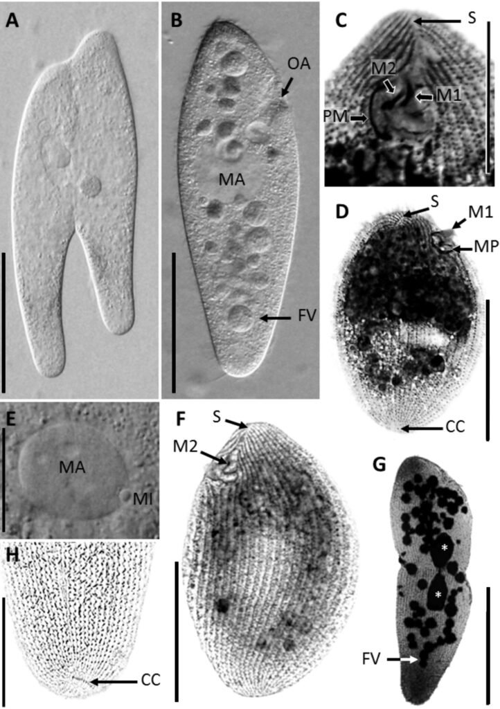
Figure 1. Morfological characterization of Lambornella trichoglossa. A, B, E. In vivo. C, D, F. Dry silver impregnation. G, H. Silver Carbonate impregnation. A, First recorded conjugating specimens; B, lateral view; C, oral apparatus; D, specimen with normal number of caudal cilium (dorsal view); E, nuclear apparatus; F, ventral view, showing oral apparatus and postoral kineties, below; G, specimen recorded during divisional morphogenesis, with multiple food vacuoles scattered throughout the body; H, detail of caudal cilia complex recorded in larger specimens. OA (oral apparatus), FV (food vacuoles), S (preoral suture), PM (paroral membrane), M1 and M2 (adoral membranelles), MA (macronucleus), MI (micronucleus), CC (caudal cilia). Asterisks indicate macronucleus during divisional morphogenesis process. Scale bars in A, B, D, F, G = 100 μm. In C, E H = 50μm.
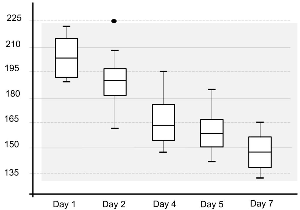
Figure 2. Body length reduction of L. trichoglossa over a 7-day period.
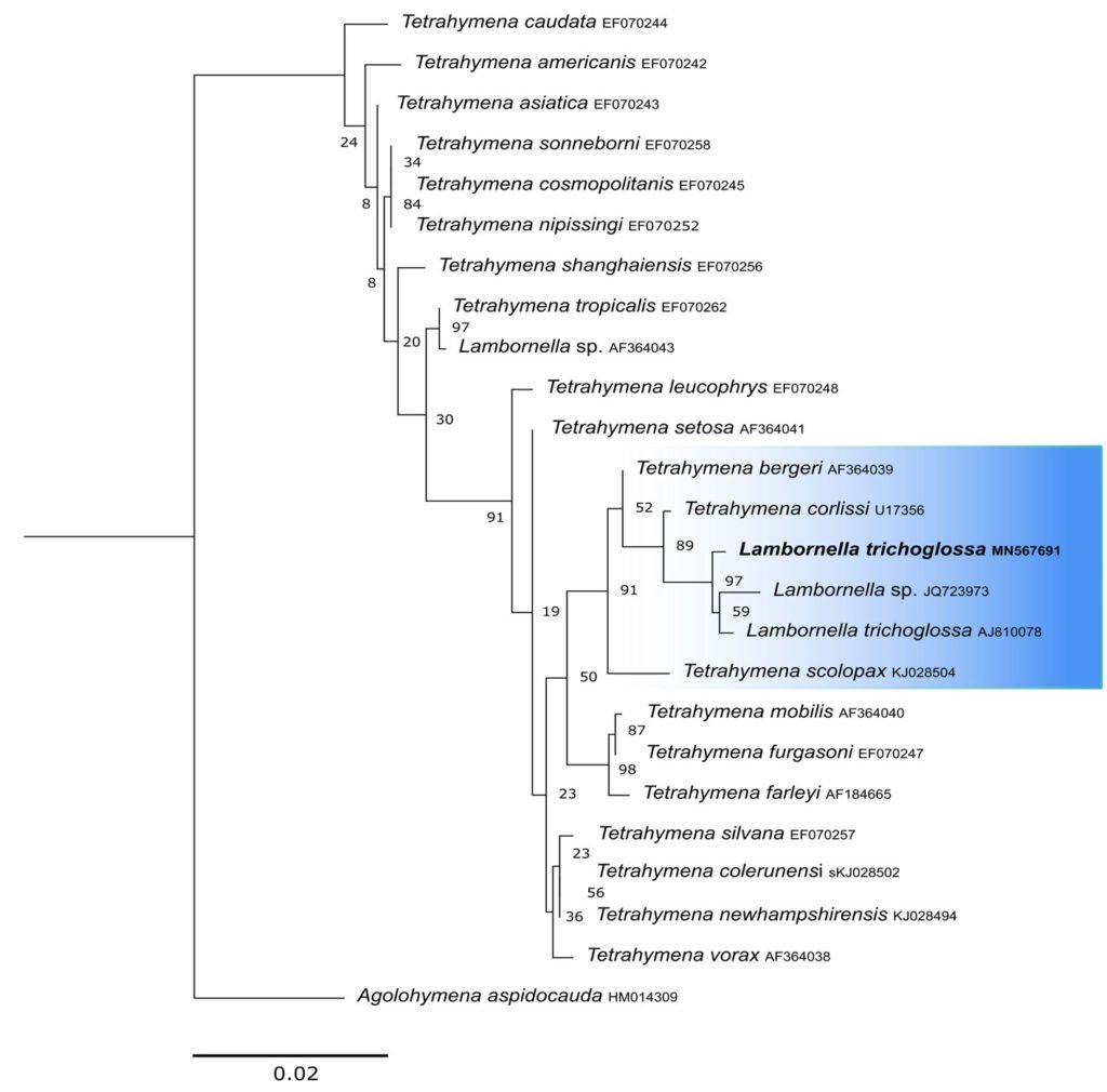
Figure 3. Maximum likelihood (ML) tree inferred from small subunit ribosomal DNA (SSU rDNA). Bold: sequence obtained in the present work. Numbers at nodes represent the bootstrap values of ML out of 1,200 replicates.
Table 2
Statistical data on the difference in body length of L. trichoglossa 7 days after collection.
| Number of measured specimens | |
| 1st day | 20 |
| 7th day | 20 |
| Body length mean (μm) | |
| 1st day | 205.66 |
| 7th day | 148.255 |
| Maximum length (μm) | |
| 1st day | 222.79 |
| 7th day | 164.84 |
| Minimum length (μm) | |
| 1st day | 190.18 |
| 7th day | 132.43 |
| Standart deviation | |
| 1st day | 10.97027077 |
| 7th day | 10.06698748 |
| Variance | |
| 1st day | 120.3468408 |
| 7th day | 101.3442368 |
| Shapiro-Wilk test (α = 0.05) | |
| 1st day | W: 0.9273 |
| p-value: 0.1371 | |
| 7th day | W: 0.9556 |
| p-value: 0.4607 | |
| Student’s t-test | |
| t: 17.241 | |
| p: 1.47.10-19 | |
| Critical t-value (p = 0.05): 2.0244 |
Discussion
The similarity of the morphological parameters between the specimens analyzed in the present study and the data presented in the description of L. trichoglossa ensures the correct taxonomic identification of the organisms. It should be noted that the characterization performed by Foissner (2003) occurred a few days after collection, whereas in the present work, the morphological study techniques were performed a few hours after collection. The temporal analyses on body length performed in the present work demonstrated a decrease in the average size of the organisms over time (Fig. 2), which would justify the slightly higher average values compared to the type population.
Regarding the occurrence of specimens with a greater number of caudal cilia, polymorphic life cycles are a common characteristic of the genus Tetrahymena. Lynn and Doerder (2012) mentioned the occurrence of changes in size, body shape, organization, morphology, and cilia of the oral apparatus of Tetrahymena species, due to environmental changes. The aforementioned authors highlighted the great genotypic and phenotypic plasticity found in the clade.
Phylogenetic reconstructions performed with both markers demonstrate the internal position of L. trichoglossa in the genus Tetrahymena, corroborating analyses based on the SSU marker presented by Strüder-Kypke et al. (2001), Bourland and Strüder-Kypke (2010), and Dunthorn et al. (2012). Several authors demonstrated the division of the genus Tetrahymena into 2 strongly molecularly supported clades, Australis and Borealis (Chantangsi, 2007; Chantangsi & Lynn, 2008; Lynn et al., 2018; Nanney, 1998; Strüder-Kypke et al., 2001). This division was observed in the inferred reconstructions by the SSU marker, performed in the present study, demonstrating the inclusion of L. trichoglossa into the Borealis clade. Doerder (2018) states that this clade has greater molecular diversity and more species than the Australis clade, thus being an important source of diversity for the genus. Lambornella trichoglossa, included in this clade, is the greatest example of phenotypic diversification, given its morphological and ontogenetic particularities demonstrated by Foissner (2003).
The phylogenetic analyses inferred by the COI gene demonstrated the inclusion of L. trichoglossa in a clade called coxset A4 by Chantangsi and Lynn (2008). The species T. corlissi and T. bergeri, members of this clade, share the parasitic lifestyle and have particular morphological characteristics (Hoffman et al., 1975; Imai et al., 2000; Strüder-Kypke et al., 2001). Foissner (2003) performed infection tests with L. trichoglossa and different mosquito species, noting that the ciliate does not develop a parasitic association. However, congeners L. stegomyiae and L. clarki are parasites of culicid dipterans, demonstrating that this way of life is predominant in coxiset A4, corroborating Chantangsi and Lynn (2008). Probably, parasitism also represents the ancestral condition of this clade, since Strüder-Kypke et al. (2001) demonstrated that histophagy is a recurrent phenomenon in the evolution of Tetrahymena.
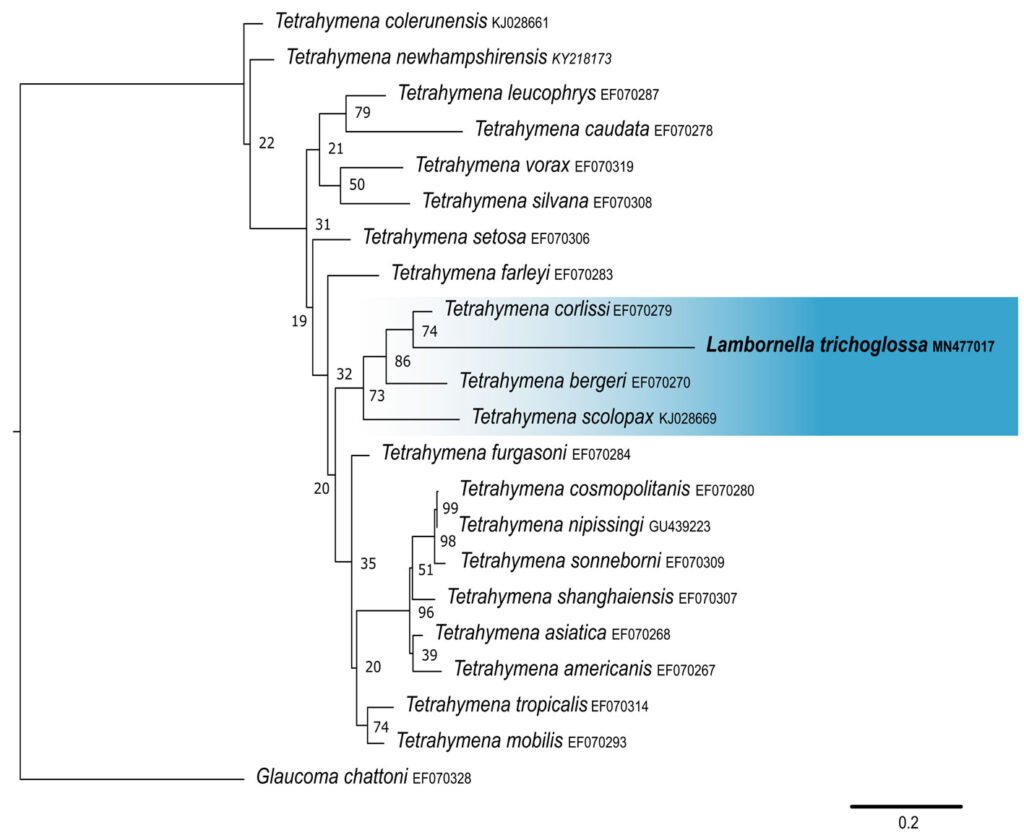
Figure 4. Maximum likelihood (ML) tree inferred from cytochrome oxidase subunit I (COI). Bold: sequence obtained in the present work. Numbers at nodes represent the bootstrap values of ML out of 500 replicates.
Table 3
Pairwise distance between SSU sequences of Lambornella trichoglossa and Tetrahymena spp.
| MN567691 | L. trichoglossa | ||||||||
| AJ810078 | L. trichoglossa* | 0.0029 | |||||||
| JQ723973 | Lambornella sp.** | 0.0053 | 0.0047 | ||||||
| U17356 | T. corlissi | 0.0059 | 0.0063 | 0.0077 | |||||
| AF364039 | T. bergeri | 0.0071 | 0.0092 | 0.0089 | 0.0046 | ||||
| EF070247 | T. furgasoni | 0.0130 | 0.0149 | 0.0149 | 0.0099 | 0.0092 | |||
| AF364040 | T. mobilis | 0.0130 | 0.0151 | 0.0149 | 0.0104 | 0.0092 | 0.0006 | ||
| KJ028502 | T. colerunensis | 0.0132 | 0.0139 | 0.0139 | 0.0087 | 0.0080 | 0.0051 | 0.0058 | |
| KJ028504 | T. scolopax | 0.0135 | 0.0156 | 0.0156 | 0.0094 | 0.0067 | 0.0135 | 0.0142 | 0.0125 |
Bold font: sequence obtained in the present study. * Sequence obtained from the type population (Dunthorn et al., 2012). ** Sequences obtained from samples collected in Jamaica (Dunthorn et al., 2012).
Table 4
Pairwise distance between COI sequences of Lambornella trichoglossa and Tetrahymena spp.
| MN477017 | L. trichoglossa | |||||||||
| EF070279 | T. corlissi | 0.1294 | ||||||||
| EF070270 | T. bergeri | 0.1450 | 0.0921 | |||||||
| EF070291 | T. malaccensis | 0.1536 | 0.1187 | 0.1320 | ||||||
| EF070268 | T. asiatica | 0.1557 | 0.1026 | 0.1113 | 0.1062 | |||||
| KY218158 | T. alphathermophila | 0.1713 | 0.1152 | 0.1403 | 0.1175 | 0.1281 | ||||
| EF070296 | T. paravorax | 0.1961 | 0.1400 | 0.1491 | 0.1413 | 0.1185 | 0.1407 | |||
| KJ028669 | T. scolopax | 0.1982 | 0.1364 | 0.1376 | 0.1461 | 0.1184 | 0.1534 | 0.1491 | ||
| EF070278 | T. caudata | 0.1857 | 0.1429 | 0.1492 | 0.1622 | 0.1331 | 0.1553 | 0.1735 | 0.1615 | |
| MF693881 | T. glochidiophila | 0.2187 | 0.1639 | 0.1867 | 0.1626 | 0.1631 | 0.1703 | 0.1500 | 0.1926 | 0.2051 |
Bold font: sequence obtained in the present study.
Traditionally recognized Tetrahymena species, described based on morphological or biochemical characteristics, and molecularly supported, may have high evolutionary difference values when comparing COI sequences. For example, T. caudata differs by over 15% from T. corlissi, T. termophila, and T. glochidiophila. Some species described by Doerder (2018) based mainly on molecular diversity differ by values close to 20%. Therefore, the 12.94% distance observed between the COI sequence of L. trichoglossa and T. corlissi does not represent a discrepancy concerning the molecular variability observed in Tetrahymena.
According to Chantangsi and Lynn (2008), the mitochondrial COI gene is effective in elucidating Tetrahymena’s recent phylogeny, while the SSU marker is more suited to assessing the deep phylogeny of the genus. The maintenance of topology in the reconstructions performed with both markers demonstrates that L. trichoglossa, T. corlissi, and T. bergeri share a long evolutionary history, and the differentiation of the species belonging to the genus Lambornella could be recent within the phylogeny of Tetrahymena. The phylogenetic position of L. trichoglossa also demonstrated by the COI gene, reinforces the proposals for synonymization of the genera Lambornella and Tetrahymena. Although Lambornella’s description precedes that of Tetrahymena, the principle of stability is appropriate to maintain the name of the latter taxon. In any case, it is necessary to establish an extended diagnosis for Tetrahymena, so that the species involved in new combinations are covered.
Finally, the molecular analysis of L. trichoglossa based on the COI marker supports the proposal for synonymization of the genera Lambornella and Tetrahymena. This systematic readjustment also points to the great molecular, morphological, evolutionary and ecological complexity of the genus Tetrahymena, which represents one of the greatest examples of evolutionary adaptation among eukaryotic organisms.
References
Bourland, W. A., & Strüder-Kypke, M. (2010). Agolohymena aspidocauda nov. gen., nov.spec., a histophagous freshwater tetrahymenid ciliate in the family Deltopylidae (Ciliophora, Hymenostomatia), from Idaho (northwest U.S.A.): morphology, ontogenesis and molecular phylogeny. European Journal of Protistology, 46, 221–242. https://doi.org/10.1016/j.ejop.2010.04.003
Buosi, P. R. B., Utz, L. R. P., Meira, B. R., Silva, B. T. S., Lansac-Tôha, F. M., Lansac-Tôha, F. A. et al. (2014). Rainfall influence on species composition of the ciliate community inhabiting bromeliad phytotelmata. Zoological Studies, 53, 32–44. https://doi.org/10.1186/s40555-014-0032-4
Buosi, P. R. B., Cabral, A. F., Utz, L. R. P., Vieira, L. C. G., & Velho, L. F. M. (2015). Effects of seasonality and dispersal on the ciliate community inhabiting bromeliad phytotelmata in riparian vegetation of a large tropical river. Journal of Eukaryotic Microbiology, 62, 737–749. https://doi.org/10.1111/jeu.12232
Chantangsi, C., & Lynn, D. H. (2008). Phylogenetic relationships within the genus Tetrahymena inferred from the cytochrome c oxidase subunit 1 and the small subunit ribosomal RNA genes. Molecular Phylogenetics and Evolution, 49, 979–87. https://doi.org/10.1016/j.ympev.2008.09.017
Chantangsi, C., Lynn, D. H., Brandl, M. T., Cole, J. C., Hetrick, N., & Ikonomi, P. (2007). Barcoding ciliates: a comprehensive study of 75 isolates of the genus Tetrahymena. International Journal of Systematic and Evolutionary Microbiology, 57, 2412–2423. https://doi.org/10.1099/ijs.0.64865-0
Corliss, J. O., & Coats, D. W. (1976). A new cuticular cyst-producing tetrahymenid ciliate, Lambornella clarki n. sp., and the current status of ciliatosis in culicine mosquitoes. Transactions of the American Microscopical Society, 95, 725–739. https://doi.org/10.2307/3225400
Corliss, J. O. (1960). Tetrahymena chironomi sp. nov., a ciliate from midge larvae, and the current status of facultative parasitism in the genus Tetrahymena. Parasitology, 50, 111–153. https://doi.org/10.1017/S0031182000025245
Doerder, F. P. (2018). Barcodes reveal 48 new species of Tetrahymena, Dexiostoma, and Glaucoma: phylogeny, ecology, and biogeography of new and established species. Journal of Eukaryotic Microbiology, 66, 182–208. https://doi.org/10.1111/jeu.12642
Dunthorn, M., Stoeck, T., Wolf, K., Breiner, H., & Foissner, W. (2012). Diversity and endemism of ciliates inhabiting Neotropical phytotelmata. Systematics and Biodiversity, 10, 195–205. https://doi.org/10.1080/14772000.2012.685195
Durán-Ramírez, C., García-Franco, J. G., Foissner, W., & Mayén-Estrada, R. (2015). Free-living ciliates from epiphytic tank bromeliads in Mexico. European Journal of Protistology, 51, 15–33. https://doi.org/10.1016/j.ejop.2014.09.002
Foissner, W. (2003). Morphology and ontogenesis of Lambornella trichoglossa nov. spec., a new tetrahymenid ciliate (Protozoa,Ciliophora) from Brazilian tank bromeliads (Bromeliaceae). European Journal of Protistology, 39, 63–82. https://doi.org/10.1078/0932-4739-00887
Foissner, W. (2014). An update of basic light and scanning electron microscopic methods for taxonomic studies of ciliated protozoa. International Journal of Systematic and Evolutionary Microbiology, 64, 271–292. https://doi.org/10.1099/ijs.0.057893-0
Foissner, W., Strüder-Kypke, M., van der Staay, G. W. M., van der Staay, S. M., & Hackstein, J. H. P. (2003). Endemic ciliates (Protozoa,Ciliophora) from tank bromeliads (Bromeliaceae): a combined morphological, molecular, and ecological study. European Journal of Protistology, 39, 365–372. https://doi.org/0.1078/0932-4739-00005
Hammer, Ø., Harper, D. A. T., & Ryan, P. D. (2001). PAST: Paleontological Statistics Software Package for Education and Data Analysis. Palaeontologia Electronica, 4, 1–9.
Hoffman, G. L., Lando, M., Camper, J. E., Coats, D. W., Stookey, J. L., & Burek, J. D. (1975). A disease of freshwater fishes caused by Tetrahymena corlissi Thompson, 1955, and a key for identification of holotrich ciliates of freshwater fishes. The Journal of Parasitolgy, 61, 217–223. https://doi.org/10.1111/j.1365-2761.2009.01062.x
Imai, S., Tsurimaki, S., Goto, E., Wakita, K., & Hatai, K. (2000). Tetrahymena infection in Guppy, Poecilia reticulata. Fish Pathology, 35, 67–72. https://doi.org/10.3147/jsfp.35.67
Katoh, K., Rozewicki, J., & Yamada, K. D. (2017). MAFFT online service: multiple sequence alignment, interactive sequence choice and visualization. Briefings in Bioinformatics, 20, 1160–1166. https://doi.org/10.1093/bib/bbx108
Keilin, D. (1921). On a new ciliate: Lambornella stegomyiae n. g., n. sp., parasitic in the body-cavity of the larvae of Stegomyia scutellaris Walker (Diptera, Nematocera, Culicidae). Parasitology, 13, 216–224. https://doi.org/10.1017/s0031182000012488
Kimura, M. (1980). A simple method for estimating evolutionary rate of base substitutions through comparative studies
of nucleotide sequences. Journal of Molecular Evolution, 16, 111–120. https://doi.org/10.1007/BF01731581
Kumar, S., Stecher, G., Li, M., Knyaz, C., & Tamura, K. (2018). MEGA X: Molecular Evolutionary Genetics Analysis across Computing Platforms. Molecular Biology and Evolution, 35, 1547–1549. https://doi.org/10.1093/molbev/msy096
Lynn, D. H., & Doerder, F. P. (2012). The life and times of Tetrahymena. In Collins, K. Methods in cell biology. Elsevier, 109, 9–27. https://doi.org/10.1016/B978-0-12-385
967-9.00002-5
Lynn, D. H., Doerder, F. P., Gillis, P. L., & Prosser, R. S. (2018). Tetrahymena glochidiophila n. sp., a new species of Tetrahymena (Ciliophora) that causes mortality to glochidia larvae of freshwater mussels (Bivalvia). Diseases of Aquatic Organisms, 127, 125–136. https://doi.org/10.3354/dao03188
Lynn, D. H. (2008). The ciliated taxa including families and genera. In D. H. Lynn (Ed.), The ciliated protozoa (pp. 339–440). Guelph, Canada: Springer.
Messing, J. (1983). New M13 vectors for cloning. Methods in Enzymology, 101, 20–78. https://doi.org/10.1016/0076-6879(83)01005-8
Modeo, L., Rosati, L., Andreoli, I., Simoni, G., Verni, F., & Petroni, G. (2006). Molecular systematics and ultrastructural characterization of a forgotten species: Chattonidium setense (Ciliophora, Heterotrichea). Proceedings of the Japan Academy, 82, 359–374. https://doi.org/10.2183/pjab.82.359
Nanney, D. L., Park, C., Preparata, R., & Simon, E. M. (1998). Comparison of sequence differences in a variable 23S rRNA domain among sets of cryptic species of ciliated protozoa. Journal of Eukaryotic Microbiology, 45, 91–100. https://doi.org/10.1111/j.1550-7408.1998.tb05075.x
Schrallhammer, M., Ferrantini, F., Vannini, C., Galati, S., Schweikert, M., Görtz, H. et al. (2013). Candidatus Megaira polyxenophila gen. nov., sp. nov.: Considerations on evolutionary history, host range and shift of early divergent Rickettsiae. Plos One, 8, e72581. https://doi.org/10.1371/journal.pone.0072581
Stamatakis, A. (2014). RAxML version 8: a tool for phylogenetic analysis and post-analysis of large phylogenies. Bioinformatics, 30, 1312–3. https://doi.org/10.1093/bioinformatics/btu033
Strüder-Kypke, M., Wright, H. D., Jerome, C. A, & Lynn, D. H. (2001). Parallel evolution of histophagy in ciliates of the genus Tetrahymena. Evolutionary Biology, 1, 1–5. https://doi.org/10.1186/1471-2148-1-5
Strüder-Kypke, M., & Lynn, D. H. (2010). Comparative analysis of the mitochondrial cytochrome c oxidase subunit I (COI) gene in ciliates (Alveolata, Ciliophora) and evaluation of its suitability as a biodiversity marker. Systematics and Biodiversity, 8, 131–148. https://doi.org/10.1080/14772000903507744
Tamura, K., Nei, M., & Kumar, S. (2004). Prospects for inferring very large phylogenies by using the neighbor-joining method. Proceedings of the National Academy of Sciences (USA), 101, 11030–11035. https://doi.org/10.1073/pnas.0404206101
Talavera, G., & Castresana, J. (2007). Improvement of phylogenies after removing divergent and ambiguously aligned blocks from protein sequence alignments. Systematic Biology, 56, 564–577. https://doi.org/10.1080/10635150701472164

Epicoccum zapotae: a new species isolated from Manilkara zapotafruits in Central Mexico
Epicoccum zapotae: una especie nueva aislada de frutos de Manilkara zapota en el centro de México
Limni Silday Ramírez-Gallegos a, Laura Navarro-de la Fuente b, Ángel Trigos b, Irene Lagunes b, *
a Universidad Veracruzana, Centro de Investigación en Micología Aplicada, Doctorado en Micología aplicada, Calle Médicos 5, U.H. Del Bosque, 91010 Xalapa, Veracruz, Mexico
b Universidad Veracruzana, Centro de Investigación en Micología Aplicada, Calle Médicos 5, U.H. Del Bosque, 91010 Xalapa, Veracruz, Mexico
*Corresponding author: roslagunes@uv.mx (I. Lagunes)
Received: 07 October 2024; accepted: 03 November 2025
Abstract
The genus Epicoccum exhibits substantial intraspecific morphological and genetic diversity, which has made it difficult to correctly identify and delimit species on the basis of morphological characteristics alone. Against this background, this study was aimed to report the morphological and molecular identification of a new species belonging to the genus Epicoccum, isolated from sapodilla fruit (Manilkara zapota) in Veracruz, Mexico, named E. zapotae. The morphological characteristics and the phylogenetic analysis of the concatenated sequences of LSU, ITS, and β-TUB support the fact that the isolate is a new species of the genus Epicoccum. This discovery contributes to the knowledge of the diversity of Epicoccum species in tropical ecosystems.
Keywords: Didymellaceae; Epicoccum;Morphology; Phylogenetic; Sapodilla fruit
Resumen
El género Epicoccum presenta diversidad morfológica y genética intraespecífica considerable, lo cual ha dificultado la correcta identificación y delimitación de especies con base únicamente en características morfológicas. En este contexto, el objetivo de este estudio fue reportar la identificación morfológica y molecular de una especie nueva perteneciente al género Epicoccum, aislada del fruto chicozapote (Manilkara zapota) en Veracruz, México, denominada Epicoccum zapotae. Las características morfológicas y el análisis filogenético de las secuencias concatenadas de LSU, ITS y β-TUB respaldan el hecho de que el aislado es una nueva especie del género Epicoccum. Este descubrimiento contribuye al conocimiento de la diversidad de especies de Epicoccum en ecosistemas tropicales.
Palabras clave: Didymellaceae; Epicoccum;Morfología; Filogenética; Fruto del chicozapote
Introduction
The genus Epicoccum belongs to the Didymellaceae family. It exhibits substantial intraspecific morphological and genetic diversity. It can be found in the air, soil, water, and various parts of plants including flowers, branches, leaves, and bark (Chen et al., 2017; Fávaro et al., 2011; Lee et al., 2020; Li et al., 2022). More than 70 species of the genus Epicoccum have been described, of which 5 species (E. dendrobii, E. layuense, E. mezzettii, E. minitans, and E. nigrum) have demonstrated biocontrol activity against phytopathogens (Braga et al., 2018; Taguiam et al., 2021). Species of this genus may exhibit a saprophytic (Braga et al., 2018), phytopathogenic (E. nigrum and E. sorghinum) (Chen et al., 2017; Taguiam et al., 2021) or endophytic lifestyle, the latter having isolated compounds with antioxidant, anticancer and antimicrobial activities (Braga et al., 2018; Taguiam et al., 2021).
The genus Epicoccum was originally established by Link (1816) based on observations of sporodochia in dry plant stems, with the following diagnosis: compact globose stroma dotted with subglobose spores. Link (1816) described the type species E. nigrum, however, his diagnosis was unsatisfactory and generated confusion (Schol-Schwarz, 1959). Subsequently, many species belonging to this genus were described, based on the fungus characteristics in its natural habitat, and therefore, they were named of the plant species from which the specimen was isolated (Schol-Schwarz, 1959).
Schol-Schwarz (1959) conducted a thorough review of the Epicoccum genus, examining 70 specimens displaying a variety of hues, including red, yellow, or olive, alongside an additional 96 specimens from herbaria around the world. Despite this extensive examination, an incomplete diagnosis was noted with descriptions that were primarily based on the fungus’s original habitat characteristics and lacking the spore size measurements. For this reason, Schol-Schwarz (1959) considered the genus misclassified, concluding that color could not be used as a reliable taxonomic character, due to its susceptibility to various abiotic factors such as medium, light, pH, etc.; thus, no valid basis remained for splitting the genus into separate species, despite its wide range of conidial dimensions and cultural characters. Consequently, the entire genus was reduced to the single variable species E. nigrum (Kilpatrick & Chilvers, 1981).
Noting the lack of molecular evidence to support Schol-Schwarz´s classification, Wang and Guo (2004) performed the molecular identification of 45 E. nigrum isolates by amplifying the 5.8S gene and flanking internal transcribed spacer regions (ITS1 and ITS2) of the nuclear ribosomal DNA. They found that E. nigrum could comprise more than 1 species, ultimately concluding that conidial size and colony color should not be used as reliable taxonomic characteristics in the identification of E. nigrum. Later, Fávaro et al. (2011) acknowledged the need to reevaluate the classification of E. nigrum as a single variable species and many sequences deposited as E. nigrum in the GenBank database and fungal strains cultures many of which should be reclassified. Accurate species identification has long been challenging due to its heavy reliance on host plant morphology and association (Chen et al., 2015).
Therefore, taxonomic studies based on multilocus phylogeny using LSU, ITS, rpb2 and tub2 sequences in combination with morphological differences, allowed revising the classification within the Didymellaceae family, including the genus Epicoccum, providing a relatively robust phylogenetic basis for taxon delineation (Aveskamp et al., 2010; Braga et al.,2018; Chen et al., 2015; Chen et al., 2017). Currently, 18 Epicoccum species are accepted with their correct morphological and molecular identification (Braga et al., 2018). In this context, this study was aimed to report the morphological and molecular identification of a new species belonging to the genus Epicoccum.
Materials and methods
Sapodilla fruits were collected during May-June 2017 from 10-12 tall Manilkara zapota trees in one ~ 1 ha orchard close to the village of Apazapan, Veracruz, Mexico. Fruit samples were transported to the laboratory at the Centro de Investigación en Micología Aplicada (CIMA), Universidad Veracruzana. The samples were washed with running tap water to remove residual soil, afterwards the fruits were cut into small pieces (0.5 cm2), disinfected with 2% sodium hypochlorite for 30 seconds, and washed twice with sterile water. The disinfected samples were transferred onto Petri dishes containing Potato Dextrose Agar (PDA) medium (MCD LAB, San Jacinto Amilpas, Oax, MX) with 0.2 g/L chloramphenicol. The Petri dishes were incubated in dark conditions at 25 ± 2 °C for 2-3 days until mycelial growth was developed from the samples. Newly developed mycelia were immediately transferred to fresh PDA plates and incubated under the same conditions for fungal isolation. To ensure the purity of the fungal isolate, monosporic cultures were developed by cutting hyphal tips under a stereoscopic microscope (Leica EZ4), transferred to PDA plates and incubated under the same conditions established.
Culture characteristics were determined after 14 days of cultivation at 25 ± 2 °C on PDA. Colony diameters were measured after 7 days in incubation. The hyphae and reproductive structures produced on PDA were morphologically identified using an optical microscope at 100 × magnification. The mycelium was mounted on a microscope slide with a drop of lactophenol blue solution; the diameter of the conidia was measured (n = 100), means and standard errors (SE) were calculated, with extreme values shown in parentheses. The reproductive structures were identified using the taxonomic keys reported by Barnett and Hunter (1972). The holotype specimen (CM-CNRG 1003, dried agar plate culture) was deposited in the Microorganism Collection of the National Institute of Forestry, Agricultural and Livestock Research (INIFAP) in Mexico.
Genomic DNA was extracted from 14 days old mycelium grown on PDA according to Liu et al. (2000). The internal transcribed spacer region (ITS) of the nuclear ribosomal DNA (nrDNA) gene, the partial large subunit (LSU) nrDNA gene, and the β-tubulin (TUB) gene were amplified. PCR was performed using the primers listed in Table 1. DNA was amplified in a SureCycler 8800 thermal cycler with the same conditions for each gene, only the annealing temperature varied. The reaction mixture was incubated as follows: initial denaturation at 94 °C for 3 min, followed by 34 cycles at 94 °C for 1 min, the annealing temperatures are shown in Table 1, extension at 72 °C for 1 min, followed by a final extension at 72 °C for 10 min. The amplifications were purified using the Wizard® SV Gel and PCR System Clean-Up kit and sent to Labsergen Langebio (Cinvestav, Irapuato, Gto., Mexico) for sequencing on an AB3770 capillary sequencer.
Consensus sequences were created with BioEdit software (Hall, 1999) and were compared in the GenBank nucleotide sequence database (Benson et al., 2017) using BLAST search software (Zhang et al., 2000) to confirm the genus and percentage of identity. Closely related species sequences and our newly obtained sequences (Table 2) were incorporated into sequence datasets independently for each molecular marker using PhyDE v.0.9971 Phylogenetic Development (Müller et al.,2010). Each dataset was independently aligned using the MAFFT online service (Katoh et al., 2019). Inconsistencies were manually adjusted using the MESQUITE 3.61 phylogenetic data editor (Maddison & Maddison, 2019), the same program with which the concatenated ITS + LSU + TUB sequences dataset were integrated. The GTR + G nucleotide substitution model was selected using the jModelTest v.2.1.4 program (Darriba et al., 2012) according to the Akaike Information Criterion (AIC). The concatenated aligned dataset was analyzed using Maximum Likelihood (ML) and Bayesian Inference (BI). The ML analyses were conducted with RAxMLGUI2.0 (Edler et al., 2020) using 1,000 bootstrap replicates, the robustness of the analyses was evaluated by bootstrap support (BS) values. Bayesian Inference analyses were performed on MrBayes v.3.2.1 software, using the substitution model selected for each matrix by jModelTest, based on the Akaike Information Criterion (AIC) (Table 3), with 4 Markov Chains Monte Carlo (MCMC) and 1 million generations (Ronquist et al., 2012). The ITS, LSU and TUB sequences generated in this study were deposited in the GenBank database under the accession numbers provided in the taxonomic section.
The Genealogical Concordance Phylogenetic Species Recognition (GCPSR) model (Taylor et al., 2000) was used to delimit the fungal species and analyze phylogenetic relationships among closely related taxa. Recombination levels within these phylogenetically proximate species were assessed through the calculation of the pairwise homoplasy index (PHI) using the SplitsTree4 software (Huson, 1998; Huson & Bryant, 2006). A concatenated dataset including ITS, LSU, and TUB was used for the analyses. Splits graphs were generated in SplitsTree4 utilizing both the Log-Det transformation and splits decomposition options, facilitating the visualization of the phylogenetic relationships among the species. Interpretation of a pairwise homoplasy index value falling below the 0.05 significance threshold (Φw < 0.05) was taken to signify the presence of recombination within the analyzed dataset.
Table 1
Primers and annealing temperatures used in the PCR amplifications step.
| Locus | Primer | Primer DNA sequences (5´–3´) | Annealing T (°C) / Time (s) | Reference |
| ITS | ITS1F | CTTGGTCATTTAGAGGAAGTAA | 53/45 | Gardes & Bruns, 1993; White et al., 1990 |
| ITS4 | TCCTCCGCTTATTGATATGC | |||
| LSU | LR0R | ACCCGCTGAACTTAAGC | 55/60 | Vilgalys & Hester, 1990 |
| LR7 | TACTACCACCAAGATCT | |||
| TUB | TUB1 | AACATGCGTGAGATTGTAAGT | 57/60 | Woudenberg et al., 2009 |
| TUB22 | TCTGGATGTTGTTGGGAATCC |
Table 2
Species and GenBank accession number of sequences used for the construction of the phylogenetic tree.
| Species | Voucher | Country | GenBank accession number | ||
| ITS | LSU | TUB | |||
| E. brahmansense | CBS:990.95 | Papua New Guinea | MN973514 | MN943720 | MT005614 |
| E. brahmansense | CBS 985.95 | Papua New Guinea | MN973513 | MN943719 | MT005613 |
| E. camelliae | LC:4862 | China | KY742092 | KY742246 | KY742334 |
| E. dendrobii | LC:8145 T | China | KY742093 | KY742247 | KY742335 |
| E. draconis | CBS 186.83 | Rwanda | GU237795 | GU238070 | GU237607 |
| E. duchesneae | CBS 218.81 | India | MN972935 | MN973322 | MN983950 |
| E. duchesneae | LC:5139 T | China | KY742095 | KY742249 | KY742337 |
| E. hordei | LC:8149 | Australia | KY742098 | KY742252 | KY742340 |
| E. hordei | LC:8148 T | Australia | KY742097 | KY742251 | KY742339 |
| E. huancayense | CBS:105.80 | Peru | MH861244 | MH873016 | GU237615 |
| E. huancayense | CBS 390.93 | Peru | GU237857 | GU238085 | GU237616 |
| E. layuense | LC:8155 T | China | KY742107 | KY742261 | KY742349 |
| E. mezzettii | CBS 173.38 | Italy | MN973496 | MN943701 | MT005596 |
| E. mezzettii | CBS 238.59 | No data | MN973494 | MN943699 | MT005594 |
| E. multiceps | CBS:119734 | Brazil | MN973512 | MN943718 | MT005612 |
| E. nigrum | CBS 173.73 | USA | FJ426996 | GU237975 | FJ427107 |
| E. nigrum | CBS 125.82 | Netherlands | FJ426995 | GU237974 | FJ427106 |
| E. oryzae | CBS:174.34 | Japan | MN973500 | MN943705 | MT005600 |
| E. oryzae | CBS:173.34 | Japan | MN973499 | MN943704 | MT005599 |
| E. ovisporum | CBS 180.80 T | No data | NR158228 | NG069492 | FJ427174 |
| E. plurivorum | CBS 558.81 | New Zealand | GU237888 | GU238132 | GU237647 |
| E. poaceicola | CBS:987.95 | Papua New Guinea | MN972955 | MN973343 | MN983969 |
| E. poae | LC:8161 | USA | KY742114 | KY742268 | KY742356 |
| E. poae | LC:8160 T | USA | KY742113 | KY742267 | KY742355 |
| E. proteae | CBS:114179 T | South Africa | MH862956 | MH874519 | LT623230 |
| E. tobaicum | JCK-CSHF10 | South Korea | MW368670 | MW368670 | MW392085 |
| E. variabile | CBS:119733 | Brazil | MN973501 | MN943706 | MT005601 |
| E. viticis | CGMCC 3.18344 T | China | NR158267 | NG069447 | KY742360 |
| E. zapotae | CM-CNRG 1003 | Mexico | OQ333010 | OQ333009 | OQ330858 |
| D. americana | CBS 185.85 | USA | FJ426972 | GU237990 | FJ427088 |
T Indicates type strains
Table 3
The nucleotide substitution model for each matrix obtained by jModelTest based on the Akaike Information Criterion.
| Locus | Length | Substitution model | MrBayes parameters (Nst-rates) |
| ITS | 455 pb | TIM2 + I + G | 6-invgamma |
| LSU | 765 pb | TrN + I + G | 6-invgamma |
| TUB | 330 pb | TIM3 + G | 6-gamma |
Description
Epicoccum zapotae L. Navarro & L. Ramírez sp. nov. (Fig. 1)
Diagnosis: dark sporodochia, conidia dark pigmented, globose or obovoid with radial separation and a verrucous outer surface. Compared to other species in the genus, colonies growth on PDA exhibits a distinctive pink pigmentation.
Sexual morph: not observed.
Asexual morph: Sporodochia aredark. Conidiophores are compact or loose, and light brown. Conidia dark pigmented, globose or obovoid with radial septation and a verrucous outer surface, with an average size 10.48 ± 1.64 µm (8.5-13.4 µm) (Fig. 2).
Culture characteristics: Colonies on PDA measured 33 ± 2 mm in diameter after 7 days, furrowed and circular with filamentous margin and flattened aerial mycelia. The central region of the colonies appears light pink, surrounded by concentric rings of intense pink coloration.
This strain was deposited at Colección de Microorganismos del Centro Nacional de Recursos Genéticos (CNRG), Instituto Nacional de Investigaciones Forestales, Agrícolas y Pecuarias (INIFAP), Tepatitlán de Morelos, Jalisco, Mexico, under accession number CM-CNRG 1003.
Taxonomic summary
Mycobank number: MB 853124
GeneBank: OQ333010 (ITS), OQ333009 (LSU), OQ330858 (B-TUB)
Type: Mexico, Veracruz State: Apazapan (19°20’17.16” N, 96°43’54.12” W, 300 m), isolated from the fruit of M. zapota, June 2017, Holotype, CM-CNRG 1003.
Etymology: zapotae, referring to the host plant species (Manilkara zapota) from which it was isolated.
Remarks
Phylogenetic tree constructed from concatenated ITS + LSU + TUB sequences of 30 different species, with a final length of 1,550 characters including gaps. Sequences of Didymella americana CBS 185.85 were selected as outgroup (Table 2, Fig. 3). Branches of the phylogenetic tree are labeled with their respective bootstrap values (BS) and the Bayesian posterior probabilities (BPP). Our consensus phylogenetic tree generated from the ML analysis with BS/BPP values robustly supports (BS = 98 / BPP = 1) the assignment of our isolate as an independent species within the Epicoccum genus, positioned as a sister taxon to E. dendrobii (Fig. 3).
Application of the GCPSR analysis to our dataset yielded a PHI value of 0.5502 (Fig. 4). This outcome suggests that there is no substantial evidence of recombination occurring between E. zapotae and its related taxa. These results indicate that the E. zapotae isolate is distinctly differentiated from E.dendrobii and there is no indication of recombination events between them.
The robustness of BS/BPP values 98/1 supports the placement of E. zapotae as a sister species to E. dendrobii. This relationship forms a distinct clade, positioned adjacent to E. layuense, E. mezzettii, E. nigrum, E. oryzae, E. poae, and E. tobaicum.
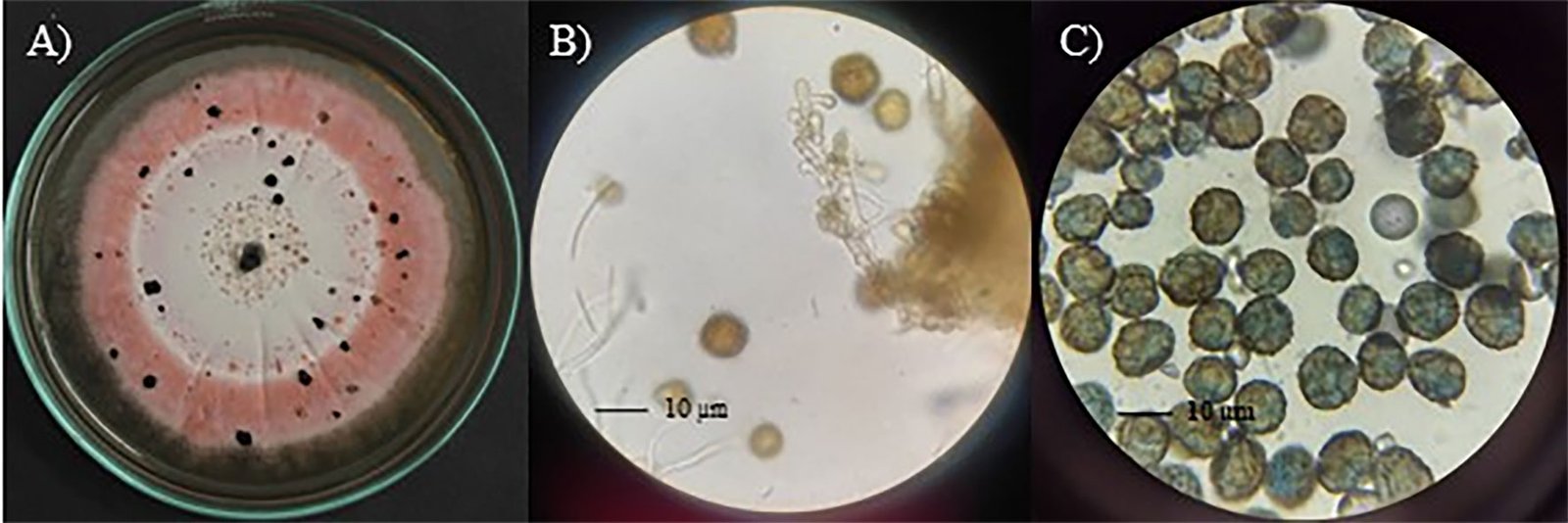
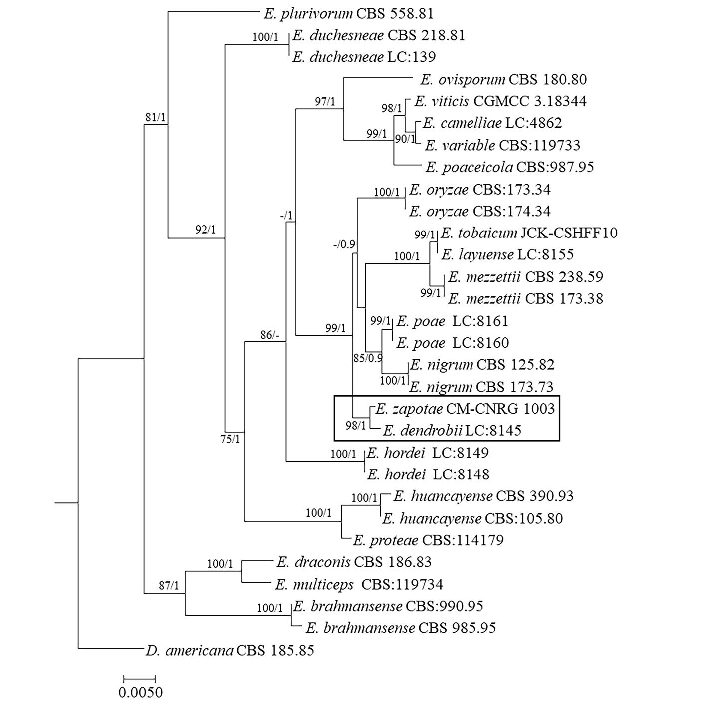
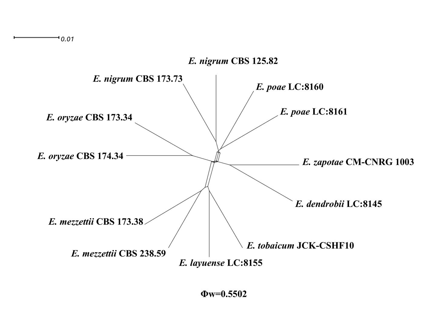
Epicoccum dendrobii exhibits the closest genetic proximity to E. zapotae. Although E. zapotae shares general morphological traits with other Epicoccum species, distinct features support the classification of E. zapotae as a separate species. Conidia of E. dendrobii are multicellular-phragmosporous, verrucose, subglobose-pyriform, brown, with a basal cell, 11-19 µm diam (Chen et al., 2017). In contrast, conidia of E. zapotae are smaller, ranging from 8.84-12.12 µm diam. Additionally, the radial growth rate of E. dendrobii on PDA at 25 °C reaches 34-38 mm diam after 7 days. There is also a significant difference in culture characteristics on PDA between the 2 species, colonies of E. dendrobii display a regular margin, with flat aerial mycelia felty to floccose in texture, white to buff in color, becoming olivaceous near the center (Chen et al., 2017). In contrast, colonies of E. zapotae show slower growth on PDA (31-35 mm) for 7 days and their colonies are distinguished by their intense pink color (Table 4).
Table 4
Comparative morphological characteristics between E. dendrobii and E. zapotae. Data for E. dendrobii adapted from Chen et al. (2017).
| Characteristic | E. dendrobii | E. zapotae |
| Conidia | Multicellular-phragmosporous, verrucose, subglobose-pyriform, brown | Dark pigmented, globose to obovoid with radial separation and a verrucous outer surface |
| Conidial diameter | 11-19 µm | 8.84-12.12 µm |
| Colony margin (PDA) | Regular | Furrowed and circular |
| Aerial mycelium (PDA) | Felty to floccose | Flattened |
| Colony color (PDA) | Beige | Pink |
| Colony diameter (7 days) | 34-38 mm | 31-35 mm |
Epicoccum dendrobii has been reported to cause black leaf spots on Dendrobium fimbriatum (Chen et al., 2017). However, E. zapotae was isolated from sapodilla fruits without visible disease symptoms; therefore, it was probably plant-associated as an endophytic fungus, that can grow asymptomatically within plant tissues (Wen et al., 2022). The ability of endophytic fungi to produce bioactive compounds with biomedical applications has been widely explored (Hashem et al., 2023). In particular, from Epicoccum sp. known as an endophyte of Theobroma cacao, the bioactive compounds epicolactone, epicoccolide A and epicoccolide B have been isolated (Talontsi et al., 2013). Therefore, E. zapotae represents an opportunity for mycochemical studies aimed at exploring the biomedical potential of the bioactive compounds it produced.
Our phylogenetic and morphological analysis, as well as the results from the GCPSR analysis confirm that our isolate, despite its greater genetic proximity to E. dendrobii, presents distinct morphological differences ranging from the size and shape of the conidia to their growth on PDA. This demonstrates that our isolate represents a new species of the genus Epicoccum.
Our comprehensive morphological and molecular analyses have led us to conclude that fungal isolate recovered from the M. zapota fruit, is a new species within the genus Epicoccum which we report as E. zapotae. This discovery represents the first report of E. zapotae isolated from the sapodilla fruits in Veracruz, Mexico, and provides an opportunity for bioprospecting studies aimed at exploring its pharmaceutical potential.
Acknowledgements
This research was supported by Secretaría de Ciencia, Humanidades, Tecnología e Innovación (Secihti), formerly Conahcyt (FORDECYT PRONACES CF/304020 project) and the Universidad Veracruzana (UV-CA-354). L.S.R-G thanks Secihti for the predoctoral grant 802758.
References
Aveskamp, M. M., de Gruyter, J., Woudenberg, J. H. C., Verkley, G. J. M., & Crous, P. W. (2010). Highlights of the Didymellaceae: a polyphasic approach to characterize Phoma and related pleosporalean genera. Studies in Mycology, 65, 1–60. https://doi.org/10.3114/sim.2010.65.01
Barnett, H. L., & Hunter, B. B. (1972). Illustrated genera of imperfect fungi. 3rd Ed. Minneapolis: Burgess Publishing Company.
Benson, D. A., Cavanaugh, M., Clark, K., Karsch-Mizrachi, I., Lipman, D. J., Ostell, J. et al. (2017). GenBank. Nucleic Acids Research, 45, D37–D42. https://doi.org/10.1093/nar/gkw1070
Braga, R., Padilla, G., & Araújo, W. L. (2018). The biotechnological potential of Epicoccum spp.: diversity of secondary metabolites. Critical Reviews in Microbiology, 44, 759–778. https://doi.org/10.1080/1040841X.2018.1514364
Chen, Q., Jiang, J. R., Zhang, G. Z., Cai, L., & Crous, P. W. (2015). Resolving the Phoma enigma. Studies in Mycology, 82, 137–217. https://doi.org/10.1016/j.simyco.2015.10.003
Chen, Q., Hou, L. W., Duan, W. J., Crous, P. W., & Cai, L. (2017). Didymellaceae revisited. Studies in Mycology, 87, 105–159. https://doi.org/10.1016/j.simyco.2017.06.002
Darriba, D., Taboada, G. L., Doallo, R., & Posada, D. (2012). JModelTest 2: More models, new heuristics and parallel computing. Nature Methods, 9, 772. https://doi.org/10.1038/nmeth.2109
Edler, D., Klein, J., Antonelli, A., & Silvestro, D. (2020). raxmlGUI 2.0: a graphical interface and toolkit for phylogenetic analyses using RAxML. Methods in Ecology and Evolution, 12, 373–377. https://doi.org/10.1111/2041-210X.13512
Fávaro, L. C., de Melo, F. L., Aguilar-Vildoso, C. I., & Araújo, W. L. (2011). Polyphasic analysis of intraspecific diversity in Epicoccum nigrum warrants reclassification into separate species. Plos One, 6, e14828. https://doi.org/10.1371/journal.pone.0014828
Gardes, M., & Bruns, T. D. (1993). ITS primers with enhanced specificity for basidiomycetes-application to the identifi-
cation of mycorrhizae and rusts. Molecular Ecology, 2,113–118. https://doi.org/10.1111/j.1365-294X.1993.tb00005.x
Hall, T. A. (1999). BioEdit: a user-friendly biological sequence alignment editor and analysis program for Windows 95/98/NT. Nucleic Acid Symposium Series, 41, 95-98.
Hashem, A. H., Attia, M. S., Kandil, E. K., Fwazi, M. M., Abdelrahman, A. S., Khader, M. S. et al. (2023). Bioactive compounds and biomedical application of endophytic fungi: a recent review. Microbial Cell Factories, 22, 107. https://doi.org/10.1186/s12934-023-02118-x
Huson, D. H. (1998). SplitsTree: analyzing and visualizing evolutionary data. Bioinformatics, 14, 68–73. https://doi.org/10.1093/bioinformatics/14.1.68
Huson, D. H., & Bryant, D. (2006). Application of phylogenetic networks in evolutionary studies. Molecular Biology and Evolution, 23, 254–267. https://doi.org/10.1093/molbev/msj030
Katoh, K., Rozewicki, J., & Yamada, K. D. (2019). MAFFT online service: multiple sequence alignment, interactive sequence choice and visualization. Briefings in Bioinformatics, 20, 1160–1166. https://doi.org/10.1093/bib/bbx108
Kilpatrick, J. A., & Chilvers, G. A. (1981). Variation in a natural population of Epicoccum purpurascens. Transactions of the British Mycological Society, 77, 497–508. https://doi.org/10.1016/S0007-1536(81)80097-6
Lee, A. J., Cadelis, M. M., Kim, S. H., Swift, S., Copp, B. R., & Villas-Boas, S. G. (2020). Epipyrone A, a broad-spectrum antifungal compound produced by Epicoccum nigrum ICMP 19927. Molecules, 25, 5997. https://doi.org/10.3390/molecules25245997
Li, T., Im, J., & Lee, J. (2022). Genetic diversity of Epicoccum nigrum and its effects on Fusarium graminearum. Mycobiology, 50, 457–466. https://doi:10.1080/12298093.2022.2148394
Link, H. F. (1816). Observationes in ordines plantarum naturales III. Magazin der Gesellschaft Naturforschender Freunde Berlin, 7, 37–38.
Liu, D., Coloe, S., Baird, R., & Pedersen, J. (2000). Rapid mini-preparation of fungal DNA for PCR. Journal of Clinical Microbiology, 38, 471. https://doi:10.1128/jcm.38.1.471-471.2000
Maddison, W., & Maddison, D. (2019). Mesquite: a modular system for evolutionary analysis. Version 3.61. https://www.mesquiteproject.org
Müller, J., Müller, K., Neinhuis, C., & Quandt, D. (2010). PhyDE Phylogenetic data editor, version 0.9971. Program distributed by the authors. http://www.phyde.de
Ronquist, F., Teslenko, M., van der Mark, P., Ayres, D. L., Darling, A., Höhna, S. et al. (2012). Mrbayes 3.2: Efficient bayesian phylogenetic inference and model choice across a large model space. Systematic Biology, 61, 539–542. https://doi.org/10.1093/sysbio/sys029
Schol-Schwarz, M. B. (1959). The genus Epicoccum link. Transactions of the British Mycological Society, 42, 149–173. https://doi.org/10.1016/S0007-1536(59)80024-3
Taguiam, J. D., Evallo, E., & Balendres, M. A. (2021). Epicoccum species: ubiquitous plant pathogens and effective biological control agents. European Journal of Plant Pathology, 159, 713–725. https://doi.org/10.1007/s10658-021-02207-w
Talontsi, F. M., Dittrich, B., Schüffler, A., Sun, H., & Laatsch, H. (2013) Epicoccolides: antimicrobial and antifungal polyketides from an endophytic fungus Epicoccum sp. associated with Theobroma cacao. European Journal of Organic Chemistry, 2013, 3174–3180. https://doi.org/10.1002/ejoc.201300146
Taylor, J. W., Jacobson, D. J., Kroken, S., Kasuga, T., Geiser, D. M., Hibbett, D. S. et al. (2000). Phylogenetic species recognition and species concepts in fungi. Fungal Genetics and Biology, 31, 21–32. https://doi.org/10.1006/fgbi.2000.1228
Vilgalys, R., & Hester, M. (1990). Rapid genetic identification and mapping of enzymatically amplified ribosomal DNA from several Cryptococcus species. Journal of Bacteriology, 172, 4238–4246. https://doi.org/10.1128/jb.172.8.4238-4246.1990
Wang, Y., & Guo, L. D. (2004). Morphological and molecular identification of an endophytic fungus Epicoccum
nigrum. Mycosystema, 23, 474–479. https://doi:10.3329/bipt.v29i2.63534
Wen, J., Okyere, S. K., Wang, S., Wang, J., Xie, L., Ran, Y. et al. (2022). Endophytic fungi: an effective alternative source of plant-derived bioactive compounds for pharmacological studies. Journal of Fungi, 8, 205. https://doi.org/10.3390/jof8020205
White, T. J., Bruns, T. D., Lee, S. B., & Taylor, J. W. (1990) Amplification and direct sequencing of fungal ribosomal RNA genes for phylogenetics. In M. A. Innis, D. H. Gelfand, J. J. Sninsky, & T. J. White (Eds.), PCR Protocols: a guide to methods and applications (pp. 315–322). New York: Academic Press. http://dx.doi.org/10.1016/B978-0-12-372180-8.50042-1
Woudenberg, J. H. C., Aveskamp, M. M., de Gruyter, J., Spiers, A. G., & Crous, P. W. (2009). Multiple Didymella teleomorphs are linked to the Phoma clematidina morphotype. Persoonia: Molecular Phylogeny and Evolution of Fungi, 22, 56–62. https://doi.org/10.3767/003158509X427808
Zhang, Z., Schwartz, S., Wagner, L., & Miller, W. (2000). A greedy algorithm for aligning DNA sequences. Journal of Computational Biology, 7, 203–214. https://doi.org/10.1089/10665270050081478

Range extension of Vallonia pulchellaand first record of Valloniacf. excentrica(Gastropoda: Valloniidae) in continental Chile
Extensión del intervalo geográfico de Vallonia pulchella y primer registro de Vallonia cf. excentrica (Gastropoda: Valloniidae) en Chile continental
Marta E. Araya a, Juan A. Aliaga b, Gonzalo Collado c, Juan Francisco Araya d, *
a Sin adscripción, Los Gladiolos 520, Caldera, Chile
b Universidad Tecnológica Metropolitana, Departamento de Química, Las Palmeras 3360, Ñuñoa, Santiago, Chile
c Universidad del Bío-Bío, Facultad de Ciencias, Departamento de Ciencias Básicas, Avenida Andrés Bello 720, Chillán, Chile
d Universidad de Concepción, Programa de Doctorado en Sistemática y Biodiversidad, Barrio Universitario s/n, Concepción, Chile
*Corresponding author: jfaraya@u.uchile.cl (J.F. Araya)
Received: 12 November 2024; accepted: 14 November 2025
Abstract
Non-native mollusk species can have significant ecological and economic impacts on invaded habitats. In recent decades, the number of non-native mollusks in Chile has steadily increased. This study reports the range expansion of Vallonia pulchella (Müller, 1774) and the first record of Vallonia cf. excentrica Sterki, 1893 in the country, using optical microscopy, scanning electron microscopy, and statistical analysis. The first species was found in Caldera (northern Chile) and in La Florida (Santiago, central Chile), while the latter was found only in the last locality. Vallonia pulchella is a potential intermediate host for parasitic worms that can affect local livestock, highlighting the need for sanitary control measures. The discovery of Vallonia cf. excentrica represents the first record of this species in South America.
Keywords:Alien species; Microgastropods; Morphological identification; New records; Terrestrial snails
Resumen
Las especies de moluscos no nativos pueden tener impactos ecológicos y económicos significativos en los hábitats invadidos. En las últimas décadas, el número de moluscos no nativos en Chile ha aumentado de manera constante. Este estudio documenta la expansión del rango de Vallonia pulchella (Müller, 1774) y el primer registro de Vallonia cf. excentrica Sterki, 1893 en el país, utilizando microscopía óptica, microscopía electrónica de barrido y análisis estadístico. La primera especie se encontró en Caldera (norte de Chile) y en La Florida (Santiago, centro de Chile), mientras que la segunda solo en esta última localidad. Vallonia pulchella es un huésped intermediario potencial para gusanos parásitos que pueden afectar al ganado local, lo que resalta la necesidad de medidas de control sanitario. El descubrimiento de Vallonia cf. excentrica representa el primer registro de esta especie en América del Sur.
Palabras clave: Especies exóticas; Microgasterópodos; Identificación morfológica; Nuevos registros; Caracoles terrestres
Introduction
Non-native mollusk species can cause significant ecological and economic impacts on invaded habitats (Darrigran et al., 2020; Lowe et al., 2000; Robinson, 1999; Sylvester & Sardiña, 2015). These species often disrupt local ecosystems by outcompeting native species for resources, altering food webs, and causing declines in biodiversity (Alonso et al., 2025; Collado et al., 2025; Vaughn, 2018). Their ability to rapidly colonize new areas can lead to changes in habitat structure and function, sometimes resulting in the loss of native species that are unable to compete with or adapt to the invaders. In addition, invasive mollusks can introduce new pathogens or parasites that harm local wildlife, livestock, and even humans (Cádiz et al., 2013; Collado et al., 2025).
During the last few decades, the introduction of non-native mollusks in Chile has steadily increased, with recent records of terrestrial and freshwater species on Easter Island and especially in the central region of the country (e.g., Cádiz & Gallardo, 2007; Cádiz et al., 2013; Collado, 2014, 2017; Darrigran et al., 2020; Kirch et al., 2009; Letelier et al., 2007). The number of non-native mollusks in Chile has grown from 13 species (Valdovinos-Zarges, 1999) to 34 species (Araya, 2015), including marine, freshwater, and terrestrial species. Of these, 20 are ground-dwelling terrestrial mollusks, making this the largest informal group of invasive species in any South American country, with numbers similar to those found in Argentina (Virgillito & Miquel, 2013). Most of these introduced species have a European origin, and some are known to negatively impact endemic biota, often by competing with or preying on native species, or acting as hosts for various parasites (Cádiz et al., 2013). Prevention and continuous monitoring are therefore essential to avoid the introduction and establishment of additional non-native species in new ecosystems.
In the present study, as part of an ongoing investigation on the diversity of terrestrial mollusks in Chile (Araya, 2016; Araya & Aliaga, 2015; Miquel & Araya, 2013, 2015), we report the range extension of Vallonia pulchella (Müller, 1774) and the first record of Vallonia cf. excentrica Sterki, 1893 in continental Chile. The Global Biodiversity Information Facility (GBIF, 2024) database had previously reported V. pulchella in Easter Island, as well as in Caldera and Coquimbo in continental Chile (unpublished data). Vallonia pulchella, the lovely Vallonia, is Holarctic in origin (Hotopp et al., 2013) and has been documented as an introduced species in South Africa, Madagascar, Australia, New Zealand and several other Asian countries (Gerber, 1996; Herbert, 2010; Mitra et al., 2005; Robinson, 1999; Roll et al., 2009; Stanisic, 1998), as well as in Argentina, Brazil, Peru, and Uruguay in South America (Rumi et al., 2010; Virgillito & Miquel, 2013). In Chile, the species was first reported as introduced by Philippi (1885) from the area surrounding Santiago. Later, Lataste (1896, fide Porter, 1926) found this species in Linderos, south of Santiago. More recently, it was reported by PNUD (2014), although the specific location was not detailed. On the other hand, V. cf. excentrica, another Holartic species (Metcalf, 1984; Nekola, 2002), is reported here for the first time as an introduced species in the country and in South America.
Materials and methods
Snail specimens were hand-collected from wet soil in 2017 in 2 urban areas of continental Chile: Caldera in the north and La Florida in Santiago City, in the central region of the country. Snails were sorted out from 2 soil samples of about 500 g in each location. Adult specimens were photographed using a Motic SMZ-168 stereomicroscope equipped with a Moticam 2000 digital camera and measured with a millimeter ruler. Specimens were also examined using a Hitachi SU3500 scanning electron microscope (SEM). Prior to observation, the snails were immersed in a dilute sodium hypochlorite solution for 3 minutes, rinsed in distilled water, and air-dried.
Species identification was based on original descriptions and additional literature (Burch & Jung, 1988; Herbert, 2010; Sterki, 1893). To assess morphometric variation among introduced populations, we measured 6 shell variables: shell length (SL), shell width (SW), shell height (SH), aperture height (AH), aperture width (AW), and the distance from the umbilicus to the last body whorl (UBW). The data were log-transformed to assess normality and homoscedasticity. Since some variables did not meet these assumptions, we applied the nonparametric Mann-Whitney U test (M-W U) using PAST software V. 4.13 (Hammer et al., 2001). Additionally, we performed a principal component analysis (PCA) in PAST to investigate whether shell shape variation could distinguish between the 2 morphologically similar species in morphometric space. This analysis included 14 individuals from Caldera and 13 from La Florida assigned to V. pulchella, and 3 individuals assigned to V. cf. excentrica. Specimens from Caldera and La Florida smaller than 2 mm were excluded from the analysis. Voucher specimens were deposited in the Museo de Ciencias Naturales Profesor Pedro Ramírez Fuentes (MCNPPRF), Chillán, Chile, and the Laboratorio de Malacología y Sistemática Molecular, Universidad del Bío-Bío, Chillán, Chile (LMSM) (see Results).
Results
Stereomicroscope and SEM observations revealed the presence of 2 non-native species of the genus Vallonia in continental Chile (Figs. 1-4).
Phylum Mollusca Linnaeus, 1758
Class Gastropoda Cuvier, 1797
Superfamily Pupilloidea W. Turton, 1831
Family Valloniidae E. S. Morse, 1864
Genus Vallonia Risso, 1826
Vallonia pulchella (Müller, 1774)
Figs. 1A-K, 3A
Material examined. 17 specimens from Caldera (27°04’ S, 70°49’ W) (LMSM 1-17), 18 specimens from La Florida (33°27’ S, 70°40’ W) (MCNPPRF 139–24, MCNPPRF 139-25, LMSM 3-18).
Morphology. Shell with 3 1/8 whorls, fine axial striae (Fig. 1A, D, I), depressed, umbilicated, gray-white or corneous, translucent with a matte gloss. Adult shell diameter: 1.6-2.6 mm (Caldera), 1.3-2.4 mm (La Florida). Protoconch smooth (620 µm), with 1 1/8 whorls and a clear transition to the teleoconch (Fig. 3A). Round umbilicus (Fig. 1C, F, K), about 1/4 of the shell diameter. Near-circular aperture, slightly oblique (Fig. 1B, E, G, H, J), translucent peristome with a thickened lip in adults.
Remarks
Vallonia pulchella resembles Vallonia excentrica. Some authors consider V. excentrica to be a form of V. pulchella (Adams, 1906; Hubendick, 1950). Korte and Armbruster (2003) suggest that V. excentrica is paraphyletic, within the same clade as V. pulchella. However, V. pulchella can be distinguished by a higher spire, a less elongated umbilicus, and a translucent, thickened lip (in contrast, the lip of V. excentrica is white) (Sterki, 1893).
Vallonia cf. excentrica Sterki, 1893
Figs. 2A-F, 3B
Material examined. 3 specimens from La Florida (33°27’ S, 70°40’ W) (LMSM 1-3).
Morphology. Shell with about 3 1/8 whorls, fine axial striae (Fig. 2A-F), highly depressed, widely umbilicated, whitish or corneous, translucent. Adult size: 1.8-2.1 mm. Protoconch smooth (810 µm), 1 1/4 whorls (Fig. 3B), with clear transition to teleoconch. Round umbilicus (Fig. 2C, F), ~ 1/4 shell diameter. Subcircular to crescentic aperture, slightly oblique (Fig. 2B, E, J), thin lip.
Remarks
Vallonia excentrica is distinguished from V. pulchella by its larger protoconch (Fig. 3), lower spire, and sharp, smooth aperture lip (thickened in V. pulchella). The crescentic aperture and the absence of radial sculpture of ribs distinguishes this species from all other Vallonia species.
No statistical differences were found between V. pulchella populations from Caldera and La Florida in any shell variable (M-W U test: p > 0.05) (Table 1). The first 2 principal components (PCAs) explained 90.02% of the variation (PC1: 84.7%, PC2: 5.3%). Populations of V. pulchella exhibited substantial overlap in morphometric space but were clearly separated from V. cf. excentrica specimens (Fig. 4).
Discussion
In the present study, we report a range extension of V. pulchella and the first documented occurrence of V. cf. excentrica in Chile and South America. The statistical analyses confirmed our typological assignment of snails from Caldera and La Florida to V. pulchella. There were no significant differences in any shell variables between the 2 samples, and in morphometric space, individuals from both localities clustered as a single group. Moreover, the analysis revealed that these specimens are clearly separated from those assigned to V. cf. excentrica, supporting their distinction as separate species.
Previous records of V. pulchella from Chile refer to preserved specimens from Bosque de Ceibos, Anakena, housed in the Field Museum of Natural History (FMNH 312411 and 312412), Arlington, Virginia (unpublished data). In addition, samples from Coquimbo were identified by Bernhard Hausdorf (iNaturalist 42089250), and those from Caldera are preserved in the Museu de Ciències Naturals de Barcelona (MCNB-Malac MZB 89-0910) (GBIF, 2024).
Although Vallonia species have low vagility, they can be dispersed by birds, fish, water and human activities (Altaba, 2015; Boycott, 1934), in the latter case through the unintentional transport of plants, soil, or leaf litter (Schembri & Lanfranco, 1996). However, the means of introduction of Vallonia species to Chile remains unknown, as does the origin of the samples from Easter Island, Caldera, and Coquimbo. Their introduction into the country is most likely associated with human activity, given that both Caldera and Coquimbo are very active ports and Easter Island has a high influx of tourism. Due to the species’ wide distribution in Chile, a single introduction event seems unlikely.
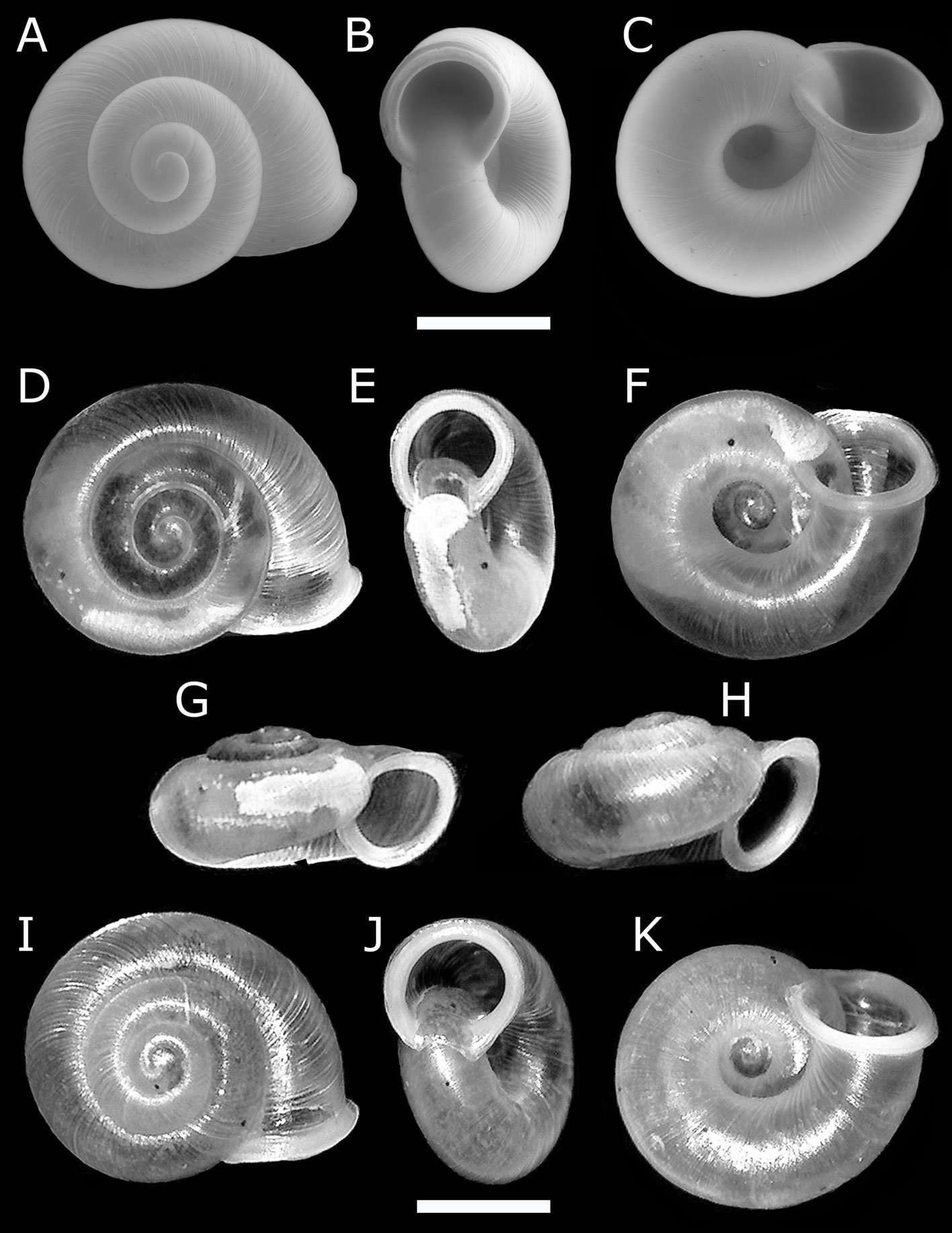
Although we did not estimate the abundance of V. pulchella at the sampled sites, previous studies have reported densities ranging from fewer than 10 individuals/m² (Čejka & Hamerlik, 2009; Koralewska-Batura & Błoszyk, 2007) to up to 588 individuals/m² (Hermida et al., 1993). While we recorded only 3 individuals of V. cf. excentrica, this would represent the first record of the species as introduced in South America. However, this species has already been introduced to South Africa, Australia, and a great part of New Zealand (Barker, 1999).
Vallonia species are similar in size and shape (Gerber & Bössneck, 2009; Sterki, 1893). However, although V. pulchella and V. cf. excentrica are morphologically similar, they differ in the shape of the peristome lip, reflected and thickened in V. pulchella, but thin in the present V. excentrica specimens, and in protoconch size, which is larger in the latter species.
As an invasive species, V. pulchella could threaten livestock, particularly sheep and rabbits, as an intermediate host for nematodes such as Protostrongylus boughtoni (Goble & Dougherty, 1943), P. hobmaieri (Schulz et al., 1933), P. rufescens (Leuckart, 1865), and Varestrongylus pneumonicus (Bhalerao, 1932) (Grewal et al., 2003; Samson & Holmes, 1985). Continuous monitoring is essential to assess its spread. Due to its small size, adults, juveniles, and eggs, V. pulchella can be easily transported in soil and potted plants. Its iteroparous mode of reproduction and ability to self-fertilize could further contribute to its dispersal (Kuźnik-Kowalska & Proćków, 2016; Whitney, 1941). Given that most specimens were collected from plant litter and pots, the nursery trade could act as a dispersal vector, as seen with other small invasive snails (Forsyth, 2015).
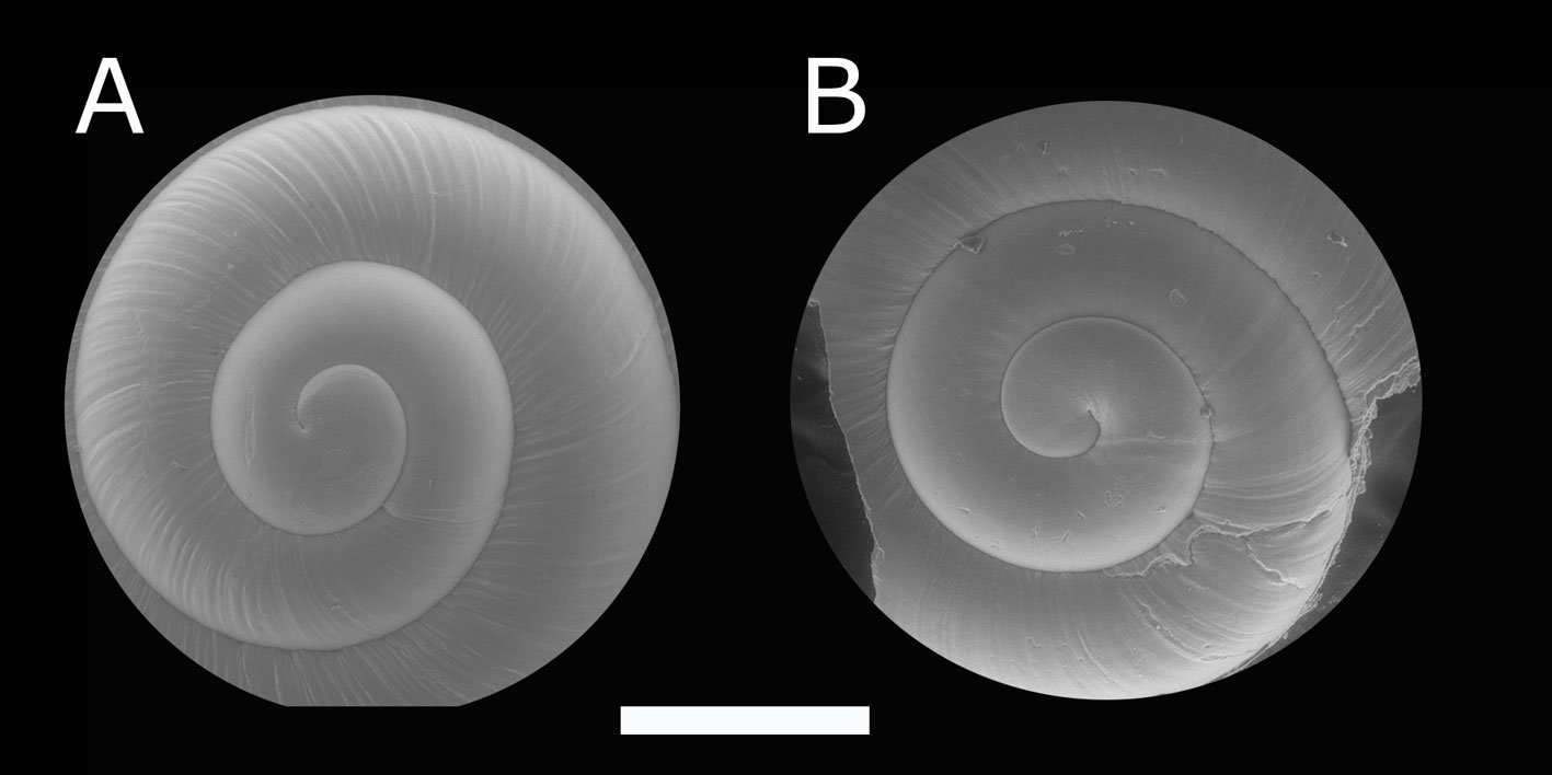
The small size of Vallonia species may explain the limited number of records, as small non-native snails are often recognized only long after they have arrived (Hutchinson et al., 2014). The new records presented in this study extend the known distribution of V. pulchella in South America and provide the first documented record of V. cf. excentrica in Chile and South America. However, these species are probably present elsewhere in the country, especially in the central region, where human population density is higher.
Table 1
Mann-Whitney U test results between Vallonia pulchella specimens collected in Caldera (northern Chile) and La Florida (central Chile). Shell length (SL), shell height (SH), shell width (SW), aperture height (AH), aperture width (AW), body whorl length (BWL), and the distance from the umbilicus to the last body whorl (UBW). Standard deviation: S.D.
| Shell variable | Caldera (n) | Mean (±S.D.) | La Florida (n) | Mean (±S.D.) | U | p-value |
| SL | 14 | 2.3 (± 0.2) | 13 | 2.2 (± 0.1) | 72.0 | 0.3549 |
| SH | 14 | 1.8 (± 0.1) | 13 | 1.8 (± 0.1) | 87.5 | 0.8736 |
| SW | 14 | 1.1 (± 0.1) | 13 | 1.0 (± 0.1) | 79.0 | 0.5483 |
| AH | 14 | 1.0 (± 0.1) | 13 | 1.0 (± 0.1) | 79.0 | 0.5358 |
| AW | 14 | 1.0 (± 0.1) | 13 | 1.0 (± 0.1) | 75 | 0.4097 |
| UBW | 14 | 1.3 (± 0.1) | 13 | 1.2 (± 0.1) | 73 | 0.3453 |
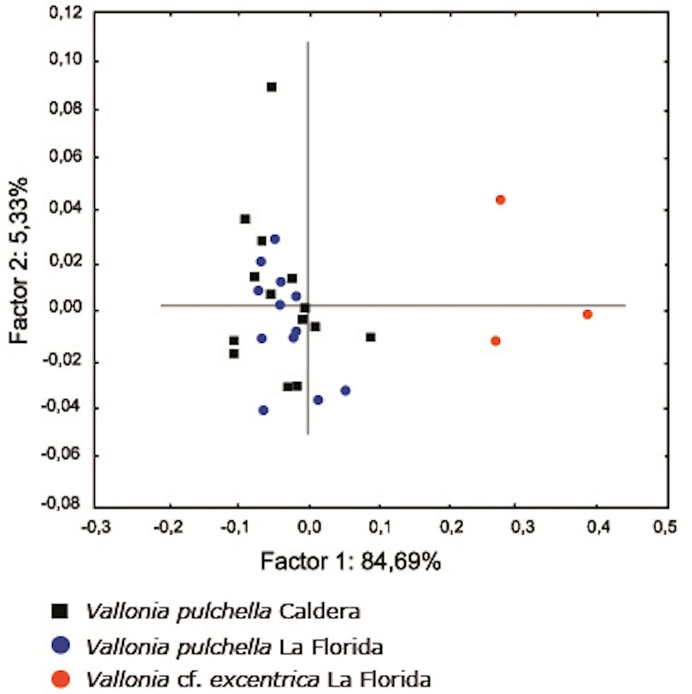
It is also important to note that, although V. pulchella and V. cf.excentrica have been considered conspecific by some authors (e.g., Sterki, 1893), our study demonstrates that they are distinct species, based on clear morphological differences, particularly in the form of the lip and protoconch. Nevertheless, a comprehensive and integrative taxonomic revision of both species is still needed to fully resolve their relationship.
Acknowledgments
We thank Cristian Suárez for assistance with the SEM observations. We also thank FONDEQUIP Program (No. EQM-140088) and the anonymous reviewers. JFA also acknowledges the ANID doctoral fellowship 21180344, which supported the first 2 years of his doctoral studies.
References
Adams, L. E. (1906). Vallonia costata + excentrica. Journal of Conchology, 11, 364–365.
Alonso, Á., Collado, G. A., Gérard, C., Levri, E. P., Salvador, R. B., & Castro-Díez, P. (2025). Effects of the invasive aquatic snail Potamopyrgus antipodarum (Gray, 1853) on ecosystem properties and services. Hydrobiologia, 852, 1339–1357. https://doi.org/10.1007/s10750-022-05116-z
Altaba, C. R. (2015). Once a land of big wild rivers: specialism is context-dependent for riparian snails (Pulmonata: Valloniidae) in central Europe. Biological Journal of the Linnean Society, 115, 826–841. https://doi.org/10.1111/bij.12546
Araya, J. F. (2015). Current status of the non-non-native molluscs in Chile, with the first record of Otala punctata (Müller, 1774) (Gastropoda, Helicidae) in the country and new records for Cornu aspersum (Müller, 1774) and Deroceras laeve (Müller, 1774). Journal of Natural History, 49, 1731–1761. https://doi.org/10.1080/00222933.2015.1006703
Araya, J. F. (2016). On some land snails (Mollusca: Gastropoda) of Los Molles, central Chile. Revista Mexicana de Biodiversidad, 87, 1365–1368. https://doi.org/10.1016/j.rmb.2016.10.002
Araya, J. F., & Aliaga, J. A. (2015). A new species of Lilloiconcha Weyrauch,1965 (Pulmonata: Charopidae) from central Chile. Zootaxa, 4007, 295–297. https://doi.org/10.11646/zootaxa.4007.2.13
Barker, G. M. (1999). Naturalised terrestrial Stylommato-phora (Mollusca: Gastropoda). Fauna of New Zealand,
38, 1–253. https://doi.org/10.7931/J2/FNZ.38
Boycott, A. E. (1934). The habitats of land Mollusca in Britain. Journal of Ecology, 22, 1–38. https://doi.org/10.2307/2256094
Burch, J. B., & Jung, Y. (1988). Land snails of the University of Michigan Biological Station area. Walkerana, 3, 1–177.
Cádiz, F. J., & Gallardo, C. S. (2007). Arion intermedius (Gastropoda: Stylommatophora); first record of this introduced slug in Chile, with notes on its anatomy and natural history. Revista Chilena de Historia Natural, 80, 99–108.
Cádiz, F. J., Cádiz, D. G., & Grau, J. H. (2013). An invasive predatory snail Oxychilus alliarius (Miller, 1822) (Stylommatophora: Zonitidae) threatens the native malacofauna of continental Chile: a morphological and molecular confirmation. Studies on Neotropical Fauna and Environment,48, 119–124. https://doi.org/10.1080/01650521.2013.843910
Čejka, T., & Hamerlik, L. (2009). Land snails as indicators of soil humidity in Danubian woodland (SW Slovakia). Polish Journal of Ecology, 57, 741–747.
Collado, G. A. (2014). Out of New Zealand: molecular identification of the highly invasive freshwater mollusk Potamopyrgus antipodarum (Gray, 1843) in South America. Zoological Studies, 53, 70. https://doi.org/10.1186/s40555-014-0070-y
Collado, G. A. (2017). Unraveling cryptic invasion of a fresh-water snail in Chile based on molecular and morphological data. Biodiversity and Conservation,26, 567–578. https://doi.org/10.1007/s10531-016-1255-y
Collado, G. A., Cristina, D., Darrigran, G., & Alonso Á. (2025). Attributes and effects of the invasive air-breathing freshwater snail Physa acuta on ecosystem properties and services. Marine and Freshwater Research, 76, MF25023. https://doi.org/10.1071/MF25023
Darrigran, G., Agudo-Padrón, I., Baez, P., Belz, C., Cardoso, F., Carranza, A. et al. (2020). Non-native mollusks throughout South America: emergent patterns in an understudied continent. Biological Invasions, 22, 853–871. https://doi.org/10.1007/s10530-019-02178-4
Forsyth, R. G. (2015). First record of Carychium minimum Müller, 1774 in New Brunswick, Canada (Mollusca: Gastropoda: Ellobioidea). Check List, 11, 1511. https://doi.org/10.15560/11.1.1511
Gerber, J. (1996). Revision der Gattung Vallonia Risso, 1826 (Mollusca: Gastropoda: Valloniidae). Schriften zur Malakozoologie aus dem Haus der Natur-Cismar, 8, 1–227.
Gerber, J., & Bössneck, U. (2009). The genus Vallonia in Nepal: (Gastropoda: Pulmonata: Valloniidae). Archiv für Molluskenkunde, 138, 43–52. https://doi.org/10.1127/arch.moll/0003-9284/138/043-052
GBIF (2024). Global Biodiversity Information Facility. Retrieved November 10, 2024 from: https://www.gbif.org/es/species/2296010
Grewal, P. S., Grewal, S. K., Tan, L., & Adams, B. J. (2003). Parasitism of molluscs by nematodes: types of associations and evolutionary trends. Journal of Nematology, 35, 146–156.
Hammer, Ø., Harper, D. A. T., & Ryan, P. D. (2001). PAST: paleontological statistics software package for education and data analysis. Palaeontologia Electronica, 4, 9.
Herbert, D. G. (2010). The introduced terrestrial Mollusca of South Africa. SANBI Biodiversity Series 15. Pretoria: South African National Biodiversity Institute.
Hermida, J., Outeiro, A., & Rodríguez, T. (1993). Aspectos ecológicos de Vallonia pulchella (Muller, 1774) (Gastropoda, Pulmonata). Nova Acta Científica Compostelana (Bioloxía), 4, 129–135.
Hotopp, K. P., Pearce, T. A., Nekola, J. C., Slapcinsky, J., Dourson, D. C., Winslow, M. et al. (2013). Land snails and slugs of the Mid-Atlantic and Northeastern United States. Pittsburgh, PA: Carnegie Museum of Natural History. Retrieved November 10, 2024 from: https://www.carnegiemnh.org/science/mollusks/index.html
Hubendick, B. (1950). The validity of Vallonia excentrica Sterki. Proceedings of the Malacological Society of London, 28, 75–78. https://doi.org/10.1093/oxfordjournals.mollus.a064569
Hutchinson, J., Reise, H., & Robinson, D. (2014). A biography of an invasive terrestrial slug: the spread, distribution and habitat of Deroceras invadens. NeoBiota, 23, 17–64. https://doi.org/10.3897/neobiota.23.7745
Kirch, P., Christensen, C., & Steadman, D. (2009). Subfossil land snails from Easter Island, including Hotumatua anakenana, new genus and species (Pulmonata: Achatinellidae). Pacific Science,63, 105–122. https://doi.org/10.2984/15346188(2009)63[105:SLSFEI]2.0.CO;2
Koralewska-Batura, E., & Błoszyk, J. (2007). Stability of malacocoenoses in an ash-elm forest based on two-year observations. Folia Malacologica, 15, 175–180. https://doi.org/10.12657/folmal.015.015
Korte, A., & Armbruster, G. F. J. (2003). Apomorphic and plesiomorphic ITS-1 rDNA patterns in morphologically similar snails (Stylommatophora: Vallonia), with estimates of divergence time. Journal of Zoology, 260, 275–283. https://doi.org/10.1017/S0952836903003741
Kuźnik-Kowalska, E., & Proćków, M. (2016). Reproductive biology and growth of two Vallonia species in laboratory conditions (Gastropoda: Eupulmonata: Valloniidae). Folia Malacologica, 24, 265–273. https://doi.org/10.12657/folmal.024.022
Lataste, F. (1896). L’ Helix pulchella dans les vignes de Linderos. Santiago: Actes de la Societé Scientifique du Chili. Tome VI.
Letelier, S., Ramos, A., & Huaquín, L. (2007). Moluscos dulceacuícolas exóticos en Chile. Revista Mexicana de Biodiversidad, 78, 9–13. https://doi.org/10.22201/ib.20078706e.2007.002.301
Lowe, S., Browne, M. & Boudlejas, S. (2000). 100 of the world’s worst invasive alien species. A selection from the Global Invasive Species Database. The Invasive Species Specialist Group (ISSG), a specialist group of the Species Survival Commission (SSC) of the World Conservation Union (IUCN), Auckland, New Zealand.
Metcalf, A. L. (1984). Distribution of land snails of the San Andres and Organ Mountains, Southern New Mexico. The Southwestern Naturalist, 29, 35–44. https://doi.org/10.2307/3670767
Miquel, S. E., & Araya, J. F. (2013). A new Charopidae from Chile and Argentina, Stephacharopa calderaensis n. gen. and n. sp., with remarks on the taxonomy of the genus Stephadiscus Hylton Scott 1981 (Mollusca: Gastropoda Pulmonata). Archiv für Molluskenkunde, 142, 227–235. https://doi.org/10.1127/arch.moll/1869-0963/142/227-235
Miquel, S. E., & Araya, J. F. (2015). New records of terrestrial molluscs of the Juan Fernández Archipelago (Chile), with the description of a new genus and species of Charopidae (Gastropoda Stylommatophora). Archiv für Molluskenkunde, 144, 155–167. https://doi.org/10.1127/arch.moll/1869-0963/144/155-167
Mitra, S. C., Dey, A., & Ramakrishna. (2005). Pictorial handbook. Indian land snails. Kolkata: Zoological Survey of India.
Nekola, J. C. (2002). Large-scale terrestrial gastropod community composition patterns in the Great Lakes
region of North America. Diversity and Distributions, 9, 55–71. https://doi.org/10.1046/j.1472-4642.2003.00165.x
Philippi, R. A. (1885). Zoolojía. Sobre los animales introducidos en Chile desde su conquista por los españoles. Anales de la Universidad de Chile, 67, 319–335.
PNUD (Programa de las Naciones Unidas para el Desarrollo). (2014). Moluscos invasores de Chile. Documento del Taller Moluscos exóticos invasores en Chile: efectos en la biodiversidad. Santiago de Chile: Programa de las Naciones Unidas para el Desarrollo.
Porter, C. (1926). Los estudios malacológicos en Chile. Revista Chilena de Historia Natural, 30, 26–39.
Robinson, D. G. (1999). Alien invasions: the effects of the global economy on non-marine gastropod introductions into the United States. Malacologia, 41, 413–438.
Roll, U., Dayan, T., Simberloff, D., & Mienis, H. K. (2009). Non-indigenous land and freshwater gastropods in Israel. Biological Invasions, 11, 1963–1972. https://doi.org/10.1007/s10530-008-9373-4
Rumi, A., Sánchez, J., & Ferrando, N. S. (2010). Theba pisana (Müller, 1774) (Gastropoda, Helicidae) and other alien land molluscs species in Argentina. Biological Invasions, 12, 2985–2990. https://doi.org/10.1007/s10530-010-9715-x
Samson, J., & Holmes, J. C. (1985). The effect of temperature on rates of development of larval Protostrongylus spp. (Nematoda: Metastrongyloidea) from bighorn sheep, Ovis canadensis canadensis, in the snail Vallonia pulchella. Canadian Journal of Zoology, 63, 1445–1448. https://doi.org/10.1139/z85-215
Schembri, P. J., & Lanfranco, E. (1996). Introduced species in the Maltese Islands. In A. E. Baldacchino, & A. Pizzuto (Eds.), Introduction of alien species of flora and fauna. Proceedings of a seminar held at Qawra, Malta (pp. 29–54). Floriana, Malta: Environment Protection Department.
Stanisic, J. (1998). Family Valloniidae. In P. L. Beesley, G. J. B. Ross, & A. Wells (Eds.), Mollusca: the southern synthesis. Part B. Fauna of Australia, Vol. 5 (pp. 1085–1086). Melbourne: CSIRO Publishing.
Sterki, V. (1893). Observations on Vallonia. Proceedings of the Academy of Natural Sciences of Philadelphia, 45, 234–279.
Sylvester, F., & Sardiña, P. (2015). Relationships of Limnoperna fortunei with benthic animals. In D. Boltovskoy (Ed.), Limnoperna fortunei: the ecology, distribution and control of a swiftly spreading invasive fouling mussel (pp. 191–210). Cham: Springer International Publishing.
Valdovinos-Zarges, C. (1999). Biodiversidad de moluscos chilenos: base de datos taxonómica y distribucional. Gayana, 63, 111–164.
Vaughn, C. C. (2018). Ecosystem services provided by fresh-water mussels. Hydrobiologia, 810, 15–27. https://doi.org/10.1007/s10750-017-3139-x
Virgillito, M., & Miquel, S. E. (2013). New records of exotic land snails and slugs in Argentina. Revista del Museo Argentino de Ciencias Naturales, Nueva Serie, 15, 295–303.
Whitney, M. E. (1941). The hermaphrodite gland and germ cells of Vallonia pulchella Müll. Michigan Academy of Science, 26, 311–338.

Morphological description of the first zoea of the freshwater shrimp Macrobrachium crenulatum (Decapoda: Palaemonidae) and a comparison to its congeners in the Neotropics
Descripción morfológica de la primera zoea del camarón de agua dulce Macrobrachium crenulatum (Decapoda: Palaemonidae) y una comparación con sus congéneres del Neotrópico
Lucas Oliveira-Rogeri a, *, Rodrigo Pantoni a, Ingo S. Wehrtmann b, c, d, Fernando L. Mantelatto a, João Alberto Farinelli Pantaleão e
a University of São Paulo, Faculty of Philosophy, Science and Letters at Ribeirão Preto, Department of Biology, Laboratory of Bioecology and Crustacean Systematics, Av. Bandeirantes, 3900, 14040-901, Ribeirão Preto, São Paulo, Brazil
b Universidad de Costa Rica, Unidad de Investigación Pesquera y Acuicultura, Centro de Investigación en Ciencias del Mar y Limnología, 11501-2060 San José, Costa Rica
c Universidad de Costa Rica, Centro de Investigación en Biodiversidad y Ecología Tropical, Museo de Zoología, 11501-2060 San José, Costa Rica
d Universidad del Valle de Guatemala, Editorial Universitaria, 18 Avenida 11-95, Zonas 15, Vista Hermosa III, Ciudad de Guatemala, Guatemala
e Federal University of Alagoas, Institute of Biological and Health Sciences, Laboratory of Bioecology and Development of Crustaceans, Av. Paulo Holanda, 143, 57072-970, Maceió, Alagoas, Brazil
*Corresponding author: luquinhaor.bio55@usp.br (L. Oliveira-Rogeri)
Received: 08 April 2025; accepted: 13 November 2025
Abstract
We present the first description of Zoea I of Macrobrachium crenulatum and compare it with available data of other zoeae of Macrobrachium spp. of the Neotropics to identify morphological characteristics to differentiate the first zoea of M. crenulatum from zoeae of other species of the genus. A female with embryos was collected in the Atlantic drainage of Costa Rica, Central America. After hatching in the laboratory, larvae were preserved in glycerinate alcohol and later semi-permanent slides were prepared for morphological study and larval description. A table was prepared to compare the morphology of the first zoea of M. crenulatum to the first zoeae of other species of Macrobrachium. Among species of Macrobrachium phylogenetic and geographically closely related, the first zoea of M. crenulatum can be differentiated by the comparison of some structures as antenna (number of articles on scaphocerite), maxillipeds (number of plumose setae; setation pattern), maxilla (setation pattern), maxillule (number of spines), and telson (outer pair of setae). The larval morphology of M. crenulatum corroborated the phylogenetic position and may serve as a taxonomic tool for the distinction between the first zoea of closely related species.
Keywords: Atlantic drainage; Caridea; Costa Rica; Larval morphology
Resumen
Presentamos la primera descripción de la zoea I de Macrobrachium crenulatum y la comparamos con datos disponibles de otras primeras zoeas de especies de Macrobrachium del Neotrópico, con el objetivo de identificar características morfológicas que permitan diferenciar la primera zoea de M. crenulatum respecto de las de otras especies del género. Una hembra ovígera fue colectada en la cuenca atlántica de Costa Rica, Centroamérica. Tras la eclosión en laboratorio, las larvas fueron preservadas en alcohol glicerinado y, posteriormente, se prepararon láminas semipermanentes para su estudio morfológico y la descripción larval. Se elaboró una tabla comparativa con la morfología de la primera zoea de M. crenulatum respecto de las primeras zoeas de otras especies de Macrobrachium. Entre las especies filogenética y geográficamente relacionadas, la zoea I de M. crenulatum puede distinguirse mediante la comparación de estructuras como antenas (número de artejos del escafocerito), maxilípedos (número y patrón de setas plumosas), maxila (patrón de setas), maxílula (número de espinas) y telson (disposición del par lateral de setas marginales). La morfología larval de M. crenulatum respalda su posición filogenética y puede servir como herramienta taxonómica para diferenciar la primera zoea de especies estrechamente relacionadas.
Palabras clave: Vertiente Atlántica; Caridea; Costa Rica; Morfología larvaria
Introduction
The genus Macrobrachium Spence Bate, 1868 is one of the most speciose taxa among caridean shrimps, currently accounting for more than 270 species (De Grave & Fransen, 2011; Pantaleão et al., 2025; Poore & Ahyong, 2023). The genus is cosmopolite, with representatives inhabiting different environments with distinct climate conditions throughout the world. Macrobrachium is remarkably diverse in subtropical and tropical regions, such as Central and South America as well as in the Indo-Pacific region (Murphy & Austin, 2005; Pileggi & Mantelatto, 2012; Pileggi et al., 2014). Some species of Macrobrachium are marine, estuarine and anchialine, but the vast majority inhabit typically freshwater systems, such as rivers, lakes and floodplains (Chace & Bruce, 1993; Fujita et al., 2015; Poore & Ahyong, 2023).
Besides the elevated number of species, the genus is highly diverse in terms of morphological characteristics, ecological traits and reproductive strategies (Sastry, 1983; Wowor et al., 2009). Some species of Macrobrachium, for instance, complete their entire life cycle in freshwater. Others are amphidromous and depend on both freshwater and estuarine/marine environments to finish their cycle, which implies migration events from one water system to the other (Bauer, 2011a, b; Liu et al., 2007; Wowor et al., 2009). Another varying feature of the biology and ecology of species of Macrobrachium is the duration of larval development. While some species have extended larval development (ELD) with a long duration of the larval period and the number of larval stages varying between 9 and 13, others have an abbreviated larval development (ALD) with 1 or 2 free-swimming larval stages before reaching the juvenile stage (Anger, 2013; Jalihal et al., 1993; Shokita, 1985; Wowor et al., 2009).
One of the representatives of this shrimp genus is Macrobrachium crenulatum Holthuis, 1950, with its geographical distribution including the coastal waters of Nicaragua, Costa Rica, Panama, Colombia, Venezuela, Jamaica, Grenada, and Trinidad and Tobago (Holthuis, 1952; Hunte, 1979; Pileggi et al., 2014; Rossi, 2012). This species is characterized by an amphidromous life cycle with extended larval development (ELD) (Bauer, 2013; Pileggi et al., 2014). Adults have been the target of taxonomic, ecological and molecular studies (Pileggi et al., 2014; Rossi, 2012; Valencia & Campos, 2007); however, the larval morphology of M. crenulatum has never been described. This lack of information about the larval morphology hinders the global comprehension of species, since understanding larval features is not only useful for the larval recognition itself, but also for studies about the larval ecology, for resolving taxonomic problems and for providing phylogenetic insights (Lai et al., 2013; Pantaleão et al., 2025).
Pileggi et al. (2014) conducted a molecular study, which provided phylogenetic data about the “sibling species” of Macrobrachium from Central America. According to these authors, morphological features of adults are often not sufficient to distinguish the “sibling species” of the genus, including the distinction between transisthmian pairs of sibling species Macrobrachium hancocki Holthuis, 1950 and M. crenulatum. Recently, Pantaleão et al. (2025) conducted a novel study integrating larval morphology and molecular data to understand the phylogenetic context of relevant traits of species of Macrobrachium life history and larval morphology. Nonetheless, the authors highlighted that one of the limitations was the lack of larval descriptions for the vast majority of species of Macrobrachium as well as the accuracy of the available descriptions.
Considering the high diversity of Macrobrachium in Central America, the absence of larval descriptions hinders the identification of their larvae in plankton samples and thus a broader understanding of their larval ecology, especially in river systems where several species of Macrobrachium co-occur (see Lara & Wehrtmann, 2011). Therefore, here we describe for the first time the first zoea of M. crenulatum. The results include a comparison with other newly hatched larvae of species of Macrobrachium, which may serve as a taxonomic tool for the distinction between the first zoeae of these closely related species.
Materials and methods
An ovigerous female (carapace length = 16.6 mm) was collected on 23 May 2010 in the Suarez River (09º43’40” N, 22º50’25.5” W), at the district of Cahuita, in the province of Limón, in the Atlantic drainage of Costa Rica, Central America. The female was collected using a sieve through ascendant movements near the margins of the river; once obtained, it was moved to the laboratory where it was kept alive until the larvae hatched 1 day after the collection. The hatching larvae were collected using a Pasteur pipette and then transferred to a tube containing glycerinate alcohol 80% (1:1). The parental female was preserved in alcohol 80%. Both larvae and the female were deposited at the Coleção de Crustáceos do Departamento de Biologia (CCDB), Faculdade de Filosofia, Ciências e Letras de Ribeirão Preto (FFCLRP), Universidade de São Paulo (USP). Genetic sequences of the parental female were generated by Rossi and Mantelatto (2013) and are available in GenBank under accession numbers JQ805902 for the cytochrome c oxidase subunit I (COI) and JQ805867 for the histone 3 (H3) markers (https://www.ncbi.nlm.nih.gov/nuccore/jq805902 and https://www.ncbi.nlm.nih.gov/nuccore/jq805867).
All the following methodological steps were performed at the Laboratório de Bioecologia e Sistemática de Crustáceos (LBSC/FFCLRP/USP). Firstly, semi-permanent slides were prepared to make possible the morphological study and the larval description (Pantaleão et al., 2011). Before mounting the slides, some larvae were colored with methylene blue 1% to facilitate the visualization of some structures. Slide preparation started with the dissection of larvae in glycerin mounted on a slide. Dissection was carried out under a stereomicroscope Leica™ M205 C equipped with a digital camera Leica™ DFC295. Before mounting the coverslip, larval body structures were organized to avoid over-position. Nail base was used to fix the coverslip. Slides were observed under a microscope Zeiss™ AxioScope A.1 equipped with a Zeiss™ AxioCam MRc 5. Photos of the slides were taken using AxioVision Rel. 4.8. These photos were used as a base for the drawings made posteriorly with the computational program Adobe Illustrator version 24.2.1.
The morphological study involved the analysis, the description and the drawing of the entire specimen with all its appendages, with special attention devoted to the number and shape of cuticular outgrowths (e.g., spines, setae). Larval description was based mainly on Clark et al. (1998) and updates by Clark and Cuesta (2015), but other referential studies on larval morphology were also used as guides for morphological analyses, the description and the drawings (Anger, 2001; Bueno & Rodrigues, 1995; Garm, 2004; Melo & Brossi-Garcia, 2005; Pantaleão et al., 2011; Pohle & Telford, 1981). Information about the larval size was obtained by measuring (see Pantaleão et al., 2021) the total length (TL) from the tip of the rostrum to the posterior margin of the telson, and carapace length (CL) from the posterior margin of the ocular orbit to the posterior margin of the carapace using a stereomicroscope equipped with a digital software (Leica Application Suite version 3.8).
An analysis was carried out to compare the morphology of the first zoea of M. crenulatum in relation to other species of Macrobrachium from the Neotropics that present ELD. We applied 2 criteria for species selection: phylogenetic proximity and similarity in geographic distribution. Considering the phylogenetic hypothesis presented by Pantaleão et al. (2025), our comparison includes M. faustinum (de Saussure, 1857), M. olfersii (Wiegmann, 1836), and M. surinamicum Holthuis, 1948 since all these species are closely related to M. crenulatum. Although M. acanthurus (Wiegmann, 1836), M. heterochirus (Wiegmann, 1836), and M. carcinus are also relatively close to M. crenulatum, their inclusion is particularly relevant because their geographic distributions overlap, at least partially, with that of M. crenulatum, M. olfersii and M. surinamicum. In some cases, this overlap includes freshwater systems in Costa Rica, the country of origin of the larvae examined here, and even cases of sympatry, such as in the Suarez River (Pileggi et al., 2014). Moreover, the inclusion of M. olfersii addresses a particular issue, as this species and M. crenulatum have been considered part of the same species complex (i.e., species complex of M. olfersii) (see Rossi & Mantelatto, 2013). In contrast, some species that are phylogenetically and/or geographically close to M. crenulatum were not included in the comparative analysis because, for several of them (e.g., M. digueti (Bouvier, 1895), M. hancocki Holthuis, 1950, M. hobbsi Nates & Villalobos in Villalobos-Hiriart & Nates-Rodríguez, 1990), no published description of their first zoea is yet available (Pantaleão et al., 2025).
The geographic distributions of all compared species, based on published reports, are presented in Figure 1. Morphological characteristics of Zoea I of all compared species with ELD life cycle were compiled and summarized in Table 1. Additionally, an identification key for the compared species was developed based on morphological traits of the first zoea.
Description
Order Decapoda Latreille, 1802
Suborder Pleocyemata Burkenroad, 1963
Family Palaemonidae Rafinesque, 1815
Genus Macrobrachium Spence Bate, 1868
Macrobrachium crenulatum Holthuis, 1950
Figures 2A-E, 3A-I
Locality: District of Cahuita, province of Limón, Costa Rica.
Material examined: a parental female and larvae mounted in 11 slides, each one containing one larva dissected (8 slides) or entire larvae (3 slides). Accession number: CCDB 3174.
Dimensions of newly hatched larvae: TL = 2.18 ± 0.12 mm; CL = 0.33 ± 0.02 mm (n = 10). Body (Fig. 2A, B): carapace smooth; rostrum long, curved downwards and with the shape of a spine; sessile eyes; pleon with 5 segments; fourth pleonite with 2 posterodorsal simple setae. Antennule (Fig. 2C): uniramous; peduncle long and unarticled; endopod (or primary flagellum) as a long terminal plumose seta; exopod (or accessory flagellum) with 4 terminal aesthetascs, and 1 short terminal plumose seta. Antenna (Fig. 2D): biramous; protopod unarticled with 1 terminal spine near insertion of endopod; endopod (or flagellum) unarticled with 1 short terminal spine and 1 long terminal plumose seta; exopod (or scaphocerite) 5-articled, first article with 2 plumose setae, 1 terminal and 1 subterminal and 1 medial protuberance, second with 2 setae, 1 inner plumose and 1 outer simple, third with 1 inner long plumose seta, fourth with 1 inner long plumose seta, and fifth with 5 setae, 1 long subterminal plumose, 2 long terminal plumose, 1 short terminal plumose, and 1 short terminal simple.
Table 1
Comparison of meristic and morphological characteristics of Zoea I among different species of Macrobrachium in the Neotropics with Extended Larval Development, adapted from Pantaleão et al. (2011) and Vieira et al. (2017). For multi-articled structures, cuticular outgrowths (plumose setae, simple setae or spines) on the same articles are separated by (+), while those on different articles are separated by comma. Other symbols and abbreviations used: aest. = aesthetascs; s. = setae; si. = simple setae; pl. = plumose setae; sp. = spine; (c.o.) = cuticular outgrowths; (*) = larval description and larval illustration are divergent; (**) = data exclusively based on larval illustration; description not available; (-) = information about the morphological trait unavailable; (?) = description of the appendage unavailable; (;) = data from 2 different larval descriptions.
| Authors | Choudhury (1970) | Choudhury (1971) | Hunte (1980) | Vega-Perez (1984) | Dugger & Dobkin (1975); Melo & Brossi-Garcia (2005) | Vieira et al. (2017) | Present study | |
| Species | M. acanthurus | M. carcinus | M. faustinum | M. heterochirus | M. olfersii | M. surinamicum | M. crenulatum | |
| Locality | Jamaica, Westmoreland | Jamaica, St. Elizabeth | – | Brazil, SP | USA, Florida; Brazil, SP | Brazil, PA | Costa Rica, Limón | |
| Size (mm) | Total length | 2.25-2.35 | 2.0-2.1 | 1.85-1.95 | 2.208 | 1.72-1.77; 1.8-2.05 | 1.55-1.84 | 2.18 |
| Structures | Trait | |||||||
| Antennule | Exopod (c.o.) | 3 aest. + 1 seta + 1 pl. | 3 aest. + 1 si. + 1 pl. | 3 aest. + 1 si. + 1 pl. | 3 aest. + 1 si. + 1 pl. | 4 aest. + 1 pl.; 3 aest. + 1 pl.* | 3 aest. + 1 si. + 1 pl. | 4 aest. + 1 pl. |
| Antenna | Protopod spines | Absent** | Absent | – | 1 | Absent; 1 | Absent | 1 |
| Flagellum (c.o.) | 1 si. + 1 pl. | 1 si. + 1 pl. | 1 si. + 1 pl. | 1 si. + 1 pl. | 2 si. + 1 pl.; 1 si. + 1 pl. | 1 si. + 1 pl. | 1 sp. + 1 pl. | |
| Scaphocerite articles | 4 or 5 | 5 | 4 or 5 | 5* | 5**; 6 | 6 | 5 | |
| Scaphocerite (c.o.) | 10 pl. + 1 si. + 1 seta | 1 sp. + 10 pl. + 1 si. | 10 pl. + 1 seta | 11 pl. + 1 sp. | 1 sp. + 10 pl. + 1 si. | 10 pl. | 1 sp. + 9 pl. + 2 si. | |
| Table 1. Continued | ||||||||
| Authors | Choudhury (1970) | Choudhury (1971) | Hunte (1980) | Vega-Perez (1984) | Dugger & Dobkin (1975); Melo & Brossi-Garcia (2005) | Vieira et al. (2017) | Present study | |
| Mandible | Left mandible (c.o.) | Molar process with 4 or 5 small teeth, incisor process with 3 teeth | Molar process unarmed, incisor process with 4 teeth | Molar process with 2 protuberances, incisor process with 4 teeth | Molar process with 2 teeth, incisor process with 3 teeth | Molar process unarmed, incisor process with 3 teeth; Molar process unarmed, incisor process with 1 tooth and 1 pl. | Incisor process with 2 teeth | 2 sp. |
| Right mandible (c.o.) | Molar process with 2 protuberances, incisor process with 2 teeth | Molar process unarmed, incisor process with 2-3 teeth | Molar process with 2 protuberances, incisor process with 2 teeth | Molar process with 4 teeth, incisor process with 3 teeth | – ; Molar process unarmed, incisor process with 2 teeth and 1 si. | Incisor process with 1 larger tooth and several smaller teeth | Molar process unarmed, incisor process with 3 teeth | |
| Maxilulle | Coxal endite (c.o.) | 4 s. | 4 s. | 4 s. | 4 or 5 si. | 4 sp.; 0 | 4 si. | 4 si. |
| Basial endite (c.o.) | 2 small teeth + 2 large teeth | 2 small teeth + 2 large teeth + 1 seta | 2 small teeth + 2 large teeth | 5 sp. | 4 sp.; 2 si.* | 2 si. | 5 si. | |
| Endopod (c.o.) | 2 sp. | 2 sp. | 2 sp. | 2 si. | 2 sp.; 0 | 1 si. | 2 si. | |
| Maxilla | Coxal endite s. | 4 pl. | 4 pl. | 3 pl. | 4 pl. + 1 si. | 2 si. + 2 pl.; 4 si. | 4 pl. | 1 si. + 3 pl. |
| Basial endite proximal / distal lobe s. | 2 pl. / 2 pl. | 2 pl. + 1 si. / 2 pl. + 1 si. | 2 pl.* / 2 pl. | 2 pl. / 2 pl. | 2 si. / 2 si. | 3 pl. / 2 pl. | 3 si. / 2 si. | |
| Palp proximal / distal lobe s. | 2 s. / 1 pl. | 2 pl. / 1 pl. | 2 s.* / 1 si. | 2 pl. / 1 pl. | 1 si. + 1 pl. / 1 pl.; 2 si. / 1 si. | 2 pl. / 1 pl. | 2 si. / 1 pl. | |
| First maxilliped | Basial s. | 1 seta + 1 seta + 1 seta | 3 si. | 1 seta + 1 seta + 1 seta | 4 or 5 si. | 1 si. | 0 | 1 si. + 2 si. + 1 si. |
| Endopod (c.o.) | 3 s. | 3 sp. | 3 s. | 4 si. | 3 si. + 1 si.; 3 si. | 2 si. + 2 pl. | 3 si. | |
| Exopod articles | Unarticled** | – | Unarticled** | Unarticled | 2 | Unarticled | Unarticled | |
| Exopod s. | 4 pl. | 4 pl. | 4 pl. | 4 pl. | 2 pl. + 4 pl.; 4 pl. | 4 pl. | 4 pl. | |
| Table 1. Continued | ||||||||
| Authors | Choudhury (1970) | Choudhury (1971) | Hunte (1980) | Vega-Perez (1984) | Dugger & Dobkin (1975); Melo & Brossi-Garcia (2005) | Vieira et al. (2017) | Present study | |
| Second maxilliped | Basial s. | 0** | ? | – | 1 si. | 1 si. | 0 | 1 si. |
| Endopod articles | 4 | ? | 4 | 4 | 3 | 3 | 3 | |
| Endopod s. | 0, 0, 1 pl. + 1 seta**, 1 claw + 2 s. | ? | 0, 0, 0, 1 sp. + 2 s. | 0, 0, 2 pl., 2 or 3 si. + 1 pl. | 0, 0, 2 si + 1 si.; 0, 1 pl., 2 si. + 1 pl. | 0, 1 pl., 4 pl. | 0, 1 pl., 4 si + 1 pl. | |
| Exopod articles | Unarticled** | ? | – | Unarticled | 2 | Unarticled | Unarticled | |
| Exopod s. | 4 pl. | ? | – | 4 pl. | 2 pl. + 4 pl.; 4 pl. | 4 pl. | 4 pl. | |
| Third maxilliped | Basial s. | 0** | – | – | 1 si. | 0 | 0 | 0 |
| Endopod articles | 4 | 4 | 4 | 4 | 3 | 3 | 4 | |
| Endopod (c.o.) | 0, 0, 1 seta**, 1 claw + 3 s.* | 0, 0, 0, 1 sp. + 2 or 3 s. | 0, 0, 0, 1 sp. + 2 s.* | 0, 0, 2 or 3 pl., 2 si. + 1 pl. | 0, 0, 3 si. + 2 si. + 1 pl.; 0, 1 si. + 1 pl.; 1 si. + 1 pl. | 2 pl., 2 pl., 3 pl. | 1 si., 1 si., 2 pl., 1 si + 2 pl. | |
| Exopod articles | Unarticled** | Unarticled | – | Unarticled** | 2 | Unarticled | Unarticled | |
| Exopod s. | 4 pl. | 4 pl. | – | 4 pl.** | 2 pl. + 4 pl. | 4 pl. | 4 pl. | |
| Telson | Distal margin (c.o.) | 7 + 7 pl., many small sp. between s. | 7 + 7 pl., small sp. between 6 + 6 inner s. | 7 + 7 pl., many small sp. between s.* | 7 + 7 pl., small si. between pl. | 7 + 7 plumose sp.; 1 + 1 si. (the innermost pair without setulae) and 6 + 6 pl. | 7 + 7 pl., minute setae between 3 + 3 inner setae | 7 + 7 pl., small sp. between 3 + 3 inner setae |
| Last pair of (c.o.) (most lateral) | With setulae only on inner margin | With setulae only on inner margin | With setulae only on inner margin** | With setulae only on inner margin | With setulae only on inner margin | With setulae on inner and outer margins | With setulae only on inner margin |
Mandibles (Fig. 3A, B): both rudimentary, lacking palp; right mandible with molar process smooth, and incisor process with 2 subterminal teeth and 1 terminal sharp tooth of varying sizes; left mandible with molar and incisor process not clearly defined, bearing 2 terminal spines, 1 smaller and 1 larger. Maxillule (Fig. 3C): coxal and basial endites with 4 and 5 terminal simple setae, respectively; endopod with 2 terminal simple setae. Maxilla (Fig. 3D): biramous; coxal endite with 4 setae, 1 simple and 3 plumose; basial endite bilobed, with 3 and 2 simple setae on proximal and distal lobes, respectively; endopod (or palp) bilobed, with 2 proximal simple and 1 terminal plumose seta; exopod (or scaphognathite) margin with 4 proximal plumose setae and 1 long terminal plumose process; microtrichia on margins of endopod and exopod.
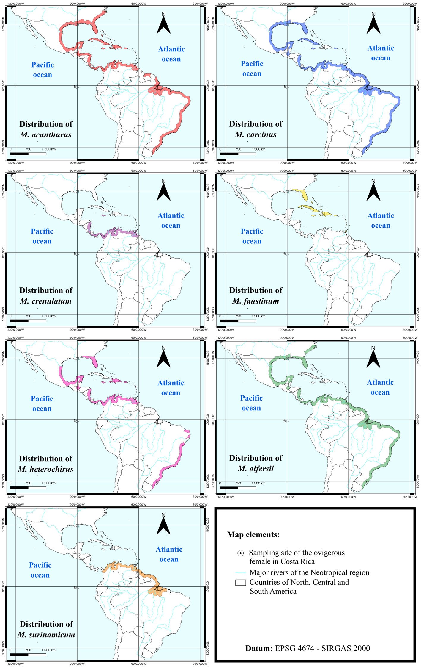
First maxilliped (Fig. 3E): biramous; coxa without setae; basis with 4 short simple setae arranged 1 + 2 + 1; endopod unarticled with 3 terminal simple setae, 1 short and 2 long; exopod unarticled, with 4 long terminal plumose natatory setae; endopod approximately 3 times shorter than exopod. Second maxilliped (Fig. 3F): biramous; coxa without setae; basis with 1 short simple seta; endopod 3-articled, first with 0, second with 1 terminal plumose, and third with 5, 1 short proximal simple, 3 short terminal simple and 1 short terminal sparsely plumose setae, respectively; exopod unarticled with 4 long terminal plumose natatory setae; endopod slightly shorter than exopod.
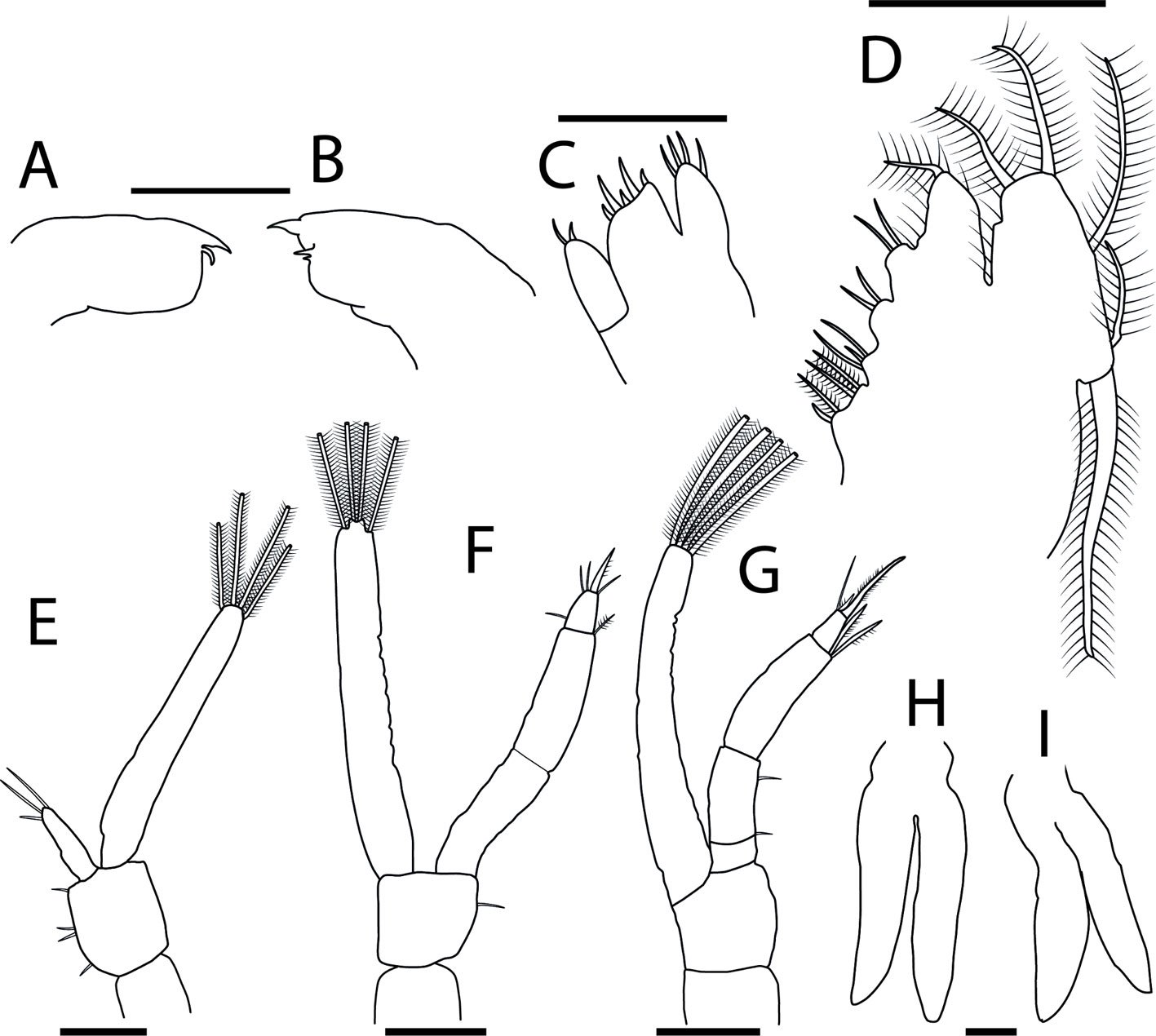
Third maxilliped (Fig. 3G): biramous; coxa and basis without setae; endopod 4-articled, first article without setae, second with 1 short proximal simple, and 1 short subterminal simple, third with 2 long terminal plumose, and fourth with 3 terminal setae, 1 long simple, 1 short plumose and 1 long plumose; exopod unarticled with 4 long terminal plumose natatory setae; endopod and exopod of similar length. Pereiopods (Fig. 3H, I): first and second rudimentary and biramous, second slightly longer than the first; third, fourth and fifth absent. Telson (Fig. 2E): posterior bilobed region broader than the anterior, with 7 + 7 plumose setae, outer 2 plumose only in inner margin; minute spinules along the posterior margin and around the bases of 3 + 3 inner setae.
Remarks
The morphological description of Zoea I of Macrobrachium crenulatum enables the comparison among the first zoeae of closely related congeners as well as the definition of some morphological characteristics. All the species included in the comparison exhibit type I development, characterized by an extended larval development and an amphidromous life cycle (Bauer, 2013). This contrasts with type II development, which involves a partially abbreviated larval development and is common in freshwater species, and type III development, which is marked by a completely abbreviated larval development and is typical of species inhabiting mountain streams (Jalihal et al., 1993; Pileggi et al., 2014; Vieira et al., 2017). Adults of amphidromous species typically inhabit both freshwater and brackish environments, except for M. crenulatum, M. faustinum, and M. heterochirus, whose adults have been reported exclusively in freshwater (Holthuis, 1950; Hunte, 1980; Vega-Perez, 1984; Vieira et al., 2017).
Before comparing the morphology of the Zoea I among species, it is important to consider that most of the larval descriptions included in Table 1 were published at different times, each reflecting the research context on decapod larval morphology of that period. Thus, many of the current consensuses on terminology (e.g., Clark et al., 1998) postdate some of the descriptions examined. Moreover, recent studies employ more advanced technologies than those available in the 1970s, 80s and 90s, enabling, for example, more accurate and detailed descriptions of setal types and number of articles. Therefore, some inconsistencies were detected during the comparisons of the published descriptions. Thus, we aimed to distinguish true morphological differences of the larvae from inconsistencies likely resulting from the limited technological capabilities used in earlier studies. Although we kept the original terminology used by the authors in our table, in the following comparison we focus on taxonomic informative differences, highlighting instances where a variation may result from misinterpretation.
Macrobrachium crenulatum and M. olfersii have been considered part of the same species complex due to the high morphological similarity of adults (Rossi & Mantelatto, 2013; Villalobos-Figueroa, 1967). Their close phylogenetic relationship was later confirmed using molecular data by Pileggi et al. (2014) and, more recently, by Pantaleão et al. (2025). For M. olfersii, 2 larval descriptions of first zoea are available. Dugger and Dobkin (1975) provided the first, describing Zoea I of this species from females collected in Florida (USA). Later, Melo and Brossi-Garcia (2005) provided a description for hatched larvae of Macrobrachium birai Lobão, Melo & Fernandes, 1986, obtained from a female collected in São Paulo (Brazil). Subsequently, however, M. birai was regarded as a junior synonymous of M. olfersii by Pileggi and Mantelatto (2012). Thus, both studies are treated here as descriptions of the first zoeal stage of M. olfersii. Although generally similar, both descriptions show some differences in the number of cuticular outgrowths on the antennal flagellum, maxilla coxal endite, and maxilliped endopods. Considering that each study worked with larvae from distinct latitudes (USA and Brazil) with different temperature regimes and oceanographic dynamics, these differences may reflect plasticity in larval morphology, a phenomenon that has partially explored in the scientific literature (Sandifer & Smith, 1979; Thatje & Bacardit, 2000; Wehrtmann & Albornoz, 2003). For the comparison between M. crenulatum and M. olfersii, we focused only on features that are consistent across both descriptions of M. olfersii, avoiding traits that showed intraspecific variation. In Table 1, when differences are observed in the description of Zoea I of M. olfersii, data from both descriptions are presented (Dugger & Dobkin, 1975; Melo & Brossi-Garcia, 2005).
The maxillipeds are considerably distinct between M. crenulatum and M. olfersii. They differ by the number of plumose setae on the third maxilliped exopod: Macrobrachium crenulatum presents only 4 terminal plumose setae, while the first zoea of M. olfersii has 2 subterminal plumose setae in addition to the 4 terminal ones. Moreover, the basis of the first maxilliped bears one simple seta in M. olfersii, but 4 (1 + 2 + 1) in M. crenulatum. Finally, it is important to mention that the larval description published by Dugger and Dobkin (1975) reports a difference in the number of articles on the exopod of maxillipeds: 2 in M. olfersii versus only one in M. crenulatum. However, aside from being absent in the description from Melo and Brossi-Garcia (2005), this apparent difference may result from a misinterpretation of the number of articles in maxilliped exopods of M. olfersii, since the presence of only 1 article appears to be a consistent pattern among American species of Macrobrachium, regardless of whether they exhibit type I development (e.g., M. carcinus, M. heterochirus and M. surinamicum) or type II (e.g., Macrobrachium iheringi [Ortmann, 1897] and Macrobrachium jelskii [Miers, 1877]) (Bueno & Rodrigues, 1995; Choudhury, 1970, 1971; Magalhães, 2000; Pantaleão et al., 2025; Vega-Perez, 1984; Vieira et al., 2017).
Several morphological features can be used to distinguish the first zoeae of M. crenulatum and M. carcinus, 2 species whose geographic distributions partially overlap. Notably, these 2 species differ in the pattern of setae present on the endopod of the third maxilliped: M. crenulatum has setae on all 4 articles of the third maxilliped endopod (1, 1, 2, 1 + 2), while Zoea I of M. carcinus presents setae only on the last article (0, 0, 0, 1 + 2 or 3) (Choudhury, 1971). Analysis of the larval description of M. carcinus reveals possible inconsistencies in terminology. In several instances, the term “spine” is used to refer to a “seta” and vice-versa. Additionally, although illustrated, the second maxilliped of the first zoea of M. carcinus was not formally described, being mentioned only briefly within the description of the third maxilliped. These inconsistencies hinder a comprehensive morphological comparison and complicate phylogenetic inferences based on larval characters. Therefore, given the aforementioned issues related to technological advances and terminology standardization, we strongly recommend a redescription of the first zoeal stage of M. carcinus.
Macrobrachium heterochirus is a species closely related to M. crenulatum both geographically and phylogenetically (Pantaleão et al., 2025; Pileggi et al., 2014), and the adults are morphologically distinct enough to be readily distinguished. Zoea I of both species, in turn, differ on the setal pattern of maxilla, both in the number and type of setae on coxal and basial endites: Macrobrachium crenulatum has 4 setae, one simple and 3 plumose, on the coxal endite and 5 simple setae on the basial endite, whereas the first zoea of M. heterochirus bears 5 setae, 4 plumose and one simple, on the coxal endite, and the basial endite carries only 4 plumose setae. According to the descriptions, these species also differ in the number of aesthetascs on the antennule exopod: 4 in M. crenulatum, and 3 in M. heterochirus (Vega-Perez, 1984). However, this difference may reflect a misinterpretation. Possibly, the simple seta described by the author as part of antennule exopod of M. heterochirus could in fact be an aesthetasc, bringing the total to 4, as observed in other species such as M. crenulatum and M. olfersii. Similar misunderstandings regarding the number of aesthetascs of the antennule may also applied to the descriptions of M. acanthurus, M. carcinus, M. faustinum, and M. surinamicum.
Several morphological characteristics allow the distinction between Zoea I of M. crenulatum and M. acanthurus, both species occurring in Costa Rica (Fig. 1). One of the most conspicuous features for identification is the number of aesthetascs on the antennule (4 on the first and only 3 on the latter), although this difference may reflect a misinterpretation in the earliest description, which dates back 56 years (Choudhury, 1970). Additionally, M. crenulatum has a spine on the protopod of the antenna, which is absent in M. acanthurus. Another notable difference lies in the number of endopod articles of the second maxilliped: Macrobrachium crenulatum has 3, whereas M. acanthurus presents 4, and the setal pattern on this structure also differs (Table 1). Finally, the telson of M. crenulatum bears small spines between the 3 innermost plumose setae, while in M. acanthurus, spines are present between all the setae of the telson.
As with M. acanthurus, several traits can be used to distinguish Zoea I of M. crenulatum and M. faustinum (Table 1), species that are relatively close phylogenetically (Pantaleão et al., 2025). Notably, the number of aesthetascs present in the antennule differs, with M. crenulatum having 4 and M. faustinum only 3. As previously noted, this feature should be interpreted cautiously, as the older description may not be fully accurate in this regard. Additionally, the scaphocerite of M. faustinum lacks a spine present in the first larval stage of M. crenulatum, and the molar process of the right mandible in M. crenulatum is unarmed, whereas in M. faustinum it bears 2 protuberances (Hunte, 1980).
Finally, several larval characteristics can also be used to identify the first zoeae of M. crenulatum and M. surinamicum, species relatively closely related according to Pantaleão et al. (2025). The differences between the newly hatched larvae refer to the number of articles on the scaphocerite (5 in M. crenulatum and 6 in M. surinamicum), the number of spines on basial endite of maxillule (5 in M. crenulatum and 2 in M. surinamicum), and the position of setulae on the outer pair of setae of telson margin. In M. crenulatum, setulae occur only on inner margin of the outer pair of setae of the distal margin of the telson, whereas in M. surinamicum, they are present on both the inner and outer margins (Table 1). Interestingly, none of the other species with described Zoea I included in Table 1 have setulae on the outer margin of this pair of setae. Therefore, the phylogenetic significance of this trait warrants to be analyzed in future studies.
The present study represents a first step toward improving our knowledge of larval morphology of M. crenulatum. Although it focuses only on the first larval stage of a single brood of Macrobrachium species, the results contribute to a broader effort of providing larval descriptions for Neotropical species of the genus. This information offers valuable insights for both theoretical studies about the evolution of the morphology of Macrobrachium and practical applications in larval ecology and aquaculture research focused on larval development. Additionally, the investigation of the larval morphology of M. crenulatum helps to fill a gap in the larval descriptions of a lineage of species of Macrobrachium for which no larval data were previously available (Pantaleão et al., 2025). This line of research should be continued by describing the larvae of other species phylogenetically close to M. crenulatum, such as M. digueti and M. hancocki, to broaden our understanding of phylogenetic relationships among these freshwater shrimps. Finally, our results highlight the need for redescriptions of the first zoea of several species of Macrobrachium, aimed at updating the larval terminology and clarifying ambiguous characters, which would in turn facilitate morphological comparisons and phylogenetic analysis.
Identification key for the compared species of Macrobrachium with ELD from Neotropics based on morphological traits of Zoea I
1. First article of third maxilliped endopod with setae 2
1’. First article of third maxilliped endopod without setae 3
2. Scaphocerite with 5 articles; basial endite of maxillule with 5 spines; most lateral pair of setae of telson margin with setulae only on inner margin M. crenulatum
2’. Scaphocerite with 6 articles; basial endite of maxillule with 2 spines; most lateral pair of setae of telson margin with setulae both on inner and outer margins M. surinamicum
3. Basial endite of first maxilliped with more than 1 seta; endopod of third maxilliped with 4 articles 4
3’. Basial endite of first maxilliped with only 1 seta; endopod of third maxilliped with 3 articles M. olfersii
4. Scaphocerite with 10 plumose setae; first maxilliped endopod with 3 cuticular outgrowths 5
4’. Scaphocerite with 11 plumose setae; first maxilliped endopod with 4 cuticular outgrowths M. heterochirus
5. Scaphocerite with 12 cuticular outgrowths; maxilla coxal endite with 4 plumose setae 6
5’. Scaphocerite with 11 cuticular outgrowths; maxilla coxal endite with 3 plumose setae M. faustinum
6. Lobes of maxilla basial endite with 2 plumose setae each M. acanthurus
6’. Lobes of maxilla basial endite with 2 plumose setae and 1 simple seta each M. carcinus
Acknowledgements
This study is result of the course “Special Topics in Comparative Biology: Larval morphology and phylogenetic relationships in decapod crustaceans” under the responsibility of FLM and JAFP and as part of Postgraduate Program in Comparative Biology at Faculty of Philosophy, Sciences and Letters at Ribeirão Preto. The authors are grateful to the LBSC team, in special to Gabriel L. Bochini, who helped with some dissections and slide preparation. We acknowledge the financial support provided by Fundação de Amparo à Pesquisa do Estado de São Paulo (FAPESP) (Projetos Temáticos BIOTA Proc. 2010/50188-8 and INTERCRUSTA Proc. 2018/13685-5) and Conselho Nacional de Desenvolvimento Científico e Tecnológico (CNPq) (PPBio 07/2023 – Linha 8: Rede Costeira Marinha Proc. 442421/2023-0). FLM and ISW are thankful for the financial contribution supplied by CNPq (Proc. 491490/2004-6, 490353/2007-0, 490314/2011-2; 471011/2011-8) and CONICIT – Costa Rica (CII- 001-08, IQ-0001-11) during the development of the International Cooperative Project, which was crucial for the collection of the female with embryos and collaboration in the Brazil-Costa Rica research program. FLM thanks CNPq for an ongoing research grant (PQ 302706/2025-9). LOR and RP thank PhD grants provided by Coordenação de Aperfeiçoamento de Pessoal de Nível Superior (CAPES) (PROEX – Proc. 88887.804708/2023-00 and 88887.896987/2023-00, respectively). RP and LOR also thank the ongoing PhD fellowships by FAPESP (Proc. 2024/15232-9 and 2025/01018-8, respectively). The ovigerous female was collected under the collection and genetic access permit (Resolución No. 377 – Comisión Institucional de Biodiversidad de la Universidad de Costa Rica) to ISW. We also thank the anonymous reviewers and associate editor for their valuable comments, which improved the quality of the manuscript.
References
Almeida, A. O., Alves-Coelho, P., Rocha-Luz, J., Almeida-dos Santos, J. T., & Ribeiro-Ferraz, N. (2008). Decapod crustaceans in fresh waters of southeastern Bahia, Brazil. Revista de Biología Tropical, 56, 1225–1254. https://doi.org/10.15517/rbt.v56i3.5706
Anger, K. (2001). The biology of decapod crustacean larvae. Lisse, South Holland: AA Balkema Publishers.
Anger, K. (2013). Neotropical Macrobrachium (Caridea: Palaemonidae): on the biology, origin, and radiation of freshwater-invading shrimp. Journal of Crustacean Biology, 33, 151–183. https://doi.org/10.1163/1937240X-00002124
Bauer, R. T. (2011a). Amphidromy and migrations of freshwater shrimps. I. Costs, benefits, evolutionary origins, and an unusual case of amphidromy. New Frontiers in Crustacean Biology, 15, 145–156. https://doi.org/10.1163/ej.9789004174252.i-354.108
Bauer, R. T. (2011b). Amphidromy and migrations of freshwater shrimps. II. Delivery of hatching larvae to the sea, return juvenile upstream migration, and human impacts. New Frontiers in Crustacean Biology, 15, 157–168. https://doi.org/10.1163/EJ.9789004174252.I-354.115
Bauer, R. T. (2013). Amphidromy in shrimps: a life cycle between rivers and the sea. Latin American Journal of Aquatic Research, 41, 633–650. https://doi.org/10.3856/vol41-issue4-fulltext-2
Bouvier, E. L., (1895). Sur les palémons receuillis dans les eaux douces de la Basse-Californie par M. Diguet. Bulletin du Muséum d’Histoire Naturelle, 1, 159–162.
Bowles, D. E., Aziz, K., & Knight, C. L. (2000). Macrobrachium (Decapoda: Caridea: Palaemonidae) in the contiguous United States: a review of the species and an assessment of threats to their survival. Journal of Crustacean Biology, 20, 158–171. https://doi.org/10.1163/20021975-99990025
Bueno, S. L. S., & Rodrigues, S. A. (1995). Abbreviated larval development of the freshwater prawn, Macrobrachium iheringi (Ortmann, 1897) (Decapoda, Palaemonidae), reared in the laboratory. Crustaceana, 68, 665–686. https://doi.org/10.1163/156854095X01880
Burkenroad, M. D. (1963). The evolution of the Eucarida (Crustacea, Eumalacostraca), in relation to the fossil record. Tulane Studies in Geology, 2, 3–17.
Clark, P. F., Calazans, D. K., & Pohle, G. W. (1998). Accuracy and standardization of brachyuran larval descriptions. Invertebrate Reproduction & Development, 33, 127–144. https://doi.org/10.1080/07924259.1998.9652627
Clark, P. F., & Cuesta, J. A. (2015). Larval systematics of Brachyura. In P. Castro, P. J. F. Davie, D. Guinot, F. R. Schram, & J. C. von Vaupel-Klein (Eds.), Treatise on Zoology-Anatomy, Taxonomy, Biology. The Crustacea 9C (pp. 981–1048). Leiden, South Holland: Brill. https://doi.org/10.1163/9789004190832_020
Chace, F. A., & Bruce, A. J. (1993). The caridean shrimps (Crustacea: Decapoda) of the Albatross Philippine expedition 1907-1910, part 6: superfamily Palaemonoidea. Smithsonian Contributions to Zoology, 543, 1–152. https://doi.org/10.5479/si.00810282.543
Choudhury, P. C. (1970). Complete larval development of the palaemonid shrimp Macrobrachium acanthurus (Wiegmann, 1836), reared in the laboratory. Crustaceana, 18, 113–132. https://doi.org/10.1163/156854070X00743
Choudhury, P. C. (1971). Complete larval development of the palaemonid shrimp Macrobrachium carcinus (L.), reared in the laboratory (Decapoda, Palaemonidae). Crustaceana, 20, 51–69. https://doi.org/10.1163/156854071X00526
De Grave, S., & Fransen, C. H. J. M. (2011). Carideorum catalogus: the recent species of the dendrobranchiate, stenopodidean, procarididean and caridean shrimps (Crustacea: Decapoda). Zoologische Mededelingen, 85, 195–589.
de Saussure, H. (1857). Diagnoses de quelques Crustacés nouveaux de l’Amérique tropicale. Revue et Magasin de Zoologie, Ser. 2, 9, 501–505.
Dugger, D. M., & Dobkin, S. (1975). A contribution to knowledge of the larval development of Macrobrachium olfersii (Wiegmann, 1836) (Decapoda, Palaemonidae). Crustaceana, 29, 1–30. https://doi.org/10.1163/156854075×00018
Ferreira, R. S., Vieira, R. R. R., & D’Incao, F. (2010). The marine and estuarine shrimps of the Palaemoninae (Crustacea: Decapoda: Caridea) from Brazil. Zootaxa, 2606, 1–24. https://doi.org/10.11646/zootaxa.2606.1.1
Fujita, Y., Davie, P. J., & Ng, P. K. (2015). A new stygobitic prawn of the genus Macrobrachium Spence Bate, 1864, from anchialine caves in Christmas Island, Indian Ocean; with a rediagnosis of M. miyakoense Komai & Fujita, 2005 (Crustacea: Decapoda: Caridea: Palaemonidae). Raffles Bulletin of Zoology, 63, 610–625.
Garm, A. (2004). Revising the definition of the crustacean seta and setal classification systems based on examination of the mouthpart setae of seven species of decapods. Zoological Journal of the Linnean Society, 142, 233–252. https://doi.org/10.1111/j.1096-3642.2004.00132.x
Holthuis, L. B. (1948). Note on some Crustacea Decapod Natantia from Surinam. Proceedings van de Koninklijke Nederlandsche Akademie van Wetenschappen, 51, 1104–1113.
Holthuis, L. B. (1950). Preliminary descriptions of twelve new species of palaemonid prawns from American waters (Crustacea Decapoda). Proceedings van de Koninklijke Nederlandsche Akademie van Wetenschappen, 53, 93–99.
Holthuis, L. B. (1952). A general revision of the Palaemonidae (Crustacea, Decapoda, Natantia) of the Americas. II. The subfamily Palaemonidae. Occasional Papers of the Allan Hancock Foundation, 12, 1–396.
Hunte, W. (1979). The rediscovery of the freshwater shrimp Macrobrachium crenulatum in Jamaica. Studies on the Fauna of Curaçao and other Caribbean Islands, 58, 69–74.
Hunte, W. (1980). The larval development of the shrimp Macrobrachium faustinum reared at the laboratory. Caribbean Journal of Science, 15, 49–68.
Jalihal, D. R., Sankolli, K. N., & Shenoy, S. (1993). Evolution of larval developmental patterns and the process of freshwaterization in the prawn genus Macrobrachium Bate, 1868 (Decapoda, Palaemonidae). Crustaceana, 65, 365–376. https://doi.org/10.1163/156854093X00793
Lai, J. C. Y., Thoma, B. P., Clark, P. F., Felder, D. L., & Ng, P. K. L. (2013). Phylogeny of eriphioid crabs (Brachyura, Eriphioidea) inferred from molecular and morphological studies. Zoologica Scripta, 43, 52–64. https://doi.org/10.1111/zsc.12030
Lara, R., & Wehrtmann, I. S. (2011). Diversity, abundance and distribution of river shrimps (Decapoda: Caridea) in the largest river basin of Costa Rica, Central America. In A. Asakura & C. Fransen (Eds.), New Frontiers in Crustacean Biology (pp. 197–211). Leiden, South Holland: Brill. http://dx.doi.org/10.1163/ej.9789004174252.i-354.140
Latreille, P. A. (1802). Histoire naturelle, générale et particulière des crustacés et des insectes. Familles naturelles des genre. Ouvrage faisant suite à l‘Histoire Naturelle générale et particulière, composée par Leclerc de Buffon, et rédigée par C.S. Sonnini, membre de plusieurs Sociétés savantes. de L‘imprimerie de F. Dufart, Paris.
Liu, M. Y., Cai, Y. X., & Tzeng, C. S. (2007). Molecular systematics of the freshwater prawn genus Macrobrachium Bate, 1868 (Crustacea: Decapoda: Palaemonidae) inferred from mtDNA sequences, with emphasis on East Asian species. Zoological Studies, 46, 272–289.
Lobão, V. L., Melo, G. A. S., & Fernandes, W. (1986). Descrição de uma nova espécie do gênero Macrobrachium (Crustacea: Decapoda: Palaemonidae) da região sul de São Paulo. In Resumos do Congresso Brasileiro de Zoologia, Volume 13. Cuiabá.
Magalhães, C. (2000). Abbreviated larval development of Macrobrachium jelskii (Miers, 1877) (Crustacea: Decapoda, Palaemonidae) from the Rio Solimões floodplain, Brazil, reared in the laboratory. Nauplius, 8, 1–14.
Magalhães, C., & Pereira, G. (2007). Assessment of the decapod crustacean diversity in the Guayana Shield region aiming at conservation decisions. Biota Neotropica, 7, 111–124. https://doi.org/10.1590/s1676-06032007000200013
Melo, S. G., & Brossi-Garcia, A. L. (2005). Desenvolvimento larval de Macrobrachium birai Lobão, Melo & Fernandes (Crustacea, Decapoda, Caridea, Palaemonidae) em laboratório. Revista Brasileira de Zoologia, 22, 131–152. https://doi.org/10.1590/S0101-81752005000100016
Miers, E. J. (1877). On a collection of Crustacea, Decapoda and Isopoda, chiefly from South America, with descriptions of new genera and species. Proceedings of the Zoological Society of London, 43, 653–679.
Murienne, J., Chevalier, J., & Clavier, S. (2022). On the presence of the giant freshwater prawn, Macrobrachium rosenbergii, in French Guiana confirmed by citizen science and genetic analyses. Water Biology and Security, 1, 100039. https://doi.org/10.1016/j.watbs.2022.100039
Murphy, N. P., & Austin, C. M. (2005). Phylogenetic relationships of the globally distributed freshwater prawn genus Macrobrachium (Crustacea: Decapoda: Palaemonidae): biogeography, taxonomy and the convergent evolution of abbreviated larval development. Zoologica Scripta, 34, 187–197. https://doi.org/10.1111/j.1463-6409.2005.00185.x
Ortmann, A. (1897). Os camarões da agua doce da America do Sul. Revista do Museu Paulista, 2, 173–216.
Pantaleão, J. A. F., Gregati, R. A., Taddei, F. G., & Costa, R. C. (2011). Morphology of the first larval stage of Macrobrachium brasiliense (Heller, 1868) (Caridea: Palaemonidae). Nauplius, 19, 79–85. https://doi.org/10.1590/S0104-64972011000100009
Pantaleão, J. A. F., Mantelatto, F. L., & Costa, R. C. (2021). The first larval stage (Zoea I) description of the caridean shrimp Ogyrides occidentalis (Ortmann, 1893) (Alpheoidea: Ogyrididae) reveals congruence with taxonomic status. Biota Neotropica, 21, e20201118. https://doi.org/10.1590/1676-0611-BN-2020-1118
Pantaleão, J. A. F., Peres, P. A., & Mantelatto, F. L. (2025). Mapping the congruence between larval morphology and molecular phylogeny: Convergent adaptations of fresh-
water shrimps (Decapoda, Caridea). Zoologica Scripta, 54, 376–393. https://doi.org/10.1111/zsc.12709
Pileggi, L. G., & Mantelatto, F. L. (2010). Molecular phylogeny of the freshwater prawn genus Macrobrachium (Decapoda, Palaemonidae), with emphasis on the relationships among selected American species. Invertebrate Systematics, 24, 194–208. https://doi.org/10.1071/IS09043
Pileggi L. G., & Mantelatto, F. L. (2012). Taxonomic revision of doubtful Brazilian freshwater shrimp species of genus Macrobrachium (Decapoda, Palaemonidae). Iheringia, Série Zoologia, 102, 426–437. https://doi.org/10.1590/S0073-47212012005000012
Pileggi, L. G., Rossi, N., Wehrtmann, I. S., & Mantelatto, F. L. (2014). Molecular perspective on the American transisthmian species of Macrobrachium (Caridea, Palaemonidae). Zookeys, 457, 109–131. https://doi.org/10.3897/zookeys.457.6818
Pohle, G. W., & Telford, M. (1981). Morphology and classification of decapod crustacean larval cerdae: a scanning electron microscope study of Dissodactylus crinitichelis Moreira, 1901 (Brachyura: Pinnotheridae). Bulletin of Marine Science, 31, 736–752.
Pompeu, P. D. S., Vieira, F., & Martinez, C. B. (2006). Utilização do mecanismo de transposição de peixes da Usina Hidrelétrica Santa Clara por camarões (Palaemonidae), bacia do rio Mucuri, Minas Gerais, Brasil. Revista Brasileira de Zoologia, 23, 293–297. https://doi.org/10.1590/s0101-81752006000100024
Poore, G. C., & Ahyong, S. T. (2023). Marine decapod Crustacea: a guide to families and genera of the world. Clayton, Victoria: CSIRO Publishing. https://doi.org/10.1071/9781486311798
Rafinesque, C. S. (1815). Analyse de la nature ou Tableau de l’univers et des corps organisés. Palermo: Published by the author.
Rossi, N. (2012). Revisão das espécies de Macrobrachium Bate, 1868, pertencentes ao complexo M. olfersii (Crustacea, Palaemonidae): análises morfológicas e moleculares (M.Sc. Thesis). Universidade de São Paulo. Brazil, São Paulo.
Rossi, N., & Mantelatto, F. L. (2013). Molecular analysis of the freshwater prawn Macrobrachium olfersii (Decapoda, Palaemonidae) supports the existence of a single species throughout its distribution. Plos One, 8, e54698. https://doi.org/10.1371/journal.pone.0054698
Sandifer, P. A., & Smith, T. I. (1979). Possible significance of variation in the larval development of palaemonid shrimp. Journal of Experimental Marine Biology and Ecology, 39, 55–64. https://doi.org/10.1016/0022-0981(79)90004-2
Sastry, A. N. (1983). Ecological aspects of reproduction. In F. J. Vernberg, & W. B. Vernberg (Eds.), The biology of Crustacea: environmental adaptations, Volume 8 (pp. 179–270). New York: Academic Press.
Shokita, S. (1985). Larval development of the palaemonid prawn, Macrobrachium grandimanus (Randall), reared in the laboratory, with special reference to larval dispersal. Zoological Science, 2, 785–803.
Spence Bate, C. (1868). On a new genus, with four new species, of freshwater prawns. Proceedings of the Zoological Society of London, 363–368.
Tejeda-Mazariegos, J. C., Ortiz, L. M. M., López-Mejía, M., Crandall, K. A., Pérez-Losada, M., & Frausto-Martínez, O. (2018). Freshwater crustacean decapods: an important resource of Guatemala. In S. Ray (Ed.), Biological resources of water (pp. 169–180). London: IntechOpen. https://doi.org/10.5772/intechopen.73638
Thatje, S., & Bacardit, R. (2000). Morphological variability in larval stages of Nauticaris magellanica (A. Milne Edwards, 1891) (Decapoda: Caridea: Hippolytidae) from South American waters. Bulletin of Marine Science, 66, 375–398.
Valencia, D. M., & Campos, M. R. (2007). Freshwater prawns of the genus Macrobrachium Bate, 1868 (Crustacea: Decapoda: Palaemonidae) of Colombia. Zootaxa, 1456, 1–44. https://doi.org/10.11646/zootaxa.1456.1.1
Vega-Perez, L. A. (1984). Desenvolvimento larval de Macrobrachium heterochirus (Wiegmann, 1836), Macrobrachium amazonicum (Heller, 1862) e Macrobrachium brasiliense (Heller, 1868) (Crustacea, Decapoda, Palaemonidae), em laboratório (Ph.D. Thesis). Universidade de São Paulo. Brazil, São Paulo.
Vieira, R. R. R., Santos, C. R. M., & Anker, A. (2017). Morphology of the first zoeal stage of Macrobrachium surinamicum Holthuis, 1948 (Malacostraca, Decapoda, Palaemonidae) hatched in the laboratory. Crustaceana, 90, 1337–1350. https://doi.org/10.1163/15685403-00003723
Villalobos-Figueroa, A. (1967). Problemas de especiación en América de un grupo de Palaemonidae del género Macrobrachium. FAO Fisheries Report, 57, 1055–1066.
Villalobos-Hiriart, J. L., & Nates-Rodríguez, J. C. (1990). Dos especies nuevas de camarones de agua dulce del género Macrobrachium Bate, (Crustacea, Decapoda, Palaemonidae), de la vertiente occidental de México. Anales del Instituto de Biología, Universidad Nacional Autónoma de México, Serie Zoología, 61, 1–11.
Wehrtmann, I. S., & Albornoz, L. (2003). Larvae of Nauticaris magellanica (Decapoda: Caridea: Hippolytidae) reared in the laboratory differ morphologically from those in nature. Journal of the Marine Biological Association of the United Kingdom, 83, 949–957. https://doi.org/10.1017/S0025315403008130h
Wiegmann, A. (1836). Beschreibung einiger neuen Crustaceen des Berliner Museums aus Mexiko und Brasilien. Archiv für Naturgeschichte, 2, 145–151.
Wowor, D., Muthu, V., Meier, R., Balke, M., Cai, Y., & Ng, P. K. L. (2009). Evolution of life history traits in Asian freshwater prawns of the genus Macrobrachium (Crustacea: Decapoda: Palaemonidae) based on multilocus molecular phylogenetic analysis. Molecular Phylogenetics and Evolution, 52, 340–350. https://doi.org/10.1016/j.ympev.2009.01.002

Cuatro registros nuevos del género Septoglomus (Glomeromycota) en México
Four new records of the genus Septoglomus (Glomeromycota) in Mexico
Reyna P. Hipólito-Piedras a, Heriberto Méndez-Cortés b, *, Hugo M. Ramírez-Tobias b, Victor Olalde-Portugal c, Carlos Arturo Aguirre-Salado d, Ángel Natanael Rojas-Velázquez b y Aracely Mena-Echevarríae
a Universidad Autónoma de San Luis Potosí, Facultad de Agronomía y Veterinaria, Doctorado en Ciencias Agropecuarias, Carretera San Luis Potosí-Matehuala Km. 14.5, Ejido Palma de la Cruz, 78321 Soledad de Graciano Sánchez, San Luis Potosí, México
b Universidad Autónoma de San Luis Potosí, Facultad de Agronomía y Veterinaria, Carretera San Luis Potosí- Matehuala Km. 14.5, Ejido Palma de la Cruz, 78321 Soledad de Graciano Sánchez, San Luis Potosí, México
c Instituto Politécnico Nacional, Centro de Investigación y de Estudios Avanzados-Unidad Irapuato, Departamento de Biotecnología y Bioquímica, Libramiento Norte Carretera Irapuato-León Km 9.6, 36824 Irapuato, Guanajuato, México
d Universidad Autónoma de San Luis Potosí, Facultad de Ingeniería, Av. Dr. Manuel Nava 4, 78290 San Luis Potosí, San Luis Potosí, México
e Instituto Nacional de Investigaciones Forestales Agrícolas y Pecuarias, Campo Experimental General Terán-INIFAP, Km 31 Carretera Montemorelos-China, 67400 General Terán, Nuevo León, México
*Autor para correspondencia: heriberto.mendez@uaslp.mx (H. Méndez-Cortés)
Recibido: 13 febrero 2024; aceptado: 23 julio 2025
Resumen
Los hongos micorrizógenos arbusculares (HMA) son organismos esenciales y de suma importancia para las plantas terrestres. Se seleccionaron distintas comunidades vegetales de México en los estados de Coahuila, Guanajuato, San Luis Potosí, Tamaulipas y Veracruz, en donde se recolectó suelo rizosférico con el objetivo de aislar esporas de HMA. La identificación taxonómica se llevó a cabo mediante el análisis de las características morfológicas de las esporas, comparándolas con los artículos originales de cada especie descrita. Se identificaron 4 especies de HMA pertenecientes al género Septoglomus (S. altomontanum, S. fuscum, S. furcatum y S. turnauae), que constituyen su primer registro en México. Con estas 4 especies, la riqueza total de HMA en México se eleva a 171, lo cual evidencia una diversidad significativa de HMA en las comunidades vegetales del país.
Palabras clave: Glomeromycota; Micorriza arbuscular; Glomeraceae
Abstract
Arbuscular mycorrhizal fungi (AMF) are essential and extremely important organisms for terrestrial plants. Different plant communities of Mexico were selected in the states of Coahuila, Guanajuato, San Luis Potosí, Tamaulipas and Veracruz, where rhizospheric soil was collected with the objective of isolating AMF spores. Taxonomic identification was carried out by analyzing the morphological characteristics of the spores, comparing them with the original articles of each described species. Four species of AMF belonging to the genus Septoglomus (S. altomontanum, S. fuscum, S. furcatum, and S. turnauae) were identified, constituting their first record in Mexico. With the record of these 4 species, the total richness of AMF in Mexico rises to 171, evidencing a significant diversity of AMF in the plant communities of the country.
Keywords: Glomeromycota; Arbuscular mycorrhizae; Glomeraceae
Introducción
Los hongos micorrizógenos arbusculares (HMA) son organismos cruciales y de suma importancia en la ecología y fisiología de las plantas terrestres. Fueron considerados inicialmente en el filo Zygomycota; sin embargo, a través de sus características moleculares, morfológicas y ecológicas, fueron reorganizados en un nuevo filo monofilético denominado Glomeromycota (Schüßler et al., 2001). Actualmente, la clasificación taxonómica de los HMA incluye 3 clases, 4 órdenes y 43 géneros (Schüβler, 2025; Wijayawardene et al., 2020).
Uno de los géneros incluidos en Glomeromycota es Septoglomus. Originalmente, las especies que ahora se ubican en este género se agruparon dentro del género Glomus. Sin embargo, Schüßler y Walker (2010) las reubicaron en el género Funneliformis, basándose en criterios morfológicos. Posteriormente, Oehl et al. (2011) dividieron Glomus en 2 grupos taxonómicos, proponiendo los géneros Simiglomus y Septoglomus con base en análisis de secuencias ribosomales y en la morfología. Sin embargo, Redecker et al. (2013) validaron únicamente al género Septoglomus y recomendaron conservar su estatus en espera de mayor evidencia, particularmente a partir de estudios filogenéticos del DNAr.
La especie de referencia taxonómica para la clasificación del género Septoglomus fue Glomus constrictum (Trappe) Sieverd., GA Silva et Oehl (Glomeraceae) (actualmente, S. constrictum). A partir de ésta, se establecieron los criterios taxonómicos del género, que se caracterizan por la producción de esporas de manera individual o en pequeños grupos. Dichas esporas presentan una o múltiples capas y están conectadas a hifas que se extienden de forma continua hasta la pared de la espora, adoptan una forma cilíndrica o de embudo y presentan un poro cerrado por un septo ubicado en la base o debajo de la pared de la espora. Generalmente, estas esporas no reaccionan a la aplicación del reactivo de Melzer; sin embargo, sus estructuras adquieren una coloración azul oscuro al ser tratadas con azul de tripano (Oehl et al., 2011).
Actualmente, el género Septoglomus comprende 13 especies, lo que representa aproximadamente 4% de la diversidad total de HMA. Estas especies han sido documentadas en diversos estudios, como los de Błaszkowski et al. (2004, 2014, 2013, 2023), Goto et al. (2013), Symanczik et al. (2014), Chimal-Sánchez et al. (2020), Oehl et al. (2011, 2019), Palenzuela et al. (2013) y Guillén et al. (2020). Sin embargo, la clasificación de algunas de estas especies continúa en revisión. Por ejemplo, recientemente S. deserticola G.A. Silva, Oehl et Sieverd. y S. viscosum C. Walker, D. Redecker, D. Stille et A. Schüßler (Glomeraceae) fueron reclasificados en el nuevo género Blaszkowskia, con base en análisis filogenéticos y en su morfología distintiva (da Silva et al., 2023).
Las especies del género Septoglomus han sido registradas en diferentes continentes; en Europa, por Palenzuela et al. (2013), Blaszkowski et al. (2014), Oehl et al. (2019) y Guillén et al. (2020); en América, por Błaszkowski et al. (2013), Goto et al. (2013) y Chimal-Sánchez et al. (2020); en Asia, por Symanczik et al. (2014) y Oehl et al. (2019) y en África por Błaszkowski et al. (2010, 2013). El registro de estas especies fue en dunas marítimas, bosques lluviosos y tropicales, así como en matorrales xerófilos. No obstante, se ha observado que este género demuestra una destacada capacidad de adaptación y una dominancia notable en entornos áridos, en comparación con otros géneros de HMA. Además, muestra una eficiencia notable en la colonización de las raíces de cultivos agrícolas y forestales (Guardiola-Márquez et al., 2022).
En México se han identificado 4 especies del género Septoglomus. Sin embargo, es crucial llevar a cabo investigaciones a mayor escala, que abarquen tanto el ámbito ecológico como el morfológico para comprender mejor su distribución en el país. Asimismo, intensificar el muestreo para aumentar el conocimiento sobre la riqueza de especies de HMA en el territorio nacional (Polo-Marcial et al., 2021). El objetivo de esta investigación fue contribuir al conocimiento sobre la diversidad de Septoglomus mediante la documentación de 4 nuevos registros obtenidos en distintos tipos de vegetación de México.
Materiales y métodos
El muestreo del suelo rizosférico se realizó durante la época de lluvias (agosto, 2020-2021), en 6 sitios ubicados en 4 estados de la República Mexicana (fig. 1, tabla 1). En cada uno de los sitios se estableció un transecto de 1 km, donde cada 200 m se tomó una submuestra a una profundidad de 0 a 20 cm, la cual fue trasladada al laboratorio de Fitopatología, de la Facultad de Agronomía y Veterinaria, de la Universidad Autónoma de San Luis Potosí.
La extracción de esporas de HMA se realizó por el método de tamizado húmedo y decantación (Gerdemann y Nicolson, 1963), utilizando 500 g de suelo seco, seguido de una centrifugación en sacarosa al 70% a 2,000 rpm (Daniels y Skipper, 1982). Las esporas se montaron en preparaciones permanentes con alcohol polivinílico-lacto-glicerol (PVLG) y PVLG con reactivo de Melzer (INVAM, 2023).
La identificación se llevó a cabo de acuerdo con las características morfológicas de la espora, como lo sugieren da Silva et al. (2023). Así, se registraron el tamaño, las características de la pared de la espora y de la hifa de sostén, y la reacción al reactivo de Melzer. La observación de tales características fue en un microscopio óptico Zeiss Primo Star (Jena, Alemania) con iluminación fija Koehler.
Las mediciones de las características de las esporas de HMA se realizaron en fotografías tomadas con el software de microscopía ZEN blue (versión 3.4) (Jena, Alemania), con objetivos 40x y 100x. Tales características se contrastaron con lo descrito en las claves dicotómicas de Palenzuela et al. (2013) y Oehl et al. (2019); así como con los artículos de referencia (Blaszkowski et al., 2013, 2014; Palenzuela et al., 2013) y se elaboraron claves para la identificación de las especies. Los ejemplares de referencia fueron depositados en el herbario Isidro Palacios, perteneciente al Instituto de Investigación de Zonas Desérticas, de la Universidad Autónoma de San Luis Potosí (SLPM).
Descripciones
Se identificaron un total de 62 especies de HMA, en los 9 sitios de muestreo. De éstas, 21% pertenecen al género Acaulospora, 15% a Glomus, 11% a Septoglomus, 10% a Ambispora, 10% a Rhizophagus, 5% a Entrophospora, 5% a Funneliformis, 5% a Gigaspora, 5% a Scutellospora, 3% a Diversipora y 10% restante se distribuye en igual proporción entre los géneros Blazskowskia, Dominikia, Pacispora y Sieverdingia.
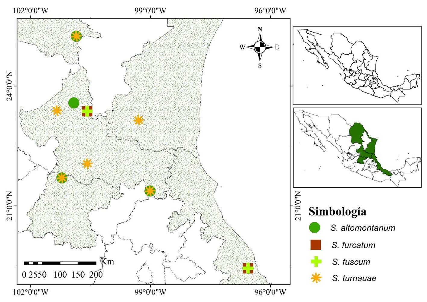
Figura 1. Distribución geográfica de sitios de muestreo y 4 especies del género Septoglomus en México.
Las especies registradas del género Septoglomus fueron: S. constrictum, S. mexicanum E. Chimal-Sánchez, C. Senés-Guerrero, NM Montaño, L. Varela, R. García-Sánchez, A. Pacheco, S. Montaño-Arias y SL Camargo-Ricalde, S. xanthium (Błaszk., Blanke, Renker y Buscot) GA Silva, Oehl y Sieverd., S. altomontanum Palenz., Oehl, Azcón-Aguilar y GA Silva, S. fuscum, S. furcatum Błaszk., Chwat, Kovács y Ryszka, y S. turnauae Błaszk., Chwat y Ryszka(Glomeraceae). Las últimas 4 son registro nacional, por lo cual se presenta la descripción morfológica y las ilustraciones correspondientes.
Tabla 1
Caracterización de los sitios de muestreo de Septoglomus en México.
| Estado | Sitio | Coordenadas geográficas (Datum WGS84) | Vegetación | Suelo | Clima |
| San Luis Potosí | 1. San José de Coronados | 23°34’35.4” N 100°55’09.5” O | Bosque de pino | Xerosol | Árido templado |
| 2. Xilitla | 21°22’21.4” N 99°00’39.0” O | Bosque mesófilo de montaña | Litosol | Semicálido húmedo | |
| 3. Matehuala | 23°21’51.1” N 100°35’01.7” O | Matorral xerófilo | Xerosol | Árido semicálido | |
| 4. Sierra de Álvarez | 22°03’06.3” N 100°34’50.8” O | Bosque de encino | Litosol | Semicálido | |
| 5. Charcas | 23°22’58.5” N 101°20’18.5” O | Pastizal | Xerosol | Semiárido | |
| Guanajuato | 6. San Felipe | 21°41’56.4” N 101°12’57.6” O | Bosque de encino | Feozem | Semiárido templado |
| Veracruz | 7. Plan de Higuera | 19°26’17.0” N 96°33’35.6” O | Bosque tropical caducifolio | Vertisol | Cálido subhúmedo |
| Coahuila | 8. Sierra Hermosa | 25°14’42” N 100°51’18” O | Bosque de pino | Litosol | Semiárido templado |
| Tamaulipas | 9. Jaumave | 23°08’26.0” N 99°17’48.4” O | Bosque de encino | Litosol | Semiárido templado |
Fuente: datos generados a partir de las capas disponibles en Geoportal y Enciclovida, México, Conabio (2018).
Septoglomus altomontanum Palenz., Oehl, Azcón-Aguilar y GA Silva, 2013.
Fig. 2a-d
Las esporas se forman individualmente en el suelo. Tienen forma ovalada y globosa, de 128-152 × 121-160 µm, de color marrón rojizo tornándose a negro rojizo. Las esporas están compuestas de 2 capas (Swl1-2). Swl1 es subhialina a amarillo oscuro, acompañada de partículas del suelo, de 2.1 a 3.2 µm de espesor, con la presión al oprimir el cubreobjetos esta capa se desprende. Swl2 es de marrón rojizo a negro rojizo, lisa, laminada, de 3.8 a 8.2 µm de espesor. Ninguna de las capas reacciona al reactivo de Melzer. La hifa de sostén es de forma curveada, continua a la pared de la espora, de un color marrón rojizo, es más ancha en la base de la espora y llega a medir 22 µm de largo. El poro de la espora está cerrado por un septo concoloro o una tonalidad más clara que la espora y surge de la capa Swl2.
Material examinado: México, Guanajuato, San Felipe (21°41’56.4” N, 101°12’57.6” O, 2,445 m snm) en un suelo rizosférico de un bosque de encino, R. P. Hipólito-Piedras, 08-2021. México, San Luis Potosí, Catorce, San Antonio de Coronados (23°35’11.8” N, 100°54’01.2” O, 2,455 m snm) en un suelo rizosférico de un bosque de pino, R. P. Hipólito-Piedras, 08-2021. México, Veracruz, Actopan, Plan de Higuera (19°26’17.0” N, 96°33’35.6” O, 140 m snm) en un suelo rizosférico de un bosque tropical caducifolio, H. Méndez-Cortés, 08-2020. (CH-SLPM-228).
Distribución y hábitat. Septoglomus altomontanum se registró por primera vez en el Parque Nacional Sierra Nevada en Andalucía, España, donde se encontró asociada a Pinguicola grandiflora Lam. y P. nevadensis H. Lindb(Lentibulariaceae), así como a otras especies vegetales presentes en el suelo circundante (Palenzuela et al., 2013). Posteriormente, se identificó en muestras de suelo rizosférico de eucaliptos en el noreste de Tailandia (Khaekhum et al., 2017), así como en un bosque enano de cerezo de montaña en el monte Fanjing, que forma parte de las montañas Wuling, ubicadas en la provincia de Guizhou, China (He et al., 2021). Adicionalmente, se ha documentado la presencia de S. altomontanum en un bosque de Cryptomeria japonica (Miq.) P.D.Sell, (Taxodiaceae) en estas mismas montañas (Ming et al., 2023). En México, se aisló de suelo rizosférico de un bosque de encino, en Guanajuato, bosque de pino en San Luis Potosí y bosque tropical caducifolio en Veracruz.
Septoglomus furcatum Błaszk., Chwat, Kovács y Ryszka, 2013.
Fig. 3a-d
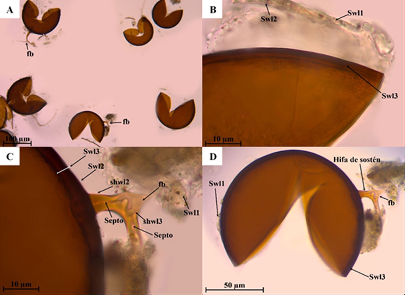
Figura 3. Estructura subcelular de Septoglomus furcatum A) Grupo de esporas, bifurcación de hifa (fb), característica de la especie en PVLG (10x); B) capas externas Swl1-3 en reactivo de Melzer (100x); C) capas externas Swl1-3 de la pared de la espora, capas Shwl1-2, septo y bifurcación de la hifa de sostén en reactivo de Melzer (100x); D) espora e hifa de sostén en PVLG (40x).
Esporas de color marrón rojizo a marrón oscuro; globosas de (106-) 138 (-167) µm de diámetro. La pared de la espora consta de 3 capas (Swl1-3). Capa Swl1, formando la superficie de la espora, semipermanente, hialina con restos de suelo de 1.6 µm de espesor y se desprende con la presión al oprimir el cubreobjetos. Swl2 semipermanente, hialina de 1.3 a 3.1 µm de espesor. Swl3 es laminada, lisa, marrón rojizo de 5.3 a 10.9 µm de espesor. Ninguna de las capas de la pared de la espora se tiñe con el reactivo de Melzer. La hifa de sostén es de color marrón parduzco; de forma recta de 10.5 a 30.3 µm, frecuentemente presenta una bifurcación (fb) a distancia de la pared de la espora. La pared de la hifa está compuesta de 3 capas (shwl1-3), las cuales son continuas a las paredes de la espora (Swl1-3). El poro de la espora está cerrado. El septo se encuentra en la base de la espora y pueden encontrarse numerosos septos a lo largo de la hifa.
Material examinado: México, Veracruz, Actopan, Plan de Higuera (19°26’17.0” N, 96°33’35.6” O, 140 m snm) en un suelo rizosférico de un bosque tropical caducifolio, H. Méndez-Cortés, 08-2020. México, San Luis Potosí, Matehuala (23°21’51.1” N, 100°35’01.7” O, 1,373 m snm) en un suelo rizosférico de matorral xerófilo, R. P. Hipólito-Piedras, 08-2021 (CH-SLPM-229).
Distribución y hábitat. Septoglomus furcatum, se registró por primera vez asociado a raíces de Cordia oncocalyx Allemann (Cordiaceae) en Brasil. Posteriormente se realizó un cultivo monoespecífico utilizando a Plantago lanceolata L. (Plantaginaceae) como planta huésped, en donde S. furcatum formó micorrizas con numerosos arbúsculos, vesículas e hifas poco frecuentes (Blaszkowski et al., 2013). El segundo reporte en Brasil, se evidenció a través de una investigación en torno a la retroalimentación de suelo-planta, donde la mencionan como una especie clave, propagada en Senna uniflora (Mill.) HSIrwin y Barneby (Caesalpiniaceae), con suelo de áreas degradadas que han sido restauradas en ese país (Medeiros et al., 2022). La presencia de S. furcatum en el continente asiático seregistró asociado a las raíces de Rosa acicularis Lindl. (Rosaceae) junto a una baja diversidad de 3 especies de HMA (Zu et al., 2019), mientras que Ming et al. (2023), la registraron en un bosque de Pinus damingshanensis W.C.Cheng y L.K.Fu (Pinaceae) , Cryptomeria japonica y en un bosque lanceolado de Cunninghamia R.Br. (Cupressaceae), junto con 27 especies más. En México, se aisló de suelo rizosférico de un bosque tropical caducifolio en Veracruz y matorral xerófilo en San Luis Potosí.
Septoglomus fuscum Błaszk., Chwat, Kovács y Ryszka, 2013.
Fig. 4a-d
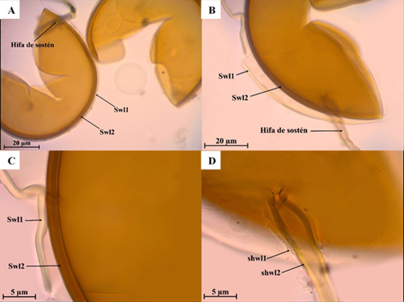
Las esporas se forman en el suelo en racimos sueltos. Grupos de 89-194 × 141-248 µm con 2 a 7 esporas. Esporas de color blanco amarillento en la juventud, anaranjado parduzco a marrón oscuro en la madurez; globosas a subglobosas; (32-) 51 (-102) µm de diámetro. La pared de la espora consta de 2 capas (Swl1-2). Swl1, es semipersistente, semiflexible, de color amarillo dorado, de 1.8 a 2.4 µm de grosor, al oprimir el cubreobjetos se separa de la capa Swl2. Swl2 es laminada, lisa, de amarillo a anaranjado parduzco de (1.8-) 3.5 (-6.7) µm de grosor. Ninguna de las capas de la pared de la espora se tiñe con el reactivo de Melzer. La hifa de sostén es de color anaranjado parduzco a marrón oscuro en esporas maduras; recta o recurvada, cilíndrica en forma de embudo, a veces ligeramente constreñida en la base de la espora; (5.8-) 7.4 (-12.3) µm de anchura en la base de la espora. Pared de la hifa de color amarillo a anaranjado parduzco de (0.8-) 2.7 (-5.8) µm de grosor. El poro es abierto de 1.5 a 2.7 µm de diámetro.
Material examinado: México, Veracruz, Actopan, Plan de Higuera (19°26’17.0” N, 96°33’35.6” O, 140 m snm) en un suelo rizosférico de un bosque tropical caducifolio, H. Méndez-Cortés, 08-2020. México, San Luis Potosí, Matehuala (23°21’51.1” N, 100°35’01.7” O, 1,373 m snm) en un suelo rizosférico de matorral xerófilo, R.P. Hipólito-Piedras, 08-2021 (CH-SLP-230).
Distribución y hábitat. Septoglomus fuscum se registró por primera vez asociado con raíces de Arctotheca populifolia (P.J.Bergius) Norl. (Asteraceae) en Sudáfrica. Posteriormente, se realizaron cultivos monoespecíficos con Plantago lanceolata como cultivo huésped, en donde se observaron estructuras como arbúsculos, hifas intra y extrarradicales (Blaszkowski et al., 2013). En México, se aisló de suelo rizosférico de bosque tropical caducifolio en Veracruz y un matorral xerófilo en San Luis Potosí.
Septoglomus turnauae Błaszk., Chwat, Ryszka y Orfanoudakis, 2014.
Fig. 5a-d
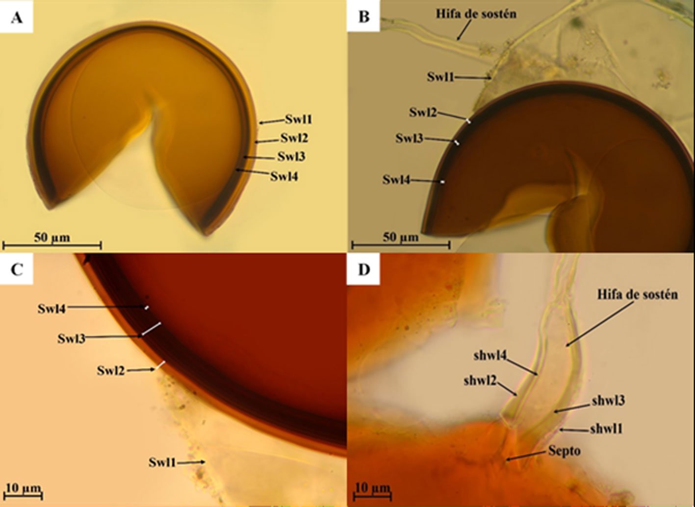
Las esporas se forman de manera solitaria en el suelo. Esporas de color anaranjado amarronado a marrón oscuro, globosas de (45) 64 (-102) µm de diámetro. La pared de la espora está compuesta de 4 capas (Swl1-4). Swl1, es evanescente, hialina, de 3.1 µm de diámetro. Swl2 es permanente, laminada, lisa, de anaranjado claro de 1.8 a 9.2 µm de espesor. Swl3 es laminada, lisa, de color anaranjado claro a anaranjado parduzco, de 3.5 a 9.3 µm de espesor. Swl4 semiflexible, lisa, de color anaranjado parduzco de 1.0 a 1.7 µm de espesor. Ninguna de las capas se tiñe con el reactivo de Melzer. La hifa es de color anaranjado parduzco de (4.5-) 8.2 (-10.7) µm de espesor en la base de la espora, la hifa es continua con las capas Swl1-3. El poro es de (1.3-) 2.7 (-3.2) µm de diámetro, estrechándose con la edad.
Material examinado: Coahuila, Sierra Hermosa (25°14’42” N, 100°51’18” O, 2,255 m snm) en suelo rizosférico de un bosque de pino, H. Méndez-Cortés, 08-2020. Guanajuato, San Felipe (21°41’56.4” N, 101°12’57.6” O, 2,445 m snm), en un suelo rizosférico de un bosque de encino, R.P. Hipólito-Piedras. San Luis Potosí, Xilitla (21°22’21.4” N, 99°00’39.0” O, 857 m snm) en un suelo rizosférico de un bosque mesófilo de montaña, R. P. Hipólito-Piedras, 08-2021. México, San Luis Potosí, Charcas (23°22’58.5” N, 101°20’18.5” O, 2,471 m snm) en un suelo rizosférico de un pastizal, R. P. Hipólito-Piedras, 08-2021. San Luis Potosí, Sierra de Álvarez (22°03’06.3” N, 100°34’50.8” O, 2,700 m snm) en un suelo rizosférico de un bosque de encino, R. P. Hipólito-Piedras, 08-2021. Tamaulipas, Jaumave (23°08’26.0” N, 99°17’48.4” O, 742 m snm) en un suelo rizosférico de un bosque de encino, R. P. Hipólito-piedras, 08-2021. (CH-SLPM-230).
Distribución y hábitat. S. turnuauae se registró en cultivos trampa inoculados con el suelo de la rizósfera y raíces de Cistus sp. L. (Cistaceae), en Italia. Posteriormente, se realizaron cultivos monoespecíficos con Plantago lanceolata, donde se observaron arbúsculos e hifas (Blaszkowski et al., 2014). En México, se aisló de suelo rizosférico de bosques de encino en Guanajuato y Tamaulipas, bosques de pino en Coahuila, bosque mesófilo de montaña y pastizal en San Luis Potosí.
Clave de las especies del género Septoglomus presentes en México
1. Esporas mayores a 200 micras 4
1. Esporas menores a 200 micras 2
2. Esporas con 2 capas en la pared de la espora 3
2. Esporas con 3 capas en la pared de la espora 5
2. Esporas con 4 capas en la pared de la espora 6
3 Esporas amarillas a marrones 7
3. Esporas rojas a negras 8
4. Esporas solitarias; de color anaranjado rojizo a marrón rojizo; globosa; (154.5-)202.8 (-228.9) µm de diámetro. La pared de la espora costa de 4 capas (Swl1-4). Capa Swl1 es evanescente hialina, lisa, con la edad se torna rugosa o se desprende. Swl2 permanente, laminada de color anaranjado, Swl3 es permanente, lisa y laminada de color anaranjado a marrón. Swl4 semiflexible, hialina, lisa, raramente se separa de swl3. Hifa de sostén amarilla a marrón, recurvada de 4 capas (shwl1-4), con poro cerrado por un septo situado en la base de la espora Septoglomus mexicanum
5. Esporas solitarias; de color marrón rojizo a marrón oscuro; globosas a subglobosas; (106-) 138 (-167) µm de diámetro. La pared de la espora consta de 3 capas (Swl1-3). Capa Swl1, semipermanente, hialina a anaranjado claro, lisa con gránulos de suelo. Swl2 semipermanente, hialina a amarillo dorado. Swl3 es laminada, lisa, marrón rojizo a marrón oscuro. La hifa de sostén es de color marrón parduzco a marrón oscuro; rectas o curvadas, cilíndricas, bifurcada, compuestas por 3 capas (shwl1-3), poro cerrado por un septo en la base de la espora, además, a lo largo de la hifa se encontrarán septos transversales Septoglomus furcatum
6. Esporas solitarias; de color anaranjado parduzco a marrón oscuro; globosas a subglobosas; (110-) 133(-165) μm de diámetro. La pared de la espora consta de 4 capas (Swl1-4). Swl1, es evanescente, hialina y lisa. Swl2 permanente, laminada, lisa, de color anaranjado claro a anaranjado parduzco. Swl3 es laminada, lisa, de color anaranjado claro a anaranjado parduzco. Swl4 semiflexible, lisa, de color anaranjado claro a anaranjado parduzco. La hifa de sostén es de color anaranjado parduzco a marrón oscuro, constituida de 3 capas (shwl1-3) con un septo en la base de la espora que no invade el lumen de la hifa de sostén Septoglomus turnauae
7. Esporas en racimos o solitarias, de color amarillento en la juventud, anaranjado parduzco a marrón oscuro en la madurez; globosas a subglobosas; (20- ) 47 (-90) µm de diámetro. La pared de la espora consta de 2 capas (Swl1-2). Swl1, semi persistente, semiflexible, de color blanco anaranjado a amarillo dorado. Swl2 laminada, lisa, blanco amarillento en esporas juveniles, anaranjado parduzco a marrón oscuro en esporas maduras. La hifa de sostén de color anaranjado parduzco a marrón oscuro; recta o recurvada, cilíndrica a forma de embudo, con poro abierto, sin septo, estrechamiento gradual hasta llegar al centro del lumen de la hifa Septoglomus fuscum
8. Esporas solitarias; de color marrón rojizo oscuro a negro rojizo; ovoides, elípticas y globosas, de 137-175 (-208) × 125-170 (-204) µm de diámetro. La pared de la espora está compuesta por 2 capas (Swl1-2). Swl1 es subhialina, lisa, de color amarillo oscuro. Swl2 es de marrón rojizo oscuro a negro rojizo, lisa, laminada. La hifa de sostén de color amarillo oscuro a un marrón rojizo, cilíndrica, curveada, ancha en la base de la espora estrechándose debajo de esta, poro cerrado, septo concoloro a la base de la espora y tonalidad clara cuando se encuentra debajo de la pared de la espora Septoglomus altomontanum
Discusión
En México, el género Septoglomus está representado por 33% de las especies descritas en el mundo, lo que equivale a 5 de las 13 especies conocidas. Entre éstas, destaca S. constrictum debido a su amplia distribución y frecuentes registros en diversas comunidades vegetales. Por otro lado, S. xanthium ha sido principalmente registrada en agroecosistemas (Polo-Marcial et al., 2021). Septoglomus mexicanum se ha registrado en asociación con Prosopis laevigata (Humb. y Bonpl. ex Willd.) M.C.Johnst. (Mimosaceae) (Chimal-Sánchez et al., 2020), similar a S. titan BT Goto y GA Silva (Glomeraceae) que se ha registrado en zonas áridas del país (Guardiola-Márquez et al., 2022).
De acuerdo con los registros de las especies de HMA descritas en esta investigación, Septoglomus altomontanum fue la única especie cuya distribución coincidió con la descripción original al ser aislada en sitios con vegetación de coníferas y encinos, a altitudes superiores a 2,000 m, lo cual es similar a lo reportado por Palenzuela et al. (2013), quienes documentaron su presencia en zonas con vegetación similar, localizadas entre 1,800 y 3,100 m de altitud.
Septoglomus altomontanum se diferencia de las especies de HMA descritas hasta la fecha, incluso de las del mismo género, en términos de tamaño, color, estructura, forma e hifas de las esporas. La especie que podría generar algún debate conforme a su morfología es S. furcatum; no obstante, ésta presenta la particularidad de tener una hifa que se adelgaza a medida que se aleja de la base de la espora (Blaszkowski et al., 2013), mientras que S. altomontanum mantiene un grosor uniforme a lo largo de la pared de la espora y la hifa (Palenzuela et al., 2013).
Septoglomus furcatum se destaca por sus esporas grandes de tonalidad oscura que presentan una pared de 3 capas y, con frecuencia, hifas ramificadas, incluso llegando a tener 2 hifas cercanas entre sí, característica que no se encuentra en otras especies del género Septoglomus (Blaszkowski et al., 2013).A primera vista, las esporas de S. furcatum pueden parecer similares a las de S. constrictum (Trappe) Sieverd., GA Silva et Oehl; sin embargo, se diferencian por la estructura de la pared de la espora, ya que S. furcatum tiene 3 capas, mientras que S. constrictum tiene solo 2. Además, la espora de S. constrictum tiende a ser de un tono anaranjado parduzco, mientras que la de S. furcatum es de color marrón oscuro. La característica de S. furcatum de poseer una hifa ramificada, es similar a la de las esporas de G. brohultii Sieverd. y R.A. Herrera (Glomeraceae). Sin embargo, G. brohultii tiene una tonalidad más clara tanto en la pared de la espora como en la hifa, a diferencia de S. furcatum, que presenta una tonalidad oscura uniforme tanto en la pared como en la hifa (Blaszkowski et al., 2013; Oehl et al., 2011).
Septoglomus fuscum es similar a S. xanthium, tanto en características moleculares como en características morfológicas. No obstante, se ha observado que S. fuscum forma racimos sueltos de esporas, mientras que S. xanthium se compone de esporas solitarias que se adhieren y se desarrollan dentro de las raíces (Blaszkowski et al., 2004). Al analizar las capas, se nota que S. xanthium posee una capa adicional permanente que S. fuscum no presenta; sin embargo, S. fuscum tiene un grosor de capa laminada de 2 a 3 veces mayor que el de S. xanthium (Blaszkowski et al., 2013).
Desde una perspectiva filogenética, S. turnauae presenta una estrecha relación con S. fuscum, lo que sugiere un origen común entre ambas especies, a través de análisis ribosomales que las agrupan en un mismo clado. Sin embargo, se destaca que la mayoría de las esporas de S. fuscum se agrupan en racimos sueltos (Blaszkowski et al., 2013), en contraste con las esporas individuales de S. turnauae. Al comparar el número de capas, S. turnauae muestra similitudes con S. mexicanum, ambas compuestas por 4 capas en su estructura, aunque, difieren en el color de las esporas. Mientras que S. mexicanum presenta tonalidades que van desde el rojizo hasta el marrón (Chimal-Sánchez et al., 2020), las esporas de S. turnauae tienen un tono anaranjado parduzco y tonalidades diferentes, conforme empieza otra capa (Blaszkowski et al., 2014).
Previo a esta investigación, se consideraba que la distribución del género Septoglomus era limitada, sin embargo, donde se localiza expresa un comportamiento dominante respecto a los demás géneros de HMA (Guardiola-Márquez et al., 2022). No obstante, la presente investigación, que ha registrado 4 especies pertenecientes a este género, revela una riqueza de HMA previamente desconocida en las comunidades vegetales de México. Además, sugiere que este género no se encuentra restringido a una distribución específica, ya que se ha documentado en 5 comunidades vegetales distintas en el país. El reciente hallazgo de S. altomontanum, S. fuscum, S. furcatum y S. turnauae eleva el número de especies registradas en México a 171, ésto constituye aproximadamente 48% de la riqueza global de HMA y 62% de las especies se han reportado del género Septoglomus en el país.
Agradecimientos
A la Secretaría de Ciencia, Humanidades, Tecnología e Innovación (Secihti) por la beca otorgada (775694) a la primera autora para sus estudios de posgrado.
Referencias
Błaszkowski, J., Blanke, V., Renker, C., y Buscot, F. (2004). Glomus aurantium and G. anthium, new species in Glomeromycota. Mycotaxon, 90, 447–467. https://doi.org/10.5962/p.431247
Błaszkowski, J., Chwat, G., Góralska, A., Ryszka, P. y Orfanoudakis, M. (2014). Septoglomus jasnowskae and Septoglomus turnauae, two new species of arbuscular mycorrhizal fungi (Glomeromycota). Mycology Progress, 13, 985. https://doi.org/10.1007/s11557-014-0985-z
Blaszkowski, J., Chwat, G., Kovacs, G. M., Gaspar, B. K., Ryszka, P., Orowska, E. et al. (2013). Septoglomus fuscum and S. furcatum, two new species of arbuscular mycorrhizal fungi (Glomeromycota). Mycologia, 105, 670–680. https://doi.org/10.3852/12-127
Błaszkowski, J., Kovács, G. M., Balazs, T. K., Orlowska, E., Sadravi, M., Wubet, T. et al. (2010). Glomus africanum and G. iranicum, two new species of arbuscular mycorrhizal fungi (Glomeromycota). Mycologia, 102, 1450–1462. https://doi.org/10.3852/09-302
Błaszkowski, J., Yamato, M., Niezgoda, P., Zubek, S., Milczarski, P., Malinowski, R. et al. (2023). A new genus, Complexispora, with two new species, C. multistratosa and C. mediterranea, and Epigeocarpum japonicum sp. nov. Mycological Progress, 22, 1–15. https://doi.org/10.1007/s11557-023-01882-9
Chimal-Sánchez, E., Senés-Guerrero, C., Varela, L., Montaño, N. M., García-Sánchez, R., Pacheco, A. et al. L. (2020). Septoglomus mexicanum, a new species of arbuscular mycorrhizal fungi from semiarid regions in Mexico. Mycologia, 112, 121–132. https://doi.org/10.1080/00275514.2019.1671147
Conabio (Comisión Nacional para el Conocimiento y Uso de la Biodiversidad). (2018). Sistema Nacional de Información sobre Biodiversidad (SNIB). Registros de ejemplares, versión 2017-12. Geoportal y Enciclovida, México. Recuperado el 28 julio, 2023 de: http://www.conabio.gob.mx/informacion/gis/
da Silva, G. A., Corazon-Guivin, M. A., de Assis, D. M. A. y Oehl, F. (2023). Blaszkowskia, a new genus in Glomeraceae. Mycological Progress, 22, 1–14. http://dx.doi.org/10.1007/s11557-023-01919-z
Daniels, H. B. A. y Skipper, H. D. (1982). Methods for the recovery and quantitative estimation of propagules from soil. En N. C. Schenck (Ed.), Methods and principles of mycorrhizal research (pp. 29–37). St. Paul, Minn.: American Society for Phytopathology,
Gerdemann, J. W. y Nicolson, T. J. (1963). Spores of mycorrhizal Endogonespecies extracted from soil by wet sieving and decanting. Transactions of the British Mycological Society, 46, 235–244. http://dx.doi.org/10.1016/S0007-1536(63)80079-0
Goto, B. T., Araújo, A. F., Soares, A. C. F., de Almeida-Ferreira, A. C., Maia, L. C., da Silva-Sousa, C. et al. (2013). Septoglomus titan, a new fungus in the Glomeraceae (Glomeromycetes) from Bahia, Brazil. Mycotaxon, 124, 101–109. http://dx.doi.org/10.5248/124.101
Guardiola-Márquez, C. E., Pacheco, A., Mora-Godinez, S., Schüßler, A., Gradilla-Hernández, M. S. y Senés-Guerrero, C. (2022). Septoglomus species dominate the arbuscular mycorrhiza of five crop plants in an arid region of northern Mexico. Symbiosis, 87, 93–106. http://dx.doi.org/10.1007/s13199-022-00851-2
Guillén, A., Serrano-Tamay, F. J., Peris, J. B. y Arrillaga, I. (2020). Glomus ibericum, Septoglomus mediterraneum, and Funneliformis pilosus, three new species of arbuscular mycorrhizal fungi. Mycologia, 112, 819–828. https://doi.org/10.1080/00275514.2020.1771992
He, R. J., Ming, Y., Yao, L. M., Zhu, Q. Q. y Jiang, L. (2021). Diversity of arbuscular mycorrhizal fungi in mossy dwarf forest of Fanjing Mountain, Guizhou Province, Southwest China. Mycosystema, 40, 2843–2853. https://doi.org/10.13346/j.mycosystema.210188
INVAM (International Culture Collection of Vesicular Arbuscular Mycorrhizal Fungi). (2023). Recuperado el 28 agosto, 2023 de: http://invam.caf.wvu.edu/
Khaekhum, S., Lumyong, S., Kuyper, T. W. y Boonlue, S. (2017). Species richness and composition of arbuscular mycorrhizal fungi occurring on eucalypt trees (Eucalyptus camaldulensis Dehnh.) in rainy and dry season. Current Research in Environmental and Applied Mycology, 7, 282–292. http://dx.doi.org/10.5943/cream/7/4/5
Medeiros, A. S., Scaloppi, J. C., Damasceno, E. S., Goto, B. T., Vieira, D. C. M., Socolowski, F. et al. (2022). Arbuscular mycorrhizal fungi communities shaped by host-plant affect the outcome of plant-soil feedback in dryland restoration. Journal of Applied Ecology, 60, 507–518. https://doi.org/10.1111/1365-2664.14330
Ming, Y., He, R., Yao, L., Zhu, Q., Long, C. y Jiang, L. (2023). Diversity of soil arbuscular mycorrhizal fungi in different coniferous forests in Fanjing Mountain. Journal of Yunnan Agricultural University (Natural Science), 38, 149–157. https://doi.org.10.12101/j.issn.1004-390X(n).202108033
Niezgoda, P., Błaszkowski, J., Błaszkowski, T., Stanisławczyk, A., Zubek, S., Milczarski, P. et al. (2024). Three new species of arbuscular mycorrhizal fungi (Glomeromycota) and Acaulospora gedanensis revised. Frontiers in Microbiology, 15, 1320014. https://doi.org/10.3389/fmicb.2024.1320014
Oehl, F., Sánchez-Castro, I., da Silva, D. K. A., Santos, V. M., Palenzuela Jiménez, E. J. y da Silva, G. A. (2019). Septoglomus nigrum, a new arbuscular mycorrhizal fungus from France, Germany and Switzerland. Nova Hedwigia, 109, 121–134. http://dx.doi.org/10.1127/nova_hedwigia/2019/0523
Oehl, F., Silva, G. A. D., Goto, B. T. y Sieverding, E. (2011). Glomeromycota: three new genera and glomoid species reorganized. Mycotaxon, 116, 75–120. http://dx.doi.org/10.5248/116.75
Palenzuela, J., Azcón-Aguilar, C., Barea, J. M., da Silva, G. A. y Oehl, F. (2013). Septoglomus altomontanum, a new arbuscular mycorrhizal fungus from mountainous and alpine areas in Andalucía (southern Spain). IMA Fungus, 4, 243–249. https://doi.org/10.5598/imafungus.2013.04.02.09
Polo-Marcial, M. H., Lara-Pérez, L. A., Goto, B. T., Margarito-Vista, X. y Andrade-Torres A. (2021). Glomeromycota in Mexico, a country with very high richness. Sydowia, 74, 33–63. http://dx.doi.org/10.12905/0380.sydowia74-2021-0033
Redecker, D., Schüßler, A., Stockinger, H., Stürmer, S. L., Morton, J. B. y Walker, C. (2013). An evidence-based consensus for the classification of arbuscular mycorrhizal fungi (Glomeromycota). Mycorrhiza, 23, 515–531. https://doi.org/10.1007/s00572-013-0486-y
Schüßler, A., Schwarzott, D. y Walker, C. (2001). A new fungal phylum, the Glomeromycota: phylogeny and evolution. Mycological Research, 105, 1413–1421. https://doi.org/10.1017/S0953756201005196
Schüßler, A. y Walker, C. (2010). The Glomeromycota. A species list with new families and new genera. Recuperado el 28 agosto, 2023 de: http://schuessler.userweb.mwn.de/amphylo/
Symanczik, S., Błaszkowski, J., Chwat, G., Boller, T., Wiemken, A. y Al-Yahya’ei, M. N. (2014). Three new species of arbuscular mycorrhizal fungi discovered at one location in a desert of Oman: Diversispora omaniana, Septoglomus nakheelum and Rhizophagus arabicus. Mycologia, 106, 243–259. https://doi.org/10.3852/106.2.243
Zu, Y., Ping, Y., Mu, L. y Yang, T. (2019). The diversity of arbuscular mycorrhizal fungi of Rosa acicularis ‘Luhe’in saline areas. Journal of Forestry Research, 30, 1507–1512. https://doi.org/10.1007/s11676-018-0748-9
Wijayawardene, N. N., Hyde, K. D., Al-Ani, L. K. T., Tedersoo, L., Haelewaters, D., Rajeshkumar, K. C. et al. (2020). Outline of fungi and fungus-like taxa. Mycosphere Online. Journal of Fungal Biology, 11, 1060–1456. https://doi.org/10.5943/mycosphere/13/1/2
Schüβler, A. 2025. Glomeromycota: species list. Recuperado en marzo, 2025 de: http://www.amf-phylogeny.com/

Morfología del huevo y comportamientos de oviposición en Pseudosermyle (Phasmatodea: Diapheromeridae)
Egg morphology and oviposition techniques in Pseudosermyle (Phasmatodea: Diapheromeridae)
Ulises López-Mora a, b, *, Enrique González-Soriano a, A. Celeste Martínez-Cervantes a, b, Jorge Llorente-Bousquets c
a Universidad Nacional Autónoma de México, Instituto de Biología, Departamento de Zoología, Tercer Circuito Universitario s/n, Ciudad Universitaria, Coyoacán, 04510 Ciudad de México, México
b Universidad Nacional Autónoma de México, Posgrado en Ciencias Biológicas, Instituto de Biología, Departamento de Zoología, Tercer Circuito Universitario s/n, Ciudad Universitaria, Coyoacán, 04510 Ciudad de México, México
c Universidad Nacional Autónoma de México, Facultad de Ciencias, Departamento de Biología Evolutiva, Museo de Zoología Alfonso L. Herrera, Circuito Exterior s/n, Ciudad Universitaria, Coyoacán, 04510 Ciudad de México, México
* Autor para correspondencia: nxitl00@gmail.com (U. López-Mora)
Recibido: 30 julio 2025; aceptado: 04 octubre 2025
Resumen
Pseudosermyle es el género de insectos palo con mayor riqueza en América del Norte; muestra una distribución desde el sur de los EUA hasta América Central, desafortunadamente ha sido poco estudiado. En el presente trabajo se realiza la primera aproximación en extenso a la morfología del huevo en Pseudosermyle respecto a su microestructura, con el empleo de microscopía electrónica de barrido (MEB), así como el análisis de componentes principales para determinar la utilidad de las medidas estandarizadas que se utilizan en la descripción de huevos, además de su ornamentación. Se encontraron 4 patrones en el huevo de Pseudosermyle, entre los que se incluyen 3 tipos de oviposición: liberación, adheridos al sustrato y formación de ooteca. Esto sugiere que podría tratarse de géneros distintos bajo una posible subtribu. Además, la ornamentación del huevo es lo suficientemente distinta para reconocer diferentes especies. Por lo tanto, se debe analizar la importancia de estos caracteres en la descripción de especies de Pseudosermyle.
Palabras clave: Diapheromerinae; Diapheromerini; Phasmida; MEB; Insectos palo
Abstract
Pseudosermyle is the genus of stick insects with the greatest diversity in North America, with a range extending from the southern USA to Central America; unfortunately, it has been poorly studied. In this work, we present the first comprehensive analysis of the egg morphology in Pseudosermyle in relation to ultrastructure, using scanning electron microscopy, along with principal component analysis to evaluate the effectiveness of the standardized measurements used in the egg descriptions, as well as the ornamentation. We identified 4 general patterns in Pseudosermyle eggs corresponding to 3 different oviposition techniques: dropping, attaching to substrate and forming oothecae. These patterns suggest the possibility of recognizing different genera within a putative subtribe. Additionally, the ornamentation is sufficiently distinct to differentiate among species. Thus, we emphasize the importance of these characters in the description of species of Pseudosermyle.
Keywords: Diapheromerinae; Diapheromerini; Phasmida; SEM; Stick insects
Introducción
El orden Phasmatodea comprende organismos denominados insectos palo, hoja o corteza. Por lo general se reconocen por su cuerpo alargado y cilíndrico o deprimido; es menos frecuente encontrar formas más robustas (Bradler y Buckley, 2018). Su coloración varía en distintos matices del castaño al verde, aunque existen algunos con coloraciones aposemáticas (rojo, amarillo o azul). En la etapa adulta ninguno de estos insectos mide menos de 2 cm de longitud (Seiler et al., 2006). Una característica notoria es su cripsis con la vegetación, que en conjunto con comportamientos especializados, como la catalepsia e imitación del balanceo de las hojas y el follaje durante el día (Bradler y Buckley, 2018), les permiten pasar inadvertidos frente a sus depredadores. Sus huevos se asemejan a semillas de las plantas donde habitan (Severin, 1910).
La ootaxonomía de Phasmatodea se estandarizó con los trabajos de Clark (1976a, b, 1979) y Sellick (1994, 1997a, b, 1998). A partir de entonces, el huevo se ha incluido en las descripciones de sus especies (Allred et al., 1986; Conle et al., 2007; López-Mora y Llorente-Bousquets, 2023) y también se han efectuado trabajos utilizando el microscopio electrónico de barrido (MEB) para el análisis de las microestructuras y la textura de la cápsula en especies pertenecientes a los géneros Agathemera Stål, 1875, Anisomorpha Gray, 1835, Bacillus Berthold, 1827, Burria Brunner von Wattenwyl, 1900, Carausius Stål, 1875, Clonopsis Pantel, 1915, Heteronemia Gray, 1835, Lonchodes Gray, 1835, Megaphasma Caudell, 1903, Orxines Stål, 1875, Paraprisopus Redtenbacher, 1906, Ramulus Saussure, 1862, Sipyloidea Brunner von Wattenwyl, 1893, Timema Scudder, 1895 y Xeropsis Redtenbacher, 1906 (Allred et al., 1986; Camousseight y Bustamante, 1991; Jintsuet al., 2010; Mazzini y Scali, 1977, 1980, 1983; Mazzini et al., 1982, 1984, 1992; Scali y Mazzini, 1977, 1981, 1982, 1983; Stark y Lentz, 1986). En particular, la textura de la cápsula y la ornamentación del opérculo han resultado ser muy útiles en la diferenciación de especies cercanamente relacionadas (Mazzini et al., 1982, 1992; Scali y Mazzini, 1981), incluso para diferenciar híbridos (Mazzini et al., 1984). En suma, los trabajos previos han concluido en la importancia de los estudios con MEB y microscopia óptica para la diferenciación entre especies cercanamente relacionadas en Phasmatodea y posibles híbridos.
Pseudosermyle Caudell, 1903 es el género más diverso en México y América del Norte, con 26 especies en total (de Luna, 2022; López-Mora y Llorente-Bousquets, 2018). Sin embargo, solo se conocen 4 ilustraciones, que no son de microestructura del huevo, para 3 especies: Pseudosermyle tridens (Burmeister, 1838), ilustrada por Kaup (1871) y Zompro (2001); P. truncata Caudell, 1903, por Caudell (1914) y P. phalangiphora Conle, Hennemann et Fontana, 2007, por ellos mismos. Al observar las imágenes de estas 3 especies se advierten diferencias significativas en las formas de la cápsula y la lámina micropilar, que no han sido evaluadas en su microestructura y son relevantes para distinguir especies.
Nuestro objetivo fue realizar una exploración más extensa sobre la morfología coriónica a nivel de microestructura utilizando MEB, incorporando 11 especies más de Pseudosermyle, así como analizar su empleo a nivel genérico y específico al reconocer jerarquías entre los caracteres que se utilizan para describir a las especies.
Materiales y métodos
Los acrónimos y abreviaturas de las colecciones son: CNIN = Colección Nacional de Insectos, Instituto de Biología, UNAM; MZFC = Museo de Zoología Alfonso L. Herrera, Facultad de Ciencias, UNAM. Estructuras coriónicas: H = altitud de la cápsula; L = longitud de la cápsula; mpi = lámina micropilar interna; mpl = longitud de la lámina micropilar; mpw = amplitud de la lámina micropilar, NM = lámina micropilar interna abierta con línea media; oph = altura del opérculo, opw = amplitud del opérculo; PO = lámina micropilar interna paralela sin línea media; W = amplitud de cápsula; %h/l = índice de elongación, %w/h = índice de compresión.
Se recolectaron 44 machos y 61 hembras en distintas localidades (fig. 1, tabla 1) y se depositaron en la CNIN y MZFC (tabla 2), Nooxapty isabelae se revisó de los ejemplares tipos depositados en las colecciones por López-Mora y Llorente-Bousquets (2023) (tabla 2). Los ejemplares que se obtuvieron de crianza aún no se depositan en colección alguna, pues se están utilizando para otro tipo de estudios. Los puntos de recolecta se muestran en un mapa (fig. 1) obtenido con QGIS 3.8.1-Zanzibar (QGIS, 2019). Para obtener los huevos, se seleccionaron 22 hembras de distintas especies (tabla 3), el número de hembra varió entre las especies pues algunas no sobrevivieron al traslado, se mantuvieron en cautiverio y aisladas entre sí (dentro de diferentes contenedores) con las siguientes condiciones: temperatura de 20-22 °C, humedad relativa 60-80%, alimentación con base en Galinsoga sp. (Asteraceae) que se colocó en frascos con agua. Estuvieron bajo ciclos de luz y oscuridad correspondientes a los presentados en la CDMX durante el lapso que estuvieron cautivas; se intentaron replicar las condiciones de temperatura y humedad tomadas en campo con un termohigrómetro digital PEAKMETER PM6508. Los organismos se identificaron comparando la morfología de adultos (machos y hembras) y el tipo de oviposición, en particular con las fotografías e ilustraciones de Brock et al. (2019), estos datos fueron cualitativos y no se incluyeron en el análisis de componentes principales (PCA). Para Nooxapty isabelae López-Mora et Llorente-Bousquets, 2023 se examinaron los huevos de la serie tipo y se usó como grupo externo. Se observaron y midieron en total 255 huevos de 22 hembras de 12 especies (tabla 3) bajo un microscopio Olympus SZX12, con ocular de reglilla micrométrica y un objetivo Olympus DF PL 1.5 X-4. Se efectuaron las mediciones de los huevos acorde con Sellick (1997b); los datos se presentan en las tablas 4-9 y en las diagnosis se expresan las cifras bajo los siguientes parámetros estadísticos: n = tamaño de la muestra, promedio ± desviación estándar (valor mínimo-valor máximo) en las descripciones.
Tabla 1
Localidades de recolecta de las distintas especies de insectos palo, el orden es alfabético por estado.
| Localidad | Longitud | Latitud | Especies |
| REPSA, Coyoacán, Ciudad de México, México | 19.317634 | -99.184854 | Pseudosermyle sp. 2 |
| Arriba cueva, Valle de Bravo, Estado de México | 19.09248 | -100.07218 | Pseudosermyle sp. 1 |
| Bajo mesa, Valle de Bravo, Estado de México, México | 19.0861 | -100.07665 | Pseudosermyle carinulata |
| Villa Esmeralda, Silao, Guanajuato, México | 20.95367 | -101.43361 | Pseudosermyle sp. 4 |
| EBCH, La Huerta, Jalisco, México | 19.49931 | -105.04484 | Pseudosermyle sp. 3 |
| Cruz Verde, Ayala, Morelos, México | 18.760174 | -98.976098 | Pseudosermyle tridens |
| Curva Choápam-Latani, Santiago Choápam, Oaxaca, México | 17.377754 | -95.916254 | Pseudosermyle sp. 6 |
| Curva 1 Amatepec-Chinantequilla, Totontepec Villa de Morelos, Oaxaca, México | 17.28485 | -95.988362 | Nooxapty isabelae |
| Camino a Tzinacapan, Cuetzalan, Puebla, México | 20.016558 | -97.53983 | Pseudosermyle striatus Psudosermyle sp. 5 |
| EBTLT, San Andrés Tuxtla, Veracruz, México | 18.5860833 | -95.0755 | Pseudosermyle phalangiphora Pseudosermyle procera |
Tabla 2
Organismos revisados y depositados en las colecciones por especie, sexo y huevos indicando el voucher. Para Nooxapty isabelae se indican los ejemplares revisados. En Núm. de especímenes se separan los ejemplares depositados y revisados (primera cifra) de los revisados (segunda cifra) por un símbolo de más “+”.
| Especie | CNIN | MZFC | ||||
| Machos | Hembras | Huevos | Machos | Hembras | Huevos | |
| Pseudosermyle sp. 1 | PHMX351-354, 356-358 | PHMX26 | PHMX125 | PHMX349-350, 355, 426 | ||
| Tabla 2. Continúa | ||||||
| Especie | CNIN | MZFC | ||||
| Machos | Hembras | Huevos | Machos | Hembras | Huevos | |
| Pseudosermyle sp. 2 | PHMX307-308, 311, 314-322 | PHMX72-75, 78-79 | PHMX76-77, 80 | PHMX304-306, 309-310, 312-313 | ||
| Pseudosermyle sp. 3 | PHMX467-468 | PHMX469-471 | PHMX324, 327-328 | PHMX323, 325-326 | ||
| P. tridens | PHMX678 | PHMX679-680 | PHMX332-337, 341, 343-348, 616-618 | PHMX329-331, 338-340, 342 | ||
| Pseudosermyle sp. 4 | PHMX91, 93 | PHMX94-100 | PHMX362-365, 367-373, 423-425 | PHMX54-56, 90, 92 | PHMX57-62 | PHMX359-361, 366 |
| P. carinulata | PHMX160-163 | PHMX164-165, 168, 653 | PHMX420-421 | PHMX416-419, 422 | ||
| P. striata | PHMX81-85 | PHMX86-89 | PHMX262-270, 272-273, 277-288, 292-300, 302-303 | PHMX463 | PHMX462, PHMX464-465 | PHMX259-261, 271, 274-276, 289-291, 301 |
| Pseudosermyle sp. 5 | PHMX27 | PHMX378-388 | PHMX1-2, 11-12 | PHMX4-6, 13 | PHMX374-377 | |
| P. phalangiphora | PHMX101-102, 135, 148, 155 | PHMX103-107, 146-147, 149 | PHMX172-183, 188-198, 203-213 | PHMX169-171, 184-187, 199-202 | ||
| P. procera | PHMX108-110, 136-137, 151, 156-157 | PHMX111-114, 150, 152-154, | PHMX217-228, 232-243, 248-258 | PHMX214-216, 229-231, 244-247 | ||
| Pseudosermyle sp. 6 | PHMX681 | PHMX405-415 | PHMX401-404 | |||
| Nooxapty isabelae | PHMX117, 119 | PHMX115 | PHMX389-393, 399-400 | PHMX118 | PHMX116 | PHMX394-398 |
| Núm. especímenes | 27+2 | 38+1 | 179+7 | 17+1 | 23+1 | 70+5 |
Tabla 3
Especies de Phasmatodea revisadas, número de hembras por especie tentativamente bajo el género Pseudosermyle y número de huevos por hembra revisados.
| Especies de Phasmatodea revisadas | Clave | Huevos por hembra | ||
| Nombre | Clave de ♀ | Núm. de ♀ | ||
| Pseudosermyle sp. 1 | PtgVB | U | 1 | 11 |
| Pseudosermyle sp. 2 | PtgDF | G1 G2 | 1 2 | 5 14 |
| Pseudosermyle sp. 3 | Pch | F1 F2 | 1 2 | 3 3 |
| P. tridens | PtrMor | T1 T2 | 1 2 | 10 10 |
| Tabla 3. Continúa | ||||
| Especies de Phasmatodea revisadas | Clave | Huevos por hembra | ||
| Nombre | Clave de ♀ | Núm. de ♀ | ||
| Pseudosermyle sp. 4 | PtrGto | U | 1 | 15 |
| P. carinulata | Pca | C1 C2 | 1 2 | 5 2 |
| P. striata | Pst | S1 S2 S3 | 1 2 3 | 15 15 15 |
| Pseudosermyle sp. 5 | PspF | U | 1 | 15 |
| P. phalangiphora | Pph | H1 H2 H3 | 1 2 3 | 15 15 15 |
| P. procera | Ppr | P1 P2 P3 | 1 2 3 | 15 15 15 |
| Pseudosermyle sp. 6 | Poax | U | 1 | 15 |
| N. isabelae | Nisa | U | 1 | 12 |
| Total: 12 spp. | — | — | 22 | 255 |
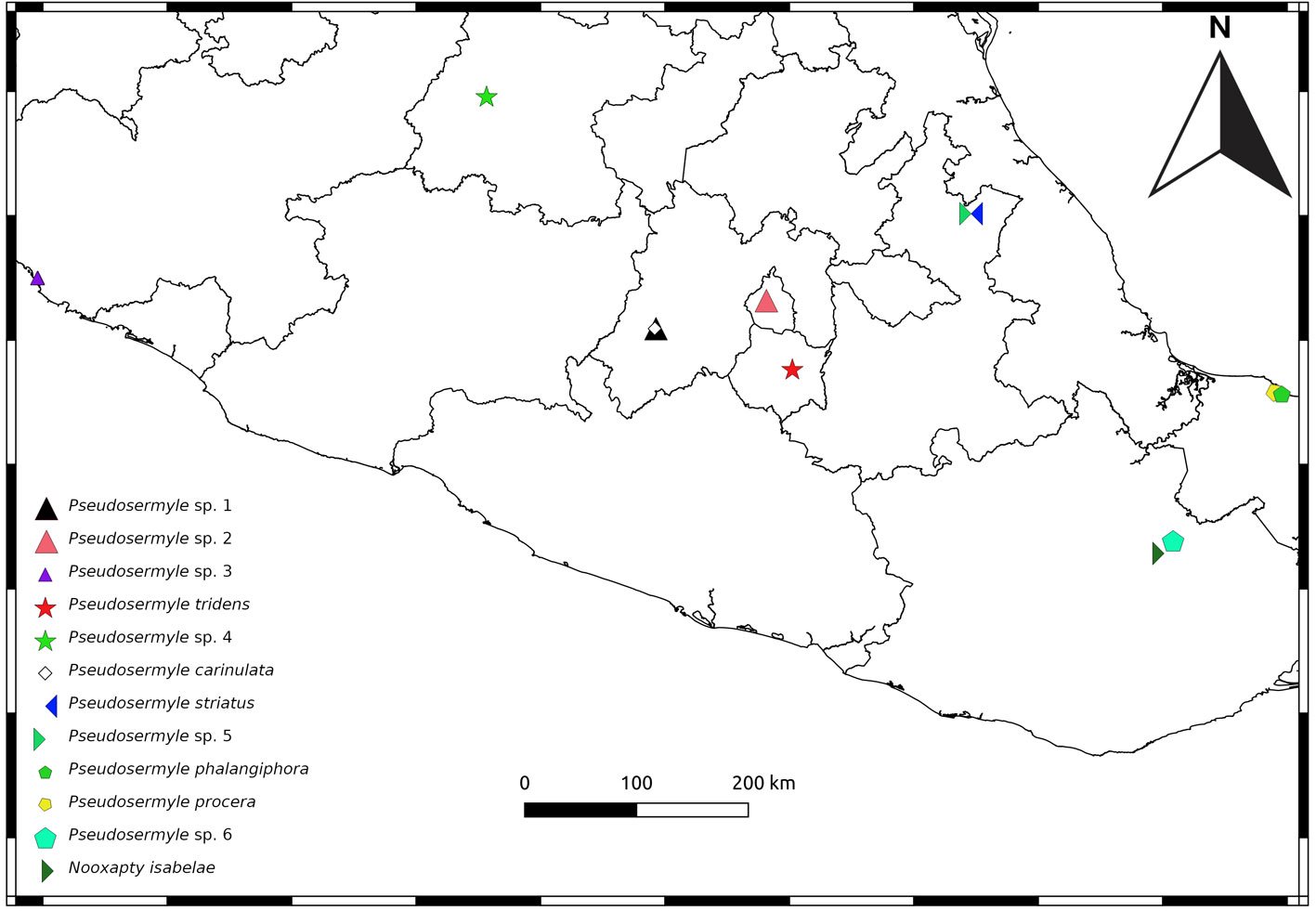
Para asociar machos con hembras que no se encontraban en cópula en el campo, se realizaron los siguientes pasos: a) se observaron los machos con los cuales copulaban las hembras en cautiverio; b) se separaron los huevos por morfología y hembra; c) éstos se incubaron por separado; d) cuando eclosionaron, las ninfas se mantuvieron en terrarios separados; e) se obtuvieron adultos y se comparó la morfología con la presentada por los parentales; f) cuando se obtienen machos y hembras de la misma hembra se corrobora si la morfología que presentan es similar a la de los parentales y se deduce qué machos parentales coinciden; g) se observa que los machos copulen con las hembras correspondientes con la morfología materna; y h) se compara la morfología coriónica de los huevos de las hembras hijas con las parentales para corroborar la correspondencia. Estos pasos permiten discernir cuando hay especies del mismo género que se encuentran en el mismo sitio, o cuando desconocemos la correspondencia entre sexos en los insectos palo de una localidad.
Se tomaron micrografías con una cámara de 8MP LEICA DFC490 adaptada a un microscopio LEICA Z16 AP0A y obtenidas con Leica Application Suite. Éstas se procesaron con GIMP 2.8.22 (GNU). Se llevaron a cabo observaciones bajo el MEB, los huevos se procesaron modificando el método de Nieves-Uribe et al. (2021) de la siguiente manera: serie descendente de etanol, 10 min en cada uno (96% → 70% → 50% → 30% → 10%) → H2O destilada (10 min) → jabón biológico (agitación manual constante) → Sonicar por 10 seg en 2 lapsos de 5 seg (con un sonicador modelo: Bronson 200) → enjuagar en agua destilada → agua destilada (10 min) → serie ascendente de etanol, 10 min en cada uno (10% → 30% → 50% → 70% → 96%) → dejar evaporar el alcohol (30 min. aprox.) → montar la muestra → dejar secar por 2 días en un recipiente hermético con una bolsita de silica gel (2 días). Las muestras se cubrieron en la ionizadora 19Quorum 150R ES en 2 ciclos de 20 min cada uno y se observaron bajo un microscopio Hitachi SU3500. Las abreviaturas en las medidas del huevo siguen la nomenclatura de Sellick (1997b, c, 1998). Las estructuras descritas y propuestas para el huevo se ilustran en la figura 2. Se siguió la nomenclatura de texturas de Harris (1979) para las descripciones de microestructura, en este caso solo se midieron las estructuras de 1 huevo por especie por el costo elevado de la técnica; éste corresponde con el huevo ilustrado en las micrografías obtenidas con el microscopio estereoscópico Leica. Es importante señalar que el nivel de detalle que obtuvimos permite documentar que las estructuras (v. gr. arrugas, espinas, gránulos) presentan textura, que se describe en ocasiones con frases que parecen contradictorias (v. gr. arrugas lisas, gránulos con espinas), pero se acompañan de imágenes.
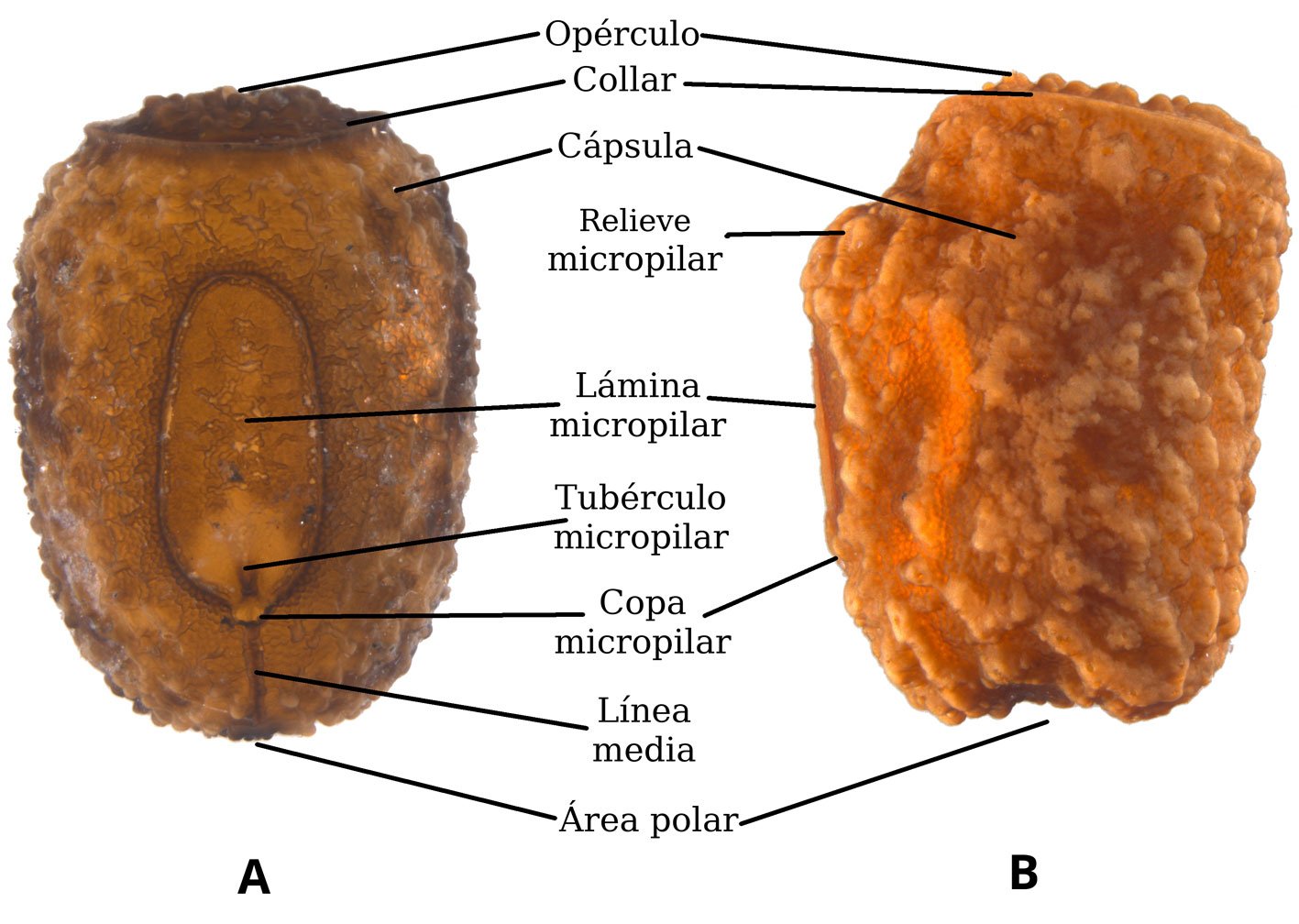
Tabla 4
Medidas en micras (μm) de cada huevo de P. phalangiphora utilizadas para el PCA.
| Clave | Medidas de huevo | ||||||
| L | W | H | mpl | mpw | oph | opw | |
| PphH1-1 | 2,774 | 1,752 | 1,971 | 876 | 474.5 | 1,423.5 | 1,131.5 |
| PphH1-2 | 2,737.5 | 1,752 | 1,898 | 912.5 | 474.5 | 1,350.5 | 1,058.5 |
| PphH1-3 | 2,664.5 | 1,533 | 1,788.5 | 912.5 | 511 | 1,350.5 | 1,095 |
| PphH1-4 | 2,701 | 1,715.5 | 1,898 | 876 | 474.5 | 1,460 | 1,131.5 |
| PphH1-5 | 2,628 | 1,679 | 1,861.5 | 949 | 511 | 1,460 | 1,095 |
| PphH1-6 | 2,847 | 1,715.5 | 1,898 | 766.5 | 511 | 1,460 | 1,204.5 |
| PphH1-7 | 2,737.5 | 1,679 | 1,861.5 | 766.5 | 511 | 1,496.5 | 1,095 |
| PphH1-8 | 2,847 | 1,788.5 | 1,861.5 | 912.5 | 438 | 1,423.5 | 1,168 |
| PphH1-9 | 2,774 | 1,642.5 | 1,861.5 | 803 | 511 | 1,460 | 1,204.5 |
| PphH1-10 | 2,774 | 1,679 | 1,861.5 | 876 | 547.5 | 1,350.5 | 1,095 |
| PphH1-11 | 2,810.5 | 1,679 | 1,934.5 | 839.5 | 438 | 1,460 | 1,168 |
| PphH1-12 | 2,847 | 1,752 | 1,861.5 | 803 | 474.5 | 1,460 | 1,168 |
| PphH1-13 | 2,737.5 | 1,715.5 | 1,861.5 | 766.5 | 474.5 | 1,460 | 1,131.5 |
| PphH1-14 | 2,664.5 | 1,642.5 | 1,861.5 | 839.5 | 474.5 | 1,387 | 1,058.5 |
| PphH1-15 | 2,920 | 1,788.5 | 1,934.5 | 912.5 | 511 | 1,496.5 | 1,168 |
| PphH2-1 | 2,372.5 | 1,387 | 1,496.5 | 839.5 | 474.5 | 1,350.5 | 1,058.5 |
| PphH2-2 | 2,555 | 1,679 | 1,752 | 803 | 438 | 1,715.5 | 1,387 |
| PphH2-3 | 2,555 | 1,569.5 | 1,642.5 | 912.5 | 438 | 1,533 | 1,314 |
| PphH2-4 | 2,591.5 | 1,898 | 1,861.5 | 766.5 | 438 | 1,752 | 1,387 |
| PphH2-5 | 2,555 | 1,606 | 1,825 | 766.5 | 401.5 | 1,606 | 1,277.5 |
| PphH2-6 | 2,591.5 | 1,606 | 1,825 | 766.5 | 438 | 1,642.5 | 1,387 |
| PphH2-7 | 2,664.5 | 1,642.5 | 1,825 | 766.5 | 438 | 1,642.5 | 1,387 |
| PphH2-8 | 2,555 | 1,679 | 1,861.5 | 803 | 438 | 1,642.5 | 1,277.5 |
| PphH2-9 | 2,591.5 | 1,642.5 | 1,825 | 949 | 547.5 | 1,606 | 1,241 |
| PphH2-10 | 2,628 | 1,642.5 | 1,788.5 | 693.5 | 438 | 1,533 | 1,314 |
| PphH2-11 | 2,628 | 1,496.5 | 1,679 | 839.5 | 511 | 1,460 | 1,168 |
| PphH2-12 | 2,591.5 | 1,606 | 1,752 | 839.5 | 438 | 1,606 | 1,314 |
| PphH2-13 | 2,591.5 | 1,496.5 | 1,715.5 | 839.5 | 401.5 | 1,460 | 1,277.5 |
| PphH2-14 | 2,591.5 | 1,679 | 1,788.5 | 730 | 438 | 1,423.5 | 1,350.5 |
| PphH2-15 | 2,664.5 | 1,715.5 | 2,007.5 | 912.5 | 438 | 1,715.5 | 1,423.5 |
| PphH3-1 | 2,774 | 1,642.5 | 1,898 | 803 | 474.5 | 1,387 | 1,095 |
| PphH3-2 | 2,664.5 | 1,642.5 | 1,825 | 803 | 474.5 | 1,387 | 1,095 |
| PphH3-3 | 2,664.5 | 1,642.5 | 1,788.5 | 839.5 | 511 | 1,314 | 1,058.5 |
| PphH3-4 | 2,737.5 | 1,642.5 | 1,825 | 766.5 | 547.5 | 1,387 | 1,095 |
| PphH3-5 | 2,628 | 1,679 | 1,788.5 | 803 | 511 | 1,350.5 | 1,058.5 |
| PphH3-6 | 2,737.5 | 1,642.5 | 1,788.5 | 803 | 511 | 1,314 | 1,095 |
| PphH3-7 | 2,774 | 1,642.5 | 1,825 | 803 | 511 | 1,387 | 1,095 |
| Tabla 4. Continúa | |||||||
| Clave | Medidas de huevo | ||||||
| L | W | H | mpl | mpw | oph | opw | |
| PphH3-8 | 2,737.5 | 1,679 | 1,825 | 876 | 511 | 1,460 | 1,095 |
| PphH3-9 | 2,701 | 1,679 | 1,861.5 | 803 | 547.5 | 1,350.5 | 1,022 |
| PphH3-10 | 2,701 | 1,642.5 | 1,788.5 | 766.5 | 438 | 1,350.5 | 1,095 |
| PphH3-11 | 2,701 | 1,606 | 1,898 | 839.5 | 547.5 | 1,496.5 | 1,131.5 |
| PphH3-12 | 2,701 | 1,642.5 | 1,861.5 | 876 | 547.5 | 1,496.5 | 1,095 |
| PphH3-13 | 2,664.5 | 1,606 | 1,825 | 839.5 | 438 | 1,350.5 | 1,204.5 |
| PphH3-14 | 2,737.5 | 1,642.5 | 1,752 | 803 | 474.5 | 1,350.5 | 1,095 |
| PphH3-15 | 2,774 | 1,679 | 1,788.5 | 876 | 438 | 1,168 | 1,058.5 |
Tabla 5
Medidas en μm de cada huevo de Pseudosermyle procera utilizadas para el PCA.
| Clave | Medidas de huevo | ||||||
| L | W | H | mpl | mpw | oph | opw | |
| PprP1-1 | 2,737.5 | 1,825 | 1,934.5 | 693.5 | 292 | 1,496.5 | 1,241 |
| PprP1-2 | 2,774 | 1,788.5 | 1,934.5 | 730 | 292 | 1,460 | 1,241 |
| PprP1-3 | 2,737.5 | 1,788.5 | 1,934.5 | 657 | 255.5 | 1,423.5 | 1,168 |
| PprP1-4 | 2,737.5 | 1,679 | 1,861.5 | 693.5 | 292 | 1,423.5 | 1,168 |
| PprP1-5 | 2,555 | 1,606 | 1,788.5 | 730 | 328.5 | 1,314 | 1,095 |
| PprP1-6 | 2,664.5 | 1,642.5 | 1,861.5 | 657 | 292 | 1,350.5 | 1,204.5 |
| PprP1-7 | 2,737.5 | 1,752 | 1,934.5 | 730 | 255.5 | 1,387 | 1,131.5 |
| PprP1-8 | 2,737.5 | 1,788.5 | 1,934.5 | 730 | 292 | 1,314 | 1,131.5 |
| PprP1-9 | 2,737.5 | 1,715.5 | 1,934.5 | 730 | 292 | 1,460 | 1,204.5 |
| PprP1-10 | 2,737.5 | 1,752 | 1,971 | 693.5 | 255.5 | 1,387 | 1,131.5 |
| PprP1-11 | 2,664.5 | 1,715.5 | 1,898 | 693.5 | 255.5 | 1,387 | 1,095 |
| PprP1-12 | 2,810.5 | 1,788.5 | 1,898 | 693.5 | 292 | 1,387 | 1,095 |
| PprP1-13 | 2,701 | 1,752 | 1,934.5 | 657 | 255.5 | 1,350.5 | 1,095 |
| PprP1-14 | 2,810.5 | 1,752 | 1,934.5 | 766.5 | 292 | 1,460 | 1,168 |
| PprP1-15 | 2,810.5 | 1,679 | 1,934.5 | 693.5 | 292 | 1,460 | 1,131.5 |
| PprP2-1 | 2,774 | 1,715.5 | 1,861.5 | 693.5 | 365 | 1,350.5 | 1,204.5 |
| PprP2-2 | 2,664.5 | 1,788.5 | 2,044 | 657 | 365 | 1,423.5 | 1,095 |
| PprP2-3 | 2,737.5 | 1,679 | 1,971 | 584 | 328.5 | 1,569.5 | 1,131.5 |
| PprP2-4 | 2,737.5 | 1,715.5 | 1,898 | 620.5 | 365 | 1,387 | 1,131.5 |
| PprP2-5 | 2,737.5 | 1,752 | 1,898 | 693.5 | 365 | 1,496.5 | 1,131.5 |
| PprP2-6 | 2,701 | 1,679 | 1,861.5 | 693.5 | 328.5 | 1,387 | 1,204.5 |
| PprP2-7 | 2,774 | 1,715.5 | 1,898 | 620.5 | 365 | 1,460 | 1,095 |
| PprP2-8 | 2,737.5 | 1,715.5 | 1,934.5 | 730 | 365 | 1,460 | 1,168 |
| Tabla 5. Continúa | |||||||
| Clave | Medidas de huevo | ||||||
| L | W | H | mpl | mpw | oph | opw | |
| PprP2-9 | 2,701 | 1,715.5 | 1,934.5 | 657 | 328.5 | 1,460 | 1,168 |
| PprP2-10 | 2,774 | 1,752 | 1,934.5 | 657 | 365 | 1,423.5 | 1,241 |
| PprP2-11 | 2,737.5 | 1,715.5 | 1,898 | 730 | 401.5 | 1,460 | 1,168 |
| PprP2-12 | 2,810.5 | 1,715.5 | 1,898 | 730 | 328.5 | 1,423.5 | 1,131.5 |
| PprP2-13 | 2,664.5 | 1,679 | 1,861.5 | 620.5 | 292 | 1,460 | 1,131.5 |
| PprP2-14 | 2,664.5 | 1,679 | 1,861.5 | 657 | 365 | 1,387 | 1,131.5 |
| PprP2-15 | 2,810.5 | 1,679 | 1,898 | 693.5 | 365 | 1,387 | 1,168 |
| PprP3-1 | 2,737.5 | 1,788.5 | 2,007.5 | 730 | 401.5 | 1,569.5 | 1,241 |
| PprP3-2 | 2,628 | 1,788.5 | 1,898 | 730 | 401.5 | 1,460 | 1,204.5 |
| PprP3-3 | 2,737.5 | 1,825 | 2,007.5 | 657 | 438 | 1,569.5 | 1,277.5 |
| PprP3-4 | 2,701 | 1,788.5 | 1,971 | 730 | 401.5 | 1,533 | 1,241 |
| PprP3-5 | 2,628 | 1,825 | 2,007.5 | 657 | 365 | 1,569.5 | 1,241 |
| PprP3-6 | 2,701 | 1,788.5 | 1,934.5 | 657 | 401.5 | 1,496.5 | 1,204.5 |
| PprP3-7 | 2,701 | 1,788.5 | 1,934.5 | 657 | 401.5 | 1,533 | 1,241 |
| PprP3-8 | 2,591.5 | 1,788.5 | 1,971 | 620.5 | 365 | 1,496.5 | 1,168 |
| PprP3-9 | 2,701 | 1,788.5 | 1,971 | 693.5 | 438 | 1,569.5 | 1,168 |
| PprP3-10 | 2,591.5 | 1,788.5 | 1,971 | 620.5 | 401.5 | 1,642.5 | 1,241 |
| PprP3-11 | 2,737.5 | 1,752 | 1,934.5 | 657 | 438 | 1,569.5 | 1,241 |
| PprP3-12 | 2,774 | 1,825 | 2,007.5 | 730 | 401.5 | 1,569.5 | 1,277.5 |
| PprP3-13 | 2,701 | 1,715.5 | 2,044 | 620.5 | 401.5 | 1,533 | 1,277.5 |
| PprP3-14 | 2,628 | 1,825 | 2,007.5 | 693.5 | 401.5 | 1,533 | 1,204.5 |
| PprP3-15 | 2,664.5 | 1,825 | 2,007.5 | 657 | 401.5 | 1,642.5 | 1,277.5 |
Tabla 6
Medidas en μm de cada huevo de Pseudosermyle striata utilizadas para el PCA.
| Clave | Medidas de huevo | ||||||
| L | W | H | mpl | mpw | oph | opw | |
| PstS1-1 | 2,263.8 | 1,470 | 1,675.8 | 1,234.8 | 529.2 | 1,029 | 882 |
| PstS1-2 | 2,352 | 1,587.6 | 1,734.6 | 1,234.8 | 529.2 | 1,146.6 | 1,029 |
| PstS1-3 | 2,293.2 | 1,528.8 | 1,705.2 | 1,205.4 | 529.2 | 1,087.8 | 940.8 |
| PstS1-4 | 2,352 | 1,558.2 | 1,646.4 | 1,205.4 | 529.2 | 1,087.8 | 1,029 |
| PstS1-5 | 2,116.8 | 1,528.8 | 1,705.2 | 1,058.4 | 529.2 | 1,176 | 999.6 |
| PstS1-6 | 2,175.6 | 1,499.4 | 1,705.2 | 1,087.8 | 588 | 1,117.2 | 970.2 |
| PstS1-7 | 2,234.4 | 1,470 | 1,646.4 | 1,117.2 | 558.6 | 1,146.6 | 970.2 |
| PstS1-8 | 2,263.8 | 1,528.8 | 1,646.4 | 1,058.4 | 558.6 | 1,176 | 1029 |
| Tabla 6. Continúa | |||||||
| Clave | Medidas de huevo | ||||||
| L | W | H | mpl | mpw | oph | opw | |
| PstS1-9 | 2,175.6 | 1,470 | 1,675.8 | 1,087.8 | 588 | 1,146.6 | 999.6 |
| PstS1-10 | 2,087.4 | 1,499.4 | 1,705.2 | 1,029 | 558.6 | 1,117.2 | 999.6 |
| PstS1-11 | 2,175.6 | 1,440.6 | 1,646.4 | 1,058.4 | 529.2 | 1,146.6 | 970.2 |
| PstS1-12 | 2,116.8 | 1,470 | 1,705.2 | 1,087.8 | 529.2 | 1,117.2 | 911.4 |
| PstS1-13 | 2,116.8 | 1,499.4 | 1,675.8 | 1,176 | 529.2 | 1,117.2 | 940.8 |
| PstS1-14 | 2,146.2 | 1,558.2 | 1,675.8 | 1,117.2 | 529.2 | 1,058.4 | 940.8 |
| PstS1-15 | 2,205 | 1,499.4 | 1,646.4 | 1,087.8 | 588 | 1,087.8 | 911.4 |
| PstS2-1 | 2,322.6 | 1,558.2 | 1,705.2 | 1,029 | 529.2 | 1,087.8 | 940.8 |
| PstS2-2 | 2,293.2 | 1,558.2 | 1,705.2 | 1,117.2 | 588 | 1,058.4 | 970.2 |
| PstS2-3 | 2,263.8 | 1,528.8 | 1,646.4 | 999.6 | 529.2 | 1,087.8 | 940.8 |
| PstS2-4 | 2,263.8 | 1,352.4 | 1,528.8 | 1,058.4 | 558.6 | 999.6 | 911.4 |
| PstS2-5 | 2,175.6 | 1,499.4 | 1,646.4 | 911.4 | 529.2 | 1,087.8 | 940.8 |
| PstS2-6 | 2,322.6 | 1,558.2 | 1,734.6 | 1,058.4 | 529.2 | 1,087.8 | 940.8 |
| PstS2-7 | 2,263.8 | 1,411.2 | 1,734.6 | 1,058.4 | 558.6 | 1,117.2 | 970.2 |
| PstS2-8 | 2,205 | 1,558.2 | 1,675.8 | 1,029 | 558.6 | 1,087.8 | 940.8 |
| PstS2-9 | 2,352 | 1,558.2 | 1,734.6 | 1,205.4 | 499.8 | 1,087.8 | 970.2 |
| PstS2-10 | 2,381.4 | 1,558.2 | 1,675.8 | 1,087.8 | 558.6 | 1,029 | 940.8 |
| PstS2-11 | 2,263.8 | 1,499.4 | 1,617 | 970.2 | 558.6 | 1,058.4 | 911.4 |
| PstS2-12 | 2,234.4 | 1,499.4 | 1,675.8 | 1,087.8 | 558.6 | 1,029 | 911.4 |
| PstS2-13 | 2,293.2 | 1,470 | 1,646.4 | 1,176 | 529.2 | 1,058.4 | 911.4 |
| PstS2-14 | 2,175.6 | 1,411.2 | 1,558.2 | 970.2 | 529.2 | 1,029 | 882 |
| PstS2-15 | 2,116.8 | 1,323 | 1,499.4 | 999.6 | 558.6 | 970.2 | 852.6 |
| PstS3-1 | 2,146.2 | 1,440.6 | 1,587.6 | 999.6 | 470.4 | 999.6 | 911.4 |
| PstS3-2 | 2,116.8 | 1,440.6 | 1,675.8 | 940.8 | 441 | 1,058.4 | 793.8 |
| PstS3-3 | 2,175.6 | 1,352.4 | 1,528.8 | 940.8 | 558.6 | 940.8 | 852.6 |
| PstS3-4 | 2,175.6 | 1,470 | 1,499.4 | 970.2 | 470.4 | 999.6 | 911.4 |
| PstS3-5 | 2,146.2 | 1,440.6 | 1,587.6 | 999.6 | 529.2 | 999.6 | 940.8 |
| PstS3-6 | 2,028.6 | 1,440.6 | 1,587.6 | 999.6 | 470.4 | 1,058.4 | 911.4 |
| PstS3-7 | 2,146.2 | 1,440.6 | 1,617 | 940.8 | 441 | 1,029 | 911.4 |
| PstS3-8 | 2,205 | 1,528.8 | 1,617 | 911.4 | 470.4 | 1,058.4 | 970.2 |
| PstS3-9 | 2,116.8 | 1,470 | 1,558.2 | 970.2 | 470.4 | 1,029 | 911.4 |
| PstS3-10 | 2,175.6 | 1,499.4 | 1,646.4 | 911.4 | 499.8 | 1,029 | 940.8 |
| PstS3-11 | 2,087.4 | 1,411.2 | 1,470 | 852.6 | 529.2 | 999.6 | 882 |
| PstS3-12 | 2,087.4 | 1,470 | 1,528.8 | 911.4 | 499.8 | 999.6 | 911.4 |
| PstS3-13 | 2,175.6 | 1,470 | 1,528.8 | 940.8 | 529.2 | 1,029 | 911.4 |
| PstS3-14 | 2,352 | 1,558.2 | 1,764 | 1,146.6 | 529.2 | 1,146.6 | 999.6 |
| PstS3-15 | 2,410.8 | 1,528.8 | 1,705.2 | 1,264.2 | 529.2 | 1,117.2 | 1,058.4 |
Tabla 7
Medidas en μm de cada huevo de Pseudosermyle carinulata, Pseudosermyle tridens, Pseudosermyle sp. 4, Pseudosermyle sp. 5 utilizadas para el PCA.
| Clave | Medidas de huevo | ||||||
| L | W | H | mpl | mpw | oph | opw | |
| PtrGtoU-1 | 3,580.2 | 1,285.2 | 1,514.7 | 642.6 | 596.7 | 872.1 | 688.5 |
| PtrGtoU-2 | 3,626.1 | 1,239.3 | 1,560.6 | 642.6 | 550.8 | 872.1 | 688.5 |
| PtrGtoU-3 | 3,626.1 | 1,377 | 1,606.5 | 642.6 | 596.7 | 872.1 | 688.5 |
| PtrGtoU-4 | 3,626.1 | 1,377 | 1,468.8 | 688.5 | 596.7 | 872.1 | 688.5 |
| PtrGtoU-5 | 3,580.2 | 1,285.2 | 1,560.6 | 734.4 | 550.8 | 826.2 | 734.4 |
| PtrGtoU-6 | 3,580.2 | 1,331.1 | 1,560.6 | 688.5 | 550.8 | 872.1 | 688.5 |
| PtrGtoU-7 | 3,672 | 1,331.1 | 1,514.7 | 688.5 | 596.7 | 826.2 | 734.4 |
| PtrGtoU-8 | 3,672 | 1,377 | 1,422.9 | 688.5 | 550.8 | 872.1 | 642.6 |
| PtrGtoU-9 | 3,672 | 1,377 | 1,514.7 | 688.5 | 550.8 | 872.1 | 688.5 |
| PtrGtoU-10 | 3,580.2 | 1,377 | 1,377 | 459 | 459 | 872.1 | 642.6 |
| PtrGtoU-11 | 3,580.2 | 1,285.2 | 1,422.9 | 321.3 | 229.5 | 872.1 | 688.5 |
| PtrGtoU-12 | 3,672 | 1,331.1 | 1,422.9 | 596.7 | 459 | 826.2 | 688.5 |
| PtrGtoU-13 | 3,580.2 | 1,239.3 | 1,422.9 | 688.5 | 550.8 | 872.1 | 734.4 |
| PtrGtoU-14 | 3,534.3 | 1,331.1 | 1,514.7 | 642.6 | 596.7 | 826.2 | 688.5 |
| PtrGtoU-15 | 3,488.4 | 1,331.1 | 1,606.5 | 688.5 | 596.7 | 872.1 | 734.4 |
| PtrMorT1-1 | 3,488.4 | 1,285.2 | 1,422.9 | 596.7 | 504.9 | 734.4 | 780.3 |
| PtrMorT1-2 | 3,626.1 | 1,331.1 | 1,514.7 | 504.9 | 504.9 | 734.4 | 780.3 |
| PtrMorT1-3 | 3,717.9 | 1,377 | 1,514.7 | 550.8 | 504.9 | 734.4 | 780.3 |
| PtrMorT1-4 | 3,580.2 | 1,331.1 | 1,468.8 | 504.9 | 504.9 | 780.3 | 780.3 |
| PtrMorT1-5 | 3,534.3 | 1,377 | 1,468.8 | 550.8 | 504.9 | 780.3 | 826.2 |
| PtrMorT1-6 | 3,672 | 1,331.1 | 1,468.8 | 550.8 | 504.9 | 734.4 | 780.3 |
| PtrMorT1-7 | 3,580.2 | 1,331.1 | 1,377 | 459 | 504.9 | 734.4 | 734.4 |
| PtrMorT1-8 | 3,580.2 | 1,377 | 1,377 | 596.7 | 504.9 | 642.6 | 734.4 |
| PtrMorT1-9 | 3,442.5 | 1,331.1 | 1,422.9 | 550.8 | 550.8 | 780.3 | 826.2 |
| PtrMorT1-10 | 3,442.5 | 1,239.3 | 1,377 | 550.8 | 550.8 | 780.3 | 826.2 |
| PtrMorT2-1 | 3,549.6 | 1,326 | 1,433.1 | 540.6 | 515.1 | 744.6 | 785.4 |
| PtrMorT2-2 | 3,488.4 | 1,239.3 | 1,422.9 | 688.5 | 550.8 | 734.4 | 780.3 |
| PtrMorT2-3 | 3,626.1 | 1,147.5 | 1,468.8 | 642.6 | 367.2 | 734.4 | 734.4 |
| PtrMorT2-4 | 3,442.5 | 1,147.5 | 1,331.1 | 688.5 | 550.8 | 734.4 | 780.3 |
| PtrMorT2-5 | 3,717.9 | 1,285.2 | 1,514.7 | 688.5 | 550.8 | 734.4 | 780.3 |
| PtrMorT2-6 | 3,717.9 | 1,239.3 | 1,468.8 | 688.5 | 550.8 | 734.4 | 734.4 |
| PtrMorT2-7 | 3,626.1 | 1,239.3 | 1,422.9 | 688.5 | 596.7 | 688.5 | 780.3 |
| PtrMorT2-8 | 3,717.9 | 1,285.2 | 1,468.8 | 642.6 | 550.8 | 826.2 | 780.3 |
| PtrMorT2-9 | 3,717.9 | 1,239.3 | 1,422.9 | 688.5 | 596.7 | 734.4 | 780.3 |
| PtrMorT2-10 | 3,672 | 1,193.4 | 1,514.7 | 642.6 | 596.7 | 734.4 | 780.3 |
| PcaC1-1 | 1,999.2 | 1,381.8 | 1,587.6 | 1,029 | 382.2 | 940.8 | 823.2 |
| Tabla 7. Continúa | |||||||
| Clave | Medidas de huevo | ||||||
| L | W | H | mpl | mpw | oph | opw | |
| PcaC1-2 | 1,999.2 | 1,411.2 | 1,587.6 | 999.6 | 382.2 | 970.2 | 823.2 |
| PcaC1-3 | 2,028.6 | 1,381.8 | 1,587.6 | 1,029 | 411.6 | 940.8 | 823.2 |
| PcaC1-4 | 2,058 | 1,352.4 | 1,558.2 | 940.8 | 382.2 | 940.8 | 852.6 |
| PcaC1-5 | 1,969.8 | 1,323 | 1,558.2 | 940.8 | 382.2 | 940.8 | 823.2 |
| PcaC2-1 | 1,852.2 | 1,176 | 1,381.8 | 940.8 | 441 | 823.2 | 735 |
| PcaC2-2 | 1,822.8 | 1,264.2 | 1,440.6 | 911.4 | 411.6 | 882 | 764.4 |
| PspFU-1 | 2,058 | 1,323 | 1,558.2 | 1,117.2 | 411.6 | 999.6 | 823.2 |
| PspFU-2 | 2,028.6 | 1,323 | 1,499.4 | 1,234.8 | 382.2 | 999.6 | 793.8 |
| PspFU-3 | 2,087.4 | 1,352.4 | 1,587.6 | 1,146.6 | 382.2 | 911.4 | 735 |
Tabla 8
Medidas en μm de cada huevo de N. isabelae, Pseudosermyle sp. 1, Pseudosermyle sp. 2. Pseudosermyle sp. 5 utilizadas para el PCA.
| Clave | Medidas de huevo | ||||||
| L | W | H | mpl | mpw | oph | opw | |
| PspFU-4 | 1,822.8 | 1,146.6 | 1,440.6 | 940.8 | 411.6 | 970.2 | 676.2 |
| PspFU-5 | 1,940.4 | 1,264.2 | 1,499.4 | 970.2 | 382.2 | 911.4 | 676.2 |
| PspFU-6 | 1,881.6 | 1,234.8 | 1,470 | 1,029 | 411.6 | 940.8 | 705.6 |
| PspFU-7 | 1,940.4 | 1,293.6 | 1,470 | 940.8 | 411.6 | 911.4 | 705.6 |
| PspFU-8 | 1,911 | 1,205.4 | 1,499.4 | 911.4 | 382.2 | 970.2 | 764.4 |
| PspFU-9 | 1,852.2 | 1,205.4 | 1,470 | 940.8 | 382.2 | 970.2 | 764.4 |
| PspFU-10 | 2,058 | 1,323 | 1,499.4 | 1,087.8 | 382.2 | 999.6 | 735 |
| PspFU-11 | 2,087.4 | 1,323 | 1,499.4 | 1,058.4 | 382.2 | 999.6 | 793.8 |
| PspFU-12 | 1,999.2 | 1,323 | 1,470 | 1,205.4 | 382.2 | 970.2 | 764.4 |
| PspFU-13 | 1,881.6 | 1,234.8 | 1,440.6 | 1,058.4 | 411.6 | 911.4 | 793.8 |
| PspFU-14 | 2,058 | 1,323 | 1,528.8 | 1,087.8 | 382.2 | 1,029 | 764.4 |
| PspFU-15 | 1,940.4 | 1,293.6 | 1,499.4 | 999.6 | 382.2 | 999.6 | 705.6 |
| NisaU-1 | 2,263.8 | 1,499.4 | 1,764 | 1,029 | 617.4 | 1,293.6 | 970.2 |
| NisaU-2 | 2,293.2 | 1,470 | 1,705.2 | 999.6 | 588 | 1,146.6 | 882 |
| NisaU-3 | 2,293.2 | 1,646.4 | 1,793.4 | 1,029 | 617.4 | 1,234.8 | 1,029 |
| NisaU-4 | 2,175.6 | 1,558.2 | 1,705.2 | 999.6 | 558.6 | 1,205.4 | 1,029 |
| NisaU-5 | 2,263.8 | 1,646.4 | 1,793.4 | 999.6 | 588 | 1,234.8 | 1,029 |
| NisaU-6 | 2,146.2 | 1,470 | 1,558.2 | 1,087.8 | 558.6 | 1,117.2 | 940.8 |
| NisaU-7 | 2,293.2 | 1,558.2 | 1,793.4 | 1,029 | 588 | 1,234.8 | 1,029 |
| NisaU-8 | 2,146.2 | 1,440.6 | 1,617 | 999.6 | 558.6 | 1,087.8 | 940.8 |
| NisaU-9 | 2,175.6 | 1,528.8 | 1,617 | 1,087.8 | 558.6 | 1,146.6 | 911.4 |
| NisaU-10 | 2,293.2 | 1,587.6 | 1,793.4 | 970.2 | 588 | 1,176 | 911.4 |
| Tabla 8. Continúa | |||||||
| Clave | Medidas de huevo | ||||||
| L | W | H | mpl | mpw | oph | opw | |
| NisaU-11 | 2,116.8 | 1,558.2 | 1,793.4 | 970.2 | 617.4 | 1,234.8 | 1,058.4 |
| NisaU-12 | 2,352 | 1,499.4 | 1,764 | 1,058.4 | 646.8 | 1,293.6 | 1,029 |
| PtgVBU-1 | 3,394.5 | 1,569.5 | 1,715.5 | 1,533 | 657 | 1,277.5 | 912.5 |
| PtgVBU-2 | 3,029.5 | 1,350.5 | 1,606 | 1,350.5 | 511 | 912.5 | 620.5 |
| PtgVBU-3 | 3,467.5 | 1,533 | 1,752 | 1,496.5 | 730 | 1,204.5 | 803 |
| PtgVBU-4 | 3,394.5 | 1,533 | 1,606 | 1,496.5 | 657 | 1,095 | 803 |
| PtgVBU-5 | 3,321.5 | 1,496.5 | 1,642.5 | 1,533 | 620.5 | 1,204.5 | 912.5 |
| PtgVBU-6 | 3,431 | 1,460 | 1,642.5 | 1,460 | 584 | 1,095 | 803 |
| PtgVBU-7 | 3,431 | 1,460 | 1,642.5 | 1,460 | 657 | 1,241 | 839.5 |
| PtgVBU-8 | 3,394.5 | 1,533 | 1,569.5 | 1,533 | 693.5 | 1,095 | 839.5 |
| PtgVBU-9 | 3,467.5 | 1,533 | 1,715.5 | 1,460 | 620.5 | 1,095 | 766.5 |
| PtgVBU-10 | 3,394.5 | 1,533 | 1,715.5 | 1,496.5 | 730 | 1,168 | 912.5 |
| PtgVBU-11 | 3,285 | 1,606 | 1,679 | 1,460 | 620.5 | 1,204.5 | 876 |
| PtgDFG1-1 | 3,321.5 | 1,533 | 1,715.5 | 1,095 | 730 | 985.5 | 766.5 |
| PtgDFG1-2 | 3,102.5 | 1,533 | 1,606 | 1,131.5 | 693.5 | 839.5 | 693.5 |
| PtgDFG1-3 | 3,285 | 1,533 | 1,642.5 | 1,204.5 | 730 | 912.5 | 766.5 |
| PtgDFG1-4 | 3,102.5 | 1,460 | 1,533 | 1,204.5 | 693.5 | 949 | 766.5 |
| PtgDFG1-5 | 3,248.5 | 1,569.5 | 1,569.5 | 1,168 | 766.5 | 803 | 657 |
| PtgDFG2-1 | 3,248.5 | 1,533 | 1,642.5 | 1,241 | 657 | 949 | 620.5 |
| PtgDFG2-2 | 3,285 | 1,496.5 | 1,606 | 1,095 | 620.5 | 949 | 730 |
| PtgDFG2-3 | 3,248.5 | 1,496.5 | 1,569.5 | 1,350.5 | 730 | 949 | 803 |
| PtgDFG2-4 | 3,285 | 1,606 | 1,715.5 | 1,314 | 876 | 912.5 | 730 |
| PtgDFG2-5 | 3,102.5 | 1,606 | 1,752 | 1,241 | 876 | 949 | 730 |
Tabla 9
Medidas en μm de cada huevo de Pseudosermyle sp. 2. Pseudosermyle sp. 3, Pseudosermyle sp. 6 utilizadas para el PCA.
| Clave | Medidas de huevo | ||||||
| L | W | H | mpl | mpw | oph | opw | |
| PtgDFG2-6 | 3,285 | 1,496.5 | 1,606 | 1,314 | 620.5 | 912.5 | 657 |
| PtgDFG2-7 | 3,212 | 1,460 | 1,569.5 | 1,277.5 | 620.5 | 912.5 | 657 |
| PtgDFG2-8 | 3,321.5 | 1,533 | 1,679 | 1,277.5 | 657 | 985.5 | 693.5 |
| PtgDFG2-9 | 3,212 | 1,569.5 | 1,679 | 1,314 | 876 | 912.5 | 766.5 |
| PtgDFG2-10 | 3,175.5 | 1,606 | 1,752 | 1,387 | 657 | 876 | 657 |
| PtgDFG2-11 | 3,467.5 | 1,606 | 1,715.5 | 1,241 | 657 | 949 | 657 |
| PtgDFG2-12 | 3,248.5 | 1,606 | 1,642.5 | 1,277.5 | 693.5 | 985.5 | 839.5 |
| PtgDFG2-13 | 3,248.5 | 1,606 | 1,642.5 | 1,241 | 693.5 | 985.5 | 657 |
| Tabla 9. Continúa | |||||||
| Clave | Medidas de huevo | ||||||
| L | W | H | mpl | mpw | oph | opw | |
| PtgDFG2-14 | 3,285 | 1,496.5 | 1,642.5 | 1,460 | 730 | 949 | 803 |
| PchF1-1 | 3,626.1 | 1,147.5 | 1,422.9 | 1,239.3 | 688.5 | 918 | 780.3 |
| PchF1-2 | 3,993.3 | 1,468.8 | 1,652.4 | 1,422.9 | 734.4 | 1,055.7 | 826.2 |
| PchF1-3 | 3,947.4 | 1,514.7 | 1,606.5 | 1,468.8 | 826.2 | 1,101.6 | 872.1 |
| PchF2-1 | 3,947.4 | 1,377 | 1,698.3 | 1,377 | 688.5 | 918 | 780.3 |
| PchF2-2 | 3,672 | 1,377 | 1,560.6 | 1,377 | 780.3 | 872.1 | 688.5 |
| PchF2-3 | 3,672 | 1,422.9 | 1,606.5 | 1,422.9 | 780.3 | 872.1 | 688.5 |
| PoaxU-1 | 2,701 | 1,642.5 | 1,898 | 693.5 | 328.5 | 1,314 | 1,131.5 |
| PoaxU-2 | 2,518.5 | 1,569.5 | 1,825 | 693.5 | 365 | 1,277.5 | 1,095 |
| PoaxU-3 | 2,664.5 | 1,642.5 | 1,861.5 | 657 | 328.5 | 1,277.5 | 1,058.5 |
| PoaxU-4 | 2,664.5 | 1,679 | 1,825 | 657 | 365 | 1,277.5 | 1,131.5 |
| PoaxU-5 | 2,664.5 | 1,642.5 | 1,861.5 | 730 | 365 | 1,277.5 | 1,131.5 |
| PoaxU-6 | 2,518.5 | 1,606 | 1,788.5 | 693.5 | 365 | 1,241 | 1,095 |
| PoaxU-7 | 2,555 | 1,606 | 1,861.5 | 657 | 365 | 1,350.5 | 1,131.5 |
| PoaxU-8 | 2,591.5 | 1,642.5 | 1,861.5 | 766.5 | 328.5 | 1,277.5 | 1,131.5 |
| PoaxU-9 | 2,482 | 1,569.5 | 1,752 | 657 | 365 | 1,168 | 949 |
| PoaxU-10 | 2,591.5 | 1,569.5 | 1,861.5 | 657 | 365 | 1,241 | 1,095 |
| PoaxU-11 | 2,482 | 1,679 | 1,788.5 | 693.5 | 365 | 1,277.5 | 1,058.5 |
| PoaxU-12 | 2,518.5 | 1,569.5 | 1,788.5 | 693.5 | 328.5 | 1,277.5 | 1,095 |
| PoaxU-13 | 2,555 | 1,606 | 1,861.5 | 693.5 | 328.5 | 1,241 | 1,022 |
| PoaxU-14 | 2,555 | 1,679 | 1,788.5 | 693.5 | 365 | 1,241 | 1,022 |
| PoaxU-15 | 2,701 | 1,679 | 1,898 | 657 | 292 | 1,314 | 1,131.5 |
Se llevó a cabo un análisis de componentes principales (PCA) para examinar si las medidas —en micras— de los huevos eran relevantes al reconocer grupos. Las medidas utilizadas fueron: longitud de la cápsula (L), amplitud de la cápsula (W), altitud de la cápsula (H), longitud de la lámina micropilar (mpl), amplitud de la lámina micropilar (mpw), altitud del opérculo (oph) y amplitud del opérculo (opw) (tablas 4-9). Se incluyeron todos los huevos con el propósito de graficar estas mediciones y agruparlos según dichas medidas. Se empleó R (R Core Team, 2013) mediante la interfaz de Rstudio (Rstudio Team, 2015); las paqueterías utilizadas fueron: ggplot2 (Wickham, 2016), ggfortify (Horikoshi y Tang, 2016), rgl (Adler et al., 2018), pca3d (Weiner, 2017) y magick (Ooms, 2018). Cada huevo fue caracterizado de manera individual siguiendo un código que incluye los nombres de las columnas: nombre, clave de hembra de la tabla 3, más el número ascendente correspondiente (tablas 4-9). Para la descripción de los grupos, las medidas se convirtieron a milímetros (mm), mientras que para cada especie se mantuvieron en micras (μm).
Resultados
El análisis de componentes principales (PCA) muestra la formación de 4 grupos (fig. 3) explicados en detalle posteriormente, que coinciden con los patrones de morfología externa mostrada por los adultos (machos y hembras) y el tipo de oviposición. En el gráfico del PCA cada eje representa un componente; por lo tanto, se representan 2 gráficos del PCA, uno con rotación en el eje del primer componente (fig. 3A) y otro con rotación en el eje del segundo componente (fig. 3B), para una apreciación mejor de los 4 grupos. Los primeros 3 componentes explican 96.76% de la varianza (fig. 4A). El primer componente presenta mayor contribución de L (fig. 4B), mientras que el segundo presenta mayor homogeneidad en la contribución que recibe de las variables; sin embargo, la oph es la variable que más contribuye (fig. 4C). Finalmente, el tercer componente presenta mayor contribución de mpl (fig. 4D).
A continuación, se da una descripción breve de la microestructura coriónica general de cada grupo, así como para cada una de las especies incluidas en este trabajo. También se incluye una comparación de las distintas estructuras coriónicas entre los grupos y las especies, como se observa en las tablas 10-12. Muchas de estas especies no están descritas y pueden representar especies aún inéditas e innominadas, en consecuencia, se dejaron como morfoespecies y solo se enumeraron.
Tabla 10
Comparación entre estructuras coriónicas entre especies y grupos. Longitud de cápsula (L), amplitud de cápsula (W), altitud de cápsula (H).
| Grupos | General | Cápsula | ||||||
| Tipo de huevo | Oviposición | Forma | Textura | Microestructura | L promedio (mm) | W promedio (mm) | H promedio (mm) | |
| Grupo 1 | adhesivo | Adheridos | Fusiforme | Gránulos | Basamentos piramidales | 3.37 ±0.23 | 1.5 ±0.09 | 1.64 ±0.07 |
| Pseudosermyle sp. 1 | adhesivo | Adheridos | Fusiforme | Gránulos | Basamentos piramidales | 3.36 ±0.12 | 1.5 ±0.06 | 1.66 ±0.05 |
| Pseudosermyle sp. 2 | adhesivo | Adheridos | Fusiforme | Gránulos | Basamentos piramidales | 3.24 ±0.08 | 1.54 ±0.05 | 1.64 ±0.06 |
| Pseudosermyle sp. 3 | adhesivo | Adheridos | Fusiforme | Gránulos | Basamentos piramidales | 3.8 ±0.16 | 1.38 ±0.12 | 1.59 ±0.09 |
| Grupo 2 | adhesivo | Ooteca | Fusiforme | Paralelepípedos | Liso | 3.6 ±0.08 | 1.3 ±0.06 | 1.46 ±0.06 |
| Pseudosermyle tridens | adhesivo | Ooteca | Fusiforme | Paralelepípedos | Liso | 3.59 ±0.09 | 1.28 ±0.07 | 1.44 ±0.05 |
| Pseudosermyle sp. 4 | Adhesivo | Ooteca | Fusiforme | Paralelepípedos | Liso | 3.6 ±0.05 | 1.32 ±0.04 | 1.49 ±0.07 |
| Grupo 3 | Alveolada | Por caída | Doliforme | Variable | Variable | 2.14 ±0.14 | 1.44 ±0.11 | 1.61 ±0.1 |
| Pseudosermyle carinulata | Alveolada | Por caída | Doliforme | Gránulos | Proyecciones digitiformes | 1.96 ±0.08 | 1.32 ±0.08 | 1.52 ±0.08 |
| Pseudosermyle striata | Alveolada | Por caída | Doliforme | Arrugas | Proyecciones digitiformes | 2.21 ±0.09 | 1.48 ±0.06 | 1.64 ±0.07 |
| Pseudosermyle sp. 5 | Alveolada | Por caída | Doliforme | Arrugas | Rugulosa | 1.96 ±0.08 | 1.27 ±0.05 | 1.49 ±0.03 |
| Nooxapty isabelae | Alveolada | Por caída | Doliforme | Espinas | Proyecciones digitiformes | 2.23 ±0.07 | 1.53 ±0.06 | 1.72 ±0.08 |
| Grupo 4 | Alveolada | Por caída | Doliforme | Variable | Variable | 2.68 ±0.09 | 1.69 ±0.08 | 1.87 ±0.08 |
| Pseudosermyle phalangiphora | Alveolada | Por caída | Doliforme | Gibas con espinas umbeliformes | Punteada | 2.68 ±0.1 | 1.65 ±0.08 | 1.82 ±0.08 |
| Pseudosermyle procera | Alveolada | Por caída | Doliforme | Verrugosa con fóveas | Verrugosa | 2.71 ±0.06 | 1.74 ±0.05 | 1.93 ±0.05 |
| Pseudosermyle sp. 6 | Alveolar | Por caída | Doliforme | Coliculada con espinas umbeliformes | Verrugosa | 2.58 ±0.07 | 1.62 ±0.04 | 1.83 ±0.04 |
Tabla 11
Comparación entre estructuras coriónicas entre especies y grupos. Porcentaje de cobertura de la longitud de lámina micropilar en la longitud de la cápsula (% de mpl/L).
| Grupos | Opérculo | Lámina micropilar (mp) | ||||||
| Ornamentación | Ángulo opercular | Capas | Forma | Ornamentación | % de mpl/L | Relieve micropilar | Forma lámina micropilar interna | |
| Grupo 1 | Variable | + 55° | 1 | Lemniscata | Similar a la cápsula | 40 | Variable | Abierta con línea media |
| Pseudosermyle sp. 1 | Estructura solitaria | + 55° | 1 | Lemniscata | Similar a la cápsula | 43.98 | Presen-te | Abierta con línea media |
| Pseudosermyle sp. 2 | Similar a la cápsula | + 55° | 1 | Lemniscata | Similar a la cápsula | 38.63 | Ausente | Abierta con línea media |
| Pseudosermyle sp. 3 | Disposición radial | + 55° | 1 | Lemniscata | Similar a la cápsula | 36.34 | Presen-te | Abierta con línea media |
| Grupo 2 | Similar a la cápsula | + 40° | 2 | Variable | Distinta a la cápsula | 17 | Ausente | Paralela sin línea media |
| Pseudosermyle tridens | Similar a la cápsula | + 40° | 2 | Triangular | Distinta a la cápsula | 16.7 | Ausente | Paralela sin línea media |
| Pseudosermyle sp. 4 | Similar a la cápsula | + 40° | 2 | Circular | Distinta a la cápsula | 17.57 | Ausente | Paralela sin línea media |
| Grupo 3 | Similar a la cápsula | ≈ 0° | 1 | Oblonga | Similar a la cápsula | 50 | Ausente | Abierta con línea media |
| Pseudosermyle carinulata | Similar a la cápsula | ≈ 0° | 1 | Oblonga | Similar a la cápsula | 49.46 | Ausente | Abierta con línea media |
| Pseudosermyle striata | Similar a la cápsula | ≈ 0° | 1 | Oblonga | Similar a la cápsula | 47.51 | Ausente | Abierta con línea media |
| Pseudosermyle sp. 5 | Similar a la cápsula | ≈ 0° | 1 | Oblonga | Similar a la cápsula | 53.23 | Ausente | Abierta con línea media |
| Nooxapty isabelae | Similar a la cápsula | ≈ 0° | 1 | Oblonga | Similar a la cápsula | 45.72 | Ausente | Abierta con línea media |
| Grupo 4 | Acomodo de estructuras | ≈ 0° | 1 | Variable | Variable | 30 | Varia-ble | Abierta con línea media |
| Pseudosermyle phalangiphora | Estructura solitaria | ≈ 0° | 1 | Oblonga | Distinta a la cápsula | 30.885 | Ausente | Abierta con línea media |
| Pseudosermyle procera | Anillo | ≈ 0° | 1 | Elíptica | Distinta a la cápsula | 25.11 | Presen-te | Abierta con línea media |
| Pseudosermyle sp. 6 | Anillo | ≈ 0° | 1 | Oblonga | Similar a la cápsula | 26.55 | Ausente | Abierta con línea media |
Tabla 12
Comparación entre estructuras coriónicas entre especies y grupos. Lámina micropilar (mp).
| Grupos | Borde | Tubérculo micropilar | Copa micropilar | Línea media externa | |||
| Forma | Posición | Forma | Posición | Presencia | Ornamentación | Longitud | |
| Grupo 1 | Carina que se ensancha hacia la parte posterior | Hacia la copa micropilar | Variable | Fusionada al borde de mp | Presente | Variable | Corta (no llega al área polar) |
| Pseudosermyle sp. 1 | Carina que se ensancha hacia la parte posterior | Hacia la copa micropilar | Triángulo invertido | Fusionada al borde de mp | Presente | Carina | Corta (no llega al área polar) |
| Pseudosermyle sp. 2 | Carina que se ensancha hacia la parte posterior | Hacia la copa micropilar | Triángulo invertido | Fusionada al borde de mp | Presente | Cambio de textura | Corta (no llega al área polar) |
| Pseudosermyle sp. 3 | Carina que se ensancha hacia la parte posterior | Hacia la copa micropilar | Matraz invertido | Fusionada al borde de mp | Presente | Sucesión de estructuras | Corta (no llega al área polar) |
| Grupo 2 | Variable | En la mitad de la copa micropilar | Carina | Ausente | Ausente | No aplica | No aplica |
| Pseudosermyle tridens | Cambio de textura | En la mitad de la copa micropilar | Carina | Ausente | Ausente | No aplica | No aplica |
| Pseudosermyle sp. 4 | Ligera elevación | En la mitad de la copa micropilar | Carina | Ausente | Ausente | No aplica | No aplica |
| Grupo 3 | Variable | Hacia la copa micropilar | Variable | Separada del borde de mp | Presente | Variable | Variable |
| Pseudosermyle carinulata | Surco | Hacia la copa micropilar | Rectangular | Separada del borde de mp | Presente | Carina | Larga (llega al área polar) |
| Pseudosermyle striata | Carina | Hacia la copa micropilar | Triángulo invertido | Separada del borde de mp | Presente | Carina | Larga (llega al centro del área polar) |
| Pseudosermyle sp. 5 | Superficie lisa | Hacia la copa micropilar | Rectangular | Separada del borde de mp | Presente | Carina | Larga (llega al área polar) |
| Nooxapty isabelae | Carina | Hacia la copa micropilar | Forma de y | Separada del borde de mp | Presente | Sucesión de estructuras | Larga (llega al centro del área polar) |
| Grupo 4 | Carina | Hacia la copa micropilar | Variable | Fusionada al borde de mp | Variable | Variable | Variable |
| Tabla 12. Continúa | |||||||
| Grupos | Borde | Tubérculo micropilar | Copa micropilar | Línea media externa | |||
| Forma | Posición | Forma | Posición | Presencia | Ornamentación | Longitud | |
| Pseudosermyle phalangiphora | Carina | Hacia la copa micropilar | Semiesfera | Fusionada al borde de mp | Presente | Carina | Larga (llega al área polar) |
| Pseudosermyle procera | Carina | Hacia la copa micropilar | Semiesfera | Fusionada al borde de mp | Ausente | No aplica | No aplica |
| Pseudosermyle sp. 6 | Carina | Hacia la copa micropilar | Triángulo invertido | Fusionada al borde de mp | Presente | Sucesión de estructuras | Larga (llega al área polar) |
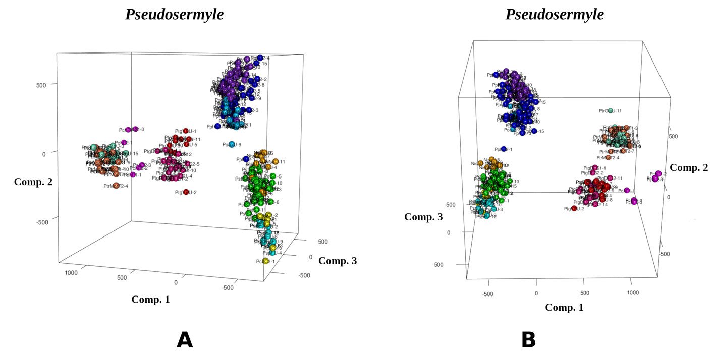
Pseudosermyle grupo 1
Huevo: adhesivo, adherido individualmente sobre una superficie (fig. 5B). Medidas en mm (n = 36): L = 3.37 ± 0.23 (3.02-3.99), W = 1.5 ± 0.09 (1.14-1.6), H = 1.64 ± 0.07 (1.42-1.75), mpl = 1.34 ± 0.12 (1.09-1.53), mpw = 0.69 ± 0.08 (0.51-0.87), oph = 0.99 ± 0.12 (0.8-1.27) y opw = 0.76 ± 0.08 (0.62-0.91). Opérculo orientado en + 55° aproximadamente. Lámina micropilar en forma de lemniscata u oblonga con el centro constreñido; con una longitud aproximada entre más de un tercio y menos de la mitad de la longitud de la cápsula. Lámina micropilar interna abierta con línea media (fig. 6A-C).
Especies incluidas: Pseudosermyle sp. 1, Pseudo-
sermyle sp. 2 y Pseudosermyle sp. 3.
Pseudosermyle sp. 1 (figs. 1, 6A, 7A, 8, 9)
Material examinado: 11 huevos. México. Edo. de México, Valle de Bravo, Arriba cueva, 19°5’32.928” N, 100°4’19.848” O, 2,260 m snm [voucher: PHMX 349-358 depositados en CNIN y MZFC].
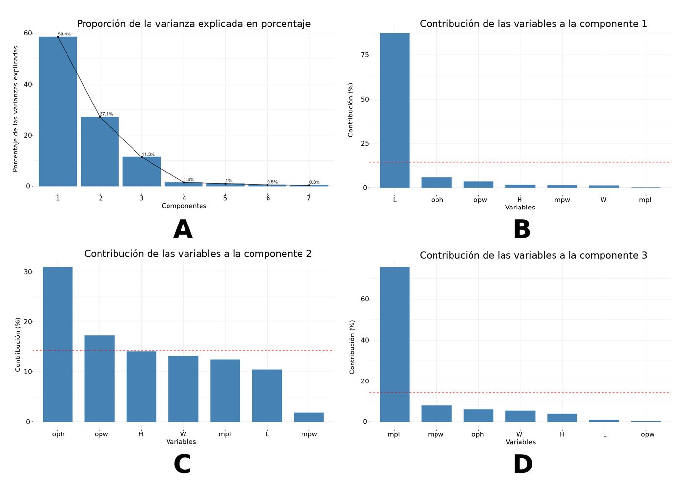
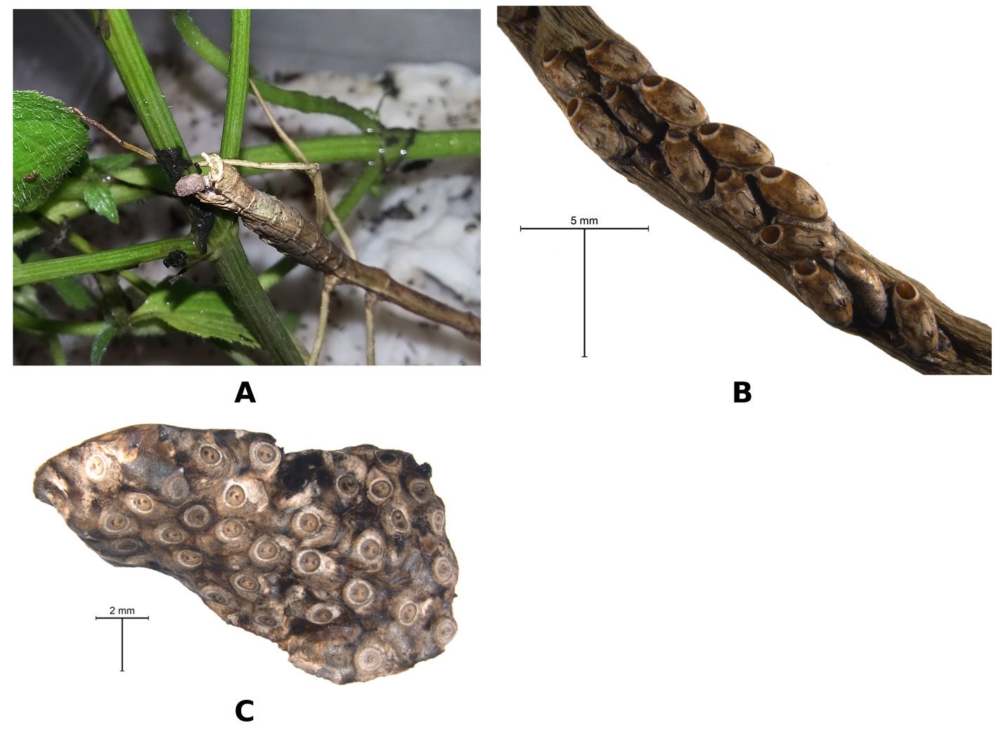
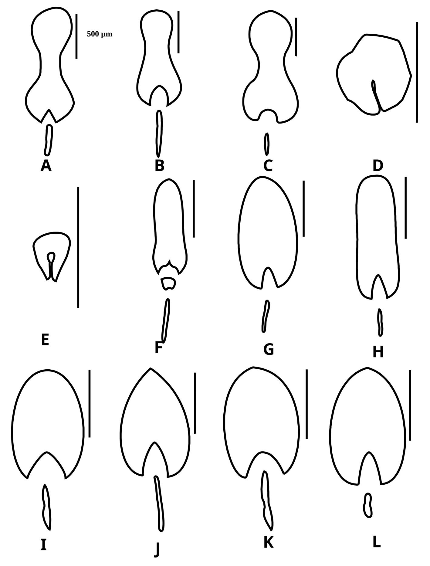
Medidas en μm: (n = 11) L= 3364.63 ± 124.11 (3029.5-3467.5), W = 1509.77 ± 67.84 (1350.5-1606), H = 1662.4 ± 57.39 (1569.5-1752), mpl = 1479.9 ± 52.54 (1350.5-1533), mpw = 643.72 ± 63.79 (511-730), oph = 1144.77 ± 100.98 (912.5-1277.5), opw = 826.22 ± 85.24 (620.5-912.5), %h/l (elongación) = 49.44 ± 1.97 (46.23-53.01), %w/h (compresión) = 90.86 ± 4 (84.09-97.67).
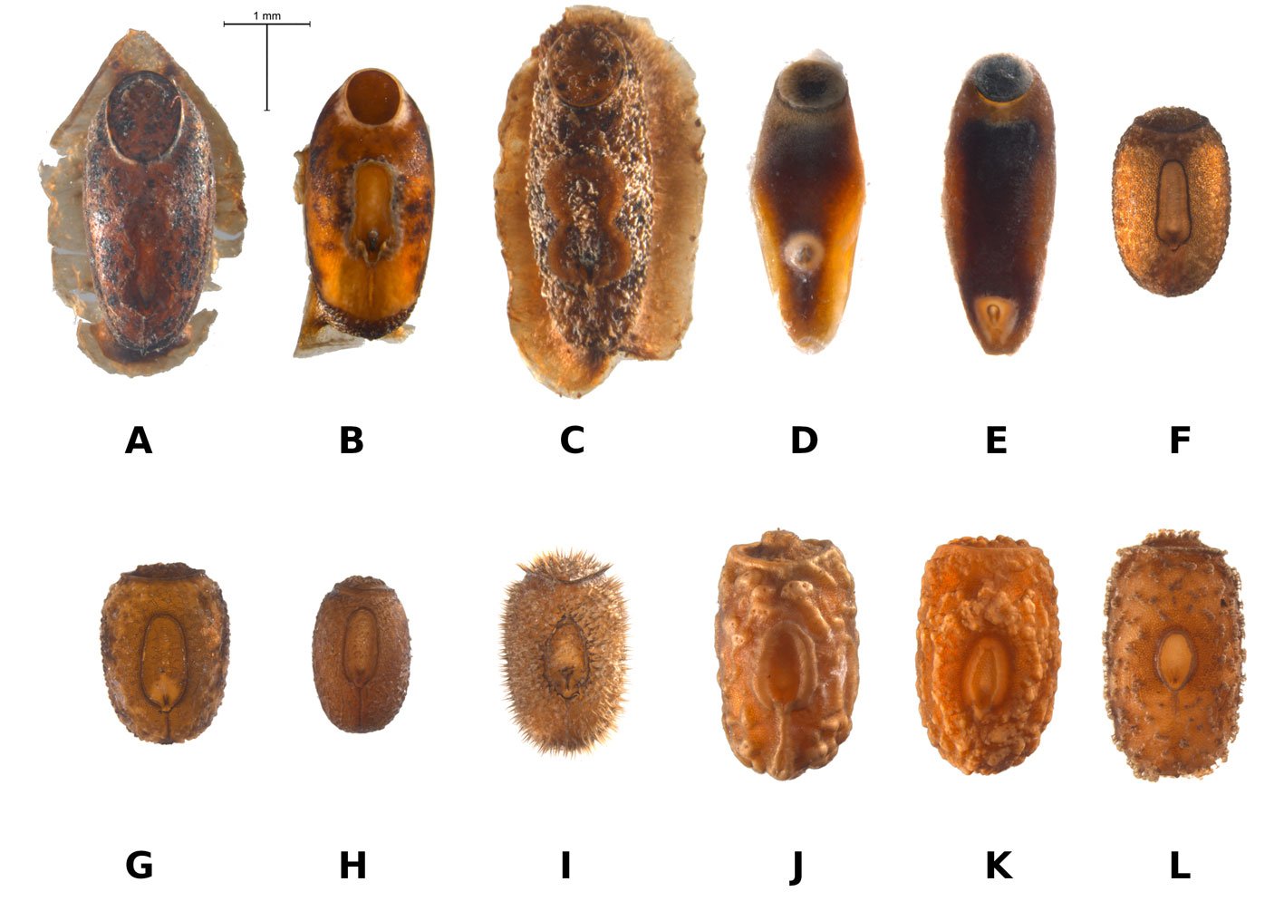
Microestructura: (n = 1) (figs. 8, 9) cápsula de superficie granulosa (fig. 8A, B), con granos formados por basamentos piramidales de 6-8 niveles (fig. 8E, F); la longitud varía entre 37.18-59.04 μm. En toda la superficie se observa un patrón de terrazas (polígonos irregulares y escalonados, en su mayoría rectangulares), que pueden o no formar los gránulos (fig. 8E). El huevo suele estar cubierto (cuando es ovipuesto) por una sustancia adherente o pegajosa que presenta rugosidades irregulares y separadas, suele cubrir la mitad ventral (fig. 8C, D); las arrugas son lisas (fig. 8D). Lámina micropilar con ornamentación y textura similar a la cápsula (fig. 9A). Borde a manera de una carina con 66 μm de amplitud (fig. 9D), tiende a ensancharse hacia la copa micropilar (fig. 9C). Tubérculo micropilar como un triángulo invertido, con 286 μm de longitud y 198 μm de amplitud (fig. 9C). Copa micropilar con forma de ‘y’, fusionada al borde, con 362 μm de amplitud y 39 μm de grosor (fig. 9C). Línea media como una carina de 40 μm de amplitud (figs. 8C, 9B). Las estructuras antes mencionadas, salvo la superficie de la lámina micropilar (fig. 9E), son de textura rugosa. Opérculo de superficie rugosa, con arrugas que forman una elevación a manera de semicírculo en la región anterior; la textura de las arrugas es verrugosa (fig. 9F).
Pseudosermyle sp. 2 (figs. 1, 6B, 7B, 10, 11)
Material examinado:19 huevos. México, Ciudad de México, Coyoacán, REPSA, Espacio Escultórico-Caseta de vigilancia, 19°19’3.4824” N, 99°11’5.4744” O, 2,311 m snm [voucher: PHMX 304-322 depositados en CNIN y MZFC].
Medidas en μm: (n = 19)L = 3246.57 ± 87.28 (3102.5-3467.5), W = 1544.52 ± 51.69 (1460-1606), H = 1646.34 ± 64.25 (1533-1752), mpl = 1254.44 ± 94.4 (1095-1460), mpw = 714.63 ± 82.8 (620.5-876), oph = 929.78 ± 49.22 (803-985.5), opw = 718.47 ± 63.28 (620.5-839.5), %h/l (elongación) = 50.73 ± 2.18 (48.31-56.47), %w/h (compresión) = 93.86 ± 2.59 (89.36-100).
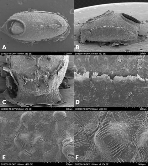
Microestructura: (n = 1) (figs. 10, 11) cápsula de superficie coliculado-granulosa (fig. 10A, B), con granos formados por basamentos piramidales de 4-6 niveles; la longitud varía entre 24.66-34.39 μm (fig. 10E, F). En toda la superficie se presenta un patrón de polígonos irregulares y escalonados —en su mayoría rectangulares, que pueden o no formar los gránulos (fig. 10E); en ciertas regiones hay máculas irregulares de textura escabriculosa. El huevo suele estar cubierto (cuando es ovipuesto) por una sustancia pegajosa que muestra rugosidades irregulares y muy cercanas entre sí, suele cubrir la mitad ventral (fig. 10B, C); las arrugas son lisas (fig. 10D). Lámina micropilar con ornamentación similar al patrón presente en la superficie de la cápsula (fig. 11A), con secciones irregulares de textura escabriculosa (fig. 11E). Borde como una carina de 73 μm de amplitudl (fig. 11D) y tiende a ensancharse hacia la copa micropilar (fig. 11C), con textura papilada (fig. 11D). Tubérculo micropilar como un triángulo invertido, con 282 μm de longitud y 136 μm de amplitud (fig. 11C); textura similar a la presente en la superficie de la cápsula (fig. 11C). Copa micropilar con forma de ‘v’, fusionada al borde, con 321 μm de amplitud y 45 μm de grosor, de superficie rugosa (fig. 11A, C). Línea media con 533 μm de longitud y 61 μm de amplitud (figs. 10C, 11B); de textura tuberculosa al centro y escabriculosa en la unión con la cápsula (fig. 11B) – esta línea media exhibe un cambio de texturas en la cápsula. Opérculo de textura rugulosa que forma secciones poligonales de grupos de protuberancias (fig. 11F).
Pseudosermyle sp. 3 (figs. 1, 6C, 7C, 12, 13)
Material examinado: 6 huevos. México, Jalisco, La Huerta, alrededores EB Chamela, 19°29’57.516” N, 105°2’41.424” O, 87 m snm [voucher: PHMX 323-328 depositados en CNIN y MZFC].
Medidas en μm: (n = 6) L = 3809.7 ± 169.27 (3626.1-3993.3), W = 1384.65 ±127.91 (1147.5-1514.7), H = 1591.2 ± 94.81 (1422.9-1689.3), mpl = 1384.65 ± 79.05 (1239.3-1468.8), mpw = 749.7 ± 55.58 (688.5-826.2), oph = 956.25 ± 98.08 (872.1-1101.6), opw = 772.65 ± 73.53 (688.5-872.1), %h/l (elongación) = 41.76 ± 1.65 (39.24-,43.75) y %w/h (compresión) = 86.95 ± 5.21 (80.64-94.28).
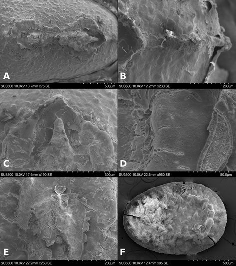
Microestructura: (n = 1) (figs. 12, 13) cápsula de superficie rugosa, con arrugas irregulares de longitud 54.04-148.04 μm y amplitud de 28.19-53.26 μm (fig. 12A, B); unidas por una especie de membrana (fig. 12D). Los espacios entre las arrugas están saturados de gránulos con diámetro 28.19-42.29 μm (fig. 12D, F), éstos suelen estar muy juntos hacia el dorso y más separados hacia los lados; en las superficies laterales se ven algunos niveles, como si fuesen basamentos piramidales (fig. 12E). El huevo suele estar cubierto (cuando ovipuesto) por una sustancia adherente que exhibe rugosidades irregulares y muy cercanas, suele cubrir la mitad ventral (fig. 12B, C); las arrugas son lisas (fig. 12D). Lámina micropilar con ornamentación y textura similar a la cápsula, salvo que las arrugas están hacia el centro (fig. 13E) y los gránulos hacia la periferia (fig. 13A).
Borde de textura escabriculosa elevada a manera de carina, con 77 μm de amplitud (fig. 13D). Tubérculo micropilar en forma de matraz invertido con 381 μm de longitud y 237 μm de amplitud, de textura rugosa (fig. 13C). Copa micropilar con forma de ‘v’, fusionada al borde, con 437 μm de amplitud y 97 μm de grosor, de textura rugosa (fig. 13C). Línea media con 351 μm de longitud y 98 de amplitud; como una serie de arrugas elevadas con una textura escabriculosa en el centro (figs. 12C, 13B). Opérculo con espacio entre las arrugas radiales; hacia la periferia es granuloso como la cápsula y hacia el centro de las arrugas la textura es rugosa, pero sin formar arrugas del tamaño y forma a las que rodean esta zona (fig. 13F).
Pseudosermyle grupo 2
Huevo: adhesivo con oviposición en ooteca (fig. 5C). Medidas en mm (n = 35): L = 3.6 ± 0.08 (3.44-3.71), W = 1.3 ± 0.06 (1.14-1.37), H = 1.46 ± 0.06 (1.33-1.6), mpl = 0.61 ± 0.09 (0.32-0.73), mpw = 0.53 ± 0.07 (0.22-0.59), oph = 0.79 ± 0.06 (0.64-0.87) y opw = 0.74 ± 0.05 (0.64-0.82). Opérculo orientado hacia la superficie dorsal en + 40° aproximadamente. Lámina micropilar reducida, con una longitud cercana a un sexto de la longitud de la cápsula. Lámina micropilar interna paralela sin línea media (fig. 6D, E).
Especies incluidas: Pseudosermyle tridens (Burmeister, 1838) y Pseudosermyle sp. 4.
Pseudosermyle tridens (Burmeister, 1838)(figs. 1, 6D, 7D, 14, 15)
Material examinado: 20 huevos disecados y 3 ootecas. México, Morelos, Ayala, Venustiano Carranza esquina Iturbide, Cruz Verde, 18°45’36.6264” N, 98°58’33.9528” O, 1,295 m snm [voucher: PHMX 329-348, 616-618 depositados en CNIN y MZFC].
Medidas en μm: (n = 20) L = 3597 ± 99.7 (3442.5-3717.9), W = 1282.6 ± 70.4 (1147.5-1377), H = 1444 ± 52.4 (1331.1-1514.7), mpl = 600.7 ± 74.7 (459-688.5), mpw = 528.3 ± 50.3 (367.2-596.7), oph = 741.7 ± 37.2 (642.6-826.2), opw = 778.2 ± 27.8 (734.4-826.2), %h/l (elongación) = 40.14 ± 1.09 (38.27-41.77), %w/h (compresión) = 88.89 ± 5.28 (78.12-100).
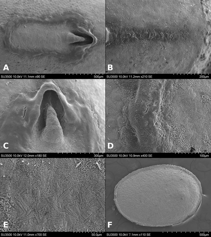
Microestructura: (n = 1) (figs. 14, 15) cápsula con superficie dorsal cubierta por paralelepípedos (fig. 14A, B) con longitudes de arista entre 6-9.5 μm (fig. 14E, F). En las superficies laterales y ventrales es lisa (fig. 14C, D). Lámina micropilar en general con textura lisa hacia el centro (fig. 15A); con tendencia a formar fibras que se vuelven una retícula hacia la periferia (fig. 15B). Tubérculo micropilar lineal, liso, con 273 μm de longitud y 108 μm de amplitud aproximadamente (fig. 15C). El borde es el límite entra las texturas de la lámina micropilar y la cápsula. Sin copa micropilar, ni línea media. Opérculo de textura como en la cápsula (fig. 15D).
Pseudosermyle sp. 4 (figs. 1, 6E, 7E, 16, 17)
Material examinado: 15 huevos disecados y 3 ootecas. México, Guanajuato, Silao de la Victoria, Villa Esmeralda, 20°57’13.212” N, 101°26’0.996” O, 1,782 m snm [voucher: PHMX 359-373, 423-425 depositados en CNIN y MZFC].
Medidas en μm: (n = 15) L= 3604.68 ± 54.49 (3488.4-3672), W= 1324.98 ± 48.65 (1239.3-1377), H = 1499.4 ± 72.91 (1377-1606.5), mpl = 633.42 ± 107.22 (321.3-734.4), mpw = 535.5 ± 96.07 (229.5-596.7), oph = 859.86 ± 21.01 (826.2-872.1), opw = 694.62 ± 29.37 (642.6-734.4), %h/l (elongación) = 41.61 ± 2.29 (38.46-46.05), %w/h (compresión) = 88.57 ± 5.66 (79.41-100).
Microestructura: (n = 1) (figs. 16, 17) cápsula de superficie dorsal cubierta por paralelepípedos (fig. 16A, B), con longitudes de arista entre 1-3 μm (fig. 16E, F). En las superficies laterales y ventral con una reducción gradual de los paralelepípedos (fig. 16C, D). Lámina micropilar en general de textura lisa hacia el tubérculo micropilar; hacia el borde es rugosa (fig. 17A). Tubérculo micropilar liso, con 321 μm de longitud y 136 μm de amplitud aproximadamente (fig. 17C).
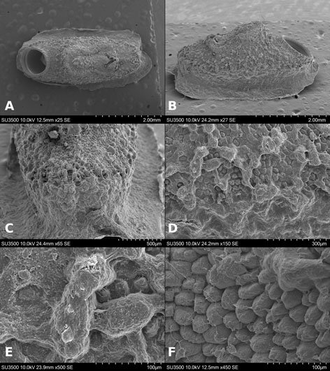
El borde es una ligera elevación que rodea la lámina micropilar y se encuentra abierto en el área polar (figs. 16C, 17A); su textura es rugosa (fig.17B), de aproximadamente 64 μm de amplitud. Sin copa micropilar, ni línea media (figs. 16C, 17A). Opérculo de textura como en la cápsula (fig. 17D).
Pseudosermyle grupo 3
Huevo: alveolar, de oviposición por caída (fig. 5A), doliforme. Medidas en mm (n = 79): L = 2.14 ± 0.14 (1.82-2.41), W = 1.44 ± 0.11 (1.14-1.64), H = 1.61 ± 0.1 (1.38-1.79), mpl = 1.03 ± 0.09 (0.85-1.26), mpw = 0.5 ± 0.07 (0.38-0.64), oph = 1.05 ± 0.09 (0.82-1.29) y opw = 0.89 ± 0.09 (0.67-1.05). Lámina micropilar en general oblonga y con una longitud cercana a la mitad de la longitud de la cápsula. Lámina micropilar interna abierta con línea media (fig. 6F-I).
Especies incluidas: Pseudosermyle carinulata (Brunner von Wattenwyl, 1907), P. striata (Burmeister, 1838), Pseudosermyle sp. 5 y se incluye a Nooxapty isabelae López-Mora et Llorente-Bousquets, 2023 como parte de este grupo debido a su similitud coriónica, aunque la microestructura es más especializada.
Pseudosermyle carinulata (Brunner von Wattenwyl, 1907) (figs. 1, 6F, 7F, 18, 19)
Material examinado: 7 huevos. México, Edo. de México, Valle de Bravo, bajo mesa, 19°5’9.96” N, 100°4’35.94” O, 2, 201 m snm [voucher: PHMX 416-422 depositados en CNIN y MZFC].
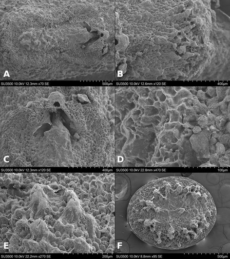
Medidas en μm: (n = 7) L = 1961.4 ± 89.35 (1822.8-2058), W = 1327.2 ± 82.15 (1176-1411.2), H = 1528.8 ± 83.15 (1381.8-1587.6), mpl = 970.2 ± 48 (911.4-1029), mpw = 399 ± 23.13 (382.2-441), oph = 919.8 ± 50.1 (823.2-970.2), opw = 806.4 ± 41.07 (735-852.6), %h/l (elongación) = 77.93 ± 1.96 (74.6-79.41), %w/h (compresión) = 86.78 ± 1.4 (84.9-88.88).
Microestructura: (n = 1) (figs. 18, 19) cápsula de superficie granulosa (fig. 18A, B), con gránulos de diámetro entre 25.7-50.3 μm (fig. 18D), toda la superficie está cubierta por proyecciones digitiformes de altura entre 1.2-2.1 μm y una separación entre ellos de 0.7-3 μm (fig. 18E, F). Lámina micropilar de superficie como en la cápsula (fig. 19A), aunque los gránulos son de textura verrugosa (fig. 19E), el espacio entre los gránulos muestra la misma textura que aquellos de la cápsula (fig. 19E). Borde de una superficie con gránulos menos marcados y con un surco circumperiférico que lo separa del centro de la lámina micropilar (fig. 19A, D), con proyecciones digitiformes muy separadas, mide 76 μm de amplitud. Tubérculo micropilar como una giba más o menos rectangular de 97 μm de longitud y 69 μm de amplitud, su textura es verrugosa (figs. 18A, 19A). Copa micropilar separada del borde, con forma de ‘u’ abierta de 145 μm de amplitud y 22 μm de grosor (fig. 19C). Línea media como una carina de 31 μm de amplitud (figs. 18C, 19B). Las últimas 2 estructuras son de textura verrugosa. Opérculo de superficie granulosa (fig. 19F); la textura de los gránulos es similar a los que tiene la cápsula.
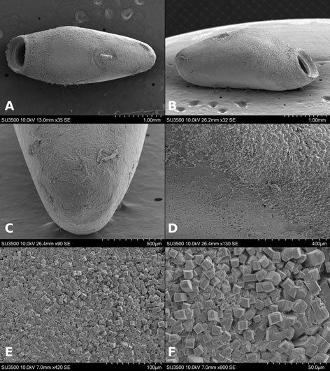
Pseudosermyle striata (Burmeister, 1838) (figs. 1, 6G, 7G, 20, 21)
Material examinado: 45 huevos. México, Puebla, Cuetzalan del Progreso, camino a Tzinacapan, 20°0’59.6088” N, 97°32’23.388” O, 657 m snm [voucher: PHMX 259-303 depositados en CNIN y MZFC]
Medidas en μm: (n = 45) L = 2212.18 ± 91.94 (2028.6-2410.8), W = 1486.98 ± 60.92 (1323-1587.6), H = 1641.82 ± 73.35 (1470-1764), mpl = 1051.21 ± 101.48 (852.6-1264.2), mpw = 529.2 ± 36.54 (441-588), oph = 1069.5 ± 56.16 (940.8-1176), opw = 939.49 ± 51.28 (793.8-1058.4), %h/l (elongación) = 74.21 ± 3.24 (67.53-81.69), %w/h (compresión) = 90.56 ± 3.1 (81.35-98.03).
Microestructura: (n = 1) (figs. 20, 21) cápsula de superficie rugosa en general (fig. 20A, B), con arrugas que varían en tamaño entre 70-170 μm de longitud y 10-45 μm de amplitud (fig. 20D); estas estructuras están cubiertas por una retícula (fig. 20E) donde en cada intersección se produce una proyección cilíndrica o cónica de 1-3 μm de alto y una separación entre ellas de 1-3 μm (fig. 20F); con gránulos alrededor de la lámina micropilar cuyo diámetro mide entre 20-28 μm (figs. 20A, 21A), con textura similar a las arrugas. Lámina micropilar de textura rugosa (fig. 21E), con las arrugas hacia el centro y coliculada hacia el borde (fig. 21A). Borde a modo de carina periférica (fig. 21A); mide 13 μm de amplitud (fig. 21D).
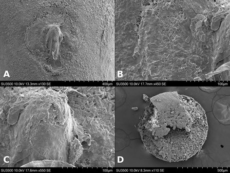
Tubérculo micropilar en forma de triángulo invertido, mide 191 μm de longitud y 128 μm de amplitud (fig. 21A). Copa micropilar separada del borde, con forma de ‘u’ abierta; comienza donde termina el borde, mide 171 μm de amplitud y 24 μm de grosor (fig. 21C). Línea media es una carina con un surco en medio a lo largo, mide 56 μm de amplitud (figs. 20C, 21B). La textura de todas las estructuras anteriores es similar a la que exhiben las arrugas de la cápsula. Opérculo de composición similar a la cápsula, las arrugas suelen ser menos prominentes hacia el centro, el borde del opérculo es una carina periférica (fig. 21F). La textura es similar a la que poseen las arrugas de la cápsula.
Pseudosermyle sp. 5 (figs. 1, 6H, 7H, 22, 23)
Material examinado: 15 huevos. México, Puebla, Cuetzalan del Progreso, camino a Tzinacapan, 20°0’59.6088” N, 97°32’23.388” O, 657 m snm [voucher: PHMX 374-388 depositados en CNIN y MZFC].
Medidas en μm: (n = 15) L = 1969.8 ±89.58 (1822.8-2087.4), W= 1277.92 ± 59.7 (1146.6-1352.4), H = 1495.48 ± 39.85 (1440.6-1587.6), mpl = 1048.6 ± 99.8 (911.4-1234.8), mpw = 392 ± 14.34 (382.2-411.6), oph = 966.28 ± 39.85 (911.4-1029), opw = 746.76 ± 45.54 (676.2-823.2), %h/l (elongación) = 76 ± 2.32 (71.83-79.36), %w/h (compresión) = 85.44 ± 3.02 (79.59-90).
Microestructura: (n = 1) (figs. 22, 23) cápsula de superficie rugosa en general (fig. 22A, B), con arrugas que varían en tamaño, mide entre 67-185 μm de longitud y 9-35 μm de amplitud (fig. 22D, E); estas estructuras están cubiertas por una textura rugulosa con orificios irregulares que varían en diámetro de 0.5-3.2 μm (fig. 22F). Lámina micropilar de superficie como en la cápsula (fig. 23A, E). Borde como un surco de 4.8 μm de amplitud (fig. 23D). Tubérculo micropilar como una giba más o menos rectangular, con 123 μm de longitud y 69 μm de amplitud (fig. 23A). Copa micropilar separada del borde, en forma de ‘u’ abierta, mide 187 μm de amplitud y 54 μm de grosor (fig. 23C). Línea media a modo de carina, mide 35 μm de amplitud (figs. 22C, 23B). La textura es similar a la que muestran las arrugas de la cápsula. Opérculo rugoso (fig. 23F), con arrugas similares a las que exhibe la cápsula y con la misma textura.
Nooxapty isabelae López-Mora et Llorente-Bousquets, 2023 (figs. 1, 6I, 7I, 24, 25)
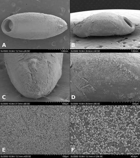
Material examinado:12 huevos. México, Oaxaca, Totontepec Villa de Morelos, curva 1 Amatepec-Chinantequilla, 17°17’5.46” N, 95°59’18.1032” O, 1,562 m snm [voucher: PHMX 389-400 depositados en CNIN y MZFC].
Medidas en μm (n = 12): L = 2234.4 ± 77.27 (2116.8-2352), W = 1538.6 ± 66.72 (1440.6-1646.4), H = 1724.8 ± 84.4 (1558.2-1793.4), mpl = 1021.65 ± 39.88 (970.2-1087.8), mpw = 590.45 ± 29.28 (558.6-646.8), oph = 1200.5 ± 66.13 (1087.8-1293.6), opw = 980 ± 60.55 (882-1058.4), %h/l (elongación) = 77.2 ± 3.18 (72.6-84.72), %w/h (compresión) = 89.28 ± 3.41 (72.6-84.72).
Microestructura: (n = 1) (figs. 24, 25) cápsula de superficie espinosa (fig. 24A, B); espinas de diámetro entre 21-38 μm y altitud entre 81-211.5 μm (fig. 24A-D). Toda la superficie está cubierta por proyecciones digitiformes de altura entre 1.5-4.5 μm y una separación entre ellos de 1.7-4.4 μm (fig. 24D-F).
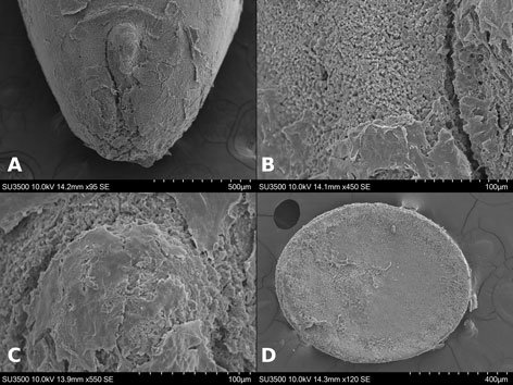
Lámina micropilar cuya ornamentación y textura es similar a la cápsula (fig. 25A). Borde a modo de carina, con una sucesión de espinas unidas (similares a las de la cápsula) (fig. 25A, D). Tubérculo micropilar en forma de ‘y’, a manera de sucesión de espinas; mide 351 μm de longitud total, 199 μm de longitud hasta la bifurcación y 145 μm de longitud en cada brazo de la ‘y’, mide 27 μm de grosor (fig. 25A). Copa micropilar separada del borde, como una ‘u’ abierta, las espinas del borde acaban en los límites de la copa micropilar; mide 153 μm de amplitud y 24 μm de grosor (fig. 25C). Línea media a modo de sucesión de espinas solitarias (figs. 24C, 25B), de amplitud igual al diámetro de las mismas (21-38 μm). La textura en todas las estructuras anteriores es similar a la que posee la cápsula (fig. 25E). Opérculo espinoso con la misma composición, textura y medidas que las espinas de la cápsula; el borde carece de espinas y exhibe un surco que encierra a todas las espinas (fig. 25F).
Pseudosermyle grupo 4
Huevo: alveolar, de oviposición por caída (fig. 5A), doliforme.
Medidas en mm: (n = 105) L = 2.68 ± 0.09 (2.37-2.92), W = 1.69 ± 0.08 (1.38-1.89), H = 1.87 ± 0.08 (1.38-1.89), mpl = 0.74 ± 0.08 (0.58-0.94), mpw = 0.4 ± 0.08 (0.25-0.54), oph = 1.43 ± 0.11 (1.16-1.75) y opw = 1.16 ± 0.09 (0.94-1.42). Lámina micropilar en general oblonga y de longitud cercana a un tercio de la longitud de la cápsula, lámina micropilar interna abierta con línea media (fig. 6J-L).
Especies incluidas: Pseudosermyle phalangiphora (Rehn, 1907), P. procera Conle, Hennemann et Fontana, 2007 y Pseudosermyle sp. 6.
Pseudosermyle phalangiphora (Rehn, 1907) (fig. 1, 6J, 7J, 26, 27)
Material examinado: 45 huevos. México, Veracruz, San Andrés Tuxtla, camino viejo EBTLT, 18°35’9.89988” N, 95°4’31.8” O, 143 m snm [voucher: PHMX 169-213 depositados en CNIN y MZFC].
Medidas en μm: (n = 45) L = 2686.4 ± 101.28 (2372.5-2920), W = 1657.1 ± 82.86 (1387-1898), H = 1826.62 ± 85.58 (1496.5-2007.5), mpl = 829.76 ± 59.46 (693.5-949), mpw = 478.55 ± 42.06 (401.5-547.5), oph = 1460.81 ± 122.66 (1168-1752), opw = 1176.11 ± 113.27 (1022-1423.5), %h/l (elongación) = 68.01 ± 2.52 (63.07-75.34), %w/h (compresión) = 90.76 ± 3.23 (84.61-101.96).
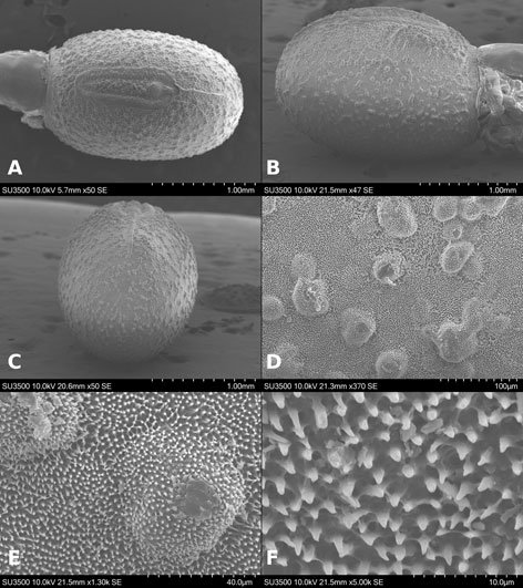
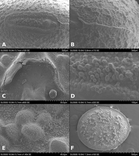
Microestructura: (n = 1) (figs. 26, 27) cápsula de superficie gibosa (fig. 26A, B), con gibas irregulares de diámetro entre 197.05-352.94 μm; suelen exhibir entre 1 y 4 poros de diámetro aproximado de 24 μm (fig. 26D), en el centro de este poro se produce una espina sombrilla (fig. 26D, E) de altura aproximada entre 44-48 μm, cuya amplitud es de 5 μm; la sombrilla de la espina formada por varios lóbulos es de diámetro aproximado de 18 μm (fig. 26E). La textura de la superficie dorsal es foveada (fig. 26D), con fóveas de 20 μm aproximadamente; éstas a su vez están punteadas con orificios de 0.5-1.8 μm de diámetro (fig. 26F); en el área polar en lugar de fóveas se forman gránulos (fig. 26C) de diámetro entre 12.5-17.18 μm.
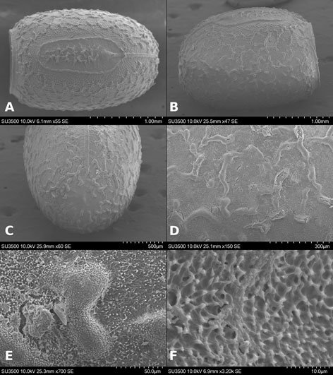
Lámina micropilar con superficie coliculada (fig. 27A) y textura rugulosa (fig. 27E). Borde como una carina de 207 μm de amplitud (fig. 27D); textura similar a la cápsula. Tubérculo micropilar similar a una media esfera de 114 μm de longitud y 153 μm de amplitud (fig. 27A); ornamentación similar a la lámina micropilar. Copa micropilar fusionada al borde con forma de ‘u’, mide 230 μm de amplitud y 129 μm de grosor (fig. 27C). Línea media a modo de carina de 179 μm de amplitud (figs. 26C, 27B). La textura de estas últimas 2 estructuras es similar a la cápsula. Opérculo muestra una giba al centro, mide 73-182 μm de longitud y entre 365-547 μm de amplitud, cuya altura es de 474-839 μm; está giba puede exhibir una muesca al centro, con esto adquiere una apariencia de pequeño cráter; en la cúspide presenta poros con espinas sombrilla del mismo tamaño y forma que los de la cápsula (fig. 27F). La textura es similar a la cápsula; en el borde se forma una carina circumperiférica (fig. 27F).
Pseudosermyle procera Conle, Hennemann et Fontana, 2007 (figs. 1, 6K, 7K, 28, 29)
Material examinado: 45 huevos. México, Veracruz, San Andrés Tuxtla, camino viejo EBTLT, 18°35’9.89988” N, 95°4’31.8” O, 143 m snm [voucher: PHMX 214-258 depositados en CNIN y MZFC].
Medidas en μm: (n = 45) L = 2715.6 ± 61.47 (2555-2810.5), W = 1747.13 ± 54.80 (1606-1825), H= 1933.68 ± 54.18 (1788.5-2044), mpl = 682.14 ± 41.77 (584-766.5), mpw = 346.34 ± 55.36 (255.5-438), oph = 1464.05 ± 83.16 (1314-1642.5), opw = 1180.16 ± 57.18 (1095-1277.5), %h/l (elongación) = 71.24 ± 2.06 (67.1-76.71), %w/h (compresión) = 90.36 ± 2.06 (83.92-94.33).
Microestructura: (n = 1) (figs. 28, 29) cápsula con superficie verrugosa (fig. 28A, B), cuyas verrugas miden de diámetro entre 40.8-289.32 μm, de textura rugulosa (fig. 28D, E), compuesta por protuberancias de diámetro de 2.42-8.53 μm (fig. 28E); entre las verrugas la superficie es foveada (fig. 28D), con fóveas de 17.68-28.06 μm de diámetro, e igual que las verrugas son de textura rugulosa (fig. 28F). Lámina micropilar de superficie escasamente coliculada (fig. 29A); textura rugulosa como la cápsula (fig. 29D). Borde a modo de carina (fig. 29A), mide 42 μm de amplitud, textura como en la cápsula (fig. 29C). Tubérculo micropilar como una media esfera de 61 μm de longitud y 80 μm de amplitud (fig. 29A); textura similar a la lámina micropilar. Copa micropilar fusionada al borde (fig. 29B), con forma de ‘u’, de 230 μm de amplitud y 159 μm de grosor, cuya textura es rugulosa. Sin línea media evidente. Opérculo con ornamentación similar a la cápsula, las verrugas forman un anillo periférico (fig. 29E); al centro la superficie es coliculada, pero mantiene la textura rugulosa (fig. 29F).
Pseudosermyle sp. 6 (figs. 1, 6L, 7L, 30, 31)
Material examinado: 15 huevos. México, Oaxaca, Santiago Choápam, curva Choápam-Latani, 17°22’39.9144” N, 95°54’58.5144” O, 701 m snm [voucher: PHMX 401-415 depositados en CNIN y MZFC].
Medidas en μm:(n = 15) L = 2584.2 ± 77.05 (2482-2701), W = 1625.46 ± 43.33 (1569.5-16.79), H = 1834.73 ± 44.63 (1752-1898), mpl = 686.2 ± 31.45 (657-766.5), mpw = 347.96 ± 23.35 (292-365), oph = 1270.2 ± 41.84 (1168-1350.5), opw = 1085.26 ± 54.25 (949-1131.5), %h/l (elongación)= 71.01 ± 1.27 (68.49-72.85), %w/h (compresión) = 88.63 ± 2.81 (84.31-93.87).
Microestructura: (n = 1) (figs. 30, 31) cápsula coliculada (fig. 30A, B) con gránulos de 31.30-51.20 μm de diámetro, superficie rugulosa con verrugas de 1.76-4.12 de diámetro (fig. 30D, F). Las espinas sombrilla por lo general en grupos de al menos 3 (fig. 30E), aunque en ocasiones se encuentran solitarias; su altura es de 47-51 μm, su amplitud entre 5.9-10 μm; la sombrilla de la espina está formada por un círculo con diámetro entre 47.64-59.24 μm (fig. 30E). Lámina micropilar con ornamentación similar a la cápsula, pero carece de espinas sombrilla (fig. 31A). Borde a modo de carina de 49 μm de amplitud (fig. 31A, D), su textura rugulosa (fig. 31D). Tubérculo micropilar como un triángulo invertido de 252 μm de longitud y 155 μm de amplitud (fig. 31A); textura similar a la lámina micropilar (fig. 31E). Copa micropilar fusionada al borde, en forma de ‘u’, mide 139 μm de longitud y 48 μm de grosor (fig. 31C), de textura rugulosa como la cápsula. Línea media como una sucesión de gránulos (fig. 31B), puede exhibir espinas sombrilla; de 322 μm de longitud y 89 μm de amplitud, de textura rugulosa. Opérculo con espinas sombrilla que forman un anillo concéntrico rodeado de textura coliculada; al centro presenta la misma textura y algunas espinas sombrilla (fig. 31F).
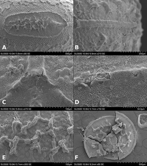
Comportamiento de oviposición. Los grupos encontrados presentan 3 comportamientos distintos de oviposición: 1) por caída, para las especies: P. striata, P. carinulata, Pseudosermyle sp. 5 y Nooxapty isabelae del grupo 3 y P. phalangiphora, P. procera y Pseudosermyle sp. 6 del grupo 4 (fig. 5A); 2) pegados en sustrato, para las especies: Pseudosermyle sp. 1, Pseudosermyle sp. 2 y Pseudosermyle sp. 3 del grupo 1 (fig. 5B); y 3) agrupados en ooteca, para las especies: P. tridens y Pseudosermyle sp. 4 del grupo 2 (fig. 5C).
Variabilidad morfológica del huevo. Los caracteres constantes entre los grupos son: tipo de oviposición, tipo de huevo, forma de la cápsula, ángulo opercular, número de capas presentes en el opérculo, porcentaje de cobertura de la longitud de la lámina micropilar (mpl) con respecto a la longitud de la cápsula (L), forma de la lámina micropilar interna y posiciones del tubérculo y copa micropilar. Por lo tanto, suponemos que son caracteres relevantes para identificar los grupos obtenidos por PCA y nos permiten definirlos. En contraste, los caracteres como ornamentación y textura de la cápsula, opérculo, lámina micropilar y línea media son caracteres variables entre especies, pero constantes entre los huevos de distintas hembras de la misma especie. Podemos suponer que estos caracteres son específicos (tablas 10-12). A continuación, se discuten a nivel de grupo los caracteres mencionados como específicos y algunas de sus posibles tendencias.
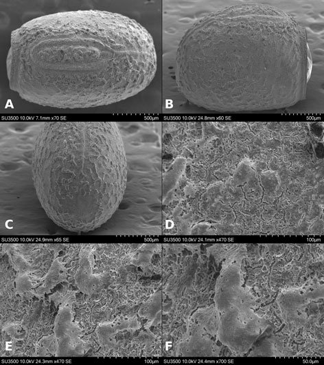
Discusión
Las especies dePseudosermyle presentan distintos tipos de morfología del huevo, lo que nos permite reconocer 4 grupos, con Nooxapty isabelae próximo al grupo 3. Se reconocen 2 tipos de huevo, alveolar (grupos 3 y 4) y adhesivos (grupos 1 y 2); con 3 comportamientos de oviposición: por caída (grupos 3 y 4), adheridos al sustrato (grupo 1) e incluidos en 1 ooteca (grupo 2); se admiten 4 grupos acorde a las medidas obtenidas por PCA, que coinciden con aquellos reconocidos cualitativamente con otras estructuras (morfología del macho y la hembra). Esta diferenciación permite proponer el reconocimiento de 4 unidades ovocíticas distintas dentro de Pseudosermyle. Se observó que dentro de cada grupo existen ciertas características comunes en la morfología del huevo (tablas 10-12); pero a su vez existen diferencias suficientes entre las especies que los conforman (tablas 10-12). Por lo tanto, se puede reconocer y diferenciar de manera inequívoca a cada especie y el grupo al que pertenece. Las ilustraciones de P. truncata y Bacteria cacica Kaup, 1871 (sinónimo deP. tridens [Hebard, 1932]) corresponden conel patrón del huevo que encontramos en el grupo 1.
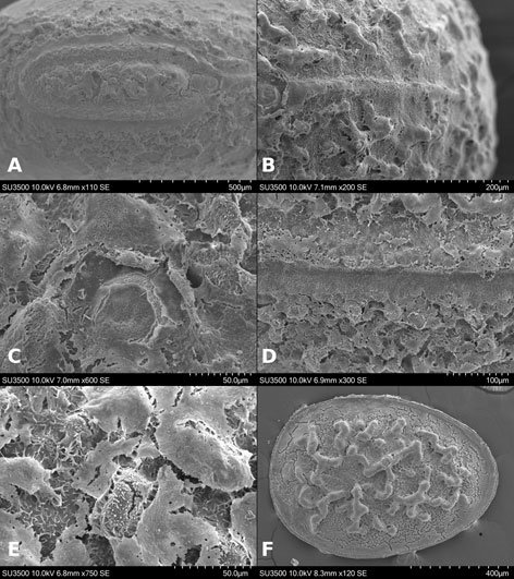
En cambio, la ilustración provista por Zompro (2001) de P. tridens sigue el patrón del grupo 2, lo que sugiere queB. cacica fue sinonimizada equivocadamente conP. tridens por Hebard (1932). Consideramos que es indispensable revisar más organismos de estas 2 especies con la finalidad de examinar esta sinonimia posiblemente errónea y reconocer a B. cacica como especie válida. Por último, P. phalangiphora corresponde con el grupo 4; no obstante, la morfología coriónica ilustrada por Conle et al. (2007) no corresponde con la encontrada en el presente trabajo. Conle et al.(2007) mencionan que esta especie es muy variable en sus genitales, por ende, una revisión detallada es necesaria para clarificar si se trata de variación intraespecífica o bien de 2 especies distintas con algunos caracteres homoplásticos.
Cabe destacar que en nuestro estudio se encontró un tipo de oviposición que previamente solo había sido registrado para la subfamilia Korinninae (hoy Necrosciinae) por Goldberg et al. (2015). Éste representa el segundo caso de formación de ooteca en Phasmatodea y a su vez una convergencia para ambos casos. Nuestros resultados representan el primer registro para América y el primero en la familia Diapheromeridae. Hay diferencia entre las ootecas de ambos taxones referente a la forma en la que los huevos están acomodados; mientras en Korinninae los huevos están acomodados de forma radial y se generan 4 cámaras, en nuestro caso, en el grupo 2de Pseudosermyle están acomodados en líneas sin formación de cámaras.
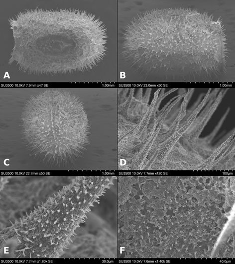
Debido a que las especies con ootecas, en este estudio, provienen de ambientes con temporada seca muy marcada como el matorral xerófilo y la selva baja subcaducifolia, deducimos que la formación de una ooteca con cápsula muy dura y ancha posiblemente evita que los huevos se desequen; tal como Salas-Araiza et al. (2013) reportan para algunos Acrididae hallados en matorral xerófilo, pues se trata de una adaptación a medios xéricos. Otro aspecto importante del fenómeno es que una condición previa a la formación de una ooteca es la presencia de huevos pegados a un sustrato, tal y como lo mencionan Robertson et al. (2018); en nuestro caso, también encontramos ese comportamiento de oviposición (grupo 1) en el mismo género donde se presentan ootecas. Para poner a prueba esta aseveración, es necesario realizar un análisis filogenético donde se incluyan más especies de Pseudosermyle y así examinar el proceso en términos de posibles tendencias evolutivas, de acuerdo con las secuencias reconocidas.
El huevo en Pseudosermyle es diferente en todas las especies respecto a su forma, texturas y la disposición de sus ornamentaciones, que son exclusivas de cada especie; además, estas características se agrupan en patrones más generales, que reconocemos como grupos. Asimismo, estos caracteres son constantes entre los huevos de distintas hembras de la misma especie. Dentro de Phasmatodea, las hembras de muchas especies son muy similares y el huevo ha sido un primer paso para reconocer si pertenecen a la misma o a distintas especies. A continuación, se listan los casos donde este carácter fue útil como primer paso en el reconocimiento de especies muy similares.
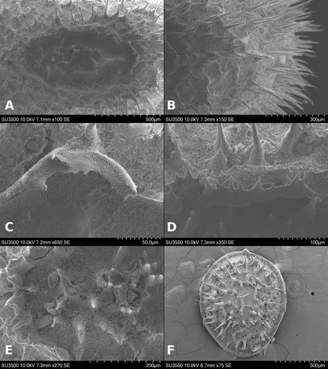
El primer caso corresponde con P. striata y Pseudosermyle sp. 5, donde son simpátridas e incluso los machos se parecen mucho. Al inicio, se pensó que pertenecían a la misma especie, hasta que se analizaron los huevos bajo el estereoscopio y el MEB. Se registró que los huevos eran diferentes en varios aspectos, como la ornamentación y la textura de la cápsula, la forma de la lámina micropilar y el opérculo. Entonces, para corroborar que se trataba de 2 especies distintas, se realizó la técnica descrita en materiales y método, con lo cual se confirmó nuestra hipótesis.
El segundo caso se dio entre P. phalangiphora y P. procera, que también son simpátridas. Se realizó el mismo procedimiento descrito en materiales y método. Las diferencias entre los huevos fueron la ornamentación de la cápsula, el opérculo y la presencia del relieve micropilar. En este caso, las diferencias entre machos eran conspicuas, así que la pregunta fue ¿cuál hembra y qué huevo correspondía a qué macho? Al igual que en el caso anterior, la respuesta se obtuvo al criar separadamente las ninfas eclosionadas de las 2 morfologías tal y como se describe en materiales y método. Después de obtener los adultos se pudo asignar a las hembras con sus respectivos machos y confirmar la continuidad morfológica con la reproducción.
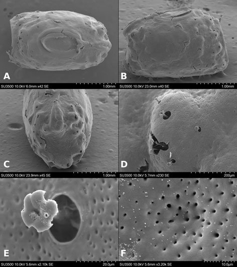
El tercer caso es entre P. tridens y Pseudosermyle sp. 4, las diferencias entre machos suelen ser igual de sutiles que las mostradas entre hembras. En ese caso, las especies no son simpátridas y se pensaba que ambas eran una única especie, pues presentaban oviposición en ooteca y morfología genital similar. Por esta causa se recurrió a la disección de hembras para obtener los huevos y realizar la comparación; entonces se encontraron las primeras diferencias, pues la lámina micropilar de P. tridens es circular y está cerca del centro de la cápsula; la lámina de Pseudosermyle sp. 4 es un triángulo invertido desplazado al área polar. Para corroborarlo se obtuvo la primera generación de Pseudosermyle sp. 4, donde las hembras y los machos presentaban la misma morfología que los parentales; también se observó que los huevos tenían la misma morfología. El cultivo de P. tridens no se logró; cabe mencionar que fue hasta la observación de los huevos que se pudo determinar a P. tridens, pues el huevo es similar a la ilustración de Zompro (2001).
Con estos casos verificamos que la afirmación de Robertson et al.(2018) sobre la especificidad del huevo a nivel de especie es cierta para este clado de Phasmatodea. Al seguir esta aseveración pudimos notar que la imagen presentada porConle et al.(2007) del huevo de P. phalangiphora de un cultivo de Belice, puede ser una especie distinta a la que reconocemos aquí como P. phalangiphora.
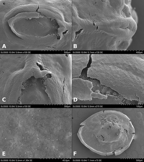
Sin embargo, es complicado conocer la identidad con certeza, pues los autores anteriores mencionan que esta especie presenta gran variabilidad en los caracteres masculinos y femeninos; en consecuencia, aquí reconocimos a los ejemplares que entraban dentro del rango de variabilidad de P. phalangiphora como esta especie, aunque una revisión más exhaustiva de los caracteres de ésta y otras poblaciones es indispensable.
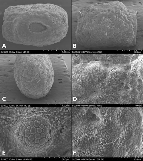
Los grupos 1 y 3 exhiben gránulos, pero la diferencia entre sus texturas es lo que los diferencia, pues el grupo 1 presenta gránulos como basamentos piramidales y el grupo 3 como semicírculos. También se observa una tendencia a aumentar o disminuir el número de niveles en el basamento piramidal y por lo tanto el tamaño del gránulo en el grupo 1; por el momento, hacen falta estudios comparativos que incluyan más especies, para después postular una posible tendencia (aumentar o disminuir el número de niveles en los basamentos piramidales) a este carácter, después de un ulterior análisis filogenético. El grupo 2 presenta especies que carecen de copa micropilar y línea media.
El grupo 3 se aproxima al género Nooxapty, por lo que se podría sugerir que al menos a nivel de medidas coriónicas son similares en forma. Este grupo exhibe gran variación en la microestructura coriónica de sus estructuras (tablas 10-12). La diferencia mayor entre Nooxapty y el grupo 3 es la presencia de espinas en el primero y de gránulos en el segundo. Se reconoce una tendencia de los gránulos a formar arrugas, pero se carece de hipótesis filogenética del género, que nos permita realizar una comparación precisa sobre tal tendencia. Además, el hecho que Nooxapty esté agrupado dentro de este grupo sugiere la necesidad de revisar estos caracteres bajo un enfoque filogenético, para aclarar si la similitud morfológica se debe a simplesiomorfías o a convergencia. Consideramos que un análisis filogenético nos permitiría contrastar y conocer los alcances de las medidas coriónicas, la ornamentación y la microestructura al momento de definir los géneros en Phasmatodea.
El grupo 4, al igual que el 3, exhibe gran variación en su microestructura coriónica (tablas 10-12). Bradler (2009) agrupa las 2 especies (P. phalangiphora y P. incongruens [Brunner von Wattenwyl, 1907]) dentro del género Pseudosermyle por presentar cercos asimétricos y con 2 ápices.Las demás, P. neptuna (Brunner von Wattenwyl, 1907), P. tridens (cercos con 3 ápices)y P. striata (con cercos simples), junto con este clado, forman un grupo monofilético a manera de peine, cuya sinapomorfía es la reducción del segundo esclerito del “poculum”. En particular, consideramos que tal variación en los cercos es muy grande y podría estar agrupando entidades distintas, por ejemplo, géneros distintos. En el presente trabajo mostramos evidencia que sustenta la formación de 4 grupos al usar la morfología coriónica y que cualitativamente observamos una correspondencia entre estos grupos y la morfología de los adultos. Sin embargo, se debe poner a prueba esta hipótesis bajo un enfoque filogenético que incluya más grupos de caracteres (v. gr. genitales internos) y especies.
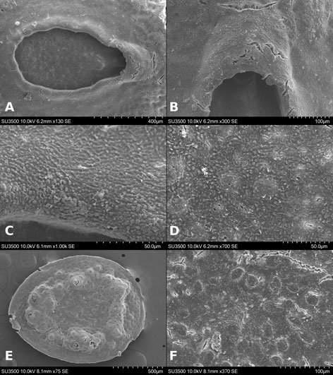
A grandes rasgos, los caracteres como textura, forma de tubérculo micropilar, borde de la lámina micropilar, línea media externa y ornamentación (tablas 10-12) son de utilidad específica entre las especies. Para hacer más robusta esta hipótesis es necesario poner a prueba estos caracteres bajo un análisis filogenético, en el cual se deben considerar más especies de cada grupo. En los análisis previos, los grupos 1, 2 y 3 solo están representados por una especie y el grupo 4 por 2 especies (Bradler, 2009); mientras que el grupo 4 se ha incluido en análisis que consideran a todo Phasmatodea (Goldberg et al. 2015; Robertson et al. 2018) y Pseudosermyle no se incluyó en los análisis de Whiting et al. (2003) y Bradler et al. (2014), pese a ser el género con mayor diversidad en América del Norte (de Luna, 2022); esto evidencia la falta de información en un género tan ampliamente distribuido.
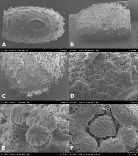
Medidas coriónicas. Cuando aplicamos PCA a las medidas de huevo (L, W, H, mpl, mpw, oph y opw) obtuvimos 4 agrupaciones, que corresponden con los patrones generales del huevo explicados anteriormente. Al revisar la contribución de las variables a cada componente (fig. 4), nos percatamos de que la longitud de la cápsula (L), la altitud (oph) y amplitud (opw) del opérculo, así como la longitud micropilar (mpl) son las medidas coriónicas que mejor explican la variación de la forma del huevo. Podemos observar que L es una variable independiente de las restantes y la que más contribuye al componente 1 (fig. 4); mientras que oph y opw están más correlacionadas positivamente con la amplitud (W) y altitud (H) de la cápsula, las variables que más contribuyen al componente 2 (fig. 4). En cambio, mpl es la variable que más contribuye al componente 3 (fig. 4) y su correlación es inversamente proporcional a oph y opw; podemos destacar que cada estructura del huevo (cápsula, lámina micropilar y opérculo) está aportando una de las medidas que lo caracterizan. En consecuencia, recomendamos que al momento de realizar descripciones del huevo se incluyan todas las medidas mencionadas.
Las medidas del huevo nos permiten distinguir 4 grupos, que además son congruentes con otros caracteres. Esto podría indicar que el género Pseudosermyle pueda estar conformado por géneros distintos, como lo sugiere Conle et al. (2007), quienes llegan a esta conclusión debido a la variabilidad de formas en los genitales de los machos. Ellos admiten que el conocimiento del género es fragmentado, en consecuencia, no realizan una redescripción del mismo. Así también, ninguna de las especies que ellos describen sigue la descripción original de Pseudosermyle pues no cumplen con las características que menciona Caudell (1903); sin embargo, coinciden con la redescripción que realizó Zompro (2001). En contraste, resaltamos que las medidas por sí solas no son suficientes en la caracterización del huevo pues N. isabelae, por sus medidas, se aproxima al grupo 3, pero al revisar la microestructura notamos que la ornamentación es distinta entre esta especie y las restantes dentro del grupo, pues exhibe espinas, mientras que las demás presentan arrugas y gránulos. En conclusión, notamos que la microestructura, como sugieren Mazzini y Scali (1983), es bastante útil al reconocer especies cercanas dentro del mismo género.
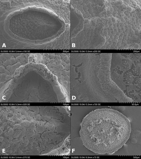
Por último, es importante destacar que Pseudosermyle exhibe gran variabilidad en los caracteres morfológicos del huevo, por lo cual consideramos que para aclarar si estos caracteres nos permiten inferir distintos géneros o representan variabilidad dentro del mismo, es indispensable revisar más caracteres, v. gr., genitales externos e internos para ambos sexos y observar una correspondencia entre los mismos. Así mismo, es necesario efectuar un análisis filogenético que nos permita postular hipótesis evolutivas sobre el género y sus caracteres o rasgos. Las especies restantes de Pseudosermyle no fueron incluidas en este trabajo debido a la carencia de tiempo y recursos para recolectar un área tan vasta como México, América Central y el sur de Estados Unidos. Por lo tanto, en el futuro será oportuno un trabajo más exhaustivo que incluya lo antes mencionado y amplíe el número de especies analizadas. Aún queda mucho trabajo por realizar con Pseudosermyle, pues al igual que muchos géneros de Phasmatodea americanos, se desconoce su bionomía.
Agradecimientos
Al posgrado en Ciencias Biológicas, UNAM, por el financiamiento a la beca de Secihti (cvu: 599426 y cvu: 1039296). A Susana Guzmán Gómez por la asistencia técnica en las micrografías en el Laboratorio de Microscopia y Fotografía de la Biodiversidad II, IB UNAM. A Arturo Arellano Covarrubias por la asesoría en la realización del mapa. A Isabel Vargas Fernández y María Berenit Mendoza Garfias por su asistencia técnica al montar las muestras y tomar las fotomicrografías con microscopio electrónico de barrido. Isabel Vargas ayudó críticamente en la elaboración de las figuras. JLB agradece al proyecto PAPIIT-UNAM IN 202415. ULM agradece a la Orthopterists Society por el Theodore J. Cohn Research Fund. Por último, agradecemos a 2 revisores anónimos en la revisión previa del presente manuscrito.
Referencias
Adler, D., Murdoch, D. Nenadic, O., Urbanek, S., Chen, M., Gebhardt, A. et al. (2018). rgl: 3D Visualization Using OpenGL. R package version 0.99.16. Recuperado el 10 junio 2019 de: https://cran.r-project.org/web/packages/shinyRGL/index.html
Allred, M. L., Stark, B. P. y Lentz; D, L. (1986). Egg capsule morphology of Anisomorpha buprestoides (Phasmatodea: Pseudophasmatidae). Entomological News, 97, 169–174.
Bradler, S. (2009). Die Phylogenie der Stab- und Gesepnstruchrecken (Insecta: Phasmatodea). Species, Phylogeny and Evolution, 2, 3–139. https://doi.org/10.17875/gup2009-710
Bradler, S. y Buckley, T. R. (2018). Biodiversity of Phasmatodea. En R. G. Foottit y P. H. Adler (Eds.), Insect biodiversity: science and society, Volumen II (pp. 281–313). Ottawa: Jonh Wiley & Sons Ltd. https://doi.org/10.1002/9781118945582.ch11
Bradler, S., Robertson, J. A. y Whiting, M. F. (2014). A molecular phylogeny of Phasmatodea with emphasis on Necrosciinae, the most species-rich subfamily of stick insects. Systematic Entomology, 39, 205–222. https://doi.org/10.1111/syen.12055
Brock, P. D., Büscher, T. y Baker; E, (2023). Phasmida Species File Online. Versión 5.0/5.0 Recuperado el 20 abril 2019 de: https://phasmida.speciesfile.org/
Camousseigth, A. y Bustamante, I. (1991). Descripción de los huevos de los fásmidos (Phasmatodea: Pseudophasma-
tidae) de Chile. Revista Chilena de Entomología, 19, 39–43.
Caudell, A. N. (1903). The Phasmidae or walkingsticks, of the United States. Proceedings of the United States National Museum, 26, 863–885. https://doi.org/10.5479/si.00963801.26-1335.863
Caudell, A. N. (1914). The egg of Pseudosermyle truncata Caudell. Proceedings of the Entomological Society of Washington, 16, 96.
Clark, J. T. (1976a). The capitulum of phasmid eggs (Insecta: Phasmida). Zoological Journal of the Linnean Society, 59, 365–614. https://doi.org/10.1111/j.1096-3642.1976.tb01019.x
Clark, J. T. (1976b). The eggs of stick insects (Phasmida): a review with descriptions of the eggs of eleven species. Systematic Entomology, 1, 95–105. https://doi.org/10.1111/j.1365-3113.1976.tb00342.x
Clark, J. T. (1979). A key to the eggs of stick and leaf insects (Phasmida). Systematic Entomology, 4, 325–331. https://doi.org/10.1111/j.1365-3113.1979.tb00617.x
Conle, O. V., Hennemann, F, H. y Fontana, P. (2007). Studies on Neotropical Phasmatodea V: notes on certain species of Pseudosermyle Caudell, 1903, with the descriptions of three new species from Mexico (Phasmatodea: Diapheromeridae: Diapheromerinae: Diapheromerini). Zootaxa, 1496,31–51. https://doi.org/10.11646/zootaxa.1496.1.2
de Luna, M. (2022). Checklist of stick insects (Insecta: Phasmatodea) of North America, with three new records for Nuevo León, México. Phasmid Studies, 21, 90–105.
GNU Image Manipulation Program (GIMP 2.8.22). Recuperado el 10 junio 2019 de: https://www.gimp.org/
Goldberg, J., Bresseel, J., Constant, J., Kneubühler, B., Leubner, F., Michalik, P. et al. (2015) Extreme convergence in egg-laying strategy across insect orders. Scientific Reports, 5, 7825. https://doi.org/10.1038/srep07825
Harris, R. A. (1979). A glossary of surface sculpturing. Occasional Papers in Entomology, 28,1–31.
Hebard, M. (1932). New species and records of Mexican Orthoptera. Transactions of the American Entomological Society, 58,201–219.
Horikoshi, M. y Tang, Y. (2016). ggfortify: data visualization tools for statistical analysis results. Recuperado el 10 de junio de 2019 de: https://doi.org/10.32614/cran.package.ggfortify
Jintsu, Y., Uchifune, T. y Machida, R. (2010). Structural features of egg of the basal Phasmatodean Timema monikensis Vickery et Sandoval, 1988 (Insecta: Phasmatodea: Timematidae). Arthropod Systematics & Phylogeny, 68, 71–78. https://doi.org/10.3897/asp.68.e31716
Kaup, J. (1871). Ueber die Eier der Phasmiden. Berliner Entomologische Zeitschrift, 15, 17–24. https://doi.org/10.
1002/mmnd.18710150106
López-Mora, U. y Llorente-Bousquets, J. (2018). Lista de especies y clave ilustrada de los géneros de Phasmato-
dea (Insecta) de México. Revista Mexicana de biodiversidad, 89, 46–78. https://doi.org/10.22201/ib.2007
8706e.2018.1.2175
López-Mora, U. y Llorente-Bousquets, J. (2023). Nooxapty gen. nov. con dos especies nuevas (Phasmatodea: Diapheromeridae) de Oaxaca, México. Dugesiana, 30, 11–33. https://doi.org/10.32870/dugesiana.v30i1.7272
Mazzinni, M., Carcupino, M. y Fausto, A. M. (1993). Egg chorion architecture in stick insects (Phasmatodea). International Journal of Insect Morphology and Embriology,22, 391–415. https://doi.org/10.1016/0020-7322(93)90021-r
Mazzini, M., Nascetti, G. y Bullini, L. (1982). The egg of the stick-insect Bacillus atticus caprai Nascetti et Bullini: a scanning electron microscope study (Cheleutoptera Bacillidae). Italian Journal of Zoology, 16, 93–103. https://doi.org/10.1080/01688170.1984.10510070
Mazzini, M., Nascetti, G. y Bullini, L. (1984). A scanning electron microscope study on the egg of a hybrid stick-insect (Cheleutoptera, Bacillidae). International Journal of Invertebrate Reproduction and Development, 7, 43–49. https://doi.org/10.1080/01688170.1984.10510070
Mazzini, M. y Scali, V. (1977). Fine structure of the insect micropyle. Scannin electron microscope investigations of the egg of the stick insect Bacillus rossius (Rossi) (Insecta Cheleutoptera). Monitore Zoologico Italiano-Italian Journal of Zoology, 11, 71–82. https://doi.org/10.1016/0020-7322(77)90020-4
Mazzini, M. y Scali, V. (1980). Eggs of the stick insects, Lonchodes pterodactylus Gray and Carausius morosus Br. (Phasmatodea: Heteronemiidae). International Journal of Insect Morphology & Embriology,9, 369–382. https://doi.org/10.1016/00207322(80)90010-0
Mazzini, M. y Scali, V. (1983). A scanning electron microscope study of the eggs of three stick insect species of Ramulus (Phasmatodea Heteronemiidae) from Somalia. Italian Journal of Zoology, 17, 89–103.
Nieves-Uribe. S., Llorente-Bousquets, J. y Flores-Gallardo, A. (2021). Toward standards in practices and techniques on ootaxonomy in the Pieridae (Lepidoptera: Papilionoidea). Zootaxa,4985, 301–344. https://doi.org/10.11646/zootaxa.4985.3.1
Ooms, J. (2018). magick: advanced graphics and image-processing in R. R package version 2.0. Recuperado el 10 junio 2019 de: https://CRAN.R-project.org/package=magick https://doi.org/10.32614/cran.package.magickgui
QGIS Dveelopment Team, (2019). QGIS Geographic Information System. Open Source Geospatial Foundation Project. Recuperado el 10 junio 2019 de: https://qgis.org.
R Core Team. (2013). R: a language and environment for statistical computing. R foundation for Statistical Computing, Vienna, Austria. Recuperado el 10 junio 2019 de: http://www.R- project.org/
Robertson, J. A., Bradler, S. y Whiting, M. F. (2018). Evolution of oviposition techniqus in stick and leaf insects (Phasmatodea). Frontiers in Ecology and Evolution, 6, 2016. https://doi.org/10.3389/fevo.2018.00216
RStudio Team (2015). RStudio: Integrated Development for R. RStudio, Inc., Boston, MA. Recuperado el 10 de junio de 2019 de: http://www.rstudio.com/. https://doi.org/10.4135/9781526472557
Salas-Araiza, M. D., Mackay, W. P., Valdez-Carrasco, J., Salazar-Solís; E, y Martínez-Jaime, O. A. (2013). Characterization and comparison of the eggs of seven species of Mexican grasshoppers. Southwestern Entomologist, 38,267–274. https://doi.org/10.3958/059.038.0210
Scali, V. y Mazzini, M. (1977). Fine morphology and amino acid analysis of the egg capsule of the stick insect, Clonopsis gallica (Charp.) (Cheleutoptera: Bacillinae). International Journal of Insect Morphology and Embryology, 6,
255–264. https://doi.org/10.1016/0020-7322(77)90020-4
Scali, V. y Mazzini, M. (1981). The eggs of stick insects, Sipyloidea sipylus (Westwood) and Orxines macklotti De Haan (Phasmatodea, Heteronemiidae). International Journal of Invertebrate Reproduction, 4, 25–38. https://doi.org/10.1080/01651269.1981.10553416
Scali, V. y Mazzini, M. (1982). Interpopulation differences in egg sculpturing of the stick insect, Clonopsis gallica (Charp.) (Phasmatodea: Bacillidae). International Journal of Insect Morphology and Embriology, 11, 189–195.
https://doi.org/10.1016/s0020-7322(82)80004-4
Scali, V. y Mazzini, M. (1983). Egg capsule morphology of the stick insect Burria longixipha Brunner (Phasmatodea Heteronemiidae) from Somaliland. Italian Journal of Zoology, 17, 303–312.
Seiler, C., Bradler, S. y Koch, R. (2006). Fásmidos: insectos palo e insectos hoja. España: Hispano Europea.
Sellick, J. T. C. (1994). A redefinition of the orientation terminology of phasmid eggs. Phasmid Studies, 3, 1–2.
Sellick, J. T. C. (1997a). The range of egg capsule morphology within the Phasmatodea and its relevance to the taxonomy of the order. Italian Journal of Zoology,64, 97–104. https://doi.org/10.1080/11250009709356178
Sellick, J. T. C. (1997b). Descriptive terminology of the phasmid egg capsule, with an extended key to the phasmid genera based on egg structure. Systematic Entomology,22, 97–122. https://doi.org/10.1046/j.1365-3113.1997.d01-30.x
Sellick, J. T. C. (1997c). The “umbrella spines” and other surface projections of some phasmid eggs and some comments on phasmid taxonomy. Phasmid Studies, 6, 15–20. https://doi.org/10.1111/j.1096-3642.1988.tb01364.x
Sellick, J. T. C. (1998). The micropylar plate of the eggs of Phasmida, with a survey of the range of plate form within the order. Systematic Entomology, 23, 203–228. https://doi.org/10.1046/j.1365-3113.1998.00056.x
Severin, H. P. (1910). A study on the structure of the egg of the walking-stick Diapheromera femorata Say. Annals of The Entomological Society of America, 3, 83–92. https://doi.org/10.1093/aesa/3.2.83
Stark, B. P. y Lentz; D, L. (1986). Morphology of the egg capsule in Megaphasma dentricus (Phasmatodea: Heteronemiidae). Journal of the Kansas Entomological Society, 52, 398–401.
Whiting, M. F., Bradler, S. y Maxwell, T. (2003). Loss and recovery of wings in stick insects. Letter to Nature, 421, 264–267. https://doi.org/10.1038/nature01313
Wickham, H. (2016). ggplot2: elegant graphics for data analysis. Nueva York: Springer-Verlag.
Weiner, J. (2017). pca3d: Three dimensional PCA plots. R package version 0.10. Recuperado el 10 junio 2019 de: https://CRAN.R-project.org/package=pca3d
Zompro, O. (2001). A generic revision of the insect order Phasmatodea: the new world genera of the stick insect subfamily Diapheromeridae: Diapheromerinae = Heteronemiidae: Heteronemiinae sensu Gradley et Galil, 1977. Revue Suisse de Zoologie, 108, 189–255. https://doi.org/10.5962/bhl.part.79626
Ecología


Genetic diversity and phenotypic variation in a parasitoid wasp involved in the yucca – yucca moth interaction
C. Rocío Álamo-Herrera a, María Clara Arteaga a, *, Rafael Bello-Bedoy b
a Centro de Investigación Científica y de Educación Superior de Ensenada, Departamento de Biología de la Conservación, Carretera Tijuana-Ensenada # 3918, Zona Playitas, 22860 Ensenada, Baja California, Mexico
b Universidad Autónoma de Baja California, Facultad de Ciencias, Carretera Transpeninsular # 3917, Colonia Playitas, 22860 Ensenada, Baja California, Mexico
*Corresponding author: arteaga@cicese.mx (M.C. Arteaga)
Received: 28 February 2024; accepted: 01 July 2024
Abstract
Tri-trophic interactions between plants, herbivores, and parasitoids are a valuable model for studying how they influence the distribution of genetic diversity and phenotypic variability of the species involved. This study examines the taxonomic, morphological, and genetic diversity of parasitoid wasps involved in the Yucca–Tegeticula interaction on the Baja California Peninsula. We surveyed 35 locations across the peninsula and collected 119 parasitoid wasps. Of these, 114 were adults, while the remaining 5 were in the pupal stage. Our study identified 2 genera of wasps: Bassus sp. (Ichneumonidae; n = 8) and Digonogastra sp. (Brachonidae; n = 111). Moreover, we found moderate levels of genetic diversity within the Digonogastra population across the peninsula. Additionally, this population constitutes a single panmictic group with indications of historical demographic expansion. Phenotypically, we identified sexual dimorphism and variation associated with its different hosts and environmental heterogeneity Digonogastra’s geographical range.
Keywords: Baja California Peninsula; Genetic structure; Host-association; Morphometrics; Tri-trophic interactions
© 2024 Universidad Nacional Autónoma de México, Instituto de Biología. Este es un artículo Open Access bajo la licencia CC BY-NC-ND
(http://creativecommons.org/licenses/by-nc-nd/4.0/).
Diversidad genética y variación fenotípica en una avispa parasitoide involucrada en la interacción entre yucas y sus polillas polinizadoras
Resumen
Las interacciones tritróficas entre plantas, herbívoros y parasitoides son un modelo valioso para estudiar cómo influyen en la distribución de la diversidad genética y la variabilidad fenotípica de las especies involucradas. Este estudio examinó la diversidad taxonómica, morfológica y genética de avispas parasitoides en la interacción Yucca-Tegeticula en la Península de Baja California. El estudio se realizó en 35 localidades recolectando 119 avispas parasitoides; 114 adultos y 5 pupas. Se identificaron 2 géneros de avispas: Bassus sp. (Ichneumonidae; n = 8) y Digonogastra sp. (Brachonidae; n = 111). Se encontraron niveles moderados de diversidad genética dentro de la población de Digonogastra en toda la península, constituyendo un único grupo panmítico con indicios de expansión demográfica histórica. Fenotípicamente, identificamos dimorfismo sexual y variación asociada con sus diferentes hospederos y la heterogeneidad ambiental a lo largo de la distribución geográfica de Digonogastra.
Palabras clave: Península de Baja California; Estructura genética; Asociación al hospedero; Morfometría; Interacción tri-trófica
Introduction
Tritrophic interactions between plants, herbivores, and parasitoids have become pivotal to understanding species diversity (Abdala-Roberts et al., 2019; Godfray, 1994; Singer & Stireman, 2005). Parasitoids maintain an antagonistic relationship with insect herbivores by depositing their eggs inside or on them, ultimately leading to the death of their host (Godfray, 1994; Quicke, 2015; Resh & Cardé, 2009). These parasitoids serve as an indirect defense for plants, controlling herbivore population levels (Abdala-Roberts et al., 2019; Cuautle & Rico-Gray, 2003; Heil, 2008). Plants attract parasitoids by emitting chemical signals that indicate the presence of herbivores, which enables parasitoids to locate their prey, thus establishing mutually beneficial interactions (Heil, 2008; Kappers et al., 2011; Takabayashi & Dicke, 1996).
Multiple studies have explored how interactions among organisms affect the genetic and phenotypic variation within species (e.g., Agrawal, 2001; Carmona et al., 2015). For instance, biotic interactions may differ geographically, resulting in local selection processes and differentiation of parasitoid populations (Althoff & Thompson, 2001; Kankare et al., 2005; Stireman et al., 2005). Environmental factors or geographical distances can also determine the distribution of these variations (Althoff, 2008; Lozier et al., 2009; Stireman et al., 2005). For example, the genetic population structure of the wasp Cotesia congregata Say, 1836 (Hymenoptera: Braconidae) is related to the different plant-hosts with which it interacts (Karns, 2009). Conversely, genetic diversity in the parasitoid wasp Eusandalum sp. Ratzeburg, 1852 (Hymenoptera: Braconidae) is primarily associated with its broad geographical distribution rather than the species it interacts with (Althoff, 2008).
The interaction between Yucca Linnaeus plants, moths of the family Prodoxidae and associated parasitoids have been recorded (Althoff, 2008; Pellmyr, 2003). In this tritrophic interaction, the female moth visits Yucca flowers and lays her eggs in the ovary. Subsequently, she pollinates the stigma by depositing pollen, ensuring the formation of fruits that the moth larvae will feed on (Engelmann, 1872). During fruit production, female parasitoid wasps use their ovipositors to lay eggs on moth larvae inside fruits, paralyzing the larvae (Force & Thompson, 1984). The wasp larva feeds on the host, completes its development, and emerges from the fruit as an adult (Althoff, 2008; Crabb & Pellmyr, 2006). The interaction between Yuccas and moths have driven differentiation and diversification processes in the involved species (Althoff et al., 2012; Althoff & Segraves, 2022; Pellmyr & Leebens-Mack, 1999). However, little is known about the third trophic level of this relationship, which consists of parasitoid wasps that interact with the moth (their food source) and the plant (their shelter until hatching).
In the Baja California Peninsula, 3 Yucca species and 2 Tegeticula Zeller, 1873 species are distributed allopatrically. Yucca schidigera Roezl ex Ortgies (Asparagales: Asparagaceae) occurs in the northern part of the peninsula and is pollinated by Tegeticula mojavella Pellmyr, 1999 (Lepidoptera: Prodoxidae). Yucca valida Brandegee (Asparagales: Asparagaceae) is distributed in the central region, whereas Yucca capensis L.W. Lenz, 1998 (Asparagales: Asparagaceae) occurs in the southern part of the peninsula. Both Y. valida and Y. capensis are pollinated by Tegeticula baja Pellmyr, Balcázar-Lara, Segraves, Althoff & Littlefield, 2008 (Lepidoptera: Prodoxidae; Lenz, 1998; Turner et al., 1995). Furthermore, a region of hybrid populations of Y. valida and Y. capensis has been identified, both pollinated by T. baja (Arteaga et al., 2020). However, there are no previous records of parasitoid wasps associated with T. baja or T. mojavella populations in the Baja California Peninsula. This study aims to identify the genera of parasitic wasps associated with Tegeticula species in the peninsula. We also investigate whether the use of different hosts, such as T. mojavella and T. baja, and the environmental distribution of the wasps lead to phenotypic and genetic differentiation in the wasp populations.
Materials and methods
We visited 35 locations in the Baja California Peninsula, following the distribution of the Yucca species and their pollinators T. mojavella and T. baja (Fig. 1A, Table S1). Specifically, we surveyed 12 locations in the northern section of the peninsula, where Yucca schidigera occurs, within forest habitats of Sierra Juárez (N = 6), Sierra San Pedro Mártir (N = 4), and Chaparral (N = 2). We visited 11 locations within the central desert of the peninsula where Yucca valida are distributed. Finally, we collected samples from 12 locations in the south section of the peninsula. Eight locations were in the coastal plains of the Magdalena Plains region, where populations of Y. valida x Y. capensis are found. The remaining 4 locations were in the deciduous lowland forest of the Cape Region, where Y. capensis populations are present.
Each location was visited once between 2013 to 2015, during the fruiting season of the Yucca species. We selected approximately 10 trees per location, gathering 3 to 5 fruits from each tree. The mature fruits were collected directly from Yucca trees and placed individually within 500 ml plastic cups with mesh netting lids. Fruits were transported to the laboratory and stored in rooms at environmental conditions (approximately 25°C and 60% relative humidity). For 2 weeks, we checked each plastic cup daily for adult wasps. All adult wasps that emerged from the fruits were collected and placed in 20 ml glass vials. Following another 2 weeks, we dissected the fruits to obtain wasps pupae. All wasps were preserved in glass vials with 96% ethanol and labeled with locality and host plant species. Adult individuals were observed with a Nikon SMZ745-T stereomicroscope equipped with Lumenera’s INFINITY digital camera, and identified to genus taxonomic level using the dichotomous key provided by Sánchez et al. (1998). Two genera of parasitoid wasps from the Braconidae family were identified (Fig. 2): Bassus Fabricius, 1804 and Digonogastra Viereck, 1912.
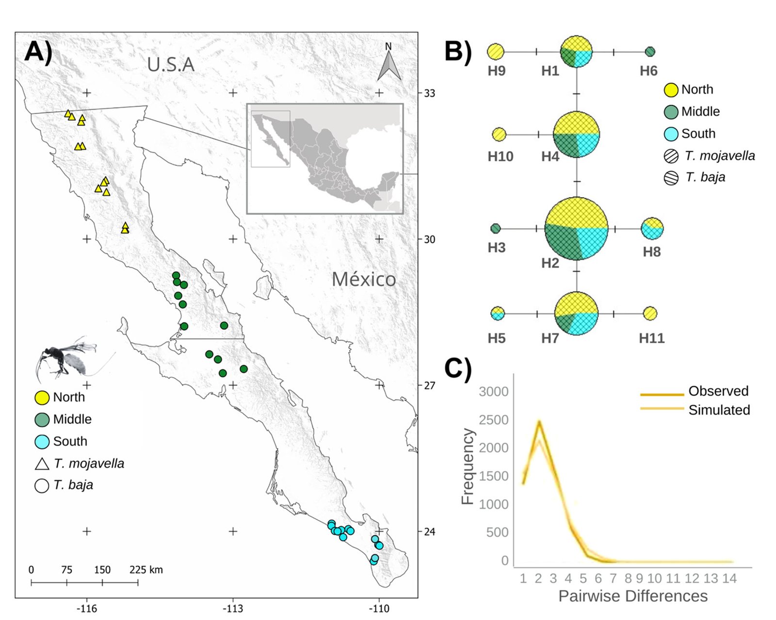
Figure 1. A, Localities sampled of Digonogastra sp. in the Baja California Peninsula. The geographical distribution is marked using colors and the host moth species is indicated whit shapes; B, haplotype network. The geographical distribution is marked using colors and the host moth species with lines; C, graph depicting the observed and simulated distribution of paired sequence differences.

Figure 2. The genera of parasitoid wasps sampled from yucca fruits in the Baja California Peninsula. On the upper side is the genus Digonogastra; on the bottom is Bassus.
DNA extraction and molecular marker amplification. We extracted DNA from 119 wasps using the commercial Qiagen DNeasy Blood & Tissue Kit. The sample consisted of 114 adult individuals and 5 in the pupal stage. A fragment of the Cytochrome Oxidase subunit I (COI) marker was amplified via PCR using the universal primers for invertebrates described by Folmer et al. (1994); LCO1490 (5’-GGTCAACAAATCATAAAGATATTGG-3’) and HCO2198 (5’-TAAACTTCAGGGTG ACCAAAAAATCA-3’). The PCR mixture included 5 µl of Buffer (1x), 1.5 µl of MgCL (2.5mM), 0.3 µl of dNTPs (0.16mM), 0.6 µl of each primer at 10 µM, 0.2 µl of Taq polymerase (1 unit), 1 µl of DNA, and 5.8 µl of molecular-grade water, resulting in a 15 µl reaction volume.
The thermal cycler was set up with the following conditions: an initial denaturation at 94 ºC for 5 min, followed by 35 cycles of denaturation at 94 ºC for 1 min, annealing at 50 ºC for 1 min, and extension at 68 ºC for 1 min. A final elongation step was performed at 72 ºC for 5 min. Amplification quality was confirmed using 1% agarose gel electrophoresis. The PCR products were sequenced by SeqXcel (www.seqxcel.com) for further analysis.
Genetic diversity and population genetic structure. The sequences were visualized, aligned, and edited using the BioEdit software (Hall, 1999). Sequences from individuals identified morphologically were submitted to BLAST to confirm the parasitoid genus (Blast.ncbi.nlm.nih.gov). The sample size of Digonogastra sp. (N = 111) allowed for diversity and population structure analysis. The genetic diversity of Digonogastra species was assessed using DNAsp software (Rozas et al., 2003). This involved calculating the number of haplotypes, haplotype diversity, and nucleotide diversity (Nei & Li, 1979; Nei, 1987). To investigate the genealogical relationships among the identified haplotypes, we constructed a haplotype network using the Median-Joining method in NETWORK 5.0 software (Bandelt et al., 1999). We constructed a phylogenetic tree using the haplotypes obtained for Digonogastra sp. to determine whether the detected diversity in the Baja California Peninsula is unique to this region or present elsewhere. We included sequences available in the NCBI from Canada. The genera Alabagrus (Sharkey & Chapman, Unpublished; GenBank: MF361682.1) and Cotesia (Hebert et al., 2016) were employed as outgroups. The tree was constructed using the Maximum Likelihood method, with 1000 bootstrap replicates and the HKY+I substitution model, which showed the best fit to the data (highest AIC value), as determined by the jModelTest program (Darriba et al., 2012).
To assess genetic differentiation of Digonogastra spp. across its geographical distribution in the peninsula, we conducted 3 Molecular Variance Analyses (AMOVA). First, we examined how geographical distances affected the distribution of genetic diversity. We divided the data into 3 categories based on their location in the peninsula: north, center, and south (Fig. 1A). Then, we assessed whether genetic differentiation was due to environmental factors, grouping the data based on their ecoregion of origin. We based our categorization on the ecoregions proposed by Gonzales-Abraham et al. (2010). Lastly, our third analysis examined whether genetic differentiation was related to the host, grouping the data based on the host moths, T. mojavella and T. baja. The ARLEQUIN software (Excoffier et al., 2005) was employed for these analyses.
We evaluated historical demographic changes in the wasp population using the pairwise sequence differences distribution analysis (mismatch analysis) performed in the ARLEQUIN software. The shape of the mismatch distribution is used to infer whether a population expansion has occurred (Rogers & Harpending, 1992). A unimodal distribution indicates population expansion, while a multimodal distribution suggests a stable population size. Additionally, the sum of squared deviations (SSD) is employed to validate the expansion model (Navascués et al., 2006). A significant SSD (p < 0.05) rejects the population expansion model.
Phenotypic variation. Phenotypic variation of the parasitoid wasps was evaluated by measuring 106 adult
individuals of the Digonogastra genus (excluding individuals in the pupal stage). No morphometric analyses were conducted for Bassus specimens due to their small sample size (N = 8). Measurements of the 106 adults were conducted with Infinity Analyze software (Lumenera, Canadá), calibrated in millimeters and verified with a conventional ruler. We measured 18 external morphological characters of the adult individuals (Table 1). Measurements were taken on the left side of the individuals and included the length from the head to the end of the last metasoma segment, the scape width, antenna length, mesosoma (thorax) and metasoma (abdomen) width and length, femur width, total leg length, anterior wing length, and the length of 5 wing vein components: C+SC+R, 1RS, (RS+M)a, 2RS, and r-rs. For females, we also measured the length and width of the ovipositor and the length of the ovipositor apex (Table 1). We calculated the mean, standard deviation, and coefficient of variation of each measured character. A correlation matrix was created using the Pearson Correlation Coefficient (r) between pairs of characters, determining the significance values (p) for each correlation. All morphometric measurements were analyzed with JMP 5.01 software (SAS Cary, New Jersey, USA).
We assessed 3 potential sources of variation for the phenotypic differentiation among parasitoid wasps in the Baja California Peninsula: sexual dimorphism, the ecoregions in which they are distributed, and the host species of Tegeticula moths. We conducted a Multivariate Analysis of Variance (MANOVA) for each factor using all measured characters. We also performed an Analysis of Variance (ANOVA) to determine which trait contributes significantly to phenotypic differences. Each wasp was assigned to an ecoregion based on its geographical origin (Gonzales-Abraham et al., 2010). The wasps were found in 6 ecoregions: Sierra Juárez, Sierra San Pedro Mártir, Chaparral, Central Desert, Magdalena Plains, and Cape Lowland Forest.
Results
We collected a total of 119 parasitoid wasps from 35 locations across the Baja California Peninsula (Fig. 1A, Table S1). Two genera of parasitoid wasps belonging to the Braconidae family were collected: Bassus and Digonogastra. Eight female individuals of Bassus sp. (6.7%) emerged from fruits in 2 different locations. Seven Bassus specimens were collected in Y. valida fruits, while 1 emerged from Y. capensis. All these fruits contained T. baja larvae. In contrast, we collected 111 Digonogastra individuals (93.3%), with 68 males and 38 females from 33 different sites across 32.58° to 23.38° N latitude. Out of these, 57 individuals of Digonogastra sp. emerged from Y. schidigera fruits where T. mojavella was also found. The remaining 54 individuals were found in Y. valida, Y. valida x Y. capensis, and Y. capensis fruits, where T. baja larvae were also present.
Table 1
Mean (M), standard deviation (SD), and coefficient of variation in percentage (CV) of the evaluated morphological traits in female and male individuals of Digonogastra sp. in the Baja California Peninsula. The results of the analysis of variance (ANOVA) performed for sexual dimorphism (S), ecoregions (E), and host (H) are presented with significance levels denoted as follows: p > 0.05 (ns), p < 0.05 (*), and p < 0.0001 (***).
| Trait | Female | Male | ANOVA | ||||||
| M | SD | CV | M | SD | CV | S | E | H | |
| Body length: | 9.03 | 1.29 | 14.24 | 7.34 | 1.47 | 20.04 | *** | * | ns |
| Antenna: | |||||||||
| Total length | 6.88 | 0.73 | 10.58 | 6.16 | 1.08 | 17.52 | *** | * | ns |
| Escapo width | 0.24 | 0.03 | 12.61 | 0.19 | 0.04 | 22.92 | *** | ns | ns |
| Leg: | |||||||||
| Total length | 6.97 | 0.90 | 12.96 | 5.21 | 1.08 | 20.67 | *** | * | ns |
| Femur width | 0.52 | 0.06 | 12.23 | 0.36 | 0.08 | 22.93 | *** | * | ns |
| Mesosoma: | |||||||||
| Lateral width | 2.17 | 0.32 | 14.54 | 1.61 | 0.34 | 21.11 | *** | ns | ns |
| Lateral length | 3.17 | 0.45 | 14.08 | 2.46 | 0.58 | 23.59 | *** | * | ns |
| Metasoma: | |||||||||
| Lateral width | 2.14 | 0.56 | 26.32 | 1.33 | 0.44 | 33.15 | *** | * | ns |
| Lateral length | 4.84 | 0.81 | 16.83 | 4.03 | 0.86 | 21.20 | *** | * | ns |
| Wing: | |||||||||
| Total length | 8.47 | 0.95 | 11.19 | 6.30 | 1.26 | 19.96 | *** | * | ns |
| C+SC+R length | 3.99 | 0.48 | 12.14 | 3.03 | 0.62 | 20.62 | *** | * | ns |
| 1RS length | 0.26 | 0.04 | 15.15 | 0.21 | 0.05 | 23.26 | *** | ns | ns |
| (RS+M)a length | 1.00 | 0.13 | 12.46 | 0.70 | 0.15 | 21.33 | *** | * | ns |
| 2RS length | 0.69 | 0.10 | 13.98 | 0.51 | 0.10 | 18.78 | *** | * | ns |
| r-rs length | 0.29 | 0.05 | 17.53 | 0.21 | 0.05 | 21.47 | *** | * | ns |
| Ovipositor: | |||||||||
| Total length | 8.37 | 1.07 | 12.84 | NA | NA | NA | NA | ns | ns |
| Lateral width | 0.06 | 0.01 | 10.54 | NA | NA | NA | NA | ns | ns |
| Apex length | 0.36 | 0.05 | 14.22 | NA | NA | NA | NA | ns | ns |
Genetic diversity and population genetic structure. We obtained a 632 bp sequence for each of the 8 individuals of Bassus sp. These sequences did not exhibit site variability, defining them as a single haplotype. Further analyses were not conducted due to the lack of variation. Compared to NCBI sequences, they showed 97% coverage, an E-value of 0.0, and 97.73% identity with the genus Bassus.
The alignment of the 111 Digonogastra wasps allows us to obtain 563 bp and reveals 7 variable sites. We obtained 100% coverage, 0.0 E-value, and 93.61% identity compared with NCBI sequences. Nucleotide diversity (Pi) for Digonogastra sp. in the peninsula was 0.00228, and haplotype diversity (Hd) was 0.775. The 7 variable sites defined 11 haplotypes. Haplotype 2 was most abundant, followed by haplotypes 4, 7, and 1 (Fig. 1B). Six of the 11 haplotypes were found throughout the entire geographic range, 3 were unique to the northern region, and 2 were only found in the central part of the peninsula. The phylogenetic analysis revealed that 11 haplotypes from the peninsula formed a single clade with 100% support (Fig. S1). This clade was separated from 5 clades found in Canada, although with low bootstrap support (43%).

Figure 3. Mean and standard deviation of 5 significantly different traits of Digonogastra sp. among Baja California Peninsula ecoregions. From north to south, they are listed as follows: Sierra Juárez (SJ), Sierra San Pedro Mártir (SSPM), Chaparral (Ch), Central Desert (DC), Magdalena Plains (PM), and Cape Region (CR). Individuals with larger sizes are marked in red, while those with smaller sizes are marked in blue.
The geographical distance did not cause genetic differentiation in Digonogastra sp. individuals (Fst = -0.01319, S.S. = 41.176, p = 0.84360 ± 0.01326). Similarly, no differentiation was found between individuals inhabiting different ecoregions (Fst = -0.01838, S.S. = 38.933, p = 0.05181 ± 0.00599) and individuals parasitizing different host species (Fst = 0.01877, S.S. = 41.853, p = 0.06158 ± 0.00750). Considering that Digonogastra sp. individuals from the peninsula form a single genetic clade, we performed a demographic analysis (i.e., mismatch analysis), including all individuals as a single population. The distribution of paired differences was unimodal, and the SSD test did not reject the expansion hypothesis (p = 0.09).
Phenotypic variation. Digonogastra sp. females had an average body length of 9.03 mm, with their morphological characters showing coefficients of variation between 10% and 27%. Males had an average body length of 7.34 mm, with morphological characters exhibiting coefficients of variation between 17% and 33%. The most variable character was the metasoma width for females and males, with coefficients of variation of 26.32% and 33.15%, respectively. Females exhibited significant correlations between all analyzed traits (r² > 0.6; p < 0.05), except for ovipositor width, ovipositor tip length, and scape width (r² < 0.3; p > 0.05), while males showed significant correlations across all traits (Fig. S2).
Morphological differences between males and females were significant (F test = 5.21, F = 25.74, p < 0.0001), with females being consistently larger in all measured characters (Table 1). Similarly, significant differences were found among individuals from different ecoregions (Wilks’ Lambda = 0.195, F = 1.83, p < 0.0002; Table 1, Fig. 3), with 11 out of 18 characters showing high variation (Table 1). Finally, significant differences observed in the MANOVA (F test = 0.40, F = 1.98, p < 0.027) indicate that the traits of the wasps vary according to the host groups, even though the ANOVA did not detect significant differences in individual traits (Table 1).
Discussion
The taxonomic, genetic, and phenotypic diversity of parasitoid wasps is influenced by environmental and spatial distribution of their populations and hosts (Althoff & Thompson, 2001; Baer et al., 2004; Harrison et al., 2022). Here, we have recorded for the first time Bassus wasps attacking Tegeticula moths. Additionally, we include the first report of a Digonogastra wasps attacking T. baja. The 111 Digonogastra sp. individuals from various environments showed low genetic diversity across the peninsula, suggesting a single panmictic population that had experienced historical demographic expansion. We also identified sexual dimorphism and morphometric variation due to ecoregions and diferent host.
Genetic diversity estimates for Digonogastra sp. in the Baja California Peninsula are moderate (N = 111, 11 haplotypes, Hd = 0.77, pi = 0.00228). Similar genetic diversity values have been reported for other parasitoid wasps in the Braconidae family (Baer et al., 2004; Hufbauer et al., 2004). For Digonogastra sp., we obtained values of reduced nucleotide diversity alongside high haplotype diversity, indicating that population haplotypes are very similar to each other, as shown in our haplotype network (Fig. 1B). This pattern is observed in species that have experienced population expansion events (Roderick, 1996). Individuals from the Baja California Peninsula have different haplotypes than those recorded to the north of the genus’s distribution, and they cluster into a different clade from the haplotypes reported in Canada (Fig. S1). Future sampling in intermediate areas will help determine whether the diversity found in this study is shared with other zones of their distribution or is restricted to this geographic region.
We found no genetic diversity structuring Digo-
nogastra sp. individuals from different geographic areas, ecoregions, or hosts (i.e., Tegeticula spp.) in the Baja California Peninsula. Furthermore, Digonogastra individuals share most of the recorded haplotypes, suggesting a single panmictic population. A similar pattern was observed in the parasitoid wasp Eusandalum sp., which attacked 11 species of Prodoxus spp. moths in a Yucca complex, in the USA (Althoff, 2008). These 2 wasp genera are known for their generalist nature, which may be related to the genetic differentiation pattern across the landscape. Eusandalum sp., in particular, can lay eggs throughout the year and parasitize any available Prodoxus species, which helps to maintain a continuous population across the landscape (Althoff, 2008). Digonogastra has been recorded attacking various Tegeticula and Prodoxus moths (Force & Thompson, 1984), also present in the peninsula (obs. pers; Althoff et al., 2007). Therefore, other potential food sources could contribute to the population connectivity of Digonogastra sp. throughout its distribution. For example, Prodoxus larvae have been observed as a year-round resource (Powell, 1989). However, further studies are needed to confirm the presence of Digonogastra sp. attacking other Tegeticula and Prodoxus species in this region.
The panmictic population of Digonogastra sp. in the Baja California Peninsula exhibited a historical population expansion, as supported by different analyses (Fig. 1C). The close parasitoid-host interaction with Yucca-pollinating moths implies that demographic changes in their hosts (moths) and in the plants can directly affect the demographics of their populations. Previous studies have recorded the influence of glacial and interglacial cycles in the Quaternary on the demographic history of organisms in the Baja California Peninsula (Garrick et al., 2009; Harrington et al., 2018; Nason et al., 2002). Demographic changes have been documented for the 3 Yucca species in this region, and their habitat has expanded since the last interglacial maximum (Alemán et al., 2024; Arteaga et al., 2020; De la Rosa et al., 2020). Since Digonogastra sp. individuals rely on Yucca plant fruits to complete their life cycle, as these fruits host the moth larvae that serve as their food source, the population expansion found in these wasps may be a consequence of the population expansion observed in the plants that host their hosts.
Phenotypic variability and sexual dimorphism of Digonogastra sp. Geographic variation in phenotype is a common factor in insect populations (Stilwell & Fox, 2007, 2009). The spatial structure of this variation can be determined by environmental conditions, genetic composition, and/or ecological interactions (Agrawal, 2001; Resh & Cardé, 2009; Seifert et al., 2022). For Digonogastra sp. in the Baja California Peninsula, our results show phenotypic variability and a high phenotypic correlation among the studied traits (Table 1, Fig. S2). However, the female ovipositor showed low variation and correlation with the other traits, indicating that its variation did not depend closely on the expression of other traits. Females use the ovipositor to pierce the fruit pericarp, access the moth larvae, and lay eggs (Crabb & Pellmyr, 2006; Resh & Cardé, 2009; Vilhelmsen et al., 2001). The function of this trait is closely related to its fitness, as the arrangement of wasp eggs near moth larvae inside the fruit determines their survival by allowing access to their food source. This may favor reduced variation in ovipositor size (Mazer & Damuth, 2001; Pigliucci, 2003).
Like other parasitoid wasps, Digonogastra sp. exhibits sexual dimorphism (Hurlbutt, 1987; Quicke, 2015), with females being larger in all the traits assessed compared to males (Table 1). Sexual dimorphism in Hymenoptera is partly attributed to complementary sex determination (CSD), where fertilized eggs develop into females and unfertilized eggs into males (Quicke, 2015; Resh & Cardé, 2009). Studies on parasitoid wasps have shown that females typically allocate more resources to fertilized eggs (females) than unfertilized ones (males; Ellers & Jervis, 2003; Jervis et al., 2008; Quicke, 2015; Resh & Cardé, 2009; Visser, 1994). Therefore, the variation in size can be explained by the interplay between CSD and the differential allocation of resources during oviposition.
The environmental heterogeneity in which these wasps are distributed in the Baja California Peninsula also affects their phenotypic variation (Fig. 3). Similar patterns have been observed in butterflies, where species distributed across a broad environmental range exhibit greater variation in organism size compared to species with a more restricted environmental distribution (Seifert et al., 2022). The relationship between body size and environmental variability is attributed to the significant influence of the environment on the development and growth of holometabolous insects, considering factors such as temperature, humidity, and nutrition (Davidowitz et al., 2004; Stillwell & Fox, 2007; Wonglersak et al., 2020). Digonogastra sp. wasps from the Baja California Peninsula occur in different ecosystems, including mountainous areas, deserts, and lowland forests, with variable climatic conditions. However, this study did not investigate the environmental factors that may affect morphological differentiation, which is a topic for future research.
Ecological interactions between plants, herbivores, and parasitoids are significant drivers of biological diversity in terrestrial ecosystems (Schoonhoven et al., 2005). The phenotypic variation in Digonogastra sp. is influenced by the interaction between the wasp, the ecoregion and the host. Tritrophic interactions have shown that a favorable environment for plant growth leads to better nutrition for herbivorous insects, enhancing the development and performance of parasitoids (Han et al., 2019; Pekas & Wäckers, 2020; Schoonhoven et al., 2005). These “bottom-up” cascades have been studied and have shown that the nutritional quality of the plant and the host insect plays a critical role in parasitoids. For instance, it has been observed that parasitoid wasps have increased fitness when they inhabit more fertile soils (Pekas & Wäckers, 2020; Sarfraz et al., 2009). This suggests that the different trophic levels may influence the phenotypic diversity of this wasp, namely the plant and herbivore.
In conclusion, our study records for the first time the genus of parasitoid wasps Bassus attacking Tegeticula moths and increases the diversity of hosts attacked by Digonogastra wasps. The genetic diversity of Digonogastra sp. in the Baja California Peninsula is moderate, forming a single panmictic population with signs of historical demographic expansion. Phenotypic variation is influenced by sexual dimorphism, ecoregions, and their host, this highlights the various factors that can shape the phenotype of these parasitoid wasps. The presence of Digonogastra sp. in different ecoregions suggests the influence of ecological interactions on their phenotypic diversity.
Acknowledgements
The authors are grateful to Leonardo de la Rosa, Mario Salazar, José Delgadillo, and Darlene van der Heiden for their help with laboratory analysis, technical support, and assistance in the fieldwork. C.R.A.H thanks the Centro de Investigación Científica y Educación Superior de Ensenada (CICESE) and Universidad Autónoma de Baja California (UABC) for offering academic support. This study was supported financially by Consejo Nacional de Ciencia y Tecnología (Conacyt) (CB-2014-01-238843, infra-2014-1-226339). The Rufford Foundation also provided financial support for a part of this study (RSG 13704-1) and the Jiji Foundation. The authors thank the Associate Editor and the anonymous reviewer for their valuable comments. The authors do not have any conflict of interest to declare.
Haplotypes from this study were deposited in the GenBank with accession numbers PQ252653-PQ252665.
References
Abdala-Roberts, L., Puentes, A., Finke, D. L., Marquis, R. J., Montserrat, M., Poelman, E. H. et al. (2019). Tri-trophic interactions: bridging species, communities and ecosystems. Ecology Letters, 22, 2151–2167. https://doi.org/10.1111/ele.13392
Agrawal, A. A. (2001). Phenotypic plasticity in the interactions and evolution of species. Science, 294, 321–326. https://doi.org/10.1126/science.1060701
Althoff, D. M., & Thompson, J. N. (2001). Geographic structure in the searching behaviour of a specialist parasitoid: combining molecular and behavioural approaches. Journal of Evolutionary Biology, 14, 406–417. https://doi.org/10.1046/j.1420-9101.2001.00286.x
Althoff, D. M., Svensson, G. P., & Pellmyr, O. (2007). The influence of interaction type and feeding location on the phylogeographic structure of the yucca moth community associated with Hesperoyucca whipplei. Molecular Phy-
logenetics and Evolution, 43, 398–406. https://doi.org/10.
1016/j.ympev.2006.10.015
Althoff, D. M. (2008). A test of host-associated differentiation across the ‘parasite continuum’in the tri-trophic interaction among yuccas, bogus yucca moths, and parasitoids. Molecular Ecology, 17, 3917–3927. https://doi.org/10.1111/j.1365-294X.2008.03874.x
Althoff, D. M., Segraves, K. A., Smith, C. I., Leebens-Mack, J., & Pellmyr, O. (2012). Geographic isolation trumps coevolution as a driver of yucca and yucca moth diversification. Molecular Phylogenetics and Evolution, 62, 898–906. https://doi.org/10.1016/j.ympev.2011.11.024
Althoff, D. M., & Segraves, K. A. (2022). Evolution of antag-
onistic and mutualistic traits in the yucca-yucca moth obligate pollination mutualism. Journal of Evolutionary Biology, 35, 100–108. https://doi.org/10.1111/jeb.13967
Arteaga, M. C., Bello-Bedoy, R., & Gasca-Pineda, J. (2020). Hybridization between yuccas from Baja California: Genomic and environmental patterns. Frontiers in Plant Science, 11, 685. https://doi.org/10.3389/fpls.2020.00685
Baer, C. F., Tripp, D. W., Bjorksten, T. A., & Antolin, M. F. (2004). Phylogeography of a parasitoid wasp (Diaeretiella rap-
ae): no evidence of host-associated lineages. Molecular Ecology, 13, 1859–1869. https://doi.org/10.1111/j.1365-294X.
2004.02196.x
Bandelt, H. J., Forster, P., & Röhl, A. (1999). Median-joining networks for inferring intraspecific phylogenies. Molecular Biology and Evolution, 16, 37–48. https://doi.org/10.1093/oxfordjournals.molbev.a026036
Carmona, D., Fitzpatrick, C. R., & Johnson, M. T. (2015). Fifty years of co-evolution and beyond: integrating co-evolution from molecules to species. Molecular Ecology, 24, 5315–5329. https://doi.org/10.1111/mec.13389
Crabb, B. A., & Pellmyr, O. (2006). Impact of the third trophic level in an obligate mutualism: do yucca plants benefit from parasitoids of yucca moths? International Journal of Plant Sciences, 167, 119–124. https://doi.org/10.1086/497844
Cuautle, M., & Rico-Gray, V. (2003). The effect of wasps and ants on the reproductive success of the extrafloral nectaried plant Turnera ulmifolia (Turneraceae). Functional Ecology, 17, 417–423. https://doi.org/10.1046/j.1365-2435.2003.00732.x
Darriba, D., Taboada, G. L., Doallo, R., & Posada, D. (2012). jModelTest 2: more models, new heuristics and parallel computing. Nature Methods, 9, 772. https://doi.org/10.1038/nmeth.2109
Davidowitz, G., D’Amico, L. J., & Nijhout, H. F. (2004). The effects of environmental variation on a mechanism that controls insect body size. Evolutionary Ecology Research, 6, 49–62.
De la Rosa-Conroy, L., Gasca-Pineda, J., Bello-Bedoy, R., Eguiarte, L. E., & Arteaga, M. C. (2020). Genetic patterns and changes in availability of suitable habitat support a colonization history of a North American perennial plant. Plant Biology, 22, 233–242. https://doi.org/10.1111/plb.13053
Ellers, J., & Jervis, M. (2003). Body size and the timing of egg production in parasitoid wasps. Oikos, 102, 164–172. https://doi.org/10.1034/j.1600-0706.2003.12285.x
Engelmann, G. (1872). The flower of yucca and its fertilization. Bulletin of the Torrey Botanical Club, 3, 33–33.
Excoffier, L., Laval, G., & Schneider, S. (2005). Arlequin (version 3.0): an integrated software package for population genetics data analysis. Evolutionary Bioinformatics Online, 2005,47–50. https://doi.org/10.1177/117693430500100003
Folmer, O., Hoeh, W. R., Black, M. B., & Vrijenhoek, R. C. (1994). Conserved primers for PCR amplification of mitochondrial DNA from different invertebrate phyla. Molecular Marine Biology and Biotechnology, 3, 294–299.
Force, D. C., & Thompson, M. L. (1984). Parasitoids of the immature stages of several southwestern yucca moths. The Southwestern Naturalist, 29, 45–56. https://doi.org/
10.2307/3670768
Garrick, R. C., Nason, J. D., Meadows, C. A., & Dyer, R. J. (2009). Not just vicariance: phylogeography of a Sonoran Desert euphorb indicates a major role of range expansion along the Baja peninsula. Molecular Ecology, 18, 1916–1931. https://doi.org/10.1111/j.1365-294X.2009.04148.x
Godfray, H. C. J. (1994). Parasitoids: behavioral and evolut-
ionary ecology. New Jersey: Princeton University Press.
González-Abraham, C. E., Garcillán, P. P., & Ezcurra, E. (2010). Ecorregiones de la península de Baja California: una síntesis. Boletín de la Sociedad Botánica de México, 87, 69–82. https://doi:10.17129/botsci.302
Hall, T. A. (1999). BioEdit: a user-friendly biological sequence alignment editor and analysis program for Windows 95/98/NT. Nucleic Acids Symposium Series, 41,95–98.
Han, P., Desneux, N., Becker, C., Larbat, R., Le Bot, J., Adamowicz, S. et al. (2019). Bottom-up effects of irrigation, fertilization and plant resistance on Tuta absoluta: implications for Integrated Pest Management. Journal of Pest Science, 92, 1359–1370. https://doi.org/10.1007/s10340-018-1066-x
Harrington, S. M., Hollingsworth, B. D., Higham, T. E., & Reeder, T. W. (2018). Pleistocene climatic fluctuations drive isolation and secondary contact in the red diamond rattlesnake (Crotalus ruber) in Baja California. Journal of Biogeography, 45, 64–75. https://doi.org/10.1111/jbi.13114
Harrison, K., Tarone, A. M., DeWitt, T., & Medina, R. F. (2022). Predicting the occurrence of host-associated differentiation in parasitic arthropods: a quantitative literature review. Entomologia Experimentalis et Applicata, 170, 5–22. https://doi.org/10.1111/eea.13123
Hebert, P. D., Ratnasingham, S., Zakharov, E. V., Telfer, A. C., Levesque-Beaudin, V., Milton, M. A. et al. (2016). Counting animal species with DNA barcodes: Canadian insects. Philosophical Transactions of the Royal Society B: Biological Sciences, 371, 20150333. https://doi.org/10.1098/rstb.2015.0333
Heil, M. (2008). Indirect defence via tritrophic interactions.
New Phytologist, 178, 41–61. https://doi.org/10.1111/j.1469-
8137.2007.02330.x
Hufbauer, R. A., Bogdanowicz, S. M., & Harrison, R. G. (2004). The population genetics of a biological control introduction: mitochondrial DNA and microsatellie variation in native and introduced populations of Aphidus ervi, a parisitoid wasp. Molecular Ecology, 13, 337–348. https://doi.org/10.
1046/j.1365-294X.2003.02084.x
Hurlbutt, B. (1987). Sexual size dimorphism in parasitoid wasps. Biological Journal of the Linnean Society, 30, 63–89. https://doi.org/10.1111/j.1095-8312.1987.tb00290.x
Jervis, M. A., Ellers, J., & Harvey, J. A. (2008). Resource acquisition, allocation, and utilization in parasitoid reproductive strategies. Annual Review of Entomology, 53,361–385. https://doi.org/10.1146/annurev.ento.53.103106.093
433
Kankare, M., Van Nouhuys, S., & Hanski, I. (2005). Genetic divergence among host-specific cryptic species in Cotesia melitaearum aggregate (Hymenoptera: Braconidae), parasitoids of checkerspot butterflies. Annals of the Entomological Society of America, 98, 382–394. https://doi.org/10.1603/0013-8746(2005)098[0382:GDAHCS]2.0.CO;2
Kappers, I. F., Hoogerbrugge, H., Bouwmeester, H. J., & Dicke, M. (2011). Variation in herbivory-induced volatiles among cucumber (Cucumis sativus L.) varieties has consequences for the attraction of carnivorous natural enemies. Journal of Chemical Ecology, 37, 150–160. https://doi.org/10.1007/s10886-011-9906-7
Karns, G. (2009). Genetic differentiation of the parasitoid, Cotesia congregata (Say), based on host-plant complex (M. Sc. Thesis). Virginia Commonwealth University. VA, USA. https://doi.org/10.25772/1E5V-N037
Lenz, L. W. (1998). Yucca capensis (Agavaceae, Yuccoideae), a new species from Baja California Sur, Mexico. Cactus and Succulent Journal, 70, 289–296.
Lozier, J. D., Roderick, G. K., & Mills, N. J. (2009). Molecular markers reveal strong geographic, but not host associated, genetic differentiation in Aphidius transcaspicus, a parasitoid of the aphid genus Hyalopterus. Bulletin of Entomological Research, 99, 83–96. https://doi.org/10.1017/S0007485308006147
Mazer, S. J., & Damuth, J. (2001). Nature and causes of variation. In C. W. Fox, D. A. Roff, & D. J. Fairbairn (Ed). Evolutionary ecology: concepts and case studies (pp. 3–15). Oxford, UK: Oxford University Press.
Nason, J. D., Hamrick, J. L., & Fleming, T. H. (2002). Historical vicariance and postglacial colonization effects on the evolution of genetic structure in Lophocereus, a Sonoran Desert columnar cactus. Evolution, 56, 2214–2226. https://doi.org/10.1111/j.0014-3820.2002.tb00146.x
Navascués, M., Vaxevanidou, Z., González-Martínez, S. C., Climent, J., Gil, L., & Emerson, B. C. (2006). Chloroplast microsatellites reveal colonization and meta-
population dynamics in the Canary Island pine. Molecular Ecology, 15, 2691–2698. https://doi.org/10.1111/
j.1365-294X.2006.02960.x
Nei, M., & Li, W. H. (1979). Mathematical model for studying genetic variation in terms of restriction endonucleases. Proceedings of the National Academy of Sciences, 76, 5269–5273. https://doi.org/10.1073/pnas.76.10.5269
Nei, M. (1987). Molecular evolutionary genetics. New York: Columbia University Press.
Pekas, A., & Wäckers, F. L. (2020). Bottom-up effects on tri-trophic interactions: Plant fertilization enhances the fitness of a primary parasitoid mediated by its herbivore host. Journal of Economic Entomology, 113, 2619–2626. https://doi.org/10.1093/jee/toaa204
Pellmyr, O., & Leebens-Mack, J. (1999). Forty million years of mutualism: evidence for Eocene origin of the yucca-yucca moth association. Proceedings of the National Academy of Sciences, 96, 9178–9183. https://doi.org/10.1073/pnas.96.
16.9178
Pellmyr, O. (2003). Yuccas, yucca moths, and coevolution: a review. Annals of the Missouri Botanical Garden, 90, 35–55. https://doi.org/10.2307/3298524
Pigliucci, M. (2003). Phenotypic integration: studying the ecology and evolution of complex phenotypes. Ecology Letters, 6, 265–272. https://doi.org/10.1046/j.1461-0248.2003.00428.x
Powell, J. A. (1989). Synchronized, mass-emergences of a yucca moth, Prodoxus Y-inversus (Lepidoptera: Prodoxidae), after 16 and 17 years in diapause. Oecologia, 81, 490–493. https://doi.org/10.1007/BF00378957
Quicke, D. L. (2015). The Braconid and Ichneumonid parasitoid wasps: Biology, Systematics, Evolution and Ecology. Metopiinae. Oxford: Wiley Blackwell.
Resh, V. H., & Cardé, R. T. (Eds.). (2009). Encyclopedia of insects. San Diego, CA: Academic press.
Roderick, G. K. (1996). Geographic structure of insect populations: gene flow, phylogeography, and their uses. Annual Review of Entomology, 41, 325–352. https://doi.org/10.1146/annurev.en.41.010196.001545
Rogers, A. R., & Harpending, H. (1992). Population growth makes waves in the distribution of pairwise genetic differences. Molecular Biology and Evolution, 9, 552–569. https://doi.org/10.1093/oxfordjournals.molbev.a040727
Rozas, J., Sánchez-DelBarrio, J. C., Messeguer, X., & Rozas, R. (2003). DnaSP, DNA polymorphism analyses by the coalescent and other methods. Bioinformatics, 19, 2496–2497. https://doi.org/10.1093/bioinformatics/btg359
Sánchez, J. A., Romero, J., Ramírez, S., Anaya, S., & Carrillo, J. L. (1998). Géneros de Braconidae del estado de Guanajuato (Insecta: Hymenoptera). Acta Zoológica Mexicana (nueva serie), 79, 59–137. https://doi.org/10.21829/azm.1998.74741721
Sarfraz, M., Dosdall, L. M., & Keddie, B. A. (2009). Host plant nutritional quality affects the performance of the parasitoid Diadegma insulare. Biological Control, 51, 34–41. https://doi.org/10.1016/j.biocontrol.2009.07.004
Schoonhoven, L. M., Van Loon, J. J., & Dicke, M. (2005). Insect-plant biology. Oxford: Oxford University Press.
Seifert, C. L., Strutzenberger, P., & Fiedler, K. (2022). Ecological specialisation and range size determine intraspecific body size variation in a speciose clade of insect herbivores. Oikos, 2022, e09338. https://doi.org/10.1111/oik.09338
Singer, M. S., & Stireman III, J. O. (2005). The tri-trophic niche concept and adaptive radiation of phytophagous insects. Ecology Letters, 8, 1247–1255. https://doi.org/10.
1111/j.1461-0248.2005.00835.x
Stillwell, R. C., & Fox, C. W. (2007). Environmental effects on sexual size dimorphism of a seed-feeding beetle. Oecologia, 153, 273–280. https://doi.org/10.1007/s00442-007-0724-0
Stillwell, R. C., & Fox, C. W. (2009). Geographic variation in body size, sexual size dimorphism and fitness components of a seed beetle: local adaptation versus phenotypic plasticity. Oikos, 118, 703–712. https://doi.org/10.1111/j.1600-0706.2008.17327.x
StiremanIII, J. O., Nason, J. D., & Heard, S. B. (2005). Host-associated genetic differentiation in phytophagous insects: general phenomenon or isolated exceptions? Evidence from a goldenrod-insect community. Evolution, 59, 2573–2587. https://doi.org/10.1111/j.0014-3820.2005.tb00970.x
Takabayashi, J., & Dicke, M. (1996). Plant-carnivore mutualism through herbivore-induced carnivore attractants. Trends
in plant science, 1, 109–113. https://doi.org/10.1016/S1360-
1385(96)90004-7
Tamura, K., Dudley, J., Nei, M., & Kumar, S. (2007). MEGA4: molecular evolutionary genetics analysis (MEGA) software version 4.0. Molecular Biology and Evolution, 24, 1596–1599. https://doi.org/10.1093/molbev/msm092
Turner, R. M., Bowers, J. E., & Brugess, T. L. (2022). Sonoran Desert plants: an ecological atlas. Tucson: University of Arizona Press.
Vilhelmsen, L., Isidoro, N., Romani, R., Basibuyuk, H. H., & Quicke, D. L. (2001). Host location and oviposition in a basal group of parasitic wasps: the subgenual organ, ovipositor apparatus and associated structures in the Orussidae (Hymenoptera, Insecta). Zoomorphology, 121, 63–84. https://doi.org/10.1007/s004350100046
Visser, M. E. (1994). The importance of being large: the relationship between size and fitness in females of the parasitoid Aphaereta minuta (Hymenoptera: Braconidae). Journal of Animal Ecology, 63, 963–978. https://doi.org/10.
2307/5273
Wonglersak, R., Fenberg, P. B., Langdon, P. G., Brooks, S. J., & Price, B. W. (2020). Temperature-body size responses in insects: a case study of British Odonata. Ecological Entomology, 45, 795–805. https://doi.org/10.1111/een.12853

Diversity of anurans and use of microhabitatsin three vegetation coverages of the Santuario de Flora y Fauna Los Colorados, Colombian Caribbean
Omer José Jiménez-Ortega a, d, Keiner L. Tílvez b, Joselin Castro-Palacios a,
Andrés García c, *, Gabriel R. Navas a, Julio Abad Ferrer-Sotelo e, Dilia Naranjo-Calderón e, Juan Gabriel Díaz-Castellar e, Víctor Buelvas-Meléndez e
a Universidad de Cartagena, Campus San Pablo, Grupo de Investigación en Hidrobiología, Programa de Biología, Carrera 50#24-120, Zaragocilla, Cartagena de Indias, Colombia.
b Universidad de Cartagena, Campus San Pablo, Grupo de Investigación en Biología Descriptiva y Aplicada, Carrera 50#24-120, Zaragocilla, Cartagena de Indias, Colombia
c Universidad Nacional Autónoma de México, Instituto de Biología, Estación de Biología Chamela, Apartado postal 21, 48980 San Patricio, Jalisco, México
d Parque Temático Vivarium del Caribe-Fundación Archosauria zona norte km 15, Provincia de Cartagena, Bolívar, Colombia
e Santuario de Flora y Fauna Los Colorados, Parques Nacionales Naturales de Colombia, Carrera 8# 9-20 Plaza Olaya Herrera, San Juan Nepomuceno, Bolívar, Colombia
*Corresponding author: chanoc@ib.unam.mx (A. García)
Received: 28 October 2023; accepted: 18 March 2024
Abstract
This study aimed to determine anuran diversity and the use of microhabitats in 3 vegetation covers in the Santuario de Flora y Fauna Los Colorados. Five field trips of 6 days each were made, 2 days and 2 nights in each cover: forest, pasture, and crop. Sampling was carried out with the visual encounter inspection technique under a randomized design by random walks with manual capture. A total of 19 species were recorded, 14 in the forest, 13 in pasture, and 12 in crop. Pasture and crop were the vegetation covers with the greatest similarity of species. This work updates the list of anuran species recorded in the management plan of the Santuario de Flora y Fauna Los Colorados 2018-2023. The greatest number of anuran species was associated with leaf litter, “jagüeyes”, and soils. The transformation of the landscape as a result of agriculture and cattle ranching generated changes in the richness, abundance, composition, and use of microhabitats of the anurans present in the Santuario de Flora y Fauna Los Colorados.
Keywords: Landscape transformation; Vegetation coverage; Microhabitat; Tropical dry forest
Diversidad de anuros y uso de microhábitats en tres coberturas vegetales del Santuario de Flora y Fauna Los Colorados, Caribe colombiano
Resumen
Este estudio tuvo como objetivo determinar la diversidad de anuros y el uso de microhábitats en 3 coberturas vegetales en el Santuario de Flora y Fauna Los Colorados. Se hicieron 5 salidas de campo de 6 días cada una, 2 días y 2 noches en cada una: bosque, potrero y cultivo. Se realizaron muestreos con la técnica de inspección por encuentro visual, bajo el diseño aleatorizado por caminatas al azar con captura manual. Se registraron 19 especies, 14 de ellas en bosque, 13 en potrero y 12 en cultivo, siendo el potrero y el cultivo las coberturas con mayor similitud de especies. Este trabajo actualiza el listado de las especies de anuros registrados en el Plan de manejo del Santuario de Flora y Fauna Los Colorados 2018-2023. El mayor número de especies de anuros se encontró asociado a la hojarasca, el jagüey y los suelos. La transformación del paisaje producto de la agricultura y la ganadería genera cambios en la riqueza, abundancia, composición y uso de microhábitats de los anuros presentes en el Santuario de Flora y Fauna Los Colorados.
Palabras clave: Transformación del paisaje; Coberturas vegetales; Microhábitat; Bosque seco tropical
© 2024 Universidad Nacional Autónoma de México, Instituto de Biología. This is an open access article under the CC BY-NC-ND license
(http://creativecommons.org/licenses/by-nc-nd/4.0/)
Introduction
Seasonally tropical dry forests (STDF here after) in Colombia are distributed mainly in the inter-Andean valleys and the Caribbean region (García et al., 2014), the latter being one of the regions with the best conserved areas of this ecosystem (Pizano et al., 2014; Rodríguez et al., 2012). However, Etter et al. (2008) point out that indiscriminate deforestation for various anthropogenic activities such as agriculture and livestock have generated large reductions in forest cover over time. This, combined with other activities such as mining and urban development (Cristal et al., 2020; Galván-Guevara et al., 2015; Jiménez et al., 2018), cause biological and ecological interactions to deteriorate, and the functionality of the ecosystem is compromised (Thomson et al., 2017), which is why Colombian STDFs have been classified as critically endangered (CR) (Etter et al., 2017). Consequently, it is a strategic ecosystem for conservation study due to its high risk of disappearing, strongly threatening the local fauna and the people who depend directly and indirectly on the ecosystem services it provides (Andrade, 2011).
One of most sensitive groups to forest transformation is amphibians, including anurans, which are highly dependent on humid places or sites with high water availability since most of their species have indirect development, permeable skin, and anamniote-type eggs (O’Malley, 2007). The spatial distribution and microhabitats use by anurans depend on the physiological requirements of each organism, and the available resources (Urbina-Cardona et al., 2006; Zug et al., 2009), as suggested by several studies showing many anuran species prefer forested areas (Cáceres-Andrade & Urbina-Cardona, 2009; García-R et al., 2005; Román-Palacios et al., 2016). Consequently, these species may be affected by anthropogenic disturbance, forest fragmentation, and loss (Cáceres-Andrade & Urbina-Cardona, 2009).
Forest transformation is among the main factors affecting anuran communities (Cáceres-Andrade & Urbina-Cardona, 2009; Marín et al., 2017; Romero, 2013; Vargas & Bolaños-L, 1999), causing around 38% of Colombian amphibians to be included under a category of endangered species and positioning Colombia as the country with the highest number of threatened species according to the second global review of amphibians (Re:wild, 2023). A study carried out by Duarte-Marín et al. (2018) in 3 habitats of the Selva de Florencia National Natural Park estimated that the covers with greater vegetation (forest and pine forest) presented greater richness and diversity of anurans than those covers with less vegetal complexity (pastures). This means land use and changes in vegetation cover are factors that influence amphibian species richness and diversity. Therefore, species that are not adapted to the new environmental conditions created by landscape transformation are eliminated from the assembly, negatively affecting the ecosystem processes in which they had intervention (Díaz et al., 2006).
Additionally, forest fragmentation has created barriers that prevent anuran dispersal, resulting in a decrease in their genetic diversity (De Sá, 2005). Furthermore, it has generated changes in the composition and abundance of anurans to an extent that depends on the levels of disturbance (Acuña-Vargas, 2016), with an increase in the penetration of light and winds along the perimeter of a forest remnants, coming from non-forest environments such as pastures, with the subsequent changes in microclimates (Echeverry et al., 2006; Galván-Guevara et al., 2015; Laurence & Gascon, 1997), phenomena known as the edge effect ( Rojas & Pérez-Peña, 2018). However, studies such as Blanco and Bonilla (2010) show that some transformed areas provide a greater number of microenvironments due to the modifications made by humans (e.g., creation of jagüeyes) and record greater richness and abundance of anurans species when compared to less transformed areas, which is known as intermediate disturbance theory (Conell, 1978). However, it must be considered that the species found in these areas have extensive plasticity to tolerate the environmental and structural gradients generated by anthropogenic disturbance, that is, they are resilient (Cáceres-Andrade & Urbina-Cardona, 2009).
Based on the above, the general objective of this research was to determine the diversity of anurans and their use of microhabitats in 3 vegetation covers within the Los Colorados Flora and Fauna Sanctuary (SFF Los Colorados), an important protected area in the Caribbean region of Colombia, which contributes to the understanding of how amphibians respond to changes in land use for agriculture and livestock, in order to provide information that can be useful for environmental entities to determine management and conservation policies for these organisms in landscape fragments.
The specific objectives are: 1) to determine the richness, abundance, diversity, and composition of anurans in 3 vegetation covers that are representative of the Los Colorados SFF; 2) to describe the use of the microhabitat by the species in each vegetation cover; 3) to analyze and compare the relationship between precipitation and environmental temperature with the richness, abundance, and diversity of species in each vegetation cover and; 4) to analyze and compare the alpha and beta diversity of anuran species in each vegetation cover.
We expect to record differences between the 3 types of vegetation cover, hypothesizing that due to the greater heterogeneity of an ecosystem in better conservation condition such as the tropical forest, it will register a greater richness and diversity of species and its species composition will differ with respect to the other covers. While the use of the microhabitat by the species will differ in each cover and will depend on the variety of natural or anthropogenic substrates existing in each site.
Materials and methods
Montes de María is a subregion of the Colombian Caribbean. It is located between the departments of Sucre and Bolívar with an area of 6,297 km2, of which 3,719 km2 belong to the department of Bolívar (Aguilera-Díaz, 2013; Herazo et al., 2017). It integrates several municipalities, among which is San Juan Nepomuceno, where the SFF Los Colorados is located at 9°56’06.7” N, 75°06’48.7” W (Fig. 1) with an area of 1,041.96 ha, an average high temperature of 28 °C and an elevation of 23 m asl (Jiménez et al., 2018). Due to the seasonality of rainfall in the region, 3 seasons can be identified, each lasting 4 months and including the dry season (December to April), the transition season (little rain, May to August), and the rainy season (abundant rain, September to November). The average precipitation is around 1,643mm with a monthly average of 137mm (Rangel & Carvajal-Cogollo, 2012).
SFF Los Colorados is composed of a small mountain system formed by sedimentary rocks, in which the largest and most important STDF relic of Montes de María is located (Jiménez et al., 2018). This ecosystem has humid forest components, which is why it is considered a place of high species diversity (IAVH, 1998). Its hydrographic system is made up of 2 streams: Cacaos and Salvador, located on the south and north sides, respectively; it also has a large number of ravines that flow into these streams (Jiménez et al., 2018). There are 6 land uses within the SFF Los Colorados (Fig. 1), which are in descending order by their percentage of coverage, forest (66.36%), agricultural areas (17.29%), pastures (12.01%), herbaceous and shrubby vegetation areas (3.51%), urbanized areas (0.80%), and mining extraction areas (0.02%). The exact age of the crop areas is unknown; this area has historically been agricultural, even before 1977 when the SFF Los Colorados was declared as a protected natural area. However, for about 10 years these areas have been in the succession stage towards shrublands because they were purchased and practically little cultivated. There are only crops at the sampling point where yam (Dioscorea) or tuber is grown. The only management that is done with these crops is slash-and-burn. With respect to livestock, none of the pasture areas in the sampling sites have more than 40 heads of livestock. No fertilizers or other types of agrochemicals or pesticides are used.
SFF Los Colorados faces 2 main problems in the conservation of their natural environments. The first is an occupancy rate close to 30% of its surface (3 neighborhoods and 11 properties). The second is the inadequate environmental planning outside the protected area that has generated a transformation of the landscape because of cattle ranching, agriculture, forest plantations, mining activities, the presence of a national highway as a limit, and the proximity to a municipal seat of 25,000 inhabitants (Jiménez et al., 2018).
A two-day prospecting visit was carried out at the SFF Los Colorados in November 2021 to inspect the site and locate the sampling points. Subsequently, 5 field trips of 6 days each were carried out (2 days and 2 nights in each cover: forest, pasture, and crop) during the months of January, February, March, April, and June 2022. In this way, sampling was carried out during the dry and transition season, that is, under conditions of no rain (February to April) or very little rain (June). In these months 2 researchers and 2 officials from the SFF Los Colorados carried out daytime (8:00 -10:00 am) and nighttime (6:00-8:00 pm) outings with a constant speed route, for a sampling effort of 160 man-hours in each coverage for a total of 480 man-hours.
The visual encounter inspection technique was used to locate and record anuran species and their abundance, under the randomized design of random walks (Crump & Scott, 2001) and manual capture of individuals (Aguirre-León, 2011; Manzanilla & Péfaur, 2000). The identification of anuran species in each cover (forest, pasture, and crop) was based on regional taxonomic keys (Ballesteros-Correa et al., 2019; Cuentas et al., 2002; Dunn, 1994), supported by field guides with photographs (Meza-Tílvez et al., 2018; Salvador & Gómez-Sánchez, 2018), and databases (Acosta-Galvis, 2021).
The 3 selected coverages were described following the CORINE Land Cover methodology adapted for Colombia (IDEAM et al., 2008) as follows: forest is an area made up mainly of tree elements of native or exotic species, trees being woody plants with a single main trunk or in some cases with several stems, which also have a defined and semi continuous canopy. In the study area, trees reach a height greater than 5m, and watercourses with a width of less than 50m were found. Pasture includes lowlands covered with grasses and some scattered trees with a height greater than 5 m, which are located on hills and flat pastures in warm climates. Crops are areas dedicated primarily to the production of food, fiber, and other raw materials with permanent, transitional, or annual crops of avocado, chili and cassava. Temporary yam crops are mainly found in the study area.
To describe microhabitat used by anurans, the number of individuals of each species observed in one of the substrate types (leaf litter, branch, trunk, sites with the presence of water, rock, soil, herbaceous or shrubby vegetation) were recorded (Cáceres-Andrade & Urbina-Cardona, 2009).

Figure 1. Location of the Los Colorados Flora and Fauna Sanctuary; source National Natural Parks of Colombia, with permission granted by SFF Los Colorados.
All observed species were photographed and at least 1 individual per species was collected, anesthetized with 2% xylocaine gel on the head and belly, and sacrificed (McDiarmid, 1994). To avoid tissue necrosis, they were prepared and fixed with 10% formalin (McDiarmid, 1994; Simmons & Muñoz-Saba, 2005), then placed in a suitable position in a container that had a white absorbent paper impregnated with 10% formalin. Distinctive characteristics were then observed. Finally, they were preserved in 70% ethanol (Cortez-F et al., 2006). The collected material was deposited in the Armando Dugand Gnecco collection of the Universidad del Atlántico, with the following catalog numbers: UARC-Am-00508, UARC-Am-00509, UARC-Am-00510, UARC-Am-00511, UARC- Am-00512, UARC-Am-00513, and UARC-Am-00514. The collecting permit was granted by the regional environmental authority called the Regional Autonomous Corporation of the Canal del Dique (Cardique), and the permit number is the resolution number 0751 of June 27, 2014. In addition, through the research endorsement approved by National Parks of Colombia, No. 20212000004933, October 25, 2021.
Information on the number of species and their abundance in each cover and climatic season was stored in an Excel. To confirm sampling was carried out on dates with the typical characteristics of the climatic seasons (rainy and dry), we graphed and compared statistically (ANOVA) the average precipitation and temperature for the months in which the sampling was carried out based on data obtained from the Institute of Hydrology, Meteorology and Environmental Studies (IDEAM) of the Guamo-Bolívar Station (Retrieved on July 19, 2022, from: http://www.ideam.gov.co/web/atencion-y-participacion-ciudadana/pqrs).
To detect significant differences in alpha diversity (richness, abundance, Simpson, Shannon), the Kruskall-Wallis or ANOVA tests were applied, depending on the normality of the data using the Shapiro-Wilk test and homogeneity of variances using Levene’s test (p < 0.05).
Alpha diversity was determined as the species richness for each coverage (Moreno, 2001), and was evaluated using Chao 1, 2, and Jack 1 estimators in EstimateS v. 9.1 (Villareal et al., 2004). In addition, bootstrap was used, which is useful to determine richness with a high number of rare species (Colwell & Coddington, 1994; Magurran, 2004). On the other hand, the diversity of anurans was estimated for each cover using the Shannon-Wiener index in the program PAST v. 4.03 (Hammer et al., 2001), and dominance using the Simpson index, where values close to 0 were considered as low levels of dominance and those close to 1 as high levels of dominance (Clarke et al., 2014).
To evaluate the turnover of anuran species between different covers (forest, pasture, and crops), the Jaccard index was used because it relates the number of shared species to the total number of exclusive species (Villareal et al., 2004). The range of values goes from 0 in the case of no shared species, to 1 when the covers have the same species composition (Moreno, 2001). From the estimator, a dendrogram was constructed in PAST v. 4.03.
To analyze the use of microhabitats, a graph was constructed where the percentage of use of each microhabitat by species and cover was established, to observe in each cover which microhabitats were most used by each species of anuran. Data were plotted in Excel.
Results
In total 1,269 individuals belonging to 19 species and 1 casual record (not included in this analysis) were recorded and grouped into 13 genera and 7 families (Table 1). Hylidae and Leptodactylidae were the families with the greatest species recorded, 8 and 6, respectively whereas only 1 species was recorded for Microhylidae and Phyllomedusidae.
Table 1
Taxonomic list and number of anuran individuals recorded in forest, crop, and pasture cover in the Los Colorados Flora and Fauna Sanctuary.
| Family | Species | Forest | Crops | Pasture |
| Bufonidae | Rhinella horribilis (Wiegmann, 1833) | 29 | 48 | 89 |
| Rhinella humboldti (Spix, 1824) | 2 | 97 | 101 | |
| Ceratophryidae | Ceratophrys calcarata (Boulenger, 1890)* | |||
| Dendrobatidae | Dendrobates truncatus (Cope, 1861, “1860”) | 173 | ||
| Hylidae | Boana platanera (Escalona et al., 2021) | 23 | 3 | 4 |
| Boana pugnax (Schmidt, 1857) | 3 | 90 | ||
| Dendropsophus ebraccatus (Cope, 1874) | 1 | |||
| Dendropsophus microcephalus (Cope, 1886) | 2 | 4 | 59 | |
| Scarthyla vigilans (Solano, 1971) | 3 | |||
| Scinax cf. rostratus (Peters, 1863) | 5 | 14 | ||
| Scinax cf. ruber (Laurenti, 1768) | 1 | 2 | ||
| Trachycephalus typhonius (Linnaeus, 1978) | 6 | 1 | 7 | |
| Leptodactylidae | Engystomops pustulosus (Cope, 1864) | 190 | 15 | 12 |
| Leptodactylus fuscus (Schneider, 1799) | 2 | 55 | ||
| Leptodactylus insularum (Barbour, 1906) | 12 | 1 | 81 | |
| Leptodactylus poecilochilus (Cope, 1862) | 44 | |||
| Leptodactylus savagei (Heyer, 2005) | 17 | |||
| Pleurodema brachyops (Cope, 1869, “1868”) | 38 | 10 | ||
| Microhylidae | Elachistocleis panamensis (Dunn et al., 1948) | 19 | ||
| Phyllomedusidae | Phyllomedusa venusta (Duellman & Trueb, 1967) | 1 | 5 | |
| * Species recorded casually outside the sampled coverage, which is not included in the analyses of our study. |
Table 2
Richness estimators and percentages of representativeness with respect to the number of anuran species recorded in the 3 coverages of the SFF Los Colorados.
| Richness estimator | Cover | ||
| Forest | Pasture | Crops | |
| Species recorded | 14 | 13 | 12 |
| Chao 1 | 15.00 (86.7%) | 13.00 (100.0%) | 12.33 (97.3%) |
| Chao 2 | 14.68 (88.6%) | 13.00 (100.0%) | 12.90 (93.0%) |
| Jack 1 | 16.70 (77.8%) | 13.90 (93.5%) | 14.70 (81.6%) |
| Bootstrap | 15.40 (84.3%) | 13.57 (95.8%) | 13.32 (90.1%) |
Alpha diversity was highest in forest (14 species), followed by pasture (13 species) and crop (12 species). The species accumulation curves in the 3 coverages based on the Chao 1, Chao 2, and bootstrap estimators allowed estimating a number of species similar to that recorded in the field and an efficiency in the sampling carried out with a representativeness greater than 80%. The Jack 1 estimator for forest indicates a representativeness of 77.8%, and for pasture and crops greater than 80% (Table 2, Fig. 2). In the singleton and doubleton curves (Fig. 2), a decreasing behavior is observed for the pasture and crop covers, indicating little probability of finding new anuran species in these covers. For forest, the doubleton curve shows an ascending behavior, indicating a probability of finding more species in this cover.

Figure 2. Accumulation curves of anuran species for the 3 coverages of the Los Colorados Flora and Fauna Sanctuary.
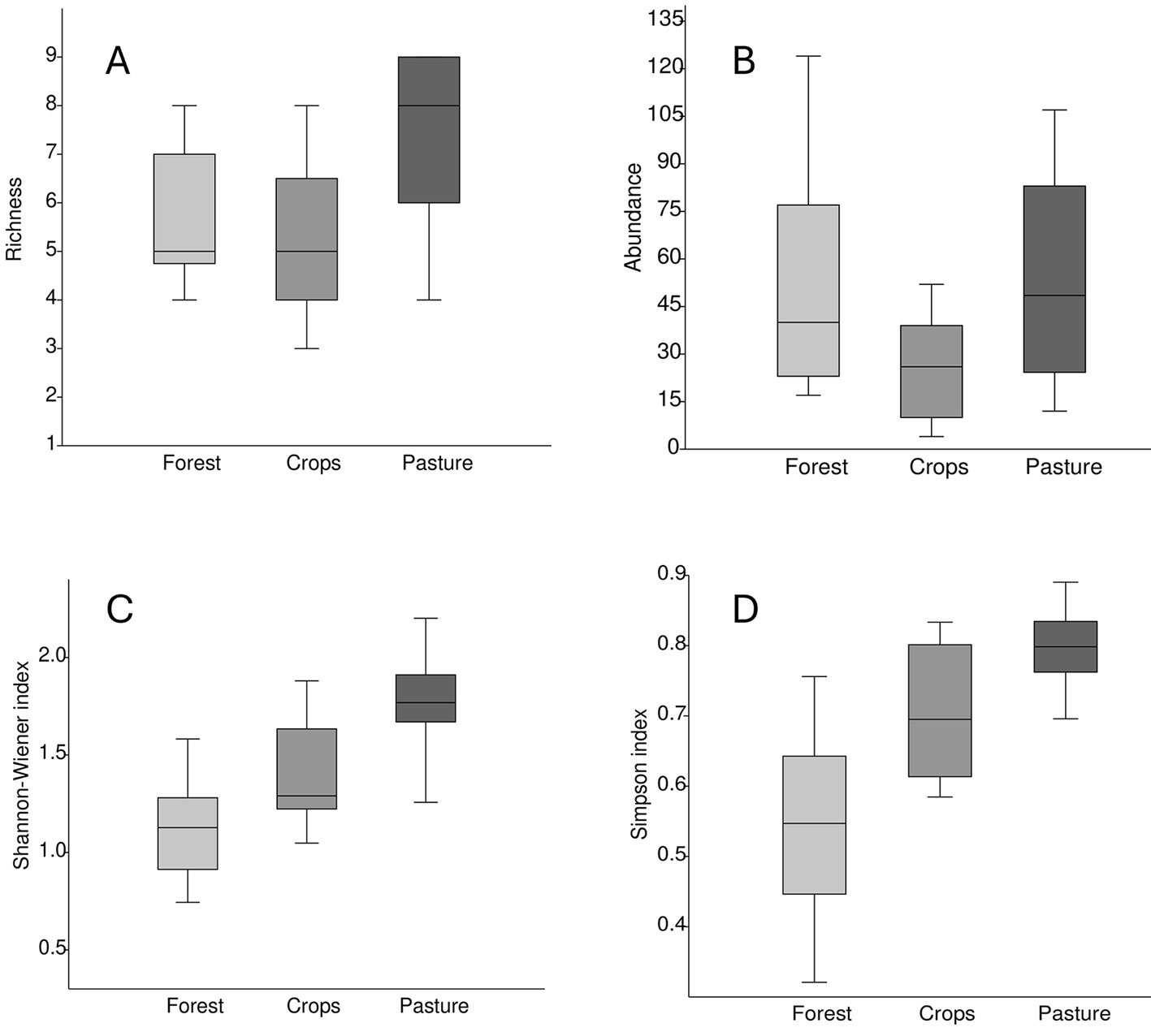
Figure 3. Box plots of richness (A), abundance (B), Shannon Index (C), and Simpson (D) for each of the 3 vegetation covers.

Figure 4. Histogram and box plot of daily ambient temperature across the sampling months; temperature (A, B), rainfall (C).
According to the determined Shannon-Wiener index, the diversity for forest cover was 1,631, crops 1,677, and pasture 2,107. On the other hand, Simpson’s index estimated a dominance of 0.726 for the forest, crops 0.746, and pasture 0.858. When comparing the metrics recorded in each vegetation cover (Fig. 3), the pastures registered on average the greatest richness, abundance, and diversity. The average richness was similar between the crops and the forest; however, the variation was greater in the crops. In contrast, the average and variation of abundance was greater in the forest than in the crops. The average species diversity was lowest in forests, intermediate in crops, and highest in pastures. There were statically differences of all metrics among vegetation cover; richness (one-way ANOVA, F = 5.456, df = 2, p > 0.05), abundance (H(χ2) = 4.63, p > 0.05), Shannon (one-way ANOVA, F = 16.71, df = 2, p > 0.05), and Simpson (H(χ2) = 15.97, p > 0.05).
When we graph the monthly fluctuations of ambient temperature and precipitation (Fig. 4), it is evident that during the days and months of sampling, precipitation was little or none (monthly average from 1.3 mm in January to 7.4 mm in April) whereas monthly average temperature tended to increase from 21.5 °C to 23.3 °C from January to March and from 24.0 to 24.5 °C from April to June. These daily temperature records showed significant monthly differences (ANOVA, F = 67.1, df5 = 5, df2 = 79.8, p < 0.001). There were no significant monthly fluctuations with respect to precipitation (ANOVA, F = 1.78, df5 = 5, df2 = 78.8, p > 0.05). The species richness tended to be higher in April and June in all 3 vegetation covers (Fig. 5) whereas abundance was higher in the forest in March and higher for pastures and crops during April and June. Species diversity (Shannon and Simpson) in the forest was higher in March whereas in both crops and pastures it was higher in June (Fig. 5).
Based on the Jaccard similarity index, crop and pastures presented a greater degree of similarity (Fig. 6), that is, a greater number of shared species. The forest presented the greatest dissimilarity in species composition with respect to the crop and the pasture, having a greater number of unique species (D. truncatus, D. ebraccatus, L. poecilochilus, and L. savagei), which are shown in Table 1.
It was observed that the microhabitat most used by anurans in the forest was leaf litter. The species most associated with this type of microhabitat were D. truncatus and L. poecilochilus (Fig. 7); these species were only recorded in this coverage (Table 1). In the pasture, the highest record of species was found in bare soils and jagüeyes, with L. fuscus, L. insularum, and B. pugnax being the most associated with the latter, while R. horribilis and R. humboldti were observed mainly in bare soil (Fig. 8). In addition, these species presented the highest number of records of individuals in this coverage (Table 1). Finally, in the crop coverage, the microhabitat with the highest number of anuran records was bare soil (Fig. 9), this microhabitat was used most frequently by R. humboldti, R. horribilis, and P. brachyops which were the species with the highest number of individuals recorded; this microhabitat was also used by E. panamensis, which was the only species present in this cover (Table 1).
Discussion
In this study, 19 species of anurans and 1 casual record were identified, for a total of 20 species, this being a slightly smaller number than the 21 species recorded in the SFF Los Colorados 2018-2023 Management Plan (Jiménez et al., 2018). Craugastor raniformis (Boulenger, 1896), Pseudopaludicola pusilla (Ruthven, 1916), and Lectodactylus fragilis (Brocchi, 1877) were not observed in our study, possibly due to lack of sampling in some areas of the SFF Los Colorados. Their occurrence cannot be ruled out, since they were recorded by Acosta-Galvis (2012) in the Montes de María. This study reports C. raniformis in the forest, in ravines (on rocks), on leaf litter, and in shrubby vegetation; P. pusilla in crop areas and on the edge of plain forests, on sandy substrates and in cracks after rains; L. fragilis in flat areas, around seasonal ponds, and near swamps.
Scarthyla, D. ebraccatus, and L. savagei are added to the anuran fauna of the SFF Los Colorados, which shows that it is necessary to continue carrying out studies in the subregions of STDF, including the protected areas of the plains of the Caribbean region, valleys of the Magdalena and Cauca Rivers, Catatumbo, and enclaves of the Patía Valley. Amphibian diversity is poorly known due to the lack of biological studies (Urbina-Cardona et al., 2014).
Sampling carried out in the first 3 months of the year (January, February, and March) regularly corresponds to the dry season (Rangel & Carvajal-Cogollo, 2012). However, rains occurring in these months is a consequence of the effects of the La Niña phenomenon in Colombia for 2022 (Guzmán-Ferraro & García, 2022).
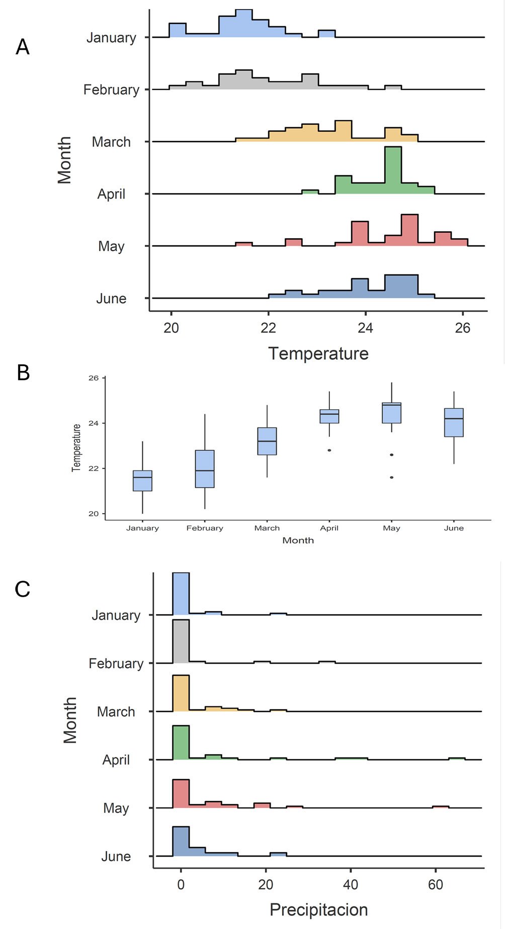
Figure 4. Histogram and box plot of daily ambient temperature across the sampling months; temperature (A, B), rainfall (C).
Increases were observed in the specific richness and in the recorded number of individuals as rainfall increased (especially in April and June), so it was considered that the rainfall regime prior to sampling played an important role in the observation of anurans. These increases in richness and mainly in the number of individuals are attributed to higher activity and the reproductive strategies of some species, which take advantage of the rains to reproduce and lay eggs in temporary ponds. The rains caused greater activity and detectability of some species that were observed vocalizing in small ponds that had formed and cow dams.

Figure 5. Monthly trend of average richness (A), abundance (B), and diversity (C, D) for each vegetation cover type.
Only some amplexuses were recorded but we did not record nesting or reproduction events. Some of the species have explosive activity, which generates an increase in the number of individuals, as is the case of R. horribilis and other species (Vargas-Salinas et al., 2019); some other species vocalizing included Engytomops pustulosus in some ponds and Dendropsophus microcephalus in the emerging vegetation around the cow dams. However, it is worth mentioning that the frequency and intensity of the La Niña phenomenon due to climate change could alter the reproductive times of anurans, causing many species to have early reproduction, which would bring about temporal overlaps of the species that would generate changes in the structure of the assembly (Lawyer & Morin, 1993).
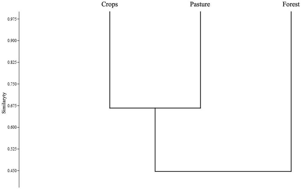
Figure 6. Jaccard similarity dendrogram for the anuran samples from the SFF Los Colorados.
As we expect, there were differences of species richness among vegetation covers. The forest recorded greater richness of anurans than the productive systems (pasture and crops). This is mainly attributed to the greater availability of humid microhabitats and the vegetaion complexity, since there are species that require dense vegetation cover and abundant leaf litter. For example, the oviposition of D. truncatus occurs in humid leaf litter (Cárdenas-Ortega et al., 2019), so different studies record it abundantly in forested areas (Burbano-Yandi et al., 2016; De la Ossa et al., 2016, 2011; Posso-Peláez et al., 2017). On the other hand, pasture and crop are covers with less complexity in the vegetal structure, generating changes in the composition of the anuran assemblages (Cortés-Gómez et al., 2013), such as the reduction in richness, which is closely linked to the reproductive modes of each species (Almeida-Gomes & Rocha, 2015). These same changes in richness in covers with different degrees of disturbance have been recorded in different studies carried out in the Middle Magdalena Valley, in Meta, and in Florencia (Burbano-Yandi et al., 2016; Cáceres-Andrade & Urbina-Cardona, 2009; Duarte-Marín et al., 2018). However, total and monthly average species richness and diversity tended to be higher in the pastures and the lowest in the forests, which registered the greatest monthly variation, recorded the higher species richness and diversity in April and June. The greater diversity of species recorded in pastures may be associated with the lower complexity of the vegetation structure of this habitat, which allows anurans to be easier to detect, while the greater structural complexity of forests and crops decreases detectability of the anurans. Additionally, the presence of jagüeyes in pastures, as sites with availability of water and constant humidity necessary for the survival of the anurans, contributed to the greatest number of records of individuals in this vegetation coverage. Leptodactylus fuscus, L. insularum, and B. pugnax had greater abundance in cow dams of the pasture, since they make postures close to bodies of water (Carvajal-Cogollo et al., 2019; Ortega-Chinquilla et al., 2019).

Figure 7. Use of microhabitats by species in the forest cover of the SFF Los Colorados.
Jagüeyes are considered important for many species in disturbed areas because they permanently provide water resources, which can be used to increase water uptake and reduce evaporation rates (Urbina-Cardona et al., 2014), in addition to be used by species with reproductive modes associated with this resource (Cardozo & Caraballo, 2017). On the other hand, bare soils were mostly used by R. horribilis and R. humboldti, which are species that are commonly found in disturbed areas (Acosta-Galvis, 2012), these have physical characteristics (tuberculated skin) and physiological characteristics that allow them to adapt to exploit this microhabitat (Cáceres-Andrade & Urbina-Cardona, 2009), for this reason, they were found with greater abundance in pastures and crops.
Dendrobates truncatus, D. ebraccatus, L. poecilochilus, and L. savagei are species that were recorded only in the forest, similar to what has been reported by other anuran assemblage studies, where they are not only recorded in forested areas, but also in wetlands (Acosta-Galvis et al., 2006; Angarita et al., 2015; Burbano-Yandi et al., 2016). On the other hand, S. vigilans was only recorded in pastures; in this study the species was observed mainly around bodies of water, specifically on emergent vegetation, in sympatry with D. microcephalus (Muñoz-Guerrero et al., 2007; Fonseca- Pérez et al., 2017). Finally, E. panamensis was only present in crops, although in the study carried out by Blanco-Torres et al. (2015), it was also recorded in pastures. This is a species identified as a leaf miner (Cuentas et al., 2002), which has possibly been the reason why it was observed near the cracks produced by cassava plantations. It is due to all the above that the species similarity analysis showed that the forest differs with respect to the other 2 covers, which are noticeably more similar to each other. Just as we expected, the forest differs in species composition.
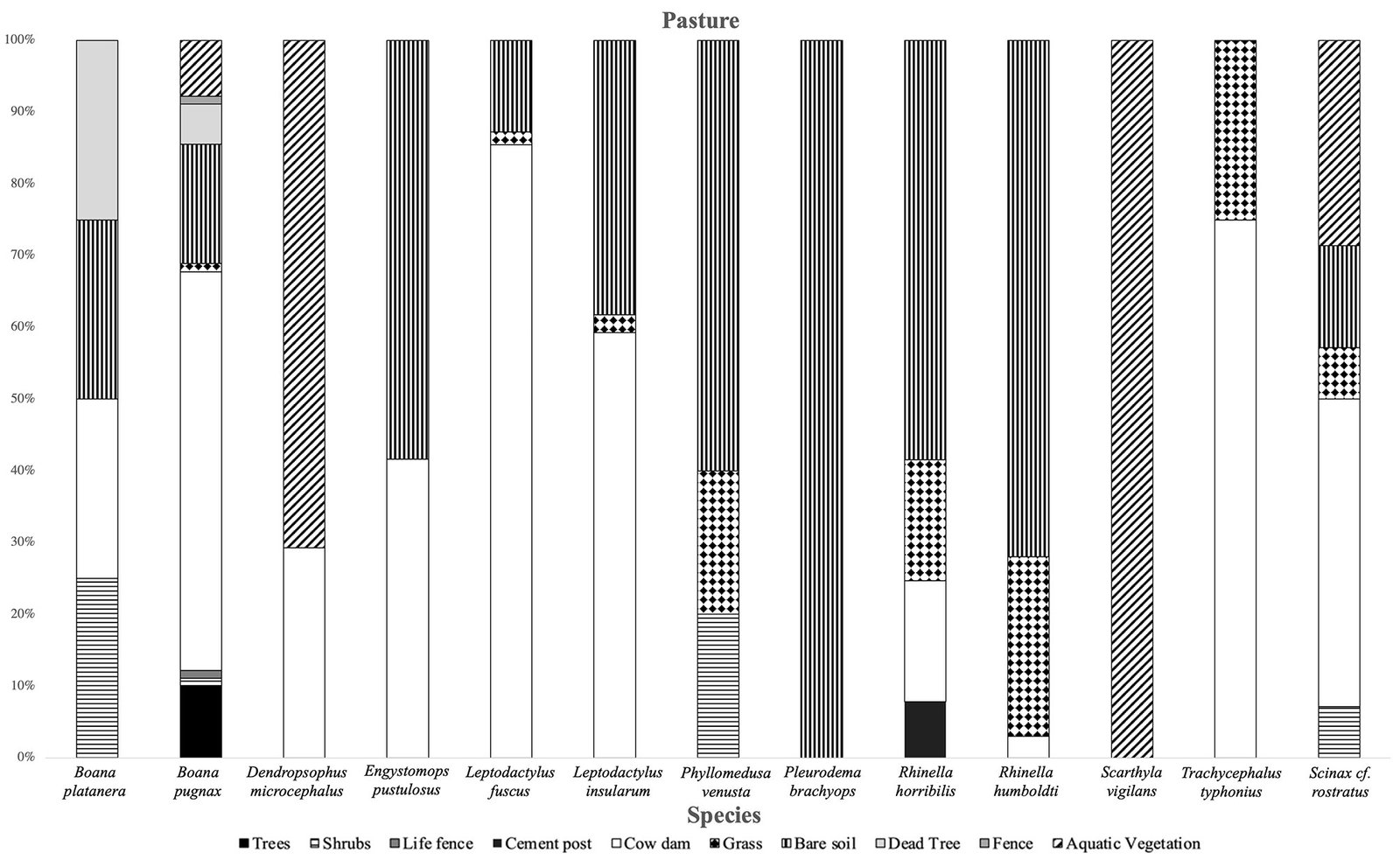
Figure 8. Use of microhabitats by species in the pasture cover of the SFF Los Colorados.
The species diversity index values reported in our study are similar to those obtained in a nearby area located in Meta, Colombia (Cáceres-Andrade and Urbina-Cardona, 2009) where they reported values of 1.4 for humid forest, 1.43 in pastures and 1.9 in sugarcane crops. On the other hand, Román-Palacios et al. (2016) estimated a low Shannon-Wiener index in the Magdalena Medio for forest and quarry (0.92 and 1.74, respectively), while for the lake, they estimated an intermediate diversity (2.03). The forest value was very far from that estimated in this work, which may indicate that the SFF Los Colorados forest has an important conservation status that benefits the anurafauna.
On the other hand, Simpson’s index estimated high dominance for the 3 plant covers. This dominance may be associated with the microhabitats they offer; for example, the forest offered important microhabitats (numerous ponds and abundant leaf litter) for the development of E. pustulosus and D. truncatus, which made these species dominant in this cover. On the other hand, the crop was dominated mainly by P. brachyops, R. humbolbti, and R. horribilis; these species have terrestrial habits, tolerant to landscape transformations and abundant open environments (Acosta-Galvis, 2012; Rodríguez-Molina, 2004). Finally, the pasture was dominated by species of the genus Rhinella and Leptodactylus, where the latter has reproductive modes associated with foam nests, allowing them to conquer and be abundant in anthropized environments (Alcaide et al., 2012).
Jaccard’s similarity analysis for the anurans of the SFF Los Colorados indicates a grouping between pasture and crop cover due to the percentage of shared species (66.6%). This result may be associated with the fact that both covers are intervened areas, with a vegetation structure different from that of the forest and host generalist species (e.g., P. brachyops, B. pugnax, L. fuscus) that can share in greater quantities, while the forest, due to the resources it offers, may have species that do not tolerate landscape transformations (e.g., D. truncatus), being restricted only to forested areas (Cáceres-Andrade & Urbina-Cardona, 2009).

Figure 9. Use of microhabitats by species in the crop cover of the SFF Los Colorados.
The results of this research indicate that the transformation of the landscape because of the agricultural economy of the Montes de María, based mainly on cultivation and the raising of animals (Aguilera-Díaz, 2013), generated changes in the wealth, abundance, composition and use of microhabitats in anuran assemblages. Therefore, this knowledge is important to create concrete tools for the management and conservation of these organisms in the protected area and its surroundings, such as maintaining native vegetation and layers of leaf litter in productive systems, conserving lentic and lotic water sources, and reducing the use of agrochemicals, among others (Urbina-Cardona et al., 2015).
This research constitutes the baseline to evaluate the long-term response of anurans to ecological restoration processes and initiatives led by the SFF Los Colorados team in transformed areas of the protected area. This research constitutes the baseline to evaluate the long-term response of anurans to ecological restoration processes and initiatives led by the SFF Los Colorados team in transformed areas of the protected area. Results that could be useful in future studies where reference ecosystems (conserved areas) and disturbed areas in the process of restoration are used, to determine if these protected areas are achieving the expected objectives and if they are contributing to the conservation of anurans (Urbina-Cardona et al., 2015). Additionally, this study updates the list of anuran species in the protected area, pointing out those to a specific coverage and those shared among covers (forest, pasture, and crops), which can be useful to define those that may be vulnerable to fragmentation of the habitat or to be included as conservation target values (VOC) of the SFF Los Colorados in the construction of future Management Plans.
Acknowledgments
We thank the Hydrobiology research group of the University of Cartagena for providing their equipment for the development of this research. Likewise, to the University of Cartagena, for the financial support through resolution number 01878 of 2022. To IDEAM for providing information on the environmental variables for 2022. To Gabriel R. Navas-S, Dr. Andrés García, and Vivarium del Caribe for financial support and suggestions for carrying out this study. Likewise, to the technical and administrative team of the Los Colorados Flora and Fauna Sanctuary for their support in sampling, logistics, loan of facilities, and management of the research guarantee. To Joselin Castro-Palacios for his support in the implementation of the methodology of this work and to Adolfo A. Mulet-Paso for his suggestions in the identification of the species. To David Gernandt, for his revision to the text which improved substantially.
References
Acosta-Galvis, A. R. (2012). Anfibios de los enclaves secos del área de influencia de los montes de María y la ciénaga de La Caimanera, departamento de Sucre, Colombia. Biota Colombiana, 13, 211–255.
Acosta-Galvis, A. R. (2021). Lista de anfibios de Colombia. BATRACHIA. Retrieved on June 17, 2021 from: http://www.batrachia.com
Acosta-Galvis, A. R., Huertas-Salgado, C., & Rada, M. (2006). Aproximación al conocimiento de los anfibios en una localidad del Magdalena medio (Departamento de Caldas, Colombia). Revista de la Academia Colombiana de Ciencias Exactas, Físicas y Naturales, 30, 291–303. https://doi.org/10.18257/raccefyn.30(115).2006.2250
Acuña-Vargas, J. C. (2016). Anfibios y reptiles asociados a cinco coberturas de la tierra, municipio de Dibulla, La Guajira, Colombia. Acta Zoológica Mexicana, 32,133–146. https://doi.org/10.21829/azm.2016.322940
Aguilera-Díaz, M. M. (2013). Montes de María: una subregión de economía campesina y empresarial. Cartagena: CEER.
Aguirre-León, G. (2011). Métodos de estimación, captura y contención de anfibios y reptiles. Manual de Técnicas para el estudio de la Fauna. In S. López-González y C. López-González (Eds.), Manual de técnicas para el estudio de fauna (pp. 61–85). Querétaro: Universidad Autónoma de Querétaro, A.C.
Alcaide, A. P., Ponssa, M. L., Alcaide, F. P., & Alcaide, M. (2012). Histología de ovario en hembras vitelogénicas de Leptodactylus latinasus (Anura, Leptodactylidae). Acta Zoológica Lilloana, 56, 44–53.
Almeida-Gomes, M., & Rocha, C. F. (2015). Habitat loss reduces the diversity of frog reproductive modes in an Atlantic Forest fragmented landscape. Biotropica, 47, 113–118. https://doi.org/10.1111/btp.12168
Andrade, M. G. (2011). Estado del conocimiento de la biodiversidad en Colombia y sus amenazas. Consideraciones para fortalecer la interacción ciencia-política. Revista de la Academia Colombiana de Ciencias Exactas, Físicas y Naturales, 35, 491–508.
Angarita, M. O., Montes-Correa, A. C., & Renjifo, J. M. (2015). Amphibians and reptiles of an agroforestry system in the Colombian Caribbean. Amphibian and Reptile Conservation, 8, 33–52.
Blanco, A., & Bonilla, M. (2010). Partición de microhábitats entre especies de Bufonidae y Leiuperidae (Amphibia: Anura) en áreas con bosque seco tropical de la región Caribe-Colombia. Acta Biológica Colombiana, 15,47–60.
Blanco-Torres, A., Duré, M., & Bonilla, M. A. (2015). Observaciones sobre la dieta de Elachistocleis pearsei y Elachistocleis panamensis en dos áreas intervenidas de tierras bajas del norte de Colombia. Revista Mexicana de Biodiversidad, 86,538–540. https://doi.org/10.1016/j.rmb.2015.04.031
Ballesteros-Correa, J., Vidal-Pastrana, C., & Ortega-León, A. M. (2019). Anfibios de Córdoba, Colombia. Córdoba: Fondo Editorial de Córdoba.
Burbano-Yandi, C. E., Gómez-Díaz, M. A., Gómez-Figueroa, A., Velásquez-Trujillo, D. A., & Bolívar-García, W. (2016). Ensamblaje de anfibios presentes en un bosque seco y en sistemas productivos, Valle Medio del Magdalena, Victoria y La Dorada, Caldas, Colombia. Revista de Ciencias, 20, 81–93.
Cáceres-Andrade, S. P., & Urbina-Cardona, J. N. (2009). Ensamblajes de Anuros de sistemas productivos y bosques en el Piedemonte Llanero, departamento del Meta, Colombia. Caldasia, 31, 175–195.
Cárdenas-Ortega, M. S., Gutiérrez-Cárdenas, P. D., Cifuentes-Ortegón, M., & Patiño-Gallego, A. M. (2019). Dendrobates truncatus (Cope, 1861) Rana venenosa de rayas amarillas. Catálogo de Anfibios y Reptiles de Colombia, 5, 32–41.
Cardozo, J., & Caraballo, P. (2017). Fauna anura (Amphibia: Anura) asociada a jagüeyes en dos localidades de la región Caribe colombiana. Revista Colombiana de Ciencia Animal-RECIA, 9, 39–47. https://doi.org/10.24188/recia.v9.nS.2017.519
Carvajal-Cogollo, J. E., Bernal-González, V., Paternina-Hernández, A., Muñoz-Ávila, J. N., & Vargas-Salinas, F. (2019). Uso de hábitat y reglas de ensamble: patrones y mecanismos. In M. H. Restrepo-Domínguez, E. Vera-López, Y. Bolívar-Suárez, S. G. Numpaque-Piracoca, O. Y. Acuña-Rodríguez, Z. Z. Ojeda-Pérez et al. (Eds.), Biología de los anfibios y reptiles en bosque tropical del norte de Colombia (pp. 297–338). Tunja: Editorial UPTC.
Clarke, K. R., Gorley, N. R., Somerfield, P. J., & Warwick, R. M. (2014). Change in marine communities: an approach to statistical analysis and interpretation. Plymouth: PRIMER-E.
Colwell, R. K., & Coddington, J. A. (1994). Estimating terrestrial biodiversity through extrapolation. Philosophical Transactions of the Royal Society of London. Series B: Biological Sciences, 345,101–118. https://doi.org/10.1098/rstb.1994.0091
Conell, J. H. (1978). Diversity in tropical rain forests and coral reefs. Science, 199,1302–1310. http://dx.doi.org/10.1126/science.199.4335.1302
Cortés-Gómez, A. M., Castro-Herrera, F., & Urbina-Cardona, J. N. (2013). Small changes in vegetation structure create great changes in amphibian ensembles in the Colombian Pacific rainforest. Tropical Conservation Science, 6, 749–769. https://doi.org/10.1177/194008291300600604
Cortez, F. C., Suárez-Mayorga, A. M., & López-López, F. J. (2006). Preparación y preservación de material científico. In A. Angulo, J. V. Rueda-Almonacid, J. V. Rodríguez-Mahecha y E. La Marca (Eds.), Técnicas de inventario y monitoreo para los anfibios de la región tropical andina (pp. 173–218). Bogotá: Panamericana Formas e Impreso S.A.
Cristal, A., Sánchez, E., Romero, J., Leyva, J., Andrade, W., & Buelvas, C. (2020). ¿Qué hemos logrado con el proyecto de Conectividades Socio-Ecosistémicas? La evolución de la metodología de las 4Ps: avances y retos. In A. Cristal, M. Peña y J. Ferrer-Sotelo (Eds.), El proyecto de conectividades Socio-Ecosistémicas en los Montes de María, 2013–2020 (pp. 63–87). Bogotá-Colombia: Fundación Herencia Ambiental Caribe.
Crump, M., & Scott, N. (2001). Relevamiento por encuentros visuales. In W. R. Heyer, M. A. Donnelly, R. W. Diarmid, L. C. Hayek, & M. S. Foster (Eds.), Medición y monitoreo de la diversidad biológica: métodos estandarizados para anfibios (pp. 80–86). Chubut, Argentina: Editorial Universitaria de la Patagonia.
Cuentas, D., Borja, R., Lynch, J. D., & Renjifo, J. M. (2002). Anuros del departamento del Atlántico y norte de Bolívar. Barranquilla: Editorial Cencys.
De Sá, R. O. (2005). Crisis global de biodiversidad: importancia de la diversidad genética y la extinción de anfibios. Agrociencia, 9, 513.
De la Ossa, J., Contreras-Gutiérrez, J. C., & Campillo-Castro, J. (2011). Censo de Dendrobates truncatus (Anura, Dendrobatidae) en la reserva forestal protectora Serranía de Coraza, Montes de María, Sucre, Colombia. Revista Colombiana de Ciencia Animal-RECIA, 3, 339–343. https://doi.org/10.24188/recia.v3.n2.2011.407
Díaz, S., Fargione, J., Chapin, F. S., & Tilman, D. (2006). Biodiversity loss threatens human well-being. Plos Biology, 4, 1300–1305. https://doi.org/10.1371/journal.pbio.0040277
Duarte-Marín, S., González-Acosta, C., & Vargas-Salinas, F. (2018). Estructura y composición de ensamblajes de anfibios en tres tipos de hábitat en el Parque Nacional Natural Selva de Florencia, Cordillera Central de Colombia. Revista de la Academia Colombiana de Ciencias Exactas, Físicas y Naturales, 42, 227–236. https://doi.org/10.18257/raccefyn.631
Dunn, E. R. (1944). Los géneros de anfibios y reptiles de Colombia. Caldasia, 2,497–529.
Echeverry, M. A., & Rodríguez, J. M. (2006). Análisis de un paisaje fragmentado como herramienta para la conservación de la biodiversidad en áreas de bosque seco y subhúmedo tropical en el municipio de Pereira, Risaralda Colombia. Scientia et Technica, 12, 405–410.
Etter, A., Andrade, A., Saavedra, K., Amaya, P., Cortés, J., Pacheco, C. et al. (2017). Lista Roja de Ecosistemas de Colombia, 2,1–6. https://doi.org/10.13140/RG.2.2.10861.08165
Etter, A., McAlpine, C., & Possingham, H. (2008). Historical patterns and drivers of landscape change in Colombia since 1500: a regionalized spatial approach. Annals of the Association of American Geographers, 98, 2–23. https://doi.org/10.1080/00045600701733911
Fonseca-Pérez, K. A., Molina, C., & Tárano, Z. (2017). Diet of Dendropsophus microcephalus and Scarthyla vigilans (Anura: Hylidae) at a locality in north-western Venezuela with notes on microhabitat occupation. Papéis Avulsos de Zoologia, 57,93–104. https://doi.org/10.11606/0031-1049.2017.57.07
Fox, B. J., Taylor, J. E., Fox, M. D., & Williams, C. (1997). Vegetation changes across edges of rainforest remnants. Biological Conservation, 82, 1–13. https://doi.org/10.1016/S0006-3207(97)00011-6
Galván-Guevara, S., Ballut-Dajud, G., & De La Ossa, J. (2015). Determinación de la fragmentación del bosque seco del arroyo Pechelín, Montes de María, Caribe, Colombia. Biota Colombiana, 16, 149–157.
García, R. J. C., Castro, H. F., & Cárdenas, H. H. (2005). Relación entre la distribución de anuros y variables del hábitat en el sector La Romelia del Parque Nacional Natural Munchique (Cauca, Colombia). Caldasia, 27, 299–310.
García, H., Corzo, G., Isaacs, P., & Etter, A. (2014). Distribución y estado actual de los bosques remanentes del bioma de bosque seco tropical en Colombia: insumos para su gestión. In C. Pizano, & H. García (Eds.), El bosque seco tropical en Colombia (pp. 228–251). Bogotá: Instituto de Investigación de Recursos Biológicos Alexander von Humboldt.
Guzmán-Ferraro, M., & García, G. (2022). El fenómeno de La Niña persistirá hasta casi la mitad del año. CVC. Retrieved on January 14th, 2022 from: http://www.cvc.gov.co/boletin-prensa-007-2022
Hammer, Ø., Harper, D. A., & Ryan, P. D. (2001). PAST: Paleontological statistics software package for education and data analysis. Palaeontologia Electronica, 4, 1–9.
Herazo, F., Mercado, J., & Mendoza, H. (2017). Estructura y composición florística del bosque seco tropical en los Montes de María (Sucre-Colombia). Ciencia en Desarrollo, 8,71–8.
Instituto Alexander von Humboldt. (1998). El bosque seco tropical en Colombia B-sT. Grupo de Exploraciones y Monitoreo Ambiental. Bogotá, Colombia.
IDEAM (Instituto de Hidrología, Meteorología y Estudios Ambientales), IGAC (Instituto Geográfico Agustín Codazzi), & CORMAGDALENA (Corporación Autónoma Regional del río Grande de La Magdalena). (2008). Mapa de cobertura de la Tierra Cuenca Magdalena-Cauca: Metodología CORINE Land Cover adaptada para Colombia a escala 1:100.000. Bogotá: IDEAM/ IGAC/ CORMAGDALENA.
Jiménez, B., De la Rosa, N., & Naranjo, D. (2018). Plan de manejo del Santuario de Flora y Fauna Los Colorados. Parques Nacionales Naturales de Colombia. Santa Marta: Dirección Territorial Caribe.
Laurance, W. F., & Gascon, C. (1997). How to creatively fragment a landscape. Conservation Biology, 11, 577–579.
Lawler, S., & Morin, P. (1993). Temporal overlap, competition, and priority effects in larval anurans. Ecology, 71, 174–182. https://doi.org/10.2307/1939512
Magurran, A. (2004). Measuring biological diversity. Malden: Blackwell Publishing.
Manzanilla, J., & Péfaur, J. E. (2000). Consideraciones sobre métodos y técnicas de campo para el estudio de anfibios y reptiles. Revista de Ecología Latinoamericana, 7,17–30.
Marín, A. M., Ríos, L., Ríos, L., & Almario, J. (2017). Impacto de la actividad ganadera sobre el suelo en Colombia. Ingeniería y Región, 17, 1–12. https://doi.org/10.25054/issn.2216-1325
Meza-Tílvez, K., Mulet-Paso, A., & Zambrano-Cantillo, R. (2018). Fauna del Jardín Botánico de “Guillermo Piñeres” de Cartagena, Turbaco, Colombia: Anfibios y reptiles. Versión 1. Chicago, Illinois: Field Museum.
Moreno, C. E. (2001). Métodos para medir la biodiversidad. Volumen 1. Zaragoza: CYTED, ORCYT/ UNESCO & SEA.
Muñoz-Guerrero, J., Serrano, V. H., & Ramírez-Pinilla, M. P. (2007). Uso de microhábitat, dieta y tiempo de actividad en cuatro especies simpátricas de ranas hílidas neotropicales (Anura: Hylidae). Caldasia, 29, 413–425.
McDiarmid, R. W. (1994). Preparing amphibians as scientific specimens. In W. R. Heyer, M. A. Donnelly, R. W. McDiarmid, L. C. Hayek, & M. S. Foster (Eds.), Measuring and monitoring biological diversity. standard methods for amphibians (pp: 289–296). Washington D.C.: Smithsonian Institution Press.
O’Malley, B. (2007). Anatomía y fisiología clínica de animales exóticos. Zaragoza: Servet.
Ortega-Chinquilla, J., Méndez-Narváez, J., Carvajalino-Fernández, J., & Galindo-Uribe, D. (2019). Ecofisiología. In F. Vargas-Salinas, J.A. Muñoz-Avila & M.E. Morales-Puente (Eds.), Biología de los anfibios y reptiles en bosque tropical del norte de Colombia (pp. 297–338). Tunja: Editorial UPTC.
Pizano, C., Gonzáles, R., Gonzáles, M., Castro-Lima, R., Rodríguez, N., Idárraga, A. et al. (2014). Plantas de los bosques secos de Colombia. In C. Pizano, & H. García (Eds.), El bosque seco tropical en Colombia (pp. 228–251). Bogotá: Instituto de Investigación de Recursos Biológicos Alexander von Humboldt.
Posso-Peláez, C., Blanco-Torres, A., & Gutiérrez-Moreno, L. C. (2017). Uso de microhábitats, actividad diaria y dieta de Dendrobates truncatus (Cope, 1861) (Anura: Dendrobatidae) en bosque seco tropical del norte de Colombia. Acta Zoológica Mexicana, 33, 490–502.
Rangel, C. J. O., & Carvajal-Cogollo, J. E. (2012). Clima de la región Caribe Colombiana. In J. O. Rangel (Ed.), Colombia diversidad biótica XII: la región Caribe de Colombia (pp. 67–129). Bogotá: Instituto de Ciencias Naturales.
Re:wild, Synchronicity Earth, IUCN SSC Amphibian Specialist Group. (2023). State of the World’s Amphibians: The Second Global Amphibian Assessment. Texas: Re:wild. Electronic source at the IUCN website
Rodríguez-Molina, C. R. (2004). Reproducción de Pleurodema brachyops (Anura: Lectodactylidae) en los llanos del Estado Apure, Venezuela. Memoria de la Fundación La Salle Ciencias Naturales, 2002, 117–125.
Rodríguez, G. M., Banda, K., Reyes, S. P., & Estupiñán-González, A. C. (2012). Lista comentada de las plantas vasculares de bosques secos prioritarios para la conservación en los departamentos de Atlántico y Bolívar (Caribe colombiano). Biota Colombiana, 13, 7–39.
Rojas, R. R., & Pérez-Peña, P. E. (2018). Evidencia preliminar del efecto borde en anfibios de la Reserva Nacional Pucacuro, al norte de la Amazonía peruana. Revista del Instituto de Investigaciones de la Amazonía Peruana, 27, 55–67.
Romero, H. G. (2013). Deforestación en Colombia: retos y perspectivas. In F. Dane (Ed.), El desafío del desarrollo sustentable en América Latina (pp. 123–142). Río de Janeiro: SOPLA.
Román-Palacios, C., Fernández-Garzón, S., Hernández, M., Ishida-Castañeda, J., Gallo-Franco, W., & Bolívar-García, A. (2016). Uso de microhábitat por anuros en un fragmento de bosque seco intervenido del Magdalena Medio, Guarinocito, Caldas. Boletín Científico Centro de Museos Museo de Historia Natural, 20, 181–196. https://doi.org/10.17151/bccm.2016.20.2.14
Salvador, J., & Gómez, D. (2018). Reptiles y anfibios del departamento del Atlántico, Colombia. Versión 3. Bogotá, Colombia: Field Museum-Museo de Historia Natural ANDES.
Stuart, S. N., Chanson, J., Cox, N.A., & Young, B. E. (2006). Estado global de los anfibios. In A. Angulo, J. V. Rueda-Almonacid, J. V. Rodríguez-Mahecha, & E. La Marca (Eds.), Técnicas de inventario y monitoreo para los anfibios de la región tropical andina (pp. 19–41). Bogotá: Panamericana Formas e Impreso S.A.
Simmons, J. E., & Muñoz-Saba, Y. (Eds.). (2005). Cuidado, manejo y conservación de las colecciones biológicas. Bogotá: Universidad Nacional de Colombia.
Thompson, P. L., Rayfield, B., & González, A. (2017). Loss of habitat and connectivity erodes species diversity, ecosystem functioning, and stability in metacommunity networks. Ecography, 40, 98–108. https://doi.org/10.1111/ecog.02558
Urbina-Cardona, J. N., Olivares-Pérez, M., & Reynoso, V. H. (2006). Herpetofauna diversity and microenvironment correlates across a pasture-edge-interior ecotone in tropical rainforest fragments in the Los Tuxtlas Biosphere Reserve of Veracruz, Mexico. Biological Conservation, 132,61–75. https://doi.org/10.1016/j.biocon.2006.03.014
Urbina-Cardona, J. N., Arturo-Navas, C., Gonzales, I., Gómez-Martínez., M. J., Llano-Mejía, J., Medina-Rangel, G. F. et al. (2014). Determinantes de la distribución de los anfibios en el bosque seco tropical de Colombia: herramientas para su conservación. In H. Pizano, & H. García (Eds.), El bosque seco tropical en Colombia (pp. 169–195). Bogotá: Instituto de Investigación de Recursos Biológicos Alexander von Humboldt.
Urbina-Cardona, J. N., Bernal, E. A., Giraldo-Echeverry, N., & Echeverry-Alcendra, A. (2015). El monitoreo de herpetofauna en los procesos de restauración ecológica: indicadores y métodos. Monitoreo a procesos de restauración ecológica, aplicado a ecosistemas terrestres. Bogotá: Instituto de Investigación de Recursos Biológicos Alexander von Humbold.
Vargas-Salinas, F., Angarita-Sierra, T., Ospinal, L. A., Rocha-Úsuga, A., & Rueda-Solano, L. (2019). Comunicación y ecología reproductiva. In F. Vargas-Salinas, J.A. Muñoz-Avila & M.E. Morales-Puente (Eds.), Biología de los anfibios y reptiles en bosque tropical del norte de Colombia (pp. 297–338). Tunja: Editorial UPTC.
Vargas, S. F., & Bolaños, L. M. E. (1999). Anfibios y reptiles presentes en hábitats perturbados de selva lluviosa tropical en el bajo Anchicayá, Pacífico colombiano. Revista de la Academia Colombiana de Ciencias Exactas, Físicas y Naturales, 23,499–511.
Villareal, H. M., Álvarez, M., Córdoba-Córdoba, S., Escobar, F., Fagua, G., Gast, F. et al. (2004). Manual de métodos para el desarrollo de inventarios de biodiversidad. Bogotá: Instituto de Investigación de Recursos Biológicos Alexander von Humboldt.
Zug, G. R., Vitt, L., & Caldwell, J. P. (2001). Herpetology: an introductory biology of amphibians and reptiles. San Diego: Academic Press.

Association of Myianoetus sp. (Acari: Histiostomatidae) with necrophagous fly Compsomyiops fulvicrura (Diptera: Calliphoridae), in the Prepuna ecoregion (Jujuy: Argentina)
María Laura Fernández-Salinas a, *, Marcia Luciana Matoz-Fernández b
a Universidad Nacional de Jujuy, Instituto de Biología de la Altura, Avenida Bolivia 1661, 4600 San Salvador de Jujuy, Jujuy, Argentina
b Universidad Nacional de Mar del Plata, Laboratorio de Zoonosis Parasitarias, Funes 3350, 7600 Mar del Plata, Buenos Aires, Argentina
*Corresponding author: mfernandez@inbial.unju.edu.ar (M.L. Fernández-Salinas)
Received: 31 January 2024; accepted: 10 June 2024
Abstract
The genus Myianoetus Oudemans(Acari: Histiostomatidae) is commonly associated with carrion, utilizing flies (Diptera) from various families as a means of dispersal through phoresy. The objective of this paper is to present a new association between Myianoetus sp. mites and Calliphoridae flies and discuss its relevance in forensic sciences. Samples were collected in 3 locations in the Prepuna ecoregion of Jujuy, Argentina. Specimens were captured using necrotraps baited with cow lung. Flies carrying phoretic mites were separated and identified to a specific level, while mites were counted and identified at the lowest possible taxonomic level. Compsomyiops fulvicrura (Robineau-Desvoidy) (Diptera: Calliphoridae) was the only species that presented attached mites, with an average intensity of 12.26 mites per fly. The mites carried by C. fulvicrura were identified as deutonymphs of Myianoetus sp., with a prevalence of 2.56% of infested flies. Significant differences in the abundance of flies with mites were observed between locations and seasons. This article represents the first contribution to knowledge on the specific association between Myianoetus sp. and C. fulvicrura. These findings in forensic ecology are relevant for their potential contribution and application in the development of more precise methods in specific forensic cases.
Keywords: Astigmata; Diptera; Forensic Acarology; Phoresy; New report
© 2024 Universidad Nacional Autónoma de México, Instituto de Biología. Este es un artículo Open Access bajo la licencia CC BY-NC-ND
(http://creativecommons.org/licenses/by-nc-nd/4.0/).
Asociación de Myianoetus sp. (Acari: Histiostomatidae) con la mosca necrófaga Compsomyiops fulvicrura (Diptera: Calliphoridae), en la ecoregión Prepuna (Jujuy: Argentina)
Resumen
El género Myianoetus Oudemans (Acari: Histiostomatidae) suele asociarse a la carroña utilizando moscas (Diptera) de distintas familias como medio de dispersión, a través de la foresia. El objetivo de este trabajo fue presentar una nueva asociación entre Myianoetus sp. con moscas Calliphoridae y discutir su alcance dentro de las ciencias forenses. Las muestras se recolectaron en 3 localidades de la Prepuna jujeña, Jujuy, Argentina. Los especímenes se capturaron mediante necrotrampas cebadas con pulmón vacuno. Las moscas con ácaros se separaron y determinaron a nivel específico; los ácaros fueron numerados e identificados al nivel taxonómico más bajo posible. Compsomyiops fulvicrura (Diptera: Calliphoridae) fue la única especie que presentó ácaros adheridos, con una intensidad media de 12.26 ácaros por mosca. Los ácaros fueron identificados como deutoninfas de Myianoetus sp. y se determinó una prevalencia de 2.56% de moscas infestadas. Se observaron diferencias significativas en la abundancia de moscas con ácaros entre las localidades y estaciones analizadas. Este artículo representa el primer aporte al conocimiento sobre la asociación específica entre Myianoetus sp. y C. fulvicrura. Estos hallazgos sobre ecología forense son relevantes por su potencial contribución y aplicación al desarrollo de métodos más precisos en casos forenses determinados.
Palabras clave:Astigmata; Diptera; Acarología forense; Foresia; Nuevo reporte
Introduction
Carcasses present limited and ephemeral biocenosis made up of diverse organisms that often comprise complex food webs (Braig & Perotti, 2009; Perotti et al., 2010). Many Diptera species actively participate in the cadaveric decomposition process in which the Calliphoridae and Sarcophagidae families, along with Coleoptera are often investigated because of their large number, persistence and capacity to act as hosts to diverse mites that use them for dispersion by phoresis (Camerick, 2010; Perotti & Braig, 2009; Perotti et al., 2010).
Mites present morphological and physiological adaptations to serve phoresy during adult and nymphal stages. These adaptations are documented in the order Mesostigmata, in the suborder Prostigmata and in the infraorder Astigmatina (Oribatida) (Perotti et al., 2010). Astigmata mites are specialists in irregular or ephemeral habitats which they colonize through a deutonymphal heteromorphic stage known as hypopus which is specialized for phoresy (OConnor, 2009). Astigmatid deutonymphs are morphologically simplified, have lost the mouth and chelicerae, have greatly reduced the remainder of the gnathosoma, and have suckers on the paraproctal region for efficient phoretic attachment. The body is strongly dorsoventrally flattened, heavily sclerotized and much more resistant to desiccation than other stages of the life cycle (Farish & Axtell, 1971; OConnor, 1982). The conditions needed to reach this stage may involve genetic factors and physicochemical factors from the environment (Greenberg & Carpenter, 1960).
Astigmatid mites are particularly important for the 3 areas of forensic entomology: urban, stored product pests and medico-legal (Catts & Goff, 1992; Perotti & Braig, 2019). Nevertheless, they often go unnoticed because of their small size. Moreover, their analysis is limited because of difficulties in species identification, lack of specific knowledge and misuse of forensic methodology (OConnor, 2009; Perotti et al., 2010). Numerous species of mites are compulsory or facultative inhabitants of carrion. They are found not only in legal cases that involve human carcasses (Pimsler et al., 2016; Rai et al., 2020; Russell et al., 2004; Saloña-Bordas & Perotti, 2015); but also, in experimental studies concerning faunal succession in animal remains (Arnaldos et al., 2005; Barton et al., 2014; Centeno & Perotti, 1999; Heo et al., 2021).
In Argentina, the only record of the presence of phoretic mites associated with decomposing remains were the preliminary observations of Centeno and Perotti (1999), in which they found mites of the genus Myianoetus Oudemans (Astigmata: Histiostomatidae) associated with a specimen of Morellia sp. (Muscidae). In order to contribute to the further study on phoretic relations between mites and arthropods, this paper presents a new association between mites and Diptera from the Calliphoridae family in Prepuna of Jujuy, Argentina, and discusses its relevance and importance within the forensic sciences.
Materials and methods
The collection of Diptera specimens was carried out in the following locations: Tres Cruces (22°55’06.01” S, 65°35’13.58” W), Humahuaca (23°12’14.27” S, 65°20’54.90” W), and Tumbaya (23°51’27.79” S, 68°28’03.31” W) (Fig. 1a-c). These locations are part of the Monte Province, Prepuna District in the province of Jujuy, Argentina. Two sampling campaigns were carried out, one during the dry season (June, July, and August) and the other during the wet season (December, January, and February) between 2016 and 2018. Each location was equipped with 18 traps, totaling 54 traps across all sampling locations, totaling 108 traps per year.
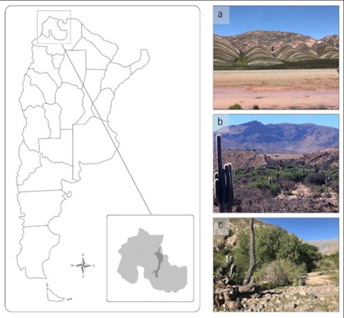
Figure 1. Location of the study area. The map depicts the region corresponding to the Monte Province, Prepuna District, in the province of Jujuy, Argentina. Study sites are located in the following localities: a) Tres Cruces, b) Humahuaca, and c) Tumbaya (Photos by Fernández Salinas, M. L.).
To obtain specimens in good condition for identification, traps were made following Hwang and Turner (2005) (Fig. 2). A modified cone trap, based on a soft drink bottle with a baited target, was constructed. The bottle traps were assembled using two 3 L clear plastic soft drink bottles with a diameter of 11.5 cm, along with a black acrylic container 11 cm measured in diameter and 13 cm in depth. Consisted of 2 parts, the upper collection chamber and the lower bait chamber. The collection chamber was formed from the bottles cut 24 cm and 12 cm from the top respectively, one pushed inside the other (so that the bottle’s spout acts as a funnel and prevents flies from escaping). The bait chamber was made with a black container so the flies were drawn upwards, into the transparent collection chamber. The 2 halves of the trap were push-fitted together and secured by strips of waterproof adhesive tape. To facilitate the entry of flies 4 holes of approximately 0.8 cm in diameter were made around the bait chamber. A 125 cm³ plastic container with the bait was placed at the base of this container. A feeding substrate made of 100 g of cow’s lung was used. A distance of approximately 100 m was maintained between the traps because of the competitive nature of the colonizing species and were separated from the floor as they were hung at a minimum height of 1.5 m to avoid the attack of scavenger mammals. It was placed in a closed recipient which was subjected to a warm temperature between 15 °C and 30 °C, during 60 hours, for sufficient time to decompose. The traps were left in place for 7 consecutive days.
The captured specimens were put in Kahn tubes with 70% alcohol and they were transported to the Institute of Altitude Biology (INBIAL), San Salvador de Jujuy, Jujuy, Argentina.

Figure 2. Design of the bottle necrotrap baited with cow lung.
Flies that presented mites were counted, separated by sex and identified to its most specific level using keys and revisions from Olea and Mariluis (2013), Whitworth (2014), and Mulieri et al. (2014). The flies were photographed “in situ” using a Canon 5D Mark IV camera, 3 extension tubes for macro photography and a Canon 85 mm 1.8 lens illuminated with a Godox AD200 flash and a Godox V860 flash. Afterward, the specimens were sent to the Parasitic Zoonoses Laboratory, National University of Mar del Plata, Mar del Plata, Buenos Aires, Argentina. Each fly was individually examined, and the number of mites per fly and their attachment sites on the host flies were determined. The mites were then removed with the assistance of fine-tipped needles. From selected mite specimens, permanent preparations in Hoyer’s medium were made. The remaining specimens were identified from temporary preparations after being cleared in lactic acid using an open slide technique in order to be observed under the optic microscope (Olympus CX31). Taxonomic identification was done at a genus level using diagnostic keys (Dindal, 1990). Mites were photographed with a Sony Powershot DSC-P200 camera. The photographs were edited with Adobe Photoshop CS.
Table 1
Percentage of prevalence and mean intensity of Myianoetus sp. associated with Compsomyiops fulvicrura, in 3 locations of Jujuy, Argentina.
| Location | Season | Nº of flies with attached mites | Total Nº of flies | Nº of mites | Prevalence (%) | Mean Intensity |
| Tumbaya | Dry | 26 | 661 | 243 | 3.93 | 9.34 |
| Wet | 0 | 85 | 0 | 0 | 0 | |
| Humahuaca | Dry | 40 | 1,517 | 478 | 2.63 | 11.95 |
| Wet | 0 | 205 | 0 | 0 | 0 | |
| Tres Cruces | Dry | 18 | 624 | 156 | 2.88 | 8.83 |
| Wet | 10 | 582 | 276 | 1.71 | 27.3 |
The abundance of flies with attached mites was analyzed using Generalized Linear Models (GLM) through the software InfoStat (Di Rienzo et al., 2020). In the model, the 3 study locations were considered as fixed effects while the seasons were treated as random variables. Variance heterogeneity was adjusted using the VarExp variance function, and models were selected according to Akaike (AIC) and Bayesian (BIC) criteria. Subsequently, a Fisher’s LSD test (α = 0.05) of adjusted means and standard errors was conducted to evaluate differences between locations, following the methods described. Prevalence and mean intensity were calculated as indicated by Bush et al. (1997) and Margolis et al. (1982). Prevalence was calculated as the number of flies infected with phoretic mites, divided by the number of flies examined in a sample, and was expressed as a percentage. The mean intensity of phoresy was defined as the total number of phoretic mites of a particular species found in a sample, divided by the number of host flies.
For further taxonomic studies, voucher species were deposited as slide-mounted specimens in the Entomological Collection “Dr. Lilia Estela Neder”, Institute of Altitude Biology (INBIAL), National University of Jujuy, Jujuy, Argentina (INBIAL C 15000; INBIAL C 15001).
Results
A total of 9,454 Calliphoridae individuals were collected. They spanned 5 genera and 12 species: Calli-
phora vicina (Robineau-Desvoidy), Chlorobrachycoma versicolor (Bigot), Chrysomya albiceps (Wiedemann), Chrysomya megacephala (Fabricius), Cochliomyia mace-llaria (Fabricius), Cochliomya hominiborax (Coquerel), Compsomyiops fulvicrura (Robineau-Desvoidy), Com-psomyiops sp., Lucilia cuprina (Wiedemann), Lucilia sericata (Meigen), Sarconesia chlorogaster (Wiedemann), Sarconesiopsis magellanica (Le Guillou). The most abundant species were C. albiceps and C. fulvicrura with 4,651and 3,674 individuals respectively. C. fulvicrura was the only species that had mites attached to its body (Fig. 3). These mites primarily attached themselves to the thorax and head regions and were identified as deutonymphs of Myianoetus sp. (Figs. 4, 5, 6). The individuals found exhibit morphological similarities to the deutonymphs of Myianoetus muscarum (Linnaeus) (OConnor et al., 2015). However, they differ from this species by possessing dorsal hysterosomal setae of approximately equal length to the exobothridial setae, unlike M. muscarum, where the hysterosomal setae are less than half the length of the exobothridial setae. Given that this characteristic is diagnostic of M. muscarum, we hypothesize that the specimens uncovered in this study may represent a yet undescribed species. Out of the total number of C. fulvicrura individuals, 94 carried phoretic mites (83 females and 11 males), representing a prevalence of 2.56% (Table 1). A total of 1,153 mites were counted, which corresponds to a mean intensity of 12.26 mites/fly (1-89 rank) (Fig. 7). The majority of mites (76%) were found during the dry season in all 3 studied locations. However, in Tres Cruces, mites were also found during the wet season (Table 1).
Table 2
Summary of generalized linear model (GLM) analysis results and model fitting parameters. Significance levels (p values) and variance function parameters, model fitting parameters including number of observations (N), Akaike information criterion (AIC), Bayesian information criterion (BIC), the log probability, the standard deviation (Sigma) and the coefficient of determination (R2) are shown.
| Effects | p-value | Variance function parameters |
| Location | < 0.0001 ** | |
| Season | 0.0105 * | -0.27 (dry) |
| -0.09 (wet) |
Model tuning: N = 6, AIC = 31.83, BIC = 22.68, LogLik = -8.91, Sigma = 4.82, R2 = 0.74
Table 3
Results of the Fisher’s LSD test (α = 0.05): adjusted means and standard errors for the 3 locations under study. Common letters indicate that the means do not differ significantly (p > 0.05).
| Location | Means | SE | |
| Humahuaca | 20.84 | 1.98 | A |
| Tumbaya | 6.84 | 1.98 | B |
| Tres Cruces | 1.16 | 1.98 | C |
The GLM analysis revealed significant differences in the abundance of flies with attached mites among the study locations (p < 0.0001) and a significant effect of seasonality (p = 0.0105) (Table 2).
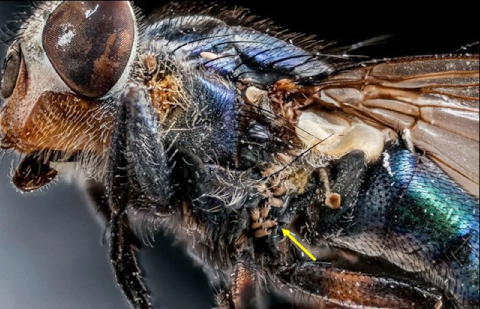
Figure 3. Deutonymphs of Myianoetus sp. (yellow arrow) between the thorax and abdomen of Compsomyiops fulvicrura.
Additionally, subsequent Fisher’s LSD analysis revealed statistically different groups among the study locations. A higher mean abundance of flies with attached mites was observed in Humahuaca, followed by Tumbaya and Tres Cruces (Table 3). It is noteworthy that the highest variance parameter for the dry season (-0.27) compared to the wet season (-0.09) suggests that these differences are primarily attributed to this time of the year, between June and August.

Discussion
The genus Myianoetus comprises more than 40 species widespread throughout the world (OConnor et al., 2015), most known only from deutonymphs phoretic on Diptera. In this work, the association between deutonymphs of Myianoetus sp. with C. fulvicrura is described for the first time. Up to present, there are reports of deutonymphs from the Myianoetus that have been found associated with various Diptera families: Sphaeroceridae (Fain et al., 1980), Muscidae (Centeno & Perotti, 1999; Greenberg & Carpenter 1960; Negm & Alatawi, 2011; Pimsler et al., 2016), Calliphoridae (Greenberg & Carpenter 1960; Miranda & Bermúdez, 2008) and Heleomyzidae (Zamec & Košel, 2014). Evidence obtained from lab experiments further described the phoretic interaction of the hypopi of Myianoetus muscarum with Muscina stabulans Fallen (Diptera: Muscidae), Stomoxys calcitrans Linnaeus (Diptera: Muscidae), Lucilia sericata (Diptera: Calliphoridae) and Musca domestica Linnaeus (Diptera: Muscidae) (Greenberg & Carpenter, 1960). Additionally, in a study carried out in Texas, USA, by Pimsler et al. (2016), a great number of M. muscarum individuals associated with Synthesiomyia nudiseta (Wulp) (Diptera: Muscidae) were collected in 3 human corpses.
Among the Calliphoridae species collected, C. albiceps stood out as the most abundant. However, deutonymphs of Myianoetus sp. were exclusively phoretically associated with C. fulvicrura. The statistical differences observed in the abundances of flies with attached mites among the different studied locations suggest that these were influenced by the dry season. Therefore, the preference for C. fulvicrura could be associated with seasonal variation, as it was more abundant during the dry season, contrasting with C. albiceps, which showed a preference for the wet season. These trends were notable in Tumbaya and Humahuaca, where C. albiceps was the dominant species, while in Tres Cruces, the abundance of this species was very low, with C. fulvicrura being the dominant species in both seasons in that area. Additionally, it is plausible that this choice is related to the chemical attraction of mites to volatile substances released by the puparia of C. fulvicrura, as demonstrated in the studies by Greenberg and Carpenter (1960). These observations were reflected in the prevalence values, which indicated higher values during the dry season in all 3 locations, compared to the wet season.

Figure 5. Dorsal view of Myianoetus sp. (scale = 0.05 mm). The yellow arrow indicates the hysterosomal setae (ex) and exobothridial setae (in).

Figure 6. Dorsal view of legs I and II of Myianoetus sp. (scale = 0.1 mm). The yellow arrow shows the bifurcate empodial claw, characteristic of the genus, present on legs I-III.

Figure 7. Abundance frequency (AF) histogram of Myianoetus sp. deutonymphs associated with Compsomyiops fulvicrura individuals.
The lack of interaction between Myianoetus sp. with other species and its demonstrated affinity with C. fulvicrura suggest that these mites can be phoretically selective in the Prepuna environment. At genus or species level, mites have micro-habitat specific requirements, being excellent specific environmental indicators, offering themselves as potentially one of the most informative pieces of biological trace evidence collected from a crime scene (Perotti & Braig, 2019). This may explain events of corpse location, of relocation, a link to a suspect and a possible connection between a suspect and a victim or a crime scene (Hani et al., 2018; Kamaruzaman et al., 2018; Szeleczl et al., 2018). The specificity and abundance of mites, coupled with the intensity of phoresy, could contribute to estimating more precise post-mortem intervals (PMI) (Miranda & Bermúdez, 2008; Rodrigueiro & Prado, 2004; Russell et al., 2004). In addition, Perotti and Braig (2009) suggested that the presence of a specific phoretic mite (for example Myianoetus sp.) may confirm the presence of its host (for example C. fulvicrura), even when the host is already gone.
Given that mites are a valuable forensic tool, it is crucial to deepen the understanding of the biology and ecology of the species involved. To expand this knowledge, it is necessary to continue registering and investigating new species and their phoretic associations under various climatic and biogeographical conditions.
Acknowledgements
We would like to thank Pablo A. Martínez for his critical analysis and recommendations for our manuscript, Mario A. Linares for the Myianoetus sp.photograph and Ismael Acosta for the C. fulvicrura photograph.
References
Arnaldos, M. I., García, M. D., Romera, E., Presa, J. J., & Luna, A. (2005). Estimation of post-mortem interval in real cases based on experimentally obtained entomological evidence. Forensic Science International, 149, 57–65. https://doi.org/10.1016/j.forsciint.2004.04.087
Barton, P. S., Weaver, H. J., & Manning, A. D. (2014). Contrasting diversity dynamics of phoretic mites and beetles associated with vertebrate carrion. Experimental and Applied Acarology, 63, 1–13. https://doi.org/10.1007/s10493-013-9758-7
Braig, H. R., & Perotti, M. A. (2009). Carcasses and mites. Experimental and Applied Acarology, 49, 45–84. https://doi.org/10.1007/s10493-009-9287-6
Bush, A. O., Lafferty, K. D., Lotz, J. M., & Shostak, A. W. (1997). Parasitology Meets Ecology on Its Own Terms: Margolis et al. Revisited. The Journal of Parasitology, 83, 575–583. https://doi.org/10.2307/3284227
Camerik, A. M. (2010). Phoresy revisited. In M. Sabelis, & J. Bruin (Eds.), Trends in Acarology (pp. 333–336). Dordrecht: Springer. https://doi.org/10.1007/978-90-481-9837-5_53
Catts, E. P., & Goff, M. L. (1992). Forensic entomology in criminal investigations. Annual Review of Entomology, 37, 253–272. https://doi.org/10.1146/annurev.en.37.010192.001345
Centeno, N. D., & Perotti, M. A. (1999). Ácaros vinculados a procesos de descomposición de cadáveres y sus posibles asociaciones foréticas. In Actas y Trabajos de la XIX Reunión Argentina de Ecología, 1999. Tucumán, Argentina.
Di Rienzo J. A., Casanoves, F., Balzarini, M. G., González, L., Tablada, M., & Robledo, C. W. (2020). InfoStat versión 2020. Centro de Transferencia InfoStat, FCA, Universidad Nacional de Córdoba, Argentina.
Dindal, D. L. (1990). Soil biology guide. New York: John Wiley and Sons.
Fain, A., Britt, D. P., & Molyneux, D. H. (1980). Myianoetus copromyzae sp. nov. (Acari, Astigmata, Anoetidae) phoretic on Copromyza atra (Meigen 1830) in Scotland. Journal of Natural History, 14, 401–403. https://doi.org/
10.1080/00222938000770341
Farish, D. J., & Axtell, R. C. (1971). Phoresy redefined and examined in Macrocheles muscaedomesticae (Acarina: Macrochelidae). Acarologia, 13, 16–29.
Greenberg, B., & Carpenter, P. D. (1960). Factors in phoretic association of a mite and fly. Science, 132, 738–739. https://doi.org/10.1126/science.132.3429.738
Hani, M., Thieven, U., & Perotti, M. A. (2018). Soil bulb mites as trace evidence for the location of buried money. Forensic Science International, 292, e25–e30. https://doi.org/10.1016/j.forsciint.2018.09.016
Heo, C. C., Teel, P. D., & OConnor, B. M. (2021). Acari community in association with delayed pig carrion decomposition. Experimental and Applied Acarology, 85, 223–246. https://doi.org/10.1007/s10493-021-00676-6
Hwang, C., & Turner, B. D. (2005). Spatial and temporal variability of necrophagous Diptera from urban to rural areas. Medical and Veterinary Entomology, 19, 379–391. https://doi.org/10.1111/j.1365-2915.2005.00583.x
Kamaruzaman, N. A. C., Mašán, P., Velásquez, Y., González-Medina, A., Lindström, A., Braig, H. R. et al. (2018). Macrocheles species (Acari: Macrochelidae) associated with human corpses in Europe. Experimental and Applied Acarology, 76, 453–471. https://doi.org/10.1007/s10493-018-0321-4
Margolis, L., Esch, G. W., Holmes, J. C., Kuris, A. M., & Schad, G. A. (1982). The use of ecological terms in parasitology (report of an ad hoc committee of the American Society of Parasitologists). Journal of Parasitology, 68, 131–133. https://doi.org/10.2307/3281335
Miranda, R., & Bermúdez, S. (2008). Ácaros (Arachnida: Acari) asociados con moscas Calliphoridae (Diptera: Oestroidea) en tres localidades de Panamá. Revista Colombiana de Entomología, 34, 192–196. https://doi.org/10.25100/socolen.v34i2.9287
Mulieri, P. R., Mariluis, J. C., & Patitucci, L. D. (2014). Calliphoridae. In S. Roig-Juñent, L. E. Claps, & J. J. Morrone (Eds.), Biodiversidad de artrópodos argentinos, Vol. 4 (pp. 463–474). INSUE, Universidad Nacional de Tucumán, San Miguel de Tucumán, Argentina.
Negm, M. W., & Alatawi, F. J. (2011). Four new records of mites (Acari: Astigmata) phoretic on insects in Riyadh, Saudi Arabia. Journal of the Saudi Society of Agricultural Sciences, 10, 95–99. https://doi.org/10.1016/j.jssas.2011.04.001
OConnor, B. M. (1982). Evolutionary ecology of astigmatid mites. Annual Review of Entomology, 27, 385–409. https://doi.org/10.1146/annurev.en.27.010182.002125
OConnor, B. M. (2009). Astigmatid mites (Acari: Sarcoptiformes) of forensic interest. Experimental and Applied Acarology, 49, 125–133. https://doi.org/10.1007/s10493-009-9270-2
OConnor, B. M., Pimsler, M. L., Owings, C. G., & Tomberlin, J. K. (2015). Redescription of Myianoetus muscarum (Acari: Histiostomatidae) associated with human remains in Texas, USA, with designation of a neotype from Western Europe. Journal of Medical. Entomology, 52, 539–550. https://doi.org/10.1093/jme/tjv045
Olea, S. M., & Mariluis, J. C. (2013). The genus Calliphora (Diptera: Calliphoridae) in Argentina, with the first records of C. lopesi Mello 1962. Revista de la Sociedad Entomológica Argentina, 72, 99–104.
Perotti, M. A., & Braig, H. R. (2009). Phoretic mites associated with animal and human decomposition. Experimental and Applied Acarology, 49, 85–124. https://doi.org/10.1007/s10493-009-9280-0
Perotti, M. A., Braig, H. R., & Goff, M. L. (2010). Phoretic mites and carcasses: Acari transported by organisms associated with animal and human decomposition. In J. Amendt, M. Goff, C. Campobasso, & M. Grassberger (Eds.), Current concepts in forensic Entomology (pp. 69–91). Dordrecht: Springer. https://doi.org/10.1007/978-1-4020-9684-6_5
Perotti, M. A., & Braig, H. R. (2019). Acarology in Crimino-Legal Investigations. In J. Byrd, & J. Tomberlin (Eds.), Forensic Entomology, 3rd. Edition (pp. 461–473). Boca Raton: CRC Press. https://doi.org/10.4324/9781351163767-22
Pimsler, M. L., Owings, C. G., Sanford, M. R., OConnor, B. M., Teel, P. D., Mohr, R. M., & Tomberlin, J. K. (2016). Associa-
tion of Myianoetus muscarum (Acari: Histiostomatidae) with Synthesiomyia nudiseta (Wulp) (Diptera: Muscidae) on human remains. Journal of Medical Entomology, 53, 290–295. https://doi.org/10.1093/jme/tjv203
Rai, J., Amendt, J., Bernhardt, V., Pasquerault, T., Lindström, A., & Perotti, M. A. (2020). Mites (Acari) as a relevant tool in trace evidence and postmortem analyses of buried corpses. Journal of Forensic Sciences, 65, 2174–2183. https://doi.org/10.1111/1556-4029.14506
Rodrigueiro, T. S. C., & Prado, A. P. (2004). Macrocheles muscaedomesticae (Acari, Macrochelidae) and a species of Uroseius (Acari, Polyaspididae) phoretic on Musca domestica (Diptera, Muscidae): effects on dispersal and colonization of poultry manure. Iheringia. Série Zoologia, 94, 181–185. https://doi.org/10.1590/S0073-47212004000200011
Russell, D. J., Schulz, M. M., & OConnor, B. M. (2004). Mass occurrence of astigmatid mites on human remains. Abhandlungen und Berichte des Naturkundmuseums Görlitz, 76, 51–56.
Saloña-Bordas, M. I., & Perotti, M. A. (2015). Acarología forense. Ciencia Forense, 12, 91–112.
Szelecz, I., Lösch, S., Seppey, C. V. W., Lara, E., Singer, D., Sorge, F. et al. (2018). Comparative analysis of bones, mites, soil chemistry, nematodes and soil micro-eukaryotes from a suspected homicide to estimate the post-mortem interval. Scientific Reports, 8, 25. https://doi.org/10.1038/s41598-017-18179-z
Whitworth, T. (2014). A revision of the Neotropical species of Lucilia Robineau- Desvoidy (Diptera: Calliphoridae). Zootaxa, 3810, 1–76. https://doi.org/10.11646/zootaxa.3810.
1.1
Zamec, R., & Košel, V. (2014). A new species of mite (Acari: Histiostomatidae) phoretic on Gymnomus caesius (Diptera: Heleomyzidae) from Vlčie Diery cave. Biologia, 69, 916–919. https://doi.org/10.2478/s11756-014-0387-3

Ringtails (Bassariscus astutus) as seed dispersers in an urban gradient under conditions of low human activity due to COVID-19
Joselin Judith Peña-Herrera a, Yury Glebskiy a, b, *, Teresa de Jesús Hernández-Trejo a, Zenón Cano-Santana a
a Universidad Nacional Autónoma de México, Facultad de Ciencias, Departamento de Ecología y Recursos Naturales, Laboratorio de Interacciones y Procesos Ecológicos, Circuito Exterior s/n, Ciudad Universitaria, Coyoacán, 04510 Ciudad de México, Mexico
b Universidad Nacional Autónoma de México, Facultad de Ciencias, Posgrado en Ciencias Biológicas, Circuito Exterior s/n, Ciudad Universitaria, Coyoacán, 04510 Ciudad de México, Mexico
*Corresponding author: agloti@ciencias.unam.mx (Y. Glebskiy)
Received: 14 September 2023; accepted: 6 March 2024
Abstract
Seed dispersal by animals is a key ecosystemic process in many environments; however, it could be compromised or increased in urban environments due to changes in the landscape, the introduction of exotic species, and human activities. This article aims to evaluate the role of ringtails (Bassariscus astutus) as seed dispersers in an urban-natural gradient during low human activity due to the COVID-19 pandemic. Ringtail feces were collected in 3 sampling sites with different levels of urbanization (ranging from 100 to 5% of natural vegetation), and the seeds germinated in germination chambers. Twenty species of plants were dispersed by ringtails, more than reported in previous studies. More seeds were dispersed in natural (7.1 seeds per g) than urbanized (3.2 seeds per g) areas, but diversity and richness were higher in urbanized areas. This suggests that urban environments have a greater diversity, and it could be attributed to the microenvironments created by urban infrastructure and the exotic plants that are established in the area.
Keywords: Endozoochory; Mexico City; Opuntia; REPSA; Zoochory
© 2024 Universidad Nacional Autónoma de México, Instituto de Biología. Este es un artículo Open Access bajo la licencia CC BY-NC-ND
(http://creativecommons.org/licenses/by-nc-nd/4.0/).
Cacomixtles (Bassariscus astutus) como dispersores de semillas en un gradiente urbano bajo condiciones de baja actividad humana por COVID-19
Resumen
La dispersión de semillas por animales es un proceso clave en muchos ecosistemas, pero este se puede ver comprometido o incrementado en ambientes urbanos debido a cambios en el paisaje, introducción de especies exóticas y actividades humanas. El objetivo de este artículo es evaluar el papel del cacomixtle (Bassariscus astutus) como dispersor de semillas en un gradiente urbano-natural durante un periodo de baja actividad humana debido a la pandemia de COVID-19. Se colectaron excretas de cacomixtles en 3 localidades con diferente grado de urbanización (entre 100 y 5% de vegetación natural) y las semillas fueron germinadas en cámaras de germinación. Se registraron 20 especies de plantas dispersadas, más que lo reportado en estudios previos. Más semillas fueron dispersadas en áreas naturales (7.1 semillas por g) que urbanizadas (3.2 semillas por g), pero la riqueza y diversidad fueron mayores en áreas urbanizadas. Ésto sugiere que la diversidad en ambientes urbanos es mayor, lo cual se puede atribuir a los microambientes formados por la infraestructura urbana y las plantas exóticas establecidas en el área.
Palabras clave: Endozoocoria; Ciudad de México; Opuntia; REPSA; Zoocoria
Introduction
Some animals may provide a key ecosystemic service, acting as seed dispersers, which allow many plant species to effectively move their offspring and maintain plant communities across different environments. An example of those animals is the ringtail (Procyonidae: Bassariscus astutus) which is an omnivorous and opportunistic animal that has shown potential to disperse the seeds of a great number of plant species across many ecosystems (Alexander et al., 1994; Rodríguez-Estrella et al., 2000; Rubalcava-Castillo et al., 2020). However, this important service could be diminished in urban ecosystems, where ringtails are very common (Barja & List, 2006; Swanson et al., 2022). Because urban areas offer new sources of food like anthropogenic waste and a variety of exotic plants, ringtails could disperse fewer seeds or seeds of exotic plants. This is an important concern since urban ecosystems are growing fast and thus becoming important areas for the conservation of species and areas on which we rely to obtain ecosystemic services.
Previous studies suggest that seed dispersal is diminished in cities due to a great number of unsuitable habitats (Cheptou et al., 2008) and barriers that obstruct animal movement and thus seed dispersal (Niu et al., 2018). However, animal-plant networks are persistent in cities (Cruz et al., 2013), and plants that rely on animal dispersal tend to have a more successful regeneration of populations than plants that rely on other strategies for dispersal (Niu et al., 2023). At the same time, most studies show that urban ecosystems tend to be more diverse than natural areas due to the great number of exotic species, microenvironments that can host greater plant diversity, and the fact that cities tend to be built in highly diverse locations (Kühn et al., 2004; Wania et al., 2006). Yet all these studies are performed in urban areas with both human activity and urban infrastructure; therefore, the hypothesis that urban areas are diverse due to the exotic plants and microhabitats and not due to “direct-human” seed dispersal (for example, seeds we throw away as garbage) is yet to be proven.
Particularly for the ringtails, Cisneros-Moreno and Martínez-Coronel (2019) found differences in the urban and rural ringtail diets. They report that in urban environments, ringtails consume 11 plant species, and 9 in rural environments. Other studies also show that ringtails commonly consume human-generated waste from trash cans when it is available (Castellanos et al., 2009; Picazo & García-Collazo, 2019). However, all those studies were made under normal human activity, but if it is reduced, the generation of waste could be diminished, affecting the ringtail diet, which in turn could lead to a change in their role as seed dispersers.
Therefore, this article aims to compare the diversity, abundance, and species of seeds dispersed by ringtails in 3 areas with different levels of urbanization during a time of reduced human activity due to the COVID-19 pandemic.
Materials and methods
This study was performed inside the main campus of the Universidad Nacional Autónoma de Mexico, located in Mexico City, Mexico. The campus contains a well-preserved ecological reserve (Reserva Ecológica del Pedregal de San Ángel; henceforth REPSA) and urban areas such as buildings and roads, all of which are surrounded by the Mexico City (Fig. 1). Therefore, a gradient between urban and natural areas can be found in a relatively small area (730 ha; Zambrano et al., 2016) that otherwise shares all environmental characteristics like mean temperature (18.2°C), precipitation (752 mm), original substrate, and vegetation: xerophitic shrubs (Rzedowski, 1954; SMN, 2023).
An important characteristic of this study is that it was performed under lockdown conditions due to the COVID-19 pandemic. Because of the rapid spreading of the virus, most activities on campus were switched to virtual mode; students took lessons from home; maintenance such as cleaning, gardening, and security were kept to a bare minimum; and all research activities had to be done from home, except for some specific cases, such as this study, that required special permission from the university. Those measures were implemented in March 2020 and began to be gradually lifted in the spring of 2022. Under normal conditions, the campus is visited by 166,474 people, and 70,000 vehicles, and 15 tons of waste (excluding gardening products) are generated (Zambrano et al., 2016). However, as a result of the pandemic, human activity on campus such as driving, waste generation and gardening, among others was minimal for 2 years. This gave us the opportunity to study the ringtail seed dispersal in an urban environment without human presence.
The correct identification of ringtail feces is an essential part of this project, since, in our study site, they could be confused with excretes of opossums (Didelphis virginiana). Previous studies suggest that opossums do not use latrines (Aranda, 2000), however, to ensure that latrines are used exclusively by ringtails, we placed camera traps in front of 8 latrines, and animal interactions with those latrines were recorded.

Figure 1. Map of the study location. Blue dots, Faculty (most urbanized area) latrines; red dots, the Institute latrines (semi-urban area); and green dots, the West core (natural area). The lines represent the 178 m around the latrines in which the percentages of the different types of terrain were calculated.
Three areas separated by at least 800 m were chosen to represent the urban-natural gradient: natural, semi-urban, and urban (Fig. 1). The home ranges of this species in the location are small: between 3 and 9.9 ha (Castellanos & List, 2005); therefore, this separation should ensure independence between the treatments. The level of urbanization was based on the percentage of area covered by natural vegetation, altered vegetation, impermeable areas without buildings (mainly roads and parking lots), and buildings found in a 178 m area (Fig. 1, Table 1) around the sampling points (178 m is the radius of the maximum activity area reported for ringtails in this particular location; Castellanos & List, 2005). The natural area (henceforth the West core) is located inside the west core of the REPSA. Vegetation consists mainly of shrubs, and Opuntia cactus is quite common (Cano-Santana, 1994). The semi-urban area (henceforth Institutes) is located around the humanitarian institutes area and consists of a mosaic of spatially located buildings, parking lots, altered vegetation (grass and some cultivated trees, mostly without fruit) and remnants of natural vegetation that surround this area on all sides (Fig. 1, Flores-Morales, 2023). The urban area (henceforth Faculty) is located inside the faculty of sciences and is dominated by tightly packed buildings divided by impermeable areas and gardens. The vegetation is diverse and includes a small amount of native plants such as Opuntia, but mostly consists of grass and introduced trees some of which have fruits that could be consumed by ringtails (Mendoza-Hernández & Cano-Santana, 2009). During the lockdown, gardens were left mostly unattended, and some alimentary plants began to grow (for example, we encountered several tomato plants with ripe fruits). The natural vegetation is located mostly on the edges of this area (Fig. 1).
Table 1
Amount of terrain coverage in the sampling areas. Impermeable areas were considered all areas covered with concrete but without buildings, mainly roads and parking lots.
| Natural vegetation (%) | Altered vegetation (%) | Buildings (%) | Impermeable areas (%) | Total area (ha) | |
| West core | 100 | 0 | 0 | 0 | 34.1 ha |
| Institutes | 49.2 | 24.2 | 7 | 19.6 | 30.7 ha |
| Faculty | 4.9 | 35 | 30.5 | 29.6 | 15.4 ha |
To estimate the number of seeds dispersed by ringtails, we collected excretes from 13 latrines in each location, on January 18th 2022. Since previous studies report that seeds in our study area commonly have dormancy (Glebskiy, 2019), half of each latrine excretes was placed in plastic bags and half in mesh bags (with 1 × 1 mm openings). Both treatments were left in the field (on the soil and without cover) until April 29th 2022 (when the rains and thus the germination period started). The advantage of the plastic bag treatment is that it allows the seeds to experience the temperature changes that are responsible for ending dormancy in most plants and protects the seeds, but limits some other factors like gas exchange and humidity that could potentially contribute to the end of dormancy (Baskin & Baskin, 1998). On the other hand, the mesh bag allows for a better representation of the natural conditions to which seeds are exposed but is susceptible to losing seeds through the mesh and the addition of new seeds from the environment. Both methods were tested.
At the beginning of the rainy season (April 29th 2022) bags were collected and put to germinate in commercial soil (the soil was sterilized by microwaving, and a control with no excretes was used to test the efficiency of sterilization and possible future seed additions) in a germination chamber (25°C, 16 hours of light, and 8 hours of darkness) for 4 months. All plant germinations were recorded and identified to morphospecies; when the plants grew, they were identified to the finest level possible. Species that germinated in the control pot were considered later additions and excluded from the analysis.
Data were analyzed with the R statistical packages: stats (R core team, 2022), dunn.test (Dinno, 2017), fossil (Vavrec, 2011), and vegan (Oksanen et al., 2022). Number of germinated seeds per gram of excrete was calculated. To compare between treatments (3 locations and 2 types of protection bags) Kruskal-Wallis and Dunn tests were performed for the total number of germinated seeds and the number of Opuntia seeds (this was the only species with enough data to analyze independently). A GLIM test (with Poisson distribution) was used to determine if the level of protection (plastic bags = 1, mesh bags = 0) and amount of vegetation (both natural and altered) influenced the amount of total and Opuntia germinated seeds. To compare the richness and diversity of dispersed seeds, we calculated the Shannon diversity and Chao 1 (± 95% confidence interval) richness. The similarity between treatments was measured using the Jaccard and Bray-Curtis indexes.
Results
A total effort of 329 trap nights was performed with 199 independent records (at least 1 hour between sightings) of ringtails, of which 44 times ringtails defecated in the latrine (Fig. 2). Opossums were observed 66 times, and no defecation was observed. At the same time, there were 9 observations of rodents and 7 of birds feeding from the latrines.
A total of 52 bags were recovered from the field (34 plastic, and 18 mesh bags), and were put to germinate. In total, 782 plants of 20 species (Table 2) germinated in this experiment. More seeds per gram of excrete germinated in the mesh bags treatment (U tests; V = 1,225, p < 0.001); however, more Opuntia seeds germinated in the plastic bag treatment (U test; V = 300, p < 0.001; Table 3). The Kruskal-Wallis test showed no differences in the number of germinated seeds between locations in the mesh bags, but there were significant differences for total seed and Opuntia seeds in the plastic bag treatment (p = 0.042 and p = 0.002). According to the Dunn test, there were fewer total seeds in the Faculty area than the West core (p = 0.009) and fewer Opuntia seeds in the Faculty area than the Institutes (p = 0.015) and the West core (p = 0.009).
GLIM analysis showed that both level of protection (-0.818, p < 0.001) and vegetation area (1.279, p < 0.001) are significant predictors for the number of total seeds germinated. For Opuntia seeds, protection (1.674, p < 0.001) and vegetation (3.559, p < 0.001).

Figure 2. a) Ringtail defecating in a latrine; b) a rodent consuming seeds from a latrine; c) a latrine; d) plants germinated from excretes.
We found significant differences in richness (according to Chao1) between the Faculty area and the West core (in plastic bags) and between the Faculty area and Institutes and the West core (in mesh bags; Table 4). The Bray-Curtis dendrogram shows 2 important groups: the mesh bag treatment and the plastic bag (Fig. 3). Jaccard index showed the following results within the same location,Faculty plastic-Faculty mesh: 0.714, Institutes plastic-Institutes mesh: 0.546, West core plastic-West core mesh: 0.571, total plastic-total mesh: 0.65; between locations,plastic bags, Faculty plastic-Institutes plastic: 0.769, Faculty plastic-West core plastic: 0.5, Institutes plastic-West core plastic: 0.643;between locations, mesh bags, Faculty mesh-Institutes mesh: 0.5, Faculty mesh-West core mesh: 0.294, Institutes mesh-West core mesh: 0.333.

Figure 3. Bray-Curtis dendrogram of germination treatments. First letter represents the location, W: west core, I: Institutes, F: Faculty; second letter, the type of bag: M: mesh, P: plastic.
Discussion
The camera trap experiment was designed to prove that the latrines from which we collected excretes belong to ringtails and not opossums since those animals produce very similar feces (Aranda, 2000). Given that we observed 44 events of defecation by ringtails and zero by opossums, it we can conclude that ringtails are the only latrine users. However, at the same time, rodents and birds were seen feeding in those latrines (Fig. 2). The ratio for those visits is 1 visit per 2.8 defecations, and this is important for seed dispersal, since most likely those visitors feed on seeds that are dropped by ringtails and can selectively remove some species. At the same time, it is interesting to consider the trade-off for the rodents that consume seeds from ringtail latrines since they are exposed to predation by the latrine owners. Although it is outside the scope of this research, we consider that the interaction around the latrines is a topic that should be further investigated to better understand the role of these animals as seed dispersers and the interactions that the latrines produce.
The comparison between plastic and mesh bags shows differences between the treatments, especially in the number of seeds that germinated per gram of excrete (Tables 2, 3). This could be attributed to the fact that mesh bags allow the smallest particles to exit the bag, and the total weight of feces diminishes while the number of seeds remains constant. Therefore, the mesh bag treatment is not adequate for estimating the number of seeds per gram of excrete, although data concerning the diversity and richness of seeds is still valid. Given the above and the fact that there were more plastic bag replicas, the data interpretation in this research is based on the plastic bag treatment.
Table 2
Number of seeds per gram of excrete in all treatments for each plant species.
| Species | Common name | Faculty | Institutes | West core | |||
| Plastic | Mesh | Plastic | Mesh | Plastic | Mesh | ||
| Ageratina sp. 1 | Snakeroot | 0.11 | 3.19 | 0.41 | 2.95 | 0.12 | 8.63 |
| Ageratina sp. 2 | Snakeroot | 0.02 | 0.09 | 0.02 | 0 | 0 | 0 |
| Asclepias linaria | Pineneedle milkweed | 0 | 0 | 0 | 0 | 0.13 | 0 |
| Amaranthaceae | 0.33 | 0.19 | 0 | 0 | 0 | 0 | |
| Bidens sp. | Beggarticks | 0 | 0 | 0.02 | 0 | 0.05 | 0.61 |
| Cissus sicyoides | Princess vine | 0 | 0 | 0 | 0 | 0.03 | 0.33 |
| Conyza sp. | Horseweed | 0.07 | 0.22 | 0.26 | 0 | 0 | 0 |
| Drymaria laxiflora | Chickweed | 0.04 | 0.27 | 0.12 | 0.35 | 0.03 | 2.68 |
| Eragrostis sp. | Lovegrass | 0 | 0.09 | 0 | 0 | 0 | 0 |
| Iresine sp. | Bloodleaf | 0 | 0 | 0 | 0 | 0 | 2.04 |
| Opuntia sp. | Prickly pear | 0.23 | 0.98 | 2.23 | 0.59 | 6.36 | 0.24 |
| Solanaceae | 0.03 | 0.27 | 0.08 | 0 | 0.1 | 0.71 | |
| Solanum nigrescens | Slender nightshade | 0.1 | 2.79 | 0.04 | 2.14 | 0.08 | 0 |
| Stevia sp. | Stevia | 0 | 0.09 | 0 | 0 | 0 | 0 |
| Phytolacca icosandra | Tropical pokeweed | 0.46 | 0.15 | 0.25 | 0.22 | 0.08 | 0 |
| Poaceae 1 | 0.02 | 0.39 | 0.12 | 0.07 | 0.13 | 0.17 | |
| Poaceae 2 | 0 | 0 | 0 | 0 | 0 | 0.25 | |
| Unknown sp. 1 | 0.02 | 0 | 0.1 | 0 | 0.05 | 0.33 | |
| Unknown sp. 2 | 0 | 0 | 0 | 0 | 0.05 | 0 | |
| Unknown sp. 3 | 1.72 | 0 | 0 | 0 | 0 | 0 |
Table 3.
Number of Opuntia and total seeds dispersed by ringtails in different environments. Values given in seeds per g of excrete ± S.D.
| Total seeds | Opuntia seeds | |||
| Plastic | Mesh | Plastic | Mesh | |
| West core | 7.13 ± 8.06 | 15.99 ± 13.85 | 6.36 ± 7.58 | 0.24 ± 0.3 |
| Institutes | 3.64 ± 2.87 | 6.33 ± 6.61 | 2.23 ± 2.72 | 0.59 ± 1.33 |
| Faculty | 3.16 ± 7.09 | 8.72 ± 5.51 | 0.23 ± 0.75 | 0.98 ± 2.39 |
| Total | 4.7 ± 6.64 | 10.88 ± 10.26 | 2.96 ± 5.46 | 0.58 ± 1.5 |
GLIM analysis shows a positive relation between the number of seeds dispersed by ringtails and vegetation cover. Therefore, ringtails disperse fewer seeds in urban areas (Table 3); however, diversity and richness tend to be higher in the Faculty, the most urbanized location (Table 4).
Table 4
Richness (Chao1 ± 95% confidence intervals) and diversity (Shannon) of seeds dispersed by ringtails.
| Faculty | Institutes | West core | Total | |||||||||
| Plastic | Mesh | Total | Plastic | Mesh | Total | Plastic | Mesh | Total | Plastic | Mesh | Total | |
| Observed richness | 12 | 12 | 14 | 11 | 6 | 11 | 12 | 10 | 14 | 16 | 17 | 20 |
| Chao1 | 16 ± 2.65 | 14.67 ± 1.85 | 18.5 ± 3.9 | 15 ± 2.65 | 8 ± 1.87 | 17 ± 0 | 12.17 ± 0.34 | 10.25 ± 0.44 | 14.5 ± 0.73 | 16.25 ± 0.44 | 19.67 ± 1.85 | 24.5 ± 3.4 |
| Shannon | 1.45 | 1.839 | 1.889 | 1.273 | 1.434 | 1.466 | 0.564 | 1.758 | 1.122 | 1.403 | 2.041 | 1.779 |
This is consistent with most previous studies that show a greater diversity of seeds in urban settings (Kühn et al., 2004; Wania et al., 2005), and that ringtails consume more plant species in the cities (Cisneros-Moreno & Martínez-Coronel, 2019). At our location, ringtails disperse fewer seeds in urban areas, but their richness and diversity are higher. The novel contribution of this research is that it was performed in an urban area with very little human activity; therefore, the direct effect of human activities such as waste generation and gardening could not explain the differences between treatments. At the same time, all 3 locations share very similar climatic conditions and originally were the same ecosystem. This suggests that differences between treatments are not due to original conditions (although it has been proven in other locations; Kühn et al., 2004). The high diversity of seeds in urbanized areas can be attributed to the great variety of habitats found in an urban area and the exotic species that have already been established there.
Ringtails are common in urban areas, and Castellanos et al. (2009) suggest they prefer disturbed areas over natural ones. This could be due to food availability in urbanized areas, and previous studies show that ringtails have a greater variety of food in urban areas. For example, Cisneros-Moreno and Martínez-Coronel (2019) show that an urban population consumes 36 food items and a rural population registered 28 items. Another advantage that cities offer is infrastructure. Poglayen-Neuwall and Toweill (1988) mention that rocky habitats favor ringtails, and human-made buildings provide a similar habitat. Interestingly, some data suggests that in the absence of humans, sightings of those animals in urban areas increased (Tzintzun-Sánchez, 2022; pers. obs.). This suggests that the benefits ringtails obtain from cities don’t come directly from human activities since, even without our presence, those animals have the benefits of infrastructure and a more diverse diet. However, further studies are needed to fully prove this hypothesis.
Previous studies have reported that fruits are important in the diet of B. astutus; however, the number of different plant species is generally low (13, ~ 9, 10, Alexander et al. [1994], Harrison [2012], and Rodríguez-Estrella et al. [2000], accordingly). In this study, 20 species of seeds were found and it is noteworthy that the cited articles included all vegetal matter in their analysis while this study only considers seeds that germinated. This suggests that the diversity of plants that are consumed in our site is much higher than usual. This could be the result of higher plant diversity in the location, or that ringtails tend to have a more frugivore diet here, this last hypothesis is supported by personal observations of the authors.
Based on the above, it could be concluded that there are several animals that consume the latrine contents, and this interaction could be important for seed dispersal. Ringtails disperse more seeds in natural areas, but their richness is higher in urban areas even in the absence of human activity.
Acknowledgements
We are thankful to M. E. Muñiz-Díaz for facilitating the germination chambers and her advice during this research, to Y. Martínez-Orea for helping with plant identification, to I. Castellanos-Vargas for technical support, and to the SEREPSA working team for facilitating the permission to perform this research. This project was financially supported by PAPIIT grant IN212121 (“El efecto de la urbanización sobre el tlacuache Didelphis virginiana en un matorral xerófilo de la Ciudad de México”), awarded to ZCS.
References
Alexander, L. F., Verts, B. J., & Farrell, T. P. (1994). Diet of ringtails (Bassariscus astutus) in Oregon. Northwestern Naturalist, 75, 97–101. https://doi.org/10.2307/353683131
Aranda, M. (2000). Huellas y otros rastros de los mamíferos grandes y medianos de México. Cuernavaca, Morelos: Instituto de Ecología, A.C./ la Comisión Nacional para el conocimiento y Uso de la Biodiversidad.
Barja, I., & List, R. (2006). Faecal marking behaviour in ringtails (Bassariscus astutus) during the non-breeding period: spatial characteristics of latrines and single faeces. Chemoecology, 16, 219–222. https://doi.org/10.1007/s00049-
006-0352-x
Baskin, C. C., & Baskin, J. M. (1998). Seeds: ecology, biogeography, and, evolution of dormancy and germination. San Diego: Academic Press.
Cano-Santana, Z. (1994). Flujo de energía a través de Sphenarium purpuracens (Orthoptera: Acrididae) y productividad primaria neta aérea en una comunidad xerófila (Ph.D. Thesis). Facultad de Ciencias, Universidad Nacional Autónoma de México. México D.F.
Castellanos, G., García, N., & List, R. (2009). Ecología del cacomixtle (Bassariscus astutus) y la zorra gris (Urocyon cinereoargenteus). In A. Lot, & Z. Cano (Eds.), Biodiversidad del ecosistema del Pedregal de San Ángel (pp. 371–381). Ciudad de Mexico: Secretaria Ejecutiva de la REPSA-UNAM.
Castellanos, G., & List, R. (2005). Área de actividad y uso de hábitat del cacomixtle (Bassariscus astutus) en “El Pedregal de San Ángel”. Revista Mexicana de Mastozoología, 9, 113–122.
Cheptou, P. O., Carrue, O., Rouifed, S., & Cantarel, A. (2008). Rapid evolution of seed dispersal in an urban environment in the weed Crepis sancta. Proceedings of the National Academy of Sciences, 105, 3796–3799. https://doi.org/10.1073/pnas.0708446105
Cisneros-Moreno, C., & Martínez-Coronel, M. (2019). Alimentación del cacomixtle (Bassariscus astutus) en un ambiente urbano y uno agrícola en los valles centrales de Oaxaca. Revista Mexicana de Mastozoología (Nueva Época), 9, 31–43. https://doi.org/10.22201/ie.20074484e.2019.1.1.274
Cruz, J. C., Ramos, J. A., Da Silva, L. P., Tenreiro, P. Q., & Heleno, R. H. (2013). Seed dispersal networks in an urban novel ecosystem. European journal of forest research, 132, 887–897. https://doi.org/10.1007/s10342-013-0722-1
Dinno, A. (2017). dunn.test: Dunn’s Test of Multiple Comparisons Using Rank Sums. R package version 1.3.5, https://CRAN.R-project.org/package=dunn.test
Flores-Morales, I. (2023). Diversidad vegetal y animal de los pedregales remanentes de la Zona de Institutos de Investigaciones en Humanidades de Ciudad Universitaria, Ciudad de México, México (Bachelor’s Thesis). Facultad de Ciencias, UNAM. Mexico City.
Glebskiy, Y. (2019). Efecto del conejo castellano (Sylvilagus floridanus) sobre la comunidad vegetal del Pedregal de San Ángel. (M. Sc. Thesis). Facultad de Ciencias, UNAM. México City.
Harrison, R. L. (2012). Ringtail (Bassariscus astutus) ecology and behavior in central New Mexico, USA. Western North American Naturalist, 72, 495–506. https://doi.org/
10.3398/064.072.0407
Kühn, I., Brandl, R., & Klotz, S. (2004). The flora of German cities is naturally species rich. Evolutionary Ecology Research, 6, 749–764.
Mendoza-Hernández, P. E., & Cano-Santana, Z. (2009). Elementos para la restauración ecológica de pedregales: la rehabilitación de áreas verdes de la Facultad de Ciencias en Ciudad Universitaria. In A. Lot, & Z. Cano-Santana (Eds.), Biodiversidad del ecosistema del Pedregal de San Ángel (pp. 523–532). Ciudad de México: Secretaría Ejecutiva de la REPSA-UNAM.
Niu, H., Rehling, F., Chen, Z., Yue, X., Zhao, H., Wang, X. et al. (2023). Regeneration of urban forests as influenced by fragmentation, seed dispersal mode and the legacy effect of reforestation interventions. Landscape and Urban Planning, 233, 104712. https://doi.org/10.1016/j.landurbplan.2023.104712
Niu, H. Y., Xing, J. J., Zhang, H. M., Wang, D., & Wang, X. R. (2018). Roads limit of seed dispersal and seedling recruitment of Quercus chenii in an urban hillside forest. Urban Forestry & Urban Greening, 30, 307–314. https://doi.org/10.1016/j.ufug.2018.01.023
Oksanen, J., Simpson, G., Blanchet, F., Kindt, R., Legendre, P., Minchin, P. et al. (2022). vegan: Community Ecology Package. R package version 2.6-2, https://CRAN.R-project.org/package=vegan
Picazo, G. E. R. C., & García-Collazo, R. (2019). Comparación de la dieta del cacomixtle norteño, Bassariscus astutus de un bosque templado y un matorral xerófilo, del centro de México. Biocyt: Biología, Ciencia y Tecnología, 12, 834–845. https://doi.org/10.22201/fesi.20072082.2019.12.68527
Poglayen-Neuwall, I., & Toweill, D. E. (1988). Bassariscus astutus. Mammalian Species, 327, 1–8.
R Core Team (2022). R: a language and environment for statistical computing. R Foundation for Statistical Computing, Vienna, Austria. https://www.R-project.org/
Rodríguez-Estrella, R., Moreno, A. R., & Tam, K. G. (2000). Spring diet of the endemic ring-tailed cat (Bassariscus astutus insulicola) population on an island in the Gulf of California, Mexico. Journal of Arid Environments, 44, 241–246. https://doi.org/10.1006/jare.1999.0579
Rubalcava-Castillo, F. A., Sosa-Ramírez, J., Luna-Ruíz, J. J., Valdivia-Flores, A. G., Díaz-Núñez, V., & Íñiguez-Dávalos, L. I. (2020). Endozoochorous dispersal of forest seeds by carnivorous mammals in Sierra Fría, Aguascalientes, Mexico. Ecology and Evolution, 10, 2991-3003. https://doi.org/10.1002/ece3.6113
Rzedowski, J. (1954). Vegetation of Pedregal de San Ángel. Anales de la Escuela Nacional de Ciencias Biológicas, IPN, Mexico, 8, 59 Endozoochorous 129.
SMN (Servicio Meteorológico Nacional). (2023). Normales climatológicas de la estación 00009071 Colonia Educacion (1991-2020). Consulted on 12 September 2023. https://smn.conagua.gob.mx/tools/RESOURCES/Normales_Climatologicas/Normales9120/df/nor9120_09071.TXT
Swanson, A. C., Conn, A., Swanson, J. J., & Brooks, D. M. (2022). Record of an Urban Ringtail (Bassariscus astutus) Outside of its Typical Geographic Range. Urban Naturalist Notes, 9, 1–6.
Tzintzun-Sánchez, C. L. (2022). Efectos de la urbanización en la distribución geográfica y hábitos alimenticios del cacomixtle norteño (Bassariscus astutus) en la Ciudad de México, México (Bachelor’s Thesis). Facultad de Ciencias, UNAM. Ciudad de México.
Vavrek, M. J. (2011). fossil: palaeoecological and palae-
ogeographical analysis tools. Palaeontologia Electronica, 14:1T. http://palaeo-electronica.org/2011_1/238/index.html
Wania, A., Kühn, I., & Klotz, S. (2006). Plant richness patterns in agricultural and urban landscapes in Central Germany —spatial gradients of species richness. Landscape and Urban planning, 75, 97–110. https://doi.org/10.1016/j.landurbplan.
2004.12.006
Zambrano, L., Rodríguez-Palcios, S., Pérez-Escobedo, M., Gil-Alarcón, G. Camarena, P., & Lot, A. (2016). Reserva Ecológica del Pedregal de San Ángel: atlas de riesgos. Ciudad de Mexico: Secretaría Ejecutiva de la REPSA-UNAM.

Don’t count your eggs before they hatch: differential survival of artificial bird nests in an anthropogenically modified landscape in western Mexico
Dallas R. Levey a, b, Ian MacGregor-Fors c, *
a Stanford University, Department of Biology, 327 Campus Drive, Stanford, California, 94305 USA
b Universidad Nacional Autónoma de México, Instituto de Biología, Tercer Circuito s/n, Ciudad Universitaria, Coyoacán, 04510 Mexico City, Mexico
c University of Helsinki, Faculty of Biological and Environmental Sciences, Ecosystems and Environment Research Programme, Niemenkatu 73, FI-15140, Lahti, Finland
*Corresponding author: ian.macgregor@helsinki.fi (I. MacGregor-Fors)
Received: 19 October 2023; accepted: 1 February 2024
Abstract
Native habitat conversion to urban and agricultural areas represents conservation concerns for habitat quality and the breeding success of birds. In tropical areas facing regular deforestation of at-risk habitats, changes may occur to bird and nest predator communities that influence contradictory trends in breeding success. To assess the value of working lands for birds, we placed 100 artificial nests in 5 habitat types of varying human footprint, including a tropical dry forest reserve, a biological research station, croplands, and 2 urban towns. We report a clear decline in survival from the forest to urban towns. Habitat type explained the variation in nest survival probabilities over nest height, elevation, or time of nest exposure. Reducing the structural and compositional contrast of habitat and landscape vegetation between tropical dry forest and working lands represent valuable conservation actions for increasing habitat quality for birds.
Keywords: Croplands; Bird nest predation; Habitat quality; Jalisco; Plasticine eggs; Tropical dry forest; Urbanization
© 2024 Universidad Nacional Autónoma de México, Instituto de Biología. Este es un artículo Open Access bajo la licencia CC BY-NC-ND
(http://creativecommons.org/licenses/by-nc-nd/4.0/).
No cuentes los huevos antes de que eclosionen: supervivencia diferencial de nidos artificiales de aves en un paisaje antropogénicamente modificado en el oeste de México
Resumen
La conversión de hábitats nativos en áreas urbanas y campos agrícolas representa problemas de conservación para la calidad del hábitat y el éxito reproductivo de las aves. La deforestación constante de hábitats en riesgo puede cambiar las comunidades de aves y los depredadores de los nidos, lo que puede influir en su éxito reproductivo. Para evaluar el valor de los hábitats dentro de un paisaje antropogénicamente modificado en el éxito reproductivo de las aves, colocamos 100 nidos artificiales en 5 hábitats con diferentes niveles de actividades humanas, incluyendo una reserva de bosque tropical caducifolio, una estación de investigación biológica, campos agrícolas y 2 pueblos urbanos. Encontramos una clara disminución en la supervivencia de nidos artificiales desde el bosque tropical caducifolio hasta los pueblos urbanos. El tipo de hábitat fue la variable que mejor explicó la variación en las probabilidades de supervivencia de los nidos artificiales en comparación con la altura del nido, la elevación y el tiempo de exposición del nido. Reducir el contraste dentro del paisaje en la estructura de la vegetación entre la reserva y los hábitats dentro del paisaje modificado representan acciones de conservación importantes para aumentar la calidad del hábitat para las aves.
Palabras clave: Campos agrícolas; Depredación de nidos de aves; Calidad de hábitat; Jalisco; Huevos de plastilina; Selva seca tropical; Urbanización
Introduction
Urbanization and the conversion of native habitat to agricultural land represent key factors in the long-term conservation of bird biodiversity (Aronson et al., 2014; Kehoe et al., 2017). In the tropics, urbanization and agriculture have led to the degradation and destruction of native vegetation and the reconfiguration of landscapes, causing stark contrast in habitat complexity between remnant vegetation and agricultural and urban areas that pose risks to bird biodiversity (Filloy et al., 2019; Fischer et al., 2015; Maas et al., 2016). Biodiverse tropical regions suffer some of the highest rates of urbanization and native habitat transformation (Estrada et al., 2020), which represent pressing challenges for the conservation of bird populations.
A key component of bird biodiversity and population monitoring in tropical landscapes with high rates of natural habitat transformation includes the evaluation of breeding ecology (DeGregorio et al., 2016). Reduced vegetative complexity and the exchange of native plants with non-native plants, both common attributes of agricultural and urban areas (Chace & Walsh, 2006), tend to negatively impact bird species with highly sensitive breeding requirements tied to native vegetation (Maas et al., 2016). Vegetation change in the tropics alters biotic —e.g., nest predation pressure and reduction of nest locations— and abiotic conditions —e.g., increased nest exposure, higher temperatures, and brighter conditions—, leading to potential direct and indirect influences on avian breeding ecology in species that depend on native plants and vegetation structure for nesting (Estrada et al., 2002; Rivera-López & MacGregor-Fors, 2016; Tellería & Díaz, 1995; Zuñiga-Palacios et al., 2021). Meanwhile, certain bird species may be positively impacted by or able to acclimate to novel conditions (DeGregorio et al., 2016; Kurucz et al., 2021; Latif et al., 2012), underlining the semi-permeable ecological filter that is applied to nesting birds in human-modified tropical landscapes and the importance of evaluating bird breeding ecology in different types of transformed land (MacGregor-Fors, 2010; MacGregor-Fors et al., 2022).
Nest predation represents a powerful force on bird breeding success and population dynamics (DeGregorio et al., 2016). A consequence of native habitat conversion to more urban or agricultural areas includes changes to nest predator communities, and the ability of bird species to adapt to these changes will ultimately determine whether disturbed areas offer viable habitat for native levels of biodiversity (DeGregorio et al., 2016; Latif et al., 2012). Urban and agricultural areas tend to have lower vegetation cover as forested habitats, leading to different natural predator abundance and nest visibility to predators, representing powerful determinants of breeding success for bird species that use transformed land (López-Flores et al., 2009; Martin, 1993; Zuñiga-Palacios et al., 2021). More disturbed areas may lead to a reduction of nest predation pressure due to the absence of native nest predators that have a low tolerance for human activity (Kurucz et al., 2021; Pretelli et al., 2023). A possible caveat to lower predation pressure from typical native predators in urban areas include birds that are habitat and foraging generalists (Estrada et al., 2002; Martin, 1995; Rivera-López & MacGregor-Fors, 2016), mammals that are attracted to anthropogenic food sources (Fischer et al., 2012), and increased access to nests by people that manipulate and destroy nests and eggs (López-Flores et al., 2009).
To assess the survivorship of bird nests, we placed artificial bird nests in 5 habitat types with increasing degrees of human disturbance and habitat modification, including 1) a tropical dry forest reserve (TDF hereafter), 2) the Chamela Biological Research Station (CBRS) grounds, embedded in the Chamela-Cuixmala Biosphere Reserve, 3) croplands (CL), 4) Careyes (CAR), a small and heavily built-up town, and 5) Emiliano-Zapata (ZAP), a larger town. While a recent meta-analysis questions the efficacy of artificial nest studies in determining nest survival probabilities in urban areas relative to natural nests (Vincze et al., 2017), the feasibility of finding sufficient numbers of natural nests in heavily built-up urban areas (i.e., outside of urban parks and green spaces) makes the use of artificial nests necessary. We controlled for important variables that may influence predation rates, such as nest size and height, to focus on habitat-level variations in nest survivorship and the impacts of urban and agricultural areas in the working landscape. Such landscapes are common in the tropical areas of Mexico (Levey et al., 2023), where existing reserves are surrounded by a working landscape with non-native vegetation that contrasts highly with native areas (Levey & MacGregor-Fors, 2021; Levey et al., 2021; MacGregor-Fors & Schondube, 2011; Vázquez-Reyes et al., 2017). Efforts to evaluate the impacts on breeding ecology in these working tropical landscapes are needed to supplement a thin body of work (Estrada et al., 2002; López-Flores et al., 2009; Zuñiga-Palacios et al., 2021) and determine the risks that urban and agricultural areas present for breeding birds. We expected nest survivorship to be lower in CL, CAR, and ZAP relative to the conserved TDF reserve and the CBRS due to higher exposure of nests and greater visibility for predators due to reduced vegetation complexity and density (Estrada et al., 2002; López-Flores et al., 2009; Zuñiga-Palacios et al., 2021).
Materials and methods
We conducted our study in a landscape between the Chamela-Cuixmala Biosphere Reserve (19°29’57.5” N, 105°02’41.6” W) and the town Emiliano Zapata (19°23’16.6” N, 104°57’50.1” W) in the Municipality La Huerta (population: 23,258; INEGI, 2020) on the Pacific coast of Jalisco, Mexico (Fig. 1). Historically, native vegetation cover in the region consisted primarily of tropical dry forest, which consists of deciduous forest with a mean canopy height of 12 m, a dense understory (Rzedowski, 2006), and strong phenological changes due to highly seasonal rainfall in the region (Durán et al., 2002). Other forest types exist in areas with more regular water availability, including semi-deciduous (mean canopy height of 20 m) and mangrove forests (Durán et al., 2002). After a period of increased human occupation and agricultural expansion from 1950-1970, large cover of tropical dry forest and other native forest types in lower elevation zones were converted to small towns and agricultural lands, linked by paved and unpaved roads, creating a landscape mosaic of native and non-native vegetation types (Maass et al., 2005).
In this landscape, we selected 5 habitat types with varying degrees of urban and agricultural disturbance for artificial nest placement: 1) TDF, with closed canopy cover and dense understory, 2) CBRS, which consists of moderately built-up 1.4 ha area embedded within the Chamela-Cuixmala Biosphere Reserve, 3) CL, consisting of fields of small, herbaceous plants such as maize (Zea mays), squash (Cucurbita spp.), chili pepper (Capsicum spp.), watermelon (Citrullus lanatus), and beans (Phaseolus spp.) located in the southern edge of the study area (Maass et al., 2005), 4) CAR (19°26’36.15” N, 105°1’49.65” W), a small town with heavy built-up cover, and 5) ZAP, a large town with less built-up cover than CAR (Fig. 1). Both elevations (MSL) of the TDF and CBRS sampling areas were slightly higher than the other habitat types. The TDF and CBRS sampling areas are also in closer proximity to each other than the other sampling locations. We included both habitat categories due to the higher human presence at the Biological Station, the noise generated by people and activities at the station, and a higher density of paved roads that could influence the occupancy of bird and mammals that respond positively to increasing human footprint (Rivera-López & MacGregor-Fors, 2016). Potential bird nest predators in the study region included White-throated Magpie-jays and San Blas jays (Calocitta formosa and Cyanocorax sanblasianus), Great-tailed grackles (Quiscalus mexicanus), mammals (e.g., Nasua narica, domestic dogs and cats, rodents, possums, and Procyon lotor), and diverse reptiles.
We used a mixture of plant fibers, twigs, and mud from the nest location to create bird nests in the shape of open plant fiber nest cups large enough to hold both the clay and quail eggs. We created open cup nests since many species in the study area construct nests in similar ways (e.g., Cyanocorax sanblasianus, Peucaea ruficauda, and Turdus rufopalliatus; Mendoza-Rodríguez et al., 2010) and due to the ease of creating such a nest shape. We placed each nest ~ 2 m above ground to control the tendency of nest height placement to affect predation rates (DeGregorio et al., 2016). We placed 1 Japanese Quail (Coturnix japonica) commercial egg and 1 clay egg of similar size for a total of 2 eggs in each nest (Bayne et al., 1997; Estrada et al., 2002). We used clay since it is a malleable material that preserves markings from predation events and has negligible influence on predation rates (Bayne & Hobson, 1999; Bayne et al., 1997). We used commercial quail eggs due to their small size and color speckling that best mimicked natural terrestrial bird eggs relative to domestic chicken eggs and their availability in the study region. We used both a real and clay egg to provide stimulus for a wider range of predators than clay eggs alone and to capture predation event evidence if we could not perceive markings on the quail egg from smaller nest predators (Bayne et al., 1997; Estrada et al., 2002). We used rubber gloves to prevent leaving a human scent when handling nest materials and eggs (Estrada et al., 2002).

Figure 1. Region of study in the state of Jalisco in western Mexico. We placed artificial bird nests at the localities marked with a black dot and text, including ‘Forests’ (tropical dry forest of the Chamela-Cuixmala Biosphere Reserve), ‘Biology station’ (the Chamela Biological Research Station), ‘Cropfields’ (herbaceous crop plots), ‘Careyes’ (a small, heavily built-up town), and ‘Zapata’ (a large, less built-up town). Nest locations within the marked localities by at least 250 m to increase spatial independence.
We placed 20 artificial nests in each of the 5 habitat types for a total of 100 nests. Nests were exposed for a total of 12 days (April 30 – May 11, 2009), and we checked nests at 3-day intervals for a total of 4 nest visits. We considered nests as failed if the eggs were missing or if there were indications of a predation event on either the clay or quail egg, including scratches, bite marks, or perforations. We removed nests with signs of predation from the sample locations. We considered nests successful if there were no markings on either the clay or quail egg.

Figure 2. Survival probability with 95% confidence intervals from the Known Fate analysis in MARK of the artificial nests in the conserved tropical dry forest (TDF in the figure), Chamela Biological Research Station (CBRS), cropland (CL), the town of Careyes (CAR), and the town of Zapata (ZAP).
We used the program MARK (White & Burnham, 1999) to perform a known fate analysis using our nest check interval to calculate the probability of survivorship of each nest (Dinsmore & Dinsmore, 2007), using the covariables nest height (m), elevation (m asl), habitat type, and time of nest exposure to generate the models. We included the nest height variable in analyses despite controlling the height at 2-m to check for potential interactions with other covariates. We included elevation in our models to account for slight elevation differences between nest site locations and the tendency of lower elevation areas to have higher cover of agricultural and urban areas (Maass et al., 2005). We included habitat type to determine the differences between certain habitat types on artificial nest survival. Finally, we included the time of nest exposure since the likelihood of nest survival is tied to the amount of time eggs are exposed to predators (Dinsmore & Dinsmore, 2007). We ranked the models by parsimony using the adjusted Akaike’s Information Criterion for small sample sizes (AICc; Hurvich & Tsai, 1989). We selected the models that best fit our data by calculating the differences in AICc values (ΔAICc) and choosing those with ΔAICc values less than 2 units from the most parsimonious model (Burnham & Anderson, 2002).
Results
We recorded 82 preyed upon nests of 100 total, including 37 (45.1%) instances of bird predation, 30 (36.6%) instances of unknown predation, 10 (12.2%) instances of egg removal or manipulation by humans, 3 (3.7%) instances of rodent predation, and 2 (2.4%) instances of reptile predation. We recorded 18 nests with no predation signs, with the majority remaining in TDF (44.4%), followed by CBRS (27.8%), CL (22.2%), and ZAP (5.6%). No nests placed in CAR survived the observation period. Nest survival probability was 0.38 (95% CI: 0.26-0.48) in TDF, 0.27 (95% CI: 0.17-0.33) in CBRS, 0.25 (95% CI: 0.15-0.35) in CL, 0.06 (95% CI: 0.01-0.13) in ZAP, and 0.0 in CAR (Fig. 2). The most parsimonious model to explain the variation in nest survival probabilities included the lone covariable habitat, followed closely by the combination of habitat and height (Table 1).
Table 1
Model output from the Known Fate analysis in MARK. Covariates used in the models include habitat, nest height (controlled at 2 m above ground level), elevation, and time of nest exposure.
| Model | AICc | ΔAICc | AICc weight | Model likelihood | Parameters | Deviance |
| Habitat | 262.62 | 0.00 | 0.44 | 1.00 | 5 | 252.32 |
| Habitat + height | 263.96 | 1.35 | 0.22 | 0.51 | 6 | 251.55 |
| Habitat + elevation | 264.49 | 1.87 | 0.17 | 0.39 | 6 | 252.08 |
| Habitat + height + elevation | 265.90 | 3.29 | 0.09 | 0.19 | 7 | 251.35 |
| Elevation | 267.21 | 4.59 | 0.04 | 0.10 | 5 | 256.91 |
| Height + elevation | 268.74 | 6.12 | 0.02 | 0.05 | 6 | 256.32 |
| Time of nest exposure | 270.31 | 7.69 | 0.01 | 0.02 | 4 | 262.11 |
| Height | 272.26 | 9.64 | 0 | 0.01 | 5 | 261.96 |
Discussion
The impacts of bird nest predation along habitat disturbance gradients vary depending on the severity of habitat modification and the biotic and abiotic conditions of transformed land (Vincze et al., 2017). Novel biotic and abiotic conditions in urban and agricultural settings heavily contrast with native habitat, representing important influences on bird breeding success and, ultimately, biodiversity conservation (DeGregorio et al., 2016). We report a clear decline in the survival probabilities of artificial bird nests throughout a gradient of urban intensity between a conserved tropical dry forest and the largest town.
TDF, the most conserved habitat in the disturbance gradient, had the highest artificial nest survival probability among all studied habitats. This finding is consistent with other artificial nest studies from the tropical Americas that show greater vegetation cover offers increased survival odds by concealing nests more effectively from predators, both within forests with seasonal leaf cover (Vega-Rivera et al., 2009) and relative to more open areas (Estrada et al., 2002; López-Flores et al., 2009). TDF contains a dense understory of vegetation and a closed canopy with darker lighting, which may be a key factor in the detection of nests by predators (Estrada et al., 2002; Vázquez et al., 2021). While some studies have found that conserved areas either have similar or lower nest survival probabilities than in urban settings due to changes in predator abundance and composition (DeGregorio et al., 2016; Fischer et al., 2012; Zuñiga-Palacios et al., 2021), local factors in this heterogeneous landscape with various habitat types likely favor ample distribution of potential nest predators (e.g., urban birds, domesticated cats, and dogs) in urban areas (Estrada et al., 2002; López-Flores et al., 2009; Rivera-López & MacGregor-Fors, 2016).
Outside of the conserved TDF habitat, CL showed near-equal nest survival probabilities as the CBRS, which were lower than in TDF. Our results indicate that even small (< 2 ha), moderately built-up areas embedded in conserved habitat may increase the likelihood of nest predation to levels found in agricultural land. Synonymous with development is the opening of forest habitat, leading to new abiotic conditions and biotic stimulus that may influence breeding success in birds (Patten & Smith-Patten, 2012; Shochat et al., 2010). In our study area, CBRS has attracted several bird species that are opportunistic omnivores and often associated with open habitats, such as the Great-tailed Grackle (Quiscalus mexicanus; MacGregor-Fors et al., 2009). Also attracted to this habitat and CL are potential nest predators such as the White-nosed Coati (Nasua narica) and Common Raccoon (Procyon lotor), which have been documented to predate bird nests (Estrada et al., 2002; Menezes & Marini, 2017; Robinson et al., 2005). Snakes, which occur at similar compositions inside and outside the reserve, may exhibit increased activity at edge habitats (Chalfoun et al., 2002; Suazo-Ortuño et al., 2008; Vetter et al., 2013). These changes to the nest predator communities in CBRS and CL could have important implications on bird breeding success (DeGregorio et al., 2016), and continued urbanization of these areas may continue to decrease nest survival probabilities to the levels of heavily built-up towns.
The built-up areas along the urbanization gradient in our study had significantly lower nest survival probabilities than the other studied habitats. Urbanization and loss of native vegetation have been shown to negatively influence the survival of bird nests in previous studies (Rivera-López & MacGregor-Fors, 2016; Thorington & Bowman, 2003), and a potential mechanism includes the introduction of novel predation pressures, such as domesticated cats (Patterson et al., 2016), dogs (Zuñiga-Palacios et al., 2021) and humans (López-Flores et al., 2009). While it has been shown that urban areas may increase nest survival and breeding success in birds (Fischer et al., 2012; Kurucz et al., 2021), the urban areas in our study area presented an overwhelming amount of novel predation pressures that are not present in the other studied habitats (Chace & Walsh, 2006; López-Flores et al., 2009), highlighting the importance of evaluating changes in the communities of bird nest predators along habitat disturbance gradients (DeGregorio et al., 2016). Conserving and restoring degraded areas within working landscapes and urban centers through measures such as live fencing, remnant forest preservation, and educational programs on bird breeding ecology may provide vital nesting habitat and increase bird breeding success (Bocz et al., 2017; Zuñiga-Palacios et al., 2021).
Acknowledgements
We thank the Estación de Biología Chamela (Instituto de Biología, UNAM) for granting permission to place artificial nests in the biosphere reserve. We thank Carlos Lara for editing and three anonymous reviewers for comments that enhanced the quality and clarity of the manuscript. We thank Michelle García-Arroyo for creating the study area map. DRL received a Master’s scholarship from Conahcyt (grant number 964233) as part of the Posgrado en Ciencias Biológicas of the Universidad Nacional Autónoma de México.
References
Aronson, M. F. J., La Sorte, F. A., Nilon, C. H., Katti, M., Goddard, M. A., Lepczyk, C. A. et al. (2014). A global analysis of the impacts of urbanization on bird and plant diversity reveals key anthropogenic drivers. Proceedings of the Royal Society B: Biological Sciences, 281, 20133330. https://doi.org/10.1098/rspb.2013.3330
Bayne, E. M., & Hobson, K. A. (1999). Do clay eggs attract predators to artificial nests? Journal of Field Ornithology, 70, 1–7.
Bayne, E. M., Hobson, K. A., & Fargey, P. (1997). Predation on artificial nests in relation to forest type: contrasting the use of quail and plasticine eggs. Ecography, 20, 233–239. https://doi.org/10.1111/j.1600-0587.1997.tb00366.x
Bocz, R., Szép, D., Witz, D., Ronczyk, L., Kurucz, K., & Purger, J. J. (2017). Human disturbances and predation on artificial ground nests across an urban gradient. Animal Biodiversity Conservation, 40, 153–157. https://doi.org/10.32800/abc.2017.40.0153
Burnham, K. P., & Anderson, D. R. (2002). Model selection and multimodel inference. New York: Springer-Verlag.
Chace, J. F., & Walsh, J. J. (2006). Urban effects on native avifauna: a review. Landscape and Urban Planning, 74, 46–69. https://doi.org/10.1016/j.landurbplan.2004.08.007
Chalfoun, A. D., Thompson, F. R., & Ratnaswamy, M. J. (2002). Nest predators and fragmentation: a review and meta-analysis. Conservation Biology, 16, 306–318.
DeGregorio, B. A., Chiavacci, S. J., Benson, T. J., Sperry, J. H., & Weatherhead, P. J. (2016). Nest predators of North American birds: continental patterns and implications. Bioscience, 66, 655–665. https://doi.org/10.1093/biosci/biw071
Dinsmore, S. J., & Dinsmore, J. J., 2007. Modeling avian nest survival in program MARK. Studies in Avian Biology, 34, 73–83.
Durán, E., Balvanera, P., Lott, E., Segura, G., Pérez-Jiménez, A., Islas, Á. et al. (2002). Estructura, composición y dinámica de la vegetación. In F. A. Noguera, J. H. Vega-Rivera, A. N. García-Aldrete, & M. Quesada-Avendaño (Eds.), Historia natural de Chamela (pp. 443–472). México D.F.: Instituto de Biología, Universidad Nacional Autónoma de México.
Estrada, A., Garber, P. A., & Chaudhary, A. (2020). Current and future trends in socio-economic, demographic and governance factors affecting global primate conservation. PeerJ, 8, e9816. https://doi.org/10.7717/peerj.9816
Estrada, A., Rivera, A., & Coates-Estrada, R. (2002). Predation of artificial nests in a fragmented landscape in the tropical region of Los Tuxtlas, Mexico. Biological Conservation, 106, 199–209. https://doi.org/10.1016/S0006-3207(01)00246-4
Filloy, J., Zurita, G. A., & Bellocq, M. I. (2019). Bird diversity in urban ecosystems: the role of the biome and land use along urbanization gradients. Ecosystems, 22, 213–227. https://doi.org/10.1007/s10021-018-0264-y
Fischer, J. D., Cleeton, S. H., Lyons, T. P., & Miller, J. R. (2012). Urbanization and the predation paradox: the role of trophic dynamics in structuring vertebrate communities. Bioscience, 62, 809–818. https://doi.org/10.1525/bio.2012.62.9.6
Fischer, J. D., Schneider, S. C., Ahlers, A. A., & Miller, J. R. (2015). Categorizing wildlife responses to urbanization and conservation implications of terminology. Conservation Biology, 29, 1246–1248. https://doi.org/10.1111/cobi.12451
Hurvich, C. M., & Tsai, C. L. (1989). Regression and time series model selection in small samples. Biometrika, 76, 297–307. https://doi.org/10.1093/biomet/76.2.297
INEGI (Información Estadística y Geográfica). (2020). Censo de población y vivienda 2020. Recovered on 12 May 2021 from: https://www.inegi.org.mx/programas/ccpv/2020/
Kehoe, L., Romero-Muñoz, A., Polaina, E., Estes, L., Kreft, H., & Kuemmerle, T. (2017). Biodiversity at risk under future cropland expansion and intensification. Nature Ecology and Evolution, 1, 1129–1135. https://doi.org/10.1038/s41559-017-0234-3
Kurucz, K., Purger, J. J., & Batáry, P. (2021). Urbanization shapes bird communities and nest survival, but not their food quantity. Global Ecology and Evolution, 26, e01475. https://doi.org/10.1016/j.gecco.2021.e01475
Latif, Q. S., Heath, S. K., & Rotenberry, J. T. (2012). How avian nest site selection responds to predation risk: testing an ‘adaptive peak hypothesis’. Journal of Animal Ecology, 81, 127–138. https://doi.org/10.1111/j.1365-2656.2011.01895.x
Levey, D. R., Estrada, A., Enríquez, P. L., & Navarro-Sigüenza, A. G. (2021). The importance of forest-nonforest transition zones for avian conservation in a vegetation disturbance gradient in the northern Neotropics. Tropical Conservation Science, 14, 1–14. https://doi.org/10.1177/19400829211008087
Levey, D. R., & MacGregor-Fors, I. (2021). Neotropical bird communities in a human-modified landscape recently affected by two major hurricanes. Avian Conservation and Ecology, 16, art9. https://doi.org/10.5751/ACE-01920-160209
Levey, D. R., Patten, M. A., & Estrada, A. (2023). Bird species occupancy trends in southeast Mexico over 1900–2020: accounting for sighting record absences. Journal of Animal Ecology, 92, 606–618. https://doi.org/10.1111/1365-2656.13871
López-Flores, V., MacGregor-Fors, I., & Schondube, J. E. (2009). Artificial nest predation along a Neotropical urban gradient. Landscape and Urban Planning, 92, 90–95. https://doi.org/10.1016/j.landurbplan.2009.03.001
Maas, B., Karp, D. S., Bumrungsri, S., Darras, K., Gonthier, D., Huang, J. C. C. et al. (2016). Bird and bat predation services in tropical forests and agroforestry landscapes. Biological Reviews, 91, 1081–1101. http://doi.wiley.com/10.1111/brv.12211
Maass, J. M., Balvanera, P., Castillo, A., Daily, G. C., Mooney, H. A., Ehrlich, P. et al. (2005). Ecosystem services of tropical dry forests: insights from long-term ecological and social research on the Pacific coast of Mexico. Ecology and Society, 10, art17. https://doi.org/10.5751/es-01219-100117
MacGregor-Fors, I. (2010). How to measure the urban-wildland ecotone: redefining ‘peri-urban’ areas. Ecological Research, 25, 883–887. https://doi.org/10.1007/s11284-010-0717-z
MacGregor-Fors, I., García-Arroyo, M., & Quesada, J. (2022). Keys to the city: an integrative conceptual framework on avian urban filtering. Journal of Urban Ecology, 8, juac026. https://doi.org/10.1093/jue/juac026
MacGregor-Fors, I., & Schondube, J. E. (2011). Use of tropical dry forests and agricultural areas by Neotropical bird communities. Biotropica, 43, 365–370. http://doi.wiley.com/10.1111/j.1744-7429.2010.00709.x
MacGregor-Fors, I., Vázquez, L., Vega-Rivera, J. H., & Schondube, J. E. (2009). Non-exotic invasion of Great-tailed Grackles (Quiscalus mexicanus) in a tropical dry forest reserve. Aredea, 97, 367–369. https://doi.org/10.5253/078.097.0312
Martin, T. E. (1993). Nest predation among vegetation layers and habitat types: revising the dogmas. American Naturalist, 141, 897–913. https://doi.org/10.1086/285515
Martin, T. E. (1995). Avian life history evolution in relation to nest sites, nest predation, and food. Ecological Monographs, 65, 101–127. https://doi.org/10.2307/2937160
Mendoza-Rodríguez, V., Vega-Rivera, J. H., Medina-Montaño, I., & Campos-Cerda, F. (2010). Response of birds in tropical deciduous forest to Brown-headed Cowbirds (Molothrus ater). The Southwestern Naturalist, 55, 390–393. https://doi.org/10.1894/MH-46.1
Menezes, J. C. T., & Marini, M. Â. (2017). Predators of bird nests in the Neotropics: a review. Journal of Field Ornithology, 88, 99–114. https://doi.org/10.1111/jofo.12203
Patterson, L., Kalle, R., & Downs, C. (2016). Predation of artificial bird nests in suburban gardens of KwaZulu-Natal, South Africa. Urban Ecosystems, 19, 615–630. http://dx.doi.org/10.1007/s11252-016-0526-4
Pretelli, M. G., Cavalli, M., Chiaradia, N. M., Cardoni, A., & Isacch, J. P. (2023). Location matters: survival of artificial nests is higher in small grassland patches and near the patch edge. Ibis, 165, 111–124. https://doi.org/10.1111/ibi.13128
Rivera-López, A., & MacGregor-Fors, I. (2016). Urban predation:
a case study assessing artificial nest survival in a Neotro-
pical city. Urban Ecosystems, 19, 649–655. http://dx.doi.org/10.1007/s11252-015-0523-z
Robinson, W. D., Styrsky, J. N., & Brawn, J. D. (2005). Are artificial bird nests effective surrogates for estimating predation on real bird nests? A test with tropical birds. Auk, 122, 843–852. https://doi.org/10.1093/auk/122.3.843
Rzedowski, J. (2006). Vegetación de México. Edicion digital. Comisión Nacional para el Conocimiento y Uso de la Biodiversidad. México, Ciudad de México. https://www.biodiversidad.gob.mx/publicaciones/librosDig/pdf/VegetacionMxPort.pdf
Suazo-Ortuño, I., Alvarado-Díaz, M., & Martínez-Ramos, M. (2008). Effects of conversion of dry tropical forest to agricultural mosaic on herpetofaunal assemblages. Conservation Biology, 22, 362-374. https://doi.org/10.1111/
j.1523-1739.2008.00883.x
Shochat, E., Lerman, S. B., Anderies, J. M., Warren, P. S., Faeth, S. H., & Nilon, C. H. (2010). Invasion, competition, and biodiversity loss in urban ecosystems. Bioscience, 60, 199–208. https://doi.org/10.1525/bio.2010.60.3.6
Tellería, J. L., & Díaz, M. (1995). Avian nest predation in a large natural gap of the Amazonian rainforest. Journal of Field Ornithology, 66, 343–351.
Thorington, K. K., & Bowman, R. (2003). Predation rate on artificial nests increases with human housing density in suburban habitats. Ecography, 26, 188–196. https://doi.org/10.1034/j.1600-0587.2003.03351.x
Vázquez-Reyes, L. D., Arizmendi, M. C., Godínez-Álvarez, O. H., & Navarro-Sigüenza, A. G. (2017). Directional effects of biotic homogenization of bird communities in Mexican seasonal forests. Ornithological Applications, 119, 275–288. https://doi.org/10.1650/CONDOR-16-116.1
Vazquez, M. S., Zamora-Nasca, L. B., Rodríguez-Cabal, M. A., & Amico, G. C., 2021. Interactive effects of habitat attributes and predator identity explain avian nest predation patterns. Emu – Austral Ornithology, 121, 250–260. https://doi.org/10.1080/01584197.2021.1928519
Vega-Rivera, J. H., Medina-Montaño, I., Rappole, J. & Campos-Cerda, F. (2009). Testing the importance of nest concealment: does timing matter? Journal of Field Ornithology, 80, 303–307. https://doi.org/10.1111/j.1557-9263.2009.00234.x
Vetter, D., Rücker, G., & Storch, I. (2013). A meta-analysis of tropical forest edge effects on bird nest predation risk: edge effects in avian nest predation. Biological Conservation, 159, 382–395. https://doi.org/10.1016/j.biocon.2012.12.023
Vincze, E., Seress, G., Lagisz, M., Nakagawa, S., Dingemanse, N. J., & Sprau, P. (2017). Does urbanization affect predation of bird nests? a meta-analysis. Frontiers in Ecology and Evolution, 5, 29. https://doi.org/10.3389/fevo.2017.00029
White, G. C., & Burnham, K. P. (1999). Program MARK: survival estimation from populations of marked animals. Bird Study, 46 (Suppl.), S120–S139. https://doi.org/10.1080/00063659909477239
Zuñiga-Palacios, J., Corcuera, P., & Almazán-Núñez, R. C. (2021). Living fences decrease the edge effect on nest predation in a tropical dry forest landscape: evidence from an experiment using artificial nests. Agroforestry Systems, 95, 547–558. https://doi.org/10.1007/s10457-021-00603-z

Ephemeral and intermittent xeroriparian systems arekeystone habitats for bird communities during thenon-breeding season in a Mexican semiarid landscape
Mónica E. Riojas-López a, Eric Mellink b, *, Moisés Montes-Olivares b
a Universidad de Guadalajara, Centro Universitario de Ciencias Biológicas y Agropecuarias, Departamento de Ecología, C. Ramón Padilla Sánchez Núm. 2100, 45100 Zapopan, Jalisco, Mexico
b Centro de Investigación Científica y de Educación Superior de Ensenada, Departamento de Biología de la Conservación, Carretera Ensenada-Tijuana Núm. 3918, Zona Playitas, 22860 Ensenada, Baja California, Mexico
*Corresponding author: emellink@cicese.mx (E. Mellink)
Received: 23 October 2023; accepted: 9 April 2024
Abstract
Intermittent and ephemeral xeroriparian systems cover less than 1% of continental North America and are critical for wildlife in arid and semi-arid areas but are understudied and absent from conservation plans. We report the diversity of birds in 3 xeroriparian systems of the Mexican Altiplano during the non-breeding season and the habitat variables that influence them. Of the 48 documented species in this study, we have recorded 15 only in these systems, throughout our long-time research in the region. Bird communities were positively influenced by minimum and maximum height of shrubs and trees and negatively by canopy cover. The communities were grouped in one gradient from lower richness in rocky, entrenched streams, with closed canopy and little herbaceous vegetation, to greater richness in wide, open streams, with abundant herbaceous plants, and in a second gradient, from insectivorous to granivorous birds. Our study covered habitats not considered in other similar studies in Mexico and revealed that at the landscape level, ephemeral and intermittent xeroriparian systems could play a crucial role in conservation given that the systems studied covered approximately 0.1% of the area but hosted 20% of the region’s land bird species and, among migrants, especially Spring migrants.
Keywords: Arid lands; Semiarid lands; Llanos de Ojuelos; Anthropized landscapes; Migratory birds
© 2024 Universidad Nacional Autónoma de México, Instituto de Biología. Este es un artículo Open Access bajo la licencia CC BY-NC-ND
(http://creativecommons.org/licenses/by-nc-nd/4.0/).
Los sistemas xeroribereños efímeros e intermitentes son hábitats clave para comunidades de aves en la temporada no reproductiva en un paisaje semiárido mexicano
Resumen
Los hábitats xeroribereños intermitentes y efímeros cubren menos de 1% de la superficie continental de Norteamérica y son críticos para la fauna silvestre de zonas áridas y semiáridas, pero están poco estudiados y ausentes de planes de conservación. Reportamos la diversidad de aves en 3 sistemas xeroribereños del Altiplano Mexicano durante la temporada no reproductiva y las variables del hábitat que influyen. De 48 especies documentadas, hemos registrado 15 solo en sistemas xiroribereños en muchos años de investigación en la región. Arbustos y árboles más altos tuvieron influencia positiva en la comunidad de aves, mientras que doseles cerrados la tuvieron negativamente. Las comunidades se agruparon de menor riqueza en arroyos rocosos y encañonados con dosel cerrado y poca vegetación herbácea, a mayor riqueza en arroyos amplios y abiertos con abundantes herbáceas, y en un segundo gradiente, de aves insectívoras a granívoras. Nuestro estudio cubrió hábitats no considerados en otros trabajos similares en México y reveló que a nivel de paisaje, los sistemas xeroribereños efímeros e intermitentes podrían ser importantes en la conservación: los sistemas estudiados cubrían aproximadamente 0.1% del área, pero albergaron 20% de las especies de aves terrestres de la región, y entre especies migrantes, especialmente las de primavera.
Palabras clave: Zonas áridas; Zonas semiáridas; Llanos de Ojuelos; Paisajes antropizados; Aves migratorias
Introduction
Riparian systems are plant communities that develop as a result of perennial, intermittent, or ephemeral surface or subsurface water (Krueper, 1993). These systems are one of the rarest habitats in North America and cover less than 5% of the continental land mass (Krueper, 2000). Despite their rarity, throughout the world, riparian systems are extremely important because of their disproportionate contribution, relative to area, for biodiversity conservation (Arizmendi et al., 2008; Carlisle et al., 2009; Hinojosa-Huerta et al., 2013; Kirkpatrick et al., 2009; Knopf, 1985; Krueper 1993, 1996, 2000; Seymour & Simmons, 2008; Skagen et al., 1998; Wilson in Knopf et al., 1988). They also contribute to enhance connectivity in fragmented landscapes particularly for resident and non-migrating birds (Şekercioǧlu et al., 2015).
Dryland riparian systems are known as xeroriparian, and whether the streams that originate them are perennial, or non-perennial, they are notoriously different from the surrounding landscape. In the western United States, in the 1980s they covered < 1% of the land (Knopf et al., 1988). However, they are very important for wildlife in semiarid and arid regions, and support much of the biotic diversity in semiarid and arid southwestern USA (Sánchez-Montoya et al., 2017; Szaro & Jakle, 1985), sometimes having bird population densities and species diversity as much as 5 to 10 times those of nearby desert non-riparian systems (Johnson & Haight, 1985; Levick et al., 2008). In these regions, migrating birds depend on water, habitat, and food that are restricted spatially and temporally (Carlisle et al., 2009). Up to 70% of all bird species use riparian systems in drylands at some point in their life cycle (Krueper, 1996), and > 60% of the neotropical migratory bird species use them either as stopover areas or as breeding habitats (Kirkpatrick et al., 2009; Krueper, 1993; Skagen et al., 1998).
Although non-perennial streams are the most widespread flowing-water ecosystem throughout the world (Datry et al., 2017), ecological studies on xeroriparian systems had focused mostly on permanent streams (Hinojosa-Huerta et al., 2013; Neate-Clegg et al., 2021; Szaro & Jakle, 1985). Overall, riparian systems created and maintained by intermittent and ephemeral streams are understudied and the scientific literature on their ecological role is very limited (Datry et al., 2017; Levick et al., 2008; McDonough et al., 2011; Sánchez-Montoya et al., 2017). Not only are they understudied, but they also are poorly considered in conservation planning. For example, intermittent and ephemeral streams are recognized in California´s “Riparian Bird Conservation Plan” (Riparian Habitat Joint Venture, 2004), but only perennial ones are included in its actions. Such neglect of largely intermittent or ephemeral riparian systems can lead to serious shortcomings in conserving biodiversity.
Xeroriparian systems are important not only for biodiversity, but the water in them has been a coveted commodity for human survival and productive activities, and, in consequence, they have suffered extreme, widespread modification. As a result, within the past 100 years an estimated 95% of lowland riparian habitat in western North America has been altered, degraded, or destroyed (Krueper, 2000). In arid and semiarid regions where water is naturally scarce, livestock and agricultural demands for it result in riparian systems being affected with particular severity (Patten et al., 2018). Mexico´s arid and semiarid Central Altiplano is no exception, and its riparian systems have been transformed by their water being diverted for human needs with no consideration for the conservation of wildlife (Mellink & Riojas-López, 2005).
Published information on non-urban xeroriparian systems is scarce, and for Mexico, it is even scarcer. The only 3 articles in the scientific literature that we have found on birds in xeroriparian systems in Mexico focus on perennial systems (Arizmendi et al., 2008; Hinojosa-Huerta et al., 2013; Pérez-Amezola et al., 2020). Three highly relevant nationwide biodiversity conservation sources surprisingly do not mention riparian systems: 1) A 1998 listing of Mexico´s natural protected areas (Conabio, 1998); 2) the extensive treatise on the use and conservation of the terrestrial ecosystems of Mexico (Challenger, 1998); and 3) the 3 volume, 1,739 pages, Estado de Mexico´s biodiversity and its conservation threats (Conabio, 2008). This suggests that in addition to being understudied, the importance of riparian systems in Mexico has not been fully appreciated.
One of the least studied landscape components of the southern Mexican Altiplano, including the Llanos de Ojuelos, are xeroriparian systems. This region is strongly anthropized and natural habitats have been greatly affected by agriculture and livestock, including the riparian systems in it. Currently, those riparian systems in the region that have not disappeared because of water channelization and damming, are subject to browsing and trampling by livestock, and by the extraction of wood, sand, gravel, and water. However, the remaining xeroriparian systems in the southern part of this Altiplano, even in their impacted form, continue to provide habitat for wildlife (Riojas-López & Mellink, 2019; Riojas-López et al., 2019).
Birds that use xeroriparian systems in the southern part of the Altiplano are little known, and the limited knowledge about them had so far derived from occasional observations only (for example, in Riojas-López & Mellink, 2019). As pointed out in the literature, intermittent and ephemeral xeroriparian systems are keystone habitats for biodiversity, although their role in Mexico has not been assessed. This keystone role can be expected to be especially important in a country like Mexico where arid and semiarid conditions cover half of its territory (Challenger, 1998). This information void precludes the design of pertinent and timely conservation plans for these habitats and the wildlife that uses them. Hence, in this study we aimed at documenting the birds that use xeroriparian systems in the highly anthropized southern part of the Altiplano, and the habitat characteristics that drive their assemblages during the non-breeding season. We studied 3 xeroriparian systems during the non-breeding bird season, with 2 objectives: 1) document the species richness, abundance and their temporal variation, and 2) determine the relationship between bird species richness and abundance and vegetation characteristics. In the context of an alarming decline of bird populations in North America (Rosenberg et al., 2019), studies like this are needed as a baseline to monitor the trends of bird populations that depend on the persistence of xeroriparian systems. The urgency of this need is increased because of the ongoing climate change in which drier and hotter regimes are predicted.
Materials and methods
The study was carried out in the Llanos de Ojuelos, at the convergence of the states of Jalisco, Zacatecas, Aguascalientes, San Luis Potosí and Guanajuato (Fig. 1). This area is a semi-arid tableland at 1,900-2,600 m altitude with a geomorphology of low mountains and valleys (Nieto-Samaniego et al., 2005). Three climatic seasons occur: dry cold (November-February), dry hot (April-May), and rainy (June to September); March and October are intermediate (Mellink et al., 2016), with an average annual temperature at the Ojuelos de Jalisco, Jalisco, meteorological station (1988-2008) of 15 °C, annual rainfall of 681 mm, and tank evaporation higher than precipitation all months of the year. The area has endorreic drainage, and rainwater flows through ephemeral streams or, in some cases, as sheet flows and collects in seasonal pools or is stored in cattle watering tanks and dams. Historically, springs were common, but the majority have disappeared (Mellink & Riojas-López, 2005).
The natural vegetation of the region is composed of grasslands (42.6% of the region’s surface), xerophilous shrublands (15.66%) and stands of dwarf oaks (Quercus spp.; 4.61%). Grasses of the genera Bouteloua, Aristida, Lycurus, and Mulhenbergia are the most common components of grasslands. Catclaws (Mimosa spp.), silver dalea (Dalea bicolor), leatherstem (Jatropha dioica), huizache (Vachellia spp.), arborescent nopales (Opuntia spp.), Peruvian pepper tree (Schinus molle), and yucca (Yucca spp.) form the shrub and arborescent layers (Harker et al., 2008; MER-L & EM pers. obs.).
Livestock and agriculture are the main productive activities in the Llanos de Ojuelos and have transformed the region´s landscape since the arrival of Spanish conquerors 450 ~ 500 years ago (Mellink & Riojas-López, 2020). Currently, approximately 35.5% of the surface of the municipalities of Ojuelos de Jalisco, Jalisco, and Pinos, Zacatecas is devoted to rain-fed farming of mostly corn, beans and fruit-oriented nopal orchards, while sheep, goats, cows, and horses graze and browse throughout the region (Pers. obs.).

Figure 1. The Llanos de Ojuelos region, southern Mexican Altiplano, indicating the 3 xeroriparian systems where bird communities were studied during the 2019-2020 non-breeding season (in white lettering), reference localities (in green upper/lowercase), and states (in green small caps).
This study was performed in 3 independent and geographically separated xeroriparian systems (localities), through visual surveying of birds during the 2019-2020 non-breeding season (Fig. 1). The localities were selected based on them being safe, accessible, and independent of each other (i.e., that their channels were not connected), and that the owners allowed us to work in them. In each system, we established 3 survey sections along the stream, with different characteristics. These xeroriparian systems, from north to south, were: La Laborcilla (Table 1). Its stream is ephemeral and flows southeast from the low mountain range that stretches between La Montesa and El Nigromante, in the municipality of Pinos. It has a straight riverbed (Sinuosity Index [SI], sensu Rosgen, 1994, < 1.1) and its slope is 8.4%. Boulders cover most of the streambed. The ground in the area adjacent to stream is mostly rocky and covered by shrubland whose major components are junipers (Juniperus deppeana), dwarf oaks, central Mexico yucca, and huisaches. The range is used for the raising of sheep and goats, along with a few cattle. Rancho Santoyo (Table 2). This is a slow-flowing straight stream (SI < 1.1), on sandy and tepetate streambed and low slope (2.4%), with permanent water in parts of it, provided by a permanent spring. The surroundings are overgrazed grassland with huisaches, and shrubland with arboreal nopales, huisaches, and pepper trees. The range is used to raise fighting-bull cattle. La Colorada (Table 3). Draining south from the Mesa del Toro, near Ojuelos, the sandy and tepetate streambed of this system is sinuous (SI = 1.1-1.3), with an overall slope of 2.3%. Its surroundings are of grasslands, some overgrazed and some in good condition, with some huisaches and shrubby nopales, and farmland. The range is used mostly for the raising of fine horses, while the nearby farmland is used to grow beans and chilies.
Table 1
Morphological characteristics and vegetation composition, based on the most common tree and shrub species of different sections of the xeroriparian system of La Laborcilla, in the Llanos de Ojuelos, southern part of the Mexican Altiplano, whose birds were studied during the 2019-2020 non-breeding season. Streambed values are mean ± standard error.
| Section | Coordinates | Streambed | Description | |
| Lat./Long. | Width (m) | Depth (m) | ||
| Upper | 22°5’32”-101°43’33” | 25.8 ± 2.2 | 10.2 ± 2.2 | A deep ravine with dwarf oaks (Quercus spp.) and junipers (Juniperus deppeana), with dispersed maguey (Agave sp.) and sotol plants (Dasylirion spp.). |
| Middle | 22°5’26”-101°43’27” | 26.1 ± 0.5 | 10.6 ± 1.0 | A deep ravine, but here the dominant treelike form were junipers and huizaches (Vachellia spp.), with dispersed maguey and sotol plants. |
| Lower | 22°5’17”-101°43’4” | 25.0 ± 3.9 | 2.4 ± 0.5 | A shallow ravine whose main arboreal component were junipers, with interspersed yuccas (Yucca spp.), and a shrub layer composed of dispersed leatherstem (Jatropha dioica), jimmyweed (Isocoma spp.), and catclaws (Mimosa spp.). |
We surveyed the birds monthly from September 2019 to March 2020, covering the entire non-breeding season: the migratory seasons of Autumn and Spring, as well as the Winter in-between. Birds were identified and counted for 3 consecutive days at each study system, once per month. Bird inventorying was carried out for 2 hours in the afternoon ending at sunset and 2 hours the following morning starting at sunrise, as these are the periods of highest bird activity. Bird nomenclature and taxonomic arrangement follows Chesser et al. (2023).
Table 2
Morphological characteristics and vegetation composition, based on the most common tree and shrub species of different sections of the xeroriparian system of Rancho Santoyo, in the Llanos de Ojuelos, southern part of the Mexican Altiplano, whose birds were studied during the 2019-2020 non-breeding season. Streambed values are mean ± standard error.
| Section | Coordinates | Streambed | Description | |
| Lat./Long. | Width (m) | Depth (m) | ||
| Upper | 21°55’1”-101°47’32” | 50.9 ± 2.5 | 3.8 ± 0.3 | A relatively wide and moderately deep riverbead, densely vegetated with tall willows (Salix bonplandiana), cottonwoods (Populus fremontii) in addition to pepper trees (Schinus molle) and huizaches, interspersed with patches of ragwort (Senecio spp.). |
| Middle | 21°55’10”-101°47’31” | 38.0 ± 2.6 | 1.7 ± 0.5 | A wide and shallow part of the riverbed, covered by peppertrees and ragwort. |
| Lower | 21°55’40”-101°47’25” | 12.4 ± 1.5 | 0.7 ± 0.5 | A very thin and shallow canal, flanked by large peppertrees, with huisaches, and some catclaw and low nopales (Opuntia spp.). |
Table 3
Morphological characteristics and vegetation composition, based on the most common tree and shrub species of different sections of the xeroriparian system of La Colorada, in the Llanos de Ojuelos, southern part of the Mexican Altiplano, whose birds were studied during the 2019-2020 non-breeding season. Streambed values are mean ± standard error.
| Section | Coordinates | Streambed | Description | |
| Lat./Long. | Width (m) | Depth (m) | ||
| Upper | 21°47’48”-101°38’18” | 36.1 ± 5.9 | 4.3 ± 0.9 | A deep canyon in which the most notorious trees were dwarf oaks, with dispersed catclaws and sotol, as the most abundant shrubs. |
| Middle | 21°47’30”-101°37’34” | 75 ± 5.7 | 6.3 ± 0.8 | Semi-open deep riverbed dominated by pepper trees, with some dispersed huisaches, arborescent nopales, and willows; the most notorious shrubs were ragworts. |
| Lower | 21°47’5”-101°36’51” | 61.0 ± 8.3 | 7.0 ± 2.2 | A semi-open riverbed in which the most notorious trees were pepper trees and arborescent nopales, with some huisaches. The most visible shrubs were catclaws, some sedges and some shrubby nopales. |
Three survey stations were established in each of the 3 sections within each xeroriparian system, 40 m apart from each other and each consisting of one survey point in the center of the riverbed and 1 at the edge of the riparian habitat, looking at it. These 2 survey points allowed us to record birds that prefer the outer canopy as well as those that prefer the understory. One “day” of observation consisted of an afternoon and the following morning. We randomized the order in which the survey points were surveyed in such a way that each section was surveyed on 1 day in the first place, on 1 day in the second place, and on 1 day in the third place. For example, on day 1 survey order could be B1 [section B, station 1], A2, C3; on day 2 C1, B2, A1; and on day 3: A3, C2, B3. In some cases, riverbed survey points became darker sooner in the afternoon and lighter in the morning. Therefore, the riverbed points were surveyed before their corresponding outside station in the afternoon, and after it in the morning. Within a survey month, the same randomization was applied to the 3 xeroriparian systems, but a new randomization was performed every month. Survey order of xeroriparian systems followed logistic considerations and varied between months.
Birds at each survey point were identified and counted with 8×40 binoculars in a circle with a 20-m radius for 10 min (Brand et al., 2008; Merrit & Bateman, 2012). We did not include the birds that were observed outside or flying over the riparian system. As the best proxy of each species’ abundance in any given station we selected the highest count among the 4 counts carried out on a visit: riverbed and outside survey points, afternoon, and morning counts (Merrit & Bateman, 2012). For each section, the monthly estimate of abundance for each species was the sum of the 3 stations’ maximum values. Trophic guild and residency status of each bird species were obtained from the “The Birds of the World” series of monographs (https://birdsoftheworld.org/bow/home).
Additional to bird surveys, we measured vegetation attributes that according to the literature are important for birds (Brand et al., 2008; Powell & Steidl, 2015; Rotenberry, 1985; Wiens & Rotenberry, 1981). On 1 visit, we identified the dominant plants and measured the minimum and maximum height of shrubs and of trees. On each survey period, we determined herb cover of the ground, herb vertical density, and canopy cover. Herb cover of the ground in the region grows explosively as a result of Summer rains and dries after maturation. We used a simple scoring of 3 levels of ground cover by herbs: completely bare or nearly so, medium cover, and completely covered, or nearly so based on visual appreciation.
Herb vertical density was calculated with a 30-cm wide board divided into bands every 25 cm in height until 100 cm (0-25, 25-50, 50-75 and 75-100 cm). This board was placed 10 m away from each internal survey point in 4 directions, 2 parallel and 2 perpendicular to the streambed, and the percentage of visual obstruction in each band as seen from the center point was recorded (Hays et al., 1981).
Canopy cover was determined by foliage cover in 4 photographs of the canopy with an inclination of 30° from the vertical, at all streambed points. Two photographs were taken along the stream axis and 2 perpendicular to it, 1 to each side. The percentage of obstruction of the vegetation in each photograph was calculated counting number of pixels with and without vegetation using Photoshop ver. 2017.
Through an information-theoretic approach (Burnham & Anderson, 2002), we tested the effect of xeroriparian system and season (fixed effects) on richness, overall abundance, and abundance of the bird species that summed more than 10 individuals. Poisson distribution was used, and survey section was included as a random effect. We selected the best model with Akaike Information Criterion for small samples (AICc), applying the principle of parsimony when differences in AICc values were < 2.5 (Burnham & Anderson, 2002). Whenever we refer to a “best model” it implies that it was either the best or the most parsimonious model. We also used the same approach to explore the influence of vegetation attributes on the same bird variables. Before running the models, we obtained correlations between habitat variables and averaged those that were correlated > 0.85 and reviewed the new correlation values. This procedure was used to prevent any important variable for the birds from going unnoticed by not being part of the best model as a result of the variance that it would explain being partially accounted for by another, highly correlated variable which was included in such model. The final list of explanatory habitat variables included density of herbs, visual obstruction at 0-0.25 cm, 25-75 cm and 75-100 cm, minimum height of shrubs, minimum height of trees, mean and maximum height of shrubs and trees averaged, and canopy cover. Modeling was performed using pgirmess and lme4 libraries in R 3.3.1, through RStudio Ver. 1.2.5019.
Averaged vegetation characteristics were compared between systems through analyses of variance, followed by post-hoc Tuckey tests if statistical differences were detected (p ≤ 0.05). Similarity between systems was calculated through Jaccard´s index. We arranged study sections through Principal Components Analysis (PCA) based on their birds, both on binary data (species presence/absence) and on their abundance. These analyses were done using PAST 4.03 (https://folk.universitetetioslo.no/ohammer/past).
Results
During our surveys we identified 48 species of birds, in addition to some individuals that were identified only at genus or family level, but which likely belonged to 1 of the identified species (Supplementary material 1, 2). The identified species included 30 resident and 18 migratory bird species. Twelve additional species were recorded using xeroriparian systems, but outside our surveys. The total count during surveys was 932 individuals. Spizella passerina was the most abundant species with 149 individuals (16% of total abundance). Five other species contributed between 5 and 10% of the total abundance: Corthylio calendula, Setophaga coronata, Zenaida asiatica, Psaltriparus minimus, and Aphelocoma woodhouseii (Supplementary material 2).

Figure 2. Overall abundance (number of individuals) of bird guilds in the Llanos de Ojuelos region, southern Mexican Altiplano, during the 2019-2020 non-breeding season in 3 xeroriparian systems.

Figure 3. Monthly abundance of all birds and birds of resident species that included survey month as part of best models exploring the influence of locality (xeroriparian system) and month, during the 2019-2020 non-breeding season in 3 xeroriparian systems in the Llanos de Ojuelos, southern Mexican Altiplano.

Figure 4. Monthly abundance of birds of migrant species that included survey month as part of best models exploring the influence of locality (xeroriparian system) and month, during the 2019-2020 non-breeding season in 3 xeroriparian systems in the Llanos de Ojuelos, southern Mexican Altiplano.
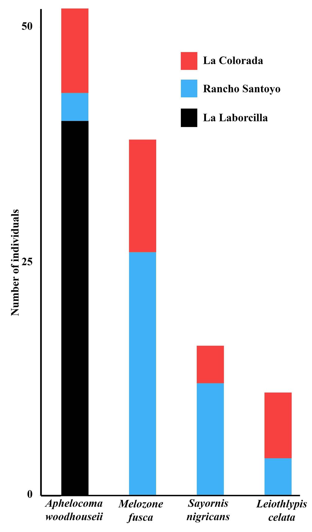
Figure 5. Total abundance of species that had location as part of the best model exploring the influence of locality and survey month, during the 2019-2020 non-breeding season in each of 3 xeroriparian systems in the Llanos de Ojuelos, southern Mexican Altiplano.
La Laborcilla had a total bird count of 213 individuals (162 of 13 resident/breeding species, 48 of 8 migrant species, and 3 of 2 unidentified species), Rancho Santoyo had 353 (197/22, 149/11, and 7/3), and La Colorada, 366 (228/27, 128/16, and 10/3). Most individuals counted were of resident species or of 1 Summer (breeding) resident species (Myiarchus cinerascens),while migrants were a smaller component of the community (Fig. 2). For species richness, the best model did not include locality nor month. The best model explaining overall bird abundance included month (Supplementary material 3), but not locality. Abundance increased from Autumn (September) to Spring (March) with some differences between guilds. Insectivore migrants increased in number into the Winter and then decreased, while granivore migrants began to arrive in December and increased until March (Fig. 2). In all these cases the month of survey was part of the best model, as it was of 11 bird species (Figs. 3, 4; Supplementary material 3). Locality was part of the best model explaining abundance in 4 cases out of 27, all of them individual species (Fig. 5; Supplementary material 3). Aphelocoma woodhouseii and Leiothlypis celata were the only 2 species whose best model included both locality and moth, while the best models for the other species did not include either variable (Supplementary material 3).

Figure 6. Total abundance of birds in different trophic guilds in 3 xeroriparian systems and 3 sections within each, during the 2019-2020 non-breeding season in the Llanos de Ojuelos, southern Mexican Altiplano. Numbers on the circles indicate richness and total abundance, while numbers on the side of the dendrograph indicate similarity between xeroriparian systems, Bird assemblages in Rancho Santoyo and La Colorada were more similar between them than to La Laborcilla (Fig. 6). In PCA graphs, the 3 sections at La Laborcilla grouped closer to each other than those of the other systems. The sections within each system grouped discreetly when binary data was used (Fig. 7 top), but groups overlapped when based on abundance (Fig. 7 bottom). The 3 systems studied differed in the resident/breeding vs. migrant composition of the communities, and sections within systems were also different (Fig. 6). Whereas Rancho Santoyo had a higher proportion of insectivore migrants than the other locations, La Colorada had a higher count of granivore migrants, and La Laborcilla had proportionally more individuals of resident species (Myiarchus cinerascens did not occur in La Laborcilla). In neither case did such patterns occur in the 3 sections of the corresponding system, but only in 2 of Rancho Santoyo’s sections and in 1 and partially in another at La Colorada.

Figure 7. Principal Component arrangement of 3 study sections in each of 3 xeroriparian systems based on their bird composition during the 2019-2020 non-breeding season in the Llanos de Ojuelos, southern Mexican Altiplano. The upper figure is based on binary data (presence/absence of species), and the lower figure, on bird abundance. Ellipses were drawn around the 3 sections of each system by hand. The legends “Up”, “Md”, and “Lw” indicate the upper, middle and lower sections of each system.
The attributes of the plant communities were different between xeroriparian systems (Table 4). La Laborcilla had significantly less ground covered by herbs, whereas Rancho Santoyo and La Colorada were not different in this aspect. La Colorada had significantly denser vegetation from 0 to 75 cm above the ground than the 2 other systems, but visual obstruction at 75-100 cm was not different between the 3 systems. The tallest shrubs and highest trees were significantly taller in Rancho Santoyo than in La Laborcilla, whereas La Colorada was not different from either, and average height both shrubs and trees was significantly greater at Rancho Santoyo than at La Laborcilla, with La Colorada being in between and statistically different from either. Canopy cover was not different between systems. Study sections were all peculiar within the systems, but only in some cases were sections significantly different (Supplementary material 4). Despite slight differences, visual obstruction at the 4 heights assessed was highest in September and October, and then decreased towards their lowest values in March (Fig. 8).
At least 1 habitat attribute was part of the best bird model in all but 3 cases (Tables 5-7), the 3 of them resident species: Zenaida asiatica, Thryomanes bewickii, and Phainopepla nitens. In all cases in which canopy cover was part of the best model, it had a negative effect on bird richness or abundance, while herb density and visual obstruction at 25-75 cm had a negative effect in most of the best models that included them (Tables 5-7). In contrast, visual obstruction at 75-100 cm and mean/maximum height of shrubs/trees had a positive effect.
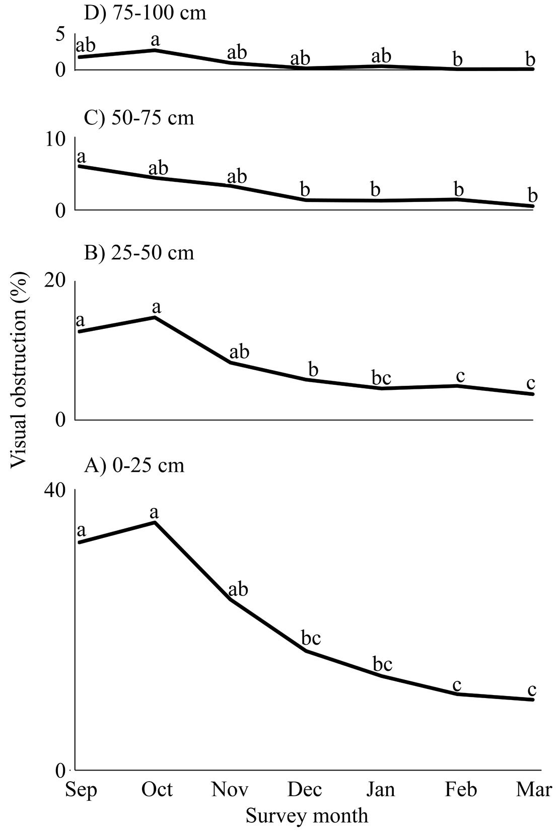
Figure 8. Mean visual obstruction in 4 25-cm vertical layers, between 0 and 100 cm above the ground across 3 sections in each of 3 xeroriparian systems studied during the 2019-2020 non-breeding season in the Llanos de Ojuelos, southern Mexican Altiplano. To reflect the spatial arrangement of the information, the panels are arranged bottom to top. The height stratum to which each graph corresponds is indicated on the graph. Points on each graph with the same letter are not statistically different (p < 0.05).
Discussion
The lack of studies about the role of ephemeral and intermittent xeroriparian systems as key habitats for biodiversity conservation and potential provision of ecological services severely impairs the capability of designing and implementing timely and informed conservation actions. In this study we generated a basic understanding about the composition of bird assemblages in 3 Mexican xeroriparian systems and the habitat attributes that influence them. Our study is particularly pertinent as the results of only 3 other research projects on birds in Mexican xeroriparian systems have been published (Arizmendi et al., 2008; Hinojosa-Huerta et al., 2013; Pérez-Amezola et al., 2020), none of them including ephemeral systems.
The 48 terrestrial species that we recorded represent 20% of all potential terrestrial native birds of the area, excluding swifts (family Apodidae) (based on Howell and Webb [1995]). This is relevant considering that xeroriparian systems, in general, occupy around 5% of the total land surface in western North America (Krueper, 2000), and that those we studied covered approximately 0.1% of the area in which they are located (by delineating them in Google Earth and measuring their area as well as that of the displayed image). According to Partners of Flight (2023) Campylorhynchus brunneicapillus, Spizella atrogularis, Selasphorus rufus/sasin, and Cardellina pusilla have conservation problems, while Accipiter striatus and A. cooperii are protected by Mexican law (Semarnat, 2010). The importance of xeroriparian systems in the region studied is enhanced by the fact that some otherwise woodland bird species largely depend on them, and we have not documented them in any other xeric habitats of the region (Mellink et al., 2016, 2017; Riojas-López & Mellink, 2019; Riojas-López et al., 2019).
Table 4
Vegetation attributes of 3 xeroriparian systems in the Llanos de Ojuelos, southern part of the Mexican Plateau, 2019-2020. Values are estimate ± standard error, except on maximum and minimum heights. Values of any variable with different literal were significantly different (p ≤ 0.05) according to an ANOVA + Tukey post hoc tests. Superscript “ns” indicates that the means were not significantly different.
| Site/section | Herb | Visual obstruction (%) | Hight of shrubs (m) | Height of trees (m) | Canopy | |||||||
| density (1-4) | 0-25 cm | 25-50 cm | 50-75 cm | 75-100 cm | Max | Min | Mean | Max | Min | Mean | cover (%) | |
| La Laborcilla | 1.53 ± 0.38b | 12.00 ± 4.27b | 4.22 ± 2.58b | 0.89 ± 1.06b | 0.40 ± 0.55ns | 2.63 ± 0.32b | 0.23 ± 0.10ns | 0.63 ± 0.01c | 8.37 ± 0.27b | 0.73 ± 0.26ns | 3.58 ± 0.26c | 40.40 ± 8.82ns |
| Rancho Santoyo | 2.52 ± 0.88a | 13.60 ± 16.7b | 3.03 ± 4.75b | 0.85 ± 2.38b | 0.83 ± 2.27ns | 3.55 ± 0.49a | 0.31 ± 0.08ns | 1.41 ± 0.31a | 14.65 ± 3.04a | 1.20 ± 0.44ns | 4.79 ± 0.89a | 39.50 ± 16.83ns |
| La Colorada | 2.70 ± 0.95a | 35.98 ± 17.06a | 16.04 ± 10.83a | 6.40 ± 6.32a | 1.59 ± 2.48ns | 3.14 ±0.76ab | 0.22 ± 0.06ns | 1.21 ± 0.44b | 10.36 ± 3.55ab | 0.87 ± 0.19ns | 4.54 ± 0.54b | 45.48 ±29.86ns |
These species can be considered locally xeroriparian-dependent. They are Accipiter striatus, A. cooperii, Empidonax difficilis occidentalis, Pitangus sulphuratus, Empidonax wrightii, Corthylio calendula, Turdus migratorius, Setophaga coronata, Setophaga townsendi, Piranga ludoviciana, Bubo virginianus, Sphyrapicus varius, and Cardinalis cardinalis. This was also the case of Pipilo maculatus and P. chlorurus, otherwise species of thick shrublands. The system with more xeroriparian-dependent species was La Colorada (9 species) followed by Santoyo (7) and La Laborcilla (6). However, Santoyo had more riparian-dependent individuals (139) than La Colorada (78) and La Laborcilla (45), Setophaga coronata and Corthylio calendula being the most abundant species (Supplementary material 2).
Table 5
Sign of the effects of habitat features on the bird community variables in 3 study sections in each of 3 xeroriparian systems studied during the 2019-2020 non-breeding season in the Llanos de Ojuelos, southern Mexican Altiplano. The only data indicated are that of variables included in the best or more parsimonious model under an information-theoretic approach. Blank cells are of variables not included in such models. Min. indicates minimum, and Max., maximum. Variables with correlation coefficients > 0.85 were merged before the analysis. The intercept is not shown. Actual data is presented in Supplementary material 5.
| Bird community variable | Herb | Visual obstruction (%) | Shrub Min. | Tree Min. | Shrub-tree | Canopy | ||
| Density (1-4) | 0-0.25 cm | 25-75 cm | 75-100 cm | Height (m) | Height (m) | Min./Max. (m) | Cover (%) | |
| Richness | + | – | ||||||
| Abundance | ||||||||
| Overall | – | – | + | – | ||||
| All resident species | – | – | – | |||||
| All migrants | – | + | + | |||||
| Migrant insectivorous birds | – | + | – | |||||
| Migrant granivorous birds | – | + | – |
Table 6
Sign of the effects of habitat features on the abundance of resident species of birds in 3 study sections in each of 3 xeroriparian systems studied during the 2019-2020 non-breeding season in the Llanos de Ojuelos, southern Mexican Altiplano. The only data indicated are that of variables included in the best or more parsimonious model, under an information-theoretic approach. Blank cells are of variables not included in such models. Min. indicates minimum, and Max., maximum. Variables with correlation coefficients > 0.85 were merged before the analysis. The intercept is not shown. Actual data is presented in Supplementary material 5.
| Bird response variable | Herb | Visual obstruction (%) | Shrub Min. | Tree Min. | Shrub-tree | Canopy | ||
| Density (1-4) | 0-0.25 cm | 25-75 cm | 75-100 cm | Height (m) | Height (m) | Min./Max. (m) | Cover (%) | |
| Zenaida asiatica | ||||||||
| Melanerpes aurifrons | – | |||||||
| Sayornis nigricans | + | |||||||
| Aphelocoma woodhouseii | – | – | ||||||
| Psaltriparus minimus | – | + | – | – | ||||
| Phainopepla nitens | ||||||||
| Thryomanes bewickii | ||||||||
| Mimus polyglottos | + | |||||||
| Spinus psaltria | + | + | + | – | ||||
| Spizella passerina | – | – | – | |||||
| Melozone fusca | + | |||||||
| Pipilo maculatus | – | + | – |
Table 7
Sign of the effects of habitat features on the abundance of migratory birds in 3 study sections in each of 3 xeroriparian systems studied during the 2019-2020 non-breeding season in the Llanos de Ojuelos, southern Mexican Altiplano. The only data indicated are that of variables included in the best or more parsimonious model, under an information-theoretic approach. Blank cells are of variables not included in such models. Min. indicates minimum, and Max., maximum. Variables with correlation coefficients > 0.85 were merged before the analysis. The intercept is not shown. Actual data is presented in Supplementary material 5.
| Bird response variable | Herb | Visual obstruction (%) | Shrub Min. | Tree Min. | Shrub-tree | Canopy | ||
| Density (1-4) | 0-0.25 cm | 25-75 cm | 75-100 cm | Height (m) | Height (m) | Min./Max. (m) | Cover (%) | |
| Empidonax wrightii | + | |||||||
| Corthylio calendula | – | + | ||||||
| Troglodytes aedon | + | |||||||
| Turdus migratorius | – | – | + | – | ||||
| Melospiza lincolnii | – | – | + | – | ||||
| Spizella pallida | – | + | – | + | – | |||
| Leiothlypis celata | + | |||||||
| Setophaga coronata | – | |||||||
| Cardellina pusilla | + |
Resident species increased their abundance from December through March (Figs. 2, 3), a pattern that could have been driven by 3 processes, not necessarily mutually exclusive: 1) resident species that might breed in xeroriparian habitats disperse to feed in other habitats in the region after nesting, might have begun to congregate for the upcoming breeding season, which would make the different habitats complementary (Dunning et al., 1992); 2) species like the P. maculatus might become more detectable as breeding-associated territoriality and courting behaviors develop; 3) migrating individuals of northern populations of species that locally remain resident might pass through the region in the Spring (perhaps S. passerina; Fig. 4).
The increase in abundance of the resident species as the season progressed was combined with the addition of migratory species in their northbound Winter-Spring migration. The pattern observed in our study is similar to that in the lower Colorado River in southwestern Arizona, where more birds migrate during the Spring than during the Autumn and suggests that some species migrate via different routes and/or use different habitats during the latter (Carlisle et al., 2009). According to our data, the region is part of the Spring migration route, but not, or less so, of the Autumn route.
Birds assemble differently in response to habitat characteristics (Wiens & Rotenberry, 1981), although bird-habitat relationships are complex (Strong & Bock, 1990). In our study, habitat characteristics were part of the best model in 78% of the cases (Tables 5-7). Three habitat variables more consistently affected bird assemblages and species. The first was that the averaged minimum and maximum height of shrubs and trees influenced birds positively, which conforms with general known principles in bird ecology (Brand et al., 2008; MacArthur & MacArthur, 1961; Merrit & Bateman, 2012; Rockwell & Stephen, 2018), and with findings in other xeroriparian systems (Brand et al., 2008). The second was that closed canopies had a negative effect. Closed canopies have been found to influence birds negatively by reducing light at ground level resulting in a less developed herb and shrub community (Beedy, 1981). The third case was that herb vertical density at 25-75 cm had also a negative effect. But this is a spurious outcome that resulted from the dense herb layer at the beginning of the study (Fig. 8), when bird abundance variables were lower, while the circannual process of herbs drying and decaying in the late Autumn and early Winter causes low herb cover coinciding with the increase in bird abundance (Figs. 2, 3).
The bird assemblages of the xeroriparian systems studied not only were different from each other, but also varied internally, between sections (Figs. 6, 7). The arrangement of the 9 sections according to their species presence/absence in axis 1, explaining 33% of the variance, follows a clear gradient (Fig. 7 top). On the left side are sections with steep, narrow, and rocky ravines with large boulders, dominated by oaks and junipers that form a close canopy with little understory herbaceous vegetation. On the right, wide and open pebbled washes, dominated by a more heterogeneous tree community composed of peppertrees, arborescent nopales, and huisaches, with a well-developed herbaceous layer. The bird communities responded to this gradient with increasing richness and abundance from left to right.
In the same graph, axis 2 follows a gradient from a well-developed shrub community and abundant litter and wetter soil to no or scarce shrubs with a dense herbaceous layer and drier ground. This gradient apparently drives the food resources available to birds, as suggested by the preponderant bird guilds in the different sections (Fig. 6): insects in its lower end to seeds in the upper end. Overall, La Colorada with the most heterogeneous sections, vegetation-wise, had also the richest bird assemblage, while La Laborcilla, with the most homogenous sections, had the poorest one, with Rancho Santoyo intermediate in both attributes (Table 4; Fig. 6; Supplementary material 5). Using bird abundance instead of binary information rearranged the PCA graph layout (Fig. 7 lower) because of the effect of species that were widespread and abundant, but without losing a resemblance to the species presence/absence PCA.
Vertical structure is important for birds, but floristic composition can also influence their diversity (Fleishman et al., 2003; Rotenberry, 1985). For example, oaks are of little attraction to most birds (Powell & Steidl, 2015), and their dominance at La Laborcilla and the upper section of La Colorada coincided with the lower richness and abundance of their bird assemblages (Fig. 6; Supplementary material 2). Rancho Santoyo supported more xeroriparian-dependent individuals, mostly of Setophaga coronata and Corthylio calendula, both small insectivorous birds. The middle and upper sections where these 2 species thrived had large cottonwoods (Populus fremontii) and willows (Salix bonplandiana). In contrast, in the middle section of La Colorada, which also had tall trees but were peppertrees and arborescent nopales, these 2 bird species were much less abundant.
Each of the systems studied had a distinct signature given by one species or dominant bird guild(s), although such signature was largely due to the assemblages in the individual sections (Fig. 6). The signature species at Laborcilla was Aphelocoma woodhouseii, whose primary habitat includes oak and juniper forests, where it typically feeds on juniper berries in the Autumn and Winter (Fig. 5; Cornell Lab of Ornithology, 2019). Although the upper Colorada section grouped with La Laborcilla, with which it shared oaks, lacked junipers and was not used by Aphelocoma woodhouseii. Their close PCA grouping rather resulted from their shared poor bird assemblages. Rancho Santoyo can be identified with migrant insectivorous birds and La Colorada with migrant granivorous birds, in concordance with the explanation on the PCA arrangement provided above.
The lower proportion and abundance of migratory insectivorous birds and absence of granivorous birds at La Laborcilla might have been caused by its less developed understory vegetation and enclosed canyon conditions. In contrast, Rancho Santoyo´s upper and middle section provided the best habitat for insectivore migrants. This system was exuberant in herb and shrub foliage, likely as a result of the longer presence of ground humidity, but had also plenty of sunny spots; and the system bordered open rangeland, providing lengthy, sharp borders, especially in its upper and middle sections. Granivore migrants were a small component of the communities we documented, and they were present almost exclusively in La Colorada´s middle section. This site had an open canopy and combined taller shrubs with denser and taller herbs than in the other sections of the same and the 2 other systems, providing higher habitat heterogeneity and, likely, more seeds. A more developed herb-shrub stratum at 0-75 cm at La Colorada than at other sites provided good escape cover adjacent to open patches that provided seeds (Table 4; Supplementary material 4).
As our data exhibit, habitats associated with non-perennial xeroriparian streams are far from uniform, not only between systems but also within them. At a landscape level they are clearly keystone structures, at least for the birds but surely for other groups as well, both collectively and individually. The 3 systems studied by us cover about 55 ha, roughly 0.1% of the area in which they occur. However, they supported 20% of the potential species of terrestrial birds of the region, including 15 that we have recorded only in such riparian habitat. Our data exhibit that in addition to their importance for resident species, some ephemeral and intermittent xeroriparian habitat in the southern part of the Mexican Altiplano are important for northbound Spring migrating birds.
Our study is a first approximation to the ecological role of xeroriparian systems in the region. However, many issues, like their importance as nesting habitat, provision of food, climatic protection, interaction with adjacent and farther away habitats, among others, remain to be studied. Nevertheless, if these xeroriparian habitats disappear, regional biodiversity would be impacted. Not only 1 or a few, but many or all xeroriparian systems, and their different sections in the region studied by us should be targeted for conservation management. Xeroriparian systems have long been considered important elements of the landscape and their conservation needs recognized. However, such consideration, and the actions derived from it, usually focus on perennial streams with their lush arboreal communities. This focus is biased and excludes an important part of xeroriparian habitat: that created by ephemeral and intermittent streams. Despite their low consideration in research and in conservation agendas, as our study and a few others have demonstrated, ephemeral and intermittent xeroriparian habitat can play a crucial role in arid and semiarid lands (Johnson & Haight, 1985; Levick et al., 2008; Sánchez-Montoya et al., 2017; Szaro & Jakle, 1985). Despite covering less than 0.1% of the region´s area, in our study they supported 20% of all terrestrial species that we documented in the region (Mellink et al., 2016, 2017; Riojas-López & Mellink, 2019; Riojas-López et al., 2019), while those that we documented only in xeroriparian systems account for 9% of all species documented. A scenario of ecological importance of non-perennial xeroriparian systems and research and management neglect are likely to occur in many other arid and semiarid regions of the world. Hence, it might be time to join forces and impulse a global agenda for their conservation, which is now especially pertinent in view of the ongoing climate change in which drier and hotter regimes are predicted.
Acknowledgements
Jaime Luévano Esparza, David H. Almanzor, Santiago Cortés, and Marco A. Carrasco assisted during field work. Access and research permission were granted kindly by owners Family Santoyo (Rancho Santoyo) and Enrique Campos (La Laborcilla), and ranch manager Melquíades Contreras (La Colorada). Ezequiel Martínez and Margarita Chávez provided logistic support. Two anonymous reviewers provided extensive and valuable comments. Our greatest appreciation to all of them. Financial support was provided by the Centro de Investigación Científica y de Educación Superior de Ensenada (CICESE), the Universidad de Guadalajara, and the first two authors´ personal funds. The Consejo Nacional de Humanidades, Ciencias y Tecnologías supported MM-O through a M.Sc. scholarship.
References
Arizmendi, M. D., Dávila, P., Estrada, A., Figueroa, E., Márquez-Valdelamar, L., Lira, R. et al. (2008). Riparian mesquite bushes are important for bird conservation in tropical arid Mexico. Journal of Arid Environments, 72,1146–1163. https://doi.org/10.1016/j.jaridenv.2007.12.017
Beedy, E. C. (1981). Bird communities and forest structure in the Sierra Nevada of California. Condor, 83,97–105. https://doi.org/10.2307/1367415
Brand, L. A., White, G. C., & Noon, B. R. (2008). Factors influencing species richness and community composition of breeding birds in a desert riparian corridor. Condor, 110,199–210. https://doi.org/10.1525/cond.2008.8421
Burnham, K. P., & Anderson, D. R. (2002). Model selection and multimodel inference: A practical information-theoretic approach. 2nd Ed. New York: Springer-Verlag.
Carlisle, J. D., Skagen, S. K., Kus, B. E., Van Riper III, C., Paxtons, K. L., & Kelly, J. F. (2009). Landbird migration in the American West: recent progress and future research directions. Condor, 111,211–225. https://doi.org/10.1525/cond.2009.080096
Challenger, A. (1998). Utilización y conservación de los ecosistemas terrestres de México. México D.F.: Comisión Nacional para el Conocimiento y Uso de la Biodiversidad, Instituto de Biología (UNAM), and Agrupación Sierra Madre.
Chesser, R. T., Billerman, S. M., Burns, K. J., Cicero, C., J. L. Dunn, J. L., Hernández-Baños, B. E. et al. (2023). Check-list of North American Birds (online). American Ornithological Society. Retrieved on March 14th, 2024 from: https://checklist.americanornithology.org/taxa/
Conabio (Comisión Nacional para el Conocimiento y Uso de la Biodiversidad). (1998). La diversidad biológica de México: estudio de país. México D.F.: Comisión Nacional para el Conocimiento y Uso de la Biodiversidad.
Conabio (Comisión Nacional para el Conocimiento y Uso de la Biodiversidad). (2008). Capital natural de México, vol. I: Conocimiento actual de la biodiversidad. México D.F.: Comisión Nacional para el Conocimiento y Uso de la Biodiversidad.
Cornell Lab of Ornithology (2019). Woodhouse´s Scrub-Jay. Retrieved on June 7th, 2023 from: https://www.allaboutbirds.org/guide/Woodhouses_Scrub-Jay/lifehistory#
Datry, T., Bonada, N., & Boulton, A. J. (2017). Conclusions: recent advances and future prospects in the ecology and management of intermittent rivers and ephemeral streams. In T. Datry, N. Bonada, & A. J. Boulton (Eds.), Intermittent rivers and ephemeral streams: ecology and management (pp. 563–584). San Diego, CA: Academic Press.
Dunning, J. B., Danielson, B. J., & Pulliam, H. R. (1992). Ecological processes that affect populations in complex landscapes. Oikos, 65,169–175. https://doi.org/10.2307/3544901
Fleishman, E., McDonal, N., Nally, R. M., Murphy, D. D., Walters, J., & Floyd, T. (2003). Effects of floristics, physiognomy and non-native vegetation on riparian bird communities in a Mojave Desert watershed. Journal of Animal Ecology, 72, 484–490. https://doi.org/10.1046/j.1365-2656.2003.00718.x
Harker, M., García R., L. A., & Riojas-López, M. E. (2008). Composición florística de cuatro hábitats en el rancho Las Papas de Arriba, municipio de Ojuelos de Jalisco, Jalisco, México. Acta Botanica Mexicana, 85,1–29.
Hays, R. L., Summers, C., & Seitz, W. L. (1981). Estimating wildlife habitat variables. Washington DC: U.S. Fish and Wildlife Service.
Hinojosa-Huerta, O., Soto-Montoya, E., Gómez-Sapiens, M., Calvo-Fonseca, A., Guzmán-Olachea, R., Butrón-Méndez, J. et al. (2013). The birds of the Ciénega de Santa Clara, a wetland of international importance within the Colorado River delta. Ecological Engineering, 59,61–73. https://doi.org/10.1016/j.ecoleng.2013.03.005
Johnson, R. R., & Haight, L. T. (1985). Avian use of xeroriparian ecosystems in the North American warm deserts. In R. R. Johnson, C. D. Ziebell, D. R. Patton, P. F. Ffolliott, P. F., & R. H. Hamre (Tech. Coords.), Riparian ecosystems and their management: reconciling conflicting uses (pp. 156–160). General Technical Report RM-GTR-120. Fort Collins, CO: U.S. Department of Agriculture, Forest Service, Rocky Mountain Forest and Range Experiment Station.
Kirkpatrick, C., Conway, C., & LaRoche, D. (2009). Surface water depletion and riparian birds. Tucson, Arizona: Arizona Cooperative Fish and Wildlife Research Unit.
Knopf, F. L. (1985). Significance of riparian vegetation to breeding birds across an altitudinal cline. In R. R. Johnson, C. D. Ziebell, D. R. Patton, P. F. Ffolliott, & R. H. Hamre (Tech. Coords.), Riparian ecosystems and their management: reconciling conflicting uses (pp. 105–111). General Technical Report RM-GTR-120. Fort Collins, CO: U.S. Department of Agriculture, Forest Service, Rocky Mountain Forest and Range Experiment Station.
Knopf, F. L., Johnson, R. R., Rich, T., Samson, F. B., & Szaro, R. C., 1988. Conservation of riparian ecosystems in the United States. Wilson Bulletin, 100,272–284. http://www.jstor.org/stable/4162566
Krueper, D. J. (1993). Effects of land use practices on western riparian ecosystems. In D. M. Finch, & P. W. Stangel (Eds.), Status and management of neotropical migratory birds (pp. 321–330). General Technical Report RM-229. Fort Collins, CO: U.S. Department of Agriculture, Forest Service, Rocky Mountain Forest and Range Experiment Station.
Krueper, D. J. (1996). Effects of livestock management on southwestern riparian ecosystems. In D. W. Shaw, & D. M. Finch (Tec. Coords.), Desired future conditions for Southwestern riparian ecosystems: bringing interests and concerns together (pp. 281–301). General Technical Report RM-GTR-272. Fort Collins, CO: U.S. Department of Agriculture, Forest Service, Rocky Mountain Forest and Range Experiment Station.
Krueper, D. J. (2000). Conservation priorities in naturally fragmented and human-altered riparian habitats of the arid West. In R. Bonney, D. N. Pachley, R. J. Cooper, & L. Nioes (Eds.), Strategies for bird conservation: the partners in flight planning process (pp. 88–90). USDA Forest Service Proceedings RMRS-P-16. Ogden, Utah, U.S.A.: Rocky Mountain Research Station.
Levick, L., Fonseca, J, Goodrich, D., Hernández, M., Semmens, D., Stromberg, J. et al. (2008). The ecological and hydrological significance of ephemeral and intermittent streams in the arid and semi-arid American southwest. Washington D.C.: Office of Research and Development, U.S. Environmental Protection Agency.
MacArthur R. H., & MacArthur, J. W. (1961). On bird species diversity. Ecology, 423,594–598. https://doi.org/10.2307/1932254
McDonough, O. T., Hosen, J. D., & Palmer, M. A. (2011). Temporary streams: the hydrology, geography, and ecology of non-perennially flowing waters. In H. S. Elliot, & L. E. Martin (Eds.), River ecosystems: dynamics, management and conservation (pp. 259–289). Hauppauge, N.Y.: Nova Science.
Mellink, E., & Riojas-López, M. E. (2020). Livestock and grassland interrelationship along five centuries of ranching the semiarid grasslands on the southern highlands of the Mexican Altiplano. Elementa Science of the Anthropocene, 8, 20. https://doi.org/10.1525/elementa.416
Mellink, E., Riojas-López, M. E., & Giraudoux, P. (2016). A neglected opportunity for bird conservation: the value of a perennial, semiarid agroecosystem in the Llanos de Ojuelos, central Mexico. Journal of Arid Environments, 124,1–9. https://doi.org/10.1016/j.jaridenv.2015.07.005
Mellink E., Riojas-López, M. E., & Cárdenas-García, M. (2017). Biodiversity conservation in an anthropized landscape: Trees, not patch size drive bird community composition in a low-input agroecosystem. Plos One, 12, e0179438. https://doi.org/10.1371/journal.pone.0179438
Merritt, D. M., & Bateman, H. L. (2012). Linking stream flow and groundwater to avian habitat in a desert riparian system. Ecological Applications, 22, 1973–1988. https://doi.org/10.1890/12-0303.1
Neate-Clegg, M. H. C., Horns, J. J., Buchert, M., Pope, T. L., Norvell, R., Parrish, J. R. et al. (2021). The effects of climate change and fluctuations on the riparian bird communities of the arid Intermountain West. Animal Conservation, 25,325–341. https://doi.org/10.1111/acv.12755
Nieto-Samaniego, Á. F., Alaniz-Ávarez, S. A., & Camprubí, A. (2005). La Mesa Central de México: estratigrafía, estructura y evolución tectónica cenozoica. Boletín de la Sociedad Geológica Mexicana, 57, 285–318. https://doi.org/10.18268/bsgm2005v57n3a3
Partners in Flight Databases. (2023). Retrieved on July 13th,
2023 from: https://pif.birdconservancy.org/avian-conserva
tion-assessment-database-scores/
Patten, D. T., Carothers, S. W., Johnson, R. R., & Hamre, R. H. (2018). Development of the science of riparian ecology in the semi-arid western United States. In R. R. Johnson, S. W. Carothers, D. M. Finch, K. J. Kingsley, & J. T. Stanley (Tech. Eds.), Riparian research and management: past, present, future, Volume 1 (pp. 1–16). General Technical Report RM-GTR-373. Fort Collins, CO: U.S. Department of Agriculture, Forest Service, Rocky Mountain Forest and Range Experiment Station.
Pérez-Amezola, M. C., Gatica-Colima, A. B. M. Cuevas-Ortalejo, D. M., Martínez-Calderas, J. M., & Vital-García, C. (2020). Riparian biota of the Protected Area of Flora and Fauna Santa Elena canyon, Mexico. Revista Bio Ciencias, 7, e798. https://doi.org/10.15741/revbio.07.e798
Powell, B. F., & Steidl, R. J. (2015). Influence of vegetation on montane riparian bird communities in the sky islands of Arizona, USA. Southwestern Naturalist 60,65–71. https://doi.org/10.1894/MCG-09.1
Riojas-López, M. E., & Mellink, E. (2019). Registros relevantes de aves en el sur del Altiplano Mexicano. Huitzil, 20, e-513. https://doi.org/10.28947/hrmo.2019.20.2.457
Riojas-López, M. E., Mellink, E., & Almanzor-Rojas, D.H. (2019). Estado del conocimiento de los carnívoros nativos (Mammalia) en un paisaje antropizado del Altiplano Mexi-
cano: el caso de Los Llanos de Ojuelos. Revista Mexicana de Biodiversidad, 90,e902669. https://doi.org/10.22201/ib.
20078706e.2019.90.2669
Riparian Habitat Joint Venture (2004). The riparian bird conser-
vation plan: a strategy for reversing the decline of riparian associated birds in California. Ver. 2.0. Retrieved on September
28th, 2021 from: https://web.archive.org/web/2018072200
1457id_/http://www.prbo.org/calpif/pdfs/riparian_v-2.pdf
Rockwell, S. M., & Stephens, J. L. (2018). Habitat selection of riparian birds at restoration sites along the Trinity River, California. Restoration Ecology, 26,767–777. https://doi.org/10.1111/rec.12624
Rosenberg, K. V, Dokter, A. M., Blancher, P. J., Sauer, J. R., Smith, A. C., Smith, P. A. et al. (2019). Decline of the North American avifauna. Science, 366,120–124. https://doi.org/10.1126/science.aaw1313
Rosgen, D. A. (1994). A classification of natural rivers. Catena, 22,169–199. https://doi.org/10.1016/0341-8162(94)90001-9
Rotenberry, J. T. (1985). The role of habitat in avian community composition: physiognomy or floristics? Oecologia, 67,213– 217. https://doi.org/10.1007/BF00384286
Sánchez-Montoya, M. M., Moleón, M., Sánchez-Zapata, J.A., & Escoriza, D. (2017). The biota of intermittent and ephemeral rivers: amphibians, reptiles, birds, and mammals. In T. Datry, N. Bonada, & A. J. Boulton (Eds.), Intermittent rivers and ephemeral streams: ecology and management (pp. 299–322). San Diego, CA: Academic Press.
Şekercioǧlu, C. H., Loarie, S. R., Oviedo-Brenes, F., Mendenhall, C. D., Daily, G. C., & Ehrlich, P. R. (2015). Tropical countryside riparian corridors provide critical habitat and connectivity for seed-dispersing forest birds in a fragmented landscape. Journal of Ornithology, 156,343–353. https://doi.org/10.1007/s10336-015-1299-x
Semarnat (Secretaría del Medio Ambiente y Recursos Naturales). (2010). Norma Oficial Mexicana NOM-059-SEMARNAT-2010, Protección ambiental – Especies nativas de México de flora y fauna silvestres – Categorías de riesgo y especificaciones para su inclusión, exclusión o cambio – Lista de especies en riesgo. Diario Oficial de la Federación. 30 de diciembre de 2010, Segunda Sección, México.
Seymour, C. L., & Simmons, R. E. (2008). Can severely fragmented patches of riparian vegetation still be important for arid-land bird diversity? Journal of Arid Environments, 72,2275–2281. https://doi.org/10.1016/j.jaridenv.2008.07.014
Skagen, S. K., Melcher, C. P., Howe, W. H., & Knopf, F. L. (1998). Comparative use of riparian corridors and oases by migrating birds in southeast Arizona. Conservation Biology, 12,896–909. https://doi.org/10.1111/j.1523-1739.1998.96384.x
Strong, T. R., & Bock, C. E. (1990). Bird species distribution patterns in riparian habitats in southeastern Arizona. Condor, 92,866–885. https://doi.org/10.2307/1368723
Szaro, R. C., & Jakle, M. D. (1985). Avian use of a desert riparian island and its adjacent scrub habitat. Condor, 87,511–519. https://doi.org/10.2307/1367948
Wiens, J. A., & Rotenberry, J. T. (1981). Habitat associations and community structure of birds in shrubsteppe environments. Ecological Monographs, 51,21–41. https://doi.org/10.2307/
2937305

Perfil de leucocitos como biomarcador hematológicoen poblaciones de la salamandra de arroyo Ambystoma ordinarium
Carolina González-Pardo a, Ireri Suazo-Ortuño a, *, Cinthya Mendoza-Almeralla b, David Tafolla-Venegas c, Yurixhi Maldonado-López a y Esperanza Meléndez-Herrera a
a Universidad Michoacana de San Nicolás de Hidalgo, Instituto de Investigaciones sobre los Recursos Naturales, Avenida San Juanito Itzícuaro s/n, Nueva Esperanza, 58330 Morelia, Michoacán, México
b Universidad Autonóma del Estado de Hidalgo, Instituto de Ciencias Básicas e Ingeniería, Centro de Investigaciones Biológicas, Laboratorio de Ecología de Poblaciones, Km 4.5 carretera Pachuca-Tulancingo, 42184 Mineral de La Reforma, Hidalgo, México
c Universidad Michoacana de San Nicolás de Hidalgo, Facultad de Biología, Edificio R, Ciudad Universitaria, 58030 Morelia, Michoacán, México
*Autor de correspondencia: ireri.suazo@umich.mx (I. Suazo-Ortuño)
Recibido: 7 agosto 2023; aceptado: 22 febrero 2024
Resumen
La evaluación del perfil de leucocitos como biomarcador hematológico en las poblaciones de anfibios es cada vez más común en estudios ecológicos en especies amenazadas o en declive. En este estudio evaluamos y comparamos el perfil de leucocitos y el índice neutrófilos/linfocitos (N/L) en frotis de sangre periférica de Ambystoma ordinarium en 3 tipos de hábitats: conservados, urbanizados y agrícolas. Consideramos al perfil leucocitario como un endpoint inmunológico, ya que nos puede proporcionar información sobre la respuesta inmunológica del organismo. De acuerdo con los resultados encontrados, en los individuos de A. ordinarium de los sitios urbanizados y agrícolas se detectaron aumentos en las proporciones de eosinófilos, basófilos y monocitos, y una disminución en las proporciones de linfocitos. Asimismo, en los individuos de los sitios urbanizados y agrícolas se detectaron aumentos en el número de neutrófilos banda, además se reporta por primera vez el hallazgo de células plasmáticas en la sangre de esta especie. En general, los perfiles de leucocitos de los individuos de A. ordinarium en los sitios urbanizados y agrícolas observados en este estudio, podrían interpretarse como respuestas fisiológicas a la perturbación ambiental.
Palabras clave: Hábitats perturbados; Respuesta inmunitaria; Índice N/L; Neutrófilos banda; Células plasmáticas; Achoque michoacano
© 2024 Universidad Nacional Autónoma de México, Instituto de Biología. Este es un artículo Open Access bajo la licencia CC BY-NC-ND
(http://creativecommons.org/licenses/by-nc-nd/4.0/).
Leukocyte profile as hematologic biomarker in populations of the mountain salamander, Ambystoma ordinarium
Abstract
Assessing the leukocyte profile as a hematological biomarker is now frequently used in ecological studies of threatened or declining species. In this study, we evaluated and compared leukocytes profile and neutrophils/lymphocytes (N/L) ratio in peripheral blood smears of the salamander Ambystoma ordinarium in 3 types of habitats: urbanized, agricultural, and conserved. We considered leukocyte profiles as an immunological endpoint, since it can provide information about the immunological response. Results indicated that A. ordinarium individuals from the urbanized and agricultural sites presented higher proportions of neutrophils, eosinophils, basophils and monocytes and a decrease in the proportions of lymphocytes. Agricultural habitats presented higher N/L ratios. Likewise, in the individuals of urbanized and agricultural sites an increase was registered in the number of neutrophils with a band nucleus, in addition, the finding of plasma cells in the blood of this species is reported for the first time. In general, leukocyte profiles of A. ordinarium individuals in urbanized and agricultural sites observed in this study suggest that these profiles can be interpreted as physiological responses to environmental disturbance.
Keywords: Disturbed habitats; Immune response; N/L ratio; Band neutrophils; Plasma cells; Achoque michoacano
Introducción
En la actualidad, una de las preocupaciones más importantes en la conservación de vida silvestre es la pérdida y disminución global de las especies de anfibios (Alvarado, 2021). Los cambios en los hábitats asociados a las actividades antropogénicas y las enfermedades infecciosas representan las principales amenazas (Wake y Vredenburg, 2008). Sin embargo, científicos en todo el mundo, consideran que no existe una sola causa potencial, sino que éstos y otros factores pueden actuar mediante sinergias contribuyendo en la disminución de sus poblaciones (Lips et al., 2005; Stuart et al., 2004).
Los anfibios, pueden ser más vulnerables a los cambios en sus hábitats en comparación con el resto de los vertebrados, por 2 razones principales: poseen una piel delgada y porosa que es permeable al agua, y son organismos ectotermos, por lo que dependen de su entorno para conservar su temperatura (Duellman y Trueb, 1994). Por estos motivos, la evaluación del estado de salud de las poblaciones de anfibios es cada vez más común en estudios ecológicos en especies amenazadas o en declive (Barriga-Vallejo et al., 2015; Das y Mahapatra, 2014; Shutler y Marcogliese, 2011). Los perfiles de leucocitos han sido evaluados con mayor frecuencia porque proporcionan información sobre el estado inmunológico y permiten detectar cambios fisiológicos y patológicos tempranos en los individuos, sobretodo, estudios recientes han comenzado a incorporarlos como biomarcadores para evaluar la salud de los individuos y de su ambiente (Barni et al., 2007; Cabagna et al., 2005; Davis et al., 2010; Salinas et al., 2015, 2019).
Los leucocitos (linfocitos, neutrófilos, eosinófilos, basófilos y monocitos) son células sanguíneas que forman parte del sistema inmunitario, desempeñando funciones cruciales en la defensa contra infecciones y enfermedades (Thrall, 2004). De esta forma, los leucocitos en sangre pueden aumentar rápidamente en una infección, por ejemplo, aumentos en las proporciones de eosinófilos se han asociado con infecciones parasitarias (Davis y Golladay, 2019; Ramírez-Hernández et al., 2019) y en evidencia reciente, se han reportado aumentos en las frecuencias de linfocitos maduros e inmaduros (Salinas et al., 2019). El perfil de leucocitos también ha sido evaluado con éxito como indicador de estrés en poblaciones en ambientes perturbados y alteraciones morfológicas como el aumento de neutrófilos sin segmentación nuclear se han relacionado con ambientes contaminados con desechos urbanos y agrícolas (Barni et al., 2007; Cabagna et al., 2005; Ramírez-Hernández et al., 2019; Romanova y Romanova, 2003).
En México, habitan 14 especies del género Ambystoma (Ramírez-Bautista et al., 2023) y se ha estudiado el perfil de leucocitos en algunas especies como biomarcador de inflamación y estrés asociado a perturbaciones antropogénicas (Barriga-Vallejo et al., 2015; Ramírez-Hernández et al., 2019). La salamandra de arroyo Ambystoma ordinarium se distribuye en el noreste de Michoacán y se encuentra catalogada como en peligro de extinción por la IUCN (2024), y como especie protegida por el gobierno de México (Semarnat, 2010). Particularmente, en varios sitios del área de distribución de esta especie existe un fuerte impacto sobre los arroyos que habita debido a presiones de urbanización, actividades agrícolas y ganaderas (Soto-Rojas, 2012). Considerando el contexto en el que se encuentra esta especie, es importante monitorear sus poblaciones, sobre todo las que están sujetas a la continua perturbación de sus hábitats. Por lo tanto, el objetivo de este estudio fue evaluar y comparar los perfiles de leucocitos como biomarcador hematológico en poblaciones de A. ordinarium de hábitats con diferentes grados de perturbación: conservados, urbanizados y agrícolas.
Materiales y métodos
Se realizaron 2 visitas, la primera en noviembre de 2020 y la segunda en marzo de 2021 a 9 sitios con arroyos habitados por A. ordinarium condiferentes grados de perturbación en Michoacán (fig. 1).Los sitios 1, 2 y 3 se encuentran en zonas conservadas en los municipios de Charo, Morelia y Zinápecuaro. En estos sitios, la vegetación está representada por bosque de pino y pino-encino y no se encuentran afectados por la urbanización, cultivos ni zonas de pastoreo.
Los sitios 4, 5 y 6 son urbanizados y se localizan en la Ciudad de Morelia, la cual tiene una extensión de 1,333 km2 y presenta más de 500,000 habitantes (Magaña-Martínez y Reyes Camacho, 2012; tabla 1, fig. 1). Cada sitio se encuentra a una distancia mínima de 3 km uno con respecto a otro, por lo que corresponden a 3 poblaciones independientes de acuerdo a la poca vagilidad de la especie reportada por Montes-Calderón et al. (2011). Se consideraron los sitios como perturbados debido a: 1) la presencia de construcciones urbanas (López- Granados et al., 2008; Magaña-Martínez y Reyes Camacho, 2012), 2) el vertimiento de aguas contaminadas con fertilizantes y pesticidas (López- Granados et al., 2008) y 3) se encuentran a menos de 1 km de avenidas principales de la ciudad de Morelia (Téllez-Ramírez, 2012).
Los sitios 7, 8 y 9 se encuentran en zonas agrícolas en los municipios de Queréndaro, Indaparapeo y Zinapécuaro (fig. 1). Estos sitios presentan arroyos permanentes con escasa vegetación ribereña y se consideran perturbados porque durante el muestreo de este estudio, estaban rodeados de cultivos de maíz y potreros, y no presentaban vegetación de bosque de pino y pino-encino.
En cada arroyo se realizó una búsqueda intensiva de los ejemplares mediante la técnica de inspección por encuentro visual (VES) (Crump y Scott, 1994). Una vez localizados, se capturaron con red de mano y se colocaron en recipientes con agua de su medio para evitar su desecación. Inmediatamente, en el sitio de colecta, se manipuló a cada ejemplar con guantes estériles y se obtuvo una gota de sangre periférica de un pequeño corte de una de las branquias, llevando a cabo el procedimiento sin sacrificar a los individuos. La gota de sangre se colocó en el extremo de un portaobjetos limpio y con ayuda de un segundo, el cual se colocó en un ángulo de 45° por delante de la gota, se lo hizo retroceder hasta tocar la gota, luego se deslizó ejerciendo una presión suave y firme hacia delante. Cada frotis sanguíneo se secó a temperatura ambiente por 3 min y se fijó con metanol. Al final del procedimiento todos los organismos se liberaron en sus respectivos arroyos de origen. El manejo de las salamandras y las muestras se realizó con el permiso de colecta científica número SGPA/DGVS/13339/19 otorgado por la Semarnat.
Los frotis sanguíneos fueron llevados al laboratorio de Parasitología de la Universidad Michoacana de San Nicolás de Hidalgo (UMSNH) y se cubrieron con el colorante no diluido de Wright, dejándose reposar durante 5 min. Posteriormente, se les agregó solución buffer de Wright gota a gota, hasta que apareció una película metálica sobre la muestra, después se dejaron reposar por 5 min. Finalmente, los frotis fueron lavados con agua destilada, hasta que el colorante se lavó y se dejaron secar.

Figura 1. Mapa de la ubicación de los sitios de estudio de A. ordinarium en algunos municipios de Michoacán. 1. 5.7 km al este de Jaripeo, 2. Agua Zarca, 3. 8.9 km al oeste de Bocaneo, 4. Puente campestre, 5. Filtros viejos, 6. Río Chiquito, 7. 14 km al sur de Queréndaro, 8. 0.75 km al sur de Ziróndaro, 9. 10.86 km al sureste del Municipio de Queréndaro.
Tabla 1
Datos de colecta de Ambystoma ordinarium. Se muestra el nombre, las coordenadas y la categoría de los sitios de colecta y el número y talla de los organismos colectados.
| Número y nombre de sitio | Coordenadas | Categoría del sitio | Individuos colectados en invierno 2020 | Individuos colectados en primavera 2021 | Longitud LHC en mm |
| 1. 5.7 km al este de Jaripeo | 19°40’28.3” N, 101°01’44.9” O | Conservado | 4 | 3 | 74 a 77 |
| 2. Agua Zarca | 19°34’28.9” N, 101°07’28.2” O | Conservado | 3 | 13 | 66 a 77 |
| 3. 8.9 km al oeste de Bocaneo | 19°50’28.6” N, 100°43’55.1” O | Conservado | 0 | 13 | 67 a 88 |
| 4. Puente campestre | 19°40’31.3” N, 101°09’27.5′′ O | Urbanizado | 3 | 3 | 79 a 98 |
| 5. Filtros Viejos | 19°40’01.0” N, 101°08’36” O | Urbanizado | 5 | 8 | 77 a 91 |
| 6. Río Chiquito | 19°36’38.2” N, 101°07’26.8” O | Urbanizado | 7 | 5 | 81 a 101 |
| 7. 14 km al sur de Queréndaro | 19°41’05.2” N, 100°52’31.2” O | Agricola | 5 | 11 | 75 a 94 |
| 8. 0.75 km al sur de Ziróndaro | 19°42’58.4” N, 100°54’59.6” O | Agricola | 9 | 8 | 67 a 118 |
| 9. 10.86 km al sureste del Municipio de Queréndaro | 19°45’25.4” N, 100°50’33.9” O | Agricola | 4 | 5 | 82 a 111 |
Cada frotis se observó al microscopio óptico con el aumento 400x y se efectuó el recuento diferencial de leucocitos en movimiento zigzag. Las células fueron contadas por una sola persona para evitar la variabilidad en las observaciones considerando las características morfológicas descritas por Thrall (2004), Hadji-Azimi et al. (1987) y Salinas et al. (2017). Siguiendo a Davis et al. (2008), en cada frotis sanguíneo se contaron 100 células, determinándose las proporciones relativas de los 5 tipos de leucocitos y el índice N/L propuesto como indicador de respuesta al estrés. Para la evaluación morfológica de los leucocitos, durante el recuento diferencial, se contaron los leucocitos con cambios en la coloración y presencia de manifestaciones morfológicas en el citoplasma; además, se evaluó la segmentación nuclear de los neutrófilos (neutrófilos banda, identificados por la falta de segmentación en el núcleo).
Para comparar las proporciones y la morfología de cada tipo de leucocito y los índices N/L de los individuos de A. ordinarium entre los sitios conservados, urbanizados y agrícolas, se utilizaron modelos lineales generalizados mixtos (GLM), con error de distribución Poisson debido a que las variables de respuesta son conteos. Los análisis estadísticos se realizaron en R versión 4.2.0 (R Core Team, 2022) y se usó el paquete ggplot2 versión 3.4.1 (Wickham et al., 2016) para la realización de figuras.
Resultados
Se recolectaron 109 individuos de Ambystoma ordinarium en los 3 sitios, 36 en conservados, 31 en urbanizados y 42 en los agrícolas (tabla 1), 40 ejemplares se obtuvieron en invierno de 2020 y 69 en primavera de 2021. El promedio de la longitud total de los ejemplares fue de 82.44 mm (mínima 66-118 máxima) y de acuerdo con las tallas reportadas por Anderson y Worthington (1971), todos los individuos recolectados fueron adultos metamórficos (tabla 1).
Los promedios en las proporciones de los 5 tipos de leucocitos y el índice N/L de los individuos de A. ordinarium para los sitios conservados, urbanizados y agrícolas se presentan en la tabla 2. Las proporciones de linfocitos mostraron diferencias significativas entre los sitios. Se detectaron disminuciones en las proporciones de estas células en individuos de los sitios urbanizados y agrícolas en comparación con los individuos de los hábitats conservados (fig. 2). No se detectaron diferencias en las proporciones de neutrófilos y los índices N/L entre los sitios (tabla 2). Por último, las proporciones de eosinófilos, basófilos y monocitos mostraron diferencias significativas entre los sitios (tabla 2). Se detectaron aumentos en las proporciones de estas células en individuos de los sitios urbanizados y agrícolas con respecto a los individuos de los sitios conservados (fig. 2).

Figura 2. Gráfica de cajas y alambres que muestra las diferencias en las proporciones de leucocitos entre los hábitats urbanizados, agrícolas y conservados. Las letras representan las diferencias de medias entre grupos de acuerdo al GLM.
Los linfocitos, fueron los leucocitos de menor tamaño, la mayoría de éstos se caracterizaron por ser células redondas con un núcleo central que ocupó la mayor parte del citoplasma basófilo (fig. 3). En los frotis sanguíneos de 2 individuos de los hábitas agrícolas se observaron células plasmáticas, caracterizadas por un núcleo excéntrico, citoplasma abundante con aumento en la basofília y abundantes inclusiones globulares y hialinas (fig. 3).
Tabla 2
Promedios relativos de los leucocitos e índices N/L (±error estándar) en individuos adultos de Ambystoma ordinarium entre hábitats conservados, urbanizados y agrícolas.
| Variable de respuesta | Hábitats conservados | Hábitats urbanizados | Hábitats agrícolas | gl | c2 | p |
| Linfocitos | 83.1 (± 0.51) | 72.8 (± 1.20) | 74.5 (± 0.93) | 2 | 27.84 | < 0.001 |
| Neutrófilos | 8.4 (± 0.69) | 8.9 (± 0.95) | 9.6 (± 0.97) | 2 | 2.84 | 0.095 |
| Eosinófilos | 3.9 (± 0.38) | 8.3 (± 1.53) | 9.0 (± 0.84) | 2 | 88.37 | < 0.001 |
| Basófilos | 2.7 (± 0.42) | 4.9 (± 0.68) | 4.5 (± 0.52) | 2 | 26.66 | < 0.001 |
| Monocitos | 1.7 (± 0.43) | 4.9 (± 1.24) | 2.2 (± 0.39) | 2 | 63.26 | < 0.001 |
| Neutrófilos banda | 1.5 (± 0.24) | 3.1 (± 0.60) | 3.8 (± 0.48) | 2 | 42.27 | <0.001 |
| Índice N/L | 0.10 (± 0.00) | 0.10 (± 0.011) | 0.13 (± 0.01) | 2 | 0.17 | 0.698 |
Los neutrófilos se caracterizaron por ser células redondas irregulares que pueden o no presentar finos gránulos en el citoplasma, su núcleo violeta puede no presentar segmentaciones (neutrófilos banda, fig. 3) ó ser segmentados de 2 a 5 lóbulos (fig. 3). En relación con la comparación de la segmentación nuclear de los neutrófilos entre los sitios, se encontraron variaciones significativas, detectándose incrementos en las proporciones de neutrófilos banda en individuos de los sitios urbanizados y agrícolas con respecto a los individuos de los sitios conservados (fig. 3).
Los eosinófilos fueron células con abundantes gránulos rosados cubriendo el citoplasma, presentan un núcleo violeta generalmente bilobulado (fig. 3) y en pocas ocasiones se observó unilobulado y trilobulado. Con respecto de la morfología de los basófilos, éstos se caracterizaron por ser células redondas u ovaladas con abundantes gránulos púrpuras en el citoplasma que, por lo general, cubren el núcleo redondo o bilobulado (fig. 3). Por último, los monocitos fueron los leucocitos de mayor tamaño, son células redondas con núcleo en forma de riñón o herradura y citoplasma abundante (fig. 3). No se observaron variaciones morfológicas en eosinófilos, basófilos y monocitos.
Discusión
Se evaluaron los perfiles de leucocitos en frotis de sangre de 109 individuos adultos de la salamandra Ambystoma ordinarium, de los cuales 37 se recolectaron en hábitats conservados, 30 en hábitats urbanizados y 42 en hábitats agrícolas. La morfología y coloración de los 5 tipos de leucocitos concuerdan con lo reportado para otras especies de anuros y caudados (Cabagna et al., 2005; Hadji-Azimi et al., 1987; Salinas et al., 2017). Los linfocitos fueron los leucocitos más abundantes, detectándose disminuciones en sus proporciones en individuos de A. ordinarium de los sitios urbanizados y agrícolas considerados como perturbados. En estudios recientes, la disminución de los linfocitos en sangre se ha documentado en especies de anfibios como respuesta a factores estresantes como infecciones y hábitats contaminados con pesticidas, debido a que el aumento en las hormonas del estrés (glucocorticoides) puede inducir la salida de estas células de la sangre a los tejidos linfoides (en anfibios, hígado y bazo) (Davis et al., 2008; Waye et al., 2019). En contraste, los neutrófilos por ser las principales células encargadas del ataque a agentes infecciosos son estimulados a proliferar para migrar a los sitios de inflamación. La disminución en las proporciones de los linfocitos se ha relacionado con el aumento en las proporciones de los neutrófilos (índice N/L) como biomarcador de estrés (Davis et al., 2010). En este estudio, no se detectaron variaciones significativas en las proporciones de neutrófilos y en los índices N/L promedio. En estudios previos en poblaciones silvestres de salamandras del género Ambystoma y otras especies de anfibios, se han reportado índices N/L promedio cercanos a 0.40 (Cabagna et al., 2005; Davis y Durso, 2009; Shutler et al., 2009). Sin embargo, a diferencia de nuestro estudio, Ramírez-Hernández et al. (2019) reportaron para esta especie un índice N/L promedio de 1.5. y 0.9 en hábitats perturbados y conservados, respectivamente. Las diferencias entre ambos resultados podrían deberse a que el tamaño de muestra utilizado por Ramírez-Hernández et al. (2019) fue pequeño en comparación con el tamaño de muestra utilizado en nuestro estudio. Además, nuestros resultados pueden indicar que otros factores no contabilizados están influyendo en las respuestas de estas células en los individuos muestreados. Un factor que aumenta el índice linfocitos y neutrófilos en anfibios es la infección por Batrachochytrium dendrobatidis (Bd; Davis et al., 2010; Savage et al., 2016). Recientemente, se reportó la presencia del hongo quitridio en las mismas poblaciones de A. ordinarium analizadas en este estudio (Mendoza-Almeralla et al., 2023). Los niveles de infección por Bd reportados fueron de entre 112 a 1,856 equivalentes zoosporas genómicas (EZG´s) en 2 sitios conservados; mientras que en los sitios perturbados, el grado de infección fue de 21 a 4,338 EZG´s, ésto sugiere que hay mayor grado de infección en lugares perturbados. Por lo que es importante saber si el número de neutrófilos y linfocitos es afectado por la infección del quitridio.

Figura 3. Leucocitos en frotis de sangre periférica de A. ordinarium. A) Linfocito, B) neutrófilo segmentado, C) neutrófilo banda, D) eosinófilo, E) basófilo, D) monocito, vista a 100X, G) célula plasmática con núcleo excéntrico y citoplasma abundante, vista a 40X.
Por otro lado, se detectaron incrementos de neutrófilos banda en individuos de los sitios perturbados con respecto a los sitios conservados. En procesos inflamatorios, los neutrófilos son impulsados a proliferar y para compensar esta demanda, la médula ósea libera en la sangre células inmaduras (neutrófilos banda) (Davis y Golladay, 2019). En anfibios existe evidencia de incrementos en las proporciones de estas células como respuesta inflamatoria contra fertilizantes y pesticidas (Mann et al., 2009; Romanova et al., 2022). Pese a que en este estudio no evaluamos la presencia de estos contaminantes químicos en el agua, en los sitios urbanizados seleccionados aquí, se han reportado descargas de aguas contaminadas con fertilizantes y pesticidas (López-Granados et al., 2008), y en los sitios agrícolas es probable que el uso de estos agroquímicos sea habitual y su dispersión fuera de estas áreas pueda llegar hasta los arroyos donde habita esta especie. Los incrementos detectados en las proporciones de eosinófilos, basófilos y monocitos en los individuos de los sitios urbanizados y agrícolas también se pueden asociar con la presencia de estos contaminantes químicos en sus hábitats. En algunos estudios en anfibios se han reportado incrementos en las proporciones de eosinófilos en sitios contaminados por pesticidas por su capacidad de reaccionar a antígenos ambientales (Attademo et al., 2014; Romanova y Romanova, 2003). Con respecto a los monocitos, el aumento de estas células podría relacionarse con el incremento de la fagocitosis de desechos tisulares, puesto que, de acuerdo con algunos autores la exposición prolongada a contaminantes químicos aumenta la necrosis tisular (Zhelev, 2007). El papel de los basófilos en las respuestas inmunitarias de los anfibios no es claro (Allender y Fry, 2008), sin embargo, al igual que en otros grupos de vertebrados parecen desempeñar un papel importante en la inflamación (Claver y Quaglia, 2009).
Los estudios realizados por varios investigadores han revelado que los anfibios son capaces de generar una respuesta inmunitaria a antígenos complejos asociados con patógenos y antígenos ambientales (Grogan et al., 2018; Savage y Zamudio, 2011; Zhelev, 2007). Los linfocitos (células T y B), ante la presencia de antígenos son responsables de activar la inmunidad mediada por células específicas de patógenos (células T citotóxicas o auxiliares) y la inmunidad humoral (células plasmáticas secretoras de anticuerpos específicos) (Grogan et al., 2018). El hallazgo de células plasmáticas en la sangre de los individuos de los sitios agrícolas podría atribuirse a la especificidad de la respuesta inmune humoral a antígenos tóxicos presentes en el ambiente. En un estudio previo, Zhelev (2007) reportó aumentos de estas células en individuos de Rana ridibunda en hábitats con contaminación industrial. El hallazgo de estas células es interesante, porque casi no hay datos en la literatura sobre su presencia y apariencia en la sangre de los anfibios. Aunque no podemos asegurar que se trate de este tipo de células, estos datos sin duda sientan las bases para desarrollar estudios bioquímicos e inmunológicos futuros.
En anfibios se ha documentado la función antipara-
sitaria de los eosinófilos en infecciones con nemátodos y tremátodos (Belden y Kiesecker, 2005; Davis y Golladay, 2019; Kiesecker, 2002; Rohr et al., 2008). Particularmente, Ramírez-Hernández et al. (2019) reportaron aumentos en las cargas parasitarias en poblaciones de A. ordinarium por 2 especies de tremátodos, Gorgoderina attenuata y Ochetosoma sp.,y 2 especies de nemátodos Cosmocercoides sp.y Hedruris siredonis en hábitats perturbados, siendo uno de estos hábitats correspondiente al sitio Río Chiquito de este estudio. Adicionalmente, Mendoza-Almeralla et al. (2023) reportaron la infección por el nemátodo del género Capillaria en el sitio Filtros viejos. Por lo tanto, los incrementos de eosinófilos detectados en los individuos de estos sitios, podrían relacionarse con la presencia de mayor prevalencia de infecciones parásitarias.
Finalmente, los perfiles de leucocitos de los individuos de A. ordinarium en este estudio proporcionan parámetros hematológicos de comparación entre distintas poblaciones. De acuerdo con nuestros resultados, la evaluación de los perfiles de leucocitos es uno de los métodos más simples y menos invasivos. Los cambios en sus valores, especialmente en las poblaciones de hábitats perturbados, pueden utilizarse con éxito en evaluaciones futuras para detectar cambios fisiológicos y patológicos tempranos en los individuos y puede ser una señal de advertencia de degradación ambiental. Sin embargo, es importante reiterar que interpretar las proporciones de los leucocitos puede ser complicado, debido a que los leucocitos pueden responder a diversos factores (Barni et al., 2007; Cabagna et al., 2005; Romanova y Romanova, 2003; Shutler y Marcogliese, 2011; Shutler et al., 2009). Por ello es necesario llevar a cabo estudios complementarios sobre enfermedades infecciosas, calidad del agua, niveles de hormonas de estrés, presencia de pesticidas o metales pesados, entre otros, que permitan relacionar y estudiar la respuesta de los leucocitos en las poblaciones de esta especie y otras especies de anfibios con los diversos factores o contextos en los que se encuentran estas especies.
Agradecimientos
Este estudio fue parte del proyecto “Descifrando el microbioma de la piel en ajolotes y las consecuencias de la interacción huésped microbioma sobre una enfermedad letal emergente” de la Secretaría de Educación Pública/Consejo Nacional de Humanidades, Ciencias y Tecnologías Ciencias de Frontera. FORDECYT-PRONACES/373914/2020. Los resultados de este estudio forman parte de la tesis de maestría del autor principal, bajo la dirección de ISO y CMA. CGP agradece el apoyo financiero del Programa Nacional de Becas de SEP/Conahcyt.
Referencias
Allender, M. C. y Fry, M. M. (2008). Amphibian hematology. Veterinary Clinics of North America: Exotic Animal Practice, 11, 463–480. https://doi.org/10.1016/j.cvex.2008.03.006
Alvarado, J. G. A. (2021). Anfibios en peligro: amenazas y estrategias efectivas de conservación. Biocenosis, 32, 3–45. https://doi.org/10.22458/rb.v32i1.3552
Anderson, J. D. y Worthington, R. D. (1971). The life history of the Mexican salamander Ambystoma ordinarium Taylor. Herpetologica, 27, 165–176.
Attademo, A. M., Peltzer, P. M., Lajmanovich, R. C., Cabagna-Zenklusen, M. C., Junges, C. M. y Basso, A. (2014). Biological endpoints, enzyme activities, and blood cell parameters in two anuran tadpole species in rice agroecosystems of mid-eastern Argentina. Environmental Monitoring and Assessment, 186, 635–649. https://doi.org/10.1007/s10661-013-3404-z
Barni, S., Boncompagni, E., Grosso, A., Bertone, V., Freitas, I., Fasola, M. et al. (2007). Evaluation of Rana snk esculenta blood cell response to chemical stressors in the environment during the larval and adult phases. Aquatic Toxicology, 81, 45–54. https://doi.org/10.1016/j.aquatox.2006.10.012
Barriga-Vallejo, C., Hernández-Gallegos, O., Von-Herbing, I. H., López-Moreno, A. E., Ruiz-Gómez, M. D. L., Granados-González, G. et al. (2015). Assessing population health of the Toluca Axolotl Ambystoma rivulare (Taylor, 1940) from México using leukocyte profiles. Herpetological Conservation and Biology, 10, 592–601.
Belden, L. K. y Kiesecker, J. M. (2005). Glucocorticosteroid hormone treatment of larval treefrogs increases infection by Alaria sp. trematode cercariae. Journal of Parasitology, 91, 686–688. https://doi.org/10.1645/GE-397R.
Cabagna, M. C., Lajmanovich, R. C., Stringhini, G., Sánchez-Hernández, J. C. y Peltzer, P. M. (2005). Hematological parameters of health status in the common toad Bufo arenarum in agroecosystems of Santa Fe Province, Argentina. Applied Herpetology, 2, 373–380. https://doi.org/10.1163/157075405774483085
Claver, J. A. y Quaglia, A. I. (2009). Comparative morphology, development, and function of blood cells in nonmammalian vertebrates. Journal of Exotic Pet Medicine, 18, 7–97. https://doi.org/10.1053/j.jepm.2009.04.006
Crump, M. L. y Scott, N. Y. (1994). Visual encounter surveys. En W. Heyer, M. A. Donnelley, R. A. Mcdiarmid, L. C. Hayek. y M. C. Foster (Eds.), Measuring and monitoring biological diversity: standard methods for amphibians (pp. 84–92). Washington D.C.: Smithsonian Institution.
Das, M. y Mahapatra, P. K. (2014). Hematology of wild caught Dubois’s tree frog Polypedates teraiensis, Dubois, 1986 (Anura: Rhacophoridae). The Scientific World Journal, 491415, 7. https://doi.org/10.1155/2014/491415
Davis, A. K. y Durso, A. M. (2009). White blood cell differentials of northern cricket frogs (Acris c. crepitans) with a compilation of published values from other amphibians. Herpetologica, 65, 260–267. https://doi.org/10.1655/08-052R1.1
Davis, A. K. y Golladay, C. (2019). A survey of leukocyte profiles of red-backed salamanders from Mountain Lake, Virginia, and associations with host parasite types. Comparative Clinical Pathology, 28, 1743–1750. https://doi.org/10.1007/s00580-019-03015-9
Davis, A. K., Maney, D. L. y Maerz, J. C. (2008). The use of leukocyte profiles to measure stress in vertebrates: a review for ecologists. Functional Ecology, 22, 760–772. https://doi.org/10.1645/GE-397R
Davis, A. K., Keel, M. K., Ferreira, A. y Maerz, J. C. (2010). Effects of chytridiomycosis on circulating white blood cell distribu-
tions of bullfrog larvae (Rana catesbeiana). Comparative Clinical Pathology, 19, 49–55. 10.1007/s00580-009-0914-8
Duellman, W. E. y L. Trueb. (1994). The biology of amphibians. Baltimore, Maryland: Johns Hopkins University Press.
Grogan, L. F., Robert, J., Berger, L., Skerratt, L. F., Scheele, B. C., Castley, J. G. et al. (2018). Review of the amphibian immune response to chytridiomycosis, and future directions. Frontiers in Immunology, 9, 2536. https://doi.org/10.3389/fimmu.2018.02536
Hadji-Azimi, I., Coosemans, V. y Canicatti, C. (1987). Atlas of Xenopus laevis laevis hematology. Developmental and Comparative Immunology, 11, 807–874.
IUCN. (2020). Ambystoma ordinarium. The IUCN Red List of Threatened Species. Recuperado el 01 junio, 2024 de: https://www.iucnredlist.org/es/species/59066/161153310
Kiesecker, J. M. (2002). Synergism between trematode infection and pesticide exposure: a link to amphibian deformities in nature? Proceedings of the National Academy of Sciences, 99, 9900–9904. https://doi.org/10.1073/pnas.152098899
Lips K. R., Burrowes, P. A., Mendelson, J. R. y Parra-Olea, G. (2005). Amphibian population declines in Latin America: a synthesis. Biotropica, 37, 222–226. https://doi.org/10.1111/j.1744-7429.2005.00029.x
López-Granados, E., Mendoza-Cantú, M., Bocco, G. y Espinosa-Bravo, M. (2008). Patrones de degradacion ambiental en la Cuenca del Lago de Cuitzeo, Michoacán. Una perspectiva espacial. Centro de Investigaciones en Ecosistemas, UNAM/Morelia, Michoacán, Instituto de Geografía, UNAM/ Dirección General de Investigación de Ordenamiento Ecológico y Conservación de los Ecosistemas, INIFAP.
Magaña-Martínez, H. M. y Reyes-Camacho, E. (2012). Parque lineal ecológico los filtros viejos en Morelia, Mich. (Tesina). Facultad Arquitectura, Universidad Michoacana de San Nicolás de Hidalgo. Morelia, Michoacán.
Mann, R. M., Hyne, R. V., Choung, C. B. y Wilson, S. P. (2009). Amphibians and agricultural chemicals: review of the risks in a complex environment. Environmental Pollution, 157, 2903–2927. https://doi.org/10.1016/j.envpol.2009.05.015
Mendoza-Almeralla, C., Tafolla-Venegas, D., González-Pardo,
C. y Suazo- Ortuño, I. (2023). Primer registro de infección por Batrachochytrium dendrobatidis y por el nemátodo del género Capillaria y la ausencia de infección por Ribeiroia ondatrae en Ambystoma ordinarium. Revista Latinoamericana de Herpetología, 6, e615-05. https://doi.org/10.22201/fc.25942158e.2023.4.615
Montes-Calderón, A. M., Alvarado-Díaz, J. y Suazo-Ortuño, I. (2011). Abundancia, actividad espacial y crecimiento de Ambystoma ordinarium Taylor 1940 (Caudata: Ambys-
tomatidae) en Michoacán, México. Revista Biológicas, 13, 50–53.
Ramírez-Bautista, A., Torres-Hernández, L. A., Cruz-Elizalde, R., Berriozabal-Islas, C., Hernández-Salinas, U., Wilson, L. D. et al. (2023). An updated list of the Mexican herpetofauna: with a summary of historical and contemporary studies. Zookeys, 1166, 287. https://doi.org/10.3897/zookeys.1166.86986
Ramírez-Hernández, G., Suazo-Ortuño, I., Alvarado-Díaz, J., Escalera-Vázquez, L. H., Maldonado-López, Y. y Tafolla-Venegas, D. (2019). Effects of habitat disturbance on parasite infection and stress of the endangered Mexican stream salamander Ambystoma ordinarium. Salamandra, 55, 160–172.
R Core Team. (2022). R: A language and environment for statistical computing. R Foundation for Statistical Computing, Vienna, Austria. Recuperado el 01 junio, 2023 de: https://www.R-project.org/
Rohr, J. R., Schotthoefer, A. M., Raffel, T. R., Carrick, H. J., Halstead, N., Hoverman, J. T. et al. (2008). Agrochemicals in-
crease trematode infections in a declining amphibian species. Nature, 455, 1235–1239. https://doi.org/10.1038/nature07281
Romanova, E. B. y Romanova, O. Y. (2003). Peculiarities of leukocytic formula of peripheral blood of green frogs under conditions of anthropogenic load. Journal of Evolutionary Biochemistry and Physiology, 39, 480–484. https://doi.org/10.1023/B:JOEY.0000010246.27310.85
Romanova, E. B., Stolyarova, I. A., Bakiev, A. G. y Gorelov, R. A. (2022). The leukocyte blood composition of Emys orbicularis and Mauremys caspica (Reptilia: Testudines: Emydidae, Geoemydidae) at syntopy. Biology Bulletin, 49, 1923–193. https://doi.org/10.35885/1684-7318-2022-1-79-93
Salinas, Z. A., Salas, N. E., Baraquet, M. y Martino, A. L. (2015). Biomarcadores hematológicos del sapo común Bufo (Rhinella) arenarum en ecosistemas alterados de la provincia de Córdoba. Acta Toxicológica Argentina, 23, 25–35.
Salinas, Z. A., Baraquet, M., Grenat, P. R., Martino, A. L. y Salas, N. E. (2017). Morphology and size of blood cells of Rhinella arenarum (Hensel, 1867) as environmental health assessment in disturbed aquatic ecosystem from central Argentina. Environmental Science and Pollution Research, 24, 24907–24915.
Salinas, Z. A., Babini, M. S., Grenat, P. R., Biolé, F. G., Martino, A. L. y Salas, N. E. (2019). Effect of parasitism of Lernaea cyprinacea on tadpoles of the invasive species Lithobates catesbeianus. Heliyon, 5, 6. https://doi.org/10.1016/j.heliyon.
2019.e01834
Savage, A. E. y Zamudio, K. R. (2011). MHC genotypes associate with resistance to a frog-killing fungus. Proceedings of the National Academy of Sciences, 108, 16705–16710. https://doi.org/10.1073/pnas.1106893108
Savage, A. E., Terrell, K. A., Gratwicke, B., Mattheus, N. M., Augustine, L. y Fleischer, R. C. (2016). Reduced immune function predicts disease susceptibility in frogs infected with a deadly fungal pathogen. Conservation Physiology, 4, cow011. https://doi.org/10.1093/conphys/cow011
Semarnat (Secretaría del Medio Ambiente y Recursos Naturales). (2010). Norma Oficial Mexicana NOM-059-SEMARNAT-2010, Protección ambiental – Especies nativas de México de flora y fauna silvestres – Categorías de riesgo y especificaciones para su inclusión, exclusión o cambio – Lista de especies en riesgo. Diario Oficial de la Federación. 30 de diciembre de 2010, Segunda Sección, México.
Shutler, D. y Marcogliese, D. J. (2011). Leukocyte profiles of northern leopard frogs, Lithobates pipiens, exposed to pesticides and hematozoa in agricultural wetlands. Copeia, 2, 301–307. https://doi.org/10.1643/CP-10-065
Shutler, D., Smith, T. G. y Robinson, S. R. (2009). Relationships between leukocytes and Hepatozoon spp. in green frogs, Rana clamitans. Journal of Wildlife Diseases, 45, 67–72. https://doi.org/10.7589/0090-3558-45.1.67
Soto Rojas, C. (2012). Uso y selección del microhábitat de la salamandra de montaña Ambystoma ordinarium (Tesis de maestría). Universidad Michoacana de San Nicolás de Hidalgo, Morelia, Michoacán.
Stuart, S. N., Chanson, J. S., Cox, N. A., Young, B. E., Rodrigues, A. S., Fischman, D. L. et al. (2004). Status and trends of amphibian declines and extinctions worldwide. Science, 306, 1783-1786. https://doi.org/10.1126/science.1103538
Tellez-Ramirez, K. L. (2012). Programa de revitalización del Área Natural Protegida de los Filtros Viejos. Monografía para obtener el título de arquitecto. Universidad Vasco de Quiroga, Morelia, Michoacán.
Thrall, M. A. (2004). Hematology of reptiles. EnD. B. Baker, T. C. Campbell, D. DeNicola, M. J. Fettman, E. D. Lassen, A. Rebar et al. (Eds.), Veterinary hematology and Clinical Chemistry: text and clinical case presentations. Philadelphia: Lippincott Williams y Wilkins.
Wake, D. B. y Vredenburg, V. T. (2008). Are we in the midst
of the sixth mass extinction? A view from the world of amphibians. Proceedings of the National Academy of
Sciences, 105, 11466–11473. https://doi.org/10.1073/pnas.
0801921105
Waye, H. L., Dolan, P. C. y Hernández, A. (2019). White blood cell profiles in long-term captive and recently captured eastern tiger salamanders (Ambystoma tigrinum). Copeia, 107, 138–143. https://doi.org/10.1643/CP-18-126
Wickham, H., Chang, W. y Wickham, M. H. (2016). Package ‘ggplot2’. Create elegant data visualizations using the grammar of graphics, Version 2, 1–189.
Zhelev, Z. M. (2007). Investigation on the blood differential formula in Rana ridibunda (Anura, Amphibia) from the Area of the Maritsa-Iztok 1 Steam Power Plant. Acta Zoologica Bulgarica, 59, 181–190.

Estructura comunitaria de bivalvos (Mollusca: Bivalvia) asociados a macroalgas intermareales de Guerrero, México
Fernando Arriola-Álvarez a, Luis Gabriel Aguilar-Estrada a, *, Lucía Álvarez-Castillo b,
Ivette Ruiz-Boijseauneau a y Dení Rodríguez a
a Universidad Nacional Autónoma de México, Facultad de Ciencias, Laboratorio de Ficología (Biodiversidad Marina), Circuito Exterior s./n., Coyoacán, 04510 Ciudad de México, México
b Universidad Nacional Autónoma de México, Facultad de Ciencias, Posgrado en Ciencias del Mar y Limnología, Ciudad Universitaria, Coyoacán, 04510 Ciudad de México, México
*Autor para correspondencia: lgae@ciencias.unam.mx (L.G. Aguilar-Estrada)
Recibido: 7 julio 2022; aceptado: 11 septiembre 2024
Resumen
Las macroalgas intermareales proporcionan alimento y refugio para diferentes organismos. El objetivo de este trabajo fue analizar los bivalvos asociados a macroalgas. Se realizaron muestreos en enero, mayo, julio y noviembre de 2014, se recolectaron manualmente 72 muestras de macroalgas y sus bivalvos asociados dentro de cuadros de 400 cm2 en 2 localidades de Guerrero: playas El Palmar y Las Gatas. La estructura comunitaria de los bivalvos se determinó a partir de la riqueza específica, composición, abundancia, distribución e índices comunitarios: diversidad de Shannon, equidad de Pielou y dominancia de Simpson. Cada especie de macroalga (59 spp.) se asoció con la propuesta de grupos morfofuncionales. Se analizó la cobertura de macroalgas, abundancia de bivalvos y sedimento retenido. Del total de individuos (873), se reconocieron 17 especies de bivalvos. El índice de Shannon fue de 2.15 bits/individuo. Los bivalvos se asociaron a 3 grupos morfofuncionales de macroalgas. La abundancia de bivalvos y los sedimentos retenidos disminuyeron por mes, mientras que la abundancia, cobertura y sedimentos disminuyeron al aumentar el nivel de marea. Estudios como este proporcionan información importante para el conocimiento de la diversidad costera, en este caso de una zona turística en Guerrero.
Palabras clave: Malacofauna; Pacífico tropical mexicano; Riqueza específica; Sedimentos
© 2024 Universidad Nacional Autónoma de México, Instituto de Biología. Este es un artículo Open Access bajo la licencia CC BY-NC-ND
(http://creativecommons.org/licenses/by-nc-nd/4.0/).
Community structure of bivalves (Mollusca: Bivalvia) associated with intertidal macroalgae of Guerrero, Mexico
Abstract
Intertidal macroalgae provide food and shelter for different organisms. The objective of this work was to analyze the bivalves associated with macroalgae. Sampling was carried out in January, May, July, and November 2014, 72 samples of macroalgae and their associated bivalves were manually collected within 400 cm2 in 2 locations in Guerrero: El Palmar and Las Gatas beaches. The community structure of bivalves was determined from specific richness, composition, abundance, distribution, and community indices: Shannon diversity, Pielou evenness and Simpson dominance. Each macroalgal species (59 spp.) was associated with proposed morphofunctional groups. Macroalgal cover, bivalve abundance and retained sediment were analyzed. Of the total number of individuals (873), 17 bivalve species were recognized. The Shannon index was 2.15 bits/individual. Bivalves were associated with 3 morphofunctional groups of macroalgae. Bivalve abundance and retained sediment decreased by month, while abundance, cover, and sediment decreased with increasing tide level. Studies like this provide important information for understanding coastal diversity, in this case of a tourist area in Guerrero.
Keywords: Malacofauna; Tropical Mexican Pacific; Species richness; Sediments
Introducción
En el Pacífico tropical mexicano se han descrito 2 patrones principales de circulación de corrientes oceánicas: primavera (marzo-abril) y otoño (septiembre-octubre), que generan variaciones espacio-temporales como las temporadas de lluvias y secas o fenómenos climatológicos (Baumgartner y Christensen, 1985; Pérez, 2013; Vega et al., 2008; Wyrtki, 1966). La zona intermareal rocosa es un sitio de transición entre los ambientes terrestre y marino, la cual se encuentra sujeta a cambios constantes de las variables ambientales como la oscilación de la marea, la intensidad lumínica, el viento, las variaciones en la salinidad y la temperatura (Salazar-Vallejo y González, 1990; Vassallo et al.,2014); ésto genera un hábitat heterogéneo con diversos microambientes en donde varios grupos de organismos pueden desarrollarse (Flores-Garza etal., 2011, 2014). Los organismos más frecuentes en esta zona son las macroalgas (Lee, 2008), mismas que proporcionan refugio y alimento para numerosos grupos de invertebrados (García-Robledo et al.,2008; Jover-Capote y Diez, 2017; Moreno, 1995; Steneck y Watling, 1982; Yang et al., 2007). Las macroalgas son un ambiente espacialmente heterogéneo, lo que hace posible que puedan albergar distintos grupos de invertebrados a lo largo del tiempo (Benedetti-Cecchi et al., 2001; Olabarria y Chapman, 2001). Los anfípodos, poliquetos y moluscos son los grupos más importantes al interior de la comunidad de macroalgas, ya que representan 70% de la abundancia en éstas (Aguilera, 2011; Colman, 1940).
Dentro del phylum Mollusca, los bivalvos son la segunda clase más representativa (Gosling, 2015). En la zona intermareal pueden vivir adheridos a diversos sustratos como rocas, arena o macroalgas (García-Cubas y Reguero, 2007). Algunos organismos que conforman la clase Bivalvia son sésiles y tienen diferentes estrategias en cuanto a sus tipos de alimentación: suspensívoros o detritívoros (Coan y Valentich-Scott, 2006). Además, generan redes de mucus para atrapar las partículas que flotan en la columna de agua (Jorgensen, 1996; Ward et al., 1998), por lo que desempeñan papeles ecológicos importantes en los cuerpos de agua; por sus hábitos de vida, son un grupo de especial interés en los estudios ecológicos (Lozada, 2015; Vega et al., 2008).
En general, los trabajos sobre moluscos en México son numerosos. En el de Sánchez (2014) se mencionó que existen alrededor de 47 contribuciones tomando en cuenta las costas del Atlántico y del Pacífico. En Guerrero se cuenta con alrededor de 30 estudios malacológicos (Gama, 2019), los cuales en su mayoría se han orientado a conocer la riqueza y composición de especies (Flores, 2004; Flores-Rodríguez et al., 2012; Lesser, 1984; López-Rojas et al., 2017). Gran parte (70%) de los trabajos en este estado se han realizado en el área de Acapulco y se han analizado distintos aspectos de la comunidad de moluscos, incluyendo a los bivalvos (Barba-Marino et al., 2010; Castro-Mondragón et al.,2016; Flores-Garza et al., 2010, 2011, 2012, 2014; Flores-Rodríguez et al.,2003; Galeana-Rebolledo et al., 2012, 2018; Garcés, 2011; Kuk-Dzul et al.,2019; Torreblanca, 2010; Torreblanca-Ramírez et al., 2012; Valdés-González etal.,2004; Villegas-Maldonado et al., 2007; Villalpando, 1986).
En la parte norte de Guerrero, que incluye Ixtapa-Zihuatanejo, se han realizado estudios ecológicos y sobre ciclos reproductivos de moluscos (Baqueiro, 1979; Flores-Rodríguez et al.,2007; Salcedo-Martínez et al.,1988), o sobre especies de importancia comercial como el de Cerros-Cornelio et al. (2021), quienes mencionaron 24 especies de moluscos, de las cuales 13 son de la clase Bivalvia. Por su parte, en la costa sur de Guerrero existen 9 trabajos malacológicos; Flores-Garza et al. (2007) analizaron la densidad de Plicopurpura columellaris (Lamarck, 1816) y su malacofauna asociada, reportando 34 especies de moluscos, de las cuales 7 fueron bivalvos.
Entre los estudios realizados en las costas de Guerrero, resalta el de Salcedo-Martínez et al. (1988) por ser el primero sobre la relación entre las macroalgas e invertebrados de Zihuatanejo, donde los moluscos, en especial la clase Gastropoda, fueron el componente mayoritario (38.72%). Existen algunos trabajos sobre la asociación alga-molusco en Ixtapa-Zihuatanejo (Aguilar-Estrada et al., 2017, 2022; Cisneros, 2016; Gama-Kwick et al., 2021; Quiroz-González et al., 2020); sin embargo, dichos estudios están enfocados a otras clases de moluscos (gasterópodos y quitones); por lo que, el conocimiento sobre la relación de las macroalgas y bivalvos es escaso. La presente contribución tiene como objetivo aportar conocimiento de la estructura comunitaria de los moluscos bivalvos asociados a macroalgas, en un ciclo anual en la zona intermareal rocosa de Ixtapa-Zihuatanejo en Guerrero.
Materiales y métodos
Se realizaron 4 salidas de campo durante enero, mayo, julio y noviembre de 2014 a Ixtapa-Zihuatanejo, Guerrero, con el propósito de observar los posibles cambios de la estructura comunitaria de los bivalvos asociados a las macroalgas en la zona. Las comunidades de macroalgas se recolectaron en la zona intermareal rocosa en 2 localidades: playa El Palmar en Ixtapa (17°39’0.4” N, 101°36’2.79” O) y el pretil de playa Las Gatas, al interior de la bahía de Zihuatanejo (17°37’22.07” N, 101°33’4.85” O) (fig. 1A). La recolección de ejemplares se realizó con un permiso otorgado por la Secretaría de Agricultura, Ganadería, Desarrollo Rural, Pesca y Alimentación (SAGARPA) (Registro Nacional de Pesca y Acuacultura -DF00000208).
Playa El Palmar es un sitio expuesto, se encuentra frente al complejo turístico Ixtapa y la playa está formada por litoral rocoso y arenoso, tiene una longitud de 2.7 km. Este lugar consta de un relieve heterogéneo, compuesto por riscos y morros de diferente tamaño y forma irregular, la zona intermareal rocosa tiene una amplitud aproximada de 2 m (Aguilar, 2017). En esta playa se han descrito patrones con una circulación del agua dominante hacia el norte a lo largo de la zona, por lo que el oleaje es intenso en la parte norte (Trasviña y Andrade, 2002) (fig. 1B).
Playa Las Gatas es un sitio protegido porque se localiza al interior de la bahía de Zihuatanejo; tiene una extensión de 350 m y se compone principalmente de arenas, fragmentos de coral y rocas (Cisneros, 2016; López, 1993). Paralelo a la línea de costa se encuentra el “pretil”, que es un conglomerado de rocas apiladas, irregulares y de tamaños variables (Aguilar, 2017; Cisneros, 2016; Urbano, 2004). La zona intermareal tiene una amplitud aproximada de 1 m (López, 1993). La presencia de este conglomerado hace que el oleaje sea menor al interior de la playa (Aguilar, 2017) (fig. 1C).
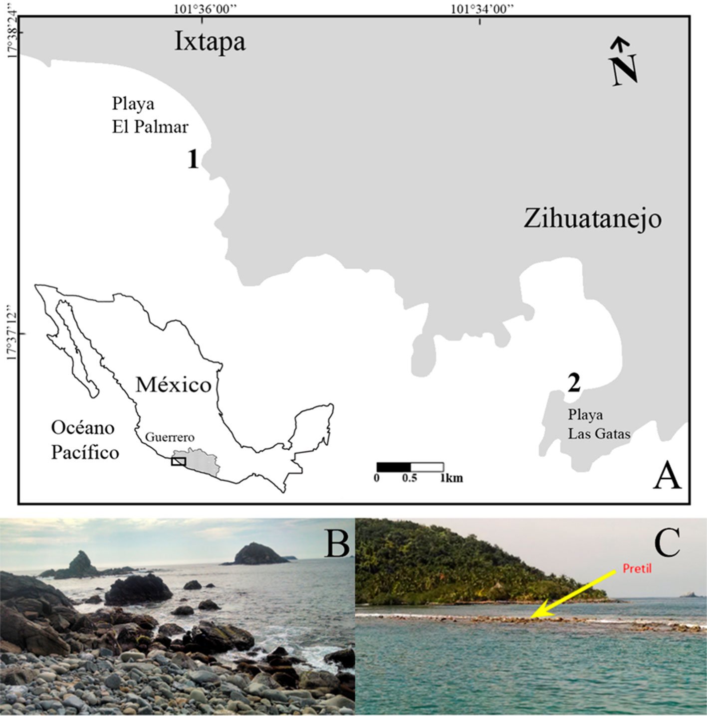
Figura 1. A, Ubicación de la zona de estudio en Ixtapa-Zihuatanejo; B, playa El Palmar; C, playa Las Gatas.
En cada localidad, 3 muestras de macroalgas se recolectaron manualmente de forma aleatoria con una espátula (Bakus, 2007), dentro de cuadros de 20 × 20 cm (0.04 m2) por cada nivel de marea: intermareal bajo (3), medio (3) y alto (3); en total, se obtuvieron 72 muestras provenientes de 36 cuadros en playa Las Gatas y de 36 cuadros en playa El Palmar. Las muestras de las comunidades de macroalgas y moluscos asociados se preservaron en una mezcla de formaldehído al 4% con agua de mar, neutralizada con borato de sodio y glicerina; después se trasladaron al Laboratorio de Ficología (Biodiversidad Marina) de la Facultad de Ciencias de la Universidad Nacional Autónoma de México (UNAM).
En el laboratorio, se calculó la cobertura de cada especie de macroalga en cm2 al colocar cada muestra sobre un área delimitada de 20 × 20 cm. Para su identificación taxonómica se tomaron en cuenta las características morfológicas externas, como tipo de talo y tipo de ramificación, e internas a partir de cortes anatómicos transversales de ejes, frondas y, de estar presentes, de estructuras reproductivas; los especímenes y cortes fueron observados bajo microscopios estereoscópico y óptico (Zeiss). La identificación taxonómica de los ejemplares de macroalgas se realizó utilizando literatura especializada para macroalgas del océano Pacífico (Abbott, 1999; Abbott y Hollenberg, 1976; Dawson, 1949, 1953, 1954, 1960, 1961, 1963; Dawson y Beaudette, 1959; Rodríguez et al.,2008; Taylor, 1945). La actualización de la nomenclatura se hizo a partir de la base de datos de Algaebase (Guiry y Guiry, 2024) y, con base en ella, se elaboró una lista sistemática de las especies de macroalgas. De cada comunidad de macroalgas se separó el sedimento retenido por las algas después de la medición de la cobertura para cada especie y se midió su peso húmedo con una balanza digital, modelo OBI.
De cada muestra, se extrajeron de forma manual todos los moluscos de la clase Bivalvia. Los ejemplares con concha y parte blanda (vivos) fueron identificados al nivel taxonómico más bajo posible, género o especie, dependiendo del estado de conservación de cada ejemplar, a partir de la observación de las características morfológicas de la concha, con apoyo de un microscopio estereoscópico. La identificación taxonómica de las especies se hizo con literatura malacológica especializada para la zona del océano Pacífico oriental (Coan et al., 2000; Keen, 1971). Se elaboró una lista sistemática con base en la propuesta de Bouchet et al. (2010) para los niveles suprafamiliares y la actualización de nomenclatura se realizó a partir de la base de datos de World Register of Marine Species (WORMS) para género y especie (Horton et al., 2024).
Los ejemplares de moluscos y macroalgas recolectados fueron depositados en la colección “Invertebrados asociados a macroalgas”, en proceso de registro, con número de inventario para bivalvos (INV-1531 a INV-1638) del Laboratorio de Ficología (Biodiversidad Marina) de la Facultad de Ciencias, UNAM y las macroalgas se depositaron en la colección del Herbario de la Facultad de Ciencias (FCME) con número de catálogo (PTM-10534 a PTM-10558; PTM-10577 a PTM-10604; PTM-10613 a PTM-10630; PTM-10640 a PTM-10648).
Se elaboró una curva de acumulación de las especies de bivalvos asociados a macroalgas recolectadas en las localidades de estudio, con la finalidad de conocer la cantidad de especies que faltaría encontrar y recolectar en dichas localidades. Con los datos de riqueza de especies (S) y abundancia de bivalvos (N) de ejemplares vivos (concha y parte blanda), se estimaron los índices de Shannon (H´) y de diversidad máxima (H’ max) para cada fecha de muestreo, ya que éstos corresponden a los miembros de la comunidad en el momento de muestreo (Aguilar-Estrada et al., 2014); H´ fue expresado en bits/individuo (Magurran, 2004). Se calculó el índice de equidad de Pielou (J´) y el índice de dominancia de Simpson (D) (Moreno, 2001). Estos índices permiten hacer comparaciones cuantitativas y cualitativas entre estudios o zonas ya que se han utilizado como referente mínimo para describir la estructura comunitaria de un lugar (Aguilar-Estrada et al., 2014).
Para evaluar la normalidad de los datos de abundancia de bivalvos y de los índices de diversidad se realizaron pruebas de Shapiro-Wilk (W) (Siegel, 1990). Posteriormente, se realizaron pruebas de Levene (F) para comprobar la homogeneidad de varianzas para los datos no normales y prueba de Bartlett para los datos con distribución normal (Bartlett, 1937; Levene, 1960). Los índices de diversidad de Shannon fueron analizados usando una prueba de “t de student” para evaluar si existían diferencias estadísticamente significativas entre los meses de muestreo. Estos análisis se realizaron utilizando la paquetería Vegan Versión 2.5-6 (Oksanen et al., 2019) en el programa R Studio 2023.12.0+369 (R Core Team, 2023).
Los datos de abundancia de bivalvos no fueron normales de acuerdo con las pruebas de normalidad, por ello, se realizaron análisis de estadística no paramétrica en el software PRIMER v6 + add on Permanova (PRIMER-E Ltd., Plymouth, UK) (Anderson et al., 2008; Clarke y Gorley, 2006). Los datos fueron transformados con 4√ y con ellos se calculó una matriz de similitud a partir del índice de Bray-Curtis. A partir de dicha matriz, se realizó un análisis de escalamiento multidimensional no métrico (nMDS) con la finalidad de observar la distribución de las abundancias de bivalvos en el área de estudio. Se incluyó la abundancia de las especies dominantes en forma de vectores azules superpuestos en el gráfico nMDS para facilitar la interpretación de las abundancias de especies dominantes en las distintas localidades y niveles de marea, donde el círculo azul representa la variación de la abundancia. Las especies dominantes que se seleccionaron en este análisis son las que estuvieron presentes en todas las muestras con abundancias mayores a la media.
Además, se realizaron análisis de varianza permutacionales (Permanova) para determinar si existían diferencias significativas en la abundancia de bivalvos (variable dependiente) con respecto a los factores utilizados: localidad con 2 niveles (El Palmar y Las Gatas), nivel de marea con 3 niveles (alto, medio y bajo) y mes de muestreo con 4 niveles (enero, mayo, julio y noviembre). En los análisis de Permanova se utilizaron 999 permutaciones de los residuos bajo un modelo reducido. Posteriormente, para los factores donde se obtuvieron diferencias significativas, se realizaron comparaciones de pares para identificar los niveles que eran diferentes estadísticamente (Anderson et al., 2008).
Utilizando las variables numéricas, se realizaron regresiones lineales múltiples con el software SPSS Statistics v20, para evaluar el efecto de la cobertura de macroalgas y los sedimentos retenidos (variables independientes) en la abundancia de bivalvos (variable dependiente) en las playas El Palmar y Las Gatas, en los diferentes niveles de marea y en los meses de muestreo.
Por último, se determinó el grupo morfofuncional (GMF): filamentosas (Fil), foliosas (Fol), foliosas corticadas (Foc), filamentosas corticadas (Fic), coriáceas (Cor), calcáreas articuladas (Cal) para cada especie de macroalgas, con base en la propuesta de Steneck y Dethier (1994) y se asociaron con las especies de bivalvos recolectadas.
Resultados
Riqueza y composición de moluscos. En 60 de las 72 muestras recolectadas se encontraron bivalvos, 35 muestras pertenecientes a playa El Palmar y 25 a playa Las Gatas. Se obtuvieron un total de 873 individuos de la clase Bivalvia. Se identificaron 17 especies (fig. 2) agrupadas en 2 subclases, 8 órdenes, 10 familias y 15 géneros. Del total de especies recolectadas, 2 de ellas Parvilucina approximata (Dall, 1901) y Pinna rugosa G. B. Sowerby I, 1835, encontradas en playa El Palmar y playa Las Gatas, respectivamente, no se incluyeron en los análisis de estructura comunitaria, dado que solo se recolectó la concha. Se obtuvieron 13 especies en playa El Palmar y 9 en playa Las Gatas. Las familias Carditidae y Mytilidae fueron las mejor representadas con 3 (18%) y 5 (30%) especies, respectivamente.
En ambas localidades, las especies más abundantes fueron: Brachidontes adamsianus (Dunker, 1857), Leiosolenus aristatus (Dillwyn, 1817) e Isognomon janus Carpenter, 1857, con 376, 205 y 124 individuos, respectivamente, lo cual representó 91% del total de individuos. Brachidontes adamsianus obtuvo la mayor abundancia en El Palmar a lo largo del ciclo anual, con el valor más elevado (161 individuos) en enero. En Las Gatas, Leiosolenus aristatus fue la especie con la mayor abundanciacon 140 individuos en enero; sin embargo, la especie más abundante fue B. adamsianus a lo largo de los otros meses de muestreo. Mientras que las especies menos abundantes fueron: Sphenia fragilis (H. Adams & A. Adams, 1854) con 2 individuos en enero y mayo en El Palmar y 1 individuo en noviembre en Las Gatas, Crassinella ecuadoriana Olsson, 1961 con 2 individuos en mayo y julio en El Palmar, Linucula declivis (Hinds, 1843) con 2 individuos en julio y noviembre en Las Gatas, Mya sp. y Mytilus edulis Linnaeus, 1758 con 1 individuo en enero en El Palmar (tabla 1).
Tabla 1
Abundancia de las especies de bivalvos recolectadas en las localidades de estudio por mes de muestreo. El arreglo sistemático sigue la propuesta de Horton et al. (2024).
| Especie | Playa El Palmar | Playa Las Gatas | |||||||
| ene | may | jul | nov | ene | may | jul | nov | Total | |
| Subclase Protobranchia | |||||||||
| Orden Nuculida | |||||||||
| Familia Nuculidae | |||||||||
| Linucula declivis | – | – | – | – | – | – | 1 | 1 | 2 |
| Subclase Autobranchia | |||||||||
| Orden Mytilida | |||||||||
| Familia Mytilidae | |||||||||
| Brachidontes adamsianus | 161 | 43 | 18 | 14 | 41 | 9 | 34 | 56 | 376 |
| Brachidontes semilaevis | 4 | – | – | 1 | – | – | – | – | 5 |
| Leiosolenus aristatus | 2 | 30 | 1 | 6 | 140 | 7 | 5 | 14 | 205 |
| Modiolus capax | 1 | 2 | 1 | 1 | – | – | – | – | 5 |
| Mytilus edulis | 1 | – | – | – | – | – | – | – | 1 |
| Orden Arcida | |||||||||
| Familia Arcidae | |||||||||
| Acar rostae | – | – | – | – | – | – | 1 | 3 | 4 |
| Orden Ostreida | |||||||||
| Familia Pteriidae | |||||||||
| Isognomon janus | 51 | 32 | 8 | 5 | 2 | – | 10 | 16 | 124 |
| Familia Pinnidae | |||||||||
| Pinna rugosa | – | – | – | – | – | – | 3 | – | 3 |
| Orden Lucinida | |||||||||
| Familia Lucinidae | |||||||||
| Parvilucina approximata | 1 | – | – | – | – | – | – | – | 1 |
| Orden Carditida | |||||||||
| Familia Carditidae | |||||||||
| Carditamera affinis | 5 | 2 | – | – | 1 | – | – | 1 | 9 |
| Carditamera radiata | – | 3 | 1 | – | 3 | – | 3 | 5 | 15 |
| Cardites grayi | – | 1 | 3 | – | – | – | – | – | 4 |
| Familia Crassatellidae | |||||||||
| Crassinella ecuadoriana | – | 1 | 1 | – | – | – | – | – | 2 |
| Orden Venerida | |||||||||
| Familia Chamidae | |||||||||
| Chama coralloides | 3 | 2 | 1 | – | – | – | – | 7 | 13 |
| Orden Myida | |||||||||
| Familia Myidae | |||||||||
| Mya sp. | 1 | – | – | – | – | – | – | – | 1 |
| Sphenia fragilis | 1 | 1 | – | – | – | – | – | 1 | 3 |
| Total | 231 | 117 | 34 | 27 | 187 | 16 | 57 | 104 | 773 |
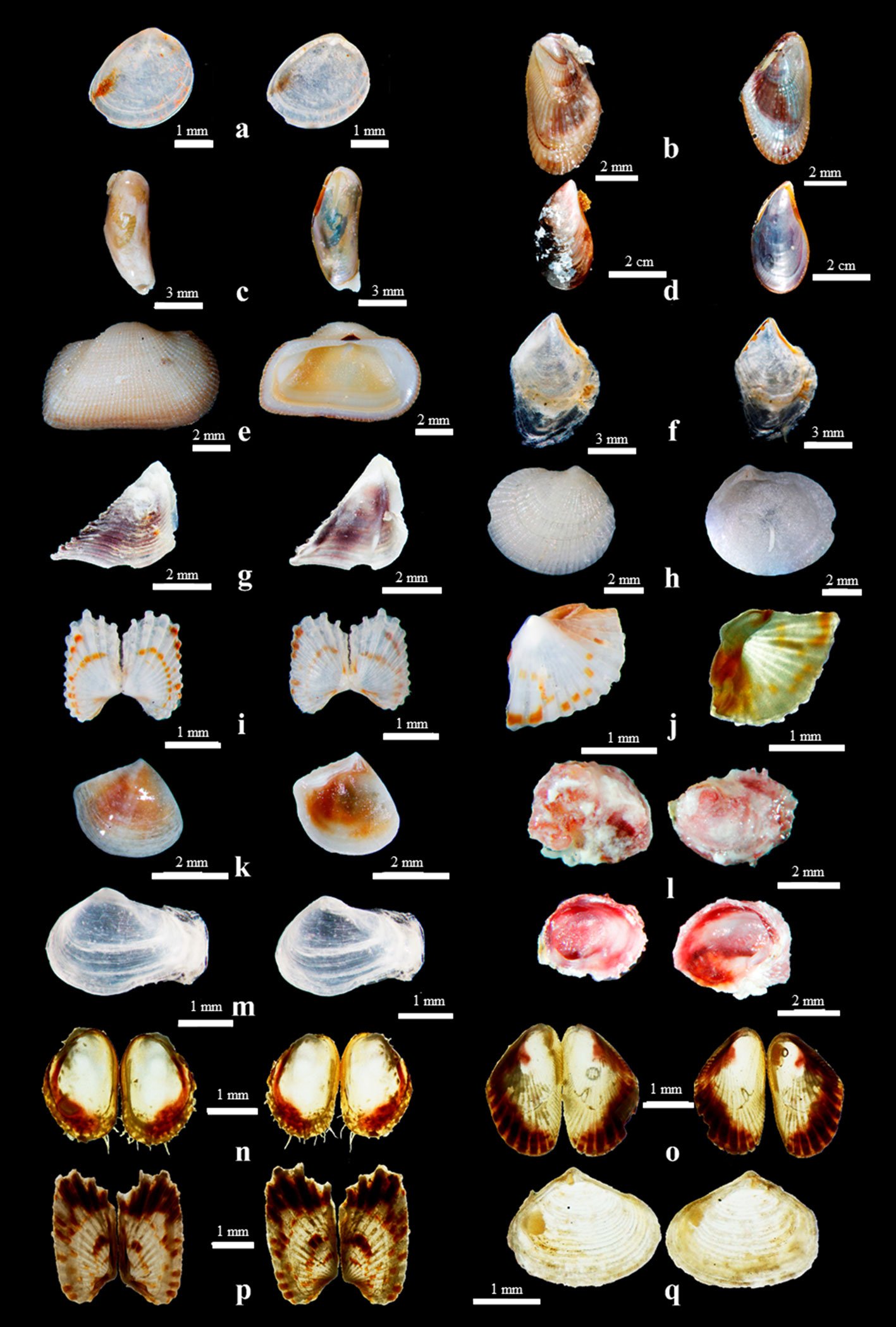
Figura 2. Especies de bivalvos asociadas a macroalgas recolectadas en Ixtapa-Zihuatanejo, Guerrero, en vista dorsal y ventral. a, Linucula declivis;b, Brachidontes adamsianus;c, Leiosolenus aristatus; d, Mytilus edulis; e, Acar rostae; f, Isognomon janus;g, Pinna rugosa; h, Parvilucina approximata; i, Carditamera radiata; j, Cardites grayi; k, Crassinella ecuadoriana; l, Chama coralloides;m, Sphenia fragilis; n, Modiolus capax;o, Brachidontes semilaevis;p, Carditamera affinis;q, Mya sp.
La riqueza de especies con relación al ciclo anual fue de 13 especies en playa El Palmar, variando entre 5 (noviembre) y 10 especies (enero) a lo largo de los meses, mientras que en playa Las Gatas se obtuvieron 9 especies, con una variación de 2 (mayo) y 9 (noviembre) especies (tabla 1). La curva de acumulación de especies mostró un comportamiento asintótico en El Palmar, mientras que Las Gatas no mostró una tendencia a ser asintótica (fig. 3).
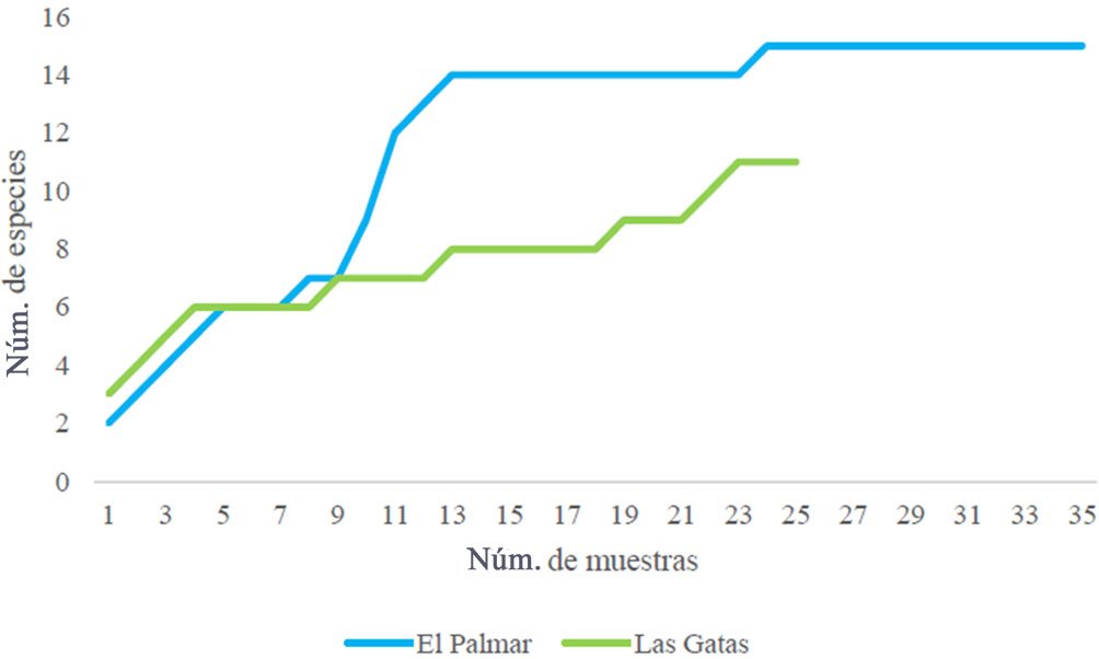
Figura 3. Curva de acumulación de especies de bivalvos registrados en las localidades de estudio. Línea azul: playa El Palmar, línea verde: playa Las Gatas.
En playa El Palmar el nivel intermareal bajo obtuvo el mayor número de especies (13) y el menor número de especies se presentó tanto en el nivel intermareal medio como en el alto (7); mientras que en playa Las Gatas, se presentó el mayor número de especies en el nivel intermareal medio (10) y el nivel alto tuvo el menor número de especies (5). Las especies que se presentaron en ambas localidades en los 3 niveles de la zona intermareal fueron Brachidontes adamsianus, Leiosolenus aristatus e Isognomon janus.
En El Palmar se registraron valores del índice de diversidad de Shannon que fluctuaron entre 1.30 y 2.15 bits/individuo, mientras que en Las Gatas este índice varió entre 0.98 y 2.09 bits/individuo (tabla 2). En general, el índice de equidad de Pielou presentó valores mayores a 0.60 en playa El Palmar, excepto en enero, mientras que en playa Las Gatas se observó que los valores fueron bajos en enero y mayo, y mayores a 0.60 en julio y noviembre. Las pruebas de “t de student”para el índice de diversidad de Shannon entre los meses de muestreo, indicaron diferencias significativas entre todos ellos (p ≤ 0.05) en El Palmar, y Las Gatas (tabla 3).
Tabla 2
Índices comunitarios calculados para las especies recolectadas en playa El Palmar y playa Las Gatas. N = número de individuos, H’= Índice de Shannon, J’= equidad de Pielou y λ = dominancia de Simpson. Los valores máximos y mínimos por localidad para el índice de Shannon (H´) se marcan con negritas.
| Playa El Palmar | Playa Las Gatas | |||||||
| Mes | N | H’ | J’ | λ | N | H’ | J’ | λ |
| Enero | 230 | 1.30 | 0.48 | 0.54 | 187 | 0.99 | 0.41 | 0.60 |
| Mayo | 117 | 2.15 | 0.81 | 0.27 | 16 | 0.98 | 0.41 | 0.50 |
| Julio | 34 | 2.03 | 0.77 | 0.34 | 54 | 1.63 | 0.68 | 0.44 |
| noviembre | 27 | 1.77 | 0.67 | 0.35 | 104 | 2.09 | 0.87 | 0.33 |
En el análisis de escalamiento multidimensional no métrico (nMDS), a partir de los valores de abundancia de las especies de bivalvos, se observó que las muestras se separan en 3 grupos: un primer grupo dominado por estaciones pertenecientes a playa El Palmar (P), un segundo grupo principalmente con estaciones de playa Las Gatas (G) y uno tercero con estaciones de ambas localidades que probablemente se separa por la dominancia de la especie Brachidontes adamsianus (fig. 4). El vector indica la dirección a través del plano de ordenación en la cual aumentan los valores de abundancia de las especies dominantes, la longitud de la línea indica la cantidad de variación total de cada especie, entonces, si toda la variación se explicara, la línea azul alcanzaría el círculo azul.
Tabla 3
Resultado de la prueba de “t de student”para evaluar diferencias significativas del índice de Shannon entre los meses de muestreo por localidad.
| Playa El Palmar | Playa Las Gatas | |||||||
| Meses | H´ | t | p | gl | H´ | t | p | gl |
| enero vs. mayo | 1.30/2.15 | -0.009 | 324 | 1 | 0.99/0.98 | 0.009 | 169 | 1 |
| mayo vs. julio | 2.15/2.03 | 0.0004 | 142 | 0.98/1.63 | -19.84 | 4 | ||
| julio vs. noviembre | 2.03/1.17 | 0.023 | 60 | 1.63/2.09 | -3.18 | 94 |
El análisis de Permanova reveló que la composición de bivalvos difiere significativamente entre las diferentes localidades muestreadas (pseudo-F = 5.2373, p = 0.001). No hubo diferencias estadísticamente significativas para los meses de muestreo (pseudo-F=1.431, p = 0.147) y el nivel de marea (pseudo-F = 1.19, p = 0.309) (tabla 4).
Tabla 4
Resultado de los análisis de Permanova para los factores de localidad, mes de muestreo y nivel de marea. GL: Grados de libertad, ms: media suma de cuadrados, perm: permutaciones, * = valores significativos.
| Factor | GL | ms | Pseudo-F | p (perm) |
| Localidad | 1 | 7,844.9 | 5.2373 | 0.001* |
| Res | 57 | 1,497.9 | ||
| Total | 58 | |||
| Mes | 3 | 2,249.9 | 1.431 | 0.147 |
| Res | 55 | 1,572.3 | ||
| Total | 58 | |||
| Nivel de marea | 2 | 1,915 | 1.1996 | 0.309 |
| Res | 56 | 1,596.3 | ||
| Total | 58 |
Riqueza y composición de macroalgas. Se encontró un total de 3 phyla, 3 clases, 5 subclases, 14 órdenes, 20 familias, 33 géneros y 59 especies de macroalgas; de las cuales, a cada localidad le pertenecen 37 especies. De las 59 especies totales, 11 fueron Chlorophyta (18%), 42 Rhodophyta (70%) y 7 Heterokontophyta-Phaeophyceae (11%). Entre ambas localidades se compartieron 16 especies. Las familias con mayor número de especies fueron Rhodomelaceae con 12 especies, Corallinaceae con 10 y Ceramiaceae y Dictyotaceae con 5 especies cada una (tabla 5).
Asociación entre grupos morfofuncionales y moluscos. Las macroalgas se clasificaron en 6 grupos morfofuncionales: algas filamentosas, foliosas, foliosas corticadas, filamentosas corticadas, coriáceas y calcáreas articuladas (tabla 5). Los grupos dominantes en las 2 localidades fueron las algas filamentosas, filamentosas corticadas y las calcáreas articuladas. En playa El Palmar se presentó una mayor riqueza de especies (14) de bivalvos al interior de las comunidades algales que contenían el grupo de algas calcáreas articuladas. En playa Las Gatas, los grupos morfofuncionales que presentaron mayor cantidad de especies fueron las algas filamentosas, filamentosas corticadas y las calcáreas articuladas con 10 especies cada uno (tabla 6).
Cobertura de macroalgas, abundancia de moluscos y sedimentos retenidos. La regresión lineal por localidad indicó que para playa El Palmar hay una correlación baja con 24% entre los componentes: cobertura de macroalgas, abundancia de bivalvos y peso de sedimento húmedo; sin embargo, se observó una relación moderada entre los sedimentos retenidos por las macroalgas y la abundancia de bivalvos (R = 0.55 y R2 = 0.24). Para playa Las Gatas la regresión lineal múltiple indicó una correlación baja con 10% entre los factores y una relación moderada entre la cobertura de macroalgas y la abundancia de bivalvos (R = 0.42 y R2 = 0.10). La cobertura de macroalgas, abundancia de bivalvos y los sedimentos retenidos varió según la localidad (fig. 5A-C), mes de muestreo (fig. 5D-F) y nivel de marea (fig. 5G-I). En El Palmar la regresión lineal mostró una relación directamente proporcional entre la abundancia de bivalvos y la cobertura de macroalgas. Los valores más altos de cobertura de macroalgas (0.89 m2) se relacionaron con los valores más altos de abundancia de bivalvos.
Con respecto al mes de muestreo, las regresiones lineales múltiples indicaron una correlación alta con 98% (R = 0.99 y R2 = 0.98), entre la cantidad de sedimento retenido y la abundancia de bivalvos. La regresión lineal múltiple sugirió que la abundancia de bivalvos disminuyó a lo largo del ciclo anual, donde enero presentó la mayor abundancia (de 187-230 individuos) y noviembre la menor (27 individuos). La relación de la abundancia de bivalvos con el peso húmedo de sedimento tuvo un comportamiento parecido, disminuyendo conforme al ciclo anual: en las muestras de enero se reportó mayor sedimento retenido (0.56 kg), mientras que en julio se encontraron menos sedimentos retenidos (0.17 kg).

Figura 4. Análisis de escalamiento multidimensional no métrico (nMDS) de las especies de bivalvos recolectadas en las localidades de estudio. Las líneas azules (vectores) indican las especies abundantes y frecuentes (dominantes). El círculo azul representa la variación de las abundancias.
Tabla 5
Especies de macroalgas asociadas a bivalvos, para cada localidad y grupo morfofuncional. Se marca con * la especie de macroalga presente en la localidad. Localidad: playa El Palmar (P), playa Las Gatas (G). Grupos morfofuncionales de macroalgas: filamentosas (Fil), foliosas (Fol), foliosas corticadas (Foc), filamentosas corticadas (Fic), coriáceas (Cor), calcáreas articuladas (Cal). Especies de bivalvos: 1) Linucula declivis, 2) Brachidontes adamsianus, 3) Brachidontes semilaevis, 4) Leiosolenus aristatus, 5) Modiolus capax, 6) Mytilus edulis, 7) Acar rostae, 8) Isognomon janus, 9) Carditamera affinis, 10) Carditamera radiata, 11) Cardites grayi, 12) Crassinella ecuadoriana, 13) Chama coralloides, 14) Mya sp., 15) Sphenia fragilis,16) Pinna rugosa, 17) Parvilucina approximata.
| Especies | Grupo morfofuncional | Especies de bivalvos | |
| P | G | ||
| Chlorophyta | |||
| Ulvales | |||
| Ulvaceae | |||
| Ulva californica Wille, 1899 | Fol | * | – |
| Ulva intestinalis Linnaeus, 1753 | Fol | – | 2, 4, 13 |
| Ulva linza Linnaeus, 1753 | Fol | – | 2, 4, 13 |
| Bryopsidales | |||
| Bryopsidaceae | |||
| Bryopsis pennata var. minor J. Agardh, 1887 | Fil | – | 2, 4, 8 |
| Caulerpaceae | |||
| Caulerpa chemnitzia (Esper) J.V. Lamouroux, 1809 | Fil | 2, 4, 8, 10, 17 | 1, 2, 4, 7, 8, 9, 10, 15 |
| Caulerpa sertularioides (S.G. Gmelin) M. Howe, 1905 | Fil | 2, 4, 8, 10, 17 | 1, 2, 4, 7-10, 15 |
| Halimedaceae | |||
| Halimeda discoidea Decaisne, 1842 | Cal | 2, 10, 17 | – |
| Cladophorales | |||
| Cladophoraceae | |||
| Chaetomorpha antennina (Bory) Kützing, 1847 | Fil | 2, 3, 7, 8-13 | 4, 7, 8, 11, 13 |
| Cladophora sp. | Fil | 2, 4, 5, 8, 9 | – |
| Cladophora graminea Collins, 1909 | Fil | – | 16 |
| Cladophora microcladioides Collins, 1909 | Fil | 2, 4, 5, 8, 9 | – |
| Rhodophyta | |||
| Gigartinales | |||
| Cystocloniaceae | |||
| Hypnea pannosa J. Agardh, 1847 | Fic | 2-6, 8-15 | 2, 4, 8-10, 16 |
| Hypnea spinella (C. Agardh) Kützing, 1847 | Fic | 2-6, 8-15, 17 | 2, 4, 8-10, 16 |
| Hypnea johnstonii Setchell y N. L. Gardner, 1924 | Fic | – | 1, 2, 4, 7-10, 16 |
| Phyllophoraceae | |||
| Ahnfeltiopsis gigartinoides (J. Agardh) P. C. Silva y DeCew, 1992 | Fic | 8 | – |
| Gymnogongrus johnstonii (Setchell y N. L. Gardner) E.Y. Dawson, 1961 | Fic | 2, 8 | – |
| Ceramiales | |||
| Ceramiaceae | |||
| Centroceras clavulatum (C. Agardh) Montagne, 1846 | Fil | 2-5, 8 | 2, 4, 10, 15 |
| Tabla 5. Continúa | |||
| Especies | Grupo morfofuncional | Especies de bivalvos | |
| P | G | ||
| Ceramium sp. | Fil | – | 1, 2, 4, 7, 8, 10, 13, 16 |
| Ceramium camouii E. Y. Dawson, 1944 | Fil | – | 1, 2, 4, 7, 8, 10, 13, 16 |
| Ceramium zacae Setchell y N. L. Gardner, 1937 | Fil | – | 1, 2, 4, 7, 8, 10, 13, 16 |
| Gayliella flaccida (HarveyyKützing) T.O. McIvory y L.J. Cho, 2008 | Fic | – | 2, 4, 7, 8, 11 |
| Delesseriaceae | |||
| Taenioma perpusillum (J. Agardh) J. Agardh, 1863 | Fil | – | 4, 16 |
| Rhodomelaceae | |||
| Chondria sp. | Fic | * | * |
| Herposiphonia secunda (C. Agardh) Ambronn, 1880 | Fic | 8 | 2, 4, 8, 10 |
| Herposiphonia tenella (C. Agardh) Ambronn, 1880 | Fic | 7 | – |
| Melanothamnus simplex (Hollenberg) Díaz-Tapia y Maggs, 2017 | Fic | 2, 8 | – |
| Melanothamnus sphaerocarpus (Borgesen) Díaz.Tapioa y Maggs, 2017 | Fic | – | 2, 4, 8 |
| Polysiphonia mollis J. D. Hooker y Harvey, 1847 | Fic | * | 2, 4, 8, 15 |
| Polysiphonia nathanielii Hollenberg, 1958 | Fic | – | 2, 4, 8, 15 |
| Polysiphonia subtilissima Montagne, 1840 | Fic | – | 2, 4, 8, 15 |
| Eutrichosiphonia confusa (Hollenberg) Savoie y G.W. Saunders, 2019 | Fic | – | 2, 4, 8 |
| Laurencia sp. | Fic | 2, 8, | 2, 7, 8, 13 |
| Laurencia hancockii E.Y. Dawson, 1944 | Fic | 2, 8 | – |
| Laurencia subcorymbosa E.Y. Dawson, 1963 | Fic | 2, 8 | – |
| Rhodymeniales | |||
| Rhodymeniaceae | |||
| Tayloriella dictyurus (J. Agardh) Kylin, 1956 | Fil | 2, 8 | – |
| Lomentariaceae | |||
| Ceratodictyon tenue (Setchell y N. L. Gardner) J.N. Norris, 2014 | Fil | – | 2, 4, 8 |
| Corallinales | |||
| Corallinaceae | |||
| Amphiroa beauvoisii J.V. Lamouroux, 1816 | Cal | 2-15, 17 | 1, 2, 4, 7-14, 16 |
| Amphiroa misakiensis Yendo, 1902 | Cal | 2-15 | 1, 2, 4, 7-14, 16 |
| Amphiroa rigida J.V. Lamouroux, 1816 | Cal | 2-15 | 1, 2, 4, 7-14, 16 |
| Amphiroa subcylindrica E.Y. Dawson, 1953 | Cal | 2-15 | – |
| Jania capillacea Harvey, 1853 | Cal | – | 2, 4, 7-10, 15, 16 |
| Jania subpinnata E.Y. Dawson, 1953 | Cal | 2, 4, 5, 8, 9, 12, 14 | 2, 4, 7-10, 15, 16 |
| Jania tenella (Kützing) Grunow, 1874 | Cal | 2, 4, 5, 8, 9, 12, 14 | 2, 4, 7-10, 15, 16 |
| Jania tenella var. tenella | Cal | 2, 4, 5, 8, 9, 12, 14 | – |
| Gelidiales | |||
| Gelidiaceae | |||
| Gelidiella acerosa (Forsskal) Feldmann y Hamel, 1934 | Fic | – | 2, 7, 8 |
| Gelidium mcnabbianum (E.Y. Dawson) B. Santelices, 1998 | Fic | – | 2, 4, 7-11 |
| Gelidium pusillum (Stackhouse) Le Jolis, 1863 | Fic | 2, 4, 5, 8, 12, 14 | 2, 4, 7-11 |
| Pterocladiaceae | |||
| Pterocladiella caloglossoides (M. Howe) Santelices, 1998 | Fic | – | 2, 4, 7, 8, 15 |
| Gracilariales | |||
| Gracilariaceae | |||
| Gracilaria sp. | Fic | 2, 8, 12, 14 | – |
| Halymeniales | |||
| Halymeniaceae | |||
| Grateloupia huertana Mateo-Cid, Mendoza-González y Gavio, 2005 | Fic | – | 4, 8 |
| Grateloupia versicolor (J. Agardh) J. Agardh, 1847 | Fic | 2, 4, 8 | – |
| Heterokontophyta-Phaeophyceae | |||
| Ectocarpales | |||
| Scytosiphonaceae | |||
| Chnoospora minima Papenfuss, 1956 | Fic | * | – |
| Fucales | |||
| Sargassaceae | |||
| Sargassum liebmannii Agardh, 1847 | Cor | 2, 4, 5, 7, 8, 10-13, 15, 17 | – |
| Dictyotales | |||
| Dictyotaceae | |||
| Dictyota sp. | Foc | – | * |
| Dictyota dichotoma (Hudson) J.V. Lamouroux, 1809 | Foc | 2, 4, 5, 8 | – |
| Lobophora variegata (J.V.Lamouroux)Womersley ex E.C.Oliveira, 1977 | Fic | 8 | – |
| Padina mexicana var. erecta Avila-Ortiz, 2003 | Foc | 2, 4, 5, 8, 9 | – |
| Padina ramonribae Avila-Ortiz, Pedroche y Díaz-Martínez, 2016 | Foc | 2, 4, 5, 8, 9 | – |
La regresión lineal por nivel de marea indicó una correlación significativa con 100% (R = 1 y R2 = 1), es decir, la cobertura de algas y el sedimento retenido están relacionados con la abundancia de bivalvos en los diferentes niveles de marea. El nivel del intermareal bajo presentó los valores más elevados de cobertura de macroalgas con 0.61 m2 (fig. 5G), mayor abundancia de moluscos con 275 individuos (fig. 5H) y mayor cantidad de sedimentos con 0.69 kg (fig. 5I). En el intermareal alto se registraron los valores más bajos de abundancia de bivalvos con 230 individuos (fig. 5H), cobertura de algas con 0.52 m2 (fig. 5G) y peso húmedo de sedimentos con 0.30 kg (fig. 5I), es decir, conforme se asciende en el intermareal, estas variables disminuyen.
Tabla 6
Asociación de las especies de bivalvos con los grupos morfofuncionales propuestos por Steneck y Dethier (1994). Grupos morfofuncionales de macroalgas: filamentosas (Fil), foliosas (Fol), foliosas corticadas (Foc), filamentosas corticadas (Fic), coriáceas (Cor), calcáreas articuladas (Cal). × = Presencia de la especie.
| Familia | Especie | Playa El Palmar | Playa Las Gatas | ||||||||||
| Fil | Fol | Foc | Fic | Cor | Cal | Fil | Fol | Foc | Fic | Cor | Cal | ||
| Nuculidae | L. declivis | – | – | – | – | – | – | × | – | – | × | – | × |
| Mytilidae | B. adamsianus | × | – | × | × | × | × | × | × | – | × | – | × |
| B. semilaevis | × | – | – | × | – | × | – | – | – | – | – | – | |
| L. aristatus | × | – | × | × | × | × | × | × | – | × | – | × | |
| M. capax | × | – | × | × | × | × | – | – | – | – | – | – | |
| M. edulis | – | – | – | × | – | × | – | – | – | – | – | – | |
| Arcidae | A. rostae | × | – | – | – | × | × | × | – | – | × | – | × |
| Pteriidae | I. janus | × | – | × | × | × | × | × | – | – | × | – | × |
| Pinnidae | P. rugosa | – | – | – | – | – | – | × | – | – | × | – | × |
| Lucinidae | P. approximata | × | – | – | × | × | × | – | – | – | – | – | – |
| Carditidae | C. affinis | × | – | × | × | – | × | × | – | – | × | – | × |
| C. radiata | × | – | – | × | × | × | × | – | – | × | – | × | |
| C. grayi | × | – | – | × | × | × | × | – | – | × | – | × | |
| Crassatellidae | C. ecuadoriana | × | – | – | × | × | × | – | – | – | – | – | – |
| Chamidae | C. coralloides | × | – | – | × | × | × | × | × | – | × | – | × |
| Myidae | Mya sp. | – | – | – | × | – | × | – | – | – | – | – | – |
| S. fragilis | – | – | – | × | × | × | × | – | – | × | – | × | |
| Total | 12 | 0 | 5 | 14 | 11 | 15 | 11 | 3 | 0 | 11 | 0 | 11 |
Discusión
Riqueza y composición de moluscos. De las 17 especies encontradas en el presente estudio, 16 ya habían sido observadas para el Pacífico tropical mexicano, específicamente para Ixtapa-Zihuatanejo en sustratos rocosos y arenosos (Flores-Rodríguez et al., 2007, 2012; Lesser, 1984; López-Rojas et al.,2017; Lozada, 2010; Sánchez, 2014), excepto Mytilus edulis que es un nuevo registro para Guerrero. Esta especie fue encontrada en playa El Palmar, asociada a los géneros de macroalgas Amphiroa e Hypnea. Dicha especie había sido registrada para el océano Pacífico desde las costas del Ártico, Canadá, EUA, hasta Cabo San Lucas, México, al interior del golfo de California en San Luquitas y Santa Rosalía, y para el Pacífico tropical mexicano en isla Socorro, por lo que su distribución se amplía hacia el sur, a Guerrero en ambientes litorales asociados a las comunidades de macroalgas (Cadena-Cárdenas et al., 2009; Fitch, 1953; Shaw et al., 1988). La ampliación de la distribución de esta especie puede deberse al movimiento de la corriente de California como ha sido reportado para bivalvos (Schulien et al., 2020), gasterópodos y escafópodos que ampliaron su distribución desde la provincia Californiana hacia la Panámica donde se señala la confluencia de especies de moluscos entre ambas provincias (Landa-Jaime y Arciniega-Flores 1998; Ríos-Jara et al., 2003; Gama-Kwick et al., 2021). Otra de las razones por la cual M. edulis amplió su distribución al sur podría ser por el fenómeno de El Niño que proporciona condiciones ambientales para que las especies que habitan en sitios templados y subtropicales se desplacen a sitios tropicales (Díaz y Ortlieb, 1993; Paredes et al., 1998; Velez y Zeballos, 1985).

Figura 5. Variación de cobertura de macroalgas, abundancia de bivalvos y sedimento retenido por localidades (A, B y C), mes de muestreo (D, E y F) y nivel de la zona intermareal (G, H e I). Verde = macroalgas, amarillo = bivalvos, rojo = sedimento retenido.
La familia mejor representada fue Mytilidae con 5 especies: Brachidontes adamsianus, B. semilaevis, Leiosolenus aristatus, Modiolus capax y Mytilus edulis (tabla 1), dichas especies coinciden con lo registrado por Flores-Garza et al.(2014), Galeana-Rebolledo et al.(2012) y Garcés (2011) en Acapulco, así como por López-Rojas et al. (2017) en diferentes localidades en Guerrero. Mytilidae también ha sido la familia mejor representada en otras localidades de Zihuatanejo (muelle municipal), donde se han observado 8 especies (Guzmán, 2022), así como en otras regiones tropicales como Brasil, donde esta familia también fue la mejor representada con 5 especies (Santos et al., 2020).
Una mayor riqueza de especies de la familia Mytilidae en Ixtapa-Zihuatanejo podría explicarse debido a la frecuencia y rápido asentamiento de larvas de bivalvos, ya que son organismos que están en constante reproducción a lo largo del año (Seed, 1969a). Suchanek (1978) mencionó que los miembros de la familia Mytilidae tienden a colonizar rápidamente los espacios disponibles en la zona intermareal rocosa, familia que se ha adaptado a distintos hábitats (Keen, 1971), gracias a su rápido aumento de talla y posterior asentamiento de larvas (Ceccherelli y Rossi, 1984). También se ha mencionado que los organismos de dicha familia pueden producir fibras de biso, por lo que son capaces de anclarse y permanecer en sustratos en los que otras familias de bivalvos no pueden, como rocas, arenas u otros organismos (Keen, 1971; Stella et al.,2010).
En general, se encontró una mayor riqueza de especies en El Palmar, valores que pueden explicarse debido a la heterogeneidad ambiental de una playa expuesta con oleaje intenso como dicho sitio (Morales et al., 2008). Se ha mencionado que la riqueza de especies de bivalvos es mayor en zonas expuestas en donde las olas impactan directamente, por su parte, las zonas protegidas o de menor oleaje presentan menor riqueza específica (Flores-Garza et al., 2014; Flores-Rodríguez et al., 2012; Valdés-González et al., 2004).
En El Palmar, se encontraron valores elevados para la riqueza de especies de bivalvos (17 spp.) respecto de lo encontrado en Las Gatas, lo anterior también se ha observado para otras clases de moluscos como los gasterópodos y poliplacóforos asociados a comunidades de macroalgas en playa El Palmar (Aguilar, 2017). También en esta playa se encontró menor cantidad de sedimentos retenidos por las macroalgas (fig. 5C). El Palmar está conformada por rocas de diferentes tamaños, que pueden moverse conforme se dan los cambios en el oleaje y la marea, lo que le confiere un alto dinamismo que no permite la acumulación de sedimentos (Gibbons, 1988), tal como se observó en el presente estudio. Dichas características ayudan a que se conformen una amplia gama de ambientes que pueden ser colonizados, donde se esperaría una mayor riqueza de especies como se observó para los bivalvos de El Palmar (Benedetti-Cecchi, 2001).
Como se ha mencionado anteriormente, playa Las Gatas es un sitio protegido, por esta razón es un lugar de baja energía, con características poco favorables para el establecimiento de especies de bivalvos de manera muy similar a los estudios realizados en otras zonas de Guerrero (Flores-Garza et al., 2014; Flores-Rodríguez et al., 2012; Valdés-González et al., 2004). Las fluctuaciones observadas entre ambas playas de la riqueza de especies, también podrían deberse a otro tipo de características presentes en algunas familias de bivalvos que no tienen hábitos epifaunales como los que se adhieren a las macroalgas y que presentan hábitos de vida semiinfaunales o infaunales (Garcés, 2011), por lo que estas especies podrían encontrarse en otros sitios, posiblemente en zonas más profundas en la zona submareal, o de igual forma, las especies de bivalvos se pueden ver afectadas por la contaminación al incorporar en sus tejidos bacterias patógenas (Gosling, 2015), que es común de una zona turística como Ixtapa-Zihuatanejo (IMTA, 2010; UNAM, 2013). Lo anterior podría explicar las fluctuaciones en la riqueza de especies de bivalvos observadas en Zihuatanejo.
Los valores de riqueza de especies no variaron considerablemente en las localidades estudiadas a lo largo del año. La riqueza de especies de bivalvos en un ciclo anual puede ser constante, ya que la mayoría de las especies (70%) de bivalvos del presente trabajo son generalmente inmóviles o sedentarias. Lo anterior hace que sus poblaciones se mantengan con pocos cambios con respecto a su riqueza de especies debido a sus patrones de reproducción anuales o bianuales (Baqueiro y Masso, 1988; Flores-Rodríguez et al., 2012; Seed, 1969a).
La especie más abundante en el presente trabajo fue B. adamsianus (Mytilidae). Esta especie ha sido registrada como la más abundante en otras localidades de Zihuatanejo (Guzmán, 2022). En particular, las familias Chamidae y Mytilidae se han registrado como las más abundantes para Guerrero; por su parte, la especie Isognomon janus Carpenter, 1857 (Isognomonidae) también ha presentado un gran número de organismos (Guzmán, 2022; López-Rojas et al. 2017). Las bajas abundancias de los bivalvos encontrados en este trabajo pueden estar dadas por el tipo de hábitos de vida de dichos moluscos. Por ejemplo, el género Sphenia tienen un hábito endolítico (Esqueda-González et al., 2014; Garcés, 2011; Guzmán, 2022), por lo que sería poco probable encontrarlos dentro de las comunidades de macroalgas, ya que es común encontrarlos incrustados en agujeros preexistentes de rocas, fragmentos de madera, incluso otros materiales como las conchas de moluscos, así como entre colonias de briozoos (Coan, 1999). El Permanova mostró que existen diferencias significativas entre localidades, esto puede deberse a que playa Las Gatas es considerada como un sitio protegido y playa El Palmar como un sitio expuesto, esto representó diferencias en abundancia y riqueza de especies, que pueden deberse a los requerimientos medioambientales propios de cada una de las especies de bivalvos como: sustrato, alimento, salinidad o temperatura (Borges et al., 2014; Galeana-Rebolledo et al., 2012; Seed 1969a).
En playa El Palmar, la curva de acumulación de especies fue asintótica, lo que sugiere que se encontró a la mayoría de los bivalvos asociados a macroalgas de esta localidad. Mientras que, en playa Las Gatas, la curva de acumulación de especies no fue asintótica. La cantidad de especies recolectadas en un sitio está relacionada con el esfuerzo de muestreo (Moreno, 2001). Por lo que el menor número de muestras en donde se encontraron bivalvos en playa Las Gatas (25), en comparación con las de playa El Palmar (35), podría explicarse por este hecho. Se ha mencionado que una curva de acumulación de especies en muy raras ocasiones llega a ser asintótica, ya que siempre habrá especies que no se recolecten o durante los muestreos pueden encontrarse especies raras, lo que puede estar determinado por el sitio de muestreo, temporada del año, tipo de sustrato, entre otras variables (Jiménez-Valverde y Hortal, 2003).
Además, otra de las razones para que la curva de acumulación de especies no haya sido asintótica para Las Gatas, podría deberse a que, en ambas localidades, las muestras de bivalvos fueron obtenidas de comunidades de macroalgas, que es un sustrato muy específico y es distinto a las rocas y arena que componen la zona intermareal que corresponden a los sustratos que se han estudiado en la mayoría de los distintos trabajos malacológicos de Guerrero. Por lo anterior, el inventario podría estar incompleto; sin embargo, es una buena aproximación de la biodiversidad de las especies de bivalvos asociadas a comunidades de macroalgas de la zona norte de Guerrero en Ixtapa-Zihuatanejo. Para tener una curva de acumulación de especies asintótica se recomienda muestrear todos los sustratos posibles y de esta forma, obtener casi todas las especies de bivalvos de la zona.
Se encontraron cambios con respecto a la abundancia de bivalvos asociados a macroalgas a lo largo del año, fluctuaciones que pudieran estar relacionadas con sus patrones reproductivos, lo que podría explicar la disminución en la abundancia de bivalvos en los meses cálidos (mayo y julio) y un aumento en la cantidad de individuos en los meses fríos (enero y noviembre). Los cambios en la abundancia de bivalvos se han estudiado en trabajos sobre reproducción de diferentes especies de moluscos (Baqueiro y Aldana, 2000, 2003). Algunas de las especies de bivalvos que han sido utilizadas en estudios reproductivos o sobre ciclos gonádicos son: Chione undatella (G. B. Sowerby I, 1835), Megapitaria aurantiaca (G. B. Sowerby I, 1831) (Veneridae), Brachidontes rodriguezii (d’Orbigny, 1842), Mytilus edulis y Mytilus chilensis Hupé, 1854 (Mytilidae), así como Anadara tuberculosa (G. B. Sowerby I, 1833) (Arcidae), tanto en México como otros países de Sudamérica. Dichos estudios destacan que los bivalvos se reproducen continuamente a lo largo del año y se ha mencionado que el momento del desove comprende desde la primavera hasta el otoño con temperaturas por encima de los 25 °C; se ha observado que las larvas se instalan en octubre y noviembre, con una metamorfosis de 15 a 25 días, dichas larvas permanecen adheridas a las algas de noviembre a mayo, en donde llevan a cabo su metamorfosis (Aguillón, 2011; Baqueiro y Masso, 1988; García-Domínguez et al., 2008; Hernández-Moreno et al., 2020; Oyarzún et al., 2011; Seed, 1969a; Torroglosa, 2015). Solo se encontró a Mytilus edulis como especie de importancia comercial para el presente trabajo. En especies que no se les ha considerado importantes para la industria pesquera, es muy poco lo que se conoce acerca de sus hábitos reproductivos (Aguilar, 2017).
Las 3 especies más abundantes del presente trabajo son epifaunales de hábitos filtradores por suspensión (García-Cubas, 1981), Isognomon janus (Isognomonidae) habita en la zona intermareal hasta profundidades de 20 m, Leiosolenus aristatus (Mytilidae)puede encontrarse desde el litoral hasta los 300 m sobre rocas u otros bivalvos (Coan y Valentich-Scott, 2012) y Brachidontes adamsianus (Mytilidae)habita sobre grietas de rocas grandes en zonas expuestas (Landa-Jaime et al., 2013). Las especies que no pertenecen a las familias Isognomonidae y Mytilidae, en general, son organismos infaunales de hábitos filtradores por suspensión, a excepción de la familia Myidae que son infaunales perforadores de hábitos filtradores por suspensión (García-Cubas, 1981; Coan, 1999).
Los bivalvos están presentes en diferentes lugares al interior de la zona intermareal rocosa y hay especies que tienen preferencia por algún sitio a lo largo de dicha zona (Román-Contreras et al.,1991; Sibaja-Cordero y Vargas-Zamora, 2006; Suchanek, 1978). En el presente estudio se observó un incremento en la abundancia y riqueza en los niveles intermareales medio y bajo. Este mismo patrón se ha observado en otras especies de moluscos como gasterópodos y poliplacóforos de Zihuatanejo (Aguilar, 2017; Gama-Kwick et al., 2021).
El índice de diversidad de Shannon obtenido en este trabajo fue bajo, menor a 2.16 bits/individuo para ambos sitios de muestreo, en comparación con otros trabajos sobre bivalvos asociados a macroalgas para Zihuatanejo, como el de Guzmán (2022), donde se encontraron valores de 3.41 bits/individuo en el muelle municipal. Flores-Garza et al.(2014), en su estudio en Acapulco, presentaron valores de 3.65 bits/individuo y Galeana-Rebolledo et al.(2012) reportaron valores de 3.64 bits/individuo. Las diferencias con respecto al índice de diversidad de Shannon pueden deberse a la baja riqueza de especies encontrada en Ixtapa-Zihuatanejo, respecto de otras localidades del Pacífico tropical mexicano, donde se han registrado valores superiores a 17 especies; Reguero y García-Cubas (1989) encontraron 53 especies de bivalvos para Nayarit, y Esqueda-González et al. (2014) reportaron 89 especies de bivalvos para Sinaloa. Lo anterior también puede relacionarse con los altos valores de abundancia de ciertas especies, como es el caso de Brachidontes adamsianus. Ésto también se ve reflejado en los valores calculados del índice de dominancia de Simpson, el cual dio como resultado valores moderados, ya que la abundancia de las especies de bivalvos no es homogénea a lo largo de la zona intermareal rocosa en ambas localidades del presente estudio.
Garcés (2011), describió valores similares del índice de diversidad de Shannon para especies de bivalvos en sustratos rocosos en Acapulco (2.41 bits/individuo) y mencionó que éstos varían según el tipo de sustrato, ya que la riqueza de especies fue mayor en sustratos arenosos que en sustratos rocosos, lo que ocasiona que en estos sustratos, los valores disminuyan.
En el nMDS se observan 3 agrupaciones: una con muestras de la localidad de playa El Palmar, otra con estaciones de playa Las Gatas y la tercera con estaciones de ambas localidades, donde solamente hubo presencia de la especie Brachidontes adamsianus (tabla 1). Dicha especie es una de las más comunes en varias localidades de Jalisco, Oaxaca y Guerrero, por lo que sus valores de abundancia en Ixtapa-Zihuatanejo concuerdan con lo encontrado en otras contribuciones (Castro-Mondragón et al., 2016; Galeana-Rebolledo et al., 2012; Garcés, 2011; Holguín-Quiñones y González-Pedraza 1989; Landa-Jaime et al., 2013; López-Rojas et al., 2017; Torreblanca-Ramírez et al., 2012).
Asociación entre grupos morfofuncionales y moluscos. Los bivalvos recolectados tuvieron una mayor presencia en el grupo morfofuncional de algas filamentosas en ambas localidades, este mismo resultado se observó en muelle municipal en Zihuatanejo por Guzmán (2022) para los bivalvos asociados a macroalgas. Lo anterior puede verse favorecido porque este grupo de algas proporciona refugio ante el oleaje y la desecación, de igual forma tienen un papel fundamental en el asentamiento de las larvas de bivalvos, ya que son utilizadas como un sitio para evitar la competencia entre estadios juveniles y adultos (Dobretsov, 1999; Seed, 1969a).
Las larvas de la familia Mytilidae son atraídas hacia los filamentos de algas rojas de los géneros Ceramium y Polysiphonia, en donde llevan a cabo su metamorfosis (Seed, 1969a), ambos géneros fueron encontrados en el presente trabajo. Las especies de bivalvos de la familia Mytilidae también se encontraron junto con otros géneros de macroalgas como: Bryopsis, Caulerpa, Chaetomorpha y Cladophora (Chlorophyta), dichos géneros también se han relacionado a comunidades de bivalvos en el Caribe colombiano (Quirós-Rodríguez y Campos, 2013). Los géneros Gayliella, Herposiphonia, Taenioma y Tayloriella (Rhodophyta) también se han observado junto a especies de bivalvos, en particular el género Tayloriella se ha encontrado vinculado a 9 diferentes especies de bivalvos en el muelle municipal en Zihuatanejo (Guzmán, 2022). Aun cuando es poco lo que se conoce sobre las asociaciones de bivalvos con macroalgas, es posible sugerir que las larvas de las otras familias de bivalvos encontradas en el presente trabajo (Arcidae, Carditidae, Crassatellidae, Chamidae, Myidae y Pteriidae) puedan tener un comportamiento similar al de Mytilidae y, por esta razón, se podría reconocer su presencia en las comunidades de macroalgas.
La asociación de las especies de bivalvos (B. adamsianus, B. semilaevis, L. aristatus, M. capax, M. edulis, A. rostae, I. janus, C. affinis, C. radiata, C. grayi, C. ecuadoriana, C. coralloides, Mya sp. y S. fragilis) con el grupo de algas filamentosas corticadas fue explicado para especies del género Gigartina porSeed (1969a), quien afirmó que este tipo de algas proporciona una mayor protección y partículas de sedimento retenido (alimento), comparado con las algas filamentosas. En el presente trabajo se encontraron especies de los géneros Ceratodyction, Gelidiella, Gelidium, Gracilaria e Hypnea, que podrían tener una relación similar a la dada por las especies de Gigartina, ya que comparten el mismo grupo morfofuncional propuesto por Steneck y Dethier (1994).
Todas las especies de bivalvos se asociaron al grupo de algas calcáreas articuladas. Las especies del género Corallina proporcionan condiciones ambientales adecuadas para los bivalvos como: refugio, captación de partículas y cantidad de CaCO3 (Seed, 1969a). De esta forma, los bivalvos son capaces de alcanzar tallas mayores en menor tiempo (Seed, 1969a, b). Probablemente, la cantidad de CaCO3 obtenida del ambiente por las macroalgas, queda disponible para que los bivalvos la aprovechen, una vez que las macroalgas mueren. En el presente trabajo, se observó a las especies de algas calcáreas articuladas de los géneros Amphiroa, Halimeda y Jania asociadas a las especies de bivalvos son muy similares a las del género Corallina y comparten el mismo grupo morfofuncional, por lo que podrían funcionar de la misma forma al ser algas que pueden fijar CaCO3 y ser una fuente de aprovechamiento para otros organismos; estas algas calcáreas son la fuente principal de carbonatos marinos (Feely et al., 2004).
Cobertura de macroalgas, abundancia de moluscos y sedimento retenido. La cobertura de macroalgas, abundancia de bivalvos y sedimento retenido disminuyeron conforme se aumentó el nivel del intermareal, los valores más elevados para dichas variables se observaron en el nivel del intermareal bajo (fig. 5G-I). Los resultados de la regresión lineal múltiple sustentan lo anterior, ya que se encontró una relación entre la cobertura de macroalgas y abundancia de bivalvos. Lo anterior podría explicarse por las características del terreno (emersión), debido a que, en un ambiente cambiante como la zona intermareal rocosa, las macroalgas quedan expuestas a una mayor radiación solar en el nivel alto. Por lo tanto, al haber menos céspedes algales (Huovinen et al., 2006), la retención de sedimento es baja, estos 2 factores influyen en las necesidades de cada especie de bivalvo, lo que determina la supervivencia de estos moluscos en esta zona (Airoldi, 2003; Rosenberg, 1977).
Renaud et al. (1997) encontraron una relación entre la abundancia de macroalgas con respecto al sedimento, donde la cobertura de macroalgas era sistemáticamente mayor en las zonas con baja cantidad de sedimentos y un aumento notable en la abundancia de macroalgas se observó después de la remoción de sedimentos. Esto se relaciona con lo encontrado en el presente trabajo, donde se observó una menor cobertura de macroalgas asociada a valores elevados de sedimento. Con respecto de los bivalvos, Forster y Zettler (2004) observaron que la biomasa de Mya arenaria Linnaeus, 1758 se redujo con la presencia de sedimentos finos, lo que podría sugerir que en playa Las Gatas existe una menor abundancia de bivalvos (Airoldi, 2003).
El sedimento en las comunidades de macroalgas queda retenido ya que se acumula en los espacios que hay entre los talos; las cantidades de sedimento acumuladas pueden estar determinadas por la complejidad estructural del alga y las condiciones del medio (García, 2009). La variación en la tasa de sedimentación podría ser un factor de alteración y estrés sobre las comunidades de macroalgas, lo que ocasiona que la tasa de crecimiento algal se vea reducida por la falta de incidencia de luz. Por ello, la fauna que ahí se establece, como las especies de bivalvos, también es menor, ya que una gran cantidad de sedimentos retenidos provoca que los organismos puedan sofocarse y el reclutamiento larval se vea reducido (Airoldi, 2003; Rosenberg, 1977). La clase Bivalvia tiene una preferencia por sustratos arenosos, rocosos, lodosos y fangosos, sin embargo, cuando los sitios no tienen corrientes fuertes y la acumulación de sedimento es alta, la abundancia de bivalvos baja drásticamente (Gosling, 2015).
Las larvas de bivalvos se instalan sobre las algas, donde permanecen adheridas a ellas y llevan a cabo su metamorfosis entre 15 y 25 días; en este lapso, los céspedes algales les proporcionan alimento por el sedimento que retienen y protección contra depredadores y factores abióticos. Posteriormente, los bivalvos juveniles migran fuera de las algas ya que han alcanzado una talla óptima o las algas ya no les brindan suficientes recursos, y llegan a otro sitio que será el definitivo para llevar a cabo el resto de su ciclo de vida (Seed, 1969a, 1969b; Suchanek, 1978).
Olafsson (1986) encontró una relación significativa entre la abundancia de bivalvos y el sedimento, estos resultados son consistentes con lo encontrado en el presente estudio en Ixtapa-Zihuatanejo. Sin embargo, Vázquez (2009) en playa Las Gatas no encontró relación entre la riqueza de especies y el sedimento retenido. Por su parte, en playa El Palmar, que es una zona expuesta, una posible explicación para la relación entre abundancia de bivalvos y sedimento es debido al tipo de hábitos de vida de la mayoría de las especies encontradas en el presente trabajo, ya que la mayoría de ellas son epifaunales o infaunales con hábitos filtradores suspensívoros. La erosión del sustrato rocoso por la acción de las olas y por el movimiento de los sedimentos puede generar heterogeneidad ambiental (Airoldi, 2003). La mezcla constante del agua provee mayor humedad, así como nutrientes al suspender los sedimentos, lo que ocasiona una mayor supervivencia de los organismos, lo que explicaría la relación entre abundancia y sedimento (Gama-Kwick et al., 2021).
Las condiciones de playa El Palmar con un oleaje intenso (Morales et al., 2008), no permite la retención de sedimentos, su baja cantidad podría influir en la composición de las macroalgas. Por lo tanto, la composición de los invertebrados al interior de éstos puede ser muy particular en esta localidad (Gama-Kwick et al., 2021), lo que puede incrementar su diversidad (Chemello y Milazzo, 2002; Prathep et al., 2003). En contraste, playa Las Gatas es un sitio protegido con un oleaje de baja energía y alta cantidad de sedimentos, por lo que su comunidad de macroalgas y bivalvos puede ser menos diversa, abundante y compleja. Lo anterior es similar a lo encontrado en trabajos de la zona para otras clases de moluscos como gasterópodos y poliplacóforos (Aguilar, 2017).
Las comunidades de macroalgas pueden funcionar como sustrato de captura de las larvas desde la columna de agua (Aguilar, 2017). Dichos sitios constituyen zonas de crianza en parte o en todo el ciclo de vida de los bivalvos, ya que proporcionan protección y alimento (Seed, 1969a, b), que está determinado por los sedimentos que las macroalgas retienen.
El presente trabajo aporta resultados que contribuyen al conocimiento de la biodiversidad marina, en especial de los bivalvos asociados a la ficoflora del Pacífico tropical mexicano. Los esfuerzos posteriores deberían centrarse en explorar la biodiversidad de los invertebrados sobre sustratos diferentes en el litoral rocoso, posiblemente utilizando metodologías similares a las del presente estudio con la finalidad de generar comparaciones. En los estudios futuros se debe profundizar en el conocimiento de la distribución geográfica de Mytilus edulis y así corroborar los resultados de este trabajo. Se debe promover el estudio de las interacciones ecológicas, ya que muchas especies de moluscos son impactadas por diferentes factores tanto bióticos, como la depredación o la epibiosis (Aguilar-Estrada et al., 2022; García-Ibáñez et al., 2014; Quiroz-González et al., 2020), así como por distintas condiciones abióticas como circulación del agua, temperatura, pH, régimen de mareas y sedimento (López et al., 2017, 2023). Por ello, es fundamental realizar más investigaciones enfocadas hacia el estudio de la variación espacio-temporal de los organismos en periodos distintos a un ciclo anual en diferentes localidades de México, con el objetivo de sentar las bases pertinentes para su conservación y posterior manejo ante el incremento del desarrollo de infraestructuras turísticas/urbanas en zonas como Guerrero, que pueden tener un efecto desfavorable sobre las comunidades intermareales a largo plazo (Zamorano y Leyte-Morales, 2009).
Agradecimientos
Al proyecto DGAPA-PAPIIT, UNAM (IN220714), al Registro Nacional de Pesca y Acuacultura por el permiso para la recolección de material biológico (DF00000208). A Norma López por el préstamo de las instalaciones de la UMDI-Zihuatanejo, a Carlos Candelaria por su apoyo técnico en campo y a Isabel Bieler, por su apoyo en la toma de las fotografías de los ejemplares para
este estudio.
Referencias
Abbott, I. A. (1999). Marine red algae of the Hawaiian Island. Honolulu, Hawaii: Bishop Museum Press.
Abbott, I. A. y Hollenberg, G. J. (1976). Marine algae of California. Stanford, California: Sanford University Press.
Aguilar, L. G. (2017). Estructura comunitaria de los moluscos (gasterópodos pateliformes y poliplacóforos) asociados a los ensambles macroalgales en el intermareal rocoso de Ixtapa-Zihuatanejo, Guerrero, México (Tesis de maestría). Facultad de Ciencias, Universidad Nacional Autónoma de México. Ciudad de México.
Aguilar-Estrada, L. G., Ortigosa, D., Urbano, B. y Reguero, M. (2014). Análisis histórico de los gasterópodos de la laguna arrecifal de Isla Verde, Veracruz, México. Revista Mexicana de Biodiversidad, 85, 502–512. https://doi.org/10.7550/rmb.
33802
Aguilar-Estrada, L. G., Ruiz-Boijseauneau, I. y Rodríguez, D. (2017). Estadios juveniles de las especies de gasterópodos pateliformes y de poliplacóforos (Mollusca) asociados a macroalgas intermareales de Guerrero, México. Revista Mexicana de Biodiversidad, 88, 280–299. https://doi.org/10.1016/j.rmb.2017.03.021
Aguilar-Estrada, L. G., Quiroz-González, N., Ruiz-Boijseauneau, I., Álvarez-Castillo, L. y Rodríguez, D. (2022). Algal epibiont species on Chiton articulatus (Mollusca: Polyplacophora) from a rocky intertidal coast from the Mexican Tropical Pacific. Revista Mexicana de Biodiversidad, 93, e934163. https://doi.org/10.22201/ib.20078706e.2022.93.4163
Aguilera, M. A. (2011). The functional roles of herbivores in the rocky intertidal systems in Chile: A review of food preferences and consumptive effects. Revista Chilena de Historia Natural, 84, 241–261.
Aguillón, A. (2011). Variación espacio-temporal del recluta-
miento en Mollusca y Echinodermata en bahía de La Paz, Baja California Sur, México (Tesis de maestría). Ciudad de México: Centro Interdisciplinario de Ciencias Marinas, Instituto Politécnico Nacional.
Airoldi, L. (2003). The effects of sedimentation on rocky coast assemblages. Oceanography and Marine Biology an Annual Review, 41, 167–171.
Anderson, M., Gorley, R. y Clarke, K. (2008). Permanova+ for PRIMER: guide to software and statistical methods, PRIMER-E, Plymouth.
Bakus, G. J. (2007). Quantitative analysis of marine biological communities: field biology and environmental. Hoboken, New Jersey: John Wiley and Sons Inc.
Baqueiro, E. (1979). Sobre la distribución de Megapitaria aurantiaca (Sowerby), M. squalida (Sowerby) y Dosinia ponderosa (Gray) en relación a la granulometría del sedimento (Bivalvia: Veneridae). Anales del Centro de Ciencias del Mar y Limnología, Universidad Nacional Autónoma de México, 6, 25–32.
Baqueiro, E. y Aldana, D. (2000). A review of reproductive patterns of bivalve mollusks from Mexico. Bulletin of Marine Science, 66, 13–27.
Baqueiro, E. y Aldana, D. (2003). Patrones en la biología poblacional de moluscos de importancia comercial en México. Revista de Biología Tropical, 51, 97–107.
Baqueiro, E. y Masso, J. A. (1988). Variaciones poblacionales y reproducción de dos poblaciones de Chione undatella (Sowerby, 1835) bajo diferentes regímenes de pesca en la bahía de La Paz, BCS México. Ciencia Pesquera, 6, 51–67.
Barba-Marino, F., Flores-Rodríguez, P., Flores-Garza, R., García-Ibáñez, S. y Arana-Salvador, D. G. (2010). Biodiversidad y zonificación de la comunidad de moluscos, que habita el sustrato rocoso en dos sitios con distinta acción del oleaje, en la Isla “La Roqueta”, Acapulco, Guerrero, México. En L. J. Rangel, J. Gamboa, S. L. Arriaga y W. M. Contreras (Eds.), Perspectiva en malacología mexicana (pp. 44–56). Villahermosa: Universidad Juárez Autónoma de Tabasco.
Bartlett, M.S. (1937). Properties of sufficiency and statistical test. Proceedings of the Royal Society A, 160, 268–282. https://doi.org/10.1098/rspa.1937.0109
Baumgartner, T. R. y Christensen, N. (1985). Coupling of the Gulf of California to large-scale interannual climatic variability. Journal of Marine Research, 43, 825–848.
Benedetti-Cecchi, L. (2001). Variability in abundance of algae and invertebrates at different spatial scales on rocky sea shores. Marine Ecology Progress Series, 215, 79–92.
Benedetti-Cecchi, L., Rindi, F., Bertocci, I., Bulleri, F. y Cinelli, F. (2001). Spatial variation in development of epibenthic assemblages in a coastal lagoon. Estuarine, Coastal and
Shelf Science, 52, 659–668. https://doi.org/10.1006/ecss.20
01.0775
Borges, L., Merckelbach, L. M., Sampaio, Í. y Cragg, S. M. (2014). Diversity, environmental requirements, and biogeography of bivalve wood-borers (Teredinidae) in European coastal waters. Frontiers in Zoology, 11, 1–13. https://doi.org/10.1186/1742-9994-11-13
Bouchet, P., Rocroi, J. P., Bieler, R., Carter, J. G. y Coan, E. V. (2010). Nomenclator of bivalve families with a classification of bivalve families. Malacologia, 52, 1–185. https://doi.org/
10.4002/040.052.0201
Cadena-Cárdenas, L., Méndez-Rodríguez, L., Zenteno-Savín, T., García-Hernández, J. y Acosta-Vargas, B. (2009). Heavy metal levels in marine mollusks from areas with, or without, mining activities along the Gulf of California, Mexico. Archives of Environmental Contamination and Toxicology, 57, 96–102. https://doi.org/10.1007/s00244-008-9236-0
Castro-Mondragón, H., Flores-Garza, R., Valdez-González, A., Flores-Rodríguez, P., García-Ibáñez, S. y Rosas-Acevedo, J. L. (2016). Diversidad, especies de mayor importancia y composición de tallas de los moluscos en la pesca ribereña en Acapulco, Guerrero, México. Acta Universitaria, 26, 24–34. https://doi.org/10.15174/au.2016.1025.
Ceccherelli, V. U. y Rossi, R. (1984). Settlement, growth and production of the mussel Mytilus galloprovincialis. Marine Ecology Progress Series, 16, 173–184.
Cerros-Cornelio, J. C., Flores-Garza, R., Landa-Jaime, V., García-Ibáñez, S., Rosas-Guerrero, V., Flores-Rodríguez, P. et al. (2021). Composición de especies e ingreso económico por la pesca ribereña de moluscos en la Costa Grande de Guerrero México. Revista Bio Ciencias, 8, e1054. https://doi.org/10.15741/revbio.08.e1054
Chemello, R. y Milazzo, M. (2002). Effect of algal architecture on associated fauna: some evidence from phytal molluscs. Marine Biology, 140, 981–990. https://doi.org/10.1007/s00
227–002–0777–x
Cisneros, F. (2016). Estructura comunitaria de gasterópodos asociados a macroalgas en el litoral rocoso de Ixtapa-Zihuatanejo, Guerrero, México (Tesis). Facultad de Ciencias,
Universidad Nacional Autónoma de México. Ciudad de México.
Clarke K. R. y Gorley, R. N. (2006) PRIMER v6: User Manual/Tutorial. PRIMER-E Ltd, Plymouth, Reino Unido.
Coan, E. V. (1999). The eastern Pacific species of Sphenia (Bivalvia: Myidae). Nautilus-Sanibel, 113, 103–120. https://doi.org/10.5962/bhl.part.2019
Coan, E. V., Scott, P. V. y Bernard, F. R. (2000). Bivalve seashells of western North America. Santa Bárbara, California: Santa Barbara Museum of Natural History Monographs.
Coan, E. V. y Valentich-Scott, P. (2006). Marine Bivalvia. En C. F. Sturm, T. A. Pearce y A. Valdés (Eds.), The mollusks: a guide to their study, collection, and preservation (pp. 339–349). Pittsburgh, Pennsylvania: American Malacological Society.
Coan E.V. y Valentich-Scott P. (2012). Bivalve seashells of tropical West America. Marine bivalve mollusks from Baja California to Peru. Santa Barbara: Santa Barbara Museum of Natural History Monographs.
Colman, J. (1940). On the faunas inhabiting intertidal seaweeds. Journal of the Marine Biological Association of the United Kingdom, 24, 129–183. https://doi.org/10.1017/S0025315400054503
Dawson, E. Y. (1949). Resultados preliminares de un reco-
nocimiento de las algas marinas de la costa del pacífico de México. Revista de la Sociedad Mexicana de Historia Natural, 9, 215–255.
Dawson, E. Y. (1953). Marine red algae of Pacific Mexico. Part 1. Bangiales to Corallinaceae subf. Corallinoidae. Allan Hancock Pacific Expedition, 17, 1–239.
Dawson, E. Y. (1954). Marine red algae of Pacific Mexico. Part 2. Cryptonemiales (cont.). Allan Hancock Pacific Expedition, 17, 241–397.
Dawson, E. Y. (1960). Marine red algae of Pacific Mexico. Part 3. Cryptonemiales, Corallinaceae subf. Melobesioidae. Pacific Naturalist, 2, 3–125.
Dawson, E. Y. (1961). Marine red algae of Pacific Mexico. Part 4. Gigartinales. Pacific Naturalist, 2, 191–343.
Dawson, E. Y. (1963). Marine red algae of Pacific Mexico part 8. Ceramiales: Dasyaceae, Rhodomelaceae. Nova Hedwigia, 6, 401–481.
Dawson, E. Y. y Beaudette, P. T. (1959). Field notes from the 1959 Eastern Pacific Cruise of the Stella Polaris. Pacific Naturalist, 1, 1–24.
Díaz, A. y Ortlieb, L. (1993). El fenómeno “El Niño” y los moluscos de la costa peruana. Bulletin de l’Institut Français d’Études Andines, 22, 159–177.
Dobretsov, S. V. (1999). Effects of macroalgae and biofilm on settlement of blue mussel (Mytilus edulis l.) larvae, Bio-
fouling, 14, 153–165. https://doi.org/10.1080/089270199093
78406
Esqueda-González, M., Ríos-Jara, E., Galván-Villa, C. M. y Rodríguez-Zaragoza, F. A. (2014). Species composition, richness, and distribution of marine bivalve molluscs in Bahía de Mazatlán, México. Zookeys, 399, 43–69. https://doi.org/10.3897/zookeys.399.6256
Feely, R. A., Sabine, C. L., Lee, K., Berelson, W., Kleypas, J., Fabry, V. J. et al. (2004). Impact of anthropogenic CO2 on the CaCO3 system in the oceans. Science, 305, 362–366. https://doi.org/10.1126/science.1097329
Fitch, J. E. (1953). Common marine bivalves of California. Sacramento, California: California Department of Fish and Game.
Flores, P. (2004). Estructura de la comunidad de moluscos del mesolitoral superior en las playas de facie rocosa del estado de Guerrero, México (Tesis doctoral). Facultad de Ciencias Biológicas, Universidad Autónoma de Nuevo León. San Nicolás de los Garza.
Flores-Garza, R., Flores-Rodríguez, P., García-Ibáñez, S. y Valdés-González, A. (2007). Demografía del caracol Plicopurpura pansa (Neotaenioglossa: Muricidae) y constitución de la comunidad malacológica asociada en Guerrero, México. Revista de Biología Tropical, 55, 867–878.
Flores-Garza, R., García-Ibáñez, S., Flores-Rodríguez, P., Torreblanca-Ramírez, C., Galeana-Rebolledo, L., Valdés-González, A. et al. (2012). Commercially important marine mollusks for human consumption in Acapulco, México. Natural Resources, 3, 11–17. http://dx.doi.org/10.4236/nr.20
12.31003
Flores-Garza, R., López-Rojas, V., Flores-Rodríguez, P. y Ramírez, C. T. (2014). Diversity, distribution, and composition of the Bivalvia class on the rocky intertidal zone of marine priority region 32, Mexico. Open Journal of Ecology, 4, 961–973 https://doi.org/10.4236/oje.2014.415080
Flores-Garza, R., Torreblanca-Ramírez, C., Flores-Rodríguez, P., García-Ibáñez, S. y Galeana-Rebolledo, L. (2010). Riqueza y análisis de la comunidad malacológica en el mesolitoral rocoso de la playa Tlacopanocha, Acapulco, Guerrero. En L. J. Rangel, J. Gamboa, S. L. Arriaga y W. M. Contreras (Eds.), Perspectiva en malacología mexicana (pp. 125–138). Villahermosa: Universidad Juárez Autónoma de Tabasco.
Flores-Garza, R., Torreblanca-Ramírez, C., Flores-Rodríguez, P., García-Ibáñez, S., Galeana-Rebolledo, L., Valdés-González, A. et al. (2011). Mollusc community from a rocky intertidal zone in Acapulco, Mexico. Biodiversity, 12, 144–153. https://doi.org/10.1080/14888386.2011.625520
Flores-Rodríguez, P., Flores-Garza, R., García-Ibáñez, S. y Valdés-González, A. (2003). Riqueza y diversidad de la malacofauna del mesolitoral rocoso de la Isla la Roqueta, Acapulco, Guerrero, México. Ciencia, Revista de Investigación Científica, 11, 5–14.
Flores-Rodríguez, P., Flores-Garza, R., García-Ibáñez, S. y Valdés-González, A. (2007). Variación en la diversidad malacológica del mesolitoral rocoso en Playa Troncones, La Unión, Guerrero, México. Revista Mexicana de Biodiversidad, 78, 33–40. https://doi.org/10.22201/ib.20078706e.2007.002.298
Flores-Rodríguez, P., Flores-Garza, R., García-Ibáñez, S., Valdés-González, A., Violante-González, J., Santiago, C. E. et al. (2012). Mollusk species richness on the rocky shores of the state of Guerrero, Mexico, as affected by rains and their geographical distribution. Natural Resources, 3, 248–260. http://dx.doi.org/10.4236/nr.2012.34032
Forster, S. y Zettler, M. L. (2004). The capacity of the filter-feeding bivalve Mya arenaria L. to affect water transport in sandy beds. Marine Biology, 144, 1183–1189. https://doi.org/10.1007/s00227-003-1278-2
Galeana-Rebolledo, L., Flores-Garza, R., Torreblanca-Ramírez, C., García-Ibáñez, S., Flores-Rodríguez, P. y López-Rojas, V. I. (2012). Biocenosis de Bivalvia y Polyplacophora del intermareal rocoso en playa Tlacopanocha, Acapulco, Guerrero, México. Latin American Journal of Aquatic Research, 40, 943–954. http://dx.doi.org/10.3856/vol40-
issue4-fulltext-11
Galeana-Rebolledo, L., Flores-Garza, R., Violante-González, J., Flores-Rodríguez, P., García-Ibáñez, S., Landa-Jaime, V. et al. (2018). Socioeconomic aspects for coastal mollusk commercial fishing in Costa Chica, Guerrero, México. Natural Resources, 9, 229–241. https://doi.org/10.4236/nr.
2018.96015
García-Domínguez, F. A., Haro-Hernández, D., García-Cuellar, Á., Villalejo-Fuerte, M. y Rodríguez-Astudillo, S. (2008). Ciclo reproductivo de Anadara tuberculosa (Sowerby, 1833) (Arcidae) en Bahía Magdalena, México. Revista de Biología Marina y Oceanografía, 43, 143–152. http://dx.doi.org/10.4067/S0718-19572008000100015.
Gama, N. (2019). Aspectos ecológicos de la comunidad de gasterópodos (Mollusca: Gastropoda) asociados a ensambles macroalgales en el intermareal rocoso de Ixtapa Zihuatanejo, Guerrero, México (Tesis). Facultad de Ciencias, Universidad Nacional Autónoma de México. Ciudad de México.
Gama-Kwick, N., Aguilar-Estrada, L. G., Quiroz-González, N. y Ruiz-Boijseuneau, I. (2021). Nuevos registros de gasterópodos (Mollusca) asociados a macroalgas inter-
mareales de Guerrero, México. Revista Mexicana de Biodiversidad, 92, 1–18. http://dx.doi.org/10.22201/ib.200
78706e.2021.92.3441
Garcés, J. L. (2011). Micromoluscos bivalvos de la Bahía de Acapulco Guerrero, México: composición específica y diversidad (Tesis). Facultad de Ciencias, Universidad Nacional Autónoma de México. Ciudad de México.
García, M. (2009). Estructura comunitaria de la fauna asociada a algas submareales en tres sitios contrastantes en Zihuatanejo, Guerrero (Tesis de maestría). Facultad de Ciencias, Universidad Nacional Autónoma de México. Ciudad de México.
García-Cubas, A. (1981). Moluscos de un sistema lagunar tropical en el sur del Golfo de México (Laguna de Términos, Campeche). Publicaciones especiales-Instituto de Ciencias del Mar y Limnología, 5, 1–379.
García-Cubas, A. y Reguero, M. (2007). Catálogo ilustrado de moluscos bivalvos del Golfo de México y Mar Caribe. Ciudad de México: Instituto de Ciencias del Mar y Limnología, Universidad Nacional Autónoma de México.
García-Ibáñez, S., Flores-Rodríguez, P., Navarro, J. T. N., Garza, R. F. y Moreno, I. E. B. (2014). Respuesta del carnívoro Plicopurpura pansa (Mollusca: Gastropoda) y el herbívoro Chiton articulatus (Mollusca: Polyplacophora) a factores ambientales en Acapulco, México. CienciaUAT, 8, 11–21.
García-Robledo, E., Corzo, A., van Bergeijk, S. y Yúfera, M. (2008). Impacto de las acumulaciones de macroalgas en la comunidad biológica intermareal. Revista de la Sociedad Gaditana de Historia Natural, 8, 115–137.
Gibbons, M. J. (1988). The impact of sediment accumulation, relative habitat complexity and elevation on rocky shore meiofauna. Journal of Experimental Marine Biology Ecology, 122, 225–241. https://doi.org/10.1016/0022-0981(88)90125-6
Gosling, E. (2015). Marine bivalve molluscs. Chichester, West Sussex: John Wiley y Sons.
Guiry, M. D. y Guiry, G. M. (2024). AlgaeBase. National University of Ireland, Galway. Recuperado el 12 enero, 2024 de: http://www.algaebase.org
Guzmán, A. R. (2022). Estructura comunitaria de bivalvos asociados a macroalgas en el litoral rocoso de Muelle Municipal, Zihuatanejo, Guerrero, México (Tesis). Facultad de Ciencias. Universidad Nacional Autónoma de México. Ciudad de México
Hernández-Moreno, E. P., Romo-Piñera, A. K., Fernández-Rivera Melo, F. J., Aguilar-Cruz, C. A., Reyes-Bonilla, H. y López-Vivas, J. M. (2020). Reproductive Study of Megapitaria aurantiaca (Sowerby, 1831) (Bivalvia: Veneridae) in Puerto Libertad, Sonora, Mexico. Journal of Shellfish Research, 39, 441–447.
Holguín-Quiñones, O. E. y González-Pedraza, A. C. (1989). Moluscos de la franja costera del estado de Oaxaca, México. México D.F.: Dirección de Bibliotecas y Publicaciones, Instituto Politécnico Nacional.
Horton, T., Kroh, A., Ahyong, S., Bailly, N., Boyko, C. B. y Brandão, S. N. (2024. World Register of Marine Species. Recuperado el 14 de marzo, 2024: http://www.marinespecies.org
Huovinen, P., Gómez, I. y Lovengreen, C. (2006). A five-year study of solar ultraviolet radiation in Southern Chile (39° S): Potential impact on physiology of coastal marine algae? Photochemistry and Photobiology, 82, 515–522. https://doi.org/10.1562/2005-07-05-RA-601
IMTA (Instituto Mexicano de Tecnología del Agua). (2010). Estudio de clasificación de la Bahía de Ixtapa-Zihuata-
nejo. No. FON-CNA-2004-02-016. Informe final. Comisión Nacional del Agua.
Jiménez-Valverde, A. y Hortal, J. (2003). Las curvas de acumulación de especies y la necesidad de evaluar la calidad de los inventarios biológicos. Revista Ibérica de Aracnología, 8, 151–161.
Jorgensen, C. B. (1996). Bivalve filter feeding revisited. Marine Ecology Progress Series, 142, 287–302.
Jover-Capote, A. y Diez, Y. L. (2017). Abundancia de moluscos en mantos de macroalgas del mesolitoral rocoso en la costa suroriental de Cuba. Amici Molluscarum, 25, 27–43.
Keen, A. M. (1971). Sea shells of Tropical West America Marine mollusks from Baja California to Peru. Standford, California: Stanford University Press.
Kuk-Dzul, J. G., Padilla, J. G., Torreblanca, C., Flores, R., Flores, P. y Muñiz, X. I. (2019). Structure of molluscan communities in shallow subtidal rocky bottoms of Acapulco, Mexico. Turkish Journal of Zoology, 43, 465–479.
Landa-Jaime, V. y Arciniega-Flores, J. (1998). Macromoluscos bentónicos de fondos blandos de la plataforma continental de Jalisco y Colima, México. Ciencias Marinas, 24, 155–l67.
Landa-Jaime, V., Michel-Morfín, E., Arciniega-Flores, J., Castillo-Vargasmachuca, S. y Saucedo-Lozano, M. (2013). Moluscos asociados al arrecife coralino de Tenacatita, Jalisco, en el Pacífico central mexicano. Revista Mexicana de Biodiversidad, 84, 1121–1136. https://doi.org/10.7550/rmb.32994
Lee, R. E. (2008). Basic characteristics of the algae. En R. E. Lee (Ed.), Phycology (pp. 3-29). Nueva York: Cambridge University Press.
Lesser, H. (1984). Prospección sistemática y ecológica de los moluscos bentónicos de la plataforma continental del estado de Guerrero, México (Tesis). Facultad de Ciencias, Universidad Nacional Autónoma de México. Ciudad de México.
Levene, H. (1960) Robust tests for equality of variances. En I. Olkin (Ed.), Contributions to probability and statistics (278–292). Palo Alto, California: Standford University Press.
López, N. A., (1993). Caracterización de la ficoflora sublitoral de Acapulco y Zihuatanejo, Gro. (Tesis). Facultad de Cien-
cias, Universidad Nacional Autónoma de México. Ciudad de México.
López, N., Candelaria, C. y Ramírez-García, P. (2023). Assessment of macroalgae coverage in a scarcely studied deep rocky reef in the tropical eastern Mexican Pacific. Latin American Journal of Aquatic Research, 51, 23–33. https://doi.org/10.3856/vol51-issue1-fulltext-2920
López, N., Candelaria, C., Ramírez-García, P. y Rodríguez, D. (2017). The structure of tropical turf-forming algae assemblages. Zihuatanejo Bay, México. Latin American Journal of Aquatic Research, 45, 329–340 http://dx.doi.org/10.3856/vol45-issue2-fulltext-9
López-Rojas, V. I., Flores-Garza, R., Flores-Rodríguez, P., Torreblanca-Ramírez, C. y García-Ibáñez, S. (2017). La clase Bivalvia en sitios rocosos de las Regiones Marinas Prioritarias en Guerrero, México: riqueza de especies, abundancia y distribución. Hidrobiológica, 27, 69–86.
Lozada, O. (2010). Actualización sistemática de los bivalvos de la Colección Malacológica Dr. Antonio García-Cubas del Instituto de Ciencias del Mar y Limnología (Tesis). Facultad de Ciencias, Universidad Nacional Autónoma de México. Ciudad de México.
Lozada, O. (2015). Presencia de metales pesados en Isogno-
mon alatus (Gmelin, 1791) de la laguna Tampamachoco, Veracruz (Tesis de maestría). Facultad de Ciencias Bio-
lógicas y Agropecuarias, Universidad Veracruzana. Tuxpan, Veracruz.
Magurran, A. E. (2004). Measuring biological diversity. Malden, Massachusetts: Blackwell Publishing.
Morales, R., Vélez, H., Mejía, A. Ramírez, I., Izurierta, J. y Saldaña, P. (2008). Hidrodinámica de la Bahía de Zihuata-
nejo. XXIII Congreso Latinoamericano de Hidráulica, 2 al 6 de septiembre de 2008, Cartagena de Indias, Colombia.
Moreno, C. A. (1995). Macroalgae as a refuge from predation for recruits of the mussel Choromytilus chorus (Molina, 1782) in southern Chile. Journal of Experimental Marine Biology and Ecology, 191, 181–193.
Moreno, C. E. (2001). Métodos para medir la biodiversidad. Zaragoza, España: M&T–Manuales y Tesis SEA.
Oksanen, J., Guillaume-Blanchet, F., Friendly, M., Kindt, R. Legendre, P., McGlinn, D. et al. (2019). Vegan: community ecology package. R package versión 2.5-6. https://CRAN.R-project.org/package=vegan
Olabarria, C. y Chapman, M. G. (2001). Comparison of patterns of spatial variation of microgastropods between two contrasting intertidal habitats. Marine Ecology Progress Series, 220, 201–211. https://doi.org/doi:10.3354/meps220201
Olafsson, E. B. (1986). Density dependence in suspension-feeding and deposit-feeding populations of the bivalve Macoma balthica: a field experiment. Journal of Animal Ecology, 55, 517–526. https://doi.org/10.2307/4735
Oyarzún, P. A., Toro, J. E., Jaramillo, R., Guiñez, R., Briones, C. y Astorga, M. (2011). Ciclo gonadal del chorito Mytilus chilensis (Bivalvia: Mytilidae) en dos localidades del sur de Chile. Latin American Journal of Aquatic Research, 39, 512–525.
Paredes, C., Tarazona, J., Canahuire, E., Romero, L., Cornejo, O. y Cardoso, F. (1998). Presencia de moluscos tropicales de la provincia panameña en la costa central del Perú y su relación con los eventos “El Niño”. Revista Peruana de Biología, 5, 123–128. https://doi.org/10.15381/rpb.v5i2.8330
Pérez, L. M. (2013). Descripción espacio-temporal de la temperatura superficial del mar en el Pacífico Sur Mexicano de 1996-2009 (Tesis). Universidad del Mar. Puerto Ángel, Oaxaca.
Prathep, A., Marrs, R. H. y Norton, T. A. (2003). Spatial and temporal variations in sediment accumulation in an algal turf and their impact on associated fauna. Marine Biology, 142, 381–390. https://doi.org/10.1007/s00227–002–0940–4
Quirós-Rodríguez, J. y Campos, N. H. (2013). Moluscos asociados a ensamblajes macroalgales en el litoral rocoso de Córdoba, Caribe colombiano. Boletín de Investigaciones Marinas y Costeras, 42, 101–120.
Quiroz-González, N., Aguilar-Estrada, L. G., Ruiz-Boijseauneau, I. y Rodríguez, D. (2020). Biodiversidad de algas epizoicas en el Pacífico tropical mexicano. Acta Botanica Mexicana, 127, 1-22. https://doi.org/10.21829/abm127.2020.1645
R Core Team (2020). R: A language and environment for statistical computing. R Foundation for Statistical Computing, Vienna, Austria. https://www.R-project.org/
Reguero, M., y García-Cubas, A. (1989). Moluscos de la plataforma continental de Nayarit: sistemática y ecología (cuatro campañas oceanográficas). Anales del Instituto de Ciencias del Mar y Limnología, 16, 33–58.
Renaud, P. E., Riggs, S. R., Ambrose Jr, W. G., Schmid, K. y Snyder, S. W. (1997). Biological-geological interactions: storm effects on macroalgal communities mediated by sediment characteristics and distribution. Continental Shelf Research, 17, 37–56. https://doi.org/10.1016/0278-43
43(96)00019-2
Ríos-Jara, E., López-Uriarte, E., Pérez-Peña, M. y Juárez-Carrillo, E. (2003). Nuevos registros de escafópodos para las costas de Jalisco y Colima, México. Hidrobiológica, 13, 167–170.
Rodríguez, D., López, N. y González-González, J. (2008). Gelidiales (Rhodophyta) en las costas del Pacífico mexicano con énfasis en las especies tropicales. En A. Sentíes y K. M. Dreckmann (Eds.), Monografías ficológicas, Vol. 3 (pp. 27–74). Ciudad de México: Universidad Autónoma Metropolitana.
Román-Contreras, R., Cruz-Abrego, F. M. e Ibáñez-Aguirre, A. L. (1991). Observaciones ecológicas de los moluscos de la zona intermareal rocosa de la Bahía de Chamela, Jalisco, México. Anales del Instituto de Biología, Universidad Nacional Autónoma de México, Serie Zoología, 62, 17–31.
Rosenberg, R. (1977). Effects of dredging operations on estuarine benthic macrofauna. Marine Ecology Progress Series, 62, 185–202.
Salazar-Vallejo, S. I. y González, E. (1990). Ecología costera en la región de La Mancha, Veracruz. La Ciencia y el Hombre, 6,101–120.
Salcedo-Martínez, S., Green, G., Gamboa-Contreras, A. y Gómez,
P. (1988). Inventario de macroalgas y macroinvertebrados bénticos, presentes en áreas rocosas de la región de Zihuatanejo, Guerrero, México. Anales del Instituto de Ciencias del Mar y Limnología, Universidad Nacional Autónoma de México, 15, 73–95.
Sánchez, M. (2014). Base de datos de los moluscos presentes en la colección biológica de la Secretaría de Marina-Armada de México (Tesis). Facultad de Ciencias, Universidad Nacional Autónoma de México. Ciudad de México.
Santos, L., Souza, J., Lima, S. y Guimarães, C. (2020). Diversity of bivalve mollusks associated with macroalgae on the continental shelf in the states of Alagoas, Sergipe and Bahia, Northeastern Brazil. Zoological Studies, 59, e58. https://doi.org/10.6620/ZS.2020.59-58
Schulien, J. A., Adams, J. y Felis, J. (2020). Pacific continental shelf environmental assessment (PaCSEA): characterization of seasonal water masses within the Northern California current system using airborne remote sensing off Northern California, Oregon, and Washington, 2011–2012. Camarillo, California: US Department of the Interior, Bureau of Ocean Energy Management/ Pacific OCS Region/ OCS Study BOEM.
Seed, R. (1969a). The ecology of Mytilus edulis L. (Lamellibranchiata) on exposed rocky shores. Oecologia, 3, 277–316. https://doi.org/10.1007/BF00390380
Seed, R. (1969b). The ecology of Mytilus edulis L. (Lamelli-
branchiata) on exposed rocky shores: II. Growth and mortality. Oecologia, 3, 317–350. https://www.jstor.org/stable
/4214550
Shaw, W. N., Hassler, T. J. y Moran, D. P. (1988). California sea mussel and bay mussel: species profiles. Life histories and environmental requirements of coastal fishes and invertebrates (Pacific Southwest). Washington D.C.: Fish and Wildlife Service.
Sibaja-Cordero, J. A. y Vargas-Zamora, J. A. (2006). Zonación vertical de epifauna y algas en litorales rocosos del Golfo de Nicoya, Costa Rica. Revista de Biología Tropical, 54, 49–67.
Siegel, S. (1990). Estadística no paramétrica: aplicada a las ciencias de la conducta. Ciudad de México: Trillas.
Stella, C., Vijayalakshmi, S. y Siva, J. (2010). Two new records of bivalve species of Mytilidae family from Palk Bay and Mandapam area-south-east coast of India. Global Journal of Environmental Research, 4, 40–42.
Steneck, R. S. y Dethier, M. N. (1994). A functional group approach to the structure of algal-dominated communities. Oikos, 69, 476–498. https://doi.org/10.2307/3545860
Steneck, R. S. y Watling, L. (1982). Feeding capabilities and limitation of herbivorous molluscs: a functional group approach. Marine Biology, 68, 299–319. https://doi.org/10.
1007/BF00409596
Suchanek, T. H. (1978). The ecology of Mytilus edulis L. in exposed rocky intertidal communities. Journal of Experimental Marine Biology and Ecology, 31, 105–120. https://doi.org/10.1016/0022-0981(78)90139-9
Taylor, W. R. (1945). Pacific marine algae of the Allan Hancock Expeditions to the Galapagos Islands. Allan Hancock Pacific Expeditions, 12, 1–528.
Torreblanca, C. (2010). Análisis de la diversidad y estructura de la comunidad de moluscos del mesolitoral rocoso de Acapulco, Guerrero (Tesis).Unidad Académica de Ecología Marina, Universidad Autónoma de Guerrero. Acapulco de Juárez.
Torreblanca-Ramírez, C., Flores-Garza, R., Flores-Rodríguez, P., García-Ibáñez, S. y Galeana-Rebolledo, L. (2012). Riqueza, composición y diversidad de la comunidad de moluscos asociada al sustrato rocoso intermareal de playa Parque de la Reina, Acapulco, México. Revista de Biología Marina y Oceanografía, 47, 283–294. http://dx.doi.org/10.4067/S0718-19572012000200010
Torroglosa, M. E. (2015). Biología reproductiva y crecimiento de Brachidontes rodriguezii (d´Orbign 1846) en sustratos duros artificiales en playas arenosas de la provincia de Buenos Aires (Tesis doctoral). Facultad de Ciencias Exactas y Naturales, Universidad de Buenos Aires. Argentina.
Trasviña, A. y Andrade, C. A. (2002). La circulación costera del Pacifico Tropical Oriental, con énfasis en la Alberca Cálida Mexicana (ACM). En Corcas (Eds.), Circulación oceánica y climatología tropical en México y Colombia (pp. 9–37). Bogotá: Consejo Nacional de Acreditación-Ministerio de Educación.
UNAM (Universidad Nacional Autónoma de México) (2013). Laguna Las Salinas Zihuatanejo. Proyecto ejecutivo UNAM 1989-1994 basado en plano base FONATUR-SCT. Universidad Nacional Autónoma de México, México. Recuperado el 14 enero, 2024 de https://mmacreactive.wordpress.com/
Urbano, B. (2004). Estructura comunitaria de gasterópodos de Zihuatanejo, Guerrero (Tesis). Facultad de Ciencias, Universidad Nacional Autónoma de México. Ciudad de México.
Valdés-González, A., Flores-Rodríguez, P., Flores-Garza, R. y García-Ibáñez, S. (2004). Molluscan communities of the rocky intertidal zone at two sites with different wave action on Isla La Roqueta, Acapulco, Guerrero, Mexico. Journal of Shellfish Research, 23, 875–880.
Vassallo, A., Dávila, Y., Luviano, N., Deneb-Amozurrutia, S., Vital, X. G., Conejeros, C. A. et al. (2014). Inventario de invertebrados de la zona rocosa intermareal de Montepío, Veracruz, México. Revista Mexicana de Biodiversidad, 85, 349–362. https://doi.org/10.7550/rmb.42628
Vázquez, P. (2009). Efecto del sedimento retenido en la estructura de los ensambles algales submareales (Tesis). Facultad de Ciencias, Universidad Nacional Autónoma de México. Ciudad de México.
Vega, C., Olabarria, C. y Carballo, J. L. (2008). Variación espacio-temporal de moluscos y macroalgas en sustratos rocosos intermareales en la bahía de Mazatlán. Ciencia y Mar, 34, 3–16.
Velez, J. y Zeballos, J. (1985). Ampliación de la distribución de algunos peces e invertebrados durante el fenómeno “El Niño” 1982–1983. En W. Arntz, A. Landa y J. Tarazona (Eds.), “El Niño” su impacto en la fauna marina (pp. 173– 180). Callao, Perú: Boletín del Instituto del Mar del Perú.
Villalpando, E. (1986). Diversidad y zonación de moluscos de facie rocosa Isla Roqueta, Acapulco, Gro. (Tesis). Facultad de Ciencias, Universidad Nacional Autónoma de México. Ciudad de México.
Villegas-Maldonado, S., Neri-García, E., Flores-Garza, R., García-Ibáñez, S., Flores Rodríguez, P. y Arana-Salvador, D. G. (2007). Datos preliminares de la diversidad de moluscos para el consumo humano que se expenden en Acapulco, Guerrero. En E. Ríos-Jara, M. C. Esqueda-González y C. M Galván-Villa (Eds.), Estudios sobre la malacología y conquiliología en México (pp. 57-59). Guadalajara: Universidad de Guadalajara.
Ward, J. E., Sanford, L. P., Newell, R. I. E. y MacDonald, B. A. (1998). A new explanation of particle capture in suspension-feeding bivalve molluscs. Limnology and Oceanography, 43, 741–752.
Wyrtki, K. 1966. Oceanography of the eastern equatorial Pacific Ocean. Oceanography and marine biology: an annual review, 4, 33–68.
Yang, J. L., Satuito, C. G., Bao, W. Y. y Kitamura, H. (2007). Larval settlement and metamorphosis of the mussel Mytilus galloprovincialis on different macroalgae. Marine Biology, 152, 1121–1132. https://doi.org/10.1007/s00227-007-0759-0
Zamorano, P. y Leyte-Morales, G. E. (2009). Equinodermos asociados a formaciones arrecifales en Zihuatanejo y Acapulco, Guerrero, México. Boletín de Investigaciones Marinas y Costeras-INVEMAR, 38, 7–28.

Decreased movements of adult female mule deer during winter in arid southwestern North America
Louis C. Bender a, Jon C. Boren b, Shad Cox c, Erik Joaquín Torres-Romero d, e, *
a New Mexico State University, Department of Extension Animal Sciences and Natural Resources, PO Box 30003 MSC 3AE, Las Cruces, New Mexico 88003, USA
b New Mexico State University, Cooperative Extension Service, PO Box 30003 MSC 3AE, Las Cruces, New Mexico 88003, USA
c New Mexico State University, Corona Range and Livestock Research Center, PO Box 392, Corona, New Mexico 88318, USA
d Universidad Politécnica de Puebla, Ingeniería en Biotecnología, Tercer Carril del Ejido, Serrano s/n, San Mateo Cuanalá, Juan C. Bonilla, 72640 Puebla, Mexico
e Tecnológico Nacional de México campus Zacapoaxtla, Subdirección de Investigación y Posgrado, División de Biología, Carretera Acuaco-Zacapoaxtla Km. 8, Col. Totoltepec, 73680 Zacapoaxtla, Puebla, Mexico
*Corresponding author: ejtr23@hotmail.com (E.J. Torres-Romero)
Received: 9 April 2024; accepted: 26 August 2024
Abstract
Deer in northern temperate environments show behavioral and physiological adaptations to conserve energy during winter, including decreased movements. Whether these behaviors persist in warmer temperate environments such as the arid Southwest has received little consideration. We compared daily movements as estimated by continuous-time movement models and minimum subdaily (4 h) straight-line movements of adult female mule deer between winter and spring-autumn seasons in south-central New Mexico. Deer moved less during winter daily (2.90 vs. 4.34 km/d) and subdaily (302 vs. 409 m). Similarly, for deer for which movement data for successive seasons were available, movements between successive seasons were less during the winter (daily = -1.05 km/d; subdaily = -91 m) than the following or preceding spring-autumn. Our results support conservation of decreased movements during winter in the less extreme winters of the arid Southwest. Because some proximate stimuli (i.e., deep snow, very cold temperatures) associated with energy conservation behaviors are lacking in the arid Southwest, our results further support low forage quality and availability being the primary drivers of this behavior.
Keywords: Energy conservation; Movements; Mule deer; New Mexico
© 2024 Universidad Nacional Autónoma de México, Instituto de Biología. Este es un artículo Open Access bajo la licencia CC BY-NC-ND
(http://creativecommons.org/licenses/by-nc-nd/4.0/).
Disminución de los movimientos de las hembras adultas de venado bura durante el invierno en el árido suroeste de América del Norte
Resumen
Los ciervos en entornos templados del norte muestran adaptaciones de comportamiento y fisiológicas para conservar energía durante el invierno, incluyendo una disminución en sus movimientos. Se ha explorado poco si estos comportamientos persisten en ambientes templados más cálidos, como el suroeste árido. Comparamos los movimientos diarios, mediante modelos de movimiento continuo y movimientos mínimos en línea recta subdiarios (4 horas) de hembras adultas de venado bura entre las estaciones de invierno y primavera-otoño en el centro-sur de Nuevo México. Los ciervos se movieron menos durante el invierno, tanto diario (2.90 vs. 4.34 km/día) como subdiario (302 vs. 409 m). Además, para ciervos con datos de movimiento en estaciones sucesivas, los movimientos en invierno fueron menores (diarios = -1.05 km/día, subdiarios = -91 m) en comparación con la primavera-otoño previa o siguiente. Nuestros resultados respaldan la disminución de los movimientos durante el invierno en los inviernos menos extremos del suroeste árido. Dado que algunos estímulos inmediatos (por ejemplo, nieve profunda, temperaturas muy frías) asociados con comportamientos de conservación de energía están ausentes en el suroeste árido, es evidente que nuestros resultados apoyan que la baja calidad y disponibilidad de forraje son los principales factores que impulsan este comportamiento.
Palabras clave: Conservación de energía; Movimientos; Venado bura; Nuevo México
Introduction
Deer in northern temperate environments of North America employ a complex energy conservation strategy during winter, incorporating multiple behavioral and physiological adaptations, including reducing activity (i.e., movements) and limiting feeding while relying on endogenous reserves (Alldredge et al., 1974; Short, 1981; Verme & Ullrey, 1984); growing a highly insulative pelage (Jacobsen, 1980); limiting vascular circulation to the extremities (Parker & Robbins, 1984); and lowering metabolic rate to slow the rate of loss of body reserves (Short, 1981; Silver et al., 1971; Verme & Ullrey, 1984). This strategy is considered primarily an adaptation to conserve energy in response to low forage availability and quality, as well as increased costs of movement associated with snow (Short, 1981; Verme & Ullrey, 1984). Conserving energy by minimizing radiant and convective heat loss was also believed to drive other behaviors such as yarding under dense conifer forest canopies (Marchinton & Hirth, 1984). While initially thought to be a response to extreme cold (Marchinton & Hirth, 1984), yarding likely relates to decreased costs of movement because of reduced snow depths as the presumed temperature-moderating influence of forest canopy (i.e., thermal cover) has been shown to have no real effect on deer condition (Cook et al., 1998; Freddy, 1984). Many of the behavioral aspects (at least) of the winter energy conservation strategy are not invariant, however, and can be affected by proximate stimuli. For example, both movements and feeding periods are reduced less if winter conditions are less severe (Bartmann & Bowden, 1984; Verme & Ullrey, 1984).
Whether these energy conservation behaviors persist in warmer temperate ranges such as the arid southwestern USA and Mexico has received little consideration. In the arid Southwest, deer similarly experience winter seasonality in terms of temperature and precipitation differences (Krausman et al., 1990; McKinney, 2003; Marshal et al., 2008), which affects forage availability and quality (Kemp, 1983; Krausman et al., 1990; McKinney, 2003; Short, 1981). Consequently, mule deer lose most of their endogenous reserves over winter (Bender et al., 2012; Bender & Hoenes, 2017). However, snow is relatively rare and short-lived in much of the arid Southwest, and winter temperatures are higher than in northern environments (Table 1). Therefore, aside from decreased forage availability and quality, many of the potential proximate stimuli (i.e., deep snow, very cold temperatures) associated with energy conservation behaviors are lacking in the arid Southwest. Moreover, because winter is less extreme in terms of minimum temperatures and particularly snowfall, availability of forage may also be less limiting, although forage quality constraints are similarly severe (Bender, 2020; Kemp, 1983; Krausman et al., 1990; McKinney et al., 2003). Consequently, behavioral responses associated with the winter energy conservation strategy may be less pronounced or absent in the arid Southwest.
Table 1
Long-term range of monthly mean high and low temperatures (oC) and monthly snowfall (cm) during Dec.-Feb. and Mar.-Nov. at the Corona Range and Livestock Research Center (CRLRC), Corona, New Mexico USA, and the Cusino Wildlife Research Station, Shingleton, Michigan USA. Cusino was selected as a comparison because of the volume and depth of deer nutritional, physiological, and behavioral research conducted there (Verme & Ullrey, 1984). Also presented are the range of conditions on the CRLRC study area for 2005-2008 study period.
| Months | Climatic variable | CRLRC | Cusino | Study |
| Dec.-Feb. | Mean high temperatures | 6.7-8.9 | -2.8- -1.7 | 6.4-13.0 |
| Mean low temperatures | -5.6- -4.4 | -11.7- -8.3 | -6.3- -1.9 | |
| Mean snow accumulations | 13-23 | 69-109 | 7.3-17.1 | |
| Mar.-Nov. | Mean high temperatures | 11.7-28.3 | 1.7-22.8 | 14.2-29.1 |
| Mean low temperatures | -1.1-13.3 | -6.7-13.3 | -0.5-13.8 | |
| Mean snow accumulations | 0-13 | 0-48 | 0-5.1 |
If energy conservation behaviors are maintained in the arid Southwest, mule deer (Odocoileus hemionus) should move less during the winter, conserving body reserves in the face of lower quality and less abundant forage even if the impacts of winter weather are less severe on forage availability and costs of movement. Thus, our goal was to contrast short-term movements between winter and spring-autumn seasons for adult female mule deer in a Chihuahuan desert-short grass prairie habitat in New Mexico, USA to determine whether deer reduce movements during winter as predicted by the winter energy conservation strategy. Specifically, we compared minimum daily and subdaily movement distances of adult female mule deer between winter and spring-autumn.
Materials and methods
Our study was conducted on the Corona Range and Livestock Research Center (CRLRC; 34°15’36” N, 105°24’36” W), an 11,290-ha ranch owned and operated by New Mexico State University and located approximately 22.5 km east of Corona, New Mexico (Fig. 1). CRLRC has an average elevation of 1,900 m asl; mean annual precipitation is 40 cm, 87% of which occurs in the Mar.-Nov. period. Snowfall totals < 74 cm annually. Climate of the CRLRC shows distinct seasonality, although the magnitude of seasonal differences in winter is less than seen in northern temperate deer habitats (Table 1).
Topography of the CRLRC is mostly rolling. Vegetation includes perennial grassland, with scattered sparse to dense pinyon (Pinus edulis) and one-seed juniper (Juniperus monosperma) woodlands and a few shrublands. Free water was abundant and comparably available in both winter and spring-autumn seasons because of numerous permanent water developments, ≥ 1 of which were present within or adjacent to annual home ranges of study deer (Fig. 1). Deer on the CRLRC do not migrate between distinct summer and winter ranges.
We captured and collared ≥ 2.5-year-old female mule deer with GPS/VHF radio-collars (Advanced Telemetry Solution, Asanti, Minnesota, USA) programmed to record a position fix every 4 h, early-December 2005-2007, and April, 2006-2007, as part of a larger study of mule deer ecology including other VHF-only radio-collared individuals (Bender et al., 2011, 2013). Deer were captured using a helicopter by aerial net-gunning or darting with 1.5-1.8 mg of carfentanil citrate and 50-75 mg of xylazine hydrochloride per deer. We aged deer as yearling or adult by tooth wear and replacement (Robinette et al., 1957), determined lactation status (Bender et al., 2011), and treated deer with antibiotics, vitamin E/selenium, vitamin B, and an 8-way Clostridium bacterin to help alleviate capture stress. Following processing, immobilants were antagonized with naltrexone and tolazoline.
We defined seasons as winter = Dec-Feb and spring-autumn = Mar-Nov. These seasons corresponded with both typical seasonal and phenological patterns on the CRLRC and the Chihuahuan desert-short grass prairie habitats of the arid Southwest in general, as well as important periods in the annual cycle of female mule deer in the arid Southwest (Bender et al., 2011, 2012). We estimated daily movements using continuous-time movement modeling (see Fleming et al., 2014, 2016), using the Speed/Distance analysis in ctmmweb (https://ctmm.shinyapps.io/ctmmweb/) (Calabrese et al., 2016, 2021). We used only locations with 3D fixes and DOP < 2, as these had an accuracy of < 3 m in our study area. We also determined minimum subdaily movements, defined as the straight-line distance moved between successive 4 h locations, and calculated seasonal means for each deer.
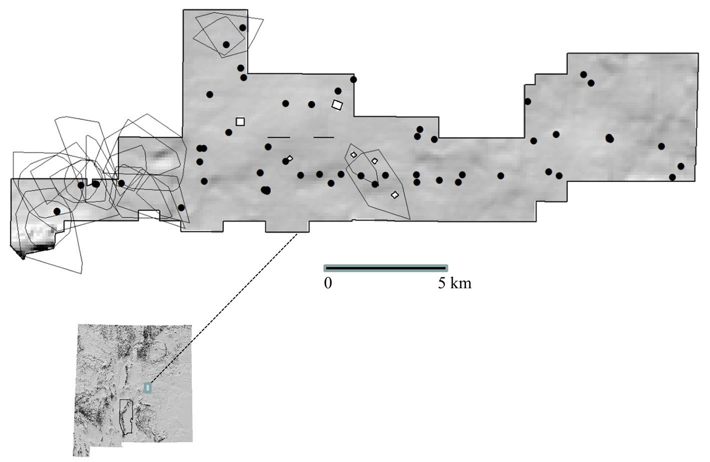
Figure 1. Topographic hillshade showing locations of annual home ranges of adult female mule deer (Bender et al., 2013), and locations of permanent water sources on the Corona Range and Livestock Research Center (CRLRC), east-central New
Mexico, USA.
We compared movement distances (km from continuous-time movement models [ctmms]; m between successive subdaily locations) between seasons using PROC GLIMMIX in SAS 9.4 (SAS, 1988), using individual deer as a random effect. We also compared mean daily and subdaily movements between successive seasons for individual deer for which we had both winter and subsequent spring-autumn data, or spring-autumn and subsequent winter data, available. We determined mean seasonal differences in movement distances for each successive time period for each individual, and used bootstrapping with N = 1,000 iterations to determine the probability that mean movement distances differed seasonally for this subset of data (see Efron & Tibshirani, 1993).
Additionally, because lactating females enter winter in poorer condition than do dry females and condition subsequently converges between the 2 classes over winter (including on the CRLRC; Bender & Hoenes, 2017), lactation status might affect desire or need to forage and thus movements of deer. However, because deer condition was very low on CRLRC during our study (i.e., lactating females were able to accrue only ≤ 5.7% percent body fat annually at the annual peak in late autumn; Bender et al., 2011, 2013), our GPS/VHF collared sample contained ≤ 2 lactating females each year, and thus we were unable to meaningfully include lactation status in our analyses. Consequently, we explored any potential effect of lactation status on movements by determining the percentile movement distances of lactating females relative to the frequency distribution of dry female movement distances to determine whether lactating females were closer to the mean or extremes of the range of dry females.
Lastly, because our GPS collared sample comprised a limited proportion of the overall radio-collared sample, we compared annual, spring-autumn, and winter home range sizes (Bender et al. 2013; N = 18-27 collared females annually) to see whether movements of our GPS sample were representative of radio-collared deer in general, comprised of N = 18-27 VHF-only collared adult females for each season (Bender et al., 2011, 2013). For this we compared annual and seasonal home range sizes of the 2 classes (GPS/VHF and VHF-only) using PROC GLM (SAS, 1988), specifically testing the year × class interaction. We visually located all deer (i.e., both GPS/VHF and VHF-only) via ground tracking of VHF signals a minimum of once per week with additional location emphasis on spring-autumn locations, and mapped locations using the Geographic Information System software package ArcGIS 10.0 (Environmental Systems Research Institute, Redlands, California, USA) (Bender et al., 2011, 2013). We constructed 95% minimum convex polygon (MCP) annual and seasonal home ranges after determining the minimum number of locations to adequately estimate seasonal home range size by plotting size as a function of number of locations (Bender et al. 2013; Kie et al. 1996). For this comparison we used only VHF visual locations of GPS/VHF collared deer so that both GPS/VHF and VHF-only samples were comprised of comparable data.
Results
We collected GPS movement data for 37 seasonal ranges (Table 2), winter 2005-6 through winter 2007-8, from 6-10 GPS/VHF collared adult females annually (mean = 336 and 472 locations per deer for winter and spring-autumn ranges, respectively). For all deer, the OUF-anisotropic movement model provided the best fit (i.e., AICc < 2 vs. all other models) of deer movements. The OUF-anisotropic movement model is the most general of ctmms, and includes a home range, correlated positions, correlated velocities, and movements varying by direction (Calabrese et al., 2021; Fleming et al., 2014).
Table 2
Mean distance moved by adult female mule deer during winter (Dec.-Feb.) and spring-autumn (Mar.-Nov.) seasons as estimated by continuous-time movement modeling (daily) and subdaily straight line movements between successive 4 h locations (subdaily) on the Corona Range and Livestock Research Center, east-central New Mexico, 2005-2007.
| Daily (km) | Subdaily (m) | |||||
| Season | Distance | SE | N | Distance | SE | N |
| Winter | 2.90 | 0.24 | 24 | 302 | 19 | 24 |
| Spring-Autumn | 4.34 | 0.43 | 13 | 409 | 44 | 13 |
Deer moved less during the winter (Table 2) for both daily ctmms (F1,20 = 6.0; p = 0.024) and minimum subdaily straight-line distances (F1,20 = 4.8; p = 0.041); in both cases the magnitude of differences varied among individual deer (t15 < -2.72; p < 0.016). Similarly, for deer for which movement data for successive seasons were available, movements between successive seasons were always less during the winter season (p (winter < spring-autumn) = 1.000) than the following or preceding spring-autumn season (Table 3).
Additionally, movement distances of lactating females (mean = 42nd percentile; range = 34-55th percentile) were always closer to the average than the extremes of the frequency distribution of movement distances of dry females for each period. Last, neither annual, spring-autumn, or winter home MCP range sizes (N = 7-16 per period) differed between GPS/VHF and VHF-only collared deer (F5,39 ≤ 0.94; p ≥ 0.599).
Discussion
Despite much less snow and warmer winter temperatures, mule deer females moved less during winter regardless of movement period (i.e., daily, subdaily), supporting the maintenance of this energy conservation behavior in mule deer in the arid Southwest (Verme & Ullrey, 1984). Because deep snow cover and very cold temperatures are typically lacking in the arid Southwest, our results further support low forage quality and availability being the primary drivers of this behavior in deer (Verme & Ullrey, 1984; see below). This latter was reflected by the poor nutritional condition of lactating adult females in the study area (i.e., <5.7% body fat annually at the annual peak in late autumn; Bender et al., 2011, 2013), and in the arid Southwest in general (Bender et al., 2007, 2011, 2012; Bender, 2020), as well as the significant losses in condition seen over winter (Bender & Hoenes, 2017; Hoenes, 2008), despite mule deer likely requiring lower quality forage than white-tailed deer (O. virginianus) (Staudenmaier et al., 2022).
While lack of deep snow cover may result in relative forage availability being less impacted during winter in the arid Southwest, senesced forages are still of very low quality, similar to northern environments (Kemp, 1983; Krausman et al., 1990; McKinney, 2003). Low forage quality in winter was reflected in the condition dynamics of deer on the CRLRC; for example, dry females lost on average 32% of body fat reserves and 38% of rump body condition score over winter (L. Bender, unpublished data), even though their condition in late autumn-early winter was already low relative to other southwestern populations (Bender et al., 2007, 2011, 2012). The nutritional condition of deer is driven primarily by forage quality (Bender, 2020; National Research Council, 2007; Tollefson et al., 2010; Verme & Ullrey, 1984; Wakeling & Bender, 2003), illustrating that deer in the arid Southwest face similar constraints in terms of limited nutrient gains from forage intake as do deer in northern environments during winter.
Table 3
Mean movement distances (x) and mean differences (D) in mean distance moved daily as predicted by continuous-time movement modeling (daily) and subdaily straight line movements between successive 4 h locations (subdaily) of adult female mule deer for which movement data for successive seasons were available between winter (Dec.-Feb.) and spring-autumn (Mar.-Nov.) on the Corona Range and Livestock Research Center, east-central New Mexico, 2005-2007. p = Probability that seasonal differences differ from 0; N = number of seasonal comparisons.
| Period | x Summer | x Winter | D | 90% CI | p | N |
| Subdaily | 400.2 | 309.6 | -90.6 m | -123- -63 | 1.000 | 20 |
| Daily | 4.21 | 3.16 | -1.05 km | -1.53- -0.63 | 1.000 | 20 |
Deer in northern environments do face additional energetic challenges associated with persistent snow cover, which can limit forage availability (by making location and acquisition of food more difficult; Hovey & Harstad, 1992), diet quality (due to reduced forage quality and availability; McKinney, 2003; Osborn & Jenks, 1998), and increase loss of endogenous reserves (because of increased costs of moving through snow; Bunnell et al., 1990; Mattfeld, 1973). However, while deer in the arid Southwest are less influenced by snow-depth related challenges, northern deer do not face the lack of free water experienced by most deer populations in arid environments because of persistent snow cover in northern environments. Lack of water can present an energetic cost to deer in the arid Southwest, as mule deer may increase movement distances to access water (Heffelfinger, 2006), and winter is much drier than spring-autumn in Chihuahuan desert and short-grass prairie habitats of the arid Southwest (e.g., 87% of precipitation occurs during spring-autumn on the CRLRC).
Because of permanent water developments, water was comparably available seasonally on the CRLRC; water developments were accessible from all deer home ranges, so mule deer did not need to alter their movements in response to seasonal changes in availability of water. Hence, need or preference for free water likely had a negligible effect on deer movements on the CRLRC, unless presence of temporary sources (ephemeral pools, etc.) during the summer monsoon reduce deer movements during spring-autumn because of increased availability. Thus, despite water being effectively controlled in our study, deer still showed less movements during winter. This again supports decreased movements during winter being most influenced by the lack of energetic benefit from seeking and foraging on low quality senesced forage.
Cold temperatures are often thought to influence the winter conservation strategy, despite demonstrated lack of benefit of thermal cover in winter to deer (Cook et al., 1998; Freddy, 1984), the pronounced effect of solar radiation on warming deer (Cook et al., 1998; Parker & Gillingham, 1990; Parker & Robbins, 1984), and deer movements and tolerance of exposure to cold (including bedding in the open) except during the most extreme conditions when high quality forage is available (Moen, 1968; Verme & Ullrey, 1984). Mule deer possess a low thermal critical zone (ca. -20 oC) and show greater tolerance of cold than do white-tailed deer, including a lower metabolic rate response to decreasing temperatures (Mautz et al., 1985; Parker & Robbins, 1984). Hence, they are less affected by even extreme cold, which is seldom the case in the arid Southwest where mean low temperatures seldom approach their lower thermal tolerance (Table 1). Conversely, the upper thermal critical level of mule deer in winter pelage (5 ºC; Mautz et al., 1985) is lower than average high temperatures during winter on our study area (6.7-8.9 ºC; Table 1) and much of the arid Southwest. This would require active metabolic activity or behaviors (e.g., panting, etc.) by mule deer to cool themselves, or possibly limiting movements and bedding under shade (although the energetic benefits of the latter are questionable; Cook et al., 1998). Consequently, if temperature affected movements during the winter in our study area, deer would be more likely to decrease movements because of heat stress, not cold stress.
Lastly, while at least one behavioral aspect of the winter energy conservation strategy is seen in mule deer in the arid Southwest, to what degree other adaptations are conserved is unknown. Mule deer in the arid Southwest do develop a highly insulative pelage in winter (Heffelfinger, 2006), but the extent that they may decrease metabolic rate or regulate vascular circulation to the extremities (or need to, in light of the more moderate temperatures) is unknown. Additionally, while lactating females showed a tendency to move less relative to dry females on the CRLRC, whether this is typical is unknown because of our small sample of lactating females. However, given that most females on CRLRC were in poorer condition than females elsewhere in the arid Southwest (Bender et al., 2007, 2011, 2012; Bender & Hoenes, 2017), if very low condition (such as results from lactation) increases movements during winter, this increase would likely have been seen in all CRLRC females regardless of lactation status. Moreover, GPS/VHF and VHF-only collared females showed similar movements (as indexed by home range sizes) seasonally and annually on CRLRC, indicating that movements of GPS/VHF collared females reflected females in general. Although small sample sizes (3-4) precluded including lactation status as an interactive term in the contrast of GPS/VHF and VHF-only collared females, for all females lactation status had no effect on annual or seasonal home range sizes (p ≥ 0.599).
Acknowledgments
Support for this project was provided by the U.S. Forest Service-Rocky Mountain Research Station and the New Mexico State University Cooperative Extension Service and Agricultural Experimental Station. All activities were in accordance with NMSU IACUC Permit No. 2005-023. E.J.T.-R. was supported by a postdoctoral fellowship from Consejo Nacional de Humanidades, Ciencias y Tecnologías (Conahcyt-Mexico).
References
Alldredge, A. W., Lipscomb, J.F., & Whicker, F.W. (1974). Forage intake rates of mule deer estimated with fallout
cesium-137. The Journal of Wildlife Management, 38, 508–516. https://doi.org/10.2307/3800882
Bartmann, R. M., & Bowden, D. C. (1984). Predicting mule deer mortality from weather data in Colorado. Wildlife Society Bulletin, 12, 246–248. https://doi.org/10.1002/jwmg.956
Bender, L. C. (2020). Elk, deer, and pinyon-juniper: needs, what works, and what doesn’t. In K. Malcolm, B. Dykstra, K. Johnson, D. Lightfoot, E. Muldavin, & M. Ramsey (Compilers), Symposium proceedings on piñon-juniper habitats: status and management for wildlife – 2016. Proceedings RMRS-P-77. Fort Collins, Colorado: U.S. Forest Service, Rocky Mountain Research Station.
Bender, L. C., & Hoenes, B. D. (2017). Costs of lactation to body condition and future reproduction of free-ranging mule deer Odocoileus hemionus (Cervidae). Mammalia, 81, 329–338. https://doi.org/10.1515/mammalia-2015-0143
Bender, L. C., Lomas, L. A., & Browning, J. (2007). Condition, survival, and cause-specific mortality of mule deer in northcentral New Mexico. Journal of Wildlife Management, 71, 1118–1124. https://doi.org/10.2193/2006-226
Bender, L. C., Boren, J. C., Halbritter, H., & Cox, S. (2011). Condition, survival, and productivity of mule deer in semiarid grassland-woodland in east-central New Mexico. Human-Wildlife Interactions, 5, 276–286. https://doi.org/10.26077/60n0-ks48
Bender, L. C., Hoenes, B. D., & Rodden, C. L. (2012). Factors influencing survival of desert mule deer in the greater San Andres Mountains, New Mexico. Human-Wildlife Interactions, 6, 245–260. https://doi.org/10.26077/h5bg-1829
Bender, L. C., Boren, J. C., Halbritter, H., & Cox, S. (2013). Effects of site characteristics, pinyon-juniper control, and precipitation on habitat quality for mule deer on the Corona Range and Livestock Research Center. Human-Wildlife Interactions, 7, 47–59. https://digitalcommons.usu.edu/hwi/vol7/iss1/5
Bunnell, F. L., Hovey, F. W., McNay, R. S., & Parker, K. L. (1990). Forest cover, snow conditions, and black-tailed deer sinking depths. Canadian Journal of Zoology, 68, 2403–2408. https://doi.org/10.1139/z90-333
Calabrese, J. M., Fleming, C. H., & Gurarie, E. (2016). ctmm: an R package for analyzing animal relocation data as a continuous-time stochastic process. Methods in Ecology and Evolution, 7, 1124–1132. https://doi.org/10.1111/2041-210X.12559
Calabrese, J. M., Fleming, C. H., Noonan, M. J., & Dong, X. (2021). ctmmweb: a graphical user interface for autocorrelation-informed home range estimation. Wildlife Society Bulletin, 45, 162–169. https://doi.org/10.1002/wsb.1154
Cook, J. G., Irwin, L. L., Bryant, L. D., Riggs, R. A., & Thomas, J. W. (1998). Relations of forest cover and condition of elk: a test of the thermal cover hypothesis in summer and winter. Wildlife Monographs, 141, 1–61.
Efron, B., & Tibshirani, R. J. (1993). An introduction to the bootstrap. New York: Chapman & Hall.
Fleming, C. H., Fagan, W. F., Mueller, T., Olson, K. A., Leimgruber, P., & Calabrese, J. M. (2014). From fine-scale foraging to home ranges: a semivariance approach to identifying movement modes across spatiotemporal scales. American Naturalist, 183, E154–E167. http://doi.org/10.1086/675504
Fleming, C. H., Fagan, W. F., Mueller, T., Olson, K. A., Leimgruber, P., & Calabrese, J. M. (2016). Estimating where and how animals travel: an optimal framework for path reconstruction from autocorrelated tracking data. Ecology, 97, 576–582. https://doi.org/10.1890/15-1607.1
Freddy, D. J. (1984). Quantifying capacity of winter ranges to support deer – evaluation of thermal cover used by deer. Denver, CO: Wildlife Research Report, Colorado Division of Wildlife, USA.
Heffelfinger, J. (2006). Deer of the Southwest: a complete guide to the natural history, biology, and management of Southwestern mule deer and white-tailed deer. Texas A&M University, College Station, Texas.
Hoenes, B. D. (2008). Identification of factors limiting desert mule deer populations in the greater San Andres Mountains of southcentral New Mexico (Thesis). New Mexico State University, Las Cruces.
Hovey, F. W., & Harestad, A. S. (1992). Estimating effects of snow on shrub availability for black-tailed deer in southwestern British Columbia. Wildlife Society Bulletin, 20, 308–313.
Jacobsen, N. K. (1980). Differences of thermal properties of white-tailed deer pelage between seasons and body regions. Journal of Thermal Biology, 5, 151–158. https://doi.org/10.1016/0306-4565(80)90014-5
Kemp, P. R. (1983). Phenological patterns of Chihuahuan desert plants in relation to the timing of water availability. Journal of Ecology, 71, 427–436.
Kie, J. G., Baldwin, J. A., & Evans, C. J. (1996). CALHOME: a program for estimating animal home ranges. Wildlife Society Bulletin, 24, 342–344.
Krausman, P. R., Ordway, L. L., Whiting, F. M., & Brown, W. H. (1990). Nutritional composition of desert mule deer forage in the Picacho Mountains, Arizona. Desert Plants, 10, 32–34.
Marchinton, R. L., & Hirth, D. H. (1984). Behavior. In L. K. Halls (Ed.), White-tailed deer ecology and management. Pennsylvania: Stackpole Books.
Marshal, J. P., Krausman, P. R., & Bleich, V. C. (2008). Body condition of mule deer in the Sonoran Desert is related to rainfall. Southwestern Naturalist, 53, 311–318. https://doi.org/10.1894/CJ-143.1
Mattfeld, G. F. (1973). The effect of snow on the energy expenditure of walking white-tailed deer. In Transactions of the 30th Northeast Fish and Wildlife Conference, Dover, Vermont, Spring, April 1973.
Mautz, W. W., Pekins, P. J., & Warren, J. A. (1985). Cold temperature effects on metabolic rates of white-tailed, mule, and black-tailed deer in winter coat. In P. F. Fennessy, & K. R. Orew (Eds.), The biology of deer. Royal Society of New Zealand Bulletin, 22, 453–457.
McKinney, T. (2003). Precipitation, weather, and mule deer. In J. C. Jr. deVos, M. R. Conover, & N. E. Headrick (Eds.), Mule deer conservation. Issues and management strategies. Logan, Utah: Jack H. Berryman Press.
Moen, A. N. (1968). Energy exchange of white-tailed deer, western Minnesota. Ecology, 49, 676–682. https://doi.org/10.2307/1935531
National Research Council (US). (2007). Committee on Nutrient Requirements of Small Ruminants. Nutrient requirements of small ruminants: sheep, goats, cervids, and New World camelids. Washington D.C.: National Academy Press.
Osborn, R. G., & Jenks, J. A. (1998). Assessing dietary quality of white-tailed deer using fecal indices: effects of supplemental feeding and area. Journal of Mammalogy, 79, 437–447. https://doi.org/10.2307/1382974
Parker, K. L., & Robbins, C. T. (1984). Thermoregulation in mule deer and elk. Canadian Journal of Zoology, 62, 1409–1422. https://doi.org/10.1139/z84-202
Parker, K. L., & Gillingham, M. P. (1990). Estimates of critical thermal environments for mule deer. Journal of Range Management, 43, 73–81. http://doi.org/10.2307/3899126
Robinette, W. L., Jones, D. A., Rogers, G., & Gashwiler, J. S. (1957). Notes on tooth development and wear for Rocky Mountain mule deer. Journal of Wildlife Management, 21, 134–153. https://doi.org/10.2307/3797579
SAS. (1988). SAS/STAT user’s guide. SAS Institute Incorporated, Cary, North Carolina.
Short, H. L. (1981). Nutrition and metabolism. In O. C. Wallmo, R. E. McCabe, & L. R. Jahn (Eds.), Mule and black-tailed deer of North America. Lincoln: University of Nebraska Press.
Silver, H., Holter, J. B., Colovox, N. F., & Hayes, H. H. (1971). Effect of falling temperature on heat production in fasting white-tailed deer. Journal of Wildlife Management, 35, 37–46.
Staudenmaier, A. R., Shipley, L. A., Camp, M. J., Forbey, J. S., Hagerman, A. E., Brandt, A. E. et al. (2022). Mule deer do more with less: comparing their nutritional requirements and tolerances with white-tailed deer. Journal of Mammalogy, 103, 178–195. https://doi.org/10.1093/jmammal/gyab116
Tollefson, T. N., Shipley, L. A., Myers, W. L., Keisler, D. H., & Dasgupta, N. (2010). Influence of summer-autumn nutrition on body condition and reproduction in lactating mule deer. Journal of Wildlife Management, 74, 974–986. https://doi.org/10.2193/2008-529
Verme, L. J., & Ullrey, D. E. (1984). Physiology and nutrition. In L. K. Halls (Ed.), White-tailed deer: Ecology and management. Harrisburg, Pennsylvania: Stackpole Books.
Wakeling, B. F., & Bender, L. C. (2003). Influence of nutrition on mule deer biology and ecology. In J. C. Jr. deVos, M. R. Conover, & N. E. Headrick (Eds.), Mule deer conservation. Issues and management strategies. Logan, Utah: Jack H. Berryman Press.

Impacts of disturbance on ant (Hymenoptera:Formicidae) food preferences and dominance in a Mexican temperate forest.
Meghan I. Zolá-Rodríguez a, Mariana Cuautle b, *, Marco Daniel Rodríguez-Flores c, Citlalli Castillo-Guevara b
a Akumal Monkey Sanctuary & Rescued Animals, Camino a Uxuxubi s/n Predio Santa Pilar Lote 16, 77776 Akumal, Quintana Roo, Mexico
b Universidad Autónoma de Tlaxcala, Centro de Investigación en Ciencias Biológicas, Km 10.5 Carretera Tlaxcala-San Martín Texmelucan, 90120 San Felipe Ixtacuixtla, Tlaxcala, Mexico
c Blue Marlin Conservation (Conservation Diver), Sunset Beach Gili Air, Gili Indah, Pemenang, North Lombok Regency, West Nusa Tenggara 83355, Indonesia
*Corresponding author: mcuautle2004@gmail.com (M. Cuautle)
Received: 26 June 2024; accepted: 27 August 2024
Abstract
This study examines the impact of disturbance on the food preferences and dominance of an ant community in a temperate ecosystem in Mexico. The study focused on 2 types of vegetation: native oak forest and induced grassland (disturbed vegetation). Observations were conducted to record the food elements carried by ants to their nests. These data were analyzed using x2 tests. Tuna and honey baits were placed near the nests to record the presence of ants in 5-minute periods. We used a binomial model to determine whether the probability of finding an ant foraging at the baits was affected by vegetation type, bait type, and/or ant species. Additional baits were used to determine the ant dominance indices. T-tests and ANOVAs were used to compare dominance indices between vegetation types, baits, and ant species. No significant differences were observed in food preferences between vegetations. However, some species showed a preference for honey (i.e., carbohydrates), which could be limited in ground-level environments. Ants showed a submissive behavior in both vegetation types. This research shows that ants could optimize their nutrient intake, enabling them to survive efficiently even when facing disturbances, instead of increasing dominance.
Keywords: Ant nest; Dominance index; Feeding habits; Compensation hypothesis; Carbohydrates; Proteins
© 2024 Universidad Nacional Autónoma de México, Instituto de Biología. Este es un artículo Open Access bajo la licencia CC BY-NC-ND
(http://creativecommons.org/licenses/by-nc-nd/4.0/).
Impacto del disturbio en las preferencias alimentarias y dominancia de las hormigas (Hymenoptera: Formicidae) en un bosque templado de México
Resumen
Este estudio examina el impacto del disturbio en las preferencias alimentarias y dominancia de una comunidad de hormigas en un ecosistema templado en México, en bosque de encino nativo y pastizal inducido (vegetación perturbada). Se registraron los alimentos transportados por las hormigas a sus nidos. Estos datos fueron analizados utilizando pruebas de x2. Se colocaron cebos de atún y miel cerca de los nidos para registrar la presencia de hormigas. Utilizamos un modelo binomial para determinar si la probabilidad de encontrar una hormiga en los cebos se veía afectada por la vegetación, cebo o especie de hormiga. Los índices de dominancia se determinaron usando cebos. Se emplearon pruebas t y Anova para comparar los índices de dominancia entre tipos de vegetación, cebos y especies de hormigas. No hubo diferencias significativas en las preferencias alimentarias entre tipos de vegetación, pero algunas especies mostraron una preferencia por la miel (carbohidratos), que podría ser un recurso limitado a nivel del suelo. Las hormigas mostraron un comportamiento sumiso en ambos tipos de vegetación. Esta investigación muestra que las hormigas podrían optimizar su ingesta de nutrientes, permitiéndoles sobrevivir bajo condiciones de disturbio, en lugar de aumentar su dominancia.
Palabras clave:Nidos de hormigas; Índice de dominancia; Hábitos alimenticios; Hipótesis de compensación; Carbohidratos; Proteínas
Introduction
Land use change stands as one of the primary factors contributing to global change and its adverse effects on biodiversity (Ellis et al., 2010; Foley et al., 2005; Sala et al., 2000). Land use change has reduced biodiversity through the loss, modification, and fragmentation of habitats; degradation of soil and water; and overexploitation of native species (Foley et al., 2005), and its effects depend strongly on the type, severity, frequency and timing of disturbance (Foley et al., 2005; White & Jentsch, 2001). Ants are one of the most dominant insects both ecologically and numerically (Rico-Gray & Oliveira, 2007; Schultheiss et al., 2022; Toro et al., 2012) that participate in different ecological processes —e.g., nutrient recycling, soil formation, decomposition, seed dispersion (Toro et al., 2012). Ants are model organisms to study the effect of disturbance because they respond to environmental change (Agosti et al., 2000; Andersen, 2000). It is often observed that disturbances favor behaviorally dominant ants, including invasive species. Vonshak and Gordon (2015), observed that native ant richness was highest in natural habitats, and alien species richness was highest in urban habitats, along an urban-rural gradient in the San Francisco Bay area. Nevertheless, the specific effect will depend on factors like the type of disturbance, including fires, floodings, or even treefall gaps (Cerdá et al., 2013). Hoffman and Andersen (2003) studied the response of ant functional groups to disturbance finding that the dominant Dolichoderinae and “hot climate specialists” tend to be favoured by low levels of disturbance. The opportunist and generalized Myrmicinae have wide habitat tolerances but are sensitive to competitive interactions, while “cryptic species” and “specialist predators” are highly sensitive to disturbance.
Feeding habits and foraging strategies represent vital life history traits among ants, playing a significant role in their ecological dynamics. These traits are contingent upon the availability of resources within their respective habitats (Andersen, 2000; Davidson, 2005), and the ensuing competition for those resources (Arnan et al., 2012). The feeding habits of ants play a pivotal role in determining their ecological function within the ecosystem (Spotti et al., 2015). However, despite their significance, the food habits and preferences of ants remain relatively understudied and represent one of the least understood aspects of their biology (Houdria et al., 2015).
The effects of disturbance (e.g., land use change) on ant feeding habits (especially foraging strategies) have not been studied in depth (Castillo-Guevara et al., 2019; Hernández-Flores et al., 2016; Radnan et al., 2018), and the way ants respond to habitat complexity can provide clues as to how ants could respond to disturbance. When the external disturbing factors are of high intensity (natural-fires or anthropogenic-deforestation), the disturbances can initiate a directional regression manifested as gradual or rapid simplification of the horizontal and vertical structure of a community, leading to the replacement of complex communities by a simpler one (Łaska, 2001). The level of habitat complexity can influence ant foraging patterns. For instance, higher complexity may decrease interspecific interactions and ant recruitment or minimize the trade-off between resource discovery and dominance (Parr & Gibb, 2012).
Examining the effect of soil surface complexity on food exploitation in the context of change from grassland to shrubland in Australia, Radnan et al. (2018) discovered that substrate complexity (wood debris, leaf litter, or no substrate) influenced the discovery time, ant size, and monopolization index of tuna and honey baits within testing arenas. However, at a larger scale of vegetation type, the effect was not observed. Similarly, Castillo-Guevara et al. (2019) found that the dominance level was similar in natural oak vegetation in comparison to an agricultural area in a temperate community; however, ant foraging strategies differed between the 2 communities.
Competition has been regarded as the primary factor influencing the structure of ant communities (Cerdá et al., 2013). Through the use of aggressive strategies, ants exert influence on the spatial distribution, abundance, and behavior of other ants. These strategies encompass a range of tactics, including the deployment of repellent chemicals and the establishment of territories (Cerdá et al., 2013). Moreover, ants can establish interspecific dominance hierarchies primarily based on variations in food collection behavior and aggressiveness. While there are various proposals for categorizing such hierarchies, the classification proposed by Vepsäläinen and Pisarski (1982) and Savolainen et al. (1989), as described by Cerdá et al. (2013), is considered the most well-defined hierarchical system from an ecological perspective. This classification system is founded on the aggressive behavior of ants and its impact on other ant species, and includes 3 categories: the dominant, subdominant and subordinate category. Dominant species exhibit highly aggressive behavior, exhibit numerical predominance over other species, fiercely defend their territories, and establish mutual exclusivity within their ecological communities. Subdominant species, while not actively defending territories, display a remarkable propensity for aggressively safeguarding their food resources (Cerdá et al., 2013). Lastly, subordinate species, characterized by small colonies devoid of recruitment systems, employ strategies to avoid physical confrontations with other colonies and species. Nonetheless, they exhibit a strong commitment to defending their nests against potential threats (Cerdá et al., 2013). Different foraging strategies, such as the subordinate species’ ability to discover resources before dominant species (dominance-discovery trade-off, Fellers, 1987) or their capacity to forage across a broader temperature range compared to dominant species —dominance-thermal tolerance trade-off (Fellers, 1989), can contribute to the coexistence of ants within a community.
The present study focuses on the analysis of ant feeding habits and dominance hierarchy in response to land use change within a temperate ecosystem located in central Mexico. A habitat with the native oak forest vegetation (complex habitat), was compared to a nearby area where the land use had been altered to induced grassland (simplified habitat). The study hypothesized: i) it is expected that in the oak forest, food items transported to the nest will be more varied than in the induced grassland. This variation at the species level is also anticipated due to the change in land use. The conversion from a complex habitat (oak forest) to a simplified habitat (induced grassland) will likely provide fewer resources variety for the ants; ii) it is expected that as a result of the disturbance in the induced grassland, ants will be more generalized in low heterogeneous habitats due to the dominance of generalist ant species. Additionally, the arrival times at the baits will be shorter due to the absence of leaf litter; iii) a lower dominance index is expected in the induced grassland than in the oak forest, due to the presence of subdominant species and the modification of the dominance hierarchy system by the land use change.
Materials and methods
The study was conducted within “Flor del Bosque” State Park, located in the municipality of Amozoc de Mota, in the state of Puebla. The coordinates of this protected reserve are 19°00’00”-19°01’50” N, 98°20’35”-98°20’53” W. The State Park encompasses an area of 664.03 hectares, characterized by altitudes ranging from 2,225 to 2,400 m asl. The annual average temperature in this region fluctuates between 14 °C and 16 °C, with the majority of rainfall occurring during the summer months, contributing to an average annual precipitation of 750 to 950 mm. It is important to note that the park experiences a distinct dry season lasting approximately 6 months, from November to April, as reported by Costes et al. (2006). The native vegetation of the reserve primarily consists of oak forest [Quercus castanea (Née), Q. laurina (Bonpl.), Q. laeta (Liebm.) (Fagaceae)]. However, human disturbances have led to the presence of induced grassland areas and, to a lesser extent, eucalyptus plantations [Eucalyptus spp. L´Hér) (Myrtaceae)] within the park, as documented by Costes et al. (2006). Given that the disturbed vegetation within the reserve primarily consisted of induced grassland, our research aimed to establish a meaningful comparison between native and altered vegetation.
Ant communities were surveyed once a month during specific periods (April, August and October 2015, and January to March 2016). The survey methodology involved the establishment of 6 transect plots (400 m × 20 m), with 3 plots located in the oak forest and 3 in the induced grassland. The spatial distribution of these transects can be observed in Figure 1. To locate ant nests, the transects were traversed, and various substrates such as leaf litter, stones, trunks, and branches were lifted and examined. Additionally, a total of 5 tuna baits and 5 honey baits were placed along the transects at 10 m intervals to attract ants and to follow them to locate their nest. The nests found during the survey were georeferenced for accurate spatial documentation. A 5-minute observation period was designated for each nest, wherein all food items transported by the ants to their nests were recorded. These observations were conducted between 9:00 a.m. and 3:00 p.m. on the sampling days. Each recorded item was subsequently categorized into one of the following groups: 1) plant elements, encompassing any component of plants except for seeds, 2) seeds, and 3) arthropods. After each observation period, 2 bait samples, enclosed within Petri dishes, were positioned in close proximity to the nests (approximately 10 cm), maintaining a distance of approximately 5 centimeters from each other. Various studies exploring the feeding habits, preferences, and foraging strategies of ants have employed diverse bait types. Typically, these baits consist of carbohydrates such as honey and other sources representing proteins such as tuna (Houdria et al., 2015; Lynch et al., 1980; Spotti et al., 2015; Trigos-Peral et al., 2016). The bait materials employed in the study consisted of honey and tuna, which were consistently provided in a standardized amount of one tablespoon, equivalent to approximately 5 grams. To quantify the number of individual ants on each type of food resource, we placed baits and observed them for 5 min. Ants responded very quickly to the baits; therefore, the observation time was limited to 5 min. Within this duration, the number of individuals was recorded for each bait type. After the observation periods, 1 to 3 ants were collected from each nest using a vacuum cleaner or tweezers and then preserved in Eppendorf tubes containing 70% ethanol. In the laboratory, the ants were separated, mounted, and identified to the genus level using the key by Mackay and Mackay (1989). In certain instances, the species identification was feasible by comparing the collected specimens with those present in the Entomological Collection of the Universidad de las Américas Puebla (UDLAP).
To analyze the food preferences of the ant community, we considered 3 factors. First, we determined whether the number of foragers carrying plants, seeds, or arthropods to the nest differed between the whole ant communities of each vegetation type or among ant species. We used the appropriate contingency tables and chi-square tests for such comparisons. Second, we determined whether the presence of foragers at each bait during each minute of the 5-minute period was influenced by vegetation type, bait type (honey or tuna), ant species or interactions among these factors. We used a binomial model to evaluate this response variable, with “ant presence” coded as 1 and “absence” as 0. To select the most relevant explanatory variables, we employed a stepwise forward approach. We began with the simplest model and successively added each response variable. The significance of adding each variable was assessed using an x2 test, comparing the previous model with the new model. If a variable was found to be statistically significant, it was retained in the model. Otherwise, it was removed, and we proceeded with the next explanatory variable. This stepwise procedure allowed us to build the final model with the most significant factors explaining the presence of foragers at each bait. No overdispersion was detected in the selected model. Post-hoc analyses were conducted when significant differences were detected. The statistical analysis of data was performed using R software (R Core Team, 2022).
We evaluated the dominance hierarchy of the ants in each vegetation type (oak forest and induced grassland), ant species, and bait types using the same transects as for the detection of the nests (Fig. 1), during October 2015 and January, February and March (2016). At each transect, 9 sampling points were established on the ground, spaced 10 m apart. Each sampling point consisted of a pair of Petri dishes with baits: one with honey and one with tuna, placed less than 5 cm apart. This resulted in a total of 540 baits (5 replicates × 6 transects × 9 sampling points × 2 baits; 2 samplings in February). These types of baits have been widely used for ant dominance hierarchy studies (Dáttilo et al., 2014; Parr & Gibb, 2012; Trigos-Peral et al., 2016).
For the first 3 sets of bait, we recorded the arrival times of the ants during a one-hour observation period. Most of the ant species were identified in the field. For the ants that were not identified, a few individuals (2 to 3 specimens) were collected. In the case of the remaining 6 sets of bait, they were filled with water. Ants that fell onto the Petri dish after 2 h were collected. The presence of water did not deter the ants from visiting, but it allowed us to determine which ants had been attracted to the baits. The baits were placed and retrieved from different transects in the field between 9:00 a.m. and 5:00 p.m. The order of the transects was changed on different sampling days to mitigate the potential impact of the time of day. Ant specimens collected from the baits were preserved in 70% ethanol and transported to the laboratory for further identification.

Figure 1. Localization of the transects used in the study zone (mapped by Luna F.).
We chose numerical dominance to assess the dominance hierarchy of the ants —i.e., ordering of ant species based on their numerical or behavioral dominance by vegetation types (Andersen, 1992; Cerdá et al., 1997; Stuble et al., 2017), ant species and bait type. As numerical and behavioral dominance are highly correlated, this method has been well-established and documented in the ant literature (Dáttilo et al., 2014; Dejean & Corbara, 2003; Parr, 2008; Parr & Gibb, 2012; Santini et al., 2007). This method indicates which species are consistently present at the baits, and which ones dominate the baits numerically and thus monopolize them (Parr, 2008). We represented numerical dominance using the numerical dominance index (DI) for each morphospecies calculated by the formula: DI = (Di)/(Di + Si), where, Di is the number of baits monopolized by the species of ant i, and Si is the number of baits that the species of ant i used but did not monopolize. Baits were considered to be monopolized when more than 5 individuals (workers and/or soldiers) of the same morphospecies were using the resource without the presence of other morphospecies. This measure (more than 5 individuals) takes into consideration that in temperate climates, ants are less abundant, and recruitment is considered weaker than in tropical environments where the index has been widely more (Santini et al., 2007). Therefore, dominant morphospecies are those that find and monopolize a larger proportion of the food resources in a given environment. The value of the index ranges from 0 (completely submissive species) to 1 (totally dominant species) and is similar to the “monopolization index” used in other studies (Dáttilo et al., 2014; Fellers, 1987; Parr & Gibb, 2012; Santini, et al., 2007). In this study, ant species with a DI lower than 0.5 were classified as submissive.
The arrival times of the ants were compared using survival curves using the survival package of the R Software program. The one-hour and 2-hour baits were used to calculate the ID of the ant species. To compare the ID between vegetation and bait types, t-tests were performed. To compare the DI between ant species, a one-way ANOVA test was performed after applying a square root transformation to meet the normality requirements. These analyses were performed using the program STATVIEW 5.0 (Abacus Concepts Inc., 1996).
Results
Fourteen morphospecies of ants were recorded in this study belonging to 11 ant genera (Table 1). For the analysis of the results from the nests and the baits placed near them, 2 morphospecies of Pheidole were identified. However, due to the low number of records for each morphospecies across different vegetation types, Pheidole sp. 1 and Pheidole sp. 2 were combined for the analysis. In the oak forest, 2 out of 19 records corresponded to Pheidole sp. 1, and in the grassland, 4 out of 15 records corresponded to Pheidole sp. 2. Since Pheidole species often share similar feeding habits and are functionally similar (Agosti, 2000; Andersen, 2000), these 2 morphospecies were grouped to increase statistical power, and the analysis was conducted at the genus level. In contrast, another Pheidole species, Pheidole sp. 3, was recorded in the baits used to determine the DI and was analyzed independently due to its different context of occurrence. The rest of the analyses were conducted at the species level.
In the case of the nests, we found 9 morphospecies distributed among 34 nests, 19 of these were located in the oak forest and 18 in the induced grassland (Table 2). No significant differences were observed in the types of food elements those individual ants transported to their nest when comparing different vegetation types (x2 = 2.13, df = 2, p = 0.34). In the oak forest considering all ant species, there were no significant differences in the number of individuals carrying elements from different categories (x2 = 0.03, df = 1, p = 0.86) (Fig. 2). Of the genera of ants observed carrying food elements to their nests, only 2 genera were observed with a single type of food resource: Prenolepis imparis (Say) only carried arthropods and Dorymyrmex insanus (Buckley) only seeds.
Table 1
List of ant species recorded in this study in “Flor del Bosque” State Park in Puebla, Mexico.
| Formicidae/Subfamily/Ant species | |||
| Formicidae Latreille, 1809 | |||
| Dolichoderinae Forel, 1878 | |||
| Leptomyrmecini Emery, 1913 | |||
| Dorymyrmex Mayr, 1866 | |||
| Dorymyrmex insanus (Buckley, 1866) | |||
| Linepithema Mayr, 1866 | |||
| Linepithema dispertitum (Forel, 1885) | |||
| Dorylinae Leach, 1815 | |||
| Dorylini Ashmead, 1905 | |||
| Labidus Jurine, 1807 | |||
| Labidus coecus Latreille, 1802 | |||
| Formicinae Latreille, 1809 | |||
| Camponotini Forel, 1878 | |||
| Camponotus Mayr,1861 | |||
| Camponotus rubrithorax Forel, 1899 | |||
| Lasiini Ashmead, 1905 | |||
| Nylanderia Emery, 1906 | |||
| Nylanderia austroccidua Trager, 1984 | |||
| Prenolepis Mayr, 1861 | |||
| Prenolepis imparis Say, 1836 | |||
| Myrmicinae Lepeletier, 1835 | |||
| Attini Smith, 1858 | |||
| Pheidole Westwood, 1839 | |||
| Pheidole sp. 1 | |||
| Pheidole sp. 2 | |||
| Pheidole sp. 3 | |||
| Crematogastrini Forel, 1893 | |||
| Temnothorax Mayr, 1861 | |||
| Temnothorax augusti Baroni Urbani, 1978 | |||
| Pogonomyrmecini Ward, Brady, Fisher & Schultz, 2014 | |||
| Pogonomyrmex Mayr, 1868 | |||
| Pogonomyrmex barbatus (Smith, F., 1858) | |||
| Solenopsidini Forel, 1893 | |||
| Monomorium Mayr, 1855 | |||
| Monomorium ebenium Forel, 1891 | |||
| Pseudomyrmecinae, Smith, M.R., 1952 | |||
| Pseudomyrmecini Smith, 1952 | |||
| Pseudomyrmex Lund, 1831 | |||
| Pseudomyrmex pallidus Smith, F., 1855 |
Conversely, ants of the genus Pheidole spp. carried a greater quantity of plant elements compared to the other categories (x2 = 10.4, df = 2, p = 0.006); only 2 of these individuals were observed carrying arthropods, and none were recorded carrying seeds. No significant differences were found for D. insanus (x2 = 2, df = 2, p = 0.37), P. barbatus (x2 = 1.6, df = 2, p = 0.450), nor P. imparis (x2 = 4, df = 2, p = 0.135) among the 3 food categories. Only P. barbatus carried all 3 types of food (Fig. 2).
Considering all ant species, there were no significant differences in the number of individuals carrying different food elements in the induced grassland (x2 = 0.66, df = 1, p = 0.41, Fig. 2). Among the observed ant species that transported food types to their nests, P. barbatus was found to carry both plant elements and seeds. Additionally, Dorymyrmex insanus and Pheidole spp. were observed carrying food from all 3 categories (Fig. 2). Pheidole spp. (x2 = 10.33, df = 2, p = 0.006) and P. barbatus (x2 < 30.33, df = 2, p < 0.001), carried a higher number of plant elements. For D. insanus no significant differences were found in the number of elements of each type (x2 < 3.77, df = 2, p = 0.15) (Fig. 2).

Figure 2. Number of individuals of the different ant species recorded carrying any food resource to their nest. DORY: Dorymyrmex insanus, PHEI: Pheidole spp., POGO: Pogonomyrmex barbatus, PREN: Prenolepis impairs.
In the induced grassland, 5 ant species were attracted to both types of baits, and 1 species was found in the tuna baits. In the oak area, 5 ant species were observed in both types of baits, and 1 species was attracted to the honey bait (Fig. 3). The probability of presence of a forager during a given minute of the observation period depended on the vegetation type (x2= 8.73, df = 1, p = 0.03), the ant species (x2= 59.64, df = 7, p < 0.001), the interaction between the ant species and the bait (x2= 57.96, df = 8, p < 0.001), and the interaction between the vegetation type, the ant species, and the bait (x2= 26.12, df = 7, p < 0.001). The Tukey contrast test for the vegetation*species*bait interaction showed (Z > 3.83, p < 0.042) that the presence of Linepithema dispertitum (Forel) on the honey bait, in the oak forest, was more likely than the presence of Pheidole spp. on either the tuna or honey bait in the oak forest, Pheidole spp. on the honey bait in the induced grassland, and P. impairs on the honey bait in the oak forest (Fig. 3). The probability of Camponothus rubrithorax (Forel) being present on the honey bait in the induced grassland, was greater than that of D. insanus in either the tuna or honey bait in the induced grassland, Pheidole spp. on either the tuna or honey bait in the oak forest, as well as its presence in the honey bait in the induced grassland and P. imparis in the honey bait in the oak forest (Fig. 3). The probability that P. barbatus was present on the honey bait in the induced grassland, was greater than the presence of Pheidole spp. in either the tuna or honey bait and P. imparis in the honey bait in the oak forest (Fig. 3). Finally, the presence of Pheidole spp. on the tuna bait was more likely than its presence on the honey bait in the induced grassland (Fig. 3).
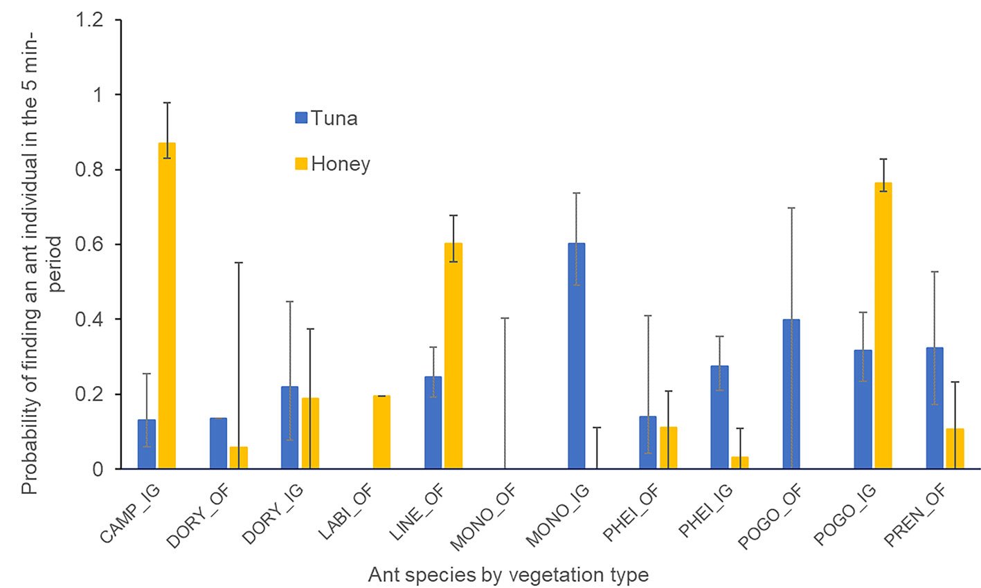
Figure 3. Probability of finding an ant forager on the honey or tuna baits at the nest of the different ant species registered in the Oak Forest (OF) and the Induced Grassland (IG) in the 5-minute period. CAMPO: Camponotus rubrithorax, DORY: Dorymyrmex insanus, LABI: Labidus coecus, LINE: Linepithema dispertitum, MONO: Monomorium ebenium, PHEI: Pheidole spp., POGO: Pogonomyrmex barbatus, PREN: Prenolepis imparis.

Figure 4. Survival curves depicting the arrival times of ant foragers on the baits (tuna or honey) during a one-hour observation.
No significant differences were found in the arrival times among ant species.
No significant differences were found in the arrival times between the vegetation types (x2 = 0.4, df = 1, p = 0.5). Moreover, no significant differences were found in the arrival times among the different ant species (x2 = 7.6, df = 7, p = 0.4) or the type of bait (x2 = 0.01, df = 1, p = 0.9; Fig. 4).
In the dominance index baits 12 ant morphospecies were recorded and different ant morphospecies were recorded in each of the vegetation types (Table 3). When comparing the average dominance index (DI) by vegetation type (mean ± SE, n; oak forest DI = 0.372 ± 0.071, 33; induced grassland DI = 0.251 ± 0.052, 44), was not statistically different (t= 1.091; df = 75; p = 0.2787), which would suggest a submissive behavior in both types of vegetation. Average dominance index by ant species indicates that M. ebenium, P. imparis and Pheidole sp. 3 behave as submissive in both vegetation types (t = 0.590, df = 20, p = 0.5617; t = -0.237, df = 10, p = 0.8171; t = -0.315, df = 11, p = 0.7590, respectively) (Table 4). It was not possible to compare the DI between vegetation types for Temnothorax sp., T. augusti, C. rubrithorax, N. austroccidua, L. dispertitum, D. insanus or P. pallidus, because they were only present in one of the vegetation types (Table 4).
The average dominance index for each ant species was low suggesting that all of them displayed submissive behaviors (F8,68 = 1.949, p = 0.06). Nylanderia austroccidua and L. dispertitum had the highest dominance indices, although it should be noted that N. austroccidua only had one record and L. dispertitum had 3 records. Additionally, Monomorium ebenium showed a tendency to behave as dominant (Table 4).
When comparing the mean dominance index by bait type, no significant differences were found (t = 1.023, df = 110, p = 0.3088; mean ± SE, n; tuna = 0.382 ± 0.060, 55; honey = 0.295 ± 0.053, 57). This indicates that ants exhibited submissive behavior in both types of bait.
According to the average dominance index per ant species in relation to the bait type, Pheidole sp. 3, P. imparis, M. ebeninum, C. rubrithorax, and D. insanus exhibited a submissive behavior in both types of baits (t = 0.888, df = 13, p = 0.3907; t= 0.988, df = 15, p = 0.3388; t = 0.189, df = 32, p = 0.8513; t = -0.918, df = 24, p = 0.3675, t = 2.390, df = 5, p = 0.0624, respectively) (Table 5) and L. dispertitum exhibited a dominant behavior in both types of baits (t = 0.421, df = 3, p = 0.7021).
Temnothorax sp. and P. pallidus were not compared statistically due to the low incidence registered; nonetheless, they presented a submissive behavior index in both types of bait. Neither T. augusti nor N. austroccidua were included in this analysis, as they were only present on the honey bait. In none of the species was there a difference in behavior between the baits.
Table 2
Number of nests found in the oak forest and the induced grassland.
| Species | Oak forest | Induced grassland |
| Camponotus rubrithorax | 0 | 3 |
| Dorymyrmex insanus | 4 | 6 |
| Labidus coecus | 1 | 0 |
| Linepithema dispertitum | 2 | 0 |
| Pheidole spp. | 7 | 6 |
| Pogonomyrmex barbatus | 1 | 2 |
| Prenolepis imparis | 3 | 0 |
| Monomorium ebenium | 1 | 1 |
Discussion
This study found that certain ant species (e.g., C. rubrithorax, L. dispertitum, P. barbatus) exhibited a preference for honey within specific vegetation types when compared to the rest of the ant community. The compensation hypothesis (Davidson, 2005; Kaspari & Yanoviak, 2001) predicts that the attractiveness of a nutrient to an organism is higher the more limiting it is. It is possible that this result is related to the fact that sugar is generally less available on the ground strata than protein (Kaspari & Yanoviak, 2001; Kaspari et al., 2012).
However, when considering the overall community level, no noticeable food preferences were found between the ant communities in the oak forest and the induced grassland vegetation. This lack of preference was evident both in the items carried to their nests and the resources provided on the baits. There were no significant differences in arrival times at the baits between vegetation types. This similarity can be attributed to ants experiencing soil-level heterogeneity similarly in both oak forests and induced grasslands (see below).
The ant communities in both habitats were composed of ant species displaying submissive behavior. This characteristic could be attributed to stress factors such as low temperatures in the oak forest and disturbances in the induced grassland, which potentially reduce ant competition. In the oak forest, low temperatures may favor the presence of cold climate specialists that can forage at low temperatures without the need to display a dominant behavior. In the induced grassland, disturbances may favor the presence of generalist species that take advantage of the absence of dominant species such as the dominant Dolichoderinae (see below). This study emphasizes the significance of ant species’ response to their environment and their adaptability in dealing with disturbances.
Our findings do not provide support for vegetation-scale disparities in food preferences, first and second hypotheses, which proposed greater differences in the food items being carried to the nest in the oak forest and reduced food preferences in the induced grassland. There were no differences between vegetation types in the number of seeds, plants, or arthropods taken by the ant foragers to their nests. Similarly, there was not a preference for a specific food bait (honey or tuna) between the oak forest and induced grassland ant communities. These findings are consistent with previous studies conducted by Radnan et al. (2018) and Castillo-Guevara et al. (2019), which did not identify differences in food preferences or foraging strategies between natural and disturbed vegetation at the community level. However, our observations did reveal that certain ant species exhibited preferences for specific types of food, within particular vegetation types, in accordance with the first hypothesis and second hypothesis but at the species level, which proposed an influence of ant species on food preferences. The specific preferences of these ant species are discussed in detail below.
Table 3
Visit frequency (i.e., number of foragers) per species in each vegetation type and functional groups they belong to (Andersen, 2000). GM = Generalized Myrmicinae, CCS = cold climate specialist, SC = subordinate Camponotini, TCS = tropical climate specialist, O = opportunist.
| Subfamily | Specie | Funtional group | Oak forest | Induced grassland |
| Myrmicinae | Monomorium ebenium | GM | 753 | 167 |
| Myrmicinae | Pheidole sp. 3 | GM | 14 | 236 |
| Myrmicinae | Temnothorax sp. | CCS | 5 | 0 |
| Myrmicinae | Temnothorax augusti | CCS | 0 | 1 |
| Formicinae | Prenolepis imparis | CCS | 289 | 11 |
| Formicinae | Camponotus rubrithorax | SC | 0 | 351 |
| Formicinae | Nylanderia austroccidua | TCS | 0 | 30 |
| Dolichoderinae | Linepithema dispertitum | CCS | 190 | 0 |
| Dolichoderinae | Dorymyrmex insanus | O | 0 | 26 |
| Pseudomyrmecinae | Pseudomyrmex pallidus | TCS | 0 | 10 |
| Total | 1,251 | 832 |
Table 4
Average numerical dominance index (DI) (mean ± SE, n) per ant morphospecies. (-) Unregistered species.
| Specie | Oak forest | Induced grassland | ID |
| Monomorium ebenium | 0.4 ± 0.1, 13 | 0.3 ± 0.1, 9 | 0.4 ± 0.0, 22 |
| Pheidole sp.3 | 0.2 ± 0.2, 4 | 0.2 ± 0.1, 9 | 0.2 ± 0.1, 13 |
| Temnothorax sp. | 0 ± 0, 3 | – | 0 ± 0, 3 |
| Temnothorax augusti | – | 0, 1 | 0 ± 0, 1 |
| Prenolepis imparis | 0.3 ± 0.1, 10 | 0.5 ± 0.5, 2 | 0.3 ± 0.1, 12 |
| Camponotus rubrithorax | – | 0.1 ± 0.0, 15 | 0.1 ± 0.0, 15 |
| Nylanderia austroccidua | – | 1, 1 | 1, 1 |
| Linepithema dispertitum | 0.7 ± 0.1, 3 | – | 0.7 ± 0.1, 3 |
| Dorymyrmex insanus | – | 0.2 ± 0.1, 4 | 0.3 ± 0.1, 4 |
| Pseudomyrmex pallidus | – | 0 ± 0, 3 | 0 ± 0, 3 |
Pheidole spp., in the induced grassland, were observed carrying a greater quantity of plant elements to their nests in both vegetation types. However, it exhibited a preference for the tuna bait in induced grassland, possibly indicating a supplementary dietary preference. Given the extensive diversity within the Pheidole genus, which encompasses 900 species described worldwide (Wilson, 2003), it is not feasible to categorize them based on a specific food habit and our results suggest that it is omnivorous (Table 6). Nevertheless, these results should be interpreted with caution due to the grouping of species.
Camponotus rubrithorax and P. barbatus, in the induced grassland, as well as L. dispertitum, in the oak forest, were more frequently observed foraging the honey bait compared to other ant species. Camponotus (Mayr) is a genus known for its nectarivorous habits and consumption of other sweet secretions, such as honeydew which coincides with its preference for honey found in the present study (Nettimi & Iyer, 2015). In this study, L. dispertitum predominantly consumed honey, although it is a generalist forager species capable of consuming other types of food as well (Table 5), in the study site it is found exclusively in the oak forest (Cuautle et al., 2016).
Despite Pogonomyrmex (Mayr) has been recognized as a granivorous genus (Pirk & López-de Casenave, 2014), this study provided new insights into the foraging preferences of P. barbatus, revealing a notable inclination towards carbohydrates and plant elements within the induced grassland. Moreover, we even registered individuals transporting arthropods to their nests. These findings (Table 5) strongly indicate that certain species within the Pogonomyrmex genus exhibit a generalist foraging behavior. Other species such as D. insanus, which used resources more intensively in the induced grassland, showed no preference for any of the baits or items taken to the nest, which coincides with the generalist forager behavior, observed in open and disturbed habitats by Cuezzo and Guerrero (2012).
Table 5
Average numerical dominance index (DI) (mean ± SE, n) per ant species in both bait types (tuna, honey). (-) Unregistered species.
| Species | Tuna | Honey |
| Monomorium ebenium | 0.4 ± 0.1, 18 | 0.4 ± 0.1, 16 |
| Pheidole sp.3 | 0.4 ± 0.2, 7 | 0.1 ± 0.1, 8 |
| Temnothorax sp. | 0, 1 | 0 ± 0, 2 |
| Temnothorax augusti | – | 0, 1 |
| Prenolepis imparis | 0.5 ± 0.1, 7 | 0.3 ± 0.1, 10 |
| Camponotus rubrithorax | 0.1 ± 0.0, 14 | 0.2 ± 0.0, 12 |
| Nylanderia austroccidua | – | 1, 1 |
| Linepithema dispertitum | 0.7 ± 0.2, 2 | 0.6 ± 0.3, 3 |
| Dorymirmex insanus | 0.6 ± 0.3, 3 | 0 ± 0, 4 |
| Pseudomyrmex pallidus | 0 ± 0, 3 | 0, 1 |
Table 6
The biology and ecology of the ant genera found in this study, in the Flor del Bosque State Park (Agosti et al., 2000; AntWiki, n.d.).
| Genera | Microhabitat | Food habits |
| Camponotus | Ground nesting, decaying wood and in trees | Generalist foragers |
| Dorymyrmex | ————– | Generalist foragers |
| Linepithema | ————– | Generalist foragers |
| Labidus | Epigeous,bivouacs | Predators (Army ants) |
| Monomorium | ————– | Generalized foragers, harvesters |
| Nylanderia | Nest in leaf litter, soil, or in rotten wood | Generalist foragers |
| Pheidole | Soil or decaying wood | Granivores or omnivores |
| Pogonomyrmex | Ground nesting | Generalist foragers and granivores |
| Prenolepis | ————– | Generalist predators |
| Pseudomyrmex | Mostly arboreal (nesters and foragers), few epigaeic | Generalized predators, visit extrafloral nectaries |
| Temnothorax | Nesting in ground, and under stones, in wood, and in trees | Generalized foragers and parasites |
The previous results (e.g., C. rubrithorax, Pheidole spp., D. insanus) support the reported food habits of specific ant genera. Nonetheless, it is also possible to interpret these results as ants taking nutrients from the baits that are not currently available or that are limited within their community to supplement their diet (Compensation hypothesis) (Davidson, 2005; Kaspari & Yanoviak, 2001). In this study, significant differences in ant species presence on baits were primarily associated with the presence of ant species on honey baits. This finding aligns with the compensation hypothesis (Davidson, 2005; Kaspari & Yanoviak, 2001), which posits that the utility of a resource remains constant across species and varies solely with availability. The hypothesis predicts a singular limiting resource that is locally in shortest supply. Consequently, habitats with relatively high protein availability should attract ants more inclined towards carbohydrates, and vice versa. Previous research has demonstrated that litter ant communities are limited by carbohydrates, whereas ant arboreal communities face protein limitations in tropical regions (Kaspari & Yanoviak, 2001; Kaspari et al., 2012). Although this study was conducted in a temperate environment, the results might be related to the usual scarcity of sugar in the ground strata compared to protein.
Our results do not align with the second hypothesis, which speculated faster arrival times in the induced grassland. We did not find significant differences in arrival times among vegetation types, ant species, or bait types. Ants could be experiencing similar heterogeneities at the soil level between the oak forest and induced grassland. While it is expected that the presence of more litter in the oak forest could hinder ant movement, within the induced grassland, the vegetation morphology itself (long grass species) could be interfering with ant movement. For instance, Hernández-Flores et al. (2016) observed that the foraging performance of P. barbatus was reduced due to the presence of herbaceous vegetation in plots where regeneration after grazing was permitted.
Dominance hierarchy. Disturbance typically favors the presence of generalist and opportunistic species, hence, we expected to find a lower dominance index within the induced grassland (third hypothesis). Nonetheless, we did not find enough evidence to support this hypothesis as we registered ant communities consisted of submissive species in both habitats. Additionally, the ants did not show a tendency to dominate a specific resource, neither at the bait level nor at the species level, suggesting a lack of food preferences. These results are consistent with the findings of Castillo-Guevara et al. (2019), who registered no significant differences in dominance indices between a native oak forest and an altered agricultural land. Moreover, the authors reported intermediate to low values of dominance within the ant communities of each vegetation type. Our findings could be attributed to the presence of other factors that could have overshadowed the role of competition in shaping the organization of ant communities. For example, a review by Parr and Gibb (2012), which encompassed data from 3 continents, indicated that the trade-off between discovery and dominance occurs primarily when parasitoids are present. In environments without parasitoids, species with high discovery abilities tend to also be dominant (Parr & Gibb, 2012). While our study did not specifically assess the discovery-dominance trade-off, the observed lack of differences in arrival times and similar dominance values among the ants suggest that dominance was not a prominent factor in our study sites. It is possible that factors such as low temperatures in the oak forest, or disturbance in the induced grassland, may have played a role in relaxing dominance. According to Andersen (2000), in disturbed vegetation like the induced grassland, it is expected to observe the presence of subdominant ant species that exploit the absence of dominant species from the native vegetation, such as dominant Dolichoderinae. The findings obtained during this study align with this prediction and provide support for it. Notwithstanding, the absence of ants with high dominance indices in the studied communities does not necessarily indicate a complete lack of dominance hierarchy. In each community, the ants can still be ordered based on their DI. For example, in the oak forest, L. dispertitum had the highest DI value (0.7 DI), M. ebenium had an intermediate value (0.4 DI) and Temnothorax spp. had the lowest value (0.0 DI).
Land use change did not seem to influence food preferences or foraging strategies at the community level. However, we observed an effect at species level, indicating that individual ant species exhibited specific food preferences. Carbohydrates could be the limiting resource in the oak forest and the induced grassland litter ant communities, as some ant species showed preference for honey baits. Although competition is typically considered a key factor in understanding food preferences among ants, it is noteworthy that both, the natural oak forest and induced grassland, were predominantly populated by submissive ant species. Therefore, it appears that other factors instead of competition may be playing a role in shaping food preferences within these communities. In conclusion, our study reveals that ant species may exhibit preferences for specific foods, which could be limited in their environment. The ability of ants to respond to available resources enables them to optimize their nutrient intake, as well as adapt and persist under variable conditions, including disturbances. Understanding the distinct dietary preferences and foraging strategies of ant species within functional groups will provide valuable insights into their ecological roles and potential impacts on ecosystem dynamics. Such investigations would enhance our ability to predict the responses of ants to diverse forms of disturbances in an anthropized world.
Acknowledgements
We appreciate the assistance provided by the authorities of “Flor del Bosque” State Park, coordinator Enrique Martínez Romero (M.S.) and director Mario Alberto Romero Guzmán (MVZ). We would also like to thank Florencio Luna Castellanos for his support with the fieldwork. This study was financed by Consejo Nacional de Humanidades Ciencias y Tecnologías (Conahcyt) as part of a grant awarded to Mariana Cuautle (223033).
References
Abacus Concepts Inc. (1996). Abacus Concepts, Stat View Reference. Berkeley, California.
Agosti, D., Majer, J. D., Alonso, L. E., & Schultz, T. R. (2000). Ants: standard methods for measuring and monitoring bio-
diversity. Washington D.C.: Smithsonian Institution Press.
Andersen, A. (2000). A global ecology of rainforest ants: functional groups in relation to environmental stress and disturbance. In D. Agosti, J. D. Majer, L. E. Alonso, & T. R. Schultz (Eds.), Ants: standard methods for measuring and monitoring biodiversity (pp. 25–34). Washington D.C.: Smithsonian Institution Press.
Andersen, A.N. (1992). Regulation of “momentary” diversity by dominant species in exceptionally rich ant communities of the Australian seasonal tropics. The American Naturalist, 40, 401–420. https://www.journals.uchicago.edu/doi/abs/10.
1086/285419
AntWiki (n.d.). Nylanderia. AntWiki. Consulted 8/20/2024
Arnan, X., Cerdá, X., & Retana, J. (2012). Distinctive life traits and distribution along environmental gradients of dominant and subordinate Mediterranean ant species. Oecologia, 170, 489–500. https://doi.org/10.1007/s00442-012-2315-y
Castillo-Guevara, C., Cuautle, M., Lara, C., & Juárez-Juárez, B. (2019). Effect of agricultural land-use change on ant dominance hierarchy and food preferences in a temperate oak forest. PeerJ, 7, e6255. https://peerj.com/articles/6255/
Cerdá, X., Arnan, X., & Retana, J. (2013). Is competition a significant hallmark of ant (Hymenoptera: Formicidae) ecology? Myrmecological News, 18, 131–147. https://doi.org/10.25849/myrmecol.news_018:131
Cerdá, X., Retana, J., & Cros S. (1997). Thermal disruption of transitive hierarchies in Mediterranean ant communities. Journal of Animal Ecology, 66, 363–374.
Costes-Quijano, R., Meza, A. R., Macías-Juárez, A., Berriel-Mastreta, C. A., Cortés-Atilano, B., Martínez-Romero, L. E. et al. (2006). Plan de manejo Parque Ecológico Recreativo General Lázaro Cárdenas “Flor del Bosque”. [Management Plan of the recreative ecological Park “General Lázaro Cárdenas “Flor del Bosque”]. Ciudad de México: Gobierno del Estado de Puebla/ Secretaría de Medio Ambiente y Recursos Naturales.
Cuautle, M., Vergara, C., & Badano, E. (2016). Comparison of ant community diversity and functional group composition associated to land use change in a seasonally dry oak forest. Neotropical Entomology, 45, 170–9. https://doi.org/
10.1155/2012/516058
Cuezzo, F., & Guerrero, R. J. (2012). The Ant Genus Dorymyrmex Mayr (Hymenoptera: Formicidae: Dolicho-
derinae) in Colombia. Psyche, 51605, 1–24. https://doi.org/
10.1155/2012/516058
Dáttilo, W., Díaz-Castelazo, C., & Rico-Gray, V. (2014). Ant dominance hierarchy determines the nested pattern in ant-plant networks. Biological Journal of the Linnean Society, 113, 405–414. https://doi.org/10.1111/bij.12350.
Davidson, D. W. (2005). Ecological stoichiometry of ants in a New World rain forest. Oecologia, 142, 221–231. https://doi.org/10.1007/s00442-004-1722-0
Dejean, A., & Corbara, B. (2003). A review of mosaics of dominant ants in rainforests and plantations. In Y. Basset, V. Novotny, S. E. Miller, & R. L. Kitching (Eds.), Arthropods of tropical forests: spatio-temporal dynamics and resource use in the canopy (pp 341–347). Cambridge: Cambridge University Press.
Ellis, E. C., Goldewijk, K. K., Siebert S., Lightman, D., & Ramankutty, N. (2010). Anthropogenic transformation of
the biomes, 1700 to 2000. Global Ecology and Biogeo-
graphy, 19, 589–606. https://doi.org/10.1111/j.1466-8238.20
10.00540.x
Fellers, J. H. (1987). Interference and exploitation in a guild of Woodland ants. Ecology, 68, 1466–1478. https://doi.org/
10.2307/1939230
Fellers, J. H. (1989). Daily and seasonal activity in woodland
ants. Oecologia, 78, 69–76. https://doi.org/10.1007/BF0037
7199
Foley, J. A., DeFries, R., Asner, G. P., Barford C., Bonan, G., Carpenter, S. R. et al. (2005). Global consequences of land use. Science, 309, 570–574. https://doi/10.1126/science.1111772
Hoffmann, B. D., & Andersen, A. N. (2003). Responses of ants to disturbance in Australia, with particular reference to functional groups. Austral Ecologyl, 28, 444–464. –https://doi.org/10.1046/j.1442-9993.2003.01301.x
Houdria, M., Salas-López, A., Orivel. J., Bluthgen, N., & Menzel, F. (2015). Dietary and temporal niche differentiation in tropical ants – can they explain local ant coexistence? Biotropica, 47,208–217. https://doi.org/10.1111/btp.12184
Hernández-Flores, J., Osorio-Beristain. M., & Martínez-Garza. C. (2016). Ant foraging as an indicator of tropical dry forest restoration. Environmental Entomology, 45, 991–994. https://doi.org/10.1093/ee/nvw054
Kaspari, M., Donoso, D., Lucas, J. A., Zumbusch, T., & Kay, A. D. (2012). Using nutritional ecology to predict community structure: a field test in Neotropical ants. Ecosphere, 3,93. https://doi.org/10.1890/ES12-00136.1
Kaspari, M., & Yanoviak, S. P. (2001). Bait use in tropical litter and canopy ants-evidence of differences in nutrient limitation. Biotropica, 33,207–211. https://doi.org/10.1646/
0006-3606(2001)033[0207:BUITLA]2.0.CO;2
Łaska, G. (2001). The disturbance and vegetation dynamics: a review and an alternative framework. Plant Ecology, 157, 77–99. https://doi.org/10.1023/A:1013760320805
Lynch, J. F., Balinsky, E. C., & Vail, S. G. (1980). Foraging patterns in three sympatric forest ant species, Prenolepis imparis, Paratrechina melanderi and Aphaenogaster rudis (Hymenoptera: Formicidae). Ecological Entomology, 5,353–371. https://doi.org/10.1111/j.1365-2311.1980.tb01160.x
Mackay, W., & Mackay, E. (1989). Clave de los géneros de hormigas en México (Hymenoptera: Formicidae). El Paso, Texas: The University of Texas.
Nettimi, R. P., & Iyer, P. (2015). Patch fidelity in Camponotus compressus ants foraging on honeydew secreted by treehoppers. Current Science, 109, 362–366.
Parr, C. L. (2008). Dominant ants can control assemblage species richness in a South Africa savanna. Journal of Animal Ecology, 77, 1191–1198. https://doi.org/10.1111/j.13
65-2656.2008.01450.x
Parr, L., & Gibb, H. (2012). The discovery-dominance trade-off
is the exception, rather than the rule Journal of Animal
Ecology, 81, 233–241. https://doi.org/10.1111/j.1365-2656.
2011.01899.x
Pirk, G. I., & López-de Casenave, J. (2014). Effect of harvester ants of the genus Pogonomyrmex on the soil seed bank around their nests in the central Monte desert, Argentina. Ecological Entomology, 39, 610–619. https://doi.org/10.1111/een.12140
R Core Team (2022). R: a language and environment for statistical computing. Vienna, Austria: R Foundation
for Statistical Computing. https://www.R-project.org/
Radnan, G. N., Gibb, H., & Eldridge, D. J. (2018). Soil surface complexity has a larger effect on food exploitation by ants than a change from grassland to shrubland. Ecological Entomology, 43, 379–388. https://doi.org/10.1111/een.12510
Rico-Gray, V., & Oliveira, P. S. (2007). The ecology and evolution of ant-plant interactions. Chicago: University of Chicago Press.
Sala, O. E., Chapin, F. S., Armesto, J. J., Berlow, E., Bloomfield, J., Dirzo. R. et al. (2000). Global biodiversity scenarios for the year 2100. Science, 287,1770–1774. https://doi.org/10.1126/science.287.5459.17
Santini, G., Tucci, L., Ottonetti, L., & Frizzi, L. (2007). Competition trade-offs in the organisation of a Medite-
rranean ant assemblage. Ecological Entomology, 32,
319–326. https://doi.org/10.1111/j.1365-2311.2007.00882.x
Savolainen, R., Vepsäläinen, K., & Wuorenrinne, H. (1989). Ant assemblages in the taiga biome: testing the role of territorial wood ants. Oecologia, 81, 481–486. https://doi.org/10.1007/BF00378955

The sounds of love: acoustic repertoire of Andean bear, Tremarctos ornatus (Carnivora: Ursidae), mating in the wild
Adriana Reyes a, b, Nicolás Reyes-Amaya a, b, Ramiro Velazco c, Manuel Meneses c, Andrés Cortés e, Katherine Arenas-Rodríguez d, Edward Rojas e, Ximena Velez-Liendo f, Angela M. Mendoza-Henao a, *
a Instituto de Investigación de Recursos Biológicos Alexander von Humboldt, Centro de Colecciones y Gestión de Especies, Colecciones Biológicas, Carrera 8 No. 15 – 08, 154001 Villa de Leyva, Colombia
b Fundación para la Investigación, Conservación y Protección del Oso Andino (Fundación Wii), Calle 161, 12C-30, 110131 Bogotá, Colombia
c Grupo de monitoreo comunitario Serankwa, Vereda Candela, San Agustín, Huila, Colombia
d Corporación Autónoma Regional del Alto Magdalena, Carrera 1 No. 60-70, Neiva, 41797 Huila, Colombia
e Corporación Autónoma Regional de Cundinamarca, Dirección Recursos Naturales, Calle 24 No. 60-50, Bogotá, Colombia
f University of Oxford, Department of Biology, Wildlife Conservation Research Unit, Recanati-Kaplan Centre, Tubney House Abingdon Road, Tubney, Oxfordshire, OX13 5QL United Kingdom
*Corresponding author: am.mendozah@gmail.com (A.M. Mendoza-Henao)
Received: 14 March 2024; accepted: 11 October 2024
Abstract
Understanding animal behavior is crucial for effective mammal conservation efforts; however, limited knowledge exists regarding the behavioral patterns of many species, particularly in wild conditions. The Andean bear (Tremarctos ornatus) is the only ursid distributed in South America and is categorized as vulnerable to extinction by the IUCN. The information on various aspects of its natural history in wildlife conditions are scarce, including the ethology of its reproduction. In this study, we describe the sound repertoire emitted by T. ornatus during copulation and mating events in their natural habitat. Video recordings obtained from camera traps in Colombia and Bolivia were analyzed to identify and categorize vocalizations. The results revealed 5 distinct types of sounds emitted during copulation events: humm, grunt, whine, and snoar signals. Differences in vocalization patterns were observed between the male and female bears. Comparisons with existing literature suggest similarities with the vocalizations observed for other species. This study contributes valuable information to the understanding of Andean bear behavior and underscores the importance of acoustic communication in conservation efforts for cryptic species.
Keywords: Camera trapping; Colombia; Bolivia; Bioacoustics; Reproductive behaviour
© 2025 Universidad Nacional Autónoma de México, Instituto de Biología. Este es un artículo Open Access bajo la licencia CC BY-NC-ND
(http://creativecommons.org/licenses/by-nc-nd/4.0/).
Sonidos amor-osos: repertorio acústico del oso andino Tremarctos ornatus (Carnivora: Ursidae) durante el apareamiento en vida silvestre
Resumen
Comprender el comportamiento de los animales es crucial para que los esfuerzos de conservación de los mamíferos sean eficaces, pero los conocimientos sobre los patrones de comportamiento de muchas especies, sobre todo en condiciones salvajes, son limitados. El oso andino (Tremarctos ornatus) es el único úrsido distribuido en Sudamérica, categorizado como vulnerable a la extinción por la UICN. La información sobre diversos aspectos de su historia natural en vida silvestre es escasa, incluyendo la etología de su reproducción. En este estudio describimos el repertorio sonoro emitido durante los eventos de cópula y apareamiento por T. ornatus en su hábitat natural. Se analizaron grabaciones de vídeo obtenidas con cámaras trampa en Colombia y Bolivia para identificar y categorizar las vocalizaciones. Los resultados revelan 5 tipos distintos de sonidos emitidos durante los eventos de cópula, incluyendo señales de “humm”, “grunt”, “whine” y “snoar”. Se observaron diferencias en los patrones de vocalización entre machos y hembras. Las comparaciones con la literatura existente sugieren similitudes con las vocalizaciones observadas en otras especies. Este estudio contribuye con información valiosa a la comprensión del comportamiento del oso andino y subraya la importancia de la comunicación acústica en los esfuerzos de conservación de especies crípticas.
Palabras clave: Fototrampeo; Colombia; Bolivia; Bioacústica; Comportamiento reproductivo
Introduction
The study of animal behavior plays a fundamental role in mammalian conservation, as it provides valuable information on the relationships between species and their environment (Berger-Tal et al., 2016). Understanding species behavioral patterns is crucial for designing effective conservation strategies, as it allows scientists to identify and address key factors influencing population dynamics, habitat utilization, and overall ecological balance. A thorough understanding of animal behavior is essential for developing informed and adaptive conservation practices that safeguard species diversity. In many cases, knowledge of the behavior of wild species of large mammals comes from captive conditions (Jayne & See, 2019). Although captivity provides a controlled environment for observation, it can inadvertently influence animal behavior. Captive individuals exhibit altered behaviors as they are subjected to artificial conditions, restricted spaces, and stimuli provided by humans. This can lead to biased results that do not accurately reflect the natural behavior of their wild counterparts. Even so, information on wild conditions is scarce for many species, considering the difficulties in directing encounters without altering individual behavior.
Few studies have focused on the social behavior and vocalizations of ursids (Wemmer et al., 1976). The first studies on this subject were done by Meyer-Holzapfel (1957), who mentioned several calls of different species; Krott and Krott (1962) described the vocalizations of the European brown bear (Ursus arctos, Carnivora: Ursidae), and Jonkel (1970), Jonkel and Cowan (1971) described calls used in agonistic contexts by North American bears, while Negus (1949) in his study of the vertebrate larynx reported that bears are generally silent.
Fortunately, advances in remote sensing technologies have provided us with opportunities to explore animal behavior. The scarcity of information on the ecology of the Andean bear has been changing in recent years owing to the use of tools such as camera traps, which have allowed us to obtain more information about the species, and the recording of various behaviors such as courtship, maternal care, and copulation events has been achieved (Appleton et al., 2018; Castellanos, 2015; Reyes et al., 2018, 2024). The objective of this study was to describe the vocalizations emitted by Andean bears during copulation events in the wild.
Materials and methods
Video records were obtained using camera traps during the copulation of wild bears in 3 locations: 2 in Colombia and 1 in Bolivia (Fig. 1). The first was in the Department of Huila (Colombia): the mating event was recorded by the SERANKWA monitoring group in a Cuddeback camera trap located in the site called “El Rascadero” (1°49’35.06” N, 76°23’35.41” W, WGS84), in the Natural Reserve of the Civil Society La Loma del Toro Pao in the Municipality of San Agustín at 2,410 m asl, the reserve has areas of forest cover in good condition (Parques Nacionales Naturales de Colombia, 2017). The second locality was in the department of Cundinamarca (Colombia): this mating event was recorded by the Corporación Autónoma Regional de Cundinamarca- CAR, Dirección de Recursos Naturales, Grupo de Biodiversidad in 2 camera traps (Bushnell Trophy Cam HD) in the municipality of Guatavita (4°54’0.06” N; 73°44’21.56” W and 4°53’58.65” N, 73°43’40,47” W, WGS84), in the Eastern Cordillera (Anillo Oriental) of the Colombian Andes in the buffer zone of Chingaza Natural Park, which includes Andean and high Andean forests between 2,500 and 3,000 m asl. The third locality is in Tarija department (Bolivia): mating event was recorded in 2 camera traps (Bushnell Trophy Cam HD Aggressor) 15.8 km from Hoyadas Cercado, Cercado Province (21°7’29.10” S, 64°25’16.90” W and 21°14’39.00” S, 64°20’12.90” W, WGS84), between 930 and 3,400 m asl.

Figure 1. Location of study sites. A) El Rascadero, Huila, Colombia; B) Chingaza, Cundinamarca, Colombia; C) Cercado, Tarija, Bolivia. Map by Angela M. Mendoza-Henao.
The videos were manually examined to identify those with vocalizations and, to the extent possible, to assign the signal to the male or female. WAV files were generated from the selected videos. Information on the times of vocal activity was obtained from camera trap metadata. Acoustic parameters were obtained using Raven 1.6.2 (K. Lisa Yang Center for Conservation Bioacoustics): call duration, minimum and maximum frequency were obtained using 5% and 95% values with a window size of 1,024 and a Hann algorithm. The final recordings were deposited in the Colección de Sonidos Ambientales “Mauricio Álvarez-Rebolledo” of the Instituto de Investigación de Recursos Biológicos Alexander von Humboldt of Colombia (IAvH-CSA-37506 to IAvH-CSA-37510). The vocalization parameters were summarized and described for each event.
Results
Vocalizations or sounds were obtained from the 6 copulation events analyzed (3 from Colombia and 3 from Bolivia), with some differences in audio quality due to the camera trap brands and models, and the distance of the individuals from the equipment. During the analysis, we were able to classify 5 different types of sounds according to the shape of the spectrogram (Table 1), following the terminology of vocalization descriptions of other ursids (Peters et al., 2007; Pokrovskaya, 2013).
Regarding the Cundinamarca events in Colombia, mating occurred on September 14, 2021, between 11:36 and 12:33 hrs. (camera 4), and between 14:24 and 15:51 hrs. (camera 5). Acoustic signals were detected in 55 videos from both sites (Fig. 2). All the sounds recorded were presented when the male is on the female, in the videos it is observed how both the male and the female emit different sounds in the process of copulation. In general, all the recorded sounds are of the copulation process. A total of 33 sounds between vocalizations and snorts were emitted by females and 48 by males. For the remaining vocalizations, individual correspondence could not be verified. The bears mostly emitted humm-type vocalizations, which in some cases were preceded or followed by other types of vocalizations. During the time of copulation, both videos and sounds show some moments of aggressiveness of the male towards the female, this is evident in an event where the male bites the neck of the female and she emits a very high-pitched sound (bite-type vocalization, Fig. 2). Table 2 summarizes the main quantified parameters of the signals.
For events in Bolivia, 2 videos from station PI072 included sound information (Fig. 3a). The recorded vocalizations included humm, grunt and whine signals emitted simultaneously by males and females. Snort-type vocalizations were dominant in both the recordings. These recordings provided information on frequencies below 5 kHz, and harmonics up to 10.16 kHz in frequency were detected. Four of the videos from station PI012 included sounds from a single individual in sight (Fig. 3b), recorded at 6:42 am and between 10:37 am and 10:41 am. All signals were humm with 9 – 22 pulses with a dominant frequency at 344.53 ± 54.47 Hz and a second harmonic frequency with the highest energy at 6,488.67 ± 611.07 Hz with frequencies covering a bandwidth of 8,641.99 ± 886.23 Hz. The mean signal duration was 1.035 ± 0.33 s. Finally, a single video from station PI071 from 2022-10-29 includes a series of sounds made by a single individual (sex unknown, Fig. 3c) including humm (dominant frequency of 301.46 Hz and duration of 0.96 s), whine (dominant frequency of 172.2, duration of 3.52 s) and snoar (dominant frequency at 3,200 Hz for 2 signals and 872.1 for the remaining 4, total duration of 0.255 s) type signals.

Figure 2. Spectrograms of the 6 types of Tremarctos ornatus signals emitted during the mating event in Cundinamarca, Colombia.
The mating event in Huila (Colombia) occurred on February 9, 2020, between 08:14 and 13:03 hrs. The second copulation event was recorded at the same site on February 13, 2020, between 14:05 and 17:17 hrs. (56 videos and 49 photographs). The camera had a sound filter above 5 kHz, which limited the availability of data beyond this frequency. Acoustic signals were detected in only 28 of 122 videos. Five videos in the interval between the 2 mating events also had acoustic signals. Owing to the sound quality of the camera and the distance of the pair, the signal was sufficient in only 1 video to extract some spectral parameters (Fig. 4). In this case, the call was probably a 2.196 second humm-type vocalization, with frequencies between 1,125.0 and 1,843.75 Hz (dominant frequency 1,625.00 Hz).
Table 1
Description of the type of acoustic signals of Tremarctos ornatus during courtship and copulation events and spectrogram example of each one (1 second section).

Table 2
Summary of the main signal parameters for mating in Cundinamarca (Colombia). Spectral values are given in Hz and signal duration in seconds. Values for more than 3 signals mean ± standard deviation.
| Type | Sex | N | Dom freq | Min freq | Max freq | Freq bandwidth | Signal duration |
| Bite | F | 2 | 1,679.55 ± 1,888.05 | 301.45 ± 121.83 | 2,045.65 ± 1,979.40 | 1,744.20 ± 1,857.57 | 0.550 ± 0.495 |
| NA | 2 | 344.50 ± 0.00 | 193.80 ± 30.41 | 925.95 ± 700.39 | 732.15 ± 730.79 | 1.650 ± 0.071 | |
| Grunt | M | 8 | 220.70 ± 101.49 | 134.58 ± 104.09 | 613.70 ± 713.54 | 479.13 ± 610.10 | 0.213 ± 0.164 |
| NA | 14 | 196.88 ± 62.55 | 153.81 ± 43.78 | 310.69 ± 117.26 | 156.88 ± 90.36 | 0.407 ± 0.327 | |
| Whine | F | 5 | 516.78 ± 337.73 | 353.14 ± 47.19 | 1,326.44 ± 315.59 | 973.30 ± 309.94 | 0.420 ± 0.409 |
| NA | 41 | 259.45 ± 101.22 | 199.58 ± 73.82 | 638.65 ± 627.49 | 439.06 ± 589.26 | 0.478 ± 0.442 | |
| Humm | F | 25 | 821.70 ± 1,090.34 | 246.35 ± 82.02 | 2,322.15 ± 1,024.95 | 2,075.80 ± 1,002.38 | 2.112 ± 1.568 |
| M | 24 | 434.25 ± 545.76 | 254.81 ± 175.48 | 1,492.98 ± 1,132.87 | 1,238.17 ± 1,059.89 | 1.071 ± 0.765 | |
| NA | 310 | 329.52 ± 224.89 | 229.37 ± 59.32 | 1,149.46 ± 853.06 | 920.10 ± 847.90 | 1.331 ± 0.791 | |
| Snoar | F | 1 | 344.50 | 301.5 | 1,507.30 | 1,205.8 | 1.2 |
| M | 16 | 788.64 ± 1,100.30 | 183.03 ± 172.63 | 1,924.53 ± 1,430.22 | 1,741.50 ± 1,346.52 | 0.275 ± 0.284 | |
| NA | 5 | 1,834.60 ± 1,522.19 | 611.54 ± 532.20 | 3,307.48 ± 1,172.88 | 2,695.94 ± 1,110.42 | 0.240 ± 0.114 |

Figure 3. Mating events and spectrograms of Tremarctos ornatus signals emitted during the mating event in Tarija, Bolivia. a) Camera PI072, b) camera PI012 y c) camera PI071.

Figure 4. Mating events and spectrogram of Tremarctos ornatus signals emitted during the mating event in Huila, Colombia.
Discussion
This study provides the first description of the acoustic mating repertoire of T. ornatus based on quantitative measurements of in-situ vocalizations. In general, for ursids, some descriptions of vocalizations correspond to verbal or onomatopoeia-based descriptions (Pokrovskaya, 2013), which makes it difficult to make rigorous quantitative comparisons between species or between different social contexts of communication. For example, Castellanos et al. (2005) differentiated 6 sound types for 2 T. ornatus individuals in the process of reintroduction. Following Pokrovskaya’s (2013) synonyms of signal types, the sounds named by Castellanos et al. (2005) as guttural (kurrrrr or tuutuctttt) would be analogous to humm-like signals but could also correspond to a signal type called “chuffing” described for other ursids, with differences in structure in comparison to humm signals. Scream-like sounds could be analogous to bite but could also be referring to grunt type signals; short puffs would be analogous to snorts, and whines (eggmmmmmmmm) may be like whine. Given the limited nature of this differentiation and the lack of available recordings, it is impossible to make an assignment or rigorous comparison.
Knowledge of the vocalizations of this species has been restricted to captive conditions, especially from interactions between females and their cubs (Elowson, 1988; Peters et al., 2007). When comparing the available quantitative information, we found similarities in the frequencies of our humm-type signals (821.70 ± 1,090.34 Hz in females, 434.25 ± 545.76 Hz in males and 329.52 ± 224.89 Hz in undetermined cases) with the mother and pup signals termed trill (418 ± 39 Hz for mothers and 375 ± 104 Hz for pups). Grunt-type signals had slightly higher frequencies in our records (220.70 ± 101.49 Hz in females and 196.88 ± 62.55 Hz in indeterminate cases vs. 175 ± 35 Hz for mothers). Whimper-type sounds of cubs (347 ± 181 Hz) were within the frequency range of our records for whine-type signals (516.78 ± 337.73 Hz for females and 259.45 ± 101.22 Hz for indeterminate cases). It should be noted that it would be ideal to make spectrogram comparisons directly for a more detailed comparison, as the dominant frequency alone may not be sufficient for describing and comparing these signals.
In recent information on T. ornatus, Vela-Vargas et al. (2021) mentioned that vocalizations are composed of tonal and atonal elements with ranges from 0.01 to 7 kHz; however, they did not report the source of this statement. Based on the information obtained in the Bolivian camera traps in our study, we can identify harmonics at high frequencies, even up to 12 kHz, and the highest energy of the signals includes a frequency band of 8,641.99 ± 886.23 Hz. In this sense, our work reports a wider use of frequencies by T. ornatus than reported to date. This was made possible by the quality of sound recordings from the camera traps used at these sites, demonstrating that advances in the quality of audio recordings from the equipment can provide useful information on multiple aspects of the biology of these species.
The degree of vocalization of bears varies by species. Herrero (1978) suggested that black bears are more vocal than brown bears, because they inhabit denser vegetation and have restricted visibility. Historically, closed area ursids, such as Andean bears (Tremarctos ornatus), sloth bears (Melursus ursinus), and sun bears (Helarctos malayanus) are considered quite vocal (Laurie & Seidensticker, 1977; Peyton, 1980). Pandas (Ailuropoda melanoleuca) in zoos vocalize during estrus (Kleiman et al., 1979), whereas wild pandas have a repertoire of approximately 11 identifiable sounds (Schaller et al., 1985). Polar bears (Ursus maritimus) vocalize little (Stirling & Derocher, 1990), females and cubs may call each other if separated, or if the female leaves a location and wants the cub to follow. Males snort and snort during intrasexual agonistic behavior but otherwise lack distinctive calls that characterize other carnivores (Wemmer et al., 1976).
Considering the possibility that these signals are also emitted in other social contexts (e.g., during play or in interactions with individuals of the same sex), this study constitutes an important contribution to the knowledge of the reproduction and communication of this species in the wild. Knowledge of acoustic communication could contribute to conservation outcomes if behaviors associated with such communication provide information about a population exposing a conservation problem or if responses to conservation actions are monitored (Teixeira et al., 2018). By identifying and characterizing vocalizations during copulation events, our findings open new opportunities for the use of acoustic data in field sampling. For cryptic species, detection using passive acoustic methods may be an efficient and cost-effective method (Williams et al., 2018), complementing existing methods such as camera trapping. Finally, this work underscores the importance of storing such valuable acoustic recordings in public repositories, as these datasets can serve as a resource for researchers worldwide (Lozano-Florez et al., 2021, Mendoza-Henao et al., 2023). Considering that many camera trap videos may already contain unexplored audio data, encouraging the proper archiving and sharing of these materials could greatly enhance our collective understanding of species behavior and communication, encouraging collaborations and further research on terrestrial mammals like T. ornatus.
Acknowledgments
We would like to thank all the members of the Red de Reservas Naturales de la Sociedad Civil Serankwa, Camilo Augusto Agudelo Perdomo, Director of the CAM and Luis Fernando Sanabria Martínez, Director of the CAR, Directorate of Natural Resources, Biodiversity Group for providing the records for the preparation of this article.
References
Appleton, R. D., Van Horn, R. C., Noyce, K. V., Spady, T. J., Swaisgood, R. R., & Arcese, P. (2018). Phenotypic plasticity in the timing of reproduction in Andean bears. Journal of Zoology, 305, 196–202. https://doi.org/10.1111/jzo.12553
Berger-Tal, O., Blumstein, D. T., Carroll, S. P., Fisher, R. N., Mesnick, S. L., Owen, M. A. et al. (2016). A systematic survey of the integration of animal behavior into conservation. Conservation Biology, 30, 744–753. https://doi.org/10.1111/cobi.12654
Castellanos, A. (2015). Maternal behavior of a female Andean bear in the paramo of Cayambe Coca National Park, Ecuador. International Bear News, 24, 32–33.
Castellanos, A., Altamirano, M., & Tapia, G. (2005). Ecología y comportamiento de osos andinos reintroducidos en la Reserva Biológica Maquipucuna, Ecuador: implicaciones en la conservación. Revista Politécnica, 26, 198–209.
Elowson, A. M. (1988). Mother/cub vocal communication in the captive spectacled bear (Tremarctos ornatus). In Proceedings of the First International Symposium on the Spectacled bear. Chicago, Illinois.
Herrero, S. (1978). A comparison of some features of the evolution ecology and behavior of black and grizzly/brown bears. Carnivore, 1, 7–17.
Jayne, K., & See, A. (2019). Behavioral research on captive animals: scientific and ethical concerns. In K. Herrmann & K. Jayne(Eds.), Animal experimentation: working towards a paradigm change (pp. 517–547). Leiden, Boston: Brill.
Jonkel, C. J. (1970). The behaviour of captured North American bears (with comments on bear management and research). BioScience, 1970, 1145–1147. https://doi.org/10.2307/1295333
Jonkel, C. J. & Cowan, I. M. (1971). The black bear in the spruce-fir forest. Wildlife Monographs, 27, 3–57.
Kleiman, D. G., Karesh, W. B., & Chu, P. R. (1979). Behavioural changes associated with oestrus in the giant panda Ailuropoda melanoleuca with comments on female proceptive behaviour. International Zoo Yearbook, 19, 217–223.
Krott, P. & Krott, G. (1962). Zum Verhalten des Braunbaren (Ursus arctos L. 1758) in den Alpen. Zeitschrift für Tierpsychologie, 20, 160–206.
Laurie, A., & Seidensticker, J. (1977). Behavioural ecology of the sloth bear (Melanursus ursinus). Journal of Zoology, 182, 187–204.
Lozano-Flórez, J., Colón-Piñeiro, Z., & Acevedo-Charry, O. (2021). Un llamado a 528 voces: oportunidades de investigación con los sonidos de los mamíferos colombianos. Caldasia, 43, 404–407. https://doi.org/10.15446/caldasia.v43n2.85006
Mendoza-Henao, A. M., Acevedo-Charry, O., Martínez-Medina, D., Barona-Cortés, E., Córdoba-Córdoba, S., Caycedo-Rosales, P. et al. (2023). Past, present, and future of a tropical sounds collection from Colombia. Bioacoustics, 32, 474–490. https://doi.org/10.1080/09524622.2023.2197868
Meyer-Holzapfel, M. (1957). Das Verhalten der Bären (Ursidae). Handbuch der Zoologie, 10, 1–28.
Negus, V. E. (1949). The evolution of the voice of animals and man. Irish Journal of Medical Science (1926-1967), 24, 85–89.
Parques Nacionales de Colombia. (2017). Resolución No 84 del 30 de junio de 2017 por medio de la cual se registra la Reserva Natural De La Sociedad Civil “La Loma del Toro Pao” Bogotá. Ministerio de Ambiente y Desarrollo Sostenible.
Peters, G., Owen, M., & Rogers, L. (2007). Humming in bears: a peculiar, sustained mammalian vocalization. Acta Theriologica, 52, 379–389.
Peyton, B. (1980). Ecology, distribution, and food habits of spectacled bears, Tremarctos ornatus, in Peru. Journal of Mammalogy, 61, 639–652.
Pokrovskaya, L. (2013). Vocal repertoire of Asiatic black bear (Ursus thibetanus) cubs. Bioacoustics, 22, 229–245. https://doi.org/10.1080/09524622.2013.785023
Reyes, A., Rodríguez, E. D., Reyes‑Amaya, N., Castillo-Navarro, Y., Restrepo, H., Galeano, A. et al. (2018). Estructura y reproducción de la población de la población de osos andinos en el macizo de Chingaza, centro de la cordillera Oriental colombiana. In S. Molina et al. (Eds.), Proceedings of the 25th Conference on Bear Research and Mangement. Quito, International Bear News.
Reyes, A., Rodríguez, D., Rodríguez, D., Castillo-Navarro, Y., Restrepo, H., Pardo, L. et al. (2024). Reproductive aspects of female Andean bears (Tremarctos ornatus) in the Chingaza massif, eastern range of the Colombian Andes. Mammalia, 88, 75–84. https://doi.org/10.1515/mammalia-2022-0112
Schaller, G. B., Hu, J., Pan, W., & Zhu, J. (1985). The giant pandas of Wolong. Chicago: University of Chicago Press.
Stirling, I., & Derocher, A. E. (1990). Factors affecting the evolution and behavioral ecology of the modern bears. Bears, Their Biology and Management, 8, 189–204. https://doi.org/10.2307/3872919
Teixeira de Freitas, S., Zarouchas, D., & Poulis, J. A. (2018). The use of acoustic emission and composite peel tests to detect weak adhesion in composite structures. The Journal of Adhesion, 94, 743–766. https://doi.org/10.1080/00218464.2017.1396975
Vela-Vargas, I. M., Jorgenson, J. P., González-Maya, J. F., & Koprowski, J. L. (2021). Tremarctos ornatus (Carnivora: Ursidae). Mammalian Species, 53, 78–94. https://doi.org/10.1093/mspecies/seab008
Wemmer, C., Ebers, M. V., & Scow, K. (1976). An analysis of the chuffing vocalization in the polar bear (Ursus maritimus). Journal of Zoology, 180, 425–439.
Williams, E., O’Donnell, C. F. J., & Armstrong, D. P. (2018). Cost-benefit analysis of acoustic recorders as a solution to sampling challenges experienced monitoring cryptic species. Ecology and Evolution, 8, 6839–6848. https://doi.org/10.1002/ece3.4199

Variations in beta diversity among plant types with different water dependence in arid palm groves of the Baja California Peninsula
Pedro Garcillan a, *, Jon Rebman b
a Centro de Investigaciones Biológicas del Noroeste, S.C., Av. Instituto Politécnico Nacional Núm. 195, Colonia Playa Palo de Santa Rita Sur, 23096 La Paz, Baja California Sur, Mexico
b San Diego Natural History Museum, P.O. Box 121390, San Diego, CA 92112, USA
*Corresponding author: ppgarcillan@cibnor.mx (P. Garcillan)
Received: 29 October 2023; accepted: 2 October 2024
Abstract
The palm groves of the Baja California Peninsula constitute a semi-isolated network of arid wetlands spanning over 1,000 kilometers. The plant species within them exhibit varying degrees of water adaptation, including 3 types of hydrophytes (aquatic, subaquatic, and tolerant species), and non-hydrophytic or intolerant species. Our objective was to evaluate the effect of different water dependence among these distinct groups on their floristic similarity change between palm groves, relative to the geographical distance separating them. After reviewing scientific literature, we compiled the floristic lists of 25 palm groves across the region, finding 518 species (27 aquatic, 57 subaquatic, 53 tolerant, and 381 intolerant species). We utilized the Sørensen similarity index to estimate similarity in the 4 plant groups and analyzed how similarity changes with respect to the distance between palm groves. Floristic similarity decreased with increasing distance in the 4 plant groups according to a negative exponential model (S = S0·e–bd), with the rate of decrease (b) growing as water dependence of plants decreased (bAquatic = 0.0010, bSubaquatic = 0.0016, bTolerant = 0.0029, bIntolerant = 0.0046). In summary, the aquatic adaptation of plants within the Baja California Peninsula palm groves affects the geographical pattern of beta diversity in these wetlands.
Keywords: Aquatic plants; Arid wetlands; Floristic similarity; Sonoran Desert
© 2025 Universidad Nacional Autónoma de México, Instituto de Biología. Este es un artículo Open Access bajo la licencia CC BY-NC-ND
(http://creativecommons.org/licenses/by-nc-nd/4.0/).
Variación de la diversidad beta entre tipos de plantas con diferente dependencia del agua en los palmares áridos de la península de Baja California
Resumen
Los palmares de la península de Baja California conforman una red semi-aislada de humedales áridos por más de 1,000 km. Las plantas de estos palmares muestran distinto grado de adaptación acuática, incluyendo tres tipos de hidrófitas (acuáticas, subacuáticas y tolerantes) y no hidrófitas o intolerantes. Nuestro objetivo fue evaluar el efecto que diferente grado de especialización acuática entre grupos tiene en su cambio de similitud florística entre palmares respecto a la distancia. Después de revisar la literatura científica, compilamos la relación florística de 25 palmares de la región y encontramos 518 especies (27 acuáticas, 57 subacuáticas, 53 tolerantes y 381 intolerantes). Utilizamos el índice de similitud de Sørensen para estimar la similitud en los 4 grupos y analizamos cómo la similitud cambia en función de la distancia entre palamares. La similitud florística disminuyó en los 4 grupos al aumentar la distancia, según un modelo exponencial negativo (S=S0·e–bd), con tasa de disminución (b) creciente conforme es menor la dependencia del agua (bAcuáticas = 0.0010, bSubacuáticas = 0.0016, bTolerantes = 0.0029, bIntolerantes = 0.0046). En síntesis, la adaptación acuática de las plantas de los palmares de la península de Baja California afecta el patrón geográfico de la diversidad beta en estos humedales.
Palabras clave: Plantas acuáticas; Humedales áridos; Similitud florística; Desierto sonorense
Introduction
Change of species composition and abundance in time and space, i.e., beta diversity, is a fundamental dimension of community dynamics across spatio-temporal scales (Mori et al., 2018). Ecological differences among species can affect how communities change in time and space. Species present in a community can have different levels of adaptation to local habitats and therefore, respond differently to environmental factors and influence how species composition changes among communities (Leibold et al., 2022; Pandit et al., 2009).
Wetlands can be conceptualized in the broad sense as landscape units that, while not being rivers, lakes or seas, constitute spatio-temporal positive hydric anomalies in comparison to their drier surrounding areas, such as oases, vernal pools or marshes (González Bernáldez & Montes, 1989). Frequently, they are identified and characterized using the presence of hydrophytic plants, i.e., those plants that live in water or on saturated soils, at least periodically saturated soils (Lot et al., 2015; Tiner, 1991). Depending on the level of their water requirement to complete their life cycle, plant species in wetlands can be grouped into 3 different types of hydrophytes: aquatic, subaquatic, and tolerant species (Lot et al., 2015). Aquatic plants are ecologically important elements of wetland ecosystems because they provide habitat and food sources for different organisms (Francechini et al., 2020; Gross et al., 2001; Jeppesen et al., 1998; Martín et al., 2005), as well as participate in carbon and nutrient cycles (Carpenter & Lodge, 1986; Xing et al., 2006).
It has been extensively studied how taxonomic composition changes between wetland communities (i.e., beta diversity) and the role that dispersal limitation (e.g., Boughton et al., 2010; Crow, 1993; Flinn et al., 2010; Hájek et al., 2011; Murphy et al., 2019; Santamaría, 2002) and niche processes, as climatic factors, water quality or habitat heterogeneity play on species assemblages in wetland communities (Alahuhta, 2015; Alahuhta et al., 2021; Alahuhta & Heino, 2013; Capers et al., 2010; Fernández-Aláez et al., 2020). However, it has been less analyzed whether different degrees of water adaptation in wetland taxa can generate differences in their spatial beta diversity patterns in response to various processes acting at different spatial scales (Alahuhta, 2015; Chappuis et al., 2012; Zhou et al., 2022). To address this gap, our study aimed to investigate the role of water adaptation of plant species in spatial patterns of wetland plant communities by using beta diversity dynamics as our analytical framework, and arid palm groves in the Baja California Peninsula, Mexico, as our study system of wetlands.
Nekola and White (1999) proposed a conceptual framework for distance decay of biological similarity, where similarity shows a negative relationship with geographical distance. Since then, the variation in distance decay rate of compositional similarity between sites (communities) has been related to multiple factors as climatic gradients, geographical distance, limits to dispersal or niche width (e.g., Garcillán & Ezcurra, 2003; Graco-Roza et al., 2022; Nekola & White, 1999; Soininen et al., 2007), that are categorized in 2 main processes, dispersal processes and species sorting by niche selection (Gómez-Rodríguez & Baselga, 2018). In the first case, increase in spatial distance between 2 sites would reduce the probability of species reaching both sites. In the second case, greater distance would be associated with an increase in environmental differences (niche), due to the assumed spatial autocorrelation of environmental variables (Gómez-Rodríguez & Baselga, 2018).
Floodable palm groves are one of the woody plant assemblages of wetlands described for Mexico by Lot et al. (2015) and are characterized by having palms as the dominant element. One singular type of these floodable palm groves is the palm groves of semi-arid regions of northern Mexico. These systems do not always have permanent surface water, however, palms (Brahea spp., Sabal uresana Trel., and Washingtonia spp.) constitute indicator species of habitats with water saturation (Lot et al., 2015). Particularly, in the Baja California Peninsula, palm groves can be found along its arid lands, from the tropical dry vegetation of the southern tip of the peninsula, which lies on the Tropic of Cancer (23° N – 24° N), to the Mediterranean-type vegetation of northwestern Baja California (30° N – 32.5° N). The palm groves in this region are home to 2 native genera, Brahea and Washingtonia, with 4 species, namely B. armata S. Watson, B. brandegeei (Purpus) H.E. Moore, W. filifera (André) Bary, and W. robusta H. Wendl.; and in many of them the naturalized non-native species, Phoenix dactylifera L.
The plant species composition of any palm grove is mainly driven, as in other wetlands, by dispersal and niche selection processes. However, distinct types of wetland plants could experience these processes differently. More water-dependent plants would need to arrive by long-distance dispersal from other wetlands but would be strongly selected by the wetter conditions of the local palm grove’s habitat. In contrast, less water-dependent plants could arrive from the nearby landscape and be dispersed through a more continuous scenario between palm groves but would be less selected by local wetland habitat.
Our objective was to evaluate the effect of different degrees of aquatic specialization among plant species groups in arid palm groves on the spatial variations of beta diversity within these groups. We hypothesized that the level of water specialization in plant groups influences how their beta diversity changes with the distance between palm groves. We expect that, due to the greater ecological similarity between habitats of palm groves across varying distances compared to the surrounding landscapes, more water-dependent species will exhibit a lower rate of compositional similarity decay over extended distances compared to less water-dependent species.
Materials and methods
We selected as our study system a set of palm groves found along the 1,000 km-long strip of land comprising the tropical Cape Region, and the extratropical Sonoran Desert that runs through the Baja California Peninsula in northwestern Mexico (Fig. 1). We reviewed published studies containing floristic data of palm groves of any of the 4 native palm species of Baja California Peninsula (Brahea armata, B. brandegeei, Washingtonia filifera, and W. robusta), and compiled a database of plant species associated with them through the region. We also added an unpublished species list from floristic fieldwork conducted in 2018, at the palm grove of the Guadalupe Canyon, in the northern Baja California Peninsula (J.P. Rebman, unpublished data). We standardized all of the plant nomenclature following The Plant List (2013) Version 1.1 (www.theplantlist.org) according to Rebman et al. (2016). We established the level of water association of plant species following the categorization established by Lot et al. (2015) and our field observations as aquatic (A), if they complete their life cycle submerged and cannot survive outside of water; subaquatic (S), if they complete their life cycle on the edge of water bodies or saturated soil and can tolerate dry soil only temporarily; and tolerant (T), if they complete most of their life cycle in a dry environment but can be seasonally submerged. All other plant species were classified as non-hydrophytes or intolerants (I). We found data from a total of 48 palm groves and selected the 25 palm sites (Fig. 1; Appendix) that had at least 10 recorded plant species, with at least 1 aquatic species present, and were separated from each other by at least 5 km. Finally, we created a database of species presence/absence per site for each of the 4 plant categories.

Figure 1. Localization of the 25 palm groves included in this study along the Baja California Peninsula, indicating the 3 main ecoregions of the peninsula: Mediterranean, Tropical, and Desert. Refer to the Appendix for details about the palm groves. Map by Danaee Jiménez Guevara.
We aimed to investigate whether plant species in palm groves, with different level of water requirement to complete their life cycle, i.e., different positions on a habitat specialization gradient (Pandit et al., 2009) (aquatic – subaquatic – tolerant – and non-hydrophyte plants), exhibit dissimilar beta diversity patterns. For this purpose, we examined in each plant group the relationship between floristic similarity (i.e., 1 – beta diversity) and spatial distance between palm groves. We estimated floristic similarity between pairs of palm groves for each plant category using Sørensen´s similarity, defined as Sjk = 2a/(2a + b + c), where a is the number of species shared between communities j and k, and b and c are the unique species of communities j and k, respectively. Beta diversity can be defined as the variation of species composition between communities. It can be decomposed in 2 components: spatial turnover, and nestedness. Spatial turnover results from replacement of some species by others caused by environmental sorting or historical constraints, and nestedness, which occurs when smaller communities are subsets of larger communities and are produced by non-random process of species loss (Baselga, 2010). We also estimated the total beta diversity of each plant category for the set of sites, measured as Sørensen´s dissimilarity and its partition on species turnover and nestedness components. Both analyses were done using the R package ‘betapart’ v.1.6 (Baselga et al., 2023). We used the R package ‘geosphere’ v 1.5-18 (Hijmans, 2022) to calculate the geographical distance between palm groves, based on the geographical coordinates of the 25 sites.
To analyze the relationship between similarity in the different plant groups (A, S, T, and I) and the geographical distance, we used the negative exponential decay model, S = S0 × e–bd (Nekola & White, 1999; Whittaker, 1972), where S0 represents the initial similarity, and b, the rate of distance decay of similarity (Nekola & White, 1999). We did this analysis by using the function “decay.model” included in the R package “betapart” v.1.6 (Baselga et al., 2023). In this function, the nonlinear models are fitted using the Levenberg-Marquardt nonlinear least-squares algorithm (Baselga et al., 2023). In each decay model the goodness of fit is computed as pseudo-r2, which represents the proportion of the variation in the dependent variable that the model accounts for, and the significance of the model is estimated from a permutation (1,000) test. Finally, we tested if differences between parameters of distance decay models on the 4 plant groups are significant using the function “zdep” included in R package “betapart” v.1.6 (Baselga et al., 2023; Martín-Devasa et al., 2022). This function assesses whether the parameters of 2 models are significantly different via block-site bootstrap. All the analyses were done with R v.4.2.3 (R Core Team, 2023).
Results
We assembled a database consisting of 27 aquatic species, 57 subaquatic species, 53 tolerant species, and 381 non-hydrophytic species. The 4 types of plants showed similar values of Sørensen beta diversity (aquatics: 0.91, subaquatic species: 0.92, tolerant species: 0.94, and non-hydrophytes: 0.97), and also similar high dominance of their turnover components (aquatics: 91%, subaquatic species: 95%, tolerant species: 95%, and non-hydrophytes: 93%; Fig. 2).

Figure 2. Partitioning of beta diversity, quantified as Sørensen dissimilarity (βSOR), into its turnover and nestedness components for the 4 groups of plants (A: aquatics, S: semiaquatic plants, T: tolerant plants, and I: non-hydrophytes or intolerant plants) within 25 palm groves of the Baja California Peninsula.

Figure 3. Distance decay of floristic similarity (Sørensen index) among palm groves of the Baja California Peninsula for 4 types of plants: aquatics (red), semiaquatic species (blue), tolerant species (gray), and non-hydrophytes (black). Circles represent observed similarity, and lines depict corresponding fitted exponential model (S = S0.e-bd). All 4 models were significant (p = 0.001).
The negative exponential model significantly expressed the change in taxonomic similarity over spatial distance in the 4 types of plants (p = 0.001) (Fig. 3). Explained variance was higher in subaquatic species (pseudo-r2 = 0.38) than in aquatics (pseudo-r2 = 0.11), tolerant hydrophytes (pseudo-r2 = 0.17), and non-hydrophytic plants (pseudo-r2 = 0.19) (Fig. 3). The rate of similarity distance decay increased as water association decreased: aquatics (b = 0.0010), subaquatic species (b = 0.0016), tolerant species (b = 0.0029), and non-hydrophytes (b = 0.0046). If we consider that aquatics, subaquatic species, tolerant species, and non-hydrophytes represent a gradient of water dependence, the rate of similarity distance decay (b) was not significantly different between contiguous groups along this gradient, aquatics vs. subaquatic species (z.dep = 1.59, p = 0.113), subaquatic species vs. tolerant species (z.dep = 1.77, p = 0.077), and tolerant species vs. non-hydrophytes (z.dep = 1.432, p = 0.152) (Fig. 4). However, the rate of distance decay increased significantly between non-contiguous groups along the gradient from more to less water dependency, aquatics vs. tolerant species (z.dep = 2.47, p = 0.013), aquatics vs. non-hydrophytes (z.dep = 3.45, p < 0.001), and subaquatic species vs. non-hydrophytes (z.dep = 2.94, p = 0.003) (Fig. 4).

Figure 4. Comparison of distance decay rates (b) for 4 plant groups recorded in palm groves: aquatics (A), subaquatic plants (S), tolerant plants (T), and non-hydrophytes or intolerant plants (I) across spatial distances between palm groves. The arrow points indicate the direction of increasing b. Significance levels of b differences: (**) p < 0.01, (*) p < 0.05, n.s.: non-significant.
Discussion
Our findings indicate that the 4 plant types of arid palm groves of the Baja California Peninsula (aquatics, subaquatic species, tolerant species, and non-hydrophytes) exhibit a negative relationship between taxonomic similarity and geographical distance, however, this relationship shows differences between plant types. The rate of similarity decay with distance (b) increased as the water dependency of the species group decreased, from aquatics to non-hydrophytes. These results support our hypothesis, that the level of water dependence in different groups of plants of arid palm groves in the Baja California Peninsula affects the change of their beta diversity along the distance.
However, contrary to our expectations the rates of similarity decay between adjacent categories (aquatic – subaquatic, subaquatic – tolerant, and tolerant – non-hydrophyte) were not different, but they did differ between non-adjacent groups (aquatic – tolerant, subaquatic – non-hydrophyte, and aquatic – non-hydrophyte). It appears that spatial variation of beta diversity in different plant groups is related with their level of water dependence. However, it does not occur through 4 differentiated steps, but through an increasing gradient from aquatics to non-hydrophytes.
The increasing rate of decay from aquatics to non-hydrophytic species might be attributed to the varying importance of niche selection within local wetland habitat of palm groves for different types of plants (Alahuhta et al., 2018). Arid palm groves are typically characterized by the presence of water or saturated soils throughout the year, making them an archipelago of wet islands with higher water availability than the sourruonding desertic landscapes (Arriaga et al., 1997; Rodríguez-Estrella, 2004). Consequently, if the wetland environment in palm groves exhibits greater spatio-temporal homogeneity in water availability, plant species that are better adapted to this environment, specifically aquatics and subaquatic species, will likely experience higher positive filtering by this environment than tolerant species and non-hydrophytes. Therefore, this will result in higher similarity in aquatics and subaquatic species between palm groves over longer distances compared to species that are less adapted to wetland habitats (Zhou et al., 2022). In contrast, the composition of tolerant species and non-hydrophytes, being less influenced by local habitat filtering, is likely to owe a higher proportion of their presence to more stochastic processes (e.g., ecological drift; Vellend, 2010), which are associated with shorter dispersal distances from the surrounding landscapes. Tolerant species and non-hydrophytes, contrary to our expectations, showed no significant differences in their rate of beta diversity change across geographic distances. This suggests that, at our scale of analysis, the adaptation of tolerant species to seasonal submergence does not significantly influence their local selection compared to non-hydrophytes. This could be related to the brief duration of seasonal flooding events in our region (Bullock, 2003; Hastings & Turner, 1965). In such a scenario, some level of tolerance to short-term flooding is also present to a certain extent in non-hydrophytic species.
It is widely accepted that low dispersal rates of species can be correlated with low similarity among sites (Mouquet & Loreau, 2003). Consequently, community composition across large geographical regions appears to be driven mainly by dispersal limitation and to a lesser degree by environmental variation (Heino, 2011). Hence, we cannot discount the possibility that aquatic and subaquatic plants may have fewer dispersal limitations compared to more terrestrial plants. This could be attributed to their superior passive dispersal capacity or their dispersal by animals, such as waterbirds, which are strongly associated with wetlands and specifically select for them (Green et al., 2023). Finally, changes in the composition of wetland communities can also result from historical barriers and corridors (Leibold et al., 2010). The complex geological and climatic history of the Baja California region, which has influenced the spatial distribution patterns of numerous species (Dolby et al., 2015), could likewise have affected the spatial distribution of plant taxa among the palm groves.
All 4 categories of palm grove species displayed comparable total beta diversity values, with a notable prevalence of the turnover component. This suggests that beta diversity structure is similar across these groups, primarily driven by species replacement due to environmental selection, competitive interactions, and historical constraints, rather than by substantial loss along an environmental gradient (Baselga, 2010; Leprieur et al., 2011; Qian et al., 2005). Species turnover has been identified as the predominant factor shaping freshwater plant communities (Alahuhta et al., 2017; Murphy et al., 2020). Nonetheless, the prevalence of species turnover compared to nestedness is not confined to wetland communities, as indicated by similar patterns observed in numerous non-hydrophytic species (Soininen et al., 2018).
Our results are consistent with the idea that metacommunities can be composed of 2 general types of species, habitat specialists and habitat generalists, which would be more and less influenced by local environmental processes, respectively (Leibold et al., 2004; Pandit et al., 2009; Szekely & Langenheder, 2014). Hence, patterns of diversity along palm grove communities will differ if we choose water-dependent species (aquatic and subaquatic species), less water-dependent species (tolerant species and non-hydrophytic species), or both. Therefore, design decisions regarding the delimitation criterion of a wetland community under study can influence the outcomes of the community-assembly process and, consequently, affect potential conservation actions (Deane et al., 2016; Fauth et al., 1996).
We are aware that given the importance of niche selection at the local scale of palm groves, the lack of empirical data on habitat heterogeneity among palm groves, especially about temporal water variability (Casanova & Brock, 2000), can be a possible caveat for our results showing aquatics and subaquatics as one “functional” group. However, these results also can be considered a hint in the spatial ecology of these wetlands to initiate further research on these plant groups, which can act as a funtional group. We are certain that including heterogeneity of local wetland habitats could better explain, and maybe differentiate, the beta diversity dynamics of aquatic and subaquatic species (Zhou et al., 2022). It should be noted that our study focuses only on a specific type of wetland, arid palm groves, and not on all wetlands in the region. The palm grove flora compiled in this study contains only 37% of the 56 strictly aquatic plant species reported by Mora-Olivo et al. (2013) for the Baja California Peninsula. Therefore, the patterns we found should be interpreted in the context of palm groves and not necessarily generalized to all other wetland types. Our data come from the compilation of studies conducted to achieve different objectives and employing sampling methods at different spatio-temporal scales. However, we believe that the main geographical patterns captured by these data remain robust enough. Floristic similarity among arid palm groves decreases with increasing distance for all 4 plant groups. The decline is less pronounced in more water-dependent groups, aquatics and subaquatic plants, compared to less water-dependent groups like, tolerant species and non-hydrophytes. Therefore, the aquatic adaptation of plants within the Baja California Peninsula palm groves influences the geographical pattern of beta diversity in these wetlands. It would be interesting to explore if the relation between spatial beta diversity and the level of water dependence of species documented in this study is present in the flora of other types of arid wetlands or in the wetlands of less arid environments.
Acknowledgments
We would like to honor the memory of Aurora Breceda, José Juan Pérez-Navarro, and Ricardo Rodríguez-Estrella (CIBNOR) who, for a long time, studied and loved the oases of the Baja California Peninsula. We are grateful to Christian Silva-Bejarano for his help in developing the database, and to Charlotte González-Abraham and Danaee Jiménez Guevara for their assistance with figures editing and manuscript revision. We greatly appreciate the comments and suggestions from three anonymous reviewers that significantly improved our manuscript.
Appendix. List of the 25 palm groves analyzed in this study, including their geographical coordinates and native palm species. Site numbers correspond to the numeric IDs shown in Figure 1, while letters in the “Sources” column indicate the references used to compile the plant species database for each site. The source for site 1 (h) refers to a species list recorded during fieldwork in 2018 by the second author (J. Rebman), whereas the sources for the remaining sites (a-g) are indicated in the Appendix footnote. Native palm species include Washingtonia filifera (W.f.), W. robusta (W.r.), Brahea armata (B.a.), and B. brandegeei (B.b.).
| Sites | Sources | Locality name | Lat | Lon | W. f. | B. a. | W. r. | B. b. |
| 1 | h | Guadalupe Canyon | 32.1553 | -115.7879 | * | * | ||
| 2 | a | San Miguel | 30.4369 | -115.3577 | * | |||
| 3 | a | El Rincón | 30.3786 | -115.3637 | * | |||
| 4 | b | El Paraíso, upper canyon | 28.5681 | -113.6145 | * | |||
| 5 | b | El Paraíso, lower canyon | 28.5184 | -113.6324 | * | |||
| 6 | c, g | San Ignacio | 27.2967 | -112.8953 | * | |||
| 7 | g | San Joaquín | 27.1833 | -112.8500 | * | |||
| 8 | e, g | Mulegé | 26.8868 | -111.9867 | * | |||
| 9 | d, g | San Miguel Comondú | 26.0327 | -111.8329 | * | |||
| 10 | d | Palmar Las Bebelamas | 25.9500 | -111.6500 | * | |||
| 11 | g | San Javier | 25.8686 | -111.5469 | * | |||
| 12 | d | El Edén | 25.6667 | -111.5500 | * | |||
| 13 | d | Poza del León | 25.3667 | -111.1833 | * | |||
| 14 | d | El Rosario | 25.1500 | -111.2500 | * | |||
| 15 | d | La Ensenada | 25.1333 | -111.0667 | * | |||
| 16 | d | Tepentú | 25.0833 | -111.3167 | * | |||
| 17 | d | Santa María Toris | 24.9000 | -111.0333 | * | |||
| 18 | d | Cantarranas | 24.8500 | -111.0833 | * | |||
| 19 | c, d, g | San Pedro de la Presa | 24.8370 | -111.0771 | * | * | ||
| 20 | c, d | El Pilar | 24.4750 | -111.0083 | * | |||
| 21 | g | Las Pocitas del Vado | 24.4029 | -111.1036 | * | |||
| 22 | c, g | San Bartolo | 23.7361 | -109.8417 | * | * | ||
| 23 | c, g | Punta San Pedro | 23.3913 | -110.2112 | * | * | ||
| 24 | c | Boca de la Sierra | 23.3863 | -109.8199 | * | * | ||
| 25 | f, g | San José del Cabo | 23.0589 | -109.6913 | * | * |
Sources: (a) Franco-Vizcaíno et al. (2007), (b) Wehncke et al. (2012), (c) Arriaga et al. (1997), (d) León-de la Luz & Domínguez-Cadena (2006), (e) Valov (2020), (f) León-de la Luz et al. (1997), (g) Ruiz-Campos et al. (2014).
References
Alahuhta, J. (2015). Geographic patterns of lake macrophyte communities and species richness at regional scale. Journal of Vegetation Science, 26, 564–575. https://doi.org/10.1111/jvs.12261
Alahuhta, J., & Heino, J. (2013). Spatial extent, regional specificity and metacommunity structuring in lake macrophytes. Journal of Biogeography, 40, 1572–1582. https://doi.org/10.1111/jbi.12089
Alahuhta, J., Kosten, S., Akasaka, M., Auderset, D., Azzella, M., Bolpagni, R. et al. (2017). Global variation in the beta diversity of lake macrophytes is driven by environmental heterogeneity rather than latitude. Journal of Biogeography, 44, 1758–1769. https://doi.org/10.1111/jbi.12978
Alahuhta, J., Lindholm, M., Baastrup-Spohr, L., García-Giron, J., Toivanen, M., Heino, J. et al. (2021). Macroecology of macrophytes in the freshwater realm: patterns, mechanisms and implications. Aquatic Botany, 168, 103325. https://doi.org/10.1016/j.aquabot.2020.103325
Alahuhta, J., Lindholm, M., Bove, C. P., Chappuis, E., Clayton, J., De Winton, M. et al. (2018). Global patterns in the metacommunity structuring of lake macrophytes: regional variations and driving factors. Oecologia, 188, 1167–1182. https://doi.org/10.1007/s00442-018-4294-0
Arriaga, L., Díaz, S., Domínguez, R., & León, J. L. (1997). Composición florística y vegetación. In L. Arriaga, & R. Rodríguez-Estrella (Eds.), Los oasis de la península de Baja California (pp. 69–106). La Paz, B.C.S.: CIBNOR
Baselga, A. (2010). Partitioning the turnover and nestedness components of beta diversity. Global Ecology and Biogeography, 19, 134–143. https://doi.org/10.1111/j.1466-8238.2009.00490.x
Baselga, A., Orme, D., Villeger, S., De Bortoli, J., Leprieur, F., Logez, M. et al. (2023). Package ‘betapart’: Partitioning beta diversity into turnover and nestedness compenents v 1.6.
Boughton, E. H., Quintana-Ascencio, P. F., Bohlen, P. J., Jenkins, D. G., & Pickert, R. (2010). Land use and isolation interact to affect wetland plant assemblages. Ecography, 33, 461–470. https://doi.org/10.1111/j.1600-0587.2009.06010.x
Bullock, S. H. (2003). Seasonality, spatial coherence and history of precipitation in a desert region of the Baja California Peninsula. Journal of Arid Environments, 53, 169–182. https://doi.org/10.1006/jare.2002.1040
Capers, R. S., Selsky, R., & Bugbee, G. J. (2010). The relative importance of local conditions and regional processes in structuring aquatic plant communities. Freshwater Biology, 55, 952–966. https://doi.org/10.1111/j.1365-2427.2009.02328.x
Carpenter, S. R., & Lodge, D. M. (1986). Effects of submersed macrophytes on ecosystem processes. Aquatic Botany, 26, 341–370. https://doi.org/10.1016/0304-3770(86)90031-8
Casanova, M. T., & Brock, M. A. (2000). How do depth, duration and frequency of flooding influence the establishment of wetland plant communities? Plant Ecology, 147, 237–250. https://doi.org/10.1023/a:1009875226637
Chappuis, E., Ballesteros, E., & Gacia, E. (2012). Distribution and richness of aquatic plants across Europe and Mediterranean countries: patterns, environmental driving factors and comparison with total plant richness. Journal of Vegetation Science, 23, 985–997. https://doi.org/10.1111/j.1654-1103.2012.01417.x
Crow, G. E. (1993). Species diversity in aquatic angiosperms: latitudinal patterns. Aquatic Botany, 44, 229–258. https://doi.org/10.1016/0304-3770(93)90072-5
Deane, D. C., Fordham, D. A., He, F., & Bradshaw, C. J. A. (2016). Diversity patterns of seasonal wetland plant communities mainly driven by rare terrestrial species. Biodiversity and Conservation, 25, 1569–1585. https://doi.org/10.1007/s10531-016-1139-1
Dolby, G. A., Bennett, S. E., Lira-Noriega, A., Wilder, B. T., & Munguía-Vega, A. (2015). Assessing the geological and climatic forcing of biodiversity and evolution surrounding the Gulf of California. Journal of the Southwest, 57, 391–455. https://doi.org/10.1353/jsw.2015.0005
Fauth, J. E., Bernardo, J., Camara, M., Resetarits, W. J., VanBuskirk, J., & McCollum, S. A. (1996). Simplifying the jargon of community ecology: a conceptual approach. American Naturalist, 147, 282–286. https://doi.org/10.1086/285850
Fernández-Aláez, M., García-Criado, F., García-Girón, J., Santiago, F., & Fernández-Aláez, C. (2020). Environmental heterogeneity drives macrophyte beta diversity patterns in permanent and temporary ponds in an agricultural landscape. Aquatic Sciences, 82, 20 https://doi.org/10.1007/S00027-020-0694-4
Flinn, K. M., Gouhier, T. C., Lechowicz, M. J., & Waterway, M. J. (2010). The role of dispersal in shaping plant community composition of wetlands within an old-growth forest. Journal of Ecology, 98, 1292–1299. https://doi.org/10.1111/j.1365-2745.2010.01708.x
Franceschini, M. C., Murphy, K. J., Moore, I., Kennedy, M. P., Martínez, F. S., Willems, F. et al. (2020). Impacts on freshwater macrophytes produced by small invertebrate herbivores: Afrotropical and Neotropical wetlands compared. Hydrobiologia, 847, 3931–3950. https://doi.org/10.1007/s10750-020-04360-5
Franco-Vizcaíno, E., López-Beltrán, A. C., & Salazar-Ceseña, M. (2007). Water relations and community composition in three blue fan palm oases across the Californian-Sonoran biome transition. The Southwestern Naturalist, 52, 191–200. https://doi.org/10.1894/0038-4909(2007)52[191:WRACCI]2.0.CO;2
Garcillán, P. P., & Ezcurra, E. (2003). Biogeographic regions and b-diversity of woody dryland legumes in the Baja California Peninsula, México. Journal of Vegetation Science, 14, 859–868. https://doi.org/10.1111/j.1654-1103.2003.tb02219.x
Gómez-Rodríguez, C., & Baselga, A. (2018). Variation among European beetle tasa in pattens of distance decay of similarity suggests a major role of dispersal processes. Ecography, 41, 1825–1834. https://doi.org/10.1111/ecog.03693
González-Bernáldez, F., & Montes, C. (1989). Conservación de especies = conservación de ecosistemas. El caso de los humedales. In J. Bellot (Ed.), Jornadas sobre las bases ecológicas para la gestión en ecosistemas terrestres (pp. 249–252), Zaragoza : CIHEAM, (Options Méditerranéennes : Série A. Séminaires Méditerranéens; n. 3). http://om.ciheam.org/om/pdf/a03/CI000544.pdf
Graco-Roza, C., Aarnio, S., Ábrego, N., Acosta, A. T. R., Alahuhta, J., Altaman, J. et al. (2022). Distance decay 2.0 – A global synthesis of taxonomic and functional turnover in ecological communities. Global Ecology and Biogeography, 31, 1399–1421. https://doi.org/10.1111/geb.1351
Green, A. J., Lovas-Kiss, Á., Reynolds, C., Sebastián-González, E., Silva, G. G., van Leeuwen, C. H. A. et al. (2023). Dispersal of aquatic and terrestrial organisms by waterbirds: A review of current knowledge and future priorities. Freshwater Biology, 68, 173–190. https://doi.org/10.1111/fwb.14038
Gross, E. M., Johnson, R. L., & Hairston, N. G. Jr. (2001) Experimental evidence for changes in submersed macrophyte species compo- sition caused by the herbivore Acentria ephemerella (Lepidoptera). Oecologia, 127, 105–114. https://doi.org/10.1007/s004420000568
Hájek, M., Roleček, J., Cottenie, K., Kintrová, K., Horsák, M., Poulíčková, A. et al. (2011). Environmental and spatial controls of biotic assemblages in a discrete semi–terrestrial habitat: comparison of organisms with different dispersal abilities sampled in the same plots. Journal of Biogeography, 38, 1683–1693. https://doi.org/10.1111/j.1365-2699.2011.02503.x
Hastings, J. R. & Turner, R. M. (1965). Seasonal precipitation regimes in Baja California, Mexico. Geografiska Annaler: Series A, Physical Geography, 47, 204–223. https://doi.org/10.1080/04353676.1965.11879720
Heino, J. (2011). A macroecological perspective of diversity patterns in the freshwater realm. Freshwater Biology, 56, 1703–1722. https://doi.org/10.1016/j.aquabot.2020.103325
Hijmans, R. J. (2022). Geosphere: spherical trigonometry. R package version 1.5-18.
Jeppesen, E., Søndergaard, M., & Christoffersen, K. (1998). The structuring role of submerged macrophytes in lakes. Ecological Studies, vol. 131. New York: Springer.
Leibold, M. A., Economo, E. P., & Peres-Neto, P. (2010). Metacommunity phylogenetics: separating the roles of environmental filters and historical biogeography. Ecology Letters, 13, 1290–1299. https://doi.org/10.1111/j.1461-0248.2010.01523.x
Leibold, M. A., Holyoak, M., Mouquet, N., Amarasekare, P., Chase, J. M., Hoopes, M. F. et al. (2004). The metacommunity concept: a framework for multi-scale community ecology. Ecology Letters, 7, 601–613. https://doi.org/10.1111/j.1461-0248.2004.00608.x
Leibold, M. A., Rudolph, J., Blanchet, F. G., Meester, L. D., Gravel, D., Hartig, F. et al. (2022). The internal structure of metacommunities. Oikos, 2022, e08618. https://doi.org/10.1111/oik.08618
León-de la Luz, J. L., & Domínguez-Cadena, R. (2006). Hydrophytes of the oases in the Sierra de la Giganta of Central Baja California Sur, Mexico: floristic composition and conservation status. Journal of Arid Environments, 67, 553–565. https://doi.org/10.1016/j.jaridenv.2006.03.012
León-de la Luz, J. L., Domínguez-Cadena, R., Domínguez, L., & Pérez-Navarro, J. J. (1997). The San José del Cabo oasis: its floristic composition today. SIDA, 17, 599–614.
Leprieur, F., Tedesco, P. A., Hugueny, B., Beauchard, O., Dürr, H. H., Brosse, S. et al. (2011). Partitioning global patterns of freshwater fish beta diversity reveals contrasting signatures of past climate changes. Ecology Letters, 14, 325–334. https://doi.org/10.1111/j.14610248.2011.01589.x
Lot, A., Zepeda, C., & Mora, A. (2015). Vegetación acuática y subacuática de México. In A. Lot (Coord.), Catálogo de la flora y vegetación de los humedales mexicanos (pp. 27–104). México D.F.: UNAM.
Martín, J., Luque-Larena, J. J., & López, P. (2005). Factors affecting escape behavior of Iberian green frogs (Rana perezi). Canadian Journal of Zoology, 83, 1189–1194. https://doi.org/10.1139/z05-114
Martín-Devasa, R., Martínez-Santalla, S., Gómez-Rodríguez, C., Crujeiras, R. M., & Baselga, A. (2022). Comparing distance-decay parameters: a novel test under pairwise dependence. Ecological Informatics, 72, 101894. https://doi.org/10.1016/j.ecoinf.2022.101894
Mora-Olivo, A., Villaseñor, J. L., & Martínez, M. (2013). Las plantas vasculares acuáticas estrictas y su conservación en México. Acta Botanica Mexicana, 103, 27–63. https://doi.org/10.21829/abm103.2013.50
Mori, A. S., Isbell, F., & Seidl, R. (2018). β-diversity, community assembly and ecosystem functioning. Trends in Ecology & Evolution, 33, 549–564. https://doi.org/10.1016/j.tree.2018.04.012
Mouquet, N., & Loreau, M. (2003). Community patterns in source-sink metacommunities. American Naturalist, 162, 544–557. https://doi.org/10.1086/378857
Murphy, K., Carvalho, P., Efremov, A., Tapia-Grimaldo, J., Molina-Navarro, E., Davidson, T. A. et al. (2020). Latitudinal variation in global range-size of aquatic macrophyte species shows evidence for a Rapoport effect. Freshwater Biology, 65, 1622–1640. https://doi.org/10.1111/fwb.13528
Murphy, K., Efremov, A., Davidson, T. A., Molina-Navarro, E., Fidanza, K., Crivelari Betiol, T. C. et al. (2019). World distribution, diversity and endemism of aquatic macrophytes. Aquatic Botany, 158, 103127. https://doi.org/10.1016/j.aquabot.2019.06.006
Nekola., J. C., & White, P. S. (1999). The distance decay of similarity in biogeography and ecology. Journal of Biogeography, 26, 867–878. https://doi.org/10.1046/j.1365-2699.1999.00305.x
Pandit, S. N., Kolasa, J., & Cottenie, K. (2009). Contrasts between habitat generalists and specialists: an empirical extension to the basic metacommunity framework. Ecology, 90, 2253–2262. https://doi.org/10.1890/08-0851.1
Qian, H., Ricklefs, R. E., & White, P. S. (2005). Beta diversity of angiosperms in temperate floras of eastern Asia and eastern North America. Ecology Letters, 8, 15–22. https://doi.org/10.1111/j.1461-0248.2004.00682.x
R Core Team (2023). R: a language and environment for statis-
tical computing. Version 4.2.3. R Foundation for Statistical Computing, Vienna. Available at: https://www.R-project.org
Rebman, J. P., Gibson, J., & Rich, K. ( 2016). Annotated checklist of the vascular plants of Baja California, Mexico. Proceedings of the San Diego Society of Natural History, 45, 1–352.
Rodríguez-Estrella, R. (2004). Los oasis de Baja California Sur: su importancia y conservación. In R. Rodríguez-Estrella, M. Cariño Olvera, & F. Aceves García (Eds.), Reunión de análisis de los oasis de Baja California Sur: importancia y conservación (pp. 1–8). La Paz, México: CIBNOR/ UABCS/ SEMARNAT.
Ruiz-Campos, G., Andreu-Soler, A., Vidal-Abarca, M. R., Delgadillo-Rodríguez, J., Suárez-Alonso, M. L., González-Abraham, C. et al. (2014). Catálogo de humedales dulceacuícolas de Baja California Sur, México. México D.F.: Instituto Nacional de Ecología y Cambio Climático, Secretaría de Medio Ambiente y Recursos Naturales.
Santamaría, L. (2002). Why are most aquatic plants widely distributed? Dispersal, clonal growth and small-scale heterogeneity in a stressful environment. Acta Oecologica, 23, 137–154. https://doi.org/10.1016/S1146-609X(02)01146-3
Soininen, J., Heino, J., & Wang, J. (2018). A meta-analysis of nestedness and turnover components of beta diversity across organisms and ecosystems. Global Ecology and Biogeography, 27, 96–109. https://doi.org/10.1111/geb.12660
Soininen J., MacDonald, R., & Hillebrand, H. (2007). The distance decay of similarity in ecological communities. Ecography, 30, 3–12. https://doi.org/10.1111/j.0906-7590.2007.04817.x
Szekely, A. J., & Langenheder, S. (2014). The importance of species sorting differs between habitat generalists and specialists in bacterial communities. FEMS Microbiology Ecology, 87, 102–112. https://doi.org/10.1111/1574-6941.12195
Tiner, R. (1991). The concept of a hydrophyte for wetland identification. BioScience, 41, 236–247. https://doi.org/10.2307/1311413
Valov, D. (2020). An annotated checklist of the vascular plants of Mulegé, Baja California, Mexico. Madroño, 67, 115–160. https://doi.org/10.3120/0024-9637-67.3.115
Vellend, M. (2010). Conceptual synthesis in community ecology. The Quarterly review of biology, 85, 183–206. https://doi.org/10.1086/652373
Wehncke, E., Rebman, J., López-Medellín, X., & Ezcurra, E. (2012). Sierra de La Libertad: a major transition between two desert regions in Baja California, Mexico. Botanical Sciences, 90, 239–261.
Whittaker, R. H. (1972). Evolution and measurement of species diversity. Taxon, 21, 213–251. https://doi.org/10.2307/1218190
Xing, Y., Xie, P., Yang, H., Wu, A., & Ni, L. (2006) The change of gaseous carbon fluxes following the switch of dominant producers from macrophytes to algae in a shallow subtropical lake of China. Atmospheric Environment, 40, 8034–8043. https://doi.org/10.1016/j.atmosenv.2006.05.033
Zhou, Y., Zhan, Q., Xiao, K., & Yan, X. (2022). Latitudinal gradients of α-and β-diversity of aquatic plant communities across eastern China: Helophytes and hydrophytes show inconsistent patterns. Ecological Indicators, 144, 109457. https://doi.org/10.1016/j.ecolind.2022.109457

La alta variación morfológica de los estadiosinmaduros del nemátodo Gnathostoma sp. Ino está respaldada por información molecular
Miguel Ángel Mosqueda-Cabrera *, Diana Laura Desentis-Pérez y Tania Araceli Padilla-Bejarano
a Centro de Investigación Científica y de Educación Superior de Ensenada, Departamento de Biología de la Conservación, Carretera Tijuana-Ensenada # 3918, Zona Playitas, 22860 Ensenada, Baja California, Mexico
b Universidad Autónoma de Baja California, Facultad de Ciencias, Carretera Transpeninsular # 3917, Colonia Playitas, 22860 Ensenada, Baja California, Mexico
*Corresponding author: arteaga@cicese.mx (M.C. Arteaga)
Received: 28 February 2024; accepted: 01 July 2024
Resumen
Las larvas de tercer estadio avanzado (AdvL3) de Gnathostoma sp. I aisladas de la musculatura de Dormitator latifrons y Rhamdia guatemalensis son morfológica y molecularmente iguales entre sí y se relacionan genéticamente con un juvenil aislado del hígado de Didelphis marsupialis, en la cuenca del río Ostuta, Oaxaca. Asimismo, son diferentes de las 3 especies de Gnathostoma descritas para México por el tamaño del cuerpo, por los ganchos del bulbo cefálico en la fase AdvL3 y por la presencia de un prepucio cuticular en el extremo posterior de un macho juvenil. A través del marcador molecular COI, un análisis de distancias genéticas y la inferencia de la filogenia entre las especies del género, se concluye que Gnathostoma sp. I está estrechamente emparentada, pero taxonómicamente es diferente a G. turgidum y a las otras especies presentes en México y el mundo, aun cuando falta material para establecerla como especie nueva. Por otro lado, con base en características morfológicas se documenta el hallazgo de las AdvL3 de G. lamothei (en Rhambdia guatemalensis y Lontra longicaudis) y la AdvL3 de otra especie no identificada (en R. guatemalensis y Synbranchus marmoratus), pero distinta a las anteriores de acuerdo con evidencias morfológicas y moleculares.
Palabras clave: Gnathostoma spp.; Tercer estadio avanzado; Filogenia; México; Marsupiales
© 2025 Universidad Nacional Autónoma de México, Instituto de Biología. Este es un artículo Open Access bajo la licencia CC BY-NC-ND
(http://creativecommons.org/licenses/by-nc-nd/4.0/).
The high morphological variation found in the immature stages of the nematode Gnathostoma sp. I is not supported by molecular information
Abstract
The third-stage advanced larvae (AdvL3) of Gnathostoma sp. I isolated from the musculature of Dormitator latifrons and Rhamdia guatemalensis are identical to each other morphological and molecularly, and are genetically related to a juvenile isolated from the liver of Didelphis marsupialis, in the Ostuta River basin, Oaxaca. They are different from the 3 species of Gnathostoma described from Mexico by body size and the hooks of the cephalic bulb in the AdvL3 stage, as well as, in the presence of a cuticular pouch at the posterior end of the juvenile male. Through the COI molecular marker, a genetic distance analysis, and phylogenetic inference among the species of the genus, we conclude that Gnathostoma sp. I is closely related to, but distinct from G. turgidum and from other species found in Mexico and worldwide, even though there is not enough material to establish it as a new species. Additionally, based on morphologic characteristics, we documented the discovery of AdvL3 of G. lamothei (in Rhambdia guatemalensis and Lontra longicaudis) and AdvL3 of another unidentified species (in R. guatemalensis and Synbranchus marmoratus), which is distinct to above according to morphologic and molecular evidence.
Keywords: Gnathostoma spp.; Advanced third stage; Phylogeny; Mexico; Marsupials
Introducción
Entre el enorme conjunto de especies de helmintos que se distribuyen en México se encuentra el género Gnathostoma Owen, 1836(Spirurida: Gnathostomatidae) conformado por 12 especies válidas (Almeyda-Artigas, 1991; Bertoni-Ruiz et al., 2005; Miyazaki, 1954). Tres de ellas se distribuyen en México: Gnathostoma binucleatum Almeyda-Artigas, 1991; Gnathostoma turgidum Stossich, 1902 y Gnathostoma lamothei Bertoni-Ruiz, García-Prieto, Osorio-Sarabia y León-Règagnon, 2005 (Gaspar-Navarro et al., 2013). Las especies presentan una alta especificidad hacia mamíferos carnívoros como sus hospederos definitivos; G. binucleatum (Canidae, Felidae, Suidae), G. lamothei (Procyonidae) y G. turgidum (Didelphidae) (Pérez-Álvarez et al., 2008). El hospedero definitivo adquiere la infección al alimentarse de los segundos hospederos intermediarios, peces dulceacuícolas para las 2 primeras especies (Almeyda-Artigas, 1991; Bertoni-Ruiz et al., 2005), ranas y accidentalmente peces para la última (Mosqueda-Cabrera et al., 2009, 2023).
El objetivo de la presente investigación fue describir un morfotipo de Gnathostoma que difiere morfológicamente de las especies conocidas para didélfidos de México, proveniente de una zona no explorada previamente, la cuenca del río Ostuta, Oaxaca.
Materiales y métodos
La cuenca del río Ostuta forma parte de la porción oriente de la región hidrográfica Tehuantepec (RH22). Se localiza en la zona suroriente del estado de Oaxaca, que limita con Chiapas. La laguna Las Garzas (16°17’46” N, 94°27’17” O), es un cuerpo de agua semipermanente, remanente de un antiguo cauce de río ubicado en la región hidrográfica Costa de Chiapas (RH23) en la cuenca del mar Muerto, que colinda al oeste con la cuenca del río Ostuta (Conagua, 2021) y es irrigada por la misma durante lluvias torrenciales (fig. 1).
Esta investigación fue conducida debido al hallazgo fortuito de larvas tercer estadio avanzado (AdvL3) en las heces de la nutria neotropical Lontra longicaudis de la cuenca del río Ostuta, Oaxaca durante abril y mayo de 2018. Posteriormente, durante el 2022 se realizó la búsqueda de larvas de Gnathostoma en peces de este río y en cuerpos de agua asociados a la región hidrográfica (RH23). Para su captura se utilizaron redes de pesca como atarrayas y chinchorros. La musculatura de los peces fue revisada a contraluz entre 2 vidrios y posteriormente digerida con pepsina artificial (16 gr de pepsina, 6 gr de NaCl y 8 ml de HCl en 1 L de agua). La búsqueda de las larvas se realizó con ayuda de un microscopio estereoscópico; fueron fijadas en alcohol etílico al 70% caliente y conservadas en alcohol etílico al 70% frío. Para su estudio fueron transparentadas con lactofenol de Amman y observadas bajo el microscopio compuesto. Todas las medidas se presentan en micras, se especifica el rango y entre paréntesis el promedio seguido de la desviación estándar y el número de observaciones. Los parámetros de la infección fueron calculados de acuerdo con Bush et al. (1997). Se tomaron fotografías con una cámara digital montada a un microscopio óptico y los dibujos fueron realizados con ayuda una cámara clara. La captura y el sacrificio del tlacuache común Didelphis marsupialis fue realizada de acuerdo con Almeyda-Artigas et al. (2010) e identificado por la morfología craneal siguiendo a Gardner (1973). El material de referencia fue depositado en la Colección Nacional de Helmintos (CNHE) del Instituto de Biología, Universidad Nacional Autónoma de México (IB-UNAM). La obtención de los organismos se realizó bajo el permiso de colecta SCPA/DGVS/03184/22 expedido por la Secretaría de Medio Ambiente y Recursos Naturales, México.

Figura 1. Cuenca del río Ostuta, Oaxaca en la región hidrográfica Tehuantepec (RH22). Laguna Las Garzas en la región hidrográfica Costa de Chiapas (RH23). Mapa elaborado por D.L. Desentis Pérez.
La extracción del DNA se llevó a cabo utilizando el kit de extracción DNeasy Blood & Tissue (QIAGEN). Se amplificó la región del segundo espaciador interno transcrito (ITS2) y la subunidad I del citocromo c oxidasa (COI) mediante la reacción en cadena de la polimerasa (PCR por sus siglas en inglés). La amplificación de las secuencias nucleotídicas parciales de los genes mencionados se llevó a cabo a partir de reacciones compuestas por una solución de 8.5 µl de H2O, 3 µl de buffer 5x, 0.2 µl de cada oligonucleótido, 0.1 µl de enzima Taq polimerasa (Bioline) y 3 µl de DNA genómico en un volumen total de 15 µl. La región ITS2 se amplificó con los oligonucleótidos NEWS2 (forward) 5ʼ-TGTGTCGATGAAGAACGCAG-3ʼ e ITS2-RIXO (reverse) 5ʼ-TTCTATGCTTAAATTCAGGGG-3ʼ (Almeyda-Artigas et al., 2000a), con el siguiente perfil térmico: 1 ciclo de 94 °C por 1 min; 5 ciclos de 92 °C por 30 s, 45 °C por 30 s y 72 °C por 1 min; 35 ciclos de 92 °C por 30 s, 53 °C por 30 s y 72 °C por 1 min; elongación final a 72 °C por 4 min. Las secuencias parciales del gen mitocondrial COI se amplificaron con los cocteles de oligonucleótidos previamente preparados según Prosser et al. (2013), utilizando los siguientes oligonucleótidos: NemF1_t15ʼCRACWGTWAATCAYAARAATATTGG3-ʼ, NemF2_t1 5ʼ-ARAGATCTAATCAT
AAAGATATYGG3-ʼ, NemF3_t1 5ʼ-ARAGTTCTAATCATAARGATATTGG-3ʼ (forward) y NemR1_t1 5ʼ-AAACTTCWGGRTGACCAAAAAATCA-3ʼ, NemR2_t1 5ʼ-AWACYTCWGGRTGMCCAAAAAAYCA-3ʼ, NemR3_t1 5ʼAAACCTCWGGATGACCAAAAAATCA-3ʼ (reverse) implementando el siguiente perfil térmico: 1 ciclo de 94 °C por 1 min; 5 ciclos de 94 °C por 40 s, 45 °C por 40 s y 72 °C por 1 min; 35 ciclos de 94 °C por 40 s, 53 °C por 40 s y 72 °C por 1 min; elongación final a 72 °C por 5 min. Los productos de la PCR fueron purificados mediante el kit de purificación QUIAquick PCR (50) (QIAGEN). Las secuencias fueron obtenidas mediante el secuenciador de DNA automatizado ABI Prism 310 en el Laboratorio de Secuenciación Genómica del PABIO-UNAM. En el caso del ITS-2 se usaron los oligonucleótidos: NEWS2 e ITS2-RIXO para la secuenciación, en el caso del COI se usaron los oligonucleótidos M13F (5ʼ-TGTAAAACGACGGCCAGT-3ʼ) y M13R (5ʼ-CAGGAAACAGCTATGAC-3ʼ) (Messing, 1993).
Las secuencias obtenidas se alinearon en el programa MAFFT V7 (en línea) con sus homólogas (COI/ITS2) disponibles en el repositorio GenBank del NCBI (National Center for Biotechnology Information), correspondientes a especies nominales del género Gnathostoma en México y una especie del género Anisakis (A. pegreffi FJ907317/AY603531) como grupo externo: G. binucleatum (AB180103/EU915244), G. lamothei (KF648543), G. turgidum (KT894798/KF648548), G. spinigerum (AB037132/KF648553), G. nipponicum (JQ824059/JN408314), G. hispidum (JQ824056/JQ824057). A partir de los alineamientos múltiples de secuencias se realizó un análisis de distancias genéticas en el programa MEGA X 11.0.13 para establecer la similitud entre las distintas especies utilizando el modelo Kimura 2 parámetros (K2P) de acuerdo con Hebert et al. (2003). El análisis filogenético se realizó con los 2 marcadores moleculares (COI, ITS-2), de manera independiente y posteriormente fueron concatenados con un ajuste manual en el programa Mesquite v. 3.6 (Maddison y Maddison, 2019). La inferencia filogenética se realizó utilizando el criterio de inferencia bayesiana (IB) en el programa MrBayes v. 3.2.1 (Ronquist et al., 2012). Los resultados se ilustraron en un árbol filogenético construido en el programa FigTree v. 1.4.2 (Rambaut, 2006).
Descripción
Gnathostoma sp. I (figs. 2-4)
Juvenil. Bulbo cefálico con ganchos de una sola punta dispuestos en 10 hileras completas, mide 393.6 × 861, de largo y ancho, respectivamente. Dos papilas cervicales laterales, derecha e izquierda, ambas en la décima hilera. Ancho del cuerpo a la altura de la intersección esófago-intestino 1,479.60. Esófago de 14,586.39 de largo × 836.10 de ancho, cubre 58.3% respecto al ancho del cuerpo. Cuatro sacos cervicales se proyectan desde la base del bulbo cefálico, en promedio miden 2,379.69 de largo, 16.31% respecto al largo del esófago. Bursa con pequeñas espinas ventrales en sentido posteroanterior, presenta 4 pares de papilas pedunculadas; 2 pares preanales, un par adanal y 2 pares postanales; además, 4 pares de papilas no pedunculadas; un par preanal, 2 pares adanales y un par postanal. Dos espículas, la derecha 3,267.43 de largo × 142.68 de ancho; la izquierda 949.41 largo × 93.48 de ancho; proporción de 1:3.4; el extremo posterior con cutícula holgada más larga que el cuerpo, similar a un prepucio.
Espinas corporales presentes solo en la región anterior del cuerpo con variaciones en el número de puntas según la región; a, inmediatamente posteriores al bulbo cefálico, con 5-7 puntas son comunes las de 5, más largas (49.06) que anchas (22.08); b, en la región que ocupan las papilas cervicales, de 5-9 puntas son comunes las de 7 y 8, con 61.32 de largo y 31.89 de ancho; c, a la altura de los sacos cervicales, con 5 a 10, más largas (108.24) que anchas (75.80), con una a 3 puntas laterales y tronco central con 3 y 5 puntas; d, a la altura de la intersección esófago-intestino, espinas con 5 a 6 puntas más anchas que largas, 59.04 y 39.36, respectivamente, las puntas laterales generalmente más cortas y con 3 a 4 puntas centrales; e, posterior a la intersección esófago-intestino, cambian drásticamente de forma y tamaño, siendo más largas (59.04) que anchas (34.44) con un par de puntas laterales cortas y de 2 a 3 puntas centrales de igual tamaño; en la parte más posterior de la porción escamada del cuerpo se observa un gradiente donde las puntas centrales de las espinas van ensanchándose y desapareciendo las puntas laterales hasta terminar en espinas de una sola punta.
Datos morfológicos adicionales (basados en la observación directa de especímenes depositados en la CNHE 4739): macho obtenido del estómago de Didelphis marsupialis. Mide 46,000 de largo por 2,182.41 de ancho máximo. Esófago 6,625 por 542.52 de largo y ancho, respectivamente; cubre 14.4% respecto a la longitud del cuerpo. Dos papilas cervicales en 11 (izquierda) y 10 (derecha), sobre las hileras de espinas del cuerpo. Bulbo cefálico 442.80 por 939.72 de largo y ancho, respectivamente, con 9 hileras completas de ganchos con una sola punta de base gruesa y cónica. Extremo posterior con cutícula holgada corrugada y arreglo de las espinas en el cuerpo iguales a la forma juvenil que aquí se describe. Las espinas cubren 61% del cuerpo.
Resumen taxonómico
Hospedero: tlacuache común Didelphis marsupialis Linnaeus, 1758 (Didelphimorphia: Didelphidae).
Sitio de infección: hígado.
Localidad: inmediaciones del río Ostuta, San Francisco Ixhuatán, Oaxaca.
Depósito de especímenes: CNHE 12827.
Comentarios taxonómicos
Para propósitos comparativos, estudiamos especíme-
nes de G. turgidum de D. marsupialis (CNHE 4739) y G. turgidum de D. virginiana (CNHE 4261, 4740, 4736). La presencia de una cutícula holgada en el extremo posterior en la forma juvenil estudiada en este trabajo y su ausencia en el adulto de G. turgidum (CNHE 4739), así como el porcentaje espinado del cuerpo (61% vs. 40%, respectivamente), son las únicas características diferentes entre las especies. La relación entre las espículas del macho, el número de puntas y arreglo de las espinas en el cuerpo no mostraron diferencias entre ambos lotes de material.
Los fragmentos de gen amplificados, ITS-2 (480 pb) y COI (702 pb), se encuentran disponibles en GenBank con números de acceso PQ149238 y PQ143178, respectivamente, y pertenecen al segundo tercio del juvenil de Gnathostoma sp. I

Figura 2. Gnathostoma sp. I parásito de D. marsupialis. a) Espícula derecha y cutícula holgada del extremo posterior; b) patrón de espinación de la bursa con papilas ventrales y laterales.

Figura 3. Extremo posterior de juvenil de Gnathostoma sp. I. (a) Cutícula holgada; b) espícula derecha y papilas de la bursa. Escala de las barras = 200 μm.
Las notables diferencias morfológicas en el tamaño del cuerpo entre las AdvL3 de Gnathostoma aisladas de los peces D. latifrons y las de G. turgidum (tabla 1), así como el tamaño de los ganchos en las 4 hileras del bulbo cefálico, nos condujeron a pensar que pudieran tratarse de especies independientes. El análisis de distancias genéticas de las secuencias (modelo K2P del ITS2) determinó que las AdvL3 obtenidas de D. latifrons y el juvenil obtenido de D. marsupialis son iguales entre sí pero también muy similares a las secuencias de G. turgidum con valores de 0.0043 para el juvenil y 0.0046 para la AdvL3. En cuanto al marcador molecular COI, en el análisis de distancias genéticas de las secuencias registramos una distancia genética de 0.0657 con respecto a las ya mencionadas y la secuencia de G. turgidum. Basados en estos datos, nuestro material podría representar una variante de G. turgidum o una especie cercanamente relacionada a ésta (fig. 5). Sin embargo, y pese a las diferencias morfológicas tan claras entre ambos taxones, preferimos adoptar una posición conservadora y no establecer a las larvas y al juvenil que recuperamos en el río Ostuta, Oaxaca, como una especie independiente hasta contar con una mayor cantidad de evidencias, tanto morfológicas (de hembras y machos adultos) como moleculares.

Figura 4. Arreglo de las espinas en el cuerpo de Gnathostoma sp. I. a) Primeras hileras del cuerpo; b) región de la papila cervical; c) región distal de los sacos cervicales; d) intersección esófago-intestino; e) región final de la superficie espinada. Escala de la barra = 100 μm.
Gnathostoma sp. I (figs. 6, 7)
Larva de tercer estadio avanzado. La siguiente descripción está basada en la observación de 23 larvas. El cuerpo mide 1,149-1,414 (1, 262 ± 90.86; 11) de largo y 94.71-129.77 (105.82 ± 12.59; 11) de ancho; está cubierto totalmente por hileras de espinas transversales, cuyo número oscila entre 180-223 (192.79 ± 11.82; 13). Bulbo cefálico 30.77-85.85 (44.69 ± 14.57; 13) de largo × 65.23-169.24 (91.90 ± 26.72; 13) de ancho; presenta espinas dispuestas en 4 hileras transversales: 27-37 (31.17 ± 2.59; 23), 28-44 (34.39 ± 3.78; 23), 30-44 (37.22 ± 3.42; 23) y 33-46 (41.26 ± 3.75; 23), de la primera a la cuarta, respectivamente. Miden: 4.44-6.22 (5.33 ± 0.68) × 1.77-2.66 (2.28 ± 0.31), 5.33-5.77 (5.64 ± 0.21) × 2.22-2.66 (2.35 ± 0.21), 5.33-6.22 (5.65 ± 0.34) × 2.66-3.55 (3.11 ± 0.26), 4.44-4.88 (4.82 ± 0.17) × 2.66-3.55 (3.11 ± 0.36), largo y ancho de la primera a la cuarta hilera, respectivamente. Cuatro sacos cervicales ocupan de 43.23 a 75.29% (58.99 ± 7.65; n = 10) de la longitud de esófago. El esófago abarca de 32 a 73.81% (40.30 ± 2.60; n = 10) del largo total y 51% de su ancho, a la altura de la intersección esófago-intestino. El poro excretor ventral, se ubica en las hileras 15-21 (18.73 ± 1.60; n = 15). Dos papilas cervicales laterales, la derecha situada en la hilera 9-13 (10.58 ± 1.20; n = 19) y la izquierda en la hilera 9-16 (11.11 ± 1.60; n = 18). Primordio genital ubicado en 65.61 a 69.67% (68.39 ± 0.56; n = 4) del cuerpo. Dos papilas caudales, la derecha anterior al primordio genital de 58.06 a 70.91% (62.82 ± 2.27; n = 11) y la izquierda inmediatamente posterior al primordio genital ubicada en 61.26 a 81.56% (72.85 ± 4.18; n = 11) del extremo anterior del cuerpo, respectivamente.
Tabla 1
Comparación morfométrica entre larvas de tercer estadio avanzado de las 3 especies de Gnathostoma en México. PCi = Papila cervical izquierda, PCd = papila cervical derecha, PE = poro excretor, Ea = ancho del esófago, Ca = ancho del cuerpo, — sin datos.
| Especie referencia | Largo / ancho | PE | Proporción Ea vs. Ca | Cantidad de ganchos en las hileras del bulbo cefálico | ||||
| I | II | III | IV | IV-I | ||||
| G. lamothei | ||||||||
| Gaspar-Navarro et al (2013) a | 3,582.24-5,095.90 (4,487.94) / 236.60-318.24 (288.74) | 20-29 (23.07) | (0.41) | 34-44 (39.33) | 38-47 (43.27) | 40-48 (44.20) | 45-58 (47.33) | (7.13) |
| Cole et al. (2014) b | — | — | — | 36 | 38 | 36 | 36 | 0 |
| Presente estudio c | 1,879.44-1,928.64 (1,906.36) / 245.28-260.76 (253.71) | 20-23 (21.33) | (0.57) | 41-45 (42.33) | 43-45 (44.33) | 46-49 (47.33) | 49-51 (50.00) | (7.67) |
| Presente estudio d | 3,104.52 / 225.66 | 26 | 0.71 | 42 | 47 | 45 | 47 | 5 |
| G. turgidum | ||||||||
| Mosqueda-Cabrera et al. (2009) e | 1,530.00-2,007.40 (1,670.20) / 134.6-160.4 (140.80) | 15-22 (19.7) | 26-34 (30.80) | 29-38 (34.00) | 29-43 (36.70) | 33-42 (39.60) | (8.80) | |
| Díaz-Camacho et al. (2010) f | 1,300-4000 (2,700.00) / — | — | — | (34.00) | (37.00) | (36.00) | (42.00) | (8.00) |
| Cole et al., 2014 g | — | — | — | 32-37 (35.00) | 34-40 (37.40) | 36-41 (38.20) | 42-48 (44.20) | (9.20) |
| Mosqueda-Cabrera et al. (2023) h | 1,544 / 142.3 | 21 | 0.65 | 34 | 36 | 40 | 45 | 11 |
| Gnathostoma sp. I | ||||||||
| Presente estudio i | 1,234.80 / 115.28 | 15 | 0.45, — | 25, 32 | 27, 33 | 28, 36 | 36, 42 | 11, 10 |
| Presente estudio j | 1,149.10-1,413.39 (1,262.7) / 94.71-129.77 (105.82) | 15-21 (18.73) | (0.51) | 27-37 (31.17) | 28-44 (34.39) | 30-44 (37.22) | 33-46 (41.26) | (10.04) |
| G. binucleatum | ||||||||
| Almeyda-Artigas (1991) k | 2,600-5,900 (4,300.00) / — | — 27-37 (30.00) | (0.70) * | 35-44 (38.90) | 38-47 (42.40) | 40-49 (44.70) | 43-52 (48.20) | (9.5) |
| García-Márquez et al. (2009) l | 3,120-3,140 (3,130.00) / — | — (30.00) | — | 36-29 (38.00) | 40-41 (40.00) | 44-46 (45.00) | 44-47 (46.00) | (8.00) |
| Gnathostoma sp. II | ||||||||
| Presente estudio m | 1,919- 1,989 / 137-145 ** | 17-25 (20.33) | (0.66) | 33-37 (34.33) | 35-43 (38.00) | 38-43 (40.67) | 41-47 (44.67) | (10.3) |
a Larvas obtenidas experimentalmente de Lithobates heckscheri, b de una larva obtenida de la musculatura de M. albus,c de 3 larvas encontradas en excretas de L. longicaudis, d de una larva obtenida de la musculatura de Rhamdia guatemalensis, e de 11 larvas obtenidas de la musculatura de R. sweifeli, f de 28 larvas obtenidas del hígado de Didelphis virginiana (S-L3), g de 5 larvas obtenidas de la musculatura de M. albus, h de una larva obtenida de la musculatura de Gobiomorus dormitor,i de 2 larvas obtenidas de la musculatura de Rhamdia guatemalensis, j de 23 larvas obtenidas de la musculatura de Dormitator latifrons, k de 30 larvas obtenidas de la musculatura de Petenia splendida, l de 8 larvas obtenidas de la musculatura de D. latifrons y Sciades guatemalensis, m de 3 larvas 2 obtenidas de la musculatura de S. marmoratus y una de la musculatura de R. guatemalensis. * Datos de Gaspar-Navarro et al. (2013). ** Datos de 2 larvas.

Figura 5. Relaciones filogenéticas entre Gnathostoma sp. I y algunas especies del género Gnathostoma inferidas mediante los marcadores moleculares (COI/ITS-2). Los valores de probabilidad bayesiana se indican en los nodos.
Resumen taxonómico
Localidad: laguna Las Garzas, San Francisco Ixhuatán, Oaxaca.
Hospedero: Dormitator latifrons (Eleotridae).
Otros hospederos: Rhamdia guatemalensis (Heptapteridae).
Sitio de infección: musculatura.
Parámetros de infección: prevalencia 30.6%, intensidad promedio 4.8, abundancia promedio 1.47.
Distribución en el hospedero: 51 larvas en 11 hospederos: 0 (25), 1 (3), 2 (2), 3 (1), 6 (2), 7 (2), 15 (1).
Depósito de especímenes: CNHE 11674.
Comentarios taxonómicos
Las AdvL3 de Gnathostoma sp. Ison similares a las de G. turgidum (Mosqueda-Cabrera et al., 2009, 2023) en la cantidad de ganchos en las hileras del bulbo cefálico y en la ubicación de las papilas cervicales y el poro excretor. Sin embargo, difieren en el tamaño del cuerpo (tabla 1), en la forma de los ganchos de las hileras del bulbo cefálico, ligeramente redondos en los ejemplares que ahora describimos (fig. 7a) vs. rectangulares (fig. 1, Mosqueda-Cabrera et al., 2009, 2023; en ambos fig. 1) en G. turgidum; asimismo, las dimensiones de los ganchos de la segunda y tercera hileras son iguales y mayores que los de la primera y cuarta hileras en el material de la laguna Las Garzas mientras que en G. turgidum los ganchos de la cuarta hilera son menores con respecto a los de las 3 hileras precedentes.
Las AdvL3 de Gnathostoma sp. I se diferencian de las de G. lamothei (Gaspar- Navarro et al., 2013) y G. binucleatum (Almeyda-Artigas, 1991) en el tamaño del cuerpo, ya que son más pequeñas; además, presentan menor cantidad promedio de ganchos en las hileras del bulbo cefálico. Finalmente, la posición del poro excretor se traslapa con la de Gnathostoma sp. II, y es diferente de G. lamothei y G. binucleatum (tabla 1).
Los fragmentos de gen amplificados, ITS-2 (496 pb) y COI (694 pb), se encuentran disponibles en el GenBank con número de acceso PQ149241 y PQ141296, respectivamente.
Los primeros reportes del material que describimos es este trabajo fueron realizados por Almeyda-Artigas et al. (2000a, b). Las secuencias del ITS2 del DNA ribosomal de las AdvL3 obtenidas experimentalmente de D. marsupialis por estos autores fueron nombradas como Gnathostoma sp. III, y de acuerdo con ellos, no fueron distintas a las de G. turgidum, no obstante las diferencias morfológicas observadas ahora.

Figura 6. Gnathostoma sp. I. a) Larva de tercer estadio avanzado; b) ganchos en las hileras del bulbo cefálico; c) extremo anterior del cuerpo. Escala de las barras, a = 200 μm, b y c = 10 μm.
Gnathostoma sp. I (fig. 8)
Larva de tercer estadio temprano. Descripción basada en la observación de 3 larvas envueltas en un quiste. Longitud del cuerpo 494.90-676.20 (563.06 ± 99.36; 3) y 225.40-380.18 (314.56 ± 80.03; 3) del esófago. El esófago cubre el 45.54-73.81% (56.45 ± 15.20; 3) de la longitud del cuerpo. Cuatro sacos cervicales 223.21 (n = 1) ocupan 43.33% del largo del esófago. Bulbo cefálico con 4 hileras transversales de ganchos 29-33 (30.67 ± 2.08; 3), 29-36 (32.33 ± 3.51; 3), 31-38 (35.00 ± 3.61; 3) y 37-45 (39.67 ± 4.62; 3), respectivamente.
Resumen taxonómico
Localidad: laguna Las Garzas, San Francisco Ixhuatán, Oaxaca.
Hospedero: Dormitator latifrons (Eleotridae).
Sitio de infección: musculatura.
Parámetros de infección: prevalencia 2.8%, IP 3.0, AP 0.08.
Depósito de especímenes: CNHE 11826.
Comentarios taxonómicos
Las larvas presentan características propias de tercer estadio temprano (EaL3) por el tamaño del cuerpo (563) y la forma de los ganchos (fig. 8b). Esta fase se desarrolla en copépodos y no existe registro de EaL3 enquistadas en la musculatura de los segundos hospederos intermediarios como las que aquí se documentan. No pudo ser recuperado material molecular de las larvas.

Figura 8. Larva de tercer estadio temprano de Gnathostoma sp. I enquistada en la musculatura de Dormitator latifrons. a) Bulbo cefálico; b) ganchos en las hileras del bulbo cefálico. Escala de la barra = 10 μm.
Gnathostoma lamothei Bertoni-Ruiz, García-Prieto, Osorio-Sarabia y León-Règagnon (2005) (fig. 9)
Larva de tercer estadio avanzado. La siguiente descripción está basada en la observación de 3 larvas. El cuerpo mide 1,879.44-1,928.64 (1,906.36 ± 24.9) de largo y 245.28-260.76 (253.71 ± 7.8) de ancho. Cuatro sacos cervicales se proyectan desde el inicio del cuerpo y cubren 53.83-66.37% (59.32 ± 6.4), con respecto a la longitud del esófago. Cuerpo cubierto totalmente de diminutas espinas dispuestas en hileras transversales de 209-240 (220 ± 17.3). Bulbo cefálico 73.58-85.85 (81.48 ± 6.9) por 176.6-205 (192.61 ± 14.5) de largo y ancho, respectivamente. Bulbo cefálico con espinas dispuestas en 4 hileras transversales, 41-45 (42.33 ± 2.3), 43-45 (44.33 ± 1.2), 46-49 (47.33 ± 1.5) y 49-51 (50.00 ± 1.0), de la primera a la cuarta, respectivamente. Poro excretor ventral entre las hileras 20-23 (21.33 ± 1.5) del cuerpo. Dos papilas cervicales laterales, la izquierda entre las hileras 9-15 (11.33 ± 3.2) y la derecha 10-14 (11.33 ± 2.3; 3) del cuerpo. El esófago ocupa 38.48-42.51% (40.47 ± 2.0) del cuerpo, en promedio abarca 57% del ancho a la altura de la intersección esófago-intestino. Dos papilas caudales laterales, la izquierda a 130-144 (137.33 ± 7.0) hileras del cuerpo y la derecha a 123-149 (136.67 ± 13.1). Primordio genital no observado. Ano subterminal, a 122.64 (n = 1) del extremo posterior.

Figura 9. Larva de tercer estadio avanzado de Gnathostoma lamothei. a) Vista lateral del bulbo cefálico; b) vista lateral del poro excretor; c) vista frontal de la papila cervical; d) intersección esófago-intestino; e) cola. Escala de la barra = 25 μm.
Resumen taxonómico
Localidad: río Ostuta.
Hospedero: excreta de Lontra longicaudis (Mustelidae).
Prevalencia: (1/20) 5.0%.
Otros hospederos: musculatura de Rhamdia guatemalensis (Heptapteridae).
Depósito de especímenes: CNHE 11160.
Comentarios taxonómicos
La AdvL3 de G. lamothei ha sido descrita únicamente con datos morfométricos a partir de hospederos infectados experimentalmente (Gaspar-Navarro et al., 2013). Ha sido identificada en 2 registros, a partir de datos sobre la cantidad de ganchos de una larva obtenida de Monopterus albus de agua abiertas de Florida en EUA (Cole et al., 2014), y el otro con datos moleculares de AdvL3 obtenidas de Gobiomorus dormitor en Tabasco, México (Hernández-Gómez et al., 2010). La presente investigación describe por primera vez a la AdvL3 de G. lamothei a partir de hospederos infectados de manera natural, descripción que coincide con la obtenida de infecciones experimentales (Gaspar-Navarro et al., 2013), pero difiere con la larva de Florida (Cole et al., 2014) por el menor número de ganchos, los datos taxonómicos de esta larva son más parecidos a G. turgidum, pero identificada con marcadores moleculares como G. lamothei (tabla 1). En la presente investigación, no pudo ser recuperado material molecular de las larvas por el método de fijación de las excretas de nutria usando formaldehído.
Gnathostoma sp. II (fig. 10).
Larva de tercer estadio avanzado. Descripción basada en la observación de 3 larvas. Larvas con fluido blastocelómico rojo. Cuerpo 1,918.80-1989.5 × 137.36- 144.72 de largo y ancho, respectivamente. Presenta 197-210 hileras transversales de espinas en todo el cuerpo. Bulbo cefálico 61.32-80.94 (67.86 ± 11.3) × 117.73-116.79 (134.90 ± 27.6), de largo por ancho, respectivamente. Cuatro hileras transversales de ganchos en el bulbo cefálico 33-37 (34.33 ± 2.3; 3), 35-43 (38.00 ± 4.4), 38-43 (40.67 ± 2.5), 41-47 (44.67 ± 3.2), de la primera a la cuarta, respectivamente. Poro excretor ventral entre las 17-25 (20.33 ± 4.2) hileras del cuerpo. Dos papilas cervicales laterales en la porción anterior del cuerpo, la derecha 10-15 (12.00 ± 2.6) y la izquierda 10-16 (12 ± 3.5), en las hileras de espinas del cuerpo. El esófago abarca 34.9-38.5% del total del cuerpo y cubre 58.9-59.3% del ancho del cuerpo, en la intersección esófago-intestino. Presenta 4 sacos cervicales, en promedio cubren 42.1-44.7% del largo del esófago. Primordio genital en 68.0-82.3% del cuerpo. Papilas caudales no observadas. Ano subterminal, a 29.43-34.34 del extremo posterior.
Resumen taxonómico
Localidad: río Ostuta, San Francisco Ixhuatán, Oaxaca.
Hospedero: Synbranchus marmoratus (Symbranchidae)
Otros hospederos: Rhamdia guatemalensis (Heptapteridae).
Sitio de infección: musculatura.
Depósito de especímenes: CNHE 11708, 11709.
Comentarios taxonómicos
Las AdvL3 de Gnathostoma sp. II son diferentes a las de Gnathostoma sp. I descritas en este trabajo, G. turgidum (Mosqueda-Cabrera et al., 2009, 2023), G. lamothei (Gaspar-Navarro et al., 2013)y G. binucleatum (Almeyda-Artigas, 1991) en la forma y tamaño de los ganchos de las 4 hileras del bulbo cefálico; además, presentan ganchos más grandes, tanto en la base como en la hoja; son diferentes a Gnathostoma sp. I y G. turgidum por la mayor cantidad de ganchos en las hileras del bulbo cefálico y por el mayor tamaño del cuerpo (tabla 1); en este aspecto, son más pequeñas que G. binucleatum y G. lamothei, y diferentes a estas especies en la ubicación del poro excretor (tabla 1).
Los fragmentos de gen amplificado ITS-2 (367 pb), se encuentra disponible en el GenBank con número de acceso OR428675 (ITS-2) y pertenece al cuerpo (sin el bulbo cefálico) de una de las AdvL3 (Gnathostoma sp. II) del presente estudio. El análisis molecular y filogenético sugiere que Gnathostoma sp. II representa una especie distinta; no obstante, el escaso material disponible imposibilita erigirla como especie nueva.
Discusión
Los ciclos de vida complejos como el que presentan las especies del género Gnathostoma determinan que su estudio sea fragmentado y no se tenga claridad en muchos aspectos. Esto es importante ya que la gnathostomiasis humana es una enfermedad parasitaria con alta incidencia principalmente en Asia y en Latinoamérica. En México, se ha demostrado que la especie causante de esta parasitosis humana es G. binucleatum (Almeyda-Artigas 1991; Álvarez-Guerrero y Alba-Hurtado, 2007); sin embargo, es necesario conocer con mayor detalle los ciclos de vida de las otras 2 especies distribuidas en el país debido a su potencial zoonótico. Mosqueda-Cabrera et al. (2009) descartaron el papel de los peces como hospederos intermediarios de G. turgidum debido a la falta de hallazgos naturales; sin embargo, recientemente, la AdvL3 de esta especie fue aislada de la musculatura de peces (Gobiomorus dormitor) (Mosqueda-Cabrera et al., 2023), confirmando su potencial zoonótico. Los autores resaltaron la posibilidad de que en los estudios sobre gnatostomosis en peces, las larvas de G. turgidum pasaran desapercibidas por su tamaño y método de búsqueda (observación a contraluz de la musculatura entre 2 vidrios). Este también sería el caso de las larvas Gnathostoma sp. I, colectadas en el río Ostuta, ya que son aún más pequeñas, y solo fueron encontradas usando un microscopio estereoscópico; en consecuencia, es importante valorar la participación de éstas en la gnatostomiasis humana.

Figura 10. Larva de tercer estadio avanzado de Gnathostoma sp. II. a) Vista frontal del bulbo cefálico; b) poro excretor; c) papila cervical; d) intersección esófago-intestino; e) cola. Escala de la barra = 20 μm.
Entre las especies de Gnathostoma, existe un complejo infectando diferentes especies de hospederos muy emparentados filogenéticamente. Se conoce que el mapache (Procyon lotor) es parasitado por 2 especies de Gnathostoma con alta especificidad hospedatoria: G. lamothei asociado a Procyon lotor hernandezii Wagler, 1831 y G. procyonis a la subespecie Procyon lotor lotor Linnaeus, 1758. Las formas adultas de ambas especies son muy parecidas entre sí, con diferencias únicamente en el tamaño de las espículas, el número de puntas de las escamas transversales del cuerpo en la región posterior al bulbo cefálico y a la altura de la papila, así como en la ausencia de escamas en la mitad posterior de cuerpo (presencia de “bosses”) en G. lamothei (Bertoni-Ruiz et al., 2005). Por otra parte, el género Didelphis Linnaeus, 1758 comprende 6 especies de marsupiales que se distribuyen en toda América (Gardner, 1973); entre éstas, D. marsupialis Linnaeus, 1758 es una especie con distribución neotropical y D. virginiana Kerr, 1792 con una neártica (Dias y Perini, 2018); ambas están presentes en México y se han reportado como hospederos definitivos de G. turgidum (Pérez-Álvarez et al., 2008). La evidencia de un complejo de diferentes especies de Gnathostoma en las 2 subespecies de prociónidos sugeriría la hipótesis de que cada especie de marsupial pueda actuar como hospedero definitivo de especies diferentes de Gnathostoma; D. virginiana para G. turgidum y D. marsupialis para el material descrito en este trabajo, ya que ambas especies son muy parecidas entre sí, y sus hospederos están estrechamente relacionados filogenéticamente. No obstante, como se señaló anteriormente, consideramos que es necesario obtener más información de campo y laboratorio para apuntalar esta hipótesis.
Agradecimientos
Agradecemos profundamente la colaboración de Luis García Prieto (CNHE) durante la colecta de peces y helmintos, además, por el préstamo de especímenes y literatura. A Edgar Uriel Montes de Oca y Andrés Velázquez Brito de la CNHE por su valiosa ayuda con los datos moleculares. A Gerardo Torres Carrera por la lectura crítica del manuscrito. Agradecemos el servicio del Laboratorio de Biología Molecular del Instituto de Biología de la UNAM, como parte del Laboratorio Nacional de Biodiversidad, y en particular el apoyo técnico de A. Jiménez-Marín, N. López y L. Márquez.
Referencias
Almeyda-Artigas, R. J. (1991). Hallazgo de Gnathostoma binucleatum n. sp. (Nematoda: Spirurida) en felinos silvestres y el papel de peces dulceacuícolas y oligohalinos como vectores de la gnathostomiasis humana en la cuenca baja del río Papaloapan, Oaxaca-Veracruz, México. Anales del Instituto Ciencias del Mar y Limnología, Universidad Nacional Autónoma de México, 18, 137–155.
Almeyda-Artigas, R. J., Bargues, M. D. y Mas-Coma, S. (2000a). ITS-2 rDNA sequencing of Gnathostoma species (Nematoda) and elucidation of the species causing human gnathostomi-asis in the Americas. Journal of Parasitology, 86, 537–544. https://doi.org/10.1645/0022-3395(2000)086[0537:irsogs]2.0.co;2
Almeyda-Artigas, R. J., Bargues, M. D. y Mas-Coma, S. (2000b). rDNA of Gnathostoma species (Nematoda): ITS-2 microsatellites and 5.8 S gene secondary structure. Research and Reviews in Parasitology, 60, 51–56.
Almeyda-Artigas, R. J., Mosqueda-Cabrera, M. Á. y Sánchez-Núñez, E. (2010). Precocity of Gnathostoma turgidum in naturally infected four-eyed opossum Philander opossum pallidus from Temascal, Oaxaca, Mexico. Parasitology Research, 106, 439–443. https://doi.org/10.1007/s00436-009-1682-8
Álvarez-Guerrero, C. y Alba-Hurtado, F. (2007). Estuarine fish and turtles as intermediate and paratenic hosts of Gnathostoma binucleatum in Nayarit, Mexico. Parasitology Research, 102, 117–122. https://doi.org/10.1007/s00436-007-0738-x
Bertoni-Ruiz, F., García-Prieto, L., Osorio-Sarabia, D. y León-Règagnon, V. (2005). A new species of Gnathostoma (Nematoda: Gnathostomatidae), parasite of Procyon lotor hernandezii from Mexico. Journal of Parasitology, 91, 1143–1149. https://doi.org/10.1645/ge-516r.1
Bush, A. O., Lafferty, K. D., Lotz, J. M. y Shostak, A. W. (1997). Parasitology meets ecology on its own terms: Margolis et al. revisited. The Journal of Parasitology, 83, 575–583.
Cole, R. A., Choudhury, A., Nico, L. G. y Griffin, K. M. (2014). Gnathostoma spinigerum in live Asian swamp eels (Monopterus spp.) from food markets and wild populations, United States. Emerging Infectious Diseases, 20, 634–642. https://doi.org/10.3201/eid2004.131566
Conagua (Comisión Nacional del Agua). (2021). Programa Hídrico Regional 2021-2024. Región Hidrológico-Administrativa XI Frontera Sur. Ciudad de México: Secretaría de Medio Ambiente y Recursos Naturales, Comisión Nacional del Agua.
Dias, C. A. y Perini, F. A. (2018). Biogeography and early emergence of the genus Didelphis (Didelphimorphia, Mammalia). Zoologica Scripta, 47, 645–654.
Díaz-Camacho, S. P., Delgado-Vargas, F., Willms, K., de la Cruz-Otero, M. C., Rendón-Maldonado, J. G., Robert, L. et al. (2010). Intrahepatic growth and maturation of Gnathostoma turgidum in the natural definitive opossum host, Didelphis virginiana. Parasitology International, 59, 338–343. https://doi.org/10.1016/j.parint.2010.04.004
García-Márquez, L. J., Lamothe-Argumedo, R., Osorio-Sarabia, D., García-Prieto, L. y León-Règagnon, V. (2009). Morphological and molecular identification of Gnathostoma binucleatum (Nematoda: Gnathostomatidae) advanced third stage larvae (AdvL3) in the state of Colima, Mexico. Revista Mexicana de Biodiversidad, 80, 867–870. https://doi.org/10.22201/ib.20078706e.2009.003.157
Gardner, A. L. (1973). The systematics of the genus Didelphis (Marsupialia: Didelphidae) in North and Middle America. Special Publications of the Museum Texas Tech University, 4, 1–81.
Gaspar-Navarro, J., Almeyda-Artigas, R. J., Sánchez-Miranda, E., Carranza-Calderón, L. y Mosqueda-Cabrera, M. A. (2013). Description of advanced third-stage larvae of Gnathostoma lamothei Bertoni-Ruiz et al.2005 (Nematoda: Gnathostomatidae) from experimental hosts and contributions to its life cycle. Parasitology Research, 112, 169–175. https://doi.org/10.1007/s00436-012-3122-4
Hebert, P. D., Cywinska, A., Ball, S. L. y DeWaard, J. R. (2003). Biological identifications through DNA barcodes. Proceedings of the Royal Society of London. Series B: Biological Sciences, 270, 313–321. https://doi.org/10.1098/rspb.2002.2218
Hernández-Gómez, R. E., Martínez-Salazar, E. A., López-Jiménez, S. y León-Règagnon, V. (2010). Molecular identification of the advanced third-stage larvae (AdvL3) of Gnathostoma lamothei in Tabasco, Mexico. Parasitology International, 59, 97-99. https://doi.org/10.1016/j.parint.2009.10.008
Maddison, W. P. y Maddison, D. R. (2019). Mesquite: a modular system for evolutionary analysis, version 3.6. 2018.
Messing, J. (1993). M13 cloning vehicles. Their contribution to DNA sequencing. Methods in Molecular Biology, 23, 9–22. https://doi.org/10.1385/0-89603-248-5:9
Miyazaki, I. (1954). Studies on Gnathostoma ocurring in Japan (Nematoda: Gnathostomidae). II. Life history of Gnathostoma and morphological comparison of its larval forms. Kyushu Memoirs of Medical Science, 5, 123–39.
Mosqueda-Cabrera, M. Á., Sánchez-Miranda, E., Carranza-Calderón, L. y Ortiz-Nájera, H. E. (2009). Finding advanced third-stage larvae of Gnathostoma turgidum Stossich, 1902 in Mexico from natural and experimental host and contributions to the life cycle description. Parasitology Research, 104, 1219–1225. https://doi.org/10.1007/s00436-008-1318-4
Mosqueda-Cabrera, M. Á., Desentis-Pérez, D. L., Padilla-Bejarano, T. A. y García-Prieto, L. (2023). Possible zoonotic implications of the discovery of the advanced third stage larva of Gnathostoma turgidum (Spirurida: Gnathostomatidae) in a Mexican fish species. Helminthologia, 60, 112–116. https://doi.org/10.2478/helm-2023-0011
Pérez-Álvarez, Y., García-Prieto, L., Osorio-Sarabia, D., Lamothe-Argumedo, R. y León-Règanon, V. (2008). Present distribution of the genus Gnathostoma (Nematoda: Gnathostomatidae) in México. Zootaxa, 1930, 39–55. https://doi.org/10.11646/zootaxa.1930.1.3
Prosser, S. W., Velarde-Aguilar, M. G., León-Règagnon, V. y Hebert, P. D. (2013). Advancing nematode barcoding: a primer cocktail for the cytochrome c oxidase subunit I gene from vertebrate parasitic nematodes. Molecular Ecology Resources, 13, 1108–1115. https://doi.org/10.1111/1755-0998.12082
Rambaut, A. (2006). Figtree. Tree figure drawing tool. Version 1.4. 2. Institute of Evolutionary Biology.
Ronquist, F., Teslenko, M., Van Der Mark, P., Ayres, D. L., Darling, A., Höhna, S. et al. (2012). MrBayes 3.2: efficient Bayesian phylogenetic inference and model choice across a large model space. Systematic Biology, 61, 539–542. https://doi.org/10.1093/sysbio/sys029

Proximal and underlying geoecological drivers of the current distribution of the volcano rabbit (Romerolagus diazi): new evidence for habitat expansion
Alma Abigail Luna-Gil a, Alejandro Velazquez b, Luis Antonio Garcia-Almaraz a,
Octavio Monroy-Vilchis c, Angel Endara a, *
a Universidad Autónoma del Estado de México, Instituto de Ciencias Agropecuarias y Rurales, “El Cerrillo Piedras Blancas”, Instituto Literario 100, Centro, 50000 Toluca, Estado de México, Mexico
b Universidad Nacional Autónoma de México, Centro de Investigaciones en Geografía Ambiental, Antigua carretera a Pátzcuaro No. 8701, Col. Ex-hacienda de San José de la Huerta, 58190 Morelia, Michoacán, Mexico
c Universidad Autónoma del Estado de México, Centro de Investigación en Ciencias Biológicas Aplicadas, Carretera Toluca-Ixtlahuaca Km. 14.5, 50200 Toluca, Estado de México, Mexico
*Corresponding author: arendaraa@uaemex.mx (A.R. Endara-Agramont)
Received: 20 December 2022; accepted: 10 July 2024
Abstract
The distribution of the endemic endangered volcano rabbit (Romerolagus diazi) has been controversial. We aimed to answer 2 questions: What is the current distribution of the volcano rabbit? and What is the role of geological and biogeographical processes compared to ecological factors in explaining the presence or absence of this species? A geoecological analysis was carried out in areas where the presence or absence of the volcano rabbit was controversial. The method included circular sampling sites of 1,000 m2 with equidistance of 300 m on contour lines at every 100 m; environmental variables and vegetation attributes were measured, and evidence of the volcano rabbit was recorded by counting latrines in 300/m2 per site. Results revealed irrefutable evidence of the presence of the volcano rabbit on the Tláloc Volcano in the Sierra Nevada: a density of 0.047 latrines/m2 and a new distribution area of 1,537 ha were obtained. In contrast, the absence of this species on the Nevado de Toluca Volcano is here proven indisputably. Geological and biogeographical, ecological and human activities, all play a role explaining the presence of the volcano rabbit. Implications for its conservation are discussed in light of the habitat importance comprising other endemic sympatric species.
Keywords: Density; Monte Tláloc; Pinus hartwegii; Romerolagus diazi; Habitat use; Zacatuche
© 2025 Universidad Nacional Autónoma de México, Instituto de Biología. Este es un artículo Open Access bajo la licencia CC BY-NC-ND
(http://creativecommons.org/licenses/by-nc-nd/4.0/).
Impulsores geoecológicos proximales y subyacentes de la distribución actual del conejo de los volcanes (Romerolagus diazi): nueva evidencia de expansión del hábitat
Resumen
La distribución del conejo volcánico endémico, en peligro de extinción (Romerolagus diazi) ha sido controversial. Nuestro objetivo fue responder a 2 preguntas: ¿cuál es la distribución actual del conejo volcánico? y ¿cuál es el papel de los procesos geológicos y biogeográficos frente a los factores ecológicos que explican su presencia o ausencia? Se llevó a cabo un análisis geoecológico en áreas controversiales. El método consistió en sitios de muestreo circulares de 1,000 m2 con una equidistancia de 300 m en curvas de nivel cada 100 m; se midieron variables ambientales y atributos de la vegetación, se registró evidencia del conejo cuantificando letrinas en 300/m2. Los resultados revelaron evidencia irrefutable de la presencia del conejo volcánico en el volcán Tláloc en la Sierra Nevada: se obtuvo una densidad de 0.047 letrinas/m2 y una nueva área de distribución de 1,537 ha. Además, se prueba de manera indiscutible la ausencia de esta especie en el Nevado de Toluca. Las actividades geológicas y biogeográficas, ecológicas y antropogénicas, juegan un papel importante para explicar la presencia del conejo volcánico. Las implicaciones para su conservación se discuten a la luz de la importancia del hábitat que comprende otras especies endémicas simpátricas.
Palabras clave: Densidad; Monte Tláloc; Pinus hartwegii; Romerolagus diazi; Uso de hábitat; Zacatuche
Introduction
Updating the distribution pattern of all endemic and endangered species proves relevant (Smith et al., 2020), and most critically, those that have been controversial, as has been for the volcano rabbit, Romerolagus diazi. Hoth et al. (1987) conducted the most thorough study in this area 35 years ago. Controversial new evidence has contested original findings (Gonzalez et al., 2014; Monroy-Vilchis et al., 2020). The volcano rabbit, locally known as zacatuche, an endangered species (Velázquez & Guerrero, 2019), is the smallest lagomorph and endemic to the central mountains of the Trans-Mexican Volcanic Belt, specifically in the Sierra Chichinautzin and Sierra Nevada which comprises the Popocatépetl and Iztaccíhuatl volcanoes. Its range covers 386 km2 (Velázquez, 1994), though recent studies suggest the area might be larger (Rizo-Aguilar et al., 2015). It is restricted to bunchgrasses (Muhlenbergia spp., Festuca spp.) within forests at elevations of 2,800-4,200 m (Osuna et al., 2021).
Species with a high level of habitat specificity are often associated with ecological factors as proximal drivers to explain their distribution (Ottaviani et al., 2020). Long-term underlying geo-ecological factors (García & Di Marco, 2020), as well as short-term anthropic factors, have also proven to be relevant to explain distribution patterns of endemic and endangered species (López et al., 1996; Uriostegui-Velarde et al., 2018; Velázquez, 1993). This is even more relevant when there are many sympatric endemic species (Fa et al., 1992), so that habitat, rather than one species on its own, must be considered endemic and endangered (Velázquez & Heil, 1996).
The volcano rabbit and its habitat have experienced human-caused and climate change threats (Anderson et al., 2009; Velázquez et al., 2011). Current research on the species has confirmed that dense bunch grassland habitats favor its presence (Hunter & Cresswell, 2015; Rizo-Aguilar et al., 2015; Uriostegui-Velarde et al., 2018). Monroy-Vilchis et al. (2020) recently found that similar dense bunchgrass land habitats are unsuitable. Hence, ecological conditions seem to be only part of the drivers explaining the volcano rabbit distribution pattern. Local surveys of limited scientific outreach have shown that many other areas have been overlooked. These areas may be potentially suitable habitats (Osuna et al., 2021; Velázquez & Guerrero, 2019). To date, the factors that determine the occurrence or absence of the zacatuche at the local and regional level have been a poorly documented aspect.
This research aimed at comparing 2 areas (Monte Tláloc and Nevado de Toluca) with similar ecological habitat characteristics but with different geological histories, where fieldwork in both areas was extensive and the presence of the volcano rabbit has been controversial. The results are discussed, considering their implications for biogeographical conservation contexts.
Materials and methods
Our research took place in areas in a dispute concerning the presence of the volcano rabbit, namely, Sierra Nevada and Nevado de Toluca. Sierra Nevada comprises the Iztaccíhuatl, Popocatépetl, Telapon, and Tláloc volcanoes (Fig. 1). This area was formed around 1.4 Ma to recent (Arce et al., 2003; Espinasa-Pereña and Martín-Del Pozzo, 2006). Nevado de Toluca is one massive structure, locally known as Xinantecatl, that was formed in the Late Pliocene – Holocene around 2.6 Ma to recent (Arce et al., 2003; Astudillo-Sánchez et al., 2017; Table 1). These 2 areas are detached from the Sierra Chichinautzin, where the volcano rabbit has been systematically reported as abundant (García et al., 2018; Rizo-Aguilar et al., 2015; Velázquez, 1993). This is also the case with the Iztaccíhuatl and Popocatépetl volcanoes, where there is well-documented evidence of the volcano rabbit presence. The Telapon Volcano was also thoroughly surveyed recently with no evidence of the volcano rabbit, although Osuna et al. (2020) reported its presence. Our current research focuses on the last 2 controversial areas, namely the Tláloc Volcano (locally known as Monte Tláloc) and the Nevado de Toluca Volcano.
The 2,441 sampling sites were surveyed from April 2017 to November 2020. Out of these places, 634 were from the Tláloc Volcano and 1,807 from the Nevado de Toluca. These sampling sites were located above 3,400 m asl, along contour lines (BOLFOR et al., 2000), with an elevational separation of 100 m (Mayer & Ott, 1991). The sampling sites were circles of 0.1 ha with a 17.86 m radius. Sites were systematically distributed on each curve at a 300 m equidistance. We followed Dauber (1995) to obtain the minimum sampling intensity (0.89% recommended and 1.36% achieved). All sampling sites were located by UTM coordinates and elevation, and data on dominant plant species were recorded. Plant species were identified in situ to genus and species, using taxonomic guides and local knowledge. Each sampling unit was characterized by slope steepness, slope exposure (°), percentage of occupation of the dominant herbaceous and shrub species (calculated in m2), evidence of recent fire (< 1 year), rocky areas (% coverage), if there was any type of road or trail., and other reference data for the sampling site (e.g.,reforestation, extraction, ravine, associated fauna). In addition, all trees were inventoried (≥ 7.5 cm of normal diameter), recording their normal diameter and total height. Evidence of the volcano rabbit was recorded through droppings, direct sightings, and carcasses.
Following Velázquez (1994), the abundance was estimated by latrine counts (group of 30 or more pellets) in a 9.78 m (300 m2) radius within the sampling site. Interpolation was carried out with the Natural Neighbor method (Childs, 2004; Etherington, 2020; Sibson, 1981) to calculate the area occupied by the species in ArcGis Desktop software v. 10.8 (ESRI, 2019).
Following Velázquez and Heil (1996), we conducted Canonical Correlation Analysis (CCA) habitat analyses (CANOCO v. 4.5; ter Braak, 2002) to test habitat affinities among the study areas, where the largest part of the variation could be explained by the environmental and floristic variables. In addition, data on the presence or absence of the volcano rabbit at all the sampling sites were subjected to factorial analysis with the extraction method of principal components with varimax rotation (Kaiser, 1974). We ran this in SPSS Statistics v. 26.0 (IBM Corp., 2019), considering the variables elevation (m asl), exposure and slope (°), top of the trees, soil cover percentages (rock, herbaceous, shrub), fire, habitat, records of Sylvilagus sp. and R. diazi (through latrines), reforestation (management practices), and road proximity. To calculate the elevation range with the highest presence of zacatuche, the Kaiser-Meyer-Olkin suitability measure and Bartlett´s test of sphericity were performed (Bartlett, 1950).
To evaluate habitat preferences, each habitat type was categorized considering the dominant species of each soil cover (herbaceous, shrub, trees); the observed frequency of the latrine number in each habitat was recorded. The Pearson’s chi-square goodness-of-fit test was applied to obtain frequencies. The result of this analysis was repre-
sented following Monroy-Vilchis and Velázquez (2002).
Results
For the Tláloc Volcano, 4 types of habitats were surveyed: pine forest-bunchgrass land (65 sampling sites with volcano rabbit latrines), alder forest (2 sampling sites with latrines), cypress forest (no evidence of the volcano rabbit), and other habitats (no evidence of the volcano rabbit). In contrast, in the Nevado de Toluca, 3 habitats were surveyed: pine forest-bunchgrass land, alder forest, and other habitats (Fig. 2). No evidence of the volcano rabbit was found in the 1,807 sampling sites in the Nevado de Toluca.
Table 1
Geological history of the volcanoes Nevado de Toluca and Tláloc. Source: Macías et al. (1997); Montero (2002); Macías (2005); D´Antonio (2008); García-Tovar (2011); García-Palomo (2015); Weber et al. (2019).
| Tláloc | Nevado de Toluca | |
| Type of volcano | Stratovolcano | Stratovolcano |
| Age | 2.6 million years | 1.8 million years |
| Eruptive activities | 1. 2.6 – 1.15 million years 2. 42,000 and 10,500 years | 1. 1.82 and 1.58 million years 2. 14,000 to 12,500 years |

Figure 1. Area of study: Tláloc and Telapon are in the Sierra Nevada and Nevado de Toluca (both in green color). Present protected areas in Sierra Nevada (Izta-Popo-Zoquiapan National Park) and Nevado de Toluca (both are delineated by dashed lines). The new volcano rabbit distribution area in Tláloc and Telapon is not fully embraced by the Protected Area in Izta-Popo National Park. Map by Luis Antonio García Almaraz.
On the Tláloc, the presence of R. diazi was recorded in 67 of the 634 sites (Fig. 3). Most were on the southwest slope, which covers 1,537 ha of the volcano rabbit habitat in the sampled area. According to the latrine number per surface, the abundance of R. diazi on Tláloc was 0.047 latrines / m2. The elevational distribution ranges between 3,400 and 3,900 m asl, with a higher abundance between 3,700 and 3,800 m asl (p < 0.05, 95% confidence) (Table 2), as well as in sites with evidence of recent burning (25 sampling sites) and reforestation (12 sampling sites).
Table 2
Contrasts between Kaiser-Meyer-Olkin suitability measurement and Bartlett´s sphericity test. Both measurements are consistent with the 3,700-3,800 elevation range as the most suitable one for the presence of the volcano rabbit on Tláloc.
| Kaiser-Meyer-Olkin suitability measurement | 00.626 | |
| Bartlett´s sphericity test | Chi-squared | 948.054 |
| Degrees of freedom | 78 | |
| Level of significance | p < 0.01 |
There was significant variation in the frequency of volcano rabbit latrine among habitats (Fig. 4). The pine forest-bunchgrass land (10% of the total area) and the alder forest (0.16% of the total area) habitats had higher frequency values than expected.
The Principal Component Analysis was the relationships between variables and the influence on each component (Fig. 5). According to this, fire and reforestation variables were positively correlated with each other. This means that the presence of any of these variables in the highland pine forest and the forest bunchgrass land habitat increases the probability of finding R. diazi.
Discussion
Our results demonstrate that ecological conditions are not the only driving factor to explain the present distribution pattern of the volcano rabbit. Here it is documented that the Tláloc and Nevado de Toluca volcanoes share similar ecological characteristics. They also share these with those reported in the Sierra Chichinautzin, Iztaccíhuatl, and Popocatépetl volcanoes. These are places where the volcano rabbit’s presence has been proven indisputably (Velázquez & Guerrero, 2019). In Figure 2, we documented the structural and species composition similarities among habitats on Tláloc and Nevado de Toluca. Velázquez and Heil (1996), as well as Hunter and Cresswell (2015), strongly state that ecological factors were key drivers of the presence of the volcano rabbit. The intensive sampling conducted in this study (as shown in Figure 3) leaves no doubt that high-elevation habitats from these 2 volcanoes are alike ecologically.
The presence of the volcano rabbit on Nevado de Toluca was reported by local farmers. The most academically outstanding evidence of this was given by González et al. (2014) in 1998. However, we assume that this evidence was either erroneous or derived from an introductory exercise that was done in at least 2 attempts (pers. com.), therefore, there were never native populations of R. diazi on Nevado de Toluca. No trace of the current presence of the volcano rabbit was found on Nevado de Toluca despite all the ecological affinities. This result supports the contribution of Hoth et al. (1987) and, more recently, of Murga-Cortés et al. (2020) and Monroy-Vilchis et al. (2020), who conducted photo-trapping and reached the same conclusion.

Figure 2. Ordination diagrams showing habitat affinities among the study areas. The triangle symbols represent plant species, whereas arrows indicate variable locations within the ordination diagram. The top diagram (denoted as A) shows the Tláloc Volcano where the 4 plant communities depicted by their dominant species (here listed) occurred. The bottom diagram (denoted as B) shows the Nevado de Toluca Volcano where 3 out of the 4 plant communities depicted by their dominant species (here listed) occurred. (A) The Tláloc Volcano: 1, pine forest-bunchgrass land: Pinus hartwegii-Senecio cinerarioides-Festuca- Barkleyanthus salicifolius-Lupinus montanus- Agrostis-Calamagrostis. 2, Alder forest: Alnus jorullensis-Roldana platanifolia-Pinus pseudostrobus-Senecio-Salix cana-Acaena elongata-Gnaphalium-Ageratina pazcuarensis-Castilleja pectinata-Trisetum-Abies religiose. 3, Cypress forest: Cupressus lusitanica-Arbutus xalapensis-Cirsium jorullense-Ribes ciliatum-Quercus laurina-Symphoricarpos microphyllus-Rumex acetosella-Ribes microphyllum-Baccharis conferta. 4, Other habitats: Juniperus monticola-Robinsonecio gerberifolius, Cirsium nivale-Roldana angulifolia-Alchemilla procumbens-Senecio toluccanus. Axis eigenvalues l: 1: 0.368, 2: 0.065, 3: 0.044 and 4: 0.035. (B) The Nevado de Toluca Volcano: 1, pine forest-bunchgrass land: Pinus hartwegii-Senecio cinerarioides-Festuca-Barkleyanthus salicifolius-Lupinus montanus-Agrostis-Calamagrostis-Eryngium proteaflorum-Penstemon gentianoides-Senecio tolucanus- Ribes microphyllum-Muhlenbergia. 2, Alder forest: Alnus jorullensis-Roldana platanifolia-Pinus patula-Senecio-Acaena elongata-Castilleja toluccensis- Symphoricarpos microphyllus-Baccharis conferta-Roldana angulifolia-Stipa-Quercus laurina-Trisetum-Abies religiosa. 3, Other habitats: Salix cana-Cupressus lusitanica, Pinus montezumae-Arbutus xalapensis-Buddleja cordata. Axis eigenvalues l: 1: 0.182, 2: 0.060, 3: 0.023 and 4: 0.015.

Figure 3. Abundance and distribution of Romerolagus diazi on Tláloc Volcano (1,537 ha). Colors contrast different vegetation types and areas comprising different volcano rabbit abundances. Low: 0.0026-0.0279 l/m2; medium: 0.0280-0.0532 l/m2; high: 0.0533-0.1921 l/m2. Sampling sites surveyed are denoted by white spots. Map by Luis Antonio García Almaraz.
Our findings let us infer that geological and biogeographical attributes play a role in explaining the absence of the volcano rabbit on Nevado de Toluca. The Tláloc Volcano arose 1.8 million years ago (Osuna et al., 2021) and the Nevado de Toluca arose 2.6 million years ago (García-Palomo et al., 2002). These 2 sites have gone through many volcanic events. Nonetheless, the most recent volcanic activity in the area has only been experienced in the Nevado de Toluca and the Popocatépetl (this volcano is still in a period of activity).

Figure 4. Observed and expected frequencies among habitat types in the Tláloc Volcano. Positive values represent volcano rabbit habitat preference greater than expected, while negative values represent volcano rabbit habitat preference less than expected (CC = 274.87, df = 3, p < 0.05).

Figure 5. Principal component analyses ordination diagram where 63% of the total variance was explained by 3 variables related to the presence of the volcano rabbit, namely: old burning traces, reforestation practices, and herbaceous layer.
Furthermore, recent research using ultraconserved genetic elements among lagomorphs (Cano et al., 2021) demonstrated that the volcano rabbit diversified from its ancestor during the Pliocene/Miocene transition (time scale: 5.33 Ma), while Osuna et al. (2020) estimate that it began its diversification ca. 1.4 Ma (Sierra Nevada and Sierra Chichinautzin). As stated by Montero (2002) and Siebe and Macías (2006), the Sierra Nevada and Nevado de Toluca volcanoes developed during the Pleistocene (time scale: 2.5 ~ 0.1 Ma). During the Late Pleistocene and the Upper Holocene (around 0.01 million years ago), many drastic climatic changes took place. These changes impacted species distribution patterns.
Based upon the present results and those of Cano et al. (2021), we postulate that the populations of R. diazi found refuges in high volcanoes during the ice retreat of the Early Holocene. The volcano rabbit populations were partially depleted on Popocatépetl and totally depleted on Nevado de Toluca because of recurrent eruptions during the transition from the Late Pleistocene to the Upper Holocene (Siebe & Macías, 2006). This is without discarding the urban expansion and overgrazing that occurs in the Nevado de Toluca, as there are human settlements up to 3,500 m asl; human disturbance of habitats advances from the bottom up, reducing and isolating them more. Some of the consequences that can come with rising temperature, as well as changes in precipitation, are the extinction of species and the decline of their populations (Domínguez-Pérez, 2007); areas potentially habitable by the zacatuche tend to be confined to the higher elevation zones.
Romerolagus survives from the late Pleistocene, as its presence was recorded from a tooth belonging to a zacatuche in Valsequillo, Puebla (Cruz-Muñoz et al., 2009), although it remained at the Iztaccíhuatl and Tláloc volcanoes of Sierra Nevada during the Late Holocene. The ecological effects of climate change during the Pleistocene led to the loss or fragmentation of habitats (Koch & Barnosky, 2006), which probably completely extinguished the habitable areas for R. diazi in Valsequillo. Later, during the Northgrippian and Meghalayan Holocene periods, it expanded its present distribution to the Sierra Chichinautzin. This hypothesis is coherent with the theory of island biogeography (MacArthur & Wilson, 1967), which is based on the principle that large, connected islands support greater resilience compared to small, isolated islands. This hypothesis is similar to Luna-Vega (2018), who sustained that Central Mexico has been subject to paleoclimatic, tectonic, and glacier advance and retreat events that have caused contraction, isolation, differentiation, speciation, and range expansion of local species. The Popocatépetl and Iztaccíhuatl volcanoes function as biogeographic islands in the midst of warmer climates and diverse types of vegetation, limiting the migration of the zacatuche. In addition, the Pleistocene-Holocene boundary extinction of megafauna was important in reducing predation or vegetation change associated with the loss of disperser species as it altered the distribution of smaller species such as the zacatuche (Ferrusquía-Villafranca et al., 2010).
The present distribution range of the volcano rabbit includes the Tláloc Volcano in the Sierra Nevada and excludes Nevado de Toluca. Although Tláloc is adjacent to Iztaccíhuatl, one of the larger and potentially better-protected areas of habitat (Hunter & Cresswell, 2015), 35 years ago, periodic visits were made in this area without finding evidence of the volcano rabbit (Hoth et al., 1987). Based on the above, it is possible to deduce that disturbances such as geological events and human activities have occurred in the same way the habitats of the entire range of distribution and the populations only translocate but regionally remain, namely, the populations undergo local distributional shifts but rarely go extinct from an entire region. Geological events, biogeographical processes, ecological conditions, and human activities are all connected to explain the present distribution pattern of this endemic and endangered species. Our results are expected to have positive implications for conservation in the Izta-Popo National Park and especially for the zacatuche populations on Tláloc.
Currently, Romerolagus diazi conservation on the Tláloc Volcano in Sierra Nevada is mainly the result of local actors who have engaged in managing their land favoring the conservation of this emblematic species. Ongoing research on the potential for participatory landscape conservation to engage local actors as allies in conservation tasks is still to be documented (sensu Velázquez et al., 2003). Further research to document if these connected driving forces also explain the distribution of species that are sympatric with the volcano rabbit is yet to be conducted.
Acknowledgments
We would like to acknowledge the local landowners (ejidatarios) for their support and to the Conanp for their approval. Special thanks go to the High Mountain Group students who assisted us with fieldwork. This study was funded by the project Conacyt-Conafor/A3-S-130105, and by the Universidad Nacional Autónoma de México (Dirección General de Asuntos del Personal Académico-UNAM IN105721).
References
Anderson, B., Akçakaya, H., Araújo, M., Fordham, D., Martinez, M., Thuiller, W., & Brook, B. (2009). Dynamics of range margins for metapopulations under climate change. Proceedings of the Royal Society B: Biological Sciences, 276, 1415–1420. https://doi.org/10.1098/rspb.2008.1681
Arce, J. L., Macías, J. L., & Vázquez-Selem, L. (2003). The 10.5 ka Plinian eruption of Nevado de Toluca Volcano, Mexico: Stratigraphy and hazard implications. GSA Bulletin, 115, 230–248. https://doi.org/10.1130/0016-7606(2003)115%3C0230:TKPEON%3E2.0.CO;2
Astudillo-Sanchez, C., Villanueva-Díaz, J., Endara Agramont, A., Nava Bernal, G., & Gómez Albores, M. (2017). Influencia climática en el reclutamiento de Pinus hartwegii Lindl. del ecotono bosque-pastizal alpino en Monte Tláloc, México. Agrociencia, 51, 105–118. https://doi.org/10.35196/rfm.2024.2.209
Bartlett, M. S. (1950). Tests of significance in factor analysis. British Journal of Mathematical and Statistical Psychology, 3, 77–85. https://doi.org/10.1111/j.2044-8317.1950.tb00285.x
BOLFOR, Mostacedo, B., & Fredericksen, T. S. (2000). Manual de métodos básicos de muestreo y análisis en ecología vegetal. Santa Cruz de la Sierra, Bolivia: Editora El País.
Cano-Sánchez, E., Rodríguez-Gómez, F., Ruedas, L.A., Oyama, K., León-Paniagua, L., Mastretta-Yanes, A., & Velázquez, A. (2022). Using ultraconserved elements to unravel lagomorph phylogenetic relationships. Journal of Mammalian Evolution, 29, 395–411. https://doi.org/10.1007/s10914-021-09595-0
Childs, C. (2004). Interpolating surfaces in ArcGIS spatial analyst. ArcUser, July-September, 3235, 32–35.
Cruz-Muñoz, V., Arroyo-Cabrales, J., & Graham, R. W. (2009). Rodents and lagomorphs (Mammalia) from the late-Pleistocene deposits at Valsequillo, Puebla, México. Current Research in the Pleistocene, 26, 147–149.
Dauber, E. (1995). Guía práctica y teórica para el diseño de un inventario forestal de reconocimiento. Santa Cruz de la Sierra: BOLFOR.
Domínguez-Pérez, A. (2007). Efecto del cambio climático en la distribución del conejo endémico de México Romerolagus diazi (Lagomorpha: Leporidae) (Tesis). Ciudad de México: Universidad Nacional Autónoma de México.
Espinasa-Pereña, R., & Martín-Del Pozzo, A. (2006). Morphostratigraphic evolution of Popocatépetl volcano, México, Neogene-Quaternary continental margin volcanism: a perspective from México. Special Paper. Geological Society of America, 402, 101–123. https://doi.org/10.1130/2006.2402%2805%29
Esri Inc (Environmental Systems Research Institute). (2019). ArcMap 10.8. Redlands, CA: Esri Inc. Software.
Etherington, T. R. (2020). Discrete natural neighbour interpolation with uncertainty using cross-validation error-distance fields. Computer Science – PeerJ, 6, e282. https://doi.org/10.7717/peerj-cs.282
Fa, J. E., Romero, F. J., & López, P. (1992). Habitat use by parapatric rabbits in a Mexican high-altitude grassland system. Journal of Applied Ecology, 29, 357–370. https://doi.org/10.2307/2404505
Ferrusquía-Villafranca, I., Arroyo-Cabrales, J., Martínez-Hernández, E., Gama-Castro, J., Ruiz-González, J., Polaco, O. J. et al. (2010). Pleistocene mammals of Mexico: a critical review of regional chronofaunas, climate change response and biogeographic provinciality. Quaternary International, 217, 53–104. https://doi.org/10.1016/j.quaint.2009.11.036
García, F., Campos, M., Guerrero, E., Rizo, A., Brito, G., & Farías, G. (2018). Manual de monitoreo del conejo de los volcanes (Romerolagus diazi): procedimiento para estimar la densidad absoluta mediante conteo de excretas en transectos con parcelas. Ciudad de México: DGCORENA/ DGZVS/ SDS/ CEPANAF, UNAM/ UAEM.
García, R. J., & Di Marco, M. (2020). Drivers and trends in the extinction risk of New Zealand’s endemic birds. Biological Conservation, 249, 108730. https://doi.org/10.1016/j.biocon.2020.108730
García-Palomo, A., Macías, J. L., Arce, J. L., Capra, L., Garduño, V. H., & Espíndola, J. M. (2015). Geology of the Nevado de Toluca Volcano and surrounding areas, Central Mexico. Boulder, Colorado: Geological Society of America.
González, G. J., Rosas, B. V., & Pulido, J. R. (2014). A recent record of the volcano rabbitt (Romerolagus diazi) from the Nevado de Toluca, State of Mexico. Revista Mexicana de Mastozoología (Nueva época), 3, 149–150. https://doi.org/10.22201/ie.20074484e.1998.3.1.89
Hoth, J., Velázquez, A., Romero, F., Leon, L., Aranda, M., & Bell, D. (1987). The volcano rabbit: a shrinking distribution and a threatened habitat. Oryx, 21, 85–91. https://doi.org/10.1017/S0030605300026600
Hunter, H., & Cresswell, W. (2015). Factors affecting the distribution and abundance of the endangered volcano rabbit Romerolagus diazi on the Iztaccíhuatl volcano, Mexico. Oryx, 49, 366–375. https://doi.org/10.1017/S0030605313000525
IBM Corp. (2019). IBM SPSS Statistics for Windows, Version 26.0. Armonk, NY: IBM Corp.
Kaiser, H. F. (1974). An index of factorial simplicity. Psychometrika, 39, 31–36. https://doi.org/10.1007/BF02291575
Koch, P. L., & Barnosky, A. D. (2006). Late Quaternary extinctions: state of the debate. Annual review of ecology, evolution, and systematics, 37, 215–250. https://doi.org/10.1146/annurev.ecolsys.34.011802.132415
López, P., Romero, J., & Velázquez, A. (1996). Las actividades humanas y su impacto en el hábitat del conejo conejo de los volcanes. In A. Velázquez, F. J. Romero & P. López (Eds.), Ecología y conservación del conejo de los volcanes y su hábitat (pp 119–131). México D.F.: Fondo de Cultura Económica.
Luna-Vega, I. (2018). Aplicaciones de la biogeografía histórica a la distribución de las plantas mexicanas. Revista Mexicana de Biodiversidad, 79, 217–241. https://doi.org/10.22201/ib.20078706e.2008.001.523
MacArthur, R. H., & Wilson, E. O. (1967). The Theory of Island Biogeography. Princeton, NJ.: Princeton University Press.
Mayer, H., & Ott, E. (1991). Silviculture in mountain forest-management of protection forest: a silvicultural contribution to landscape ecology and environmental protection, 2nd Ed. Stuttgart, Germany: Gustav Fischer.
Monroy-Vilchis, O., Luna-Gil, A. A., Endara-Agramont, A. R., Zarco-González, M. M., & González-Desales, G. (2020). Nevado de Toluca: habitat for Romerolagus diazi? Animal Biodiversity and Conservation, 43, 115–121. http://dx.doi.org/10.32800/abc.2020.43.0115
Monroy-Vilchis, O., & Velázquez, A. (2002). Distribución regional y abundancia del lince (Lynx rufus escuinape) y el coyote (Canis latrans cagottis) por medio de estaciones olfativas: un enfoque espacial. Ciencia Ergo Sum, 9, 293–300.
Montero, I. A. (2002). Atlas arqueológico de la Alta Montaña Mexicana. Ciudad de México: Semarnat-Conafor.
Murga-Cortés, A., Brito-González, D., Dirzo-Uribe, G., González-Zariñana, B., Rizo-Aguilar, A., & Guerrero, J. A. (2020). Use of mitochondrial DNA from feces to evaluate the range of secretive species: the case of volcano rabbit. Therya Notes, 1, 50–53. http://dx.doi.org/10.12933/therya_notes-20-12
Osuna, F., González, D., de los Monteros, A. E., & Guerrero, J. A. (2020). Phylogeography of the volcano rabbit (Romerolagus diazi): the evolutionary history of a mountain specialist molded by the climatic volcanism interaction in the Central Mexican highlands. Journal of Mammalian Evolution, 27, 745–757. https://doi.org/10.1007/s10914-019-09493-6
Osuna, F., Guevara, R., Martínez-Meyer, E., Alcalá, R., & de los Monteros, A. E. (2021). Factors affecting presence and relative abundance of the endangered volcano rabbit Romerolagus diazi, a habitat specialist. Oryx, 1–10. https://doi.org/10.1017/S0030605320000368
Ottaviani, G., Keppel, G., Götzenberger, L., Harrison, S., Opedal, Ø. H, Conti, L. et al. (2020). Linking plant functional ecology to island biogeography. Trends in Plant Science, 25, 329–339. https://doi.org/10.1016/j.tplants.2019.12.022
Rizo-Aguilar, A., Guerrero, J., Mihart, M., & Romero, A. (2015). Relationship between the abundance of the endangered volcano rabbit (Romerolagus diazi) and vegetation structure in the Sierra Chichinautzin Mountain range, Mexico. Oryx, 49, 360–365. https://doi.org/10.1017/S0030605315000782
Sibson, R. (1981). A brief description of natural neighbor interpolation. In W. John Sons (Eds.). Interpolating multivariate data (pp 21–36). Nueva York: John Wiley & Sons.
Siebe, C., & Macías, J. L. (2006). Volcanic hazards in the Mexico City metropolitan area from eruptions at Popocatépetl, Nevado de Toluca, and Jocotitlán stratovolcanoes and monogenetic scoria cones in the Sierra Chichinautzin Volcanic Field. Special paper. Geological Society of America, 402, 253–277. http://dx.doi.org/10.1130/2004.VHITMC.SP402
Smith, Y. C. E, Smith, D. A. E, Ramesh, T., & Downs, C. T. (2020). Landscape-scale drivers of mammalian species richness and functional diversity in forest patches within a mixed land-use mosaic. Ecological Indicators, 113, 106176. https://doi.org/10.1016/j.ecolind.2020.106176
ter Braak, C. J. F. (2002). CANOCO. Version 4.5. Plant Research International, Wageningen University and Research Centre, Wageningen, The Netherlands.
Uriostegui-Velarde, J. M., González-Romero, A., Pineda, E., Reyna-Hurtado, R., Rizo-Aguilar, A., & Guerrero, J. A. (2018). Configuration of the volcano rabbit (Romerolagus diazi) landscape in the Ajusco-Chichinautzin Mountain Range. Journal of Mammalogy, 99, 263–272. https://doi.org/10.1093/jmammal/gyx174
Velázquez, A., & Guerrero, J. A. (2019) Romerolagus diazi. The IUCN Red List of Threatened Species 2019: e.T19742A45180356.
Velázquez, A. (1993). Man-made and ecological habitat fragmentation: study case of the volcano rabbit (Romerolagus diazi). Zeitschrift fur Saugetierkunde, 58, 54–54.
Velázquez, A. (1994). Distribution and population size of Romerolagus diazi on El Pelado Volcano, México. Journal of Mammalogy, 75, 743–749. https://doi.org/10.2307/1382525
Velázquez, A., Gerardo, B., Romero, F. J., & Pérez, V. A. (2003). A landscape perspective on biodiversity conservation: the case of Central Mexico. Mountain Research and Development, 23, 240–246. https://doi.org/10.1659/0276-4741(2003)023[0240:ALPOBC]2.0.CO;2
Velázquez, A., & Heil, G. W. (1996). Habitat suitability study for the conservation of the volcano rabbit (Romerolagus diazi). Journal of Applied Ecology, 33, 543–554. https://doi.org/10.2307/2404983
Velázquez, A., Larrazábal, A., & Romero, F. J. (2011). Del conocimiento específico a la conservación de todos los niveles de organización biológica. El caso del conejo de los volcanes y los paisajes que denotan su hábitat. Investigación Ambiental, 3, 59–62.
Weber, G., Arce, J. L., Ulianov, A., & Caricchi, L. (2019). A recurrent magmatic pattern on observable timescales prior to plinian eruptions from Nevado de Toluca (Mexico). Journal of Geophysical Research: Solid Earth, 124, 10999–11021. https://doi.org/10.1029/2019JB017640

Isocheles aequimanus (Paguroidea: Diogenidae), un nuevo registro de cangrejo ermitaño en la zona costera de Perú, con observaciones bioecológicas en bancos naturales de Ensis macha
Pedro Miguel Berrú-Paz * y Angelo Nizama-Chapoñan
Instituto del Mar del Perú, Sede Chimbote, Prolongación Los Pinos s/n Nueva Caleta Chimbote, Perú
*Autor para correspondencia: pberru@imarpe.gob.pe (P.M. Berrú-Paz)
Recibido: 25 enero 2024; aceptado: 23 octubre 2024
Resumen
Se identificó por primera vez en la región Ancash y el Perú, el cangrejo ermitaño Isocheles aequimanus (Dana, 1852), recolectado en las áreas de Mar Brava (09°16’57.39” S, 78°30’44.16” O) y Colorado (09°40’02.19” S, 78°19’21.59” O). Se describen sus caracteres taxonómicos y se analiza la asociación que existe con I. aequimanus y 8 conchas de gasterópodos (Nassarius dentifer, Polinices uber, Solatia buccionides, Stramonita biserialis, Thaissella chocolata, Trophon peruvianus, Xanthochorus buxea y Sinum cymba) que utiliza como habitáculo. Se estudiaron 231 ejemplares de I. aequimanus cuyas tallas variaron de 3.19 a 9.21 mm de longitud del escudo, con peso medio de 0.35 g. El 33.6% de los individuos fueron machos y 66.4% hembras. Las conchas de gasterópodos con mayor frecuencia de ocupación fueron N. dentifer con 59.7%, P. uber con 25.5%, S. buccionides con 6.9% y S. biserialis con 5.6%. Isocheles aequimanus se reporta como registro nuevo para las costas de Perú, incrementando el conocimiento de la riqueza específica de cangrejos ermitaños, promoviendo la necesidad de aumentar el esfuerzo en el estudio de la biodiversidad local y nacional, con el fin de cubrir vacíos informativos y establecer conexión geográfica con otros países de la región.
Palabras clave: Isocheles aequimanus; Cangrejo ermitaño; Conchas; Selección de conchas
© 2025 Universidad Nacional Autónoma de México, Instituto de Biología. Este es un artículo Open Access bajo la licencia CC BY-NC-ND
(http://creativecommons.org/licenses/by-nc-nd/4.0/).
Isocheles aequimanus (Paguroidea: Diogenidae), a new record of hermit crab for Peru, with bioecological observations in natural banks of Ensis macha
Abstract
The hermit crab Isocheles aequimanus (Dana, 182), was first identified in the Ancash region of Peru, specifically in the Mar Brava (09°16’57.39” S, 78°30’44.16” W) and Colorado (09°40’02.19” S, 78°19’21.59” W) areas. This study describes its taxonomic characteristics and analyzes the association between I. aequimanus and eight gastropod shells (Nassarius dentifer, Polinices uber, Solatia buccionides, Stramonita biserialis, Thaissella chocolata, Trophon peruvianus, Xanthochorus buxea, and Sinum cymba) used as shelter. Two-hundred and thirty-one specimens of I. aequimanus were analized, ranging in size from 3.19 to 9.21 mm shield length, with an average weight of 0.35 g. Of the analyzed individuals, 33.6% were males and 66.4% were females. The gastropod shells with the highest occupancy frequency were N. dentifer with 59.7%, P. uber with 25.5%, S. buccionides with 6.9%, and S. biserialis with 5.6%. Isocheles aequimanus is reported as a new record from the coasts of Peru, increasing the knowledge of the specific richness of hermit crabs, promoting the need to increase efforts in the study of local and nationalbiodiversity, in order to cover information gaps and establish geographic connections with other countries in the region.
Keywords: Isocheles aequimanus;Hermit crab; Shells; Shell selection
Introducción
Los cangrejos ermitaños de la familia Diogenidae se conocen comúnmente como cangrejos zurdos, por tener el quelípedo izquierdo generalmente más grande que el derecho (Bijukumar y Reshmi, 2018). Esta familia se identifica por no presentar un espacio en la parte basal del tercer maxilípedo (Ingle, 1992). Comprende 429 especies existentes, lo que representa la segunda familia más grande de cangrejos ermitaños marinos, después de Paguridae (McLaughlin et al., 2010). Dentro de esta familia se encuentra el género Isocheles (Stimpson, 1858) caracterizado por presentar los quelípedos iguales o subiguales, con los dactilos abriéndose en un plano generalmente horizontal (McLaughlin, 2003; Sánchez y Campos, 1978).
La forma de alimentarse puede darse captando partículas filtradas por las antenas, rastrillando la superficie de la arena con el tercer maxilípedo o utilizando las quelas para recoger alimento (Wicksten, 2012). Su distribución biogeográfica está restringida a aguas someras de las costas tropicales y subtropicales americanas (Mantelatto et al., 2006).
Vera-Silva y Mantelatto (2022) señalan que existen grandes similitudes entre las especies de este género, por ello, recientemente realizaron una actualización de la clave taxonómica basada en la forma y ornamentación de los quelípedos y del número de dientes ubicados en el segundo artículo de la antena, validando estos caracteres a nivel genético, y como resultado han sido descritas 6 especies en la actualidad: Isocheles aequimanus (Dana, 1852) en Chile, I. pilosus (Holmes, 1900) e I. wurdemanni (Stimpson, 1859) en Estados Unidos, I. pacificus (Bouvier, 1907) en México y Ecuador, I. sawayai (Forest y de Saint Laurent, 1968) en Venezuela y Brasil, e I. ingowehrtmanni (Vera-Silva y Mantelatto, 2022) en Costa Rica. En Perú, Moscoso (2013) reportó la presencia de I. pacificus caracterizándose por la terminación aguda en las puntas de los dedos del quelípedo, sin embargo, esta descripción no es un indicador taxonómico. En este estudio, se describe por vez primera a Isocheles aequimanus (Dana, 1852) para el litoral peruano y se analiza el patrón de ocupación de conchas de gasterópodos, asociadas al banco natural de Ensis macha en el submareal arenoso de las playas de Mar Brava y Colorado en la región Ancash.
Materiales y métodos
Los muestreos biológicos se realizaron en el submareal arenoso en las ensenadas de Mar Brava y Colorado, ubicadas en las provincias de El Santa y Casma, respectivamente, en la región Ancash (fig. 1a, b). Los ejemplares fueron recolectados manualmente en 4 estaciones, empleando como referencia un cuadrante de 1 m2, en el marco de las investigaciones propias que realiza el Laboratorio Costero de IMARPE Chimbote, durante julio del 2023.
Isocheles aequimanus fue identificado considerando principalmente: 1) la región dorsal y la forma del caparazón; 2) la forma y protuberancias en la vista dorsal de la quela izquierda; 3) el número de espinas en el segundo artículo de la antena izquierda en vista dorso mesial; y 4) la isometría de los quelípedos en forma y tamaño. La identificación específica se llevó a cabo utilizando las referencias bibliográficas de McLaughlin (2003), Guzmán (2004), Moscoso (2013) y Vera-Silva y Mantelatto (2022). Los especímenes están depositados en las colecciones del Instituto del Mar del Perú, sede Chimbote con el código IMARPE-LABCH 23-002.
Se registró como medida referencial la longitud del escudo, considerada como la máxima distancia entre el rostro y el borde medio posterior del escudo empleando un estereoscopio y un amplificador de imagen. Los especímenes fueron extraídos de sus conchas y dimensionados en las siguientes variables: longitud del escudo (LE) y peso total húmedo con una balanza analítica de 0.0001 gr de precisión; el sexo se determinó según Lancaster (1988), y con base en la presencia de gonoporos conspicuos en el sector basal (coxa) del tercer par de pereiópodos en las hembras y quinto par de pereiópodos en los machos, además de la presencia de huevos en las hembras.

Figura 1. Estaciones de muestreo del material biológico en las áreas de Mar Brava (a) y Colorado (b). Julio del 2023. Mapa elaborado por P.M. Berrú-Paz.
Con respecto de las conchas de gasterópodos usadas como refugios temporales, éstas fueron identificadas, medidas y pesadas considerando la talla de cada ejemplar de I. aequimanus hospedado en ellas. Las relaciones somatométricas se estimaron para confrontar pares de variables cuantitativas como longitud vs. peso total de I. aequimanus, longitud I. aequimanus vs. longitud de la concha, longitud I. aequimanus vs. peso de la concha, entre otras. El grado de coherencia entre estas variables se midió mediante el coeficiente de correlación de Pearson.
Resultados
Se estudiaron un total de 231 ejemplares de I. aequimanus, con medidas que variaron de 3.19 a 9.21 mm de longitud del escudo y con peso medio de 0.35 g. El 33.6% de los individuos analizados fueron machos y 66.4% hembras, de las cuales 82.2% correspondieron a hembras grávidas (tabla 1).
Tabla 1
Algunas variables biológicas registradas en Isocheles aequimanus en las playas de Mar Brava y Colorado en la región Áncash, julio de 2023.
| Especie | N° | Rango (mm) | Talla (mm) | Peso (gr) | % ♂ | % ♀ | % ♀ ovig. |
| Isocheles aequimanus | 231 | 3.19 – 9.21 | 4.31 | 0.35 | 33.6 | 66.4 | 82.8 |
Tabla 2
Dimensiones de conchas de gasterópodos empleadas como refugio por Isocheles aequimanus en las playas de Mar Brava y Colorado, junio de 2023.
| Especie | N° | Rango (mm) | Talla (mm) | Peso (gr) | % |
| Nassarius dentifer | 138 | 13.1 – 18.91 | 15.7 | 0.4 | 59.74 |
| Polinices uber | 59 | 11.7 – 25.72 | 16.8 | 1.3 | 25.54 |
| Solatia buccinoides | 16 | 15.3 – 24.88 | 18.8 | 0.6 | 6.93 |
| Stramonita biserialis | 13 | 18.7 – 28.63 | 22.8 | 1.8 | 5.63 |
| Thaisella chocolata | 2 | 21.2 – 37.13 | 29.2 | 4.2 | 0.87 |
| Trophon peruvianus | 1 | 31.4 | 31.4 | 1.8 | 0.43 |
| Xanthochorus buxea | 1 | 21.0 | 21.0 | 1.0 | 0.43 |
| Sinun cymba | 1 | 18.4 | 18.4 | 0.9 | 0.43 |
| Total | 231 |

Figura 2. Abundancia porcentual de la comunidad macro-bentónica en las áreas de estudio. Julio 2023.
La comunidad macrobentónica en las áreas de estudio estuvo representada por 27 taxones, de los cuales los crustáceos fueron los más abundantes con 62.25%, seguido por gasterópodos (13.28%), bivalvos (8.95%), poliquetos (3.61%) y otros (11.91%) (fig. 2). Dentro de los crustáceos, I. aequimanus correspondió al 97.3% de la abundancia, mientras que de los gasterópodos, Nassarius dentifer representó 80.8% de abundancia, y destacó la preferencia de I. aequimanus por las conchas de N. dentifer debido a la facilidad con que éstas se encuentran en el entorno.
Se identificaron 8 taxones de conchas de gasterópodos utilizadas como refugio por I. aequimanus, de los cuales N. dentifer (Powys, 1835), Polinices uber (Valenciennes, 1832), Solatia buccionoides (Sowerby, 1832) y Stramonita biserialis (Blainville, 1832) mostraron el mayor porcentaje de ocupación con 59.7, 25.5, 6.9 y 5.6%, respectivamente; mientras que Thaisella chocolata (Duclos, 1832), Trophon peruvianus (Lamarck, 1816), Xanthochorus buxeus (Broderip, 1833) y Sinum cymba (Menke, 1828) fueron los menos representados (tabla 2).
La macrofauna asociada al grupo gasterópoda estuvo representada por 5 especies, con abundancia numérica de 80.8% en N. dentifer, 15.1% en S. buccinoides, 1.7% en S. cymba, 1.4% en X. buxea y 1.0% en A. unifasciata (tabla 3).
Tabla 3
Diversidad de gasterópodos registrados como fauna asociada en las playas de Mar Brava y Colorado, junio de 2023.
| Especie | N° | % |
| Nassarius dentifer | 235 | 80.8 |
| Solatia buccionoides | 44 | 15.1 |
| Sinum cymba | 5 | 1.7 |
| Xantochorus buxea | 4 | 1.4 |
| Alia unifasciata | 3 | 1.0 |
| Total | 291 | 100 |
Diagnosis. Quelípedos de igual forma y tamaño, pilosos, con la superficie de color verde azulado en ejemplares vivos o frescos y anaranjados en individuos preservados con alcohol, presencia de tubérculos de diferentes tamaños distribuidos aleatoriamente (fig. 3).

Figura 3. Ejemplar macho (a) y hembra (b) de Isocheles aequimanus.
Márgenes laterales con espinas curvas de color dorado terminadas en el dedo fijo y móvil (fig. 4a). Segundo y tercer pereiópodo de gran tamaño a comparación del tercero y cuarto que son pequeños. Escudo más largo que ancho, con una coloración moteada entre azul, verde y gris, con presencia de mechones de setas largas y espinas pequeñas, proyecciones laterales terminadas con una espina (fig. 4b). Pedúnculo ocular de color azul grisáceo con pequeñas setas, una banda longitudinal de color marrón, córnea pequeña (fig. 4c). Acículos oculares con 3-4 espinas de color dorado (fig. 4d). Telson asimétrico, piloso, márgenes dorso laterales con espinas (fig. 4e). Urópodo izquierdo más grande que el derecho (fig. 4f).
Tabla 4
Valores medios de talla y peso de Isocheles aequimanus y distintos taxones de concha de gasterópodo habitada.
| Paguridae | Talla (mm) | Peso (gr) | Concha gasterópodo | Talla (mm) | Peso (gr) |
| I. aequimanus | 3.90 | 0.23 | Nassarius dentifer | 15.7 | 0.41 |
| I. aequimanus | 5.17 | 0.57 | Polinices uber | 16.8 | 1.27 |
| I. aequimanus | 4.14 | 0.32 | Solatia buccinoides | 18.7 | 0.67 |
| I. aequimanus | 5.11 | 0.56 | Stramonita biserialis | 22.8 | 1.79 |
| I. aequimanus | 6.88 | 0.39 | Thaisella chocolata | 29.2 | 4.23 |
| I. aequimanus | 4.33 | 0.37 | Trophon peruvianus | 31.4 | 1.76 |
| I. aequimanus | 3.64 | 0.18 | Xantochorus buxea | 21.0 | 0.96 |
| I. aequimanus | 5.73 | 0.34 | Sinum cymba | 18.4 | 0.92 |

Figura 4. Isocheles aequimanus: a) quelípedos, b) escudo, c) pedúnculo ocular, d) acículos oculares, e) telson y f) urópodos.

Figura 5. Indicadores taxonómicos de Isocheles aequimanus: a) quela izquierda con presencia de tubérculos; b) segundo artículo izquierdo de la antena con 6 espinas.
El análisis de los especímenes de Isocheles aequimanus concuerda con las características mencionadas en la redescripción de Vera-Silva y Mantelatto (2022). Como información adicional, I. aequimanus se diferencia de sus congéneres por la distribución de tubérculos en la superficie dorsal de la quela, con 3 filas más prominentes que otras (fig. 5a), y por la presencia de 6-8 espinas en el margen mesial del segundo artículo de la antena (fig. 5b).
Relaciones somatométricas. La correlación entre la talla media de I. aequimanus y las tallas y pesos de las distintas conchas de gasterópodos habitadas, permitió estimar una correlación positiva con valores de r2 de 0.7767 para talla vs. talla y de 0.9774 para talla vs. peso, lo que sugiere que los ejemplares de una talla determinada de I. aequimanus elijen proporcionalmente una talla y peso adecuado de la concha de gasterópodo a ocupar como refugio (tabla 4, fig. 6).

Figura 6. Curvas de correlación entre la talla de Isocheles aequimanus y talla (a) y peso (b) de distintos taxones de conchas de gasterópodos.

Figura 7. Correlación entre las variables talla y peso de Isocheles aequimanus.
Isocheles aequimanus vs. Nassarius dentifer. La correlación talla vs. peso, talla vs. talla y peso vs. peso entre I. aequimanus y concha de N. dentifer registró una asociación de tipo moderada con un coeficiente de correlación de Pearson estimado de 0.492, 0.481 y 0.436 para cada uno de los casos, respectivamente. En el caso de Polinices uber las correlaciones fueron más altas(0.791, 0.862 y 0.798, respectivamente); así como para Solatia buccionides (0.845, 0.630 y 0.770, respectivamente).
Relación longitud-peso. La relación longitud-peso en I. aequimanus permitió encontrar un buen ajuste al modelo potencial, con valores del coeficiente de determinación (r2) de 0.745, un valor de la pendiente “b” de 1.080 que denota un crecimiento alométrico negativo y un valor de la constante “a” de 0.0596 (fig. 7).
Discusión
En el submareal costero de la región Ancash (norte-centro del Perú) fue recolectada, identificada y registrada por primera vez la especie Isocheles aequimanus, como parte de la macrofauna acompañante durante el estudio de un recurso infaunal conocido como “navaja” Ensis macha, sin haber reportes hasta la fecha sobre otros estudios relacionados con su taxonomía y/o biología en el país.
En otros países, I. aequimanus fue revalidada por Guzmán (2004) con ejemplares recolectados en las playas de Iquique y Copiapó en Chile y refiere, además, la descripción de 5 especies del género Isocheles: 2 para el océano Atlántico (I. wurdemanni, I. sawayai) y las otras 3 para el Pacífico e Indopacífico (I. pilosus, I. pacificus, I. aequimanus); considerando a I. pacificus como una variación de I. wurdemani, citada para el Perú por Chirichigno (1970). En una última clave para la identificación de crustáceos decápodos y estomatópodos del Perú (Moscoso, 2013), solo se cita a I. pacificus; mientrasque Vera-Silva y Mantelatto (2023) realizan una revisión taxonómica del género,utilizan datos morfológicos y multigénicos e incluyen a I. ingowehrtmanni como una nueva especie en el Pacífico oriental.
Dentro de los mecanismos de selección y las relaciones interespecíficas entre los pagúridos y la diversidad de gastrópodos, I. aequimanus se encontró habitando 8 conchas distintas de gasterópodos en las playas de Mar Brava y Colorado (fig. 8), con una presencia porcentual de 59.74% para N. dentifer, 25.54% para P. uber, 6.93% para S. buccionoides, 5.63% para S. biserialis, 0.87% para T. chocolata y 0.43% para T. peruvianus, X. buxea y S. cymba. Quiñe et al. (2003) encontraron para la zona de Pisco (sur de Perú), que 94% de la población de Pagurus villosus estuvo habitando la concha de N. gayi; mientras que Iannacone y Alvariño (2005), registraron en la bahía de Ancón (centro de Perú) la preferencia de 3 especies simpátricas de pagúridos (P. villosus, P. edwarsi, P. perlatus) por N. dentifer, lo cual coincide con la preferencia de I. aequimanus en el presente estudio.

Figura 8. Conchas de gasterópodos utilizados como refugio de I. aequimanus: a) Nassarius dentifer; b) Poliniceps uber; c) Solatia buccionoides; d) Stramonita biserialis; e) Thaisella chocolate; f) Trophon peruvianus; g) Xantochorus buxea y h) Sinum cymba.
El uso de conchas empleadas como refugios temporales por los cangrejos ermitaños es de vital importancia para su supervivencia y reproducción, y seguramente existe una coherencia entre el peso y talla del organismo ocupante y el peso y talla de la concha ocupada, que se traduce en el uso óptimo de la energía empleada por el pagúrido. La diversidad de conchas empleadas ha sido relacionada con el crecimiento, reproducción y protección de los depredadores, según Hazlett (1981). Así, conchas livianas y de mayor volumen interno (globosas) han sido relacionadas con un aumento en las tasas de crecimiento y tamaño de puestas (Bertness, 1981), patrón observado para otras especies como Pagurus bernhardus (Elwood et al., 1979). Sin embargo, en el presente estudio se registró un patrón local diferente, se observó una asociación más fuerte entre I. aequimanus y las conchas de N. dentifer, P. uber, S. buccionoides y S. biserialis; por otro lado, se notó una disminución en el grado de ocupación de T. chocolata, T. peruvianus, X. buxeus y S. cymba.

Figura 9. Importancia numérica del grupo gasterópoda en el área de muestreo.
El uso preferencial de I. aequimanus por las distintas conchas de gasterópodos en el presente estudio, contrario a lo sucedido en otras especies de pagúridos, estaría más bien relacionado con la abundancia relativa de cada uno de los taxones de gasterópodos en el área de muestreo, donde se registraron 5 especies en la macrofauna asociada. De éstas, N. dentifer y S. buccinoides presentaron la mayor abundancia numérica con 80.8 y 15.1%, respectivamente (fig. 9), valores muy correlacionados al grado de ocupación de I. aequimanus, estimado en 59.7% para N. dentifer y 25.5% para P. uber (tabla 2).
De los 8 taxones de conchillas de gasterópodos ocupadas por I. aequimanus, 4 se registraron como macrofauna viva, durante el muestreo, lo que supone que las conchas vacías de P. uber, S. biserialis, T. chocolata y T. peruvianus ocupadas por I. aequimanus reflejan un gran dinamismo de interacciones entre individuos de la misma especie y muestran un alto grado de oportunismo al ocupar conchillas con muy baja abundancia numérica, que pudieron ser transportadas desde el borde costero al submareal arenoso y terminar muriendo, muy fuera de su zona de confort.
Isocheles aequimanus constituye un nuevo registro para el litoral costero de Perú, incrementa el conocimiento de la riqueza de cangrejos ermitaños y refleja la necesidad de aumentar el esfuerzo para el estudio de la biodiversidad en general, con el fin de cubrir vacíos informativos y establecer conexión geográfica con otros países de la región.
En las áreas de estudio de Mar Brava y Colorado, I. aequimanus utiliza 8 conchas de gasterópodos como refugios temporales. El uso preferencial de I. aequimanus por las conchas de N. dentifer, está mayormente relacionado por su abundancia relativa en la composición macrobentónica de las áreas estudiadas.
Agradecimientos
Los autores agradecen a Guillermo Guzmán, profesor de Recursos Naturales de la Universidad Nacional Arturo Prat, por sus aportes oportunos y la confirmación en la identificación taxonómica de Isocheles aequimanus.
Referencias
Bertness, M. D. (1981). The influence of shell-type on hermit crab growth rate and clutch size (Decapoda, Anomura). Crustaceana, 40, 197–205. https://doi.org/10.1163/156854081X00598
Bijukumar, A. y Reshmi, R. (2018). Taxonomy of common hermit crabs of India. En A.K. Jaiswar et al. (Eds.), Advances in finfish and shellfish taxonomy (pp. 131–181). Delhi: Narendra Publishing House.
Chirichigno, N. (1970). Lista de crustáceos del Perú (Decapoda y Stomatopoda) con datos de su distribución geográfica. Informe Instituto del Mar del Perú-Callao, Núm. 35. Instituto del Mar del Perú. https://hdl.handle.net/20.500.12958/263
Elwood, R. W., Mclean, A. y Webb, L. (1979). The development of shell preferences by the hermit crab Pagurus bernhardus. Animal Behaviour, 27, 940–946. https://doi.org/10.1016/0003-3472(79)90032-0
Guzmán, G. (2004). Isocheles aequimanus (Dana, 1852) (Decapoda, Anomura, Paguroidea): revalidación para la carcinofauna chilena. Investigaciones Marinas, Valparaíso, 32, 129–132.
Hazlett, B. A. (1981). The behavioral ecology of hermit crabs. Annual Review of Ecology, Evolution, and Systematics, 12, 1–22. https://doi.org/10.1146/annurev.es.12.110181.000245
Iannacone, J. y Alvariño, L. (2005). Morfometría, proporción sexual y selectividad a conchillas de gasterópodos de tres especies simpátricas de cangrejos ermitaños Pagurus (Decapoda. Anomura, Paguridae) en la bahía de Ancón, Lima, Perú. Gayana, 69, 139–143. http://dx.doi.org/10.4067/S0717-65382005000100015
Ingle, R. W. (1992). Hermit crabs of the northeastern Atlantic Ocean and Mediterranean Sea: an illustrated key. London, New York: Chapman y Hall.
Lancaster, I. (1988). Pagurus bernhardus (L.), an introduction to the natural history of hermit crabs. Field Studies, 7, 189–238.
Mantelatto, F. L., Robles, R., Biagi, R. y Felder, D. L. (2006). Molecular analysis of the taxonomic and distributional status for the hermit crab genera Loxopagurus Forest, 1964 and Isocheles Stimpson, 1858 (Decapoda, Anomura, Diogenidae). Zoosystema, 28, 495–506.
McLaughlin, P. A. (2003). Illustrated keys to families and genera of the superfamily Paguroidea (Crustacea: Decapoda: Anomura), with diagnoses of genera of Paguridae. Memoirs of Museum Victoria, 60, 111–144.
McLaughlin, P. A., Komai, T., Lemaitre, R. y Rahayu, D. L. (2010). Annotated checklist of Anomuran decapod crustaceans of the world (exclusive of the Kiwaoidea and families Chirostylidae and Galatheidae of the Galatheoidea) Part I – Lithodoidea, Lomisoidea and Paguroidea. Raffles Bulletin of Zoology Supplement, 23, 5–107.
Moscoso, V. (2013). Clave para identificación de crustáceos decápodos y estomatópodos del Perú. Boletín Instituto Mar Perú, 28, 8–135.
Quiñe, M., Tarazona, J. y Balapatiño, A. (2003). Características de la estructura poblacional de Pagurus villosus (Nicolet, 1849) en Bahía Independencia, Pisco, Perú durante 1999. Libro de Resúmenes XII Reunión Científica ICBAR. UNMSM. Lima, Perú.
Sánchez, H. y Campos, N. (1978). Los cangrejos ermitaños (Crustacea, Anomura, Paguridae) de la costa norte colombiana. Anales del Instituto de Investigaciones Marinas de Punta Betín, 10, 15–62.
Vera-Silva, A. L. y Mantelatto, F. L. (2022). Taxonomic revision of Isocheles Stimpson, 1858 and Loxopagurus Forest, 1964 (Decapoda: Anomura: Diogenidae) using morphological and multigene data, with the description of a new Eastern Pacific species. Journal of Crustacean Biology, 42, 1-25. https://doi.org/10.1093/jcbiol/ruac058
Wicksten, M. K. (2012). Decapod Crustacea of the Californian and Oregonian zoogeographic provinces. Zootaxa, 3371, 1–307. https://doi.org/10.11646/zootaxa.3371.1.1

First report of Aplectana hylambatis (Nematoda: Cosmocercidae) in amphibians from the San Luis province, Argentina
Maria Alejandra Villegas-Ojeda a, b, Guido Fernández-Marinone b, Mariana Jofré b, Cynthya González c, *
a Universidad Nacional de San Luis – Consejo Nacional de Investigaciones Científicas y Técnicas, Almirante Brown 907, 5700 San Luis, Argentina
b Universidad Nacional de San Luis, Facultad de Química, Bioquímica y Farmacia, Área de Biología, Departamento de Biología, Ejército de los Andes 950, segundo piso, 5700 San Luis, Argentina
c Universidad Nacional del Nordeste – Consejo Nacional de Investigaciones Científicas y Técnicas, Centro de Ecología Aplicada del Litoral, Ruta Provincial Nº 5 Km 2,5, 3400 Corrientes, Argentina
*Corresponding author: cynthyaelizabethgonzalez@gmail.com (C. González)
Received: 16 October 2023; accepted: 2 October 2024
Abstract
The studies of helminth parasites in Argentine amphibians have focused on the Dry and Humid Chaco ecoregions; in the Dry Chaco the reports are from the Chaco and Formosa provinces. The aim of this work was to report the first record of Aplectana hylambatis (Baylis, 1927) Travassos, 1931 (Nematoda: Cosmocercidae) from San Luis province and the southernmost record for the Dry Chaco ecoregion. Specimens of Rhinella arenarum (Hensel, 1867) (n = 6), Leptodactylus mystacinus (Burmeister, 1861) (n = 13), and Odontophrynus cf. asper (n = 6) were analyzed. Specimens of A. hylambatis were collected from the large intestine of these hosts and were studied using light and scanning electron microscopy (SEM). In addition, relevant features are described, including the number and arrangement of caudal papillae, and of mamelon-like cuticular protuberances associated to the vulva. The morphological characteristics are compared and discussed in relation to those of specimens collected from other hosts in other localities of the country. The presence of A. hylambatis in localities of the Dry Chaco represents an expansion of the geographic range of this cosmocercid and the first record in L. mystacinus and O. cf. asper from Argentina.
Keywords: Aplectana hylambatis; Bufonidae; Cosmocercidae;Dry Chaco; Leptodactylidae; Odontophrynidae; Parasitic helminths
© 2025 Universidad Nacional Autónoma de México, Instituto de Biología. Este es un artículo Open Access bajo la licencia CC BY-NC-ND
(http://creativecommons.org/licenses/by-nc-nd/4.0/).
Primer reporte de Aplectana hylambatis (Nematoda: Cosmocercidae) en anfibios
de la provincia de San Luis, Argentina
Resumen
Los estudios de helmintos parásitos de anfibios argentinos se han centrado en las ecorregiones del Chaco Seco y Húmedo; en el Chaco Seco los reportes se realizaron en las provincias de Chaco y Formosa. El objetivo de este trabajo fue reportar el primer registro de Aplectana hylambatis (Baylis, 1927) Travassos, 1931 (Nematoda: Cosmocercidae) para la provincia de San Luis y el registro más austral para la ecorregión del Chaco Seco. Se analizaron ejemplares de Rhinella arenarum (Hensel, 1867) (n = 6), Leptodactylus mystacinus (Burmeister, 1861) (n = 13) y Odontophrynus cf. asper (n = 6). Los ejemplares de A. hylambatis fueron colectados del intestino grueso de estos hospedadores y se estudiaron mediante microscopía óptica y electrónica de barrido (MEB). Se describen características relevantes, como el número y disposición de las papilas caudales, y el número y disposición de las protuberancias cuticulares tipo mamelón asociadas a la vulva. Los caracteres morfológicos encontrados se comparan y discuten con los especímenes colectados en otros hospedadores de diferentes localidades del país. La presencia de A. hylambatis en localidades del Chaco Seco representa una ampliación del rango geográfico de este cosmocércido y el primer registro para L. mystacinus y O. cf. asper de Argentina.
Palabras clave: Aplectana hylambatis; Bufonidae; Cosmocercidae; Chaco Seco; Leptodactylidae; Odontophrynidae; Helmintos parásitos
Introduction
In 1927, Baylis described Oxysomatium hylambatis parasitizing the large intestine of Leptopelis aubryi (Duméril, 1856) from Macenta, Guinea, Africa (Baylis, 1927). In that work, the author established a synonymy between the genera Oxysomatium and Aplectana; however, he did not question the validity of the genus Aplectana, stating that it included species without a gubernaculum (called at that time “accessory piece”).
Later, Travassos (1931) published a review of the family Cosmocercidae (Railliet, 1916) Travassos, 1925, where he established that the division between the 2 genera occurs mainly by the female reproductive system, which is prodelphic in the genus Aplectana and amphidelphic in Oxysomatium. In this way, it reproduces the description of the specimens made by Baylis (1927), but places them under the genus Aplectana due to the anterior location of the reproductive system of females.
Over the years, both genera have been studied in numerous works around the world. In some of them, these taxa were considered synonymous (Fotedar, 1960; Gutiérrez, 1945; Harwood, 1930; Hsü & Hoeppli, 1933; Skrjabin, 1910, 1951; Walton, 1940, 1941), whereas in others, they were separated on the basis of the size and shape of gubernaculum and spicules, the presence or absence of lateral alae, the number of cephalic papillae, the position of the vulva, and the stage of the eggs in utero (Bravo-Hollis, 1943), or on the basis of the presence or absence of gubernaculum in males, and prodelphic or amphidelphic condition in females (Ballesteros-Márquez, 1945).
Baker (1980) redescribes A. hylambatis (Baylis, 1927) Travassos, 1931 based on specimens collected from Sclerophrys mauritanica (Schlegel, 1841) (= Bufo mauritanicus), Leptopelis aubryi (Duméril, 1856), and Rhinella achalensis (Cei, 1972) (= Bufo achalensis). Subsequently, Baker and Vaucher (1986) synonymized Oxysomatium bonariensis (Gutiérrez, 1945) collected from Rhinella arenarum (Hensel, 1867) (= Bufo arenarum) in Argentina, and A. pudenda (Masi Pallarés and Maciel, 1974) collected from Rhinella diptycha (Cope, 1862) (= Bufo paracnemis), Rana pacybrachion (Steffen, 1815) (= Leptodactylus latrans), Boana raniceps (Cope, 1862), and Boana punctata (Schneider, 1799) (= Hyla punctata) in Paraguay, with A. hylambatis.
In South America, this cosmocercid has a wide geographic and host range; it was found in Argentina, Ecuador, Guyana, Paraguay, Peru, Brazil, and Uruguay (Campião et al., 2014; González, Hamann et al., 2021). In Argentina it is the nematode species of amphibians with the widest geographic distribution. There are records in 7 provinces, namely Buenos Aires, Córdoba, Corrientes, Chaco, Formosa, Salta, and San Juan, where it has been found parasitizing anurans of the families Bufonidae, Ceratophryidae, Hylidae, Leptodactylidae, Microhylidae, and Odontophrynidae (Draghi et al., 2015; González et al., 2019; González, Hamann et al., 2021).
Rhinella arenarum (Anura: Bufonidae) is distributed in Argentina, Bolivia, Brazil, and Uruguay (Frost, 2023). It is characterized by having terrestrial habits, reproducing in temporary or semi-permanent lentic and lotic environments where it deposits strings of pigmented eggs, and having a generalist diet (Babini et al., 2015; Bionda et al., 2011; de Oliveira et al., 2017; Quiroga et al., 2009). Leptodactylus mystacinus (Burmeister, 1861) (Anura: Leptodactylidae) is distributed in Argentina, Bolivia, Brazil, Paraguay, and Uruguay (Frost, 2023). It is a terrestrial anuran, with fossorial characteristics; it breeds on foam nests built in temporary or semi-permanent lentic and lotic environments, and has a generalist diet (Babini et al., 2015; De-Carvalho et al., 2008; Heyer et al., 2010; López et al., 2005). These amphibian species are categorized as “Not Threatened” according to Vaira et al. (2012) and as “Least Concern” according to IUCN (2023). Finally, the genus Odontophrynus Reinhardt and Lütken, 1862 (Anura: Odontophrynidae), which includes 11 species, is distributed in southern and eastern South America (Frost, 2023). Recently, Argentinean species of this genus were revised by Rosset et al. (2022). These authors synonymized Odontophrynus americanus (Duméril and Bibron, 1841) with O. occidentalis, and established its distribution area, restricted to the center, west and south of the country, in the ecoregions of Monte, Dry Chaco, Patagonian steppe, and in the coastal dunes of the Humid Pampa ecoregion. On the other hand, these authors also proposed to name the cryptic diploid and tetraploid species currently grouped as the Odontophrynus americanus species group, as Odontophrynus asper (Philippi, 1902), with distribution in extensive areas of central and northern Argentina, Uruguay, southern Paraguay, southeastern Brazil, and probably also Bolivia (Rosset et al., 2022).
Studies on parasitic helminths in these 3 hosts, both in the larval and adult stages, refer to descriptions of new species, intraspecific variations, or extensions of host or geographic range (Campião et al., 2014; da Graça, et al., 2017; da Silva et al., 2018; González et al., 2019; González, Duré et al., 2021; González, Hamann et al., 2021; Queiroz et al., 2020; Ramallo et al., 2020). Throughout its geographic range, the helminth fauna of R. arenarum has been studied in Argentina, Brazil, and Uruguay (Campião et al., 2014). Specifically, in Argentina, A. hylambatis has been reported from Buenos Aires and San Juan provinces; Rhabdias elegans Gutiérrez, 1945 from Buenos Aires and Tucumán provinces; Borrellostrongylus platensis Gutiérrez, 1945 (= Parabatrachostrongylus platensis Tantalean and Naupay, 1974) from Buenos Aires province; Oswaldocruzia proencai Ben Slimane and Durette-Desset, 1995, Ophidascaris sp., Aplectana tarija Ramallo, Bursey and Goldberg, 2007, and Cosmocercoides lilloi Ramallo, Bursey and Goldberg, 2007 from Salta province; and Bufonerakis andersoni Baker, 1980 has been found but its locality was not reported (González and Hamann, 2015; González et al., 2019; Ramallo et al., 2020). For L. mystacinus, previous reports about its helminths have been made in Brazil and Paraguay (Campião et al., 2014); so far, no helminths have been found in this amphibian in Argentina. The previous records of helminths that have been made in the country for amphibians of the genus Odontophrynus include the nematodes R. elegans, Cosmocerca podicipinus Baker and Vaucher, 1984, and C. parva Travassos, 1925, and the digeneans Echinostomatidae gen. sp., and Travtrema aff. stenocotyle for O. asper (= O. americanus) from Corrientes province; A. hylambatis and Falcaustra sanjuanensis González, Sanabria and Quiroga, 2013 for O. americanus (= O. occidentalis) from San Juan province, and A. hylambatis for O. lavillai Cei, 1985 from Formosa province (Campião et al., 2014; González, Hamann et al., 2021; Piñeiro-Gómez et al., 2023).
The aim of this work was to report the first record of the cosmocercid A. hylambatis from the province of San Luis, Argentina, in the anurans R. arenarum, L. mystacinus, and O. cf. asper.
Materials and methods
San Luis, Argentina is part of the Dry Chaco ecoregion, and has xerophytic deciduous shrub vegetation with patches of Larrea (Morello et al., 2012). The sampled sites were located on the Central Sierras of San Luis. In the extreme west, these mountain ranges constitute an orographic barrier to humid winds from the east, which causes greater rainfall on the eastern slopes and drier climates to the west (Torrella & Adámoli, 2006). From November 2019 to February 2023, through active sampling techniques of direct visual recording and auditory detection (Vaira et al., 2021), 25 anuran amphibians of 3 species, belonging to 3 families, were captured: R. arenarum (Bufonidae) (n = 6), L. mystacinus (Leptodactylidae) (n = 13), and O. cf. asper (Odontophrynidae) (n = 6) (Table 1). Secretaría de Medio Ambiente, San Luis Province, authorized the capture of the specimens for this study (Resolution N°295-PRN-2022).
All organ systems were examined in the captured specimens, using helminthological techniques according to the criteria of Goater and Goater (2001) and González and Draghi (2021). Nematodes found in the large intestine, were counted, fixed with a hot 10% formalin solution, preserved in 70% alcohol, cleared with Amann’s lactophenol and then, were morphometrically analyzed. Illustrations were made using a Leica DM2500 optical microscope with the aid of a drawing tube. For examination with scanning electron microscope (SEM), nematodes were dehydrated through a series of ethanol and acetone, and critical point-dried using CO2. The specimens were coated with gold-palladium and examined with a JEOL JSM-5800 scanning electron microscope. Measurements along the text are given in micrometers unless otherwise indicated and are presented as the mean ± 1 standard deviation, with the minimum and maximum value in parentheses. Nematodes were deposited in the Helminthological Collection of Museo de la Plata, La Plata, Argentina (MLP-He). The anuran specimens are stored in the Universidad Nacional de San Luis Herpetology Collection (CH-UNSL), San Luis, Argentina.
Results
Of the total amphibians analyzed, 11 were parasitized (total prevalence: 44%). In these, 338 specimens belonging to the species Aplectana hylambatis (Baylis, 1927) Travassos, 1931 (Nematoda, Cosmocercidae) were found (accession numbers: MLP-He 8044, 5 males and 5 females from O. cf. asper; MLP-He 8045, 5 males and 5 females from L. mystacinus; MLP-He 8046, 5 males and 5 females from R. arenarum).
Description
Aplectana hylambatis (Baylis, 1927) Travassos, 1931 [= Oxysomatium bonariensis
Gutiérrez, 1945; = Aplectana pudenda Masi Pallarés and Maciel, 1974]
(Figs. 1-3)
Table 1
Sample size (n), sex (F: females; M: males), collection date and accession numbers for 3 amphibian species from San Luis Province, Argentina.
| Species | n | Sex | Collection data | Accession numbers | ||
| Collection date | Locality-geographical coordinates | Elevation (m asl) | ||||
| Rhinella arenarum | 2 | 1 F; 1 M | November/ 2019 | 33°06’38” S; 66°03’41” W El Trapiche | 1,049 | CH-UNSL 0644 CH-UNSL 0645 |
| 1 | 1 M | October/ 2021 | 33°15’50” S; 66°12’32” W Cruz de Piedra | 887 | CH-UNSL 0646 | |
| 2 | 2 M | October/ 2021 | 33°16’35” S; 66°13’44” W Juana Koslay | 850 | CH-UNSL 0647 | |
| 1 | 1 F | December/ 2022 | 32°35’52” S; 66°06’37” W San Francisco del Monte de Oro | 777 | CH-UNSL 0636 | |
| Leptodactylus mystacinus | 2 | 2 M | November/ 2019 October/ 2021 | 33°16’35” S; 66°13’44” W Juana Koslay | 850 | CH-UNSL 0638 CH-UNSL 0639 |
| 11 | 2 F; 9 M | December/ 2021 January/ 2022 October/ 2022 November/ 2022 February/ 2023 | 33°6’22.6” S; 66°0’14.1” W La Florida | 1,025 | CH-UNSL 0634 CH-UNSL 0637 CH-UNSL 0631 CH-UNSL 0627 CH-UNSL 0630 | |
| Odontophrynus cf. asper | 2 | 2 F | November/ 2019 | 33°11’53” S; 66°07’29” W Estancia Grande | 1,071 | CH-UNSL 0640 |
| 2 | 1 F; 1 M | October/ 2021 November/ 2022 | 33°14’24.7” S; 66°10’46.4” W El Volcán | 954 | CH-UNSL 0635 CH-UNSL 0642 | |
| 2 | 2 M | January/ 2022 February/ 2022 | 33°6’22.6” S; 66°0’14.1” W La Florida | 1,025 | CH-UNSL 0632 CH-UNSL 0643 |
General morphology (based on 82 adult specimens). Small nematodes, cuticle with transverse striations evenly distributed along the body. Lateral alae present in both sexes beginning at the level of the nerve ring and ending at the level of the anus in females and at the level of the first pairs of precloacal papillae in males. Triangular mouth surrounded by 3 lips, 1 dorsal with 2 cephalic papillae, and 2 ventral lips each with a papilla and an amphid (Fig. 1A). Well-differentiated esophageal bulb with chitinous valves. Very visible excretory pore, pre-bulbar and fringed (Fig. 2A). Prodelphic females with a highly developed ovijector (Fig. 2D, E); thin-membrane, morulated eggs and larvated eggs at the level of the vulva. Males with gubernaculum and equal spicules with characteristic articulation. The morphometric characters of males and females collected are provided in Table 2.
Male (based on 40 adult specimens). Specimens with 3 typical groups of caudal papillae present in this species, precloacal, adcloacal, and postcloacal, with a large medial unpaired papilla anterior to the cloaca. In the analyzed specimens, thirteen pairs of caudal papillae were counted with the following arrangement: 4 pairs of ventral precloacal papillae; 5 pairs adcloacal (2 pairs ventrolateral, 3 pairs in anterior lip of the cloaca) and 1 unpaired papilla on anterior lip of the cloaca; 4 pairs of postcloacal papillae (2 pairs ventrolateral at the middle tail; 2 pairs close to its posterior end) (Figs. 1B-D; 2B, C).
Table 2
Morphometric characters (mean ± SD and Min.-Max.) of males and females of Aplectana hylambatis collected in the 3 anuran species from San Luis Province, Argentina.
| San Francisco del Monte de Oro | La Florida | El Volcán | ||||
| Rhinella arenarum | Leptodactylus mystacinus | Odontophrynus cf. asper | ||||
| Males (n = 14) | Females (n = 11) | Males (n = 9) | Females (n = 10) | Males (n = 17) | Females (n = 21) | |
| Total length | 3.65±0.35mm (2.72-4.07) | 4.37±0.36mm (3.55-4.85) | 3.03±0.23mm (2.7-3.4) | 3.53±0.20mm (3.22-3.87) | 4.16±0.21mm (3.73-4.52) | 5.0±0.30mm (4.5-5.4) |
| Greatest width | 176.7±13.9 (145-205) | 217.2±24.6 (185-265) | 153.3±11.7 (135-170) | 1047.5±133.5 (850-1250) | 190.5±19.3 (150-220) | 285.2±32.2 (235-360) |
| Oesophagus length | 478.5±24.5 (415-505) | 596.3±42.6 (490-645) | 452.2±22.3 (405-480) | 520.5±33.5 (455-550) | 502.6±27.5 (450-550) | 528.5±36.7 (430-575) |
| Oesophagus width | 39.7±5.3 (31,2-48) | 50.6±7.9 (33.6-60) | 39.2±8.4 (28.8-57.6) | 37.9±5.15 (31.2-45.6) | 44.3±4.2 (38.7-53.2) | 53.3±4.3 (45.2-61.1) |
| Bulb length | 90.3±7.2 (74.4-98.4) | 114.9±13.4 (84-129.6) | 92±6.23 (84-100.8) | 99.8±9.0 (84-117.6) | 98.9±7.6 (91.77-118.37) | 118.3±8.1 (106.4-113) |
| Bulb width | 96.5±11.5 (72-110.4) | 126.1±12.8 (98.4-148.8) | 88.2±6.5 (76.8-98.4) | 100.8±7.2 (88.8-115.2) | 108±5.7 (99.7-119.7) | 135.4±6.8 (122.3-148.9) |
| Nerve ring* | 258.9±25.5 (205-295) | 284.0±19.3 (245-305) | 236.1±27.3 (200-275) | 267.5±19.0 (245-300) | 257.1±23.9 (200-295) | 260.7±17.3 (240-300) |
| Excretory pore* | 481±36.1 (400-515) | 569.5±51.4 (450-630) | 469.4±19.2 (435-495) | 515.5±32.6 (470-560) | 530.3±43.6 (475-636) | 571.6±32.8 (505-640) |
| Tail length ** | 209.8±17.6 (172.8-235.2) | 258.1±23.0 (210-285) | 156.5±11.4 (144-172.8) | 197±24.5 (150-225) | 227.1±14.3 (205-260) | 247.6±18.7 (210-280) |
| Gubernaculum length | 76.1±8.33 (55.2-88.8) | – | 68.5±6.4 (62.4-84) | – | 85.9±7.1 (73-97) | – |
| Spicules length | 242.4±21.7 (196.8-266.4) | – | 208±18.8 (189.6–244.8) | – | 284.8±23.3 (235-319) | – |
| Vulva* | – | 2.9±0.2mm (2.4-3.25) | – | 2.45±0.15mm (2.25-2.72) | – | 3.32±0.22mm (2.86-3.71) |
| Egg length | – | 90.5±5.4 (81.6-98.4) | – | 84.2±5.1 (74.4-91.2) | – | 105.83±11.9 (61.18-118.37) |
| Egg width | – | 53.2±4.1 (48-60) | – | 50.1±2.6 (48-55.2) | – | 59.4±3.6 (53.2-65.1) |

Figure 1. Aplectana hylambatis parasite of anurans from San Luis province, Argentina. A, Anterior end, apical view; B, male, posterior end, ventral view; C, detail of cloacal region, latero-ventral view; D, detail of paired papillae, latero-ventral view; E-F, female, mamelon-like cuticular, latero-ventral view. Abbreviations: a: amphid; ad: adcloacal papillae; fc: cuticular fringe; up: unpaired papilla; po: postcloacal papillae; pr: precloacal papillae; * cephalic papillae; closed arrows indicate paired papillae. A-D from O. cf. asper; E, F from L. mystacinus.

Figure 2. Aplectana hylambatis parasite of anurans from San Luis province, Argentina. A, Male, anterior end, ventral view; B, male, posterior end, ventral view; C, male, posterior end, lateral view; D, ovijector and 2 mamelon-like cuticular protuberances anterior to the vulva, ventral view; E, ovijector and 2 mamelon-like cuticular protuberances, 1 anterior and 1 posterior to the vulva, ventral view; F, female, posterior end, lateral view; G, gubernaculum, ventral view; H, spicules and gubernaculum, ventral view. Scale: A-D: 200 μm; E: 100 μm; F: 200 μm; G: 50 μm; H: 100 μm). A-C from R. arenarum; D-F from L. mystacinus; G, H from O. cf. asper.
Spicules and gubernaculum did not show morphological variation between specimens collected in different amphibian hosts and localities. Spicules showed the characteristic structure described for the species, long and chitinised, with a capitulum in the proximal end, and a pointed distal end that, when the spicules are outside the body, have a sickle or hockey stick appearance (Fig. 2H). Gubernaculum has an oval shape, chinitised, concave ventrally, with thickened edges, tapering towards the distal end (Fig. 2G).
Female (based on 42 adult specimens). Regarding the mamelon-like cuticular protuberances, most of the specimens analyzed showed between 1 large mamelon or 2 smaller mamelon-like protuberances located on the anterior lip of the vulva. However, in an analyzed specimen collected in L. mystacinus, 2 mamelon-like cuticular protuberances were observed, but with a different disposition than the one previously detailed; in this case, one protuberance was located anterior to the vulva and the other, posterior to it (Figs. 1E, F; 2D-F).
Some specimens collected from R. arenarum (2 couples) and from L. mystacinus (2 couples) were found in copulation (Fig. 3A). In these cases, a detailed examination of these specimens showed that only the right spicule enters the female reproductive system. In it, the distal end presented the typical articulation described in previous works. This articulation is in the elbow of the ovijector. The spicule that remains inside the male reproductive system was fully stretched. Although the specimens were clarified, it was not possible to identify the gubernaculum in the specimens in copulation (Fig. 3B).

Figure 3. Aplectana hylambatis parasite of anurans from San Luis province, Argentina. A, Couples in copulation; B, detail of the arrangement of the spicules at the copulation time. Scale: A: 400 μm; B: 100 μm. A, B from L. mystacinus.
Discussion
The genus Aplectana is characterized by having lateral alae and somatic papillae in both sexes. Males lack plectanes or rosettes at the posterior end. Females have numerous thin-shelled eggs in the uterus and have prodelphic reproductive system (Gibbons, 2010). These characters were easily observable in the specimens studied here. The species of the genus Aplectana are grouped mainly according to the presence or absence of gubernaculum. Other features that distinguish these helminths are the number and arrangement of caudal papillae, and the size and morphology of the gubernaculum and spicules (Baker, 1980; Piñeiro-Gómez et al., 2017).
Morphological characters such as number and arrangement of caudal papillae in males, and mamelon-like cuticular protuberances on the anterior lip of the vulva in females, are presented in Table 3, and compared to those previously found in other hosts and other localities in Argentina. Regarding the number and arrangement of the caudal papillae, the males collected from the 3 host species presented a total of 13 pairs with the formula: 4:5:4+1. Compared with previous studies, only the specimens found in T. typhonius had a lower number of pairs of caudal papillae (12) (Draghi et al., 2015). Thirteen pairs of caudal papillae were also found in P. santafecinus and R. major from Taco Pozo (Table 3); however, their arrangement presented differences (P. santafecinus: 3:5:5; R. major: 4:4:5 vs. 4:5:4 in the present study). Finally, in males collected from other amphibians, a greater number of pairs of cloacal papillae were observed (up to 16 pairs in D. muelleri) (González et al., 2019) (Table 3).
Table 3
Some morphological characters of males and females of Aplectana hylambatis of the present study compared with specimens collected in different hosts in Argentina. n.e. = not specified.
| Total number of pair papillae | Number and arrangement of caudal papillae * | Number of mamelon-like cuticular protuberances | Locality | Reference | |
| Bufonidae | |||||
| Rhinella achalensis | n.e. | n.e. | Córdoba | a | |
| Rhinella arenarum | 15 | 4:5:6+1 | 1-2 | La Plata, Buenos Aires | b |
| Rhinella arenarum | 15 | 4:5:6+1 | 1 | Presidente Sarmiento, San Juan | c |
| Rhinella arenarum | 15 | 4:5:6+1 | 1-2 | La Plata, Buenos Aires | d |
| Rhinella arenarum | 13 | 4:5:4+1 | 1-2 | San Francisco del Monte de Oro, San Luis | Present study |
| Rhinella major | 14 | 4:5:5+1 | 2 | Ingeniero Juárez, Formosa | d |
| Rhinella major | 13 | 4:4:5+1 | 2 | Taco Pozo, Chaco | d |
| Rhinella major | 14 | 4:5:5+1 | 1-2 | Concepción del Bermejo, Chaco | d |
| Rhinella major | 14 | 5:4:5+1 | 1-2 | Las Lomitas, Formosa | d |
| Hylidae | |||||
| Trachycephalus typhonius (Linnaeus, 1758) | 10-11 | 3-4:4:3+1 | n.e | Pirané, Formosa | e |
| Leptodactylidae | |||||
| Leptodactylus bufonius (Boulenger, 1894) | 14 | 5:4:5+1 | 1-2 | Las Lomitas, Formosa | d |
| Leptodactylus bufonius (Boulenger, 1894) | 15 | 4:5:6+1 | 1 | Taco Pozo, Chaco | d |
| Leptodactylus bufonius (Boulenger, 1894) | 14 | 5:4:6+1 | 2-3 | Corrientes, Corrientes | d |
| Leptodactylus mystacinus | 13 | 4:5:4+1 | 1-2 | La Florida, San Luis | Present study |
| Physalaemus santafecinus (Barrio, 1965) | 13 | 3:5:5+1 | 1 | Corrientes, Corrientes | f |
| Microhylidae | |||||
| Dermatonotus muelleri (Boettger, 1885) | 16 | 3:5:8+1 | 1 | Las Lomitas, Formosa | d |
| Odontophrynidae | |||||
| Odontophrynus cf. asper | 13 | 4:5:4+1 | 1-2 | El Volcán, San Luis | Present study |
| O. americanus (= O. occidentalis) | 14 | 4:5:5+1 | 2 | Quebrada de las Flores, San Juan | g |
The mamelon-like cuticular protuberances are structures that were not included in the original description of the species by Baylis (1927); however, subsequent studies have detailed their number and arrangement in specimens collected from different hosts and locations (Baker, 1980; González et al., 2019; Gutiérrez, 1945). In this study, these structures of the females varied between 1 and 2, and were located on the anterior lip of the vulva. This character of the females was like that found in the specimens studied in R. arenarum from La Plata, R. major from Concepción del Bermejo and Las Lomitas, and L. bufonius from Las Lomitas (Table 3) (González et al., 2019). However, one female presented a protuberance posterior to the vulva; and to our knowledge this had not been reported until now. Finally, of all the morphological characters studied, mamelon-like cuticular protuberances varied the most among hosts and localities (González et al., 2019; Gutiérrez, 1945) (Table 3).
In reference to the specimens in copulation, they were found with the typical arrangement of the male coiled by its posterior end to the female at the level of the vulva and forming an angle of approximately 90 degrees between them. In nematode mating, the spicules play an active role in copulation, while the gubernaculum, which is typically not everted during this process, acts as a guide for the spicules and prevents them from piercing the wall of the spicular pouch and cloaca when pressure is exerted on them (Chitwood & Chitwood, 1974).
In the 4 couples studied, it was observed that the right spicule is inserted into the vagina of the female and the articulation of the distal part is curved at the level of the ovijector’s elbow, while the left spicule remains fully elongated in the male without showing the articulation. Regarding this, the spicules serve to keep the vulva and vagina open. In trichostrongylids, the branching of the spicular lamina and the formation of twisted spicules seem to be adapted to this activity; in taxa with unequal spicules, the short spicule opens the vulva and the proximal region of the vagina, while the long one ensures sperm progression (Chitwood & Chitwood, 1974). In reference to the gubernaculum, unfortunately, we could not observe its location in the specimens studied. Thus, it is necessary to find new mating specimens to elucidate the position it occupies during copulation.
Intraspecific variations in parasitic nematodes of amphibians have been recorded for different families such as Molineidae (Skrjabin & Schulz, 1937) Durette-Desset and Chabaud, 1977, Onchocercidae (Leiper, 1911), Pharyngodonidae (Travassos, 1919), and Cosmocercidae (González et al., 2019; Kirillova et al., 2021; Kuzmin et al., 2023; Rhoden & Bolek, 2011; Vhora & Bolek, 2013; Willkiens et al., 2023). Specifically, in A. hylambatis, previous studies carried out in different hosts from different locations of the Neotropical realm showed variations in 2 of the characters studied here, namely number and arrangement of mamelon-like cuticular protuberances and number and arrangement of cloacal papillae, in addition to variations in the total length of individuals of both sexes (Baker, 1980; González et al., 2019; Gutiérrez, 1945; Masi-Pallarés & Maciel, 1974). In this regard, intraspecific variation may be attributed to a number of factors related to the host, such as size, age, physical condition, metabolic rate, and food supply, and factors related to the parasite, such as the time of penetration (first, second or subsequent infection) and the crowding of the specimens, or related to different study techniques, in addition to ecological and geographic factors (Baker, 1980; Chitwood, 1957; Perkins et al., 2011; Vhora & Bolek, 2013).
The studies of helminth parasites of Argentine amphibians have focused on the Dry and Humid Chaco ecoregions; specifically, in the Dry Chaco the reports have been made in the northern provinces of the country, Chaco and Formosa. Until now, the southernmost records in this ecoregion correspond to Concepción del Bermejo in Chaco province (González, Duré et al., 2021; González, Hamann et al., 2021). In this way, the present study expands the knowledge on parasitic helminths from the South American Chaco by providing the southernmost record for the Dry Chaco ecoregion. Furthermore, it represents the first record of A. hylambatis in L. mystacinus and O. cf. asper from Argentina.
Acknowledgments
Financial support was received from Secretaría de Ciencia y Tecnología, Universidad Nacional de San Luis-UNSL (grant number PROICO 02-1520 to M.B.J.), from Universidad Nacional del Nordeste-UNNE (grant number PI21Q001 to C.E.G.), and from CONICET (PIP 11220200101582CO to C.E.G.). M.A. Villegas Ojeda was supported by Doctoral scholarship of CONICET.
References
Babini, M. S., Salas, N. E., de Lourdes-Bionda, C., & Martino, A. L. (2015). Implicaciones de la urbanización en la presencia, distribución y ecología reproductiva de la fauna de anuros de una ciudad del área central de Argentina. Revista Mexicana de Biodiversidad, 86, 188–195. https://doi.org/10.7550/rmb.43684
Baker, M. R. (1980). Revision of Old World species of the genus Aplectana Railliet and Henry, 1916 (Nematoda, Cosmocercidae). Bulletin du Muséum National d’Histoire Naturelle, Paris, Sect., A, 2, 955–998.
Baker, M. R., & Vaucher, C. (1986). Parasitic helminths from Paraguay XII: Aplectana Raillet & Henry, 1916 (Nematoda: Cosmocercoidea) from frogs. Revue Suisse de Zoologie, 93, 607–616.
Ballesteros-Márquez, A. (1945). Revisión de la familia Cosmocercidae Travassos, 1925. Revista Ibérica de Parasi-tología, Tomo extraordinario, 150–180.
Baylis, H. A. (1927). On two new species of Oxysomatium (Nematoda), with some remarks on the genus. Annals and Magazine of Natural History, 19, 279–286.
Bionda, C. L., Lajmanovich, R. C., Salas, N. E., Martino, A. L., & Di Tada, I. E. (2011). Reproductive ecology of the common South American toad Rhinella arenarum (Anura: Bufonidae): reproductive effort, clutch size, fecundity, and mate selection. Journal of Herpetology, 45, 261–264. https://doi.org/10.1670/09-238.1
Bravo-Hollis, L. M. (1943). Dos nuevos nemátodos parásitos de anuros del sur de Puebla. Anales del Instituto de Biologia, Universidad Nacional Autónoma de México, Serie Zoología, 14, 69–79.
Campião, K. M., Morais, D. H., Tavares-Dias O., Aguiar A., Toledo, G. M. et al. (2014). Checklist of helminth parasites of Amphibians from South America. Zootaxa, 3843, 1–93. https://doi.org/10.11646/zootaxa.3843.1
Chitwood, B. G., & Chitwood, M. B. (1974). Introduction to nematology. Baltimore, Maryland: University Park Press.
Chitwood, M. B. (1957). Intraspecific variation in parasitic nematodes. Society of Systematic Zoology, 6, 19–23.
Da Graça, R. J., Oda, F. H., Lima, F. S., Guerra, V., Gambale, P. G., & Takemoto, R. M. (2017). Metazoan endoparasites of 18 anuran species from the mesophytic semideciduous Atlantic Forest in southern Brazil. Journal of Natural History, 51, 705–729. https://doi.org/10.1080/00222933.2017.1296197
Da Silva, I., Pacheco, E. O., da Silva, L. A., Carvalho, P. S., Santana, D. J., & Tavares, L. E. R. (2018). Metazoan parasites of Odontophrynus americanus (Anura: Odontophrynidae) from the Serra da Bodoquena mountain range, Mato Grosso do Sul, Brazil. Herpetology Notes, 11, 343–347.
De-Carvalho, C. B., Freitas, E. B. D., Faria, R. G., Batista, R. D. C., Batista, C. D. C., Coelho, W. A. et al. (2008). História natural de Leptodactylus mystacinus e Leptodactylus fuscus (Anura: Leptodactylidae) no Cerrado do Brasil Central. Biota Neotropica, 8, 105–115. https://doi.org/10.1590/S1676-06032008000300010
De Oliveira, M., de Avila, F. R., & Tozetti, A. M. (2017). Diet of Rhinella arenarum (Anura, Bufonidae) in a coastal habitat in southern Brazil. Herpetology Notes, 10, 507–510.
Draghi, R., Lunaschi, L. I., & Drago, F. B. (2015). First report of helminth parasitizing Trachycephalus typhonius (Anura: Hylidae) from northeastern Argentina. Revista Mexicana de Biodiversidad, 86, 255–261. https://dx.doi.org/10.7550/rmb.47677
Fotedar, D. N. (1960). On a new species of Oxysomatium Railliet and Henry, 1913 and some notes on the genera Oxysomatium and Aplectana. Journal of Helminthology, 34, 141–150. https://doi.org/10.1017/S0022149X00020472
Frost, D. R. (2023). Amphibian species of the World: an online reference. Version 6.1 (12/05/2023). Electronic Database. American Museum of Natural History, New York, USA. https://amphibiansoftheworld.amnh.org/
Gibbons, L. M. (2010). Keys to the nematode parasites of vertebrates. Supplementary volume. London: CAB Inter-national and Natural History Museum.
Goater, T. M., & Goater, C. P. (2001). Ecological monitoring and assessment network (EMAN) protocols for measuring biodiversity: parasites of amphibians and reptiles. Parasitology Module Steering Committee, Parasitology Section. Canadian Society of Zoologists.
González, C. E., & Draghi, R. (2021). Registro de parásitos: protocolos en el campo y laboratorio. In L. Pereyra, E. Etchepare, & M. Vaira (Eds.), Manual de técnicas y protocolos para el relevamiento y estudio de anfibios de Argentina (pp. 267–303). Salta-Jujuy, San Salvador de Jujuy, Jujuy, Argentina: Universidad Nacional de Jujuy.
González, C. E., Duré, M. I., Palomas, Y. S., Schaefer, E. F., Etchepare, E. G., & Acosta, J. L. (2021). Contributions to the knowledge of parasitic nematodes of amphibians from the Dry Chaco ecoregion in Argentina. Cuadernos de Herpetología, 35, 35–42.
González, C. E., Gómez, V. I., & Hamann, M. I. (2019). Morphological variation of Aplectana hylambatis (Nematoda: Cosmocercidae) from different anuran hosts and localities in Argentina. Anais da Academia Brasileira de Ciências, 91, e20171028. https://doi.org/10.1590/0001-3765201920171028
González, C. E., & Hamann, M. I. (2010). First report of nematode parasites of Physalaemus santafecinus (Anura: Leiuperidae) from Corrientes, Argentina. Revista Mexicana de Biodiversidad, 81, 677–687. https://doi.org/10.22201/ib.
20078706e.2010.003.666
González, C. E., & Hamann, M. I. (2015). Checklist of nematode parasites of amphibians from Argentina. Zootaxa, 3980, 451–476. https://doi.org/10.11646/zootaxa.3980.4.1
González, C. E., Hamann, M. I., & Duré, M. I. (2021). Nematodes of amphibians from the South American Chaco: distribution, host specificity and ecological aspects. Diversity, 13, 321. https://doi.org/10.3390/d13070321
González, C. E, Quiroga, L. B., Moreno, D., & Sanabria, E. A. (2013). Primer registro de Aplectana hylambatis (Nematoda, Cosmocercidae) para anfibios de la provincia de San Juan. Cuadernos de Herpetología, 27, 155–159.
Gutiérrez, R. O. (1945). Contribución al conocimiento de los nematodes parásitos de anfibios argentinos (Thesis). Universidad Nacional de La Plata. Buenos Aires. Argentina.
Harwood, P. D. (1930). A new species of Oxysomatium (Nematoda) with some remarks on the genera Oxysomatium and Aplectana, and observations on the life history. The Journal of Parasitology, 17, 61–73. https://doi.org/10.2307/3271435
Heyer, R., Silvano, D., Reichle, S., Lavilla, E., & Di Tada, I. (2010). Leptodactylus mystacinus. The IUCN Red List of Threatened Species 2010. Accessed on 26 June 2023. https://www.iucnredlist.org/species/174251558/101429802
Hsü, H. F., & Hoeppli, R. (1933). On some parasitic nematodes collected in Amoy. Peking Natural History Bulletin, 8, 155–168.
Kirillova, N. Y., Kirillov, A. A., & Chikhlyaev, I. V. (2021). Morphological variability of Oswaldocruzia filiformis (Nematoda: Molineidae) in amphibians from European Russia. In IOP Conference Series: Earth and Environmental Science, 818, 012–018. https://doi.org/10.1088/1755-1315/818/1/012018
Kuzmin, Y., Dmytriieva, I., & Svitin, R. (2023). Icosiella neglecta (Nematoda, Onchocercidae) in Ukraine: occurrence, hosts, morphological and molecular characterisation. Zoodiversity, 57, 75–92. https://doi.org/10.15407/zoo2023.01.075
López, J. A., Peltzer, P., & Lajmanovich, R. C. (2005). Dieta y solapamiento del subnicho trófico de nueve especies de leptodactílidos en el Parque General San Martín (Argentina). Revista Española de Herpetología, 19, 19–31.
Masi-Pallarés, R., & Maciel, S. (1974). Helminthes en batracios del Paraguay (1ra. Parte), con descripción de una nueva especie Aplectana pudenda (Oxyuridae: Cosmocercinae). Revista Paraguaya de Microbiología, 9, 55–60.
Morello, J., Matteucci, S. D., Rodriguez, A. F., Silva, M. E., Mesopotámica, P., & Llana, P. (2012). Ecorregiones y complejos ecosistémicos argentinos. Buenos Aires: Orientación Gráfica Editora.
Perkins, S. L., Martinsen, E. S., & Falk, B. G. (2011). Do molecules matter more than morphology? Promises and pitfalls in parasites. Parasitology, 138, 1664–1674. https://doi.org/10.1017/S0031182011000679
Piñeiro-Gómez, M. D., González, C. E., & Sanabria, E. A. (2017). A new species of Aplectana (Nematoda: Cosmocercidae) parasite of Pleurodema nebulosum (Anura: Leptodactylidae) from the Monte desert, Argentina, with a key to Neotropical species of the genus Aplectana. Zootaxa, 4247, 121–130. https://doi.org/10.11646/zootaxa.4247.2.3
Piñeiro-Gómez, M. D, Sanabria, E., & González, C. (2023). Protozoa and Nematodes Infecting Odontophrynus occidentalis (Anura, Odontophrynidae) from the Monte Desert of Argentina. Zoodiversity, 57, 171–180. https://doi.org/10.15407/zoo2023.02.171
Queiroz, M. S., Pontes, M. R., Neto, M. C., Campião, K. M., & Anjos, L. A. (2020). Helminths of 8 anuran species from a remnant riparian forest in the Cerrado biome, Brazil. Herpetology Notes, 13, 463–478.
Quiroga, L. B., Sanabria, E. A., & Acosta, J. C. (2009). Size-
and sex-dependent variation in diet of Rhinella arenarum (Anura: Bufonidae) in a wetland of San Juan, Argentina. Journal of Herpetology, 43, 311–317. https://doi.org/10.1670/07-117r2.1
Ramallo, G., Bursey, C. R., Goldberg, S. R., Riuz, A. L., & Corbalan, T. M. (2020). Rhabdias elegans (Nematoda: Rhabdiasidae) in the toad, Rhinella arenarum (Hensel, 1867) from Argentina. Annals of Parasitology, 66, 391–396.
Rhoden, H. R., & Bolek, M. G. (2011). Distribution and reproductive strategies of Gyrinicola batrachiensis (Oxyuroidea: Pharyngodonidae) in larvae of eight species of amphibians from Nebraska. The Journal of Parasitology, 97, 629–635. https://doi.org/10.1645/GE-2670.1
Rosset, S. D., Baldo, D., Borteiro, C., Kolenc, F., Cazzaniga, N. J. & Basso, N. G. (2022). Calling frogs by their name: Long-lasting misidentification of tetraploid frogs of the genus Odontophrynus (Anura: Odontophrynidae). Herpe-tological Monographs, 36, 80–98. https://doi.org/10.1655/HERPMONOGRAPHS-D-21-00004
Skrjabin, K. I. (1910). Nematody domashnikh ptits. Kruglye chervi kuritsy, indeiki, tsesarki, pavlina i golubya (Nematodes of domestic birds). Roundworms of Chickens, Turkeys, Guinea-Fowls, Peacocks, and Pigeons). Tipografiya obshchego Donetskogo narodnogo uchilishcha.
Skrjabin, K. I. (1951). Descriptive catalogue of parasitic nematodes. (Russsian text) Vol. II. Moscow: Academy of Sciences of the Soviet Union.
Travassos, L. (1931). Pesquizas helmintólogicas realizadas em Hamburgo. IX. Ensaio monographico da famila Cosmocer-cidae Trav., 1925 (Nematoda). Memórias do Instituto Oswaldo Cruz, 25, 237–298.
Torrella, S. A., & Adámoli. J. (2006). Situación ambiental de la ecorregión del Chaco Seco. La situación ambiental Argentina 2005. Buenos Aires: Fundación Vida Silvestre Argentina.
Vaira, M., Akmentins, M., Attademo, M., Baldo, D., Barrasso, D. A., Barrionuevo, S. et al. (2012). Categorización del estado de conservación de los anfibios de la República Argentina. Cuadernos de Herpetología, 26, 131–159.
Vaira, M., Akmentins, M. S., Gangenova, E., Guzmán, A. E., Lescano, J. N., & Pereyra, L. C. (2021). Relevamiento de la diversidad de anuros. In L. Pereyra, E. Etchepare, & M. Vaira (Eds.), Manual de técnicas y protocolos para el relevamiento y estudio de anfibios de Argentina (pp. 56–71). Salta-Jujuy, San Salvador de Jujuy, Jujuy, Argentina: Universidad Nacional de Jujuy.
Vhora, M. S., & Bolek, M. G. (2013). New host and distribution records for Aplectana hamatospicula (Ascaridida: Cosmo-cercidae) in Gastrophryne olivacea (Anura: Microhylidae) from the Great Plains USA. The Journal of Parasitology, 99, 417–420. https://doi.org/10.1645/12-75.1
Walton, A. C. (1940). Notes on amphibian parasites. Proceedings of the Helminthological Society of Washington, 7, 87–91.
Walton, A. C. (1941). The finer structure of Aplectana hama-tospicula (Nematoda). Proceedings of Helminthological Society of Washington, 8, 18–21.
Willkens, Y., Jesus, R. F., dos Santos Borges, E., Ribeiro, T., Costa-Campos, C. E., dos Santos, J. N. et al. (2023). A new species of Kentropyxia (Nematoda: Molineidae) parasitic in three species of the genus Boana (Anura: Hylidae) from the Eastern Amazon. The Journal of Parasitology, 109, 35–42. https://doi.org/10.1645/22-3

Ixchela azteca (Araneae: Pholcidae), a widespread spider species from Central Mexico: Underestimated diversity or morphological and genetic variation?
Alejandro Valdez-Mondragón *, Samuel Nolasco-Garduño
Centro de Investigaciones Biológicas del Noroeste, S.C., Programa Académico de Planeación Ambiental y Conservación, Laboratorio de Aracnología, Km. 1 Carretera a San Juan de La Costa “El Comitán”, 23205 La Paz, Baja California Sur, Mexico
*Corresponding author: lat_mactans@yahoo.com.mx (A. Valdez-Mondragón)
Received: 11 March 2024; accepted: 29 October 2024
Abstract
We describe the morphological and genetic variation in Ixchela azteca Valdez-Mondragón & Francke (Pholcidae) from central Mexico, based on morphological and DNA barcoding evidence. Species delimitation employing the barcoding locus included 3 methods under the corrected genetic p-distances neighbor-joining (NJ) criteria: 1) Assemble Species by Automatic Partitioning (ASAP), 2) General Mixed Yule Coalescent model (GMYC), and 3) Bayesian Poisson Tree Processes (bPTP). The genetic analyses found a genetic p-distance of 3.5% between 2 populations of I. azteca. The molecular methods and morphology were not congruent in delimiting and recognizing 2 possible different species. Instead, 2 allopatric populations of I. azteca are recognized. Also, an updated taxonomic revision of I. azteca is included. In conclusion, the incongruence between the molecular delimitation methods for species delimitation and the morphological, genetic, ecological, and biogeographic evidence maintain I. azteca as a widespread species across central Mexico, with allopatric populations in temperate and semiarid regions.
Keywords: Species delimitation; Integrative taxonomy; CO1; Ecology; Biogeographic provinces
© 2025 Universidad Nacional Autónoma de México, Instituto de Biología. Este es un artículo Open Access bajo la licencia CC BY-NC-ND
(http://creativecommons.org/licenses/by-nc-nd/4.0/).
Ixchela azteca (Araneae: Pholcidae), una especie de araña ampliamente distribuida en el centro de México: ¿diversidad subestimada o variación morfológica y genética?
Resumen
Describimos la variación morfológica y genética en Ixchela azteca Valdez-Mondragón y Francke (Pholcidae) del centro de México, basado en evidencia morfológica y código de barras de DNA. La delimitación de especies con el locus de código de barras incluyó 3 métodos bajo el criterio de distancias genéticas p corregidas “neighbor-joining” (NJ): 1) “Assemble Species by Automatic Partitioning” (ASAP), 2) “General Mixed Yule Coalescent model” (GMYC), and 3) “Bayesian Poisson Tree Processes” (bPTP). Los análisis genéticos entre 2 poblaciones de I. azteca encontraron una distancia genética p de 3.5%. Los métodos moleculares y morfología no fueron congruentes para delimitar y reconocer 2 posibles especies, pero sí se reconocen 2 poblaciones alopátricas de I. azteca. Adicionalmente, se incluye una revisión taxonómica actualizada de I. azteca.En conclusión, la incongruencia de los métodos de delimitación molecular para la delimitación de especies en combinación con la evidencia morfológica, genética, ecológica y biogeográfica, corrobora a I. azteca como una especie ampliamente extendida en la región central de México, con poblaciones alopátricas en zonas templadas, pero también en regiones semiáridas.
Palabras clave: Delimitación de especies; Taxonomía integrativa; CO1; Ecología; Provincias biogeográficas
Introduction
The spider family Pholcidae is the ninth-largest spider family in the world and the most diverse within the Synspermiata clade (WSC, 2025). Commonly known as cellar spiders or daddy long-legs spiders, Pholcidae is currently composed of 97 genera and 1,901 species (WSC, 2025). This family is among the most diverse and abundant web-building spiders in the world, mainly occurring in tropical and subtropical forests and with a high number of synanthropic and troglobite species (Huber, 2000, 2011, 2018; Valdez-Mondragón, 2010).
The genus Ixchela Huber, 2000 (subfamily Modisiminae) currently contains 22 described species (Valdez-Mondragón, 2013, 2020; Valdez-Mondragón & Francke, 2015; WSC, 2025). The genus is composed of relatively large pholcid spiders mainly distributed in Mexico and Central America. These spiders inhabit temperate climate zones in pine, oak, or pine-oak forests at moderately high elevations (1,000-2,950 m) (Valdez-Mondragón, 2013, 2020; Valdez-Mondragón & Francke, 2015). The monophyly of the genus is supported based on morphological and molecular evidence (CO1+16S), with the genus’ divergence time estimated to have occurred in the late Miocene (Valdez-Mondragón & Francke, 2015).
Although pholcid spiders generally have a relatively uniform and conservative somatic morphology, their genitalia (palps and epigyna) and secondary sexual characters (male chelicerae) are highly informative for morphological identification at species level. These morphological features are a source of important and robust evidence and are commonly used for species delimitation in most groups of spiders (Huber, 2003). Spider genitalia usually show little intraspecific, but conspicuous interspecific variation (Eberhard, 1985; Eberhard et al., 1998). However, in certain groups with highly conservative morphology, or species with a wide geographic distribution, species delimitation and identification require additional diagnostic features to differentiate underestimated species diversity. In contrast, other species of spiders have wide geographic variation and even show intrasexual dimorphism within males or females. In the last 4 decades, research has focused on understanding the variation among individuals, leading sexual variation to be understood as the differences exhibited not only between males and females but also among individuals of the same sex within a species (Andersson, 1994; Barraclough, 1995; Gross, 1996; Huber, 2021).
The mitochondrial cytochrome c oxidase subunit 1 (CO1) DNA barcode gene has emerged as the standard animal barcoding marker for many taxa, including spiders (Astrin et al., 2006; Correa-Ramírez et al., 2010; Graham et al., 2015; Hamilton et al., 2011, 2014, 2016; Hebert, Cywinska et al., 2003; Hebert, Ratnasingham et al., 2003; Hebert et al., 2004; Ortiz & Francke, 2016; Planas & Ribera, 2015; Nolasco & Valdez-Mondragón, 2022a; Tahami et al., 2017). The integrative taxonomy approach is generally accepted as being more effective in the diagnosis, delimitation, and description of species or even to understand the variation in different populations within species.
Ixchela azteca Valdez-Mondragón & Francke, 2015from central Mexico and Ixchela abernathyi (Gertsch, 1971) from northeast Mexico represent the species with the widest distributions in comparison with other species of the genus, mainly in temperate regions. However, Valdez-Mondragón and Francke (2015) reported body size variation for populations of I. azteca from temperate regions, bringing into question if this is merely geographic variation in the same species or is evidence of the presence of different species not yet described. Because of that, morphological and molecular evidence are needed to test if I. azteca has a widespread distribution in temperate and semiarid habitats or represents different species.
In this study, we described based on morphological evidence and DNA barcoding (CO1) the variation of different populations of I. azteca including 3 populations from temperate regions of central Mexico and a population from a semiarid habitat in Guanajuato state, Mexico. In addition, an updated taxonomic revision of I. azteca is included herein, including new records for the species.
Materials and methods
The specimens used in this study are deposited in the Colección Nacional de Arácnidos (CNAN), Instituto de Biología, Universidad Nacional Autónoma de México (IBUNAM), Mexico City; and the Colección Aracnológica (CARCIB), Centro de Investigaciones Biológicas del Noroeste, CIB, La Paz, Baja California Sur, Mexico. The specimens from Guanajuato, Mexico are deposited at the CARCIB. Morphological structures, such as female epigyna and male palps, were dissected in ethanol (80%) and cleared in potassium hydroxide (KOH-10%). Habitus, chelicerae, palps, and epigyna were placed on 96% gel alcohol to facilitate positioning and covered with a thin layer of liquid ethanol (80%) to minimize diffraction during photography. The analyzed morphological structures were female epigyna and male palps, dorsal and ventral habitus, and male chelicerae.
A Zeiss Axiocam 506 color camera attached to a Zeiss AXIO Zoom.V16 stereoscope was used to photograph specimen structures. For measurements, the specimens were observed using a Zeiss Discovery V8 stereoscope. All measurements are in millimeters (mm). The distribution map was generated using QGIS v. 2.18.17 “Las Palmas”. Photographs and a map were edited using Adobe Photoshop CS6. Morphological abbreviations follow Valdez-Mondragón (2013, 2020) and Valdez-Mondragón and Francke (2015). Abbreviations: ALE, anterior lateral eyes; AME, anterior median eyes; E, embolus; FAC, frontal apophysis of chelicerae; MSE, median septum of epigynum; PAB, prolateroventral apophysis of bulb; PLE, posterior lateral eyes; PME, posterior median eyes; PP, pore plates; PR, procursus; SAC, sclerotized apophysis of chelicerae; VPP, ventrobasal protuberance of procursus.
The DNA barcoding locus was obtained from a total of 59 specimens belonging to 19 species of Ixchela previously described by Valdez-Mondragón (2013, 2020) and Valdez-Mondragón and Francke (2015), and combined with available CO1 sequences, including I. azteca and a single outgroup (Physocyclus dugesi Simon) for the genetic p-distances analysis. Species used in the molecular analyses are listed in Supplementary material (S1). Physocyclus dugesi (subfamily Arteminae) was used only to root the tree. The comparison among sequences of I. azteca and the rest of the species’ sequences was to analyze the intra and interspecific genetic variation. For samples of I. azteca,1 sequence (CNAN Ara-0160) from Km 46 highway Toluca-Valle de Bravo, Estado de México (type locality of the species); 2 sequences (CNAN Ara-0158 and Ara-0159) from Cueva del Fraile, Gustavo A. Madero, Mexico City; and 2 sequences (CNAN Ara-0169 and Ara-0170) from Cueva del Diablo, Tepoztlán, Morelos were used for the analysis. Specimens used in this study, including GenBank accession numbers and locality information are listed in S1.
DNA was isolated from legs (1 complete leg per sample), and extractions were performed with a Qiagen DNeasy Tissue Kit following a modified protocol described in Valdez-Mondragón and Francke (2015) and Valdez-Mondragón (2020). DNA fragments corresponding to 658 bp of the mitochondrial cytochrome c oxidase subunit 1 (CO1) gene were amplified using the same primers (LCO1490 and HCO2198) as in Valdez-Mondragón and Francke (2015) and Valdez-Mondragón (2020). Amplifications were carried out using a Veriti 96 Well Thermal Cycler (Applied Biosystems) following the modified protocol of Valdez-Mondragón and Francke (2015) and Valdez-Mondragón (2020). PCR products were checked to analyze length and purity on 1% agarose gels with a marker of 100 bp and purified directly from the QIAquick PCR Purification kit of Qiagen. DNA extraction and PCR amplification were performed at Laboratorio de Biología Molecular, Laboratorio Regional de Biodiversidad y Cultivo de Tejidos Vegetales (LBCTV), Instituto de Biología, Universidad Nacional Autónoma de México (IB-UNAM), Tlaxcala. Bi-directional Sanger sequencing was performed at the Laboratorio de Secuenciación Genómica de la Biodiversidad y la Salud (LANABIO), IB-UNAM, Mexico City. The generated sequences were saved in FASTA format. All newly generated sequences were deposited in GenBank with the accession numbers OR106002-OR106006 (see S1).
Sequences were aligned using the default gap opening penalty of 1.53 in the online MAFFT platform (multiple alignment using fast fourier transform), version 7 (Katoh & Toh, 2008) using the following alignment strategy: auto (FFT-NS-2, FFTNS-I, or L-INS-i; depending on data size). Inspection and editing of sequences and alignments was done using GENEIOUS version 10.2.6 (Kearse et al., 2012) and BioEdit version 7.0.5.3 (Hall, 1999). The matrix obtained from the multiple sequence alignments was then used for subsequent analyses.
To assess species delimitation with the barcoding locus, we first conducted a phenetic analysis with the neighbor joining (NJ) method to visualize the uncorrected p-distances using the program MEGA v. 7.0 (Tamura et al.,2007). We subsequently used the reconstructed NJ tree to carry out analyses with the following 3 methods: 1) Assemble Species by Automatic Partitioning (ASAP) (Puillandre et al., 2021): we ran this analysis on the online platform (https://bioinfo.mnhn.fr/abi/public/asap/) with the parameters suggested by Nolasco and Valdez-Mondragón (2022a); 2) General Mixed Yule Coalescent model (GMYC) (Pons et al., 2006): this analysis was performed using the GMYC web server (https://species.h-its.org/gmyc/); and 3) Bayesian Poisson Tree Processes (bPTP) (Kapli et al., 2017; Zhang et al., 2013): this method was conducted using the web server (https://species.h-its.org/ptp/).
p-distances under neighbor joining (NJ)
The genetic distances tree was reconstructed with MEGA v. 7.0 (Tamura et al.,2007), using the following commands: No. replicates = 1,000, bootstrap support values = 1,000 (significant values ≥ 50%), substitution type = nucleotide, model = p-distance, substitution to include = d: transitions + transversions, rates among sites = gamma distributed with invariant sites (G+I), missing data treatment = pairwise deletion.
Automatic Barcode Gap Discovery (ABGD): this method is implemented to find gaps in genetic divergence, considering that the intraspecific genetic variation is smaller than the interspecific divergences. First, the method generates a prior data partition of the data into putative species (initial partitions, IP). Then, these initial partitions are recursively partitioned until there is no further partitioning of the data (recursive partitions, RP). ABGD analyses were carried out in the online platform (https://bioinfo.mnhn.fr/abi/public/abgd/) using the following options: K2P distances non-corrected, pmin = 0.001, pmax = 0.1, steps = 10, relative gap width (X) = 1, nb bins = 20. Assemble Species by Automatic Partitioning (ASAP): this is an ascending hierarchical clustering method, merging sequences into groups that are successively further merged until all sequences form a single group. A partition is the equivalent to each sequence merge step, then, the software analyzes all partitions and scores the most probable groups on the tree (Puillandre et al., 2021). ASAP analyses were run in the online platform (https://bioinfo.mnhn.fr/abi/public/asap/) using Kimura (K80) distance matrices and configurated with following parameters: substitution model = p-distances, probability = 0.01, best scores = 10, fixed seed value = -. General Mixed Yule Coalescent (GMYC): this species delimitation method applies single (Pons et al., 2006) or multiple (Monaghan et al., 2009) time thresholds to delimit species in a maximum likelihood context, using ultrametric trees (Ortiz & Francke 2016). To generate the ultrametric tree, phylogenetic analyses were carried out in BEAUti and BEAST v.1.10.4 software (Drummond et al., 2012) using a coalescent (constant population) tree prior. Independent log normal clock uncorrelated was applied with its respective evolutionary model and substitution rates. The models of sequence evolution were selected using jModelTest version 2.1.10 using the Akaike information criterion (AIC) (Posada & Buckley, 2004). The models selected for CO1for each partition block were GTR+G+I (1st and 2nd codon positions) and GTR+G (3rd codon position). For the analyses, 40 million iterations were run 5 times, independently. The program Tracer 1.6 (Rambaut & Drummond, 2003) was used to evaluate the convergence values. Tree annotator v. 2.6.0 (BEAST package) was used to construct maximum clade credibility trees, after discarding the first 25% of generations (“burnin”) of the 5 independent runs. Finally, the GMYC method was implemented in the web service (https://species.h-its.org/gmyc/), which uses the original R implementation of the GMYC model (Fujiwasa & Barraclough, 2013). Bayesian Poisson Tree Processes (bPTP): this species delimitation method is similar to GMYC, but it does not use an ultrametric tree as input. This is because the models of speciation rate are implemented directly using the numbers of substitutions calculated from the branch lengths. The Bayesian and maximum likelihood variants were carried out on the online version (https://species.h-its.org/ptp/), with the following options: rooted tree, MCMC = 1,000,000, thinning = 100, burn-in = 0.1, seed = 123. The trees obtained in all analyses were edited with iTOL online version (https://itol.embl.de/) (Letunic & Bork 2021) and Photoshop CS6. We used the congruence integration criteria to delimit species, which is based on the correspondence among the different molecular methods to generate high support for a species hypothesis (DeSalle et al., 2005, Hamilton et al. 2011, Navarro-Rodríguez & Valdez-Mondragón, 2020, 2024; Nolasco & Valdez-Mondragón, 2022a; Valdez-Mondragón, 2020).
The approaches for DNA barcoding tree-based delimitation explicitly use the phylogenetic species concept, where the analysis recognizes a monophyletic cluster by searching differential intra and inter-specific branching patterns (Ortiz & Francke, 2016).
Results
According to the morphology of primary (male palps and female epigyna) and secondary (male chelicerae) sexual structures, the populations of Ixchela azteca showed geographical variation in morphological traits (Fig. 1). The males of the 3 populations have the same shape of the palp (Figs. 1, 8, 9; Valdez-Mondragón & Francke, 2015: Figs. 38, 39); however, there are differences in the shape of the male chelicerae (Figs 1, 4, 6, 7; Valdez-Mondragón & Francke, 2015: Figs. 36, 37, 40) and female epigyna (Figs. 10-13; Valdez-Mondragón & Francke, 2015: Fig. 36). The populations from the temperate region of Cueva del Fraile, Mexico City (CNAN Ara-0158 and Ara-0159), the population from the type locality (Estado de México, CNAN Ara-160), and the population from Cueva de Diablo, Morelos (CNAN Ara-0169 and Ara-0170) have the frontal apophysis of chelicerae (FAC) shorter (Valdez-Mondragón & Francke, 2015: Fig. 40) than the males from the population of the dry region of Guanajuato, which have a longer and conical FAC (Fig. 7). The female epigynum from Guanajuato is square-shaped in ventral view (Fig. 10), whereas in the other 3 populations from temperate region of central Mexico (Mexico City, Estado de México and Morelos) it is more trapezoidal (Valdez-Mondragón & Francke, 2015: Fig. 42). In frontal view, the conical projection in the population from Guanajuato is smaller (Fig. 12) than the one observed in females from central Mexico (Valdez-Mondragón & Francke, 2015: Fig. 44). Finally, females from the 3 populations of the temperate region of central Mexico have a longer and straighter epigynum in lateral view (Valdez-Mondragón & Francke, 2015: Fig. 41) than the population from the dry region of Guanajuato, which have a shorter and curved epigynum (Fig. 13). The dorsal pattern of the carapace is similar between populations of I. azteca,with lateral spots on the carapace and a dark region along the fovea (Fig. 5; Valdez-Mondragón & Francke, 2015: Fig. 35). In comparison with the rest of the species of the genus, I. azteca so far is the only species with morphological variation in the primary (male palps and female epigyna) and secondary (male chelicerae) sexual structures.
The CO1 matrix included 59 terminals (including 1 outgroup) and 601 aligned positions. The uncorrected CO1 average distances between the populations of I. azteca from temperate regions and the dry region of Guanajuato was 3.5% (Table 1), whereas the average genetic distances among the remaining species of Ixchela was 12.1% (Table 1). Bootstrap support for the populations from Guanajuato was 100% (Fig. 1, red branch), whereas the group with the populations from temperate regions in central Mexico had a bootstrap support of 59% (Fig. 1, green branch).
Molecular methods for species delimitation
In the maximum likelihood (ML) phylogram obtained with CO1 (Fig. 2), most of the species assignments based on the current taxonomy were congruent with all species delimitation methods, except for the specimens assigned to I. azteca (Fig. 2). The GMYC model recovered a total of 21 species, and the 2 clades of I. azteca (Fig. 2, green and red branches) were recovered as a single species exclusive of I. azteca CNAN-Ara0169 and Ara0170, which were recognized as a different species (Fig. 2). The ASAP method recognized a total of 18 species, recovering both clades of I. azteca as a single species (Fig. 2). Finally, the bPTP method recovered a total of 25 species of Ixchela under both variants (BI and ML); however, similar to the GMYC analysis, the specimens CNAN-Ara0169 and Ara0170 were recognized as a different species from I. azteca (Fig. 2). The first clade of I. azteca (Fig. 2, green branch)did not receive significant bootstrap support (58%), a result also observed in the NJ analysis, whereas the clade from Guanajuato (Fig. 2, red branch) was supported by a high bootstrap value (100%). The I. azteca samples CNAN-Ara0169 and Ara0170 had a high bootstrap support of 99% for their sister relationship (Fig. 2).
Family Pholcidae C. L. Koch, 1850
Genus Ixchela Huber, 2000
Diagnosis and description. For an updated diagnosis and description of the genus, see Valdez-Mondragón (2013, 2020) and Valdez-Mondragón and Francke (2015).
Taxonomic summary
Type species. Coryssocnemis furcula F. O. Pickard-Cambridge, 1902, by original designation of Huber (2000). Type locality: female holotype from Tecpam, región de los Altos (cerro Tecpam, Departmento Chimaltenango), Guatemala, around 2,300 m, Otto Stoll. Godman & Salvin Coll., in BMNH (F. O. Pickard-Cambridge, 1902; Huber, 1998).
Composition. Twenty-two species. See the World Spider Catalog (2025) for the specific list of species.
Distribution. Ixchela is widely distributed from northeastern Mexico to Nicaragua. Although specimens from Nicaragua were not examined in this work, Huber (2000) examined 1 male of an undescribed species from this country deposited in the Museo Entomológico Nicaraguense (León, Nicaragua).
Ixchela azteca Valdez-Mondragón & Francke, 2015
I. azteca Valdez-Mondragón & Francke, 2015: 29, f. 1-6, 18-44 (Description ♂, ♀).
Figs. 3-13, 16-19
Diagnosis and description. See Valdez-Mondragón and Francke (2015).
Taxonomic summary
Type material. Mexico: Estado de México: ♂ holotype (CNAN T0763) [26 August 2011; A. Valdez, J. Mendoza, D. Barrales, R. Monjaraz, E. Miranda Cols.] from Km 46 highway Toluca-Valle de Bravo (19°15’21.6” N, 100°04’00.8” W; 2,315 m asl) (examined). Paratypes: 1 f# (CNAN T0764); 1 ♀, 3 juv. (CNAN T0765), same data as holotype (examined). See Valdez-Mondragón and Francke (2015) for the complete list of material examined from Estado de México, Guerrero, Mexico City, Michoacán, and Morelos.
Table 1
Average genetic p-distance under NJ among the different species of Ixchela analyzed with CO1. The value in bold indicates the average p-distance between the populations from temperate regions (A) and the population from the dry region in Guanajuato (B) of I. azteca (3.5%) (bold). The average genetic p-distance under NJ between the species of Ixchela was 12.1%.
| Species | 1 | 2 | 3 | 4 | 5 | 6 | 7 | 8 | 9 | 10 | 11 | 12 | 13 | 14 | 15 | 16 | 17 | 18 |
| 1. Ixchela juarezi | ||||||||||||||||||
| 2. Ixchela jalisco | 0.099 | |||||||||||||||||
| 3. Ixchela grix | 0.107 | 0.099 | ||||||||||||||||
| 4. Ixchela abernathyi | 0.110 | 0.109 | 0.118 | |||||||||||||||
| 5. Ixchela tzotzil | 0.105 | 0.118 | 0.107 | 0.110 | ||||||||||||||
| 6. Ixchela pecki | 0.123 | 0.108 | 0.112 | 0.125 | 0.120 | |||||||||||||
| 7. Ixchela azteca A | 0.116 | 0.091 | 0.102 | 0.120 | 0.131 | 0.136 | ||||||||||||
| 8. Ixchela tlayuda | 0.119 | 0.104 | 0.120 | 0.096 | 0.127 | 0.127 | 0.115 | |||||||||||
| 9. Ixchela azteca B | 0.123 | 0.098 | 0.113 | 0.128 | 0.135 | 0.143 | 0.035 | 0.112 | ||||||||||
| 10. Ixchela zapatai | 0.094 | 0.099 | 0.111 | 0.112 | 0.115 | 0.117 | 0.117 | 0.116 | 0.112 | |||||||||
| 11. Ixchela panchovillai | 0.113 | 0.118 | 0.127 | 0.122 | 0.124 | 0.149 | 0.120 | 0.115 | 0.116 | 0.116 | ||||||||
| 12. Ixchela franckei | 0.129 | 0.100 | 0.129 | 0.131 | 0.131 | 0.106 | 0.129 | 0.138 | 0.137 | 0.120 | 0.135 | |||||||
| 13. Ixchela taxco | 0.124 | 0.108 | 0.120 | 0.139 | 0.133 | 0.129 | 0.118 | 0.131 | 0.121 | 0.084 | 0.138 | 0.137 | ||||||
| 14. Ixchela mixe | 0.141 | 0.133 | 0.121 | 0.153 | 0.153 | 0.139 | 0.141 | 0.145 | 0.154 | 0.140 | 0.155 | 0.133 | 0.144 | |||||
| 15. Ixchela huberi | 0.130 | 0.122 | 0.129 | 0.129 | 0.131 | 0.144 | 0.124 | 0.117 | 0.121 | 0.119 | 0.122 | 0.142 | 0.143 | 0.127 | ||||
| 16. Ixchela huasteca | 0.112 | 0.124 | 0.135 | 0.138 | 0.142 | 0.140 | 0.123 | 0.112 | 0.119 | 0.109 | 0.137 | 0.136 | 0.130 | 0.153 | 0.137 | |||
| 17. Ixchela placida | 0.113 | 0.129 | 0.134 | 0.117 | 0.139 | 0.148 | 0.122 | 0.126 | 0.126 | 0.126 | 0.079 | 0.122 | 0.145 | 0.156 | 0.134 | 0.134 | ||
| 18. Ixchela mendozai | 0.111 | 0.082 | 0.105 | 0.076 | 0.116 | 0.116 | 0.106 | 0.084 | 0.107 | 0.099 | 0.120 | 0.122 | 0.123 | 0.131 | 0.120 | 0.115 | 0.127 | |
| 19. Ixchels purepecha | 0.121 | 0.127 | 0.128 | 0.136 | 0.147 | 0.144 | 0.123 | 0.127 | 0.128 | 0.118 | 0.123 | 0.151 | 0.119 | 0.156 | 0.145 | 0.134 | 0.134 | 0.126 |

Figure 1. Neighbor-joining tree constructed with p-distances of the CO1 barcode sequences from different specimens and species of Ixchela. Branch colors indicate species, red and green branches and asterisks represent populations of Ixchela azteca. Male chelicera, male palp, and female epigyna are shown to illustrate the variation at species level and within I. azteca. Numbers on branches indicate bootstrap support values (> 50%).

Figure 2. Maximum likelihood tree of Ixchela constructed with CO1. Bar colors represent putative species in the tree and in the columns, which represent the different species delimitation methods. Red and green branches and asterisks represent populations of Ixchela azteca. Numbers below the columns represent the species recovered in each species delimitation method (not considering Physocyclus dugesi). Numbers above branches represent bootstrap support values for ML (> 50%). Column abbreviations: morphology (M); GMYC with single (SN) and multi (MT) thresholds; ASAP; bPTP with maximum likelihood (ML) and Bayesian inference (BI) variants.

Figures 3-9. Ixchela azteca Valdez-Mondragón & Francke, 2015 from Cortazar, Guanajuato, Mexico. Male: 3-4, habitus, lateral and dorsal views, respectively; 5, carapace and chelicerae, frontal view; 6-7, chelicerae, frontal and left lateral views, respectively; 8-9, left palp, prolateral and retrolateral views, respectively. E: Embolus, PAB: prolateroventral apophysis of bulb, PR: procursus, SAC: sclerotized apophysis of chelicerae, VPP: ventrobasal protuberance of procursus. Scale bars: Figs. 6, 7 = 0.5 mm, Figs. 5, 8, 9 = 1 mm, Figs 3, 4 = 2 mm.
New material examined. Mexico: Guanajuato: 1 ♂, 2 ♀, 2 juv. (CARCIB) [14 October 2021; A. Valdez, A. Juárez, L. Cabrera, S. Nolasco Cols.] from 7.5 km southeast of Cortazar (20°25’31.1” N, 100°54’51.8” W; 2,160 m asl), Municipality Cortazar (night collecting).
Morphological variation. Male specimens from Cueva del Diablo (Morelos, Mexico) and from Gruta de Tziranda were notably smaller than specimens from the type locality and the other localities, including the new specimens from Guanajuato. Female specimens from Grutas de Tziranda (Michoacán, Mexico) and road to Cueva del Fraile (Mexico City, Mexico) were notably smaller than specimens from the other localities, including the new specimens from Guanajuato.

Figures 10-13. Ixchela azteca Valdez-Mondragón & Francke, 2015 from Cortazar, Guanajuato, Mexico. Female epigynum: 10, ventral view; 11, dorsal view; 12, frontal view; 13, left lateral view. MSE: Median septum of epigynum, PP: pore plates. Scale bars: 0.5 mm.
Specimens from Cueva del Diablo have paler coloration on carapace and legs than specimens from other localities. The opisthosomal coloration can vary from grey, pale grey, blue, or pale blue, potentially related to the prey consumed. Males:Cueva del Diablo (Morelos, Mexico) (n= 4), tibia I: 10.87-12.50 (x= 11.74). Cueva del Diablo, La Peña (Estado de México, Mexico) (n= 1): tibia I: 18.12. Cueva de Peña Blanca (Estado de México, Mexico) (n= 2), tibia I: 13.75, 14.00. Gruta de Tziranda (Michoacán, Mexico) (n= 1): tibia I: 11.00. Road to Cueva del Fraile and Cueva del Fraile, respectively (Mexico City, Mexico) (n= 2): tibia I: 9.50, 12.25. 7.5 km southeast of Cortazar (Guanajuato, Mexico) (n= 1): tibia I: 13.63. Females:Cueva del Diablo (Morelos, Mexico) (n= 7): tibia I: 7.50-16.00 (x= 12.77). Km 34 highway Toluca-Zitácuaro (Estado de México, Mexico) (n= 3): tibia I: 6.60-12.5 (x = 9.50). 5 km W of Casahuates (Guerrero, Mexico) (n= 3): tibia I: 9.37-15.25 (x= 11.95). El Naranjo (Michoacán, Mexico) (n= 2): tibia I: 9.50, 11.75. 7 km SE of Ciudad Hidalgo (Michoacán, Mexico) (n= 2): tibia I: 9.7, 11.37. Gruta de Tziranda (Michoacán, Mexico) (n= 4): tibia I: 7.10-10.2 (x= 8.70). Road to Cueva del Fraile (Mexico City, Mexico) (n= 2): tibia I: 10.12, 11.87. 7.5 km southeast of Cortazar (Guanajuato, Mexico) (n = 2): tibia I: 9.87, 11.87 (x = 10.87).

Figures 14-19. Habitat and live specimens of I. azteca. 14-15, Thorny scrub forest at 2,160 m asl. from 7.5 km southeast of Cortazar, Municipality Cortazar, Guanajuato, Mexico (red arrow indicates the microhabitat where the specimens were collected); 16-17, live male specimens; 18-19, live female specimens.
Natural history. Valdez-Mondragón and Francke (2015) reported that the specimens from Estado de México and Guerrero were collected on their sheet webs in oak-pine and pine forests, inside cavities on walls along road-cuts in wet and shaded areas covered with roots. The male collected in the Instituto de Biología, UNAM was walking on a wall inside a classroom. The specimens from Cueva del Fraile, Mexico City, and Gruta de Tziranda, Michoacán were collected on their sheet webs inside the caves, close to the walls. Specimens collected outside the Cueva del Fraile were among boulders in shady moist areas, whereas specimens from Cueva del Diablo, Morelos were collected in the cave entrance and inside the cave, where humidity was c.70% and temperatures cold. These specimens were collected on their sheet webs, and it was very common to find prey remains in their webs, mainly large leafcutter ants of the genus Atta (subfamily Myrmicinae). The specimens from Cortazar, Guanajuato, were collected in a disturbed thorny scrub forest (Figs. 14, 15) with columnar cacti and nopales (Opuntia sp.). These specimens were observed on their sheet webs built among walls of big rocks (Figs. 14, 15 red arrow, 16-19).

Figure 20. Distribution records of I. azteca in the Chihuahuan Desert biogeographic province (Southern Semiarid Elevations ecoregion) and in the Transmexican Volcanic Belt biogeographic province (Temperate Mountains ecoregion). Map by Mayra Cortez Roldán.
Distribution. Mexico: Estado de México, Guanajuato, Guerrero, Mexico City, Michoacán, Morelos (Fig. 20).
Discussion
The evolutionary aspects of morphological variation, including dimorphism and polymorphism within and among sexes, has been widely studied in several animal groups. Also, assessing species boundaries is a central debate in modern systematics, particularly in cases where morphology presents wide variations or lacks information at deep levels. The use of DNA barcoding approaches has been applied in modern systematics in 2 different ways: first, to distinguish among described species (equivalent to species identification or species diagnosis), and second, to discover new species (incorporating species delimitation methods and species descriptions) (DeSalle et al., 2005). In this way, another taxonomic task is to establish the limits between species or identify those species with wide morphological and genetic variation among populations.
Regarding the genus Ixchela,molecular methods for species delimitation have been used in parallel with morphological features to obtain the most robust evidence for species delimitation and diagnoses. Valdez-Mondragón (2020) described I. panchovillai and I. zapatai using 4 molecular species delimitation methods and morphology. All molecular methods were congruent with the morphology of primary and secondary sexual features (male palps, male chelicerae, and female epigyna). However, in the case of I. azteca,despite the population from Guanajuato (Fig. 2, green branch) being genetically divergent from the populations from central Mexico (Fig. 2, red branch) by a p-distance value of 3.5% (Table 1), the molecular species delimitation methods were not congruent with morphology, recovering the 2 clades as a single species. Previous studies on species delimitation in pholcid spiders have usually found congruence between species limits hypothesized a prioribased on morphology and those recovered using mitochondrial markers (Nolasco & Valdez-Mondragón, 2022a; Valdez-Mondragón, 2020). However, similar to I. azteca, morphological variation of sexual structures within the same species has been previously reported in other pholcid spiders. Huber and Pérez-González (2001) reported a case of morphological variation in the female genitalia of 3 species in the genus Ciboneya Huber & Pérez-González, 2001, which even have different female morphs in the same population. Valdez-Mondragón (2010) described discontinuous interspecific variation in the epigyne shape in females of Physocyclus enaulus Crosby, 1926 with 3 distinct morphotypes. Such variation has been observed in insular pholcids as Huber and Acurio (2021) reported for Aymaria conica (Banks, 1902), with wide morphological variation in the female´s genitalia. In the case of I. azteca, the epigyna of the population from Guanajuato is wider and more curved than in the populations from central Mexico, which are longer and less curved. Males of the different I. azteca populations also showmorphological variation, mainly in the chelicerae, a robust and very important feature at species level in the family Pholcidae. Males from Guanajuato have longer apophyses than males from central Mexico.
Pholcid spiders show a great variety of morphological features that allow for delimitation and diagnosis to the species level in most cases. Primary sexual structures such as male palps and female genitalia, as well as secondary sexual structures such as male chelicerae, are important and useful characters for identifying and diagnosing pholcids species (Huber et al., 2018; Nolasco & Valdez-Mondragón, 2022b; Valdez-Mondragón, 2020). However, as Huber and Pérez-González (2001) suggest, it is possible that taxonomists are strongly biased against discovering genitalic variation such as dimorphisms or even polymorphisms, simply because the genitalia have traditionally been used with an overwhelming priority for species delimitation and identification. This is why taxonomic descriptions should (ideally) be based on a large series of specimens to analyze both intra- and inter-specific morphological and genetic variation. This practice also allows us to identify cases of morpho-clines, dimorphisms, or even polymorphisms.
Although the genetic p-distance under CO1 between both populations of I. azteca was 3.5% (Table 1), this mitochondrial marker is susceptible to over- and underestimating diversity in some cases; therefore, the limits interpretation must be considered with caution (Astrin et al., 2006; Ortiz & Francke, 2016). Additional informative mitochondrial (e.g., 16S) or even nuclear (e.g., ITS1, ITS2, or 28S) markers, as well as further morphological evidence, would help to obtain better resolution of species hypotheses (Astrin et al., 2006; Agnarsson, 2010; Navarro-Rodríguez & Valdez-Mondragón, 2020; Nolasco & Valdez-Mondragón, 2022a; Ortiz & Francke, 2016; Planas & Ribera, 2015; Valdez-Mondragón et al., 2019).
For the most part, the natural distribution of the genus Ixchela is in temperate climate zones, principally in pine, oak, or pine-oak forests, between 1,000-2,950 m of elevation (Valdez-Mondragón, 2013). However, species such as Ixchela juarezi Valdez-Mondragón, 2013have been recorded in thorny scrub forest. The population of I. azteca from Cortazar, Guanajuato, was similarly collected in a disturbed thorny scrub forest in the Chihuahuan Desert biogeographic province. Although intensive collecting efforts have targeted low elevations, Ixchela seems to occur only above 1,000 m asl mainly in temperate climate regions (Valdez-Mondragón, 2013, 2020; Valdez-Mondragón & Francke, 2015). Species such as I. juarez and I. azteca that are found in arid and semiarid elevations might represent relict species or populations resulting from vicariant events, and the temperate mountains likely served as a conduit for dispersal. Allopatric populations of I. azteca may be a product of the repeated appearance and disappearance of orographic barriers and habitat fragmentation across a complex landscape formed in response to past orogenic events and climate oscillations, mainly in the Transmexican Volcanic Belt (TVB) biogeographic province (transition zone between the Nearctic and Neotropical regions), as was demonstrated by Valdez-Mondragón and Francke (2015) in the genus Ixchela.
Based on the available evidence, we propose that the allopatric populations of I. azteca assessed herein belong to the same species considering the following: 1) although morphological variation is evident, this variation could be influenced by environmental effects, genetic mutations, developmental perturbations, or even geographic variation as was suggested in other groups by Debat and David (2001); 2) although 2 clades of I. azteca were recovered under ML with a genetic p-distance of 3.5%, the populations from central Mexico present a low bootstrap support value (59%) and 2 subclades were found; 3) incongruence among molecular species delimitation methods was observed with regards to I. azteca, with some methods recovering both clades as a single species; and 4) the population from Guanajuato was collected in a thorny scrub forest (Chihuahuan Desert province-Southern Semiarid Elevations ecoregion), while the rest of the specimens from central Mexico where collected in temperate pine-oak forests (TVB province-Temperate Mountains ecoregion) (Fig. 20). We suggest that the observed morphological and genetic variation might be due to the geographic variation of the species.
In conclusion and considering the suggestions of Carstens et al. (2013), while probing different methods or lines of evidence is necessary for properly implementing species delimitation, it is better to be conservative about species delimitation when the information and results are incongruent to avoid over-splitting species.
Acknowledgments
The first author thanks SEP-Conahcyt for financial support of the project of Basic Science (Ciencia Básica) 2016, No. 282834. We also thank Edmundo González Santillán (curator) and Oscar F. Francke (ex-curator) of the Colección Nacional de Arácnidos (CNAN), Instituto de Biología, UNAM, for providing specimen loans. We are grateful to Laura Márquez Valdelamar for help in the molecular sequencing of the samples, to Brett O. Butler for the English language review of the manuscript, and to the reviewers for their comments and suggestions that improved the manuscript. We thank Carlos Palacios-Cardiel (Technician of the Centro de Investigaciones Biológicas del Noroeste) for his support with storage of the material at the CARCIB. Specimens were collected under the Scientific Collector Permit FAUT-0309 from the Secretaría de Medio Ambiente y Recursos Naturales provided to Alejandro Valdez Mondragón.
References
Agnarsson, I. (2010). The utility of ITS2 in spider phylogenetics: Notes on prior work and an example from Anelosimus. The Journal of Arachnology, 38,377–382. https://doi.org/10.1636/B10-01.1
Andersson, M. (1994). Sexual selection. Princeton, NJ: Princeton University Press.
Astrin, J. J., Huber, B. A., Misof, B., & Klütsch, C. F. C. (2006). Molecular taxonomy in pholcid spiders (Pholcidae: Ara-
neae): evaluation of species identification methods using CO1 and 16S and rRNA. Zoologica Scripta, 35, 441–457. https://doi.org/10.1111/j.1463-6409.2006.00239.x
Barraclough, T. G., Harvey, P. H., & Nee, S. (1995). Sexual selection and taxonomic diversity in passerine birds. Proceedings of the Royal Society of London, Series B, 259, 211–215. https://doi.org/10.1098/rspb.1995.0031
Carstens, B. C., Pelletier, T. A., Reid, N. M., & Satler, J. (2013). How to fail at species delimitation. Molecular Ecology, 22,4369–4383. https://doi.org/10.1111/mec.12413
Correa-Ramírez, M. M., Jiménez, M. L., & García-De León, F. J. (2010). Testing species boundaries in Pardosa sierra (Araneae: Lycosidae). Journal of Arachnology, 38, 538–554. https://doi.org/10.1636/Sh09-15.1
DeSalle, R., Egan, M. G., & Siddall, M. (2005). The unholy trinity: taxonomy, species delimitation and DNA barco-ding. Philosophical Transactions of the Royal Society, London, Ser. B, 360, 1905‒1916. https://doi.org/10.1098/rstb.2005.1722
Debat, V., & David, P. (2001). Mapping phenotypes: canalization, plasticity and developmental stability. Trends in Ecology and Evolution, 16,555‒561. https://doi.org/10.1016/S0169-5347(01)02266-2
Drummond, A. J., Suchard, M. A., Xie, D., Rambaut, A. (2012). Bayesian phylogenetics with BEAUti and the BEAST 1.7. Molecular Biology and Evolution, 29, 1969–1973. https://doi.org/10.1093/molbev/mss075
Eberhard, W. G. (1985). Sexual selection and animal genitalia. Cambridge, MA: Harvard University Press. https://doi.org/10.4159/harvard.9780674330702
Eberhard, W. G., Huber, B. A., Rodríguez, R. L., Briceno, R. D., Salas, I., & Rodríguez, V. (1998). One size fits all? Relationships between the size and degree of variation in genitalia and other body parts in twenty species of insects and spiders. Evolution, 52, 415–431. https://doi.org/10.1111/j.1558-5646.1998.tb01642.x
Fujisawa, T., & Barraclough, T. G. (2013). Delimiting species using single-locus data and the Generalized Mixed Yule Coalescent approach: a revised method and evaluation on simulated data sets. Systematic Biology, 62, 707–724. https://doi.org/10.1093/sysbio/syt033
Graham, M. R., Hendrixson, B. E., Hamilton, C. A., & Bond, J. E. (2015). Miocene extensional tectonics explain ancient patterns of diversification among turret-building tarantulas (Aphonopelma mojave group) in the Mojave and Sonoran deserts. Journal of Biogeography, 42, 1052–1065. https://doi.org/10.1111/jbi.12494
Gross, M. R. (1996). Alternative reproductive strategies and tactics: diversity within sexes. Trends in Ecology &Evolution, 11, 92–98. https://doi.org/10.1016/01695347(96)81050-0
Hall, T. A. (1999). BioEdit: a user-friendly biological sequence alignment editor and analysis program for Windows 95/98/NT. Nucleic Acids Symposium Series, 41, 95–98.
Hamilton, C. A., Formanowicz, D. R., & Bond, J. E. (2011). Species delimitation and phylogeography of Aphonopelma hentzi (Araneae, Mygalomorphae, Theraphosidae): Cryptic diversity in North American tarantulas. Plos One, 6, e26207. https://doi.org/10.1371/journal.pone.0026207
Hamilton, C. A., Hendrixson, B. E., Brewer, M. S., & Bond, J. E. (2014). An evaluation of sampling effects on multiple DNA barcoding methods leads to an integrative approach for delimiting species: A case study of the North American tarantula genus Aphonopelma (Araneae, Mygalomorphae, Theraphosidae). Molecular Phylogenetics and Evolution, 71, 79–93. https://doi.org/10.1016/j.ympev.2013.11.007
Hamilton, C. A., Hendrixson, B. E., & Bond, J. E. (2016). Taxonomic revision of the tarantula genus Aphonopelma Pocock, 1901 (Araneae, Mygalomorphae, Theraphosidae) within the United States. Zookeys, 560, 1–340. https://doi.org/10.3897/zookeys.560.6264
Hebert, C. A., Ball, S. L., & Dewaard, J. R. (2003). Biological identifications through DNA barcodes. Proceedings Bio-logical Sciences, 270,313–321. https://doi.org/10.1098/rspb.2002.2218
Hebert, P. D. N., Ratnasingham, S., DeWaard, J. R. (2003). Barcoding animal life: Cytochrome c oxidase subunit 1 divergences among closely related species. Proceedings of the Royal Society of London, Ser. B, 270, S96–S99. https://doi.org/10.1098/rsbl.2003.0025
Hebert, P. D. N., Penton, E. H., Burns, J. M., Janzen, D. H., & Hallwachs, W. (2004). Ten species in one: DNA barcoding reveals cryptic species in the Neotropical skipper butterfly Astraptes fulgerator. Proceedings of the National Academy of Sciences of the United States of America, 101, 14812‒14817. https://doi.org/10.1073/pnas.0406166101
Huber, B. A. (2000). New World Pholcid Spiders (Araneae: Pholcidae): a revision at generic level. Bulletin of the American Museum of Natural History, 254, 1–348. http://dx.doi.org/10.1206/0003-0090(2000)254<0001:NWPSAP>2.0.CO;2
Huber, B. A. (2003). Rapid evolution and species-specificity of arthropod genitalia: fact or artifact? Organisms Diversity
& Evolution, 3, 63–71. https://doi.org/10.1078/1439-6092-00059
Huber, B. A. (2011). Phylogeny and classification of Pholcidae (Araneae): an update. Journal of Arachnology, 39, 211–222. https://doi.org/10.1636/CA10-57.1
Huber, B. A. (2018). Cave-dwelling pholcid spiders (Araneae, Pholcidae): a review. Subterranean Biology, 26, 1–18. http://doi.org/10.3897/subtbiol.26.26430
Huber, B. A. (2021). Beyond size: sexual dimorphisms in pholcid spiders. Arachnology, 18, 656–677. https://doi.org/10.13156/arac.2020.18.7.656
Huber, B. A., & Pérez G. A. (2001). A new genus of pholcid spiders (Araneae: Pholcidae) endemic to western Cuba, with a case of female genitalic dimorphism. American Museum Novitates, 3329, 1–23. https://doi.org/10.1206/00030082(2001)329<0001:ANGOPS>2.0.CO;2
Kapli, P., Lutteropp, S., Zhang, J., Kobert, K., Pavlidis, P., & Stamatakis, A. (2017). Multi-rate Poisson tree processes for single-locus species delimitation under maximum likelihood and Markov chain Monte Carlo. Bioinformatics, 33, 1630–1638. https://doi.org/10.1093/bioinformatics/btx02
Katoh, K., & Toh, H. (2008). Recent developments in the MAFFT multiple sequence alignment program. MAFFT version 7. Briefings in Bioinformatics, 4, 286–298. https://doi.org/10.1093/bib/bbn013
Kearse, M., Moir, R., Wilson, A., Stones-Havas, S., Cheung, M., & Sturrock, S. (2012). Geneious Basic: an integrated and extendable desktop software platform for the organization and analysis of sequence data. Bioinformatics, 28, 1647–1649. https://doi.org/10.1093/bioinformatics/bts199
Letunic, I., & Bork, P. (2021). Interactive Tree of Life (iTOL) v5: an online tool for phylogenetic tree display and annotation. Nucleic Acids Research, 49, 293–296. https://doi.org/10.1093/nar/gkab301
Monaghan, M. T., Wild, R., Elliot, M., Fujisawa, T., Balke, M., & Inward, D. J. (2009). Accelerated species inventory on Madagascar using coalescent-based models of species delineation. Systematic Biology, 58,298–311. https://doi.org/10.1093/sysbio/syp027
Navarro-Rodríguez, I., & Valdez-Mondragón, A. (2020). Description of a new species of Loxosceles Heineken & Lowe (Araneae, Sicariidae) recluse spiders from Hidalgo, Mexico, under integrative taxonomy: morphological and DNA barcoding data (CO1+ITS2). European Journal of Taxonomy, 704, 1–30. https://doi.org/10.5852/ejt.2020.704
Navarro-Rodríguez, C. I., & Valdez-Mondragón, A. (2024). Violins we see, species we don’t… Species delimitation of the spider genus Loxosceles Heineken & Lowe (Araneae: Sicariidae) from North America using morphological and molecular evidence. Zootaxa, 5428, 527–548. https://doi.org/10.11646/zootaxa.5428.4.4
Nolasco, S., & Valdez-Mondragón, A. (2022a). To be or not to be… Integrative taxonomy and species delimitation in the daddy long-legs spiders of the genus Physocyclus (Araneae, Pholcidae) using DNA barcoding and morphology.
Zookeys, 1135, 93–118. https://doi.org/10.3897/zookeys.1135.94628
Nolasco, S., & Valdez-Mondragón, A. (2022b). Four new species of the spider genus Physocyclus Simon, 1893 (Araneae: Pholcidae) from Mexico, with updated taxonomic identification keys. European Journal of Taxonomy, 813, 173–206. https://doi.org/10.5852/ejt.2022.813.1739
Ortiz, D., & Francke, O. F. (2016). Two DNA barcodes and morphology for multi-method species delimitation in Bonnetina tarantulas (Araneae: Theraphosidae). Molecular Phylogenetics and Evolution, 101, 176‒193. https://doi.org/10.1016/j.ympev.2016.05.003
Planas, E., & Ribera, C. (2015). Description of six new species of Loxosceles (Araneae: Sicariidae) endemic to the Canary Islands and the utility of DNA barcoding for their fast and accurate identification. Zoological Journal of the Linnean Society, 174, 47–73. https://doi.org/10.1111/zoj.12226
Pons, J., Barraclough, T. G., & Gómez-Zurita, J. (2006). Sequence based species delimitation for the DNA taxonomy of undescribed insects. Systematic Biology, 55, 595–609. https://doi.org/10.1080/10635150600852011
Posada, D., & Buckley, T. R. (2004). Model selection and model averaging in phylogenetics: advantages of the AIC and Bayesian approaches over likelihood ratio tests. Systematics Biology, 50, 580–601. https://doi.org/10.1080/10635150490522304
Puillandre, N., Brouillet, S., & Achaz, G. (2021). ASAP.
Assemble species by automatic partitioning. Molecular Ecology Resources, 21, 609–620. https://doi.org/10.1111/1755-0998.13281
Rambaut, A., & Drummond, A. J. (2003). TRACER, MCMC trace analysis tool. Version 1.6. Institute of Evolutionary Biology, University of Edinburgh, Edinburgh, Department of Computer Science, University of Auckland, Auckland.
Ronquist, F., & Huelsenbeck, J. P. (2003). MRBAYES 3: Bayesian phylogenetic inference under mixed models. Bioinformatics, 19, 1572‒1574. https://doi.org/10.1093/bioinformatics/btg180
Tahami, M. S., Zamani, A., Sadeghil, S., & Ribera, C. (2017). A new species of Loxosceles Heineken & Lowe, 1832 (Araneae: Sicariidae) from Iranian caves. Zootaxa, 4318, 377–387. https://doi.org/10.11646/zootaxa.4318.2.10
Tamura, K., Dudley, J., Nei, M., & Kumar, S. (2007). MEGA7: Molecular Evolutionary Genetics Analysis (MEGA) software version 4.0. Molecular Biology and Evolution, 24, 1596–1599. https://doi.org/10.1093/molbev/msm092
Valdez-Mondragón, A. (2010). Revisión taxonómica del género de arañas Physocyclus Simon, 1893 (Araneae: Pholcidae), con la descripción de especies nuevas de México. Revista Ibérica de Aracnología, 18, 3–80.
Valdez-Mondragón, A. (2013). Taxonomic revision of the spider genus Ixchela Huber, 2000 (Araneae: Pholcidae), with description of ten new species from Mexico and Central America. Zootaxa, 3608, 285–327. http://dx.doi.org/10.11646/zootaxa.3608.5.1
Valdez-Mondragón, A. (2020). COI mtDNA barcoding and morphology for species delimitation in the spider genus Ixchela Huber (Araneae: Pholcidae), with the description of two new species from Mexico. Zootaxa, 4747, 54–76. https://doi.org/10.11646/zootaxa.4747.1.2
Valdez-Mondragón, A., & Francke, O. F. (2015). Phylogeny of the spider genus Ixchela Huber, 2000 (Araneae: Pholcidae) based on morphological and molecular evidence (CO1 and 16S), with a hypothesized diversification in the Pleis-
tocene. Zoological Journal of the Linnean Society, 175, 20‒58. https://doi.org/10.1111/zoj.12265
Valdez-Mondragón, A., Navarro-Rodríguez, C. I., Solís-Catalán K. P., Cortez-Roldán, M. R., & Juárez-Sánchez, A. R. (2019). Under an integrative taxonomic approach: the description of a new species of the genus Loxosceles (Araneae, Sicariidae) from Mexico City. Zookeys, 892, 93–133. https://doi.org/10.3897/zookeys.892.39558
World Spider Catalog (WSC). (2025). World Spider Catalog. Version 25.5. Natural History Museum Bern. http://wsc.nmbe.ch
Zhang, J., Kapli, P., Pavlidis, P., & Stamatakis, A. (2013). A general species delimitation method with applications to phylogenetic placements. Bioinformatics, 29, 2869–2876. https://doi.org/10.1093/bioinformatics/btt499

Patrones de riqueza de especies y conservadurismo filogenético del nicho ecológico en la Zona de Transición Mexicana: evidencia y herramientas para su estudio
Viridiana Lizardo a, Adriana Ruggiero b y Juan J. Morrone a, *
a Universidad Nacional Autónoma de México, Facultad de Ciencias, Departamento de Biología Evolutiva, Museo de Zoología “Alfonso L. Herrera”, Circuito Exterior s/n, Ciudad Universitaria, Coyoacán, 04510 Ciudad de México, México
b Universidad Nacional del Comahue, Instituto de Biodiversidad y Medio Ambiente (INIBIOMA – CONICET), Laboratorio Ecotono, Pasaje Gutiérrez 1125, 8400 San Carlos de Bariloche, Argentina
* Autor de correspondencia: morrone@ciencias.unam.mx (J.J. Morrone)
Recibido: 7 julio 2023; aceptado: 19 septiembre 2024
Resumen
Los patrones de riqueza resultan de la superposición geográfica de los nichos ecológicos de múltiples especies. El conservadurismo filogenético del nicho ecológico y la dispersión son procesos esenciales para entender patrones geográficos en la riqueza de especies. Aquí actualizamos la teoría del ensamble biótico en la Zona de Transición Mexicana (ZTM) incorporando al concepto de conservadurismo filogenético de nicho ecológico. La teoría del ensamble biótico de la ZTM recurre al concepto de cenocrón (i.e., conjunto de linajes de una misma afinidad biogeográfica que comparten una misma historia y tiempo de dispersión) para explicar gradientes en la riqueza de especies. Revisamos los fundamentos del conservadurismo filogenético de nicho ecológico, los postulados de la teoría del ensamble biótico de la ZTM y su relación con otras hipótesis propuestas para explicar los gradientes geográficos de riqueza de especies, con el fin de comparar las predicciones que se derivan para la ZTM. Ofrecemos una guía de posibilidades metodológicas para evaluar el conservadurismo filogenético del nicho ecológico aplicando el método comparativo filogenético. Incluimos una breve descripción de las técnicas y software disponibles, cómo ingresar los datos necesarios y otros requisitos para su implementación, y mostramos ejemplos de aplicación en la ZTM.
Palabras clave: Cenocrones; Ecología evolutiva; Método comparativo filogenético; Riqueza de especies; Señal filogenética
© 2025 Universidad Nacional Autónoma de México, Instituto de Biología. Este es un artículo Open Access bajo la licencia CC BY-NC-ND
(http://creativecommons.org/licenses/by-nc-nd/4.0/).
Species richness patterns and phylogenetic ecological niche conservatism in the Mexican Transition Zone: evidence and tools for their study
Abstract
Richness patterns result from the geographic overlap of multiple species’ ecological niches. Phylogenetic niche conservatism and dispersal are essential processes for understanding species richness patterns. We update the theory on the biotic assembly of the Mexican Transition Zone (MTZ) by including the phylogenetic niche conservatism concept. This theory refers to the concept of cenocron (pool of lineages of the same biogeographic affinity, sharing the same history and time of dispersal) to explain species richness gradients. We review the phylogenetic niche conservatism foundations, the statements of the MTZ theory on biotic assembly, and their relationship to other hypotheses proposed to explain geographical richness gradients to compare the predictions derived for the MTZ gradients. We present a guide of methodological possibilities to assess phylogenetic niche conservatism by applying the phylogenetic comparative method. We provide an overview of the available techniques and software, how to input the data and other requisites for their implementation and show examples of their application in the MTZ.
Kewwords: Cenocrons; Evolutionary ecology; Phylogenetic comparative method; Species richness gradients; Phylogenetic signal
Introducción
La variación geográfica de la riqueza de especies muestra patrones geográficos consistentes entre diferentes grupos taxonómicos y regiones geográficas (Rosenzweig, 1995; Worm y Titterson, 2018). Existe consenso sobre la importancia de considerar el nicho ecológico de las especies para explicar los gradientes geográficos en su riqueza. Estos gradientes resultan de la superposición de los nichos ecológicos de las especies y su dinámica a través del tiempo (Pellisier et al., 2018; Pigot et al., 2016). El conservadurismo filogenético de nicho ecológico ha sido propuesto como proceso clave para explicar los patrones de diversificación y la variación espacial en la riqueza de especies a escala global (Cooney et al., 2016; Diniz-Filho, 2023; Hawkins et al., 2006, 2007).
Los gradientes geográficos en la riqueza de especies surgen de la superposición de las distribuciones geográficas de las especies. Dichos gradientes son abstracciones de la realidad que representan la presencia de especies coexistentes en un contexto geográfico y muestran relaciones complejas con el nicho ecológico (Gaston, 2009; Soberón, 2007). Específicamente, la distribución geográfica de las especies está influenciada por su nicho fundamental, definido como el conjunto completo de variables ambientales o escenopoéticas (sensu Hutchinson, 1957) en las cuales los organismos pueden sobrevivir y reproducirse (Soberón, 2007). El nicho fundamental no corresponde exactamente al área de distribución geográfica, dado que aquel es inasequible y solo puede determinarse experimentalmente para cada especie. El área de distribución geográfica de una especie refleja su nicho realizado (sensu Hutchinson, 1957) en un espacio geográfico existente, i.e., es un subconjunto de condiciones de su nicho fundamental luego de considerar el efecto de las interacciones bióticas (Peterson et al., 2011; Soberón y Nakamura, 2009). Aunque el área de distribución cambie, el nicho fundamental tiende a mantenerse a través del tiempo (Wiens y Graham 2005), por lo que especies con relaciones filogenéticas cercanas tienden a tener nichos ecológicos más similares que especies con relaciones filogenéticas más distantes (Wiens y Donoghue, 2004). El conservadurismo filogenético del nicho ecológico fundamental implica que las tolerancias ecológicas de las especies se conservan a través del tiempo evolutivo (Losos, 2008a; Wiens et al., 2010), limitando a los linajes para colonizar áreas ecológicamente contrastantes (Crisp et al., 2009; Wiens et al., 2010), es decir, que existen restricciones a largo plazo que afectan las posibilidades de distribución de las especies (Martínez-Meyer et al., 2004). De esta manera, el nicho fundamental influye sobre las distribuciones geográficas y, en consecuencia, sobre la variación espacial en la riqueza e identidad de las especies coexistentes y sus patrones biogeográficos (Algar et al., 2009; Giehl y Jarenkow, 2012; Wiens, 2011).
Un primer objetivo de nuestro trabajo es discutir la importancia de incorporar el concepto de conservadurismo filogenético del nicho al estudio de los gradientes de riqueza de especies que componen la biota de las montañas mexicanas. Esto representa una actualización de la teoría del ensamble biótico de la Zona de Transición Mexicana (ZTM) propuesta por Halffter (1962, 1964, 1976, 1978, 1987) y Halffter et al. (1995), sintetizada en Halffter y Morrone (2017) y Morrone (2020a), y referida en este trabajo como teoría de la ZTM. Esta teoría propone que la distribución de linajes neárticos y neotropicales en la ZTM está vinculada, tanto con las condiciones climáticas actuales, como con sus distribuciones ancestrales. Esto último se debe a un fenómeno reconocido en la teoría de la ZTM que fue denominado memoria biogeográfica (Lobo, 2007) o inercia ecológica (Halffter y Morrone, 2017), lo cual implica que organismos que comparten un ancestro común tienen alta probabilidad de heredar una misma forma de vida. Por lo tanto, las adaptaciones ecofisiológicas de los ancestros y las condiciones climáticas que existían en el tiempo y área de origen de los ancestros son importantes para explicar los patrones actuales de distribución geográfica de las especies (Lobo, 2024; Martín-Piera et al., 1992).
Halffter et al. (1995) propusieron que una síntesis de los patrones de distribución de la ZTM sería posible si se contara con suficientes datos georreferenciados y una cantidad razonable de información sobre las afinidades biogeográficas para diferentes grupos de especies. Sin embargo, aun contando con esta información, la síntesis resulta compleja debido a la falta de integración entre los términos, métodos y enfoques que comúnmente usan los ecólogos y los biogeógrafos evolutivos (Halffter, 1991; Warren et al., 2014; Wiens, 2011; Wiens y Donoghue, 2004). Aquí proponemos establecer un puente conceptual para la integración de ambas disciplinas relacionando conceptos utilizados por los biogeógrafos evolutivos (i.e., memoria biogeográfica o inercia ecológica) con el concepto equivalente de conservadurismo filogenético de nicho ecológico. Por otra parte, describimos y comparamos las predicciones derivadas de hipótesis alternativas al conservadurismo filogenético de nicho ecológico para explicar los patrones de riqueza y distribución geográfica de especies en la ZTM.
En las últimas décadas se ha avanzado mucho en la integración del conservadurismo filogenético de nicho ecológico con los procesos y mecanismos universales que controlan el ensamble de la riqueza de especies y generan los patrones de diversidad (Pontarp et al., 2019). Sin embargo, aún existen desafíos metodológicos para su estudio (Cooper et al., 2010). Por lo tanto, un segundo objetivo de esta contribución es aportar una lista de posibilidades metodológicas para el estudio del conservadurismo filogenético de nicho ecológico y su relación con los gradientes geográficos en la riqueza de especies en la ZTM desde la perspectiva del método comparativo filogenético (sensu Harvey y Pagel, 1991).
Cabe aclarar que el presente trabajo no representa una revisión exhaustiva de la literatura sobre la relación entre el conservadurismo filogenético de nicho ecológico y los patrones de riqueza de especies. En cambio, nos concentramos en la revisión de trabajos seleccionados como ejemplos útiles para mostrar la importancia de incorporar el concepto de conservadurismo filogenético de nicho ecológico al estudio de los patrones de riqueza y la biogeografía de la ZTM. En este contexto, incluimos los artículos más citados en el campo, revisiones previas y algunos estudios de caso que nos permiten revisar los fundamentos del concepto de nicho ecológico, el conservadurismo filogenético de nicho ecológico y su relación con los procesos que determinan los patrones de diversidad en la ZTM. Finalmente, para complementar nuestra propuesta, incluimos una guía práctica para evaluar el conservadurismo filogenético de nicho ecológico desde la perspectiva del método comparativo filogenético. Además, ofrecemos una breve descripción de técnicas y softwares disponibles, los requisitos para su implementación, cómo incluir características del nicho ecológico en estos estudios y ejemplos de aplicación en la ZTM.
¿Qué es el conservadurismo filogenético de nicho ecológico?
El conservadurismo filogenético de nicho ecológico es la tendencia de las especies a retener características ecológicas ancestrales a través del tiempo (Wiens y Graham, 2005), siendo los nichos más parecidos cuanto mayor sea la relación filogenética debido a la falta de procesos determinísticos que afecten la evolución de sus caracteres (Losos, 2008a). Es decir, el conservadurismo filogenético de nicho ecológico es la retención del nicho ancestral, que se infiere que se encontraba el antecesor del grupo de estudio. El objetivo al estudiar el conservadurismo filogenético de nicho ecológico no es simplemente detectar este fenómeno, pues los nichos ecológicos siempre tendrán algo de conservadurismo (Wiens y Graham, 2005), aunque no en todos los linajes, ni respecto de todas las variables ambientales, temporales o filogenéticas (Cooney et al., 2016; Losos, 2008a; Stigall, 2014). Una discusión profunda sobre la prevalencia de este fenómeno excede el objetivo de este trabajo (ver discusión en Losos [2008a, b] y Wiens [2008]). Aquí presentamos una breve recapitulación de las conclusiones relacionadas con el conservadurismo filogenético de nicho ecológico.
El conservadurismo filogenético de nicho ecológico es un patrón, no un proceso. Por requerir explicaciones causales en lugar de proporcionarlas (Wiens et al., 2010), el conservadurismo filogenético de nicho ecológico representa la impresión de eventos históricos sobre la filogenia (Losos, 2008a). Originalmente, Harvey y Pagel (1991) sugirieron que el conservadurismo filogenético de nicho ecológico es un patrón adaptativo producido por la adyacencia de nichos ecológicos similares. Aun así, la discusión sobre si es un patrón o un proceso ha sido extensa (Crisp y Cook, 2012; Losos, 2008a, b; Wiens, 2008; Wiens y Graham, 2005), principalmente porque el concepto también puede usarse como explicación causal de otros patrones, como el gradiente latitudinal en la riqueza de especies (Wiens y Donoghue, 2004).
El conservadurismo filogenético de nicho ecológico se refiere al nicho ecológico fundamental grinnelliano. La palabra nicho se ha utilizado con múltiples significados (Chase y Leibold, 2004); sin embargo, en el contexto del conservadurismo filogenético de nicho ecológico, se refiere al nicho grinnelliano (Soberón y Nakamura, 2009), que puede ser definido sobre una escala espacial de resolución gruesa a partir de considerar variables escenopoéticas o ambientales de tipo abiótico. El nicho ecológico puede ser caracterizado por su posición, tamaño y forma (Carscadden et al., 2020; Peterson et al., 2011). Vale la pena mencionar que algunas publicaciones evalúan atributos funcionales en el estudio del conservadurismo filogenético del nicho ecológico de las especies (Ackerly, 2009; Losos, 2008a; Starko et al., 2020), lo cual se aproximaría más al nicho eltoniano (Peterson et al., 2011).
El estudio del conservadurismo filogenético de nicho ecológico es un tema muy ligado al modelado de nicho. Por ello, es útil entender las representaciones de los distintos tipos de nichos ecológicos y su relación con la distribución geográfica en el diagrama BAM, que representa una abstracción del espacio geográfico (fig. 1, Soberón y Peterson, 2005). El nicho fundamental (A en la fig. 1) es la región que contiene el conjunto total de condiciones ambientales en que la especie responde con una tasa de incremento poblacional positiva (Soberón, 2007). El subconjunto de condiciones ambientales del nicho fundamental que existen en un espacio geográfico accesible para la especie (M en la fig. 1) en un tiempo dado se denomina nicho existente. El subconjunto de condiciones ambientales del nicho existente que se superponen con condiciones bióticas favorables (B en la fig. 1) se denomina nicho realizado (B ∩ A) y define el área geográfica ocupada por la especie (GO = área ocupada en fig. 1). Los resultados de los ejercicios de modelado de nicho ecológico que aplican un enfoque correlativo generan predicciones en el espacio ambiental que reflejan una situación intermedia entre el nicho fundamental y el nicho existente. Estas predicciones proyectadas en el espacio geográfico representan condiciones de “idoneidad” climática para la presencia de la especie, ésto es, su área geográfica potencial (GO + GI en la fig. 1).
En teoría, el conservadurismo filogenético de nicho ecológico se refiere a los cambios lentos o retención de la posición, tamaño o forma del nicho fundamental a lo largo del tiempo evolutivo, pues los cambios en el nicho realizado pueden deberse a causas ecológicas (e.g., dispersión, interacciones bióticas; Soberón y Nakamura, 2009). Sin embargo, para poner a prueba hipótesis sobre conservadurismo filogenético de nicho ecológico se analizan las distribuciones geográficas de las especies que, en realidad, son un reflejo del nicho realizado (Soberón y Nakamura, 2009).
Los estudios sobre conservadurismo filogenético del nicho ecológico que se centran en las variables climáticas predictoras de la idoneidad de hábitat y la distribución geográfica de una especie se refieren al nicho ecológico fundamental de tipo grinnelliano. A este mismo nos referimos aquí en todas las menciones al nicho, a menos que se indique lo contrario. No obstante, otras publicaciones pueden referirse a dicho nicho como nicho abiótico, nicho climático o nicho ambiental.
Las causas del conservadurismo filogenético de nicho ecológico son procesos micro y macroevolutivos. Los procesos microevolutivos, como la mutación, la dispersión, el flujo génico y la deriva, cambian las frecuencias alélicas, lo que a su vez modifica los caracteres fenotípicos de las especies y su nicho ecológico (Crisp y Cook, 2012). El conservadurismo filogenético de nicho ecológico asume que dichos caracteres cambian lentamente, debido a la falta de variabilidad genética (Wiens y Donoghue, 2004; Wiens y Graham, 2005). La importancia de la dispersión se relaciona con la tendencia de las especies a rastrear las condiciones ambientales adyacentes geográfica y ambientalmente a su nicho (Harvey y Pagel, 1991). Por este motivo, la respuesta principal de una especie ante la modificación de las condiciones ambientales es la dispersión y no la adaptación (Lobo, 2007). Como consecuencia de la dispersión, las poblaciones se aíslan y se modifica el flujo génico, resultando en especiación alopátrida y peripátrida. Finalmente, la deriva es considerada la hipótesis nula del conservadurismo filogenético de nicho ecológico (Crisp y Cook, 2012), dado que bajo condiciones de deriva los cambios observables en atributos del nicho no se deben a fuerzas externas como la adaptación. En este contexto, se asume que un carácter evoluciona siguiendo un modelo de movimiento browniano que resulta en una radiación no adaptativa basada en especiación alopátrida (ver Wiens et al. [2006, 2010] y Crisp y Cook [2012] para una discusión más detallada). Aunque existen otros modelos de evolución de carácter que podrían resultar en conservadurismo filogenético de nicho ecológico, su tratamiento excede los objetivos de nuestro trabajo (ver Cooper et al. [2010] para una discusión). Aquí basta decir que es necesario considerar aquel modelo que se ajuste mejor a los datos e hipótesis asociadas antes de poner a prueba la presencia de conservadurismo filogenético de nicho (Cooper et al., 2010).
El nicho ecológico define el contexto ambiental en que ocurre la evolución de las especies (Holt, 2009). A su vez, la combinación de los factores ambientales y geográficos que lo delimitan (bióticos, abióticos y de movimiento, fig. 1), pueden covariar con cambios macro y microevolutivos. Los factores bióticos y abióticos pueden ser causa de selección, mientras que las condiciones ambientales y barreras geográficas limitan la dispersión, y la especiación por vicarianza está dada por las barreras geográficas (fig. 1).

Figura 1. Modificación del diagrama BAM que representa una abstracción del espacio geográfico (Soberón y Nakamura, 2009). El conjunto A corresponde a la región con las condiciones abióticas adecuadas para la supervivencia y reproducción de la especie, ésto es, su nicho fundamental; el conjunto B corresponde a las regiones donde las interacciones bióticas son favorables; el conjunto M es la región a la que la especie tiene acceso. El área ocupada por la especie es GO, mientras que GI es el área disponible. Los puntos blancos son puntos de presencia y los negros son ausencias verdaderas. Se añaden los procesos claves en la generación de gradientes de riqueza (Pontarp et al., 2019): 1) la deriva ecológica representa la variación estocástica de las tasas de natalidad y muerte de las poblaciones, que afecta la abundancia en el GO; 2) la selección, incluye el efecto de los factores bióticos (B) y abióticos (A) en la supervivencia y reproducción de los individuos; 3) la dispersión está influenciada por la estructura espacial y ambiental del área accesible (M) que permite a los individuos colonizar nuevos territorios; 4) la especiación causada por vicarianza está relacionada con la modificación o creación de barreras geográficas en el área accesible (M).
Por definición, la condición mínima para que ocurra el conservadurismo filogenético de nicho ecológico es que el nicho tiene que ser heredable (Crisp y Cook, 2012). Existen trabajos teóricos que consideran al nicho ecológico como un carácter heredable (Jablonski, 1987), que puede evolucionar por selección natural (Holt y Gaines, 1992). Esto se apoya en que las características del nicho ecológico están definidas por la fisiología de la especie (Kozak y Wiens, 2010), la cual es heredable.
Los patrones y procesos de ensamble biótico en la Zona de Transición Mexicana
La teoría de la ZTM (Halffter, 1962, 1964, 1976, 1978, 1987; Halffter y Morrone, 2017; Halffter et al., 1995; Morrone, 2020a) postula que el gradiente de riqueza en la ZTM es producto de la interacción entre la heterogeneidad de las condiciones climáticas en la zona, su fisiografía y la historia evolutiva de las especies que allí habitan. Esta propuesta se originó con el estudio de la distribución geográfica de escarabajos coprófagos (Coleoptera: Scarabaeidae) de montaña en México y América Central (Halffter, 1964). El desarrollo histórico de estas ideas ha sido recapitulado en otros trabajos (Juárez-Barrera et al., 2020; Morrone, 2015, 2020a), por lo que en esta revisión nos enfocamos en los puntos clave de la teoría y su relación con el nicho ecológico de las especies.
La teoría de la ZTM propone que el ensamble biótico de la ZTM es el resultado de la superposición de biotas temporalmente disyuntas (De Mendonça y Ebach, 2020; Halffter y Morrone, 2017; Morrone, 2020a). Estas biotas son llamadas cenocrones, definidos como grupos de taxones identificables por su origen, que comparten una historia biogeográfica y que se han dispersado sincrónicamente para luego integrarse en la ZTM (Morrone, 2020a, b; Reig, 1981). El resultado de la integración es una horobiota (figura 2A, Reig, 1981), definida como el conjunto de especies que coexisten y diversifican durante un lapso extendido. Los cenocrones son unidades evolutivas que tienen características ecológicas distintivas (fig. 2B; Lobo, 2007). En la ZTM, cada cenocrón tiene una edad y origen (fig. 2A) asignados a partir de su distribución geográfica (fig. 2B), la amplitud del nicho ecológico de cada linaje, la riqueza diferencial de especies de un linaje entre áreas o regiones, y las afinidades filogenéticas de los linajes (Juárez-Barrera et al., 2020). Como resultado, se ha propuesto que los cenocrones de la ZTM se integraron en el siguiente orden (Morrone, 2020a, fig. 2A): 1) la biota Paleoamericana, originada del Jurásico al Cretácico, es la biota holártica original de México; 2) el cenocrón del Altiplano se dispersó desde América del Sur hacia la ZTM en asociación con el Máximo Térmico del Paleoceno-Eoceno; 3) el cenocrón Mesoamericano de Montaña se dispersó desde América del Sur durante el Oligoceno-Mioceno, en relación con una disminución de temperatura; 4) el cenocrón Neártico se dispersó desde América del Norte, entre el Mioceno y el Pleistoceno; y 5) el cenocrón Neotropical Típico se dispersó desde América del Sur durante el Plioceno-Pleistoceno, durante el Gran Intercambio Biótico Americano (Pelegrin et al., 2018).
La teoría de la ZTM hace referencia a las características de los nichos ecológicos de cada cenocrón y su conservación a lo largo del tiempo (tabla 1). En la ZTM existen taxones endémicos restringidos a una región (Neártica o Neotropical) y taxones que han evolucionado in situ luego de su dispersión a la ZTM, algunos de los cuales ahora se encuentran en ambas regiones o en una diferente de la que se originaron. Según la teoría de la ZTM, el tiempo transcurrido desde la dispersión del cenocrón posibilita que los linajes pierdan la inercia ecológica o el conservadurismo filogenético de nicho ecológico, permitiendo así que se dispersen a través de la ZTM (Halffter y Morrone, 2017).
La teoría de la ZTM (Halffter, 1962, 1964, 1976, 1978, 1987; Halffter y Morrone, 2017; Halffter et al., 1995; Morrone, 2020a) propone que los cenocrones más antiguos pierden la inercia ecológica (i.e., lo que equivale a decir que presentan evolución de nicho para adaptarse a nuevas condiciones) o tienen su distribución restringida por dicha inercia (i.e., presentan conservadurismo filogenético de nicho ecológico). Por ejemplo, las especies pertenecientes al cenocrón del Altiplano se dispersaron tempranamente desde el Neotrópico y se adaptaron a ambientes áridos y estacionales en la parte sur de la región Neártica, mientras que las especies del cenocrón Mesoamericano de Montaña se establecieron en zonas húmedas y frías en lo alto de las montañas, a pesar de tener relaciones filogenéticas con especies de tierras bajas y cálidas de América del Sur. Por otro lado, las especies del cenocrón Neártico se restringieron a los picos de las montañas, por conservar su nicho templado, mientras que las especies del cenocrón Neotropical Típico no lograron superan la barrera climática que representan las montañas, debido a que conservaron su nicho especializado en ambientes cálidos y poco variables de las tierras bajas. Aunque existen trabajos que han analizado la asociación entre los cenocrones y sus patrones de distribución (ver Morrone [2020a] para una revisión), todavía existen pocas contribuciones que hayan verificado la relación entre la distribución geográfica de los cenocrones y las predicciones acerca de su nicho ecológico (Lizardo, Escobar et al., 2024; Lizardo, García-Trejo et al., 2024). Esto refuerza la necesidad de propuestas metodológicas que integren enfoques de la ecología y la biogeografía evolutiva para el estudio de los patrones de diversidad en esta área.
El conservadurismo filogenético de nicho ecológico es útil para explicar los patrones de riqueza de especies en la Zona de Transición Mexicana
El nicho ancestral determina las áreas geográficas hacia las cuales las especies que portan los rasgos ancestrales de un clado podrían dispersarse y persistir frente a un cambio climático (Wiens y Donoghue, 2004). Si el nicho ecológico de las especies es heredable y tiende a conservarse, esto producirá una acumulación de especies coexistentes (mayor riqueza de especies) a través del tiempo en aquellas áreas geográficas con condiciones climáticas similares a aquellas de las áreas donde el linaje evolucionó inicialmente. Eventualmente, si un linaje pudiera expandirse a regiones con condiciones climáticas contrastantes, allí se observará una rápida diversificación que resultará en áreas con alta aglomeración filogenética y especies de edad reciente (Qian y Ricklefs, 2016; Qian et al., 2019; Wiens y Donoghue, 2004). La presencia de conservadurismo filogenético de nicho ecológico ha sido documentada para explicar gradientes latitudinales en la riqueza de especies en distintos grupos taxonómicos, como mamíferos (Buckley et al., 2010), aves (Hawkins et al., 2006, 2007), insectos (Chazot et al., 2021; Löwenberg-Neto et al., 2011), helechos (Hernández-Rojas et al., 2021) y angiospermas (Qian et al., 2017, 2018; Yue y Li, 2021).

Figura 2. Desarrollo histórico y características ecológicas de los cenocrones de la Zona de Transición Mexicana. A) Representación diagramática del ensamble biótico de la ZTM, con la incorporación sucesiva de los cenocrones a la biota original (Paleoamericana) y las horobiotas resultantes (modificado de Morrone, 2020a); B) rangos altitudinales, vegetación y región donde se distribuyen los cenocrones de la ZTM (Halffter y Morrone, 2017; Halffter et al., 1995).
Tabla 1
Características de los cenocrones de la Zona de Transición Mexicana y predicciones sobre su nicho ecológico (Halffter y Morrone, 2017; Halffter et al., 1995).
| Cenocrón | Predicciones | |||
| Factores ambientales clave | Amplitud de nicho ecológico | Conservadurismo filogenético de nicho ecológico | Señal filogenética | |
| Altiplano Mexicano | Humedad | Amplio (estacionalidad) | No | Baja |
| Mesoamericano de Montaña | Humedad | Angosto (húmedo) | No | Baja |
| Neártico | Temperatura | Angosto (frío) | Sí | Alta |
| Neotropical Típico | Temperatura | Angosto (cálido) | Sí | Alta |
De acuerdo con Halffter (1962, 1964, 1976, 1978, 1987) y Halffter et al. (1995), la identidad taxonómica de las especies en la ZTM (fig. 3) está dada por su nicho ancestral, el tiempo transcurrido desde su dispersión y su respuesta ante el cambio de las condiciones climáticas. Bajo este marco teórico, el conservadurismo filogenético de nicho ecológico resulta crucial para explicar la composición de especies en la ZTM donde linajes de distintas antigüedades y orígenes han pasado por un intenso desarrollo in situ resultando en una biota compleja (Halffter, 1978, 1987; Halffter et al., 1995). La ZTM representa un escenario afectado por las múltiples fluctuaciones climáticas y cambios topográficos (Mastretta-Yanes et al., 2015), que han mantenido una alta heterogeneidad ambiental e incluye ambientes equivalentes a otros encontrados tanto en la región Neotropical como en la Neártica (fig. 3).
Hipótesis alternativas al conservadurismo filogenético de nicho ecológico: predicciones sobre los patrones de riqueza de especies en la ZTM
La teoría de la ZTM ofrece un contexto útil para analizar la interacción entre factores ecológicos y evolutivos para explicar gradientes geográficos en la diversidad. Sin embargo, se han propuesto otras hipótesis para explicar los gradientes geográficos en la riqueza de especies a escala global que pueden integrarse con la teoría de la ZTM con el fin de comparar predicciones para la riqueza de especies.
Las hipótesis propuestas para explicar los gradientes geográficos en la riqueza de especies pueden agruparse en 3 categorías no excluyentes, según enfaticen el papel de los límites ecológicos, las tasas de diversificación y el tiempo de acumulación. La evidencia sugiere, sin embargo, que ninguno de estos factores aisladamente puede explicar por completo los patrones de diversidad a nivel global, por lo que se sugiere estudiar sus interacciones (Cerezer et al., 2022; Diniz-Filho, 2023; Fine, 2015; Machac, 2020; Pontarp et al., 2019). Desde esta perspectiva integradora, identificamos varias hipótesis que permiten derivar predicciones para la ZTM: fuera de los trópicos (Jablonski et al., 2006), archipiélagos de islas en el cielo (Love et al., 2023), estacionalidad y montañas tropicales (Janzen, 1967), cunas o museos (Stebbins, 1974; Vasconcelos et al., 2022) y tiempo de acumulación de especies (Willis, 1922).

Figura 3. Zona de Transición Mexicana. A) Ubicación geográfica de la ZTM (Morrone et al., 2022) con líneas de nivel cada 300 m, incluye las provincias biogeográficas de Los Altos de Chiapas, Sierra Madre del Sur, Sierra Madre Occidental, Sierra Madre Oriental y Faja Volcánica Transmexicana; B) espacio ambiental que representa la ZTM en comparación con las regiones Neártica y Neotropical, obtenida a través de un análisis de componentes principales aplicado a las 19 variables climáticas de WorldClim V.2 (Fick y Hijmans, 2017). Las dimensiones graficadas explican 80% de la variación ambiental en el área.
Fuera de los trópicos. Afirma que linajes de diferentes edades y orígenes convergen en condiciones ambientales que difieren de su nicho ancestral, debido a una expansión de nicho ecológico seguida por una diversificación lenta (Jablonski et al., 2006; Qian y Ricklefs, 2016). Este patrón originaría gradientes de riqueza de especies “suavizados” (Lobo, 2007), con mayor edad y sobredispersión filogenética de las especies en ambientes contrastantes al nicho ecológico ancestral (Hawkins et al., 2014; Jablonski et al., 2006; Qian y Ricklefs, 2016; Qian et al., 2018). Se ha documentado en plantas (Bryant et al., 2008; Cavender-Bares et al., 2011; Culmsee y Leuschner, 2013; González-Caro et al., 2014; Qian, 2014), algas (Starko et al., 2020), vertebrados (Rolland et al., 2014; Hagen et al., 2021) y opiliones (Benavides et al., 2021). De acuerdo con la teoría de la ZTM, los cenocrones del Altiplano Mexicano y Mesoamericano de Montaña se comportarían de acuerdo con esta explicación: tienen origen tropical y templado, pero se encuentran en zonas ambientales contrastantes (el del Altiplano Mexicano en zonas frías y secas, y el Mesoamericano de Montaña en zonas frías y húmedas, tabla 1). Se ha encontrado que la riqueza de especies de aves de las montañas de México y del subconjunto que pertenece al cenocrón Mesoamericano de Montaña tiene correlaciones débiles con las variables ambientales, como predice esta hipótesis (Lizardo, García-Trejo et al., 2024).
Archipiélagos de islas en el cielo. Se forman por un conjunto de picos de montañas que están rodeados por tierras bajas que limitan la dispersión y su estudio ha ayudado a entender los patrones de diversidad y especiación alopátrida (Love et al., 2023). La ZTM, en especial la Faja Volcánica Transmexicana, se considera un archipiélago de islas en el cielo (Mastretta-Yanes et al., 2015). Esta hipótesis resalta la importancia de los límites ecológicos (Pontarp et al., 2019) y la estabilidad climática (Fine, 2015). Durante las fluctuaciones climáticas del Pleistoceno, los valles de la ZTM han actuado como barreras o puentes impulsando procesos de colonización vertical y horizontal en respuesta a expansiones de nicho, cambios en la distribución geográfica y radiaciones adaptativas (Joaqui et al., 2021). Esto ha resultado en una alta tasa de diversificación (Quintero y Jetz, 2018), alta aglomeración filogenética (Qian et al., 2021), patrones de especiación vicariante explicados por fragmentación de hábitat debido a oscilaciones climáticas (Luna Vega et al., 1999) y estructura filogeográfica intraespecífica (Knowles, 2001).
Esta hipótesis podría asociarse con los patrones de riqueza de especies de los cenocrones Neártico y Mesoamericano de Montaña, cuyas especies se mantienen aisladas en zonas elevadas y frías. El cenocrón del Altiplano Mexicano no está aislado por la altitud, sino que corresponde a islas desérticas rodeadas de bosques. En contraste, el cenocrón Neotropical Típico se mantiene en zonas bajas.
Estacionalidad y montañas tropicales. Destaca la importancia de los límites ecológicos y la estacionalidad climática. Propone que las montañas son barreras fisiológicas más que topográficas (Ghalambor et al., 2006; Janzen, 1967), actuando como barreras severas en los trópicos donde el clima de las tierras bajas y altas contrasta más fuertemente que en zonas templadas. En zonas templadas, la variación estacional es similar al cambio gradual a lo largo del gradiente altitudinal (Muñoz y Bodensteiner, 2019). Es decir, la temporada cálida de zonas templadas o altas puede equipararse a la temporada fría de zonas tropicales. Por lo tanto, en la ZTM la migración estacional podría promover la colonización de los trópicos por linajes templados, que podrían encontrar condiciones favorables en zonas elevadas de las montañas (Winger et al., 2014), como ocurre, por ejemplo, con el cenocrón Neártico. Además, esta hipótesis predice la coexistencia de linajes tropicales y templados en zonas de elevación intermedia (Joaqui et al., 2021). Sin embargo, el patrón de distribución geográfica del cenocrón del Altiplano Mexicano, que involucra linajes de zonas tropicales estables que se dispersan hacia regiones con variación estacional, contradice las predicciones de esta hipótesis.
Cunas o museos. Las áreas de alta diversidad se explican por la alta especiación (cunas) o la baja extinción (museos). Stebbins (1974) propuso que la estabilidad climática y la heterogeneidad ambiental promueven la especiación, aumentando con cambios climáticos abruptos en el tiempo o el espacio (Vasconcelos et al., 2022). En las cunas se produjo una radiación adaptativa como consecuencia de la alta variabilidad ambiental y heterogeneidad espacial, mientras que los museos preservan las especies debido a la uniformidad ambiental (Vasconcelos et al., 2022). Cualquier área puede ser cuna o museo, dependiendo el grupo (Jablonski et al., 2006; Stebbins, 1974) o de las variables del nicho consideradas (Vasconcelos et al., 2022). La distinción entre cunas y museos no abarca la complejidad de los procesos tras los patrones de diversidad ni provee explicaciones causales (Rull, 2020; Vasconcelos et al., 2022). Como metáfora sirve como base para entender otras propuestas, pero los análisis deberían emplear modelos más complejos.
Las tierras bajas de la ZTM son las áreas donde cunas y museos entran en contacto. Con ésto se generan ciclos continuos de radiaciones adaptativas y persistencia de linajes, promoviendo áreas de alta riqueza (Jablonski et al., 2006; Rangel et al., 2018). Por ejemplo, los cenocrones Mesoamericano de Montaña y del Altiplano Mexicano, que tienen especies recientes, coexisten con especies descendientes de linajes neotropicales antiguos. El centro sur de México es citado como un museo por Stebbins (1974), lo que coincide con la presencia del cenocrón Neotropical Típico, el cual incluye algunas especies de linajes antiguos. Por otro lado, las montañas podrían ser cunas donde hubo alta diversificación y ésto podría explicar la presencia de mayor riqueza de especies con origen reciente como se observa, por ejemplo, para el cenocrón Neártico.
Tiempo de acumulación de especies. Propone que la zona de alta riqueza de un grupo coincide con su centro de origen, asumiendo que las tasas de diversificación son estables y que las regiones diversas contienen taxones más antiguos (Machac, 2020). De esta manera, la especiación en el tiempo contribuye al incremento de la riqueza de especies (Rosenzweig, 1995), generándose así una disparidad de la riqueza (Stephens y Wiens, 2003), con más especies en el área ancestral de un grupo. Esta hipótesis supone que la riqueza actual de especies es representativa de las condiciones ambientales presentes en la época de diversificación de un linaje (Stebbins, 1974). Este supuesto ha sido aceptado para explicar la riqueza de especies de grupos tropicales (Stephens y Wiens, 2003). Sin embargo, el área donde evolucionó inicialmente un taxón no determina la riqueza de especies (Cerezer et al., 2022), especialmente considerando las extinciones (Rosenzweig, 1995). Fine (2015) la considera una hipótesis descartada y se ha planteado que el tiempo sería una variable poco explicativa para los patrones de diversidad (Rangel et al., 2018).
La diversidad diferencial de especies de un mismo linaje entre áreas o regiones es uno de los criterios para asignar el origen y la edad de los cenocrones en las propuestas iniciales de Halffter (Juárez-Barrera et al., 2020). A partir de esta hipótesis, se propone que un género con alta riqueza en América del Norte y preferentemente distribuido en ambientes templados y fríos pertenece al cenocrón Neártico, mientras que géneros con mayor riqueza en áreas tropicales de América del Sur pertenecen a los cenocrones Neotropical Típico, del Altiplano Mexicano y Mesoamericano de Montaña.
Guía práctica para evaluar el conservadurismo filogenético del nicho ecológico en la ZTM
La integración del estudio del nicho ecológico de las especies y los métodos filogenéticos comparativos todavía es limitada. Si bien algunos autores han esgrimido fuertes críticas sobre la aplicación del método comparativo filogenético para el análisis de nichos ecológicos (Grandcolas et al., 2011), otros han considerado que esta integración constituye una oportunidad interesante (Evans et al., 2009). El método comparativo filogenético se define como el estudio analítico de especies en un contexto histórico para comprender los mecanismos que generan la diversidad de la vida (Paradis, 2014a). Cuando se realizan comparaciones de atributos a nivel interespecífico, las especies no pueden considerarse como puntos independientes en las pruebas estadísticas debido a que están relacionadas entre sí por su historia evolutiva. Si esto se ignora, se favorece la ocurrencia de un error de tipo I en los análisis estadísticos realizados a nivel interespecífico, esto es, cuando se comparan atributos del nicho ecológico entre diferentes especies (González-Voyer y Von Hardenberg, 2014). Por ello, solo las comparaciones dentro de un contexto filogenético son válidas (Felsenstein, 1985; González-Voyer y Von Hardenberg, 2014; Harvey y Pagel, 1991) y permiten separar la similitud que deriva de una historia evolutiva compartida de aquella que es producto de evolución convergente en respuesta a la variación del ambiente.
Harvey y Pagel (1991) presentaron la primera revisión de los métodos para enfrentar este problema metodológico. Para estos autores, el término “conservadurismo filogenético de nicho ecológico” es una explicación de la similitud ecológica entre especies relacionadas filogenéticamente. Dicho fenómeno es consecuencia de la dispersión de especies preadaptadas a condiciones ambientales no ocupadas (Harvey y Pagel, 1991). Es decir, las especies son capaces de rastrear los ambientes a los que están adaptadas (Ackerly, 2009). La contribución de Harvey y Pagel (1991) sentó las bases teóricas para algunos de los métodos más comunes para evaluar el nicho ecológico.
La propuesta de estudiar el conservadurismo filogenético de nicho ecológico utilizando técnicas de modelado de nicho fue hecha por Peterson et al. (1999). Wiens y Graham (2005) propusieron al conservadurismo filogenético de nicho ecológico como un concepto integrador entre la ecología, la evolución y la biología de la conservación, y proporcionaron recomendaciones generales para su estudio. Este campo de estudio ha florecido con la disponibilidad de datos ambientales, software para modelado de nichos ecológicos (Sillero et al., 2023) y el método comparativo filogenético (Pennell et al., 2014; Revell, 2012). Se han publicado revisiones teóricas (Crisp y Cook, 2012; Losos, 2008a; Pyron et al., 2015; Qian y Ricklefs, 2016; Wiens y Donoghue, 2004; Wiens et al., 2010), metodológicas (Budic y Dormann, 2015; Cooper et al., 2010; Münkemüller et al., 2015; Warren et al., 2008) y de evidencias (Peterson, 2011). A continuación, presentamos una revisión de los métodos para evaluar el conservadurismo filogenético de nicho ecológico, analizando algunos problemas comunes, con énfasis en su relevancia para entender los patrones de riqueza de especies en la ZTM.
¿Qué se requiere para evaluar el conservadurismo filogenético de nicho ecológico?
Al ser un concepto basado en información filogenética, todas las pruebas están basadas en árboles filogenéticos, los cuales tienen que estar resueltos, tener longitud de ramas y ser ultramétricos. Dichos árboles se utilizan para comparar la evolución de los caracteres del nicho fundamental de las especies y dichos caracteres usualmente son medidas de nicho ecológico obtenidos a partir de registros de presencia. La mayoría de los métodos requiere un dato único para representar como un “carácter” el valor de una medida del nicho ecológico para cada especie (ver ejemplos abajo). Es importante contar con estos datos que deben ser de la mejor calidad posible, pero el objetivo final no solo debe ser mapear los caracteres en la filogenia, sino poner a prueba hipótesis ecológicas y evolutivas (Crisp y Cook, 2012).
¿Con qué caracteres se evalúa el conservadurismo filogenético del nicho ecológico?
Valores puntuales. El nicho ecológico es n-dimensional (Hutchinson, 1957) y cada una de sus dimensiones se puede caracterizar por 3 atributos: óptimo, amplitud y posición (Carscadden et al., 2020), cuyo cambio lento caracteriza al conservadurismo filogenético de nicho ecológico (Soberón y Nakamura, 200). El óptimo de un nicho ecológico teóricamente representa el valor (i.e., medido sobre cada una de las dimensiones ambientales) donde las tasas de supervivencia y de reproducción alcanzan sus valores máximos (Carscadden et al., 2020; Pagel, 1999). En la práctica se pueden utilizar medidas de tendencia central (fig. 4A, Lizardo, Escobar et al., 2024; Ringelberg et al., 2024; Schnitzleer et al., 2012) o calcular el centroide a partir de un modelo elipsoidal de nicho ecológico (fig. 4B, Osorio-Olvera et al., 2020). También se ha propuesto utilizar los valores extremos, como intervalos de confianza de 95% alrededor del óptimo, para caracterizar el nicho ecológico, por ser aquellos valores los que en teoría restringen la distribución (fig. 4A, Budic y Dormann, 2015). Se ha sugerido que la amplitud derivada de dichos valores extremos sería más informativa que el óptimo (Carscadden et al., 2020). Finalmente, la posición definida como las condiciones realmente utilizadas por la especie, no es una propiedad de la especie, sino que se relaciona con la distribución de las condiciones ambientales y solo difiere del óptimo cuando una especie se encuentra en condiciones subóptimas (Carscadden et al., 2020). Dado que la posición es un concepto difícil de interpretar y no es intrínseco a la especie, no recomendamos su uso.
Métodos multivariados. El nicho ecológico es n-dimensional (Hutchinson, 1957), por lo que frecuentemente se analiza con estos métodos, en particular el análisis de componentes principales (PCA). Esto es problemático porque los componentes principales representan combinaciones lineales de variables ambientales que son difíciles de interpretar biológicamente, además de promover la sobreparametrización de los modelos de nicho. El uso de caracteres o atributos del nicho obtenidos a partir de PCA suele favorecer la detección errónea de patrones de evolución que siguen modelos “Early burst” (Uyeda et al., 2015), caracterizados por una alta tasa de diversificación inicial seguida por estasis e interpretados usualmente como una radiación adaptativa (Harmon et al., 2010). Ante este problema, se ha sugerido utilizar otros métodos, como la escala no métrica multidimensional (NMDS; Hipp et al., 2018). Sin importar el método de análisis multivariado que se utilice, el valor a utilizar es también el óptimo, representado por la media, la amplitud o valores extremos de alguno de los ejes generados (fig. 4B). Sugerimos emplear los métodos multivariados como herramienta de visualización y analizar individualmente las variables ambientales que se incluirán en estos análisis para asegurar que no estén correlacionadas entre sí y tengan importancia biológica.
Ocupación del nicho predicho. Evans et al. (2009) propusieron utilizar los valores de idoneidad obtenidos del modelado de nicho para cuantificar la ocupación de las dimensiones climáticas y, así, obtener el valor a utilizar en la reconstrucción de carácter ancestral del nicho ecológico. Este método, llamado ocupación del nicho ecológico predicho (Predicted Niche Occupancy; Evans et al., 2009), permite integrar filogenias y los resultados de Maxent (Phillips et al., 2006). Se basa en la distribución de los valores de idoneidad de una especie respecto a los valores de una variable climática (fig. 4C), que son llamados perfiles de ocupación de nicho predicho. Este método obtiene el óptimo a partir del valor asociado a la mayor idoneidad climática y la amplitud, y los valores extremos se obtienen a partir de la distribución de la idoneidad en un intervalo de confianza dado.
Aunque se continúan proponiendo y refinando técnicas de modelado de nicho ecológico y otros criterios para su caracterización (Sillero et al., 2023), aún no existe un protocolo estandarizado para decidir qué medida del nicho ecológico utilizar en los estudios filogenéticos comparativos. Hasta entonces, es crucial definir y justificar explícitamente la decisión de la medida utilizada en cada análisis (Budic y Dormann, 2015).
Aplicación del método comparativo filogenético para evaluar el conservadurismo filogenético de nicho ecológico en la ZTM
No existe un método único para evaluar el conservadurismo filogenético del nicho ecológico. En realidad, son rutas (fig. 5) que surgen a partir de la naturaleza de la pregunta, de los datos y de las decisiones de quien investiga. Estas decisiones deben tomarse con precaución luego de evaluar los supuestos de cada análisis y la biología de los grupos estudiados (Cooper, Thomas y FitzJohn, 2016), no es aconsejable dejarse llevar por la facilidad de implementación de los análisis o la accesibilidad de datos. Las viñetas, tutoriales y el material suplementario de muchos artículos contienen códigos computacionales con instrucciones de análisis que, aunque útiles, rara vez explican cómo interpretar o reportar los resultados o cómo comprobar el ajuste. Además, la mayoría de los tutoriales sobre métodos comparativos filogenéticos está enfocada en la comparación de caracteres morfológicos y omite la complejidad teórica que involucra analizar nichos ecológicos. Sin embargo, la lista aumenta constantemente; existe una lista actualizada con paquetes de R pertinentes para estos análisis (disponible en https://cran.r-project.org/web/views/Phylogenetics.html).
En este trabajo consideramos los aportes de revisiones previas focalizados en la evaluación del conservadurismo filogenético del nicho ecológico, el método comparativo filogenético (Cooper et al., 2010, 2016; Münkemüller et al., 2015), la señal filogenética (Münkemüller et al., 2012) y la integración de nichos abióticos con lo anterior para elaborar una propuesta de aplicación a los estudios de nicho y patrones de diversidad en la ZTM (Budic y Dormann, 2015). A continuación, haremos referencia a aquellas técnicas que consideramos más relevantes en este contexto.

Figura 4. Diversas representaciones del nicho ecológico para evaluar el conservadurismo filogenético de un carácter del nicho. Se comparan 3 especies hipotéticas, con 50% de la distribución de datos resaltado en tonos más oscuros. En A y C, la línea punteada indica el óptimo, es decir, el valor del carácter en evaluación, en B el óptimo se muestra con un punto sólido. A) Distribución normal y unimodal del carácter del nicho, la línea punteada representando la media y el área sombreada delinea la amplitud del nicho, así como los posibles valores extremos; B) análisis de componentes principales basado en puntos de registro; el punto grande indica la media de los valores de los componentes (PC1 y PC2), esquemáticamente así también se obtiene el centroide de un nicho a partir del modelado de elipsoides; C) perfil de ocupación de nicho predicho, donde la idoneidad (obtenida a partir de algún método de modelado como Maxent) se muestra en el eje Y y el valor asociado al carácter del nicho en evaluación en el eje X; la línea punteada indica el valor del carácter donde la idoneidad es máxima.
Señal filogenética. La tendencia de las especies a parecerse más entre sí que lo esperado por el azar se denomina señal filogenética (Blomberg y Garland 2003) y entre sus métricas más populares están λ de Pagel (1999) y K de Blomberg et al. (2003). Estos índices asumen movimiento browniano como hipótesis nula del patrón de evolución de un carácter generado por conservadurismo filogenético de nicho ecológico (Crisp y Cook, 2012; Losos, 2008a; Wiens et al., 2010). Sin embargo, únicamente encontrando una señal filogenética muy cercana a 1 se puede proponer que hay conservadurismo filogenético de nicho ecológico (Cooper et al., 2010). Valores intermedios se pueden obtener por varios procesos (Budic y Dormann, 2015), mientras que la ausencia de señal filogenética podría significar que el nicho ecológico varía aleatoriamente, se encuentra en estasis (Wiens et al., 2010) o varía con una tendencia, es decir, no cumple el supuesto de evolucionar por movimiento browniano sino por Ornstein-Uhlembeck (ambos se describen en la siguiente sección).
Implementación. Se calcula la señal filogenética para cada dimensión del nicho ecológico que sea de interés, utilizando un valor de medida del nicho por terminal (especie) en la filogenia. Se puede utilizar el paquete “phytools” (Revell, 2012) de R (R Core Team, 2021) para calcular K y λ con la función phylosig. K también se calcula con “Kcalc” del paquete “picante” (Kembel et al., 2010). Otros paquetes útiles son “adephylo” (Jombart et al., 2010) para calcular la I de Moran y Cmean de Abouheif y “phylosignal” (Keck et al., 2016) que calcula todos los mencionados. El número de terminales afecta el desempeño del índice de señal filogenética (Münkemüller et al., 2012); para filogenias pequeñas (< 30 terminales, fig. 5) se recomienda utilizar λ o Cmean.
Ejemplo de aplicación. Tomando en cuenta los patrones de variación en la riqueza de especies de distintos cenocrones en la ZTM, se puede medir la señal filogenética en árboles de grupos de especies que han superado las barreras geográficas (e.g., cenocrón del Altiplano Mexicano) vs. aquellos que no lo han hecho (e.g., cenocrones Neártico y Neotropical Típico). Por ejemplo, Lizardo, Escobar et al. (2024) encontraron ausencia de señal filogenética en el nicho térmico de la tribu Phanaeini, un grupo que contiene especies del cenocrón del Altiplano Mexicano.
Ajuste a modelos macroevolutivos. Para discutir los valores de señal filogenética, primero es necesario evaluar el ajuste del carácter a un modelo evolutivo (Cooper et al., 2010), con base en conocimiento biológico y no solo en el ajuste estadístico. Una evolución de carácter ajustada a movimiento browniano es lo que esperaríamos en el caso de existir conservadurismo filogenético de nicho ecológico resultado de evolución por deriva (Crisp y Cook, 2012), es decir, fluctuaciones con dirección y magnitud aleatorias en el nicho ecológico a través del tiempo, de manera que la similitud fenotípica está relacionada con la relación filogenética (Losos, 2008a). Sin embargo, por lo general los datos empíricos tienden a ajustarse más al modelo Orstein-Uhlenbeck (OU), el cual se caracteriza por tener una tendencia (α) a un valor óptimo (o varios) (Cooper, Thomas, Venditti et al., 2016). Este modelo implica que las especies podrían evolucionar para adaptarse a condiciones ambientales específicas y mantenerse dentro de ciertos límites de variación que maximicen su aptitud en ese nicho ecológico particular. Una variación de OU, donde α tiende a infinito, es el modelo White Noise (WN). Este modelo representa variaciones aleatorias en el nicho ecológico, sin patrones deterministas claros que podrían ser el resultado de factores ambientales aleatorios no relacionados directamente con la evolución de una especie. Esto resulta en un cambio muy rápido en los valores de un carácter, independientemente de la estructura filogenética (Münkemüller et al., 2015).
La comparación entre estos 3 modelos es común para proponer deriva (movimiento browniano), selección estabilizadora (OU) o falta de señal filogenética (WN) (Hawkins et al., 2014; López-Estrada et al., 2019; Morinière et al., 2016). Es recomendable usar la comparación entre estos modelos como parte de la respuesta a una pregunta previamente establecida, el mejor ajuste a uno u otro no es concluyente para aceptar o descartar el conservadurismo filogenético de nicho ecológico. En cambio, puede ser un punto de partida para interpretar la señal filogenética ya que en simulaciones se pueden detectar valores espurios de señal filogenética para caracteres que evolucionan siguiendo un modelo OU de un solo óptimo y con fuertes restricciones, o con múltiples óptimos (nichos lábiles) (Münkemüller et al., 2015). Solo si el carácter sigue un modelo de movimiento browniano se puede utilizar el valor de señal filogenética como evidencia parcial de conservadurismo filogenético de nicho ecológico (Cooper, Thomas y FitzJohn, 2016).

Figura 5. Diagrama de flujo con posibles enfoques y rutas metodológicas para analizar la evolución del nicho fundamental. Los rectángulos grises representan análisis, los rombos morados son situaciones donde se tienen que tomar decisiones, los círculos amarillos son datos obtenidos, los hexágonos son los valores de carácter de nicho ecológico que pueden usarse para evaluar el conservadurismo filogenético de nicho ecológico. Las vías no son excluyentes, sino que complementan la evidencia sobre el patrón de cambio en los caracteres del nicho.
El ajuste a modelos OU con parámetros variables es recomendable si la historia evolutiva del grupo en cuestión ha estado sujeta a cambios climáticos o si se sospecha una radiación adaptativa. En estos casos se puede poner a prueba el cambio en regímenes adaptativos (cambios en θ, es decir de óptimo), la variación de la atracción hacia el óptimo (cambios en α) o probar hipótesis específicas sobre regímenes adaptativos.
Implementación. Se calcula el ajuste de los datos que describen cada dimensión del nicho que sea de interés a modelos macroevolutivos, utilizando un valor de medida del nicho por terminal (especie) en la filogenia. Cualquier software que analice caracteres continuos, como son los valores de características ambientales, es válido. En R (R Core Team, 2021), la función fitContinuous del paquete “Geiger” evalúa los modelos mencionados y algunos otros descritos (Harmon et al., 2010; Pagel, 1999). Los paquetes especializados en modelos OU, como “OUwie” y “bayou” (Uyeda y Harmon, 2014), permiten la adición de error estándar obtenido a partir de la estimación del valor de la medida de nicho para cada especie. El paquete “bayou”, basado en estadística bayesiana, permite realizar ajustes a modelos OU variando parámetros con el objetivo de probar hipótesis adaptativas (Uyeda y Harmon, 2014).
Ejemplo de aplicación. La teoría de la ZTM propone la existencia de 4 cenocrones, 2 restringidos por el clima (Neotropical Típico y Neártico) y 2 adaptados a condiciones más frías que las de su nicho ancestral (del Altiplano Mexicano y Mesoamericano de Montaña). Por esto, se espera que los caracteres de taxones neárticos y neotropicales típicos se ajusten al movimiento browniano, mientras que los taxones del Altiplano y mesoamericanos sigan un modelo OU, donde el valor óptimo ha cambiado hacia las características xéricas. Esto se ha observado en las especies de Quercus de México, lo que ha llevado a sugerir que han tenido 2 cambios de óptimo en sus nichos ecológicos en asociación con su diversificación en distintos hábitats del país (Hipp et al., 2018).
Reconstrucción del carácter ancestral. La reconstrucción del nicho ancestral se puede realizar si se analiza como un carácter continuo a partir del modelo de macroevolución seleccionado (Vieites et al., 2009). Estas reconstrucciones se han hecho con modelos de nicho ecológico (Vieites et al., 2009), registros de presencia (Hipp et al., 2018) y curvas de respuesta (Evans et al., 2009). Para reconstruir el estado ancestral de alguna dimensión del nicho ecológico, se requiere un dato único de medida de nicho por cada terminal (especie) en la filogenia. Estas reconstrucciones son muy sensibles al modelo macroevolutivo con el que se construyen y a sus parámetros, pero generalmente se asume movimiento browniano. A pesar de ésto, son herramientas útiles para visualizar el cambio de un carácter a lo largo de la filogenia y, en teoría, podría proyectarse el nicho ancestral sobre variables paleoclimáticas. Sin embargo, la reconstrucción de caracteres es una herramienta exploratoria y de visualización más que un análisis, ya que no ofrecen una medida de evolución o conservación del carácter.
Implementación. El paquete de R (R Core Team, 2021) más comúnmente utilizado es “phytools” (Revell, 2012), el cual incluye varias funciones que reconstruyen caracteres con máxima verosimilitud (fastAnc y anc.ML) y estadística bayesiana MCMC (anc.Bayes). Estas funciones permiten hacer reconstrucciones con movimiento browniano e “Early Burst”, y aunque también pueden hacer reconstrucciones con OU, en este caso es preferible utilizar “bayou” (Uyeda y Harmon, 2014). Se reconstruye a partir de un valor de medida del nicho por terminal (especie) en la filogenia y, en el caso de “bayou”, se puede incluir el error estándar de dicho valor. El resultado se grafica con “phytools” (Revell, 2012), mapeando el carácter sobre la filogenia con un gradiente de color (función contMap) o en un espacio bivariado con la función phylomorphospace. También se puede reconstruir el nicho ancestral con intervalos de confianza, a partir de perfiles de ocupación del nicho predicho (Evans et al., 2009) utilizando “phyloclim” (Heibl y Calenge, 2018). Si la reconstrucción tiene valores realistas e intervalos de confianza razonables, se pueden transferir los valores de los nodos sobre variables paleoclimáticas como las disponibles en el paquete “pastclim” (Leonardi et al., 2023), que contiene intervalos temporales de hasta 800,000 años antes del presente.
Ejemplo de aplicación. Una parte importante de la teoría de la ZTM son las rutas y tiempos de dispersión en relación con eventos climáticos y cambios de topografía. Al tener los valores de nicho ecológico de nodos datados y transferir sobre paleoclimas, se podrían inferir las vías de dispersión que habrían seguido las especies al rastrear el nicho ancestral.
Biogeografía paramétrica. La biogeografía paramétrica modela la historia de las distribuciones geográficas de taxones individuales en un contexto explícitamente filogenético y espacial (Ree y Sanmartín, 2009), identificando eventos como dispersión, extinción, cladogénesis y efecto fundador (Matzke, 2014). Estos métodos permiten estimar el área ancestral, donde el área ocupada por las especies es un carácter discreto definido a priori (Albert y Antonelli, 2017; Jablonski, 1987), lo cual es desventajoso pues solo se puede evaluar el conservadurismo filogenético de nicho ecológico a partir de áreas consideradas como equivalentes a condiciones ambientales (templado vs. tropical).
Existen varios modelos para describir la historia biogeográfica de un linaje. Dos de los más populares son el de cladogénesis-dispersión-extinción (DEC, por sus siglas en inglés; Ree y Smith, 2008; Ree et al., 2005) y el de dispersión-vicarianza (DIVA; Ronquist, 1997). Otro modelo es BayArea (Landis et al., 2013), el cual asume un modelo de tiempo continuo en que los cambios ocurren por dispersión, extinción y cladogénesis (Matzke, 2013). Esta última se da por 4 procesos: simpatría con distribuciones idénticas, simpatría con distribución en subconjunto, vicarianza y especiación por evento fundador. Los procesos anagenéticos que modifican la distribución entre dos eventos de especiación son la dispersión y la extinción. Estos métodos tienen la ventaja de modelar el movimiento y establecimiento de especies en una nueva área geográfica que deja una marca en la filogenia (Hackel y Sanmartín, 2021), lo cual podría ser aplicado al espacio ambiental. Sin embargo, no hemos encontrado publicaciones donde se aplique. Una propuesta cercana modela la dispersión de los linajes fuera del área donde actualmente tienen más riqueza de especies, encontrando que la dispersión fuera de esos “hotspots” de riqueza se asocia con un incremento en la amplitud del nicho ecológico y tasas elevadas de evolución (Skeels y Cardillo, 2017).
Implementación. No se usan características del nicho sino áreas geográficas o zonas climáticas que puedan servir como equivalente (i.e., templado vs. tropical). Como datos de entrada se requiere una filogenia datada y una matriz con la presencia-ausencia de las especies en las áreas de interés. Por limitaciones computacionales, los métodos basados en estadística bayesiana, generalmente, pueden analizar menos de 10 áreas (Landis et al., 2013). Estos análisis se pueden realizar en R (R Core Team, 2021) con el paquete ‘BioGeoBEARS’ (Matzke, 2018), pero actualmente el paquete ha sido retirado del repositorio y carece de mantenimiento, por lo que es recomendable hacerlos con “RevBayes” (Höhna et al., 2016).
Ejemplo de aplicación. Para evaluar el conservadurismo filogenético de nicho ecológico se puede usar la zonación altitudinal como sustituto del clima. Esto fue aplicado para las Passalidae de América, donde hay 2 clados (Passalini y Proculini, Beza-Beza et al., 2021). Se encontró que los clados de distribución restringida son especialistas de las montañas (i.e., con conservadurismo de filogenético de nicho), mientras que aquellos de distribución amplia están en ambientes más variados (i.e., sin conservadurismo filogenético de nicho ecológico) y en tierras bajas de latitudes mayores, lo que puede deberse a condiciones climáticas equivalentes.
Patrones de riqueza de especies y aglomeración filogenética. Una pregunta focal en ecología y biogeografía es si los factores bióticos determinan la estructura de las comunidades y los patrones de riqueza a gran escala (Münkemüller et al., 2020; Qian y Ricklefs, 2016). Para analizar ésto, se compara el patrón de riqueza de especies observado con expectativas nulas. Por ejemplo, un valor de riqueza taxonómica o funcional menor que lo esperado por el azar indica que hay un filtro ambiental, mientras que valores más altos que lo esperado por el azar sugieren competencia por superposición de nicho ecológico (Münkemüller et al., 2020).
Qian y Rickleffs (2016) sugieren que se pueden contrastar los patrones de conservadurismo y convergencia de nicho ecológico a partir de la relación de variables ambientales con la riqueza, la edad y la aglomeración filogenética. Las especies con conservadurismo filogenético de nicho ecológico tienen correlación fuerte con características ambientales, con una edad menor y alta aglomeración filogenética en ambientes que difieren de su nicho ancestral. Cuando hay convergencia, los gradientes se suavizan o invierten (Lobo, 2007), mientras que a mayor edad (Jablonski et al., 2006; Qian et al., 2018) y dispersión filogenética (Hawkins et al., 2014; Qian y Ricklefs, 2016; Qian et al., 2018) los ambientes tienden a diferir del nicho ancestral. Este método tiene la ventaja de utilizar datos de registros de especies o modelos de distribución potencial, pero no se puede llegar a una conclusión general basándose únicamente en patrones de riqueza de especies (Münkemüller et al., 2020). Usando este método, se ha encontrado que la convergencia de nicho ecológico en angiospermas leñosas ocurre sobre gradientes altitudinales de riqueza de especies en ambientes templados a escala global, mientras que el conservadurismo filogenético de nicho ecológico explica gradientes latitudinales de riqueza de especies en ambientes tropicales (Qian y Ricklefs, 2016; Qian et al., 2013, 2020, 2021).
Implementación. Se requiere una gradilla, a la cual se le asignan métricas de diversidad (riqueza de especies, índices de diversidad y diversidad filogenética), valores promedios de edad o longitud de ramas de las especies que contiene y métricas de aglomeración filogenética (e.g., Nearest Taxon Index, Qian y Ricklefs, 2016). Todas estas medidas se pueden obtener con los paquetes “BAT” (Cardoso et al., 2015), “picante” (Heibl y Calenge, 2018) y “phytools” (Revell, 2012) y luego se pueden correlacionar con valores de variables ambientales obtenidos para cada celda.
Ejemplo de aplicación. De acuerdo con Halffter (1964, 1978, 1987) y Halffter et al. (1995), la ZTM es un área donde los nichos ecológicos de especies del Neártico y del Neotrópico convergen, aunque las especies de dispersión más reciente tienen una distribución restringida debido a que sus nichos ecológicos son conservados. Esta hipótesis fue verificada por Lizardo, García-Trejo et al. (2024), quienes clasificaron las especies de aves en cenocrones y evaluaron la correlación de la riqueza de especies, edad, número de nodos y endemismo con variables ambientales. Los resultados indicaron que dichas variables son estadísticamente diferentes entre los cenocrones, apoyando las predicciones de la teoría de la ZTM. Además, las correlaciones de los cenocrones Neártico y Neotropical Típico con el ambiente mostraron un patrón conforme a lo esperado por el conservadurismo filogenético de nicho ecológico. Por el contrario, las correlaciones del total de especies y del cenocrón Mesoamericano de Montaña mostraron el patrón esperado por convergencia de nicho ecológico.
Superposición de nicho. Peterson et al. (1999) evaluaron el grado en que el nicho ecológico de una especie reproduce las características ecológicas de su especie hermana. Warren (2008) propuso métricas basadas en la superposición para determinar si 2 modelos de nicho ecológico son idénticos: D de Schoener e I de Hellinger. Estos coeficientes de asociación miden la similitud ecológica (Legendre y Legendre, 1998), con un valor que va de 0 (sin superposición) a 1 (las distribuciones son idénticas). Este tipo de análisis se hace a través de comparaciones entre pares de especies, por lo que su escala temporal está restringida al tiempo de separación de las especies hermanas. A esta escala, generalmente se llega a la conclusión de que las especies hermanas son más similares de lo esperado por el azar, pero rara vez son idénticas (Warren et al., 2008), recalcando la importancia de la escala temporal en la evaluación del conservadurismo filogenético de nicho ecológico (Losos, 2008a).
En las comparaciones pareadas no se usa necesariamente una filogenia. Sin embargo, Warren et al. (2008) propusieron una metodología para comparar más de 2 especies utilizando una filogenia. La primera aproximación parte de obtener una matriz de disimilitud ecológica basada en nichos ecológicos que se correlaciona con otra matriz de distancias filogenéticas entre todos los pares de especies a través de una prueba de Mantel (usada en Jaquemyn et al., 2024). La segunda consiste en correlacionar el grado de similitud de nicho ecológico con la edad de los nodos en la filogenia. Este último método, llamado correlación de edad-rango (Fitzpatrick y Turelli, 2006) intenta encontrar cambios de nicho ecológico posteriores a la especiación, bajo la hipótesis de que la superposición depende primero de la geografía de la especiación y luego se aleatoriza (Fitzpatrick y Turelli, 2006). Para ésto, se aplica un modelo de regresión linear para medir la magnitud de la asociación (pendiente) entre el nicho ecológico (y) y la edad de separación de pares de especies (x). A partir del valor del intercepto del modelo (el valor donde x cruza el eje y) y la pendiente (que describe la magnitud de la relación entre la edad de separación de pares de especies y su nicho ecológico), es posible interpretar si hubo especiación alopátrida o competencia (Warren et al., 2008) o si existe señal filogenética en la evolución del nicho ecológico (Culumber y Tobler, 2016). Estas múltiples interpretaciones hacen problemático al método y existen métodos más directos para poner a prueba lo anterior. Además, las comparaciones focalizadas en medir la superposición de nicho entre pares de especies no tienen en cuenta la estructura filogenética, a excepción de la correlación de edad-rango.
Implementación. El cálculo de D de Schoener e I de Hellinger está disponible en el paquete “ENMtools” (Warren et al., 2010), con la función env.overlap y en “dismo” (Hijmans et al., 2017), con la función nicheOverlap. En ambos casos se requiere contar con la distribución potencial de las especies a comparar representadas como probabilidades de presencia de las especies (e.g., obtenidas a partir de Maxent (Phillips et al., 2006)), en formato ráster y que coincidan en resolución y extensión. Para realizar un ARC se utiliza el paquete “phyloclim” (Heibl y Calenge, 2018) y se aplican 3 pasos: 1) caracterizar el nicho a partir de los perfiles de ocupación de nicho predicho a partir de las capas con probabilidades obtenidas de Maxent y la capa climática de interés (que coincidan en resolución y extensión) con la función pno; 2) obtener métricas de superposición usando las funciones ya mencionadas, lo que permite generar una matriz de datos; y 3) a partir de la matriz se mide la correlación entre las métricas de superposición y la edad de separación utilizando la función age.range.correlation.
Ejemplo de aplicación. Phanaeus (Coleoptera: Scarabaeidae) es un grupo modelo para el estudio de la biogeografía de la ZTM. Al comparar la similitud de los nichos ecológicos del grupo de especies P. tridens (Moctezuma et al., 2021), se encontró que hay poca superposición entre los nichos ecológicos de especies distribuidas adyacentemente, lo que sugiere poco conservadurismo filogenético de nicho ecológico a nivel del grupo.
Simulaciones. La forma más común de evaluar la eficacia de los métodos comparativos es por medio de simulaciones que proporcionen modelos nulos a comparar con datos reales. Las simulaciones han sido una herramienta poderosa para hacer inferencias evolutivas a partir de filogenias (Paradis, 2014b). Estas simulaciones se hacen bajo los modelos evolutivos previamente mencionados y se pueden ajustar los parámetros de acuerdo con la hipótesis a comprobar, por ejemplo, la evolución de un carácter de nicho ecológico con un valor de señal filogenética determinado (Münkemüller et al., 2015), con hipótesis de cambio de nicho ecológico en ciertos clados o simulando gradientes de riqueza de especies (Pontarp et al., 2019; Uyeda y Harmon, 2014). Por otro lado, es posible crear especies hipotéticas (Leroy et al., 2016), donde los parámetros para generarlas pueden utilizarse como “priors” para evaluar la evolución del carácter por métodos bayesianos (como en “bayou”: Uyeda y Harmon, 2014). Aunque las simulaciones para historias biogeográficas concretas y su integración con modelos de evolución de nicho ecológico no ha sido implementadas para la ZTM, estas simulaciones tienen potencial de ser útiles para medir la eficiencia de los métodos previamente descritos.
Implementación. Con el paquete “ape” (Paradis et al., 2004) se pueden simular caracteres continuos (i.e., características del nicho ecológico) con la función rTraitCont y árboles ultramétricos con la función rcoal. Otro paquete útil es “diversitree” (FitzJohn, 2012), que puede simular caracteres y árboles bajo varios modelos. Para simulaciones más complejas se puede utilizar “bayou” (Uyeda y Harmon, 2014). Hay un paquete dedicado a simular especies virtuales, llamado “virtualspecies” (Leroy et al., 2016) que puede generar distribuciones a partir de curvas de respuestas conocidas.
Ejemplo de aplicación. A partir de los patrones conocidos de vicarianza, se pueden simular filogenias con valores de nicho obtenidos por especies virtuales. Con ésto se obtendrían patrones de riqueza teóricos parecidos a los propuestos por Qian y Ricklefs (2016) para comparar con los empíricos.
Consideraciones finales
La incorporación del concepto de conservadurismo filogenético de nicho ecológico al marco de la teoría de la ZTM renueva el interés por estudiar la estructuración de su diversidad biológica desde una perspectiva integradora entre la ecología y la biogeografía histórica. Actualmente, esta integración se ve favorecida principalmente por dos factores. Por un lado, los cenocrones, postulados por la teoría de la ZTM, pueden considerarse como hipótesis evolutivas y ecológicas a partir de las cuales es posible derivar predicciones sobre los nichos ecológicos de las especies en relación con sus patrones de riqueza y distribución geográfica. En este trabajo, mostramos que la ecología ofrece varias hipótesis acerca de procesos de adaptación ecológica y dispersión para explicar los patrones de riqueza de especies, las que pueden relacionarse con las características de distintos cenocrones en la ZTM. Por otro lado, aunque muchas publicaciones sobre la ZTM donde se menciona el fenómeno del conservadurismo filogenético de nicho ecológico no realizan un análisis formal, en este trabajo mostramos una amplia variedad de posibilidades metodológicas disponibles para abordar el tema desde un enfoque cuantitativo y la aplicación del método comparativo filogenético.
Vincular el conservadurismo filogenético de nicho ecológico con la teoría de la ZTM nos acerca al objetivo de descubrir patrones generales en la naturaleza y establecer conexiones con los procesos subyacentes. No obstante, esta tarea no está exenta de desafíos. El conservadurismo filogenético de nicho ecológico y la riqueza de especies son patrones y ésto complica proponer relaciones causales directas entre ellos. En lugar de explicar un patrón con otro, se ha sugerido la importancia de teorizar sobre procesos y mecanismos (Diniz-Filho, 2023). En este sentido, la teoría de la ZTM enfatiza la importancia de la historia y la geodispersión (i.e., dispersión simultánea de linajes debido a la pérdida de una barrera) para entender el patrón de ensamble de la biodiversidad en la ZTM (Halffter, 1987; Halffter y Morrone, 2017; Morrone, 2020a, b).
La teoría de la ZTM, aunque originalmente propuesta en el contexto de la biogeografía evolutiva, se aproxima a una perspectiva general de la ecología que propone el ensamble de la biodiversidad basado en dispersión y donde la diferenciación de nicho refleja una historia promediada en el tiempo de ambientes selectivos cambiantes, a los cuales los linajes ancestrales estuvieron expuestos durante sus largas historias evolutivas (Hubbell, 2011). El hecho que G. Halffter considerara inadecuado proveer una regionalización biogeográfica “estática” de la ZTM y, en cambio, propusiera considerar faunas “fluidas” en dicha región (ver discusión en Morrone, 2020a) también es consistente con una visión de ensamble de la biodiversidad basada en dispersión. Sin embargo, cabe enfatizar que en la teoría de la ZTM la dispersión es un proceso que ocurre a escala evolutiva (geodispersión), afectando simultáneamente a los distintos linajes que constituyen un cenocrón (Halffter, 1987; Halffter y Morrone, 2017; Morrone, 2020a).
Proponemos estudiar los patrones de riqueza y del conservadurismo filogenético de nicho ecológico en la ZTM teniendo en cuenta la naturaleza de la pregunta específica de investigación, el encuadre teórico de la teoría y la existencia de otras hipótesis que permiten derivar predicciones específicas. En un marco más general, recomendamos consultar las contribuciones de Hubbell (2001) y Diniz-Filho (2023) para una consideración de aspectos filosóficos y conceptuales pertinentes al estudio de los patrones de diversidad. Pontarp et al. (2019) ofrecen un marco teórico mecanístico útil para el estudio de gradientes de diversidad y Münkemüller et al. (2020) discuten prácticas de buen uso al inferir procesos a partir de patrones de riqueza de especies. Para aquellos estudios que consideren específicamente la integración del concepto de conservadurismo filogenético de nicho ecológico, sugerimos escoger métricas apropiadas que tengan en cuenta el trasfondo conceptual y considerar el uso de simulaciones y modelos mecanísticos para entender su relación con los patrones de diversidad. Si el estudio está basado en un grupo taxonómico o en un área geográfica determinada, es conveniente verificar las características de los datos, como la cantidad y calidad y su ajuste a modelos macroevolutivos, priorizando la comprensión de los supuestos y las limitaciones de cada análisis en relación con los datos y la pregunta de investigación.
Agradecimientos
Al Conahcyt por el financiamiento otorgado, así como al Posgrado en Ciencias Biológicas de la Universidad Nacional Autónoma de México, dentro del cual se realizó esta investigación como parte de la tesis doctoral de Viridiana Lizardo. Adriana Ruggiero agradece el financiamiento recibido a través del Programa de Estancias de Investigación (PREI) para su estancia académica en el Museo de Zoología “Alfonso L. Herrera”. Expresamos nuestra gratitud a Enrique Martínez Meyer, Patricia Dolores Dávila Aranda, Luis Antonio Sánchez González, Lázaro Guevara López e Isolda Luna Vega, por proponer el tema que dio origen a este ensayo. También a Isaac Emmanuel Díaz Ortega por las charlas acerca de los métodos. Finalmente, agradecemos a los 2 revisores anónimos y a la editora, Pilar Rodríguez, por los comentarios y sugerencias que enriquecieron y mejoraron este trabajo.
Referencias
Ackerly, D. (2009). Conservatism and diversification of plant functional traits: evolutionary rates versus phylogenetic signal. Proceedings of the National Academy of Sciences, 106, 19699–19706. https://doi.org/10.1073/pnas.0901635106
Albert, J. S. y Antonelli, A. (2017). Society for the Study of Systematic Biology symposium: Frontiers in parametric biogeography. Systematic Biology, 66, 125–127. https://doi.org/10.1093/sysbio/syx036
Algar, A. C., Kerr, J. T. y Currie, D. J. (2009). Evolutionary constraints on regional faunas: Whom, but not how many. Ecology Letters, 12, 57–65. https://doi.org/10.1111/j.1461-0248.2008.01260.x
Benavides, L. R., Pinto-da-Rocha, R. y Giribet, G. (2021). The phylogeny and evolution of the flashiest of the armored harvestmen (Arachnida: Opiliones). Systematic Biology, 70, 648–659. https://doi.org/10.1093/sysbio/syaa080
Beza-Beza, C. F., Jiménez-Ferbans, L. y McKenna, D. D. (2021). Historical biogeography of New World passalid beetles (Coleoptera, Passalidae) reveals Mesoamerican tropical forests as a centre of origin and taxonomic diversification. Journal of Biogeography, 48, 2037–2052. https://doi.org/10.1111/jbi.14134
Blomberg, S. P., Garland, T. e Ives, A. R. (2003). Testing for phylogenetic signal in comparative data: behavioral traits are more labile. Evolution, 57, 717–745. https://doi.org/10.1111/j.0014-3820.2003.tb00285.x
Bryant, J. A., Lamanna, C., Morlon, H., Kerkhoff, A. J., Enquist, B. J. y Green, J. L. (2008). Microbes on mountainsides: Contrasting elevational patterns of bacterial and plant diversity. Proceedings of the National Academy of Sciences, 105, 11505–11511. https://doi.org/10.1073/pnas.0801920105
Buckley, L. B., Davies, T. J., Ackerly, D. D., Kraft, N. J. B., Harrison, S. P., Anacker, B. L. et al. (2010). Phylogeny, niche conservatism and the latitudinal diversity gradient in mammals. Proceedings of the Royal Society B: Biological Sciences, 277, 2131–2138. https://doi.org/10.1098/rspb.2010.0179
Budic, L. y Dormann, C. (2015). Climatic niches in phylogenetic comparative studies: a review of challenges and approaches [Preprint]. BioRxiv, 018796. https://doi.org/10.1101/018796
Cardoso, P., Rigal, F. y Carvalho, J. C. (2015). BAT – Biodiversity Assessment Tools, an R package for the measurement and estimation of alpha and beta taxon, phylogenetic and functional diversity. Methods in Ecology and Evolution, 6, 232–236. https://doi.org/10.1111/2041-210X.12310
Carscadden, K. A., Emery, N. C., Arnillas, C. A., Cadotte, M. W., Afkhami, M. E., Gravel, D. et al. (2020). Niche breadth: Causes and consequences for ecology, evolution, and conservation. The Quarterly Review of Biology, 95, 179–214. https://doi.org/10.1086/710388
Cavender-Bares, J., González-Rodríguez, A., Pahlich, A., Koehler, K. y Deacon, N. (2011). Phylogeography and climatic niche evolution in live oaks (Quercus series Virentes) from the tropics to the temperate zone: Live oak phylogeography and climate adaptation. Journal of Biogeography, 38, 962–981. https://doi.org/10.1111/j.1365-2699.2010.02451.x
Cerezer, F. O., Machac, A., Rangel, T. F. y Dambros, C. S. (2022). Exceptions to the rule: Relative roles of time, diversification rates and regional energy in shaping the inverse latitudinal diversity gradient. Global Ecology and Biogeography, 31, 1794–1809. https://doi.org/10.1111/geb.13559
Chase, J. M. y Leibold, M. A. (2004). Ecological niches: Linking classical and contemporary approaches. Biodiversity and Conservation, 13, 1791–1793. https://doi.org/10.1023/B:BIOC.0000029366.24837.fc
Chazot, N., Condamine, F. L., Dudas, G., Peña, C., Kodandaramaiah, U., Matos-Maraví, P. et al. (2021). Conserved ancestral tropical niche but different continental histories explain the latitudinal diversity gradient in brush-footed butterflies. Nature Communications, 12, 5717. https://doi.org/10.1038/s41467-021-25906-8
Cooney, C. R., Seddon, N. y Tobias, J. A. (2016). Widespread correlations between climatic niche evolution and species diversification in birds. Journal of Animal Ecology, 85, 869–878. https://doi.org/10.1111/1365-2656.12530
Cooper, N., Freckleton, R. P. y Jetz, W. (2010). Phylogenetic conservatism of environmental niches in mammals. Proceedings of the Royal Society B: Biological Sciences, 278, 2384–2391. https://doi.org/10.1098/rspb.2010.2207
Cooper, N., Thomas, G. H. y FitzJohn, R. G. (2016). Shedding light on the ‘dark side’ of phylogenetic comparative methods. Methods in Ecology and Evolution, 7, 693–699. https://doi.org/10.1111/2041-210X.12533
Cooper, N., Thomas, G. H., Venditti, C., Meade, A. y Freckleton, R. P. (2016). A cautionary note on the use of Ornstein Uhlenbeck models in macroevolutionary studies. Biological Journal of the Linnean Society, 118, 64–77. https://doi.org/10.1111/bij.12701
Crisp, M. D., Arroyo, M. T. K. K., Cook, L. G., Gandolfo, M. A., Jordan, G. J., McGlone, M. S. et al. (2009). Phylogenetic biome conservatism on a global scale. Nature, 458, 754–756. https://doi.org/10.1038/nature07764
Crisp, M. D. y Cook, L. G. (2012). Phylogenetic niche conservatism: what are the underlying evolutionary and ecological causes? New Phytologist, 196, 681–694. https://doi.org/10.1111/j.1469-8137.2012.04298.x
Culmsee, H. y Leuschner, C. (2013). Consistent patterns of elevational change in tree taxonomic and phylogenetic diversity across Malesian mountain forests. Journal of Biogeography, 40, 1997–2010. https://doi.org/10.1111/jbi.12138
Culumber, Z. W. y Tobler, M. (2016). Ecological divergence and conservatism: spatiotemporal patterns of niche evolution in a genus of livebearing fishes (Poeciliidae: Xiphophorus). BMC Evolutionary Biology, 16, 44. https://doi.org/10.1186/s12862-016-0593-4
De Mendonça, L. H. y Ebach, M. C. (2020). A review of transition zones in biogeographical classification. Biological Journal of the Linnean Society, 131, 717–736. https://doi.org/10.1093/biolinnean/blaa120
Diniz-Filho, J. A. F. (2023). The macroecological perspective: theories, models and methods. Cham, Suiza: Springer Nature. https://doi.org/10.1007/978-3-031-44611-5
Evans, M. E. K., Smith, S. A., Flynn, R. S. y Donoghue, M. J. (2009). Climate, niche evolution, and diversification of the “bird-cage” evening primroses (Oenothera, sections Anogra and Kleinia). The American Naturalist, 173, 225–240. https://doi.org/10.1086/595757
Felsenstein, J. (1985). Phylogenies and the comparative method. The American Naturalist, 125, 1–15. https://doi.org/10.1086/284325
Fine, P. V. A. (2015). Ecological and evolutionary drivers of geographic variation in species diversity. Annual Review of Ecology, Evolution, and Systematics, 46, 369–392. https://doi.org/10.1146/annurev-ecolsys-112414-054102
FitzJohn, R. G. (2012). Diversitree: comparative phylogenetic analyses of diversification in R: Diversitree. Methods in Ecology and Evolution, 3, 1084–1092. https://doi.org/10.1111/j.2041-210X.2012.00234.x
Fitzpatrick, B. M. y Turelli, M. (2006). The geography of mammalian speciation: Mixed signals from phylogenies and range maps. Evolution, 60, 601–615. https://doi.org/10.1111/j.0014-3820.2006.tb01140.x
Gaston, K. J. (2009). Geographic range limits of species. Proceedings of the Royal Society B: Biological Sciences, 276, 1391–1393. https://doi.org/10.1098/rspb.2009.0100
Ghalambor, C. K., Huey, R. B., Martin, P. R., Tewksbury, J. J. y Wang, G. (2006). Are mountain passes higher in the tropics? Janzen’s hypothesis revisited. Integrative and Comparative Biology, 46, 5–17. https://doi.org/10.1093/ICB/ICJ003
Giehl, E. L. H., y Jarenkow, J. A. (2012). Niche conservatism and the differences in species richness at the transition of tropical and subtropical climates in South America. Ecography, 35, 933–943. https://doi.org/10.1111/j.1600-0587.2011.07430.x
González-Caro, S., Umaña, M. N., Álvarez, E., Stevenson, P. R. y Swenson, N. G. (2014). Phylogenetic alpha and beta diversity in tropical tree assemblages along regional-scale environmental gradients in northwest South America. Journal of Plant Ecology, 7, 145–153. https://doi.org/10.1093/jpe/rtt076
González-Voyer, A. y Von Hardenberg, A. (2014). An introduction to phylogenetic path analysis. In L. Z. Garamszegi (Ed.), Modern phylogenetic comparative methods and their application in evolutionary biology (pp. 201–229). Berlín y Heidelberg: Springer. https://doi.org/10.1007/978-3-662-43550-2_8
Grandcolas, P., Nattier, R., Legendre, F. y Pellens, R. (2011). Mapping extrinsic traits such as extinction risks or modelled bioclimatic niches on phylogenies: Does it make sense at all? Cladistics, 27, 181–185. https://doi.org/10.1111/j.1096-0031.2010.00324.x
Hackel, J. y Sanmartín, I. (2021). Modelling the tempo and mode of lineage dispersal. Trends in Ecology and Evolution, 36, 1102–1112. https://doi.org/10.1016/j.tree.2021.07.007
Hagen, O., Skeels, A., Onstein, R. E., Jetz, W. y Pellissier, L. (2021). Earth history events shaped the evolution of uneven biodiversity across tropical moist forests. Proceedings of the National Academy of Sciences, 118, e2026347118. https://doi.org/10.1073/pnas.2026347118
Halffter, G. (1962). Explicación preliminar de la distribución geográfica de los Scarabaeidae mexicanos. Acta Zoológica Mexicana, 5, 1–17.
Halffter, G. (1964). La entomofauna americana, ideas acerca de su origen y distribución. Folia Entomológica Mexicana, 6, 1–108.
Halffter, G. (1976). Distribución de los insectos en la Zona de Transición Mexicana. Relaciones con la entomofauna de Norteamérica. Folia Entomológica Mexicana, 45, 1–64.
Halffter, G. (1978). Un nuevo patrón de dispersión en la Zona de Transición Mexicana: El mesoamericano de montaña. Folia Entomológica Mexicana, 39, 219–222.
Halffter, G. (1987). Biogeography of the montane entomofauna of Mexico and Central America. Annual Review of Entomology, 32, 95–114. https://doi.org/10.1146/annurev.en.32.010187.000523
Halffter, G. (1991). Historical and ecological factors determining the geographical distribution of beetles (Coleoptera: Scarabaeidae: Scarabaeinae). Folia Entomológica Mexicana, 82, 195–238.
Halffter, G., Favila, M. E. y Arellano, L. (1995). Spatial distribution of three groups of Coleoptera along an altitudinal transect in the Mexican Transition Zone and its biogeographical implications. Elytron, 9, 151–185.
Halffter, G. y Morrone, J. J. (2017). An analytical review of Halffter’s Mexican transition zone, and its relevance for evolutionary biogeography, ecology and biogeographical regionalization. Zootaxa, 4226, 1–46. https://doi.org/10.11646/zootaxa.4226.1.1
Harmon, L. J., Losos, J. B., Jonathan-Davies, T., Gillespie, R. G., Gittleman, J. L., Bryan-Jennings, W. et al. (2010). Early bursts of body size and shape evolution are rare in comparative data. Evolution, 64, 2385–2396. https://doi.org/10.1111/j.15585646.2010.01025.x
Harvey, P. H. y Pagel, M. D. (1991). The comparative method in evolutionary biology. Oxford, UK: Oxford University Press.
Hawkins, B. A., Diniz-Filho, J. A. F., Jaramillo, C. A. y Soeller, S. A. (2006). Post-Eocene climate change, niche conservatism, and the latitudinal diversity gradient of New World birds. Journal of Biogeography, 33, 770–780. https://doi.org/10.1111/j.13652699.2006.01452.x
Hawkins, B. A., Diniz-Filho, J. A. F., Jaramillo, C. A. y Soeller, S. A. (2007). Climate, niche conservatism, and the global bird diversity gradient. The American Naturalist, 170, S16–S27. https://doi.org/10.1086/519009
Hawkins, B. A., Rueda, M., Rangel, T. F., Field, R. y Diniz-Filho, J. A. F. (2014). Community phylogenetics at the biogeographical scale: Cold tolerance, niche conservatism and the structure of North American forests. Journal of Biogeography, 41, 23–38. https://doi.org/10.1111/jbi.12171
Heibl, C. y Calenge, C. (2018). phyloclim: integrating phylogenetics and climatic niche modeling. Disponible en: https://CRAN.Rproject.org/package=phyloclim
Hernández-Rojas, A. C., Kluge, J., Noben, S., Reyes-Chávez, J. D., Krömer, T., Carvajal-Hernández, C. I. et al. (2021). Phylogenetic diversity of ferns reveals different patterns of niche conservatism and habitat filtering between epiphytic and terrestrial assemblages. Frontiers of Biogeography, 13, 1–16. https://doi.org/10.21425/F5FBG50023
Hijmans, R. J., Phillips, S., Leathwick, J., Elith, J. y Hijmans, M. R. J. (2017). Package ‘dismo’. Disponible en: http://cran.rproject.org/web/packages/dismo/index.html.
Hipp, A. L., Manos, P. S., González-Rodríguez, A., Hahn, M., Kaproth, M. et al. (2018). Sympatric parallel diversification of major oak clades in the Americas and the origins of Mexican species diversity. New Phytologist, 217, 439–452. https://doi.org/10.1111/nph.14773
Höhna, S., Landis, M. J., Heath, T. A., Boussau, B., Lartillot, N. et al. (2016). RevBayes: Bayesian phylogenetic inference using graphical models and an interactive model-specification language. Systematic Biology, 65, 726–736. https://doi.org/10.1093/sysbio/syw021
Holt, R. D. (2009). Bringing the Hutchinsonian niche into the 21st century: ecological and evolutionary perspectives. Proceedings of the National Academy of Sciences of the United States of America, 106, 19659–19665. https://doi.org/10.1073/pnas.0905137106
Holt, R. D. y Gaines, M. S. (1992). Analysis of adaptation in heterogeneous landscapes: Implications for the evolution of fundamental niches. Evolutionary Ecology, 6, 433–447. https://doi.org/10.1007/BF02270702
Hubbell, S. P. (2011) The unified neutral theory of biodiversity and biogeography. Princeton, N.J.: Princeton University Press.
Hutchinson, G. E. (1957). Concluding remarks. Quantitative Biology, 22, 415–427. https://doi.org/10.1007/978-3-642-38007-5_26
Jablonski, D. (1987). Heritability at the species level: analysis of geographic ranges of cretaceous mollusks. Science, 238, 360–363. https://doi.org/10.1126/science.238.4825.360
Jablonski, D., Roy, K., y Valentine, J. W. (2006). Out of the tropics: Evolutionary dynamics of the latitudinal diversity gradient. Science, 314, 102–106. https://doi.org/10.1126/science.1130880
Janzen, D. H. (1967). Why mountain passes are higher in the tropics. The American Naturalist, 101, 233–249.
Jacquemyn, H., De Coensel, B., Evans, A., Wang, D. y Merckx, V. S. (2024). The relationship between phylogeny, range size, niche breadth and niche overlap in European orchids (Orchidaceae). Journal of Biogeography, 51, 409-421. https://doi.org/10.1111/jbi.14769
Joaqui, T., Cultid-Medina, C. A., Dáttilo, W. y Escobar, F. (2021). Different dung beetle diversity patterns emerge from overlapping biotas in a large mountain range of the Mexican Transition Zone. Journal of Biogeography, 48, 1284–1295. https://doi.org/10.1111/jbi.14075
Jombart, T., Balloux, F. y Dray, S. (2010). adephylo: new tools for investigating the phylogenetic signal in biological traits. Bioinformatics, 26, 1907–1909. https://doi.org/10.1093/bioinformatics/btq292
Juárez-Barrera, F., Espinosa, D., Morrone, J. J., Escalante, T. y Bueno-Hernández, A. A. (2020). La complejidad biótica de la Zona de Transición Mexicana y la evolución del pensamiento biogeográfico de Gonzalo Halffter. Revista Mexicana de Biodiversidad, 91, e913402. https://doi.org/10.22201/ib.20078706e.2020.91.3402
Keck, F., Rimet, F., Bouchez, A. y Franc, A. (2016). phylosignal: An R package to measure, test, and explore the phylogenetic signal. Ecology and Evolution, 6, 2774–2780. https://doi.org/10.1002/ece3.2051
Kembel, S. W., Cowan, P. D., Helmus, M. R., Cornwell, W. K., Morlon, H., Ackerly, D. D. et al. (2010). Picante: R tools for integrating phylogenies and ecology. Bioinformatics, 26, 1463–1464. https://doi.org/10.1093/bioinformatics/btq166
Knowles, L. L. (2001). Did the Pleistocene glaciations promote divergence? Tests of explicit refugial models in montane grasshoppers. Molecular Ecology, 10, 691–701. https://doi-org.pbidi.unam.mx:2443/10.1046/j.1365-294x.2001.01206.x
Kozak, K. H. y Wiens, J. J. (2010). Accelerated rates of climatic-niche evolution underlie rapid species diversification:
Niche evolution and rapid diversification. Ecology Letters, 13, 1378–1389. https://doi.org/10.1111/j.1461-0248.2010.01530.x
Landis, M. J., Matzke, N. J., Moore, B. R. y Huelsenbeck, J. P. (2013). Bayesian analysis of biogeography when the
number of areas is large. Systematic Biology, 62, 789–804. https://doi.org/10.1093/sysbio/syt040
Legendre, P. & Legendre, L. (1998). Numerical ecology (2nd English Ed). Amsterdam: Elsevier.
Leonardi, M., Hallett, E. Y., Beyer, R., Krapp, M. y Manica, A. (2023). pastclim 1.2: An R package to easily access and use paleoclimatic reconstructions. Ecography, 2023. https://doi.org/10.1111/ecog.06481
Leroy, B., Meynard, C. N., Bellard, C. y Courchamp, F. (2016). Virtualspecies, an R package to generate virtual species distributions. Ecography, 39, 599–607. https://doi.org/10.1111/ecog.01388
Lizardo, V., Escobar, F., Martínez-Meyer, E. y Morrone, J. J. (2024). Adaptive shifts in Phanaeini dung beetles of the Mexican Plateau cenocron in the Mexican Transition Zone. Zoologica Scripta, 53, 1–10. https://doi.org/10.1111/zsc.12656
Lizardo, V., García-Trejo, E. A. y Morrone, J. J. (2024). Niche conservatism and convergence in birds of three cenocrons in the Mexican Transition Zone. PeerJ, 12, 1–27. https://doi.org/10.7717/peerj.16664.
Lobo, J. M. (2007). Los ‘patrones de dispersión’ de la fauna Ibérica de Scarabaeinae (Coleoptera). En M. Zunino y A. Melic (Eds.), Escarabajos, diversidad y conservación biológica. Ensayos en homenaje a Gonzalo Halffter (pp. 159–177). Zaragoza: Sociedad Entomológica Aragonesa, Monografías 3er. Milenio M3M.
Lobo, J. M. (2024). Hotter-is-not-better: a study on the thermal response of a winter active and nocturnal beetle. Journal of Insect Physiology, 153, 104602.
López-Estrada, E. K., Sanmartín, I., García-París, M. y Zaldívar-Riverón, A. (2019). High extinction rates and non-adaptive radiation explains patterns of low diversity and extreme morphological disparity in North American blister beetles (Coleoptera, Meloidae). Molecular Phylogenetics and Evolution, 130, 156–168. https://doi.org/10.1016/j.ympev.2018.09.014
Losos, J. B. (2008a). Phylogenetic niche conservatism, phylogenetic signal and the relationship between phylogenetic relatedness and ecological similarity among species. Ecology Letters, 11, 995–1003. https://doi.org/10.1111/j.1461-0248.2008.01229.x
Losos, J. B. (2008b). Rejoinder to Wiens (2008): Phylogenetic niche conservatism, its occurrence and importance.
Ecology Letters, 11, 1005–1007. https://doi.org/10.1111/j.1461-0248.2008.01232.x
Love, S. J., Schweitzer, J. A., Woolbright, S. A. y Bailey, J. K. (2023). Sky islands are a global tool for predicting the ecological and evolutionary consequences of climate change. Annual Review of Ecology, Evolution, and Systematics, 54, 219–236.
Löwenberg-Neto, P., De Carvalho, C. J. B. y Hawkins, B. A. (2011). Tropical niche conservatism as a historical narrative hypothesis for the Neotropics: a case study using the fly family Muscidae. Journal of Biogeography, 38, 1936–1947. https://doi.org/10.1111/j.1365-2699.2011.02540.x
Luna-Vega, I., Alcántara-Ayala O., Espinosa-Organista D. y Morrone J. J. (1999). Historical relationships of the Mexican cloud forests: A preliminary vicariance model applying parsimony analysis of endemicity to vascular plant taxa. Journal of Biogeography, 26, 1299–1305. https://doi.org/10.1046/j.1365-2699.1999.00361.x
Machac, A. (2020). The dynamics of bird diversity in the New World. Systematic Biology, 69, 1180–1199. https://doi.org/10.1093/SYSBIO/SYAA028
Martín-Piera, F., Veiga, C. M. y Lobo, J. M. (1992). Ecology and biogeography of dung-beetle communities (Coleoptera, Scarabaeoidea) in an Iberian mountain range. Journal of Biogeography, 19, 677–691.
Martínez-Meyer, E., Peterson, A. T. y Hargrove, W. W. (2004). Ecological niches as stable distributional constraints on mammal species, with implications for Pleistocene extinctions and climate change projections for biodiversity. Global Ecology and Biogeography, 13, 305–314. https://doi.org/10.1111/j.1466-822x.2004.00107.x
Mastretta-Yanes, A., Moreno-Letelier, A., Piñero, D., Jorgensen, T. H. y Emerson, B. C. (2015). Biodiversity in the Mexican highlands and the interaction of geology, geography and climate within the Trans-Mexican Volcanic Belt. Journal of Biogeography, 42, 1586–1600. https://doi.org/10.1111/JBI.12546
Matzke, N. J. (2013). Probabilistic historical biogeography: new models for founder-event speciation, imperfect detection, and fossils allow improved accuracy and model-testing. Berkeley: University of California.
Matzke, N. J. (2014). Model selection in historical biogeography reveals that founder-event speciation is a crucial process in island clades. Systematic Biology, 63, 951–970. https://doi.org/10.1093/sysbio/syu056
Matzke, N. J. (2018). nmatzke/BioGeoBEARS: BioGeoBEARS: BioGeography with Bayesian (and likelihood) Evolutionary Analysis with R Scripts (v1.1.1) [Computer software]. Zenodo. https://doi.org/10.5281/ZENODO.1478250
Moctezuma, V., Halffter, G. y Lizardo, V. (2021). The Phanaeus tridens species group (Coleoptera: Scarabaeoidea): A dung beetle group with genital morphological stasis but a changing ecological niche. Acta Entomologica Musei Nationalis Pra-
gae, 61, 447–482. https://doi.org/10.37520/aemnp.2021.025
Morinière, J., Van Dam, M. H., Hawlitschek, O., Bergsten, J., Michat, M. C., Hendrich, L. et al. (2016). Phylogenetic niche conservatism explains an inverse latitudinal diversity gradient in freshwater arthropods. Scientific Reports, 6, 26340.
Morrone, J. J. (2015). Halffter’s Mexican transition zone (1962-2014), cenocrons and evolutionary biogeography. Journal of Zoological Systematics and Evolutionary Research, 53, 249–257. https://doi.org/10.1111/jzs.12098
Morrone, J. J. (2020a). The Mexican Transition Zone: a natural biogeographic laboratory to study biotic assembly. Cham, Suiza: Springer International Publishing. https://doi.org/10.1007/978-3-030-47917-6
Morrone, J. J. (2020b). Biotic assembly in evolutionary biogeography: a case for integrative pluralism. Frontiers of Bio-
geography, 12.4, e48819. https://doi.org/10.21425/F5FBG48819
Münkemüller, T., Boucher, F. C., Thuiller, W. y Lavergne, S. (2015). Phylogenetic niche conservatism – common pitfalls and ways forward. Functional Ecology, 29, 627–639. https://doi.org/10.1111/1365-2435.12388
Münkemüller, T., Gallien, L., Pollock, L. J., Barros, C., Carboni, M., Chalmandrier, L. et al. (2020). Dos and don’ts when inferring assembly rules from diversity patterns. Global Ecology and Biogeography, 29, 1212–1229. https://doi.org/10.1111/geb.13098
Münkemüller, T., Lavergne, S., Bzeznik, B., Dray, S., Jombart, T., Schiffers, K. et al. (2012). How to measure and test phylogenetic signal: how to measure and test phylogenetic signal. Methods in Ecology and Evolution, 3, 743–756. https://doi.org/10.1111/j.2041-210X.2012.00196.x
Muñoz, M. M. y Bodensteiner, B. L. (2019). Janzen’s hypothesis meets the Bogert Effect: Connecting climate variation, thermoregulatory behavior, and rates of physiological evolution. Integrative Organismal Biology, 1, 1–12. https://doi.org/10.1093/IOB/OBY002
Osorio-Olvera, L., Lira-Noriega, A., Soberón, J., Peterson, A. T., Falconi, M., Contreras-Díaz, R. G. et al. (2020). ntbox: an r package with graphical user interface for modelling and evaluating multidimensional ecological niches. Methods in Ecology and Evolution, 11, 1199–1206. https://doi.org/10.1111/2041-210X.13452
Pagel, M. (1999). Inferring the historical patterns of biological evolution. Nature, 401, 877–884. https://doi.org/10.1038/44766
Paradis, E. (2014a). An introduction to the phylogenetic comparative method. En L. Z. Garamszegi (Ed.), Modern phylogenetic comparative methods and their application in evolutionary biology (pp. 3–18). Berlín y Heidelberg: Springer. https://doi.org/10.1007/978-3-662-43550-2_1
Paradis, E. (2014b). Simulation of phylogenetic data. En L. Z. Garamszegi (Ed.), Modern phylogenetic comparative methods and their application in evolutionary biology (pp. 335–350). Berlín y Heidelberg: Springer. https://doi.org/10.1007/978-3-662-43550-2_13
Paradis, E., Claude, J. y Strimmer, K. (2004). APE: analyses of phylogenetics and evolution in R language. Bioinformatics, 20, 289–290. https://doi.org/10.1093/bioinformatics/btg412
Pelegrin, J. S., Gamboa, S., Menéndez, I. y Hernández-Fernández, M. (2018). The great American biotic interchange: a paleoecological review considering Neotropical mammals and birds. Ecosistemas, 27, 5–17. https://doi.org/10.7818/ECOS.1455
Pellissier, V., Barnagaud, J., Kissling, W., Şekercioğlu, Ç. y Svenning, J. (2018). Niche packing and expansion account for species richness–productivity relationships in global bird assemblages. Global Ecology and Biogeography, 27, 604–615. https://doi.org/10.1111/geb.12723
Pennell, M. W., Eastman, J. M., Slater, G. J., Brown, J. W., Uyeda, J. C., FitzJohn, R. G. et al. (2014). geiger v2.0: an expanded suite of methods for fitting macroevolutionary models to phylogenetic trees. Bioinformatics, 30, 2216–2218. https://doi.org/10.1093/bioinformatics/btu181
Peterson, A. T. (2011). Ecological niche conservatism: a time-structured review of evidence: Ecological niche conservatism. Journal of Biogeography, 38, 817–827. https://doi.org/10.1111/j.1365-2699.2010.02456.x
Peterson, A. T., Soberón, J. y Sánchez-Cordero, V. (1999). Conservatism of ecological niches in evolutionary time. Science, 285, 1265–1267. https://doi.org/10.1126/science.285.5431.1265
Peterson, A. T., Soberón, J., Pearson, R. G., Anderson, R. P., Martínez-Meyer, E., Nakamura, M. et al. (2011). Ecological niches and geographic distributions. Princeton University Press. Princeton.
Pigot, A., Trisos, C. y Tobias, J. (2016). Functional traits reveal the expansion and packing of ecological niche space underlying an elevational diversity gradient in passerine birds. Proceedings of the Royal Society B Biological Sciences, 283, 20152013. https://doi.org/10.1098/rspb.2015.2013
Phillips, S. J., Anderson, R. P. y Schapire, R. E. (2006). Maximum entropy modeling of species geographic distributions. Ecological Modelling, 190, 231–259.
Pontarp, M., Bunnefeld, L., Cabral, J. S., Etienne, R. S., Fritz, S. A., Gillespie, R. et al. (2019). The latitudinal diversity gradient: novel understanding through mechanistic eco-evolutionary models. Trends in Ecology and Evolution, 34, 211–223. https://doi.org/10.1016/j.tree.2018.11.009
Pyron, R. A., Costa, G. C., Patten, M. A. y Burbrink, F. T. (2015). Phylogenetic niche conservatism and the evolutionary basis of ecological speciation: Niche conservatism and speciation. Biological Reviews, 90, 1248–1262. https://doi.org/10.1111/brv.12154
Qian, H. (2014). Contrasting relationships between clade age and temperature along latitudinal versus elevational gradients for woody angiosperms in forests of South America. Journal of Vegetation Science, 25, 1208–1215. https://doi.org/10.1111/jvs.12175
Qian, H., Cao, Y., Li, D., Chu, C., Sandel, B. y Wang, X. (2020). Geographic patterns and environmental correlates of phylogenetic relatedness and diversity for freshwater
fish assemblages in North America. Ecography, 43, 1814–1824. https://doi.org/10.1111/ecog.05280
Qian, H., Deng, T., Jin, Y., Mao, L., Zhao, D. y Ricklefs, R. E. (2019). Phylogenetic dispersion and diversity in regional assemblages of seed plants in China. Proceedings of the National Academy of Sciences, 116, 23192–23201. https://doi.org/10.1073/pnas.1822153116
Qian, H., Jin, Y. y Ricklefs, R. E. (2017). Patterns of phylogenetic relatedness of angiosperm woody plants across
biomes and life-history stages. Journal of Biogeography, 44, 1383–1392. https://doi.org/10.1111/jbi.12936
Qian, H. y Ricklefs, R. E. (2016). Out of the tropical lowlands: Latitude versus elevation. Trends in Ecology and Evolution, 31, 738–741. https://doi.org/10.1016/j.tree.2016.07.012
Qian, H., Ricklefs, R. E. y Thuiller, W. (2021). Evolutionary assembly of flowering plants into sky islands. Nature, Ecology and Evolution, 5, 640–646. https://doi.org/10.1038/s41559-021-01423-1
Qian, H., Zhang, J. y Hawkins, B. A. (2018). Mean family age of angiosperm tree communities and its climatic correlates along elevational and latitudinal gradients in eastern North America. Journal of Biogeography, 45, 259–268. https://doi.org/10.1111/jbi.13108
Qian, H., Zhang, Y., Zhang, J. y Wang, X. (2013). Latitudinal gradients in phylogenetic relatedness of angiosperm trees in North America: Phylogenetic structure of angiosperm tree assemblages. Global Ecology and Biogeography, 22, 1183–1191. https://doi.org/10.1111/geb.12069
Quintero, I. y Jetz, W. (2018). Global elevational diversity and diversification of birds. Nature, 555, 246–250. https://doi.org/10.1038/nature25794
R Core Team (2021). R: A language and environment for statistical computing. R Foundation for Statistical Computing, Vienna. https://www.R-project.org/
Rangel, T. F., Edwards, N. R., Holden, P. B., Diniz-Filho, J. A. F., Gosling, W. D., Coelho, M. T. P. et al. (2018). Modeling the ecology and evolution of biodiversity: Biogeographical cradles, museums, and graves. Science, 361, 1–13. https://doi.org/10.1126/science.aar5452
Ree, R. H. y Sanmartín, I. (2009). Prospects and challenges for parametric models in historical biogeographical inference. Journal of Biogeography, 36, 1211–1220. https://doi.org/10.1111/j.1365-2699.2008.02068.x
Ree, R. H. y Smith, S.A. (2008) Maximum likelihood inference of geographic range evolution by dispersal, local extinction, and cladogenesis. Systematic Biology, 57, 4–14
Ree, R. H., Moore, B. R., Webb, C. O. y Donoghue, M. J. (2005) A likelihood framework for inferring the evolution of geographic range on phylogenetic trees. Evolution, 59, 2299–2311
Reig, O.A. (1981) Teoría del origen y desarrollo de la fauna de mamíferos de América del Sur. Mar del Plata: Museo Municipal de Ciencias Naturales Lorenzo Scaglia.
Revell, L. J. (2012). phytools: an R package for phylogenetic comparative biology (and other things): phytools: R package. Methods in Ecology and Evolution, 3, 217–223. https://doi.org/10.1111/j.2041-210X.2011.00169.x
Ringelberg, J. J., Koenen, E. J., Sauter, B., Aebli, A., Rando, J. G., Iganci, J. R. et al. (2023). Precipitation is the main axis of tropical plant phylogenetic turnover across space and time. Science Advances, 9, eade4954. https://doi.org/10.1126/sciadv.ade4954
Rolland, J., Condamine, F. L., Jiguet, F. y Morlon, H. (2014). Faster speciation and reduced extinction in the tropics contribute to the mammalian latitudinal diversity gradient. PLoS Biology, 12, e1001775. https://doi.org/10.1371/journal.pbio.1001775
Ronquist, F. (1997). Dispersal-vicariance analysis: a new approach to the quantification of historical biogeography. Systematic Biology, 45, 195–203.
Rosenzweig, M. L. (1995). Species diversity in space and time. Cambridge, UK: Cambridge University Press. https://doi.org/10.1017/CBO9780511623387
Rull, V. (2020). Neotropical diversification: historical overview and conceptual insights. En V. Rull y A. Carnaval (Eds.) Neotropical diversification: patterns and processes. Cham, Suiza: Fascinating Life Sciences. Springer, https://doi.org/10.1007/978-3-030-31167-4_2
Schnitzler, J., Graham, C. H., Dormann, C. F., Schiffers, K. & Linder, P. H. (2012). Climatic niche evolution and species diversification in the Cape flora, South Africa. Journal of Biogeography, 39, 2201–2211. https://doi.org/10.1111/jbi.12028
Sillero, N., Campos, J. C., Arenas-Castro, S. y Barbosa, A. M. (2023). A curated list of R packages for ecological niche modelling. Ecological Modelling, 476, 110242. https://doi.org/10.1016/j.ecolmodel.2022.110242
Skeels, A. y Cardillo, M. (2017). Environmental niche conservatism explains the accumulation of species richness in Mediterranean-hotspot plant genera: Hotspot niche conservatism. Evolution, 71, 582–594. https://doi.org/10.1111/evo.13179
Soberón, J. M. (2007). Grinnellian and Eltonian niches and geographic distributions of species. Ecology Letters, 10, 1115–1123. https://doi.org/10.1111/j.1461-0248.2007.01107.x
Soberón J. y Peterson, A. T. (2005). Interpretation of models of fundamental ecological niches and species’ distributional areas. Biodiversity Informatics, 2, 1–10. https://doi.org/10.1093/wber/lhm022
Soberón, J. M. y Nakamura, M. (2009). Niches and distributional areas: Concepts, methods, and assumptions. Proceedings of the National Academy of Sciences of the United States of America, 106, 19644–19650. https://doi.org/10.1073/pnas.0901637106
Schnitzler, J., Graham, C. H., Dormann, C. F., Schiffers, K. y Linder, P. H. (2012). Climatic niche evolution and species diversification in the Cape flora, South Africa. Journal of Biogeography, 39, 2201–2211.
Starko, S., Demes, K. W., Neufeld, C. J. y Martone, P. T. (2020). Convergent evolution of niche structure in Northeast Pacific kelp forests. Functional Ecology, 34, 2131–2146. https://doi.org/10.1111/1365-2435.13621
Stebbins, G. L. (1974). Flowering plants: evolution above the species level. Cambridge, MA: Harvard University Press. https://doi.org/10.4159/harvard.9780674864856
Stephens, P. R. y Wiens, J. J. (2003). Explaining species richness from continents to communities: The time-for-speciation effect in emydid turtles. American Naturalist, 161, 112–128. https://doi.org/10.1086/345091
Stigall, A. L. (2014). When and how do species achieve niche stability over long time scales? Ecography, 37, 1123–1132. https://doi.org/10.1111/ECOG.00719
Uyeda, J. C., Caetano, D. S. y Pennell, M. W. (2015). Comparative analysis of principal components can be misleading. Systematic Biology, 64, 677–689. https://doi.org/10.1093/sysbio/syv019
Uyeda, J. C. y Harmon, L. J. (2014). A novel Bayesian method for inferring and interpreting the dynamics of adaptive landscapes from phylogenetic comparative data. Systematic Biology, 63, 902–918. https://doi.org/10.1093/sysbio/syu057
Vasconcelos, T., O’Meara, B. C. y Beaulieu, J. M. (2022). Retiring “cradles” and “museums” of biodiversity. American Naturalist, 199, 194–205. https://doi.org/10.1086/717412
Vieites, D. R., Nieto-Román, S. y Wake, D. B. (2009). Reconstruction of the climate envelopes of salamanders and their evolution through time. Proceedings of the National Academy of Sciences, 106, 19715–19722. https://doi.org/10.1073/pnas.0902956106
Warren, D. L., Cardillo, M., Rosauer, D. F. y Bolnick, D. I. (2014). Mistaking geography for biology: Inferring processes from species distributions. Trends in Ecology and Evolution, 29, 572–580. https://doi.org/10.1016/j.tree.2014.08.003
Warren, D. L., Glor, R. E. y Turelli, M. (2008). Environmental niche equivalency versus conservatism: Quantitative approaches to niche evolution. Evolution, 62, 2868–2883. https://doi.org/10.1111/j.1558-5646.2008.00482.x
Warren, D. L., Glor, R. E. y Turelli, M. (2010). ENMTools: Atoolbox for comparative studies of environmental niche
models. Ecography, 33, 607–611. https://doi.org/10.1111/j.1600-0587.2009.06142.x
Wiens, J. J. (2008). Commentary on Losos (2008): niche conservatism déjà vu. Ecology Letters, 11, 1004–1005. https://doi.org/10.1111/j.1461-0248.2008.01238.x
Wiens, J. J. (2011). The niche, biogeography and species interactions. Philosophical Transactions of the Royal Society B: Biological Sciences, 366, 2336–2350. https://doi.org/10.1098/rstb.2011.0059
Wiens, J. J., Ackerly, D. D., Allen, A. P., Anacker, B. L., Buckley, L. B., Cornell, H. V. et al. (2010). Niche conservatism as an emerging principle in ecology and conservation biology. Ecology Letters, 13, 1310–1324. https://doi.org/10.1111/j.1461-0248.2010.01515.x
Wiens, J. J. y Donoghue, M. J. (2004). Historical biogeography, ecology and species richness. Trends in Ecology and Evolution, 19, 639–644. https://doi.org/10.1016/j.tree.2004.09.011
Wiens, J. J. y Graham, C. H. (2005). Niche conservatism: integrating evolution, ecology, and conservation biology.
Annual Review of Ecology, Evolution, and Systematics, 36, 519–539. https://doi.org/10.1146/annurev.ecolsys.36.102803.095431
Wiens, J. J., Graham, C. H., Moen, D. S., Smith, S. A. y Reeder, T. W. (2006). Evolutionary and ecological causes of the latitudinal diversity gradient in hylid frogs: treefrog trees unearth the roots of high tropical diversity. The American Naturalist, 168, 579–596. https://doi.org/10.1086/507882
Willis, J. C. (1922). Age and area: a study in geographical distribution and origin of species. Cambridge: Cambridge University Press. https://doi.org/10.5962/bhl.title.30741
Winger, B. M., Barker, F. K. y Ree, R. H. (2014). Temperate origins of long-distance seasonal migration in New World songbirds. Proceedings of the National Academy of Sciences of the United States of America, 111, 12115–12120. https://doi.org/10.1073/pnas.1405000111
Worm, B. y Tittensor, D. P. (2018). A theory of global biodiversity (MPB-60). Princeton: Princeton University Press.
Yue, J. y Li, R. (2021). Phylogenetic relatedness of woody angiosperm assemblages and its environmental deter-
minants along a subtropical elevational gradient in China. Plant Diversity, 43, 111–116. https://doi.org/10.1016/j.pld.2020.08.003

Taxonomic revision of four terrestrial isopods (Crustacea: Oniscidea) from Mexico
Ilse E. Segura-Zarzosa a, b, Hortencia Obregón-Barboza c, Gopal Murugan c,
Christopher B. Boyko d, e, Gabino A. Rodriguez-Almaraz a, Humberto García-Velazco f, Alejandro M. Maeda-Martínez c, *
a Universidad Autónoma de Nuevo León, Facultad de Ciencias Biológicas, Avenida Universidad s/n, Ciudad Universitaria, 66455 San Nicolás de los Garza, Nuevo León, Mexico
b Universidad Juárez del Estado de Durango, Facultad de Ciencias Biológicas, Centro de Estudios Ecológicos, Avenida Universidad s/n, Fraccionamiento Filadelfia, 35010 Gómez Palacio, Durango, Mexico
c Centro de Investigaciones Biológicas del Noroeste, S.C., Calle IPN 195, 23096 La Paz, Baja California Sur, Mexico
d American Museum of Natural History, Division of Invertebrate Zoology, Central Park West @79th St., New York, NY 10024, USA
e Hofstra University, Department of Biology, 114 Hofstra University, Hempstead, NY 11549, USA
f Unidad de Educación Media Superior Tecnológica Agropecuaria y Ciencias del Mar, CBTA-198, kilómetro 25.5 carretera Ensenada – La Paz, 22790 Ensenada, Baja California, Mexico
*Corresponding author: almaeda04@cibnor.mx (A.M. Maeda-Martínez)
Received: 18 April 2024; accepted: 22 October 2024
Abstract
As part of a research project on the taxonomy of the woodlice (Oniscidea) of northern Mexico, isopod collections of Mexican academic institutions were examined. For the first time, the main diagnostic morphological traits of 4 native species are documented using SEM micrographs: Alloniscus mirabilis (Stuxberg, 1875) (Alloniscidae) and Littorophiloscia richardsonae (Holmes & Gay, 1909) (Halophilosciidae) from the northern Pacific coast of Baja California, Venezillo apacheus (Mulaik in Mulaik & Mulaik, 1942) (Armadillidae) from northern central Durango, which is also the first record of this species in Mexico, and Porcellio virgatus (Budde-Lund, 1885) (Porcellionidae) from the northeastern states of Nuevo León and Tamaulipas. The first 2 COI haplotypes (mtDNA) for P. virgatus are reported. Bayesian phylogenetic analysis of COI haplotypes placed P. virgatus in a clade with a Porcellio dilatatus haplotype with high support, forming a group with Porcellio scaber.
Keywords: Alloniscidae; Armadillidae; Halophilosciidae; Porcellionidae; Systematics; Taxonomy
© 2025 Universidad Nacional Autónoma de México, Instituto de Biología. Este es un artículo Open Access bajo la licencia CC BY-NC-ND
(http://creativecommons.org/licenses/by-nc-nd/4.0/).
Revisión taxonómica de cuatro isópodos terrestres (Crustacea: Oniscidea) de México
Resumen
Como parte de un proyecto de investigación sobre taxonomía de las cochinillas (Oniscidea) del norte de México se revisaron colecciones de isópodos en instituciones académicas mexicanas. En este trabajo presentamos una relación taxonómica de 4 especies nativas del norte de México y se documentan por primera vez sus características diagnósticas morfológicas principales con micrografías de MEB: Alloniscus mirabilis (Stuxberg, 1875) (Alloniscidae) y Littorophiloscia richardsonae (Holmes y Gay, 1909) (Halophilosciidae) de la costa norte del Pacífico de Baja California, Venezillo apacheus (Mulaik en Mulaik y Mulaik, 1942) (Armadillidae) de Durango, lo cual representa el primer registro de la especie en México, y Porcellio virgatus (Budde-Lund, 1885) (Porcellionidae) de los estados norteños de Nuevo León y Tamaulipas. Reportamos los primeros haplotipos de COI (ADNmt) para P. virgatus. El análisis filogenético Bayesiano de haplotipos COI colocó a P. virgatus en un clado con Porcellio dilatatus con alto soporte formando un grupo con Porcellio scaber.
Palabras clave: Alloniscidae; Armadillidae; Halophilosciidae; Porcellionidae; Sistemática; Taxonomía
Introduction
The Oniscidea (Crustacea: Isopoda) from Mexico have received little attention (Souza-Kury, 2000). The last taxonomic revision of terrestrial isopods from this country was published 64 years ago by Mulaik (1960). Jass and Klausmeier (2004) concluded that 86 oniscidean species belonging to 33 genera and 16 families have been recorded in Mexico; 10 of them are considered as exotic species (Garthwaite & Sassaman, 1985; Garthwaite et al., 1995; Mulaik, 1960; Rodríguez-Almaraz et al., 2014; Segura-Zarzosa et al., 2020; Souza-Kury, 2000; Treviño-Flores & Rodríguez-Almaraz, 2012). For the northern part of Mexico (including the states of Aguascalientes, Baja California, Baja California Sur, Chihuahua, Coahuila, Durango, Guanajuato, Jalisco, Nayarit, Nuevo León, San Luis Potosí, Sinaloa, Sonora, Tamaulipas, and Zacatecas) 7 exotic species and only 28 native species have been recorded in this region (Jass & Klausmeier, 2004; Rodríguez-Almaraz et al., 2014; Segura-Zarzosa et al., 2020, 2022). Surprisingly, states with large geographic areas like Chihuahua, Durango, Guanajuato and Zacatecas do not have any native species registered (Jass & Klausmeier, 2004). As part of a research project on the taxonomy of the oniscideans of northern Mexico, we examined 258 isopod collection lots deposited in 4 academic institutions, from which 11 species, belonging to 8 genera and 5 families, were identified. Out of 1,820 specimens, 1,417 belong to 6 exotic species (see Segura-Zarzosa et al., 2020), and 160 specimens belong to 5 native species. The remaining 243 specimens are still under study. The first native species reported from this study, Venezillo stuckchensis (Mulaik, 1960), is endemic to the Baja California Peninsula, and was already redescribed (Segura-Zarzosa et al., 2022). In the present work we give a taxonomic account of 4 native species: Alloniscus mirabilis (Stuxberg, 1875) (Alloniscidae) and Littorophiloscia richardsonae (Holmes & Gay, 1909) (Halophilosciidae) from the northern Pacific coast of Baja California, and Venezillo apacheus (Mulaik in Mulaik & Mulaik, 1942) (Armadillidae) from Durango, which represents the first record of the species in Mexico. After examination and analysis of molecular data and morphological characteristics, we agree with Schultz’s (1975, 1977, 1982) placement of Porcellionides virgatus (Budde-Lund, 1885) in the genus Porcellio Latreille, 1804. Thus, we report the fourth species, Porcellio virgatus (Budde-Lund, 1885) (Porcellionidae) from the northeastern states of Nuevo León and Tamaulipas with its first 2 identified COI haplotypes (mtDNA).
Materials and methods
The material examined is deposited in 2 scientific collections housed in the Facultad de Ciencias Biológicas, Universidad Juárez del Estado de Durango (UJED), Gómez Palacio, Durango, and Centro de Investigaciones Biológicas del Noroeste, S.C. (CIB), La Paz, Baja California Sur. Only adult specimens were examined and sorted by morphotypes according to the general shape of the cephalothorax, second antennae, pereon, pleon, uropods and pleotelson. Specimens of each morphotype were differentiated as males and females based on sexual dimorphism (Schmidt, 2002). Specimens were examined with a stereomicroscope and a digital caliper (Mitutoyo 700-113, Kawasaki, Japan) was used to record their total lengths (TL). The identity of the material examined was established following morphological descriptions published by Stuxberg (1875), Budde-Lund (1885), Holmes and Gay (1909), Van Name (1936, 1942), Mulaik and Mulaik (1942), Mulaik (1960), Schultz (1975, 1984), and Taiti and Ferrara (1986). The type material of Venezillo apacheus deposited in the Division of Invertebrates, American Museum of Natural History (AMNH) was also examined. Representative specimens of each species were prepared for SEM examination. They were dissected and dehydrated individually in 100% ethanol baths for 24 h and critical-point dried (Samdri-PVT-3B, Tousimis, Rockville, MD, USA), sputter coated with gold (desk II, Denton Vacuum, Moorestown, NJ, USA), and analyzed with a scanning electron microscope (Hitachi S-300N), at CIB.
Table 1
GenBank accession number and origin of COI sequences of Porcellionidae species used in the genetic distance and phylogenetic analyses.
| Species | GenBank | Origin |
| Porcellio virgatus (Tamaulipas) | OK376217 | Mexico |
| P. virgatus (Nuevo León) | OK376218 | Mexico |
| P. dilatatus | KJ814238 | Brazil |
| P. scaber | LC126629 | Japan |
| P. scaber | MF748307 | Canada |
| P. scaber | LC126628 | Japan |
| P. spinicornis | MF748236 | Canada |
| P. laevis | FN824121 | Italy |
| P. laevis | MN689275 | Mexico |
| P. laevis | KJ814239 | Brazil |
| Porcellionides pruinosus | EU364627 | Australia |
| P. pruinosus | MN689284 | Mexico |
| P. pruinosus | MW449533 | Egypt |
| P. myrmecophilus | FN824129 | Italy |
| P. myrmecophilus | FN824131 | Italy |
The classification and order of the families follow Ahyong et al. (2011). The assignation of the species to their respective genera and families follows Schmalfuss and Wolf-Schwenninger (2002), Schmalfuss (2003) and Schmidt and Leistikow (2004). As we mentioned above, we agree with Schultz’s (1975) placement of Porcellionides virgatus in the genus Porcellio. Citations of authorship for species described in Mulaik and Mulaik (1942) are given as “Mulaik in Mulaik and Mulaik, 1942”, rather than “Mulaik and Mulaik, 1942” as is usually seen in publications (e.g., Schmalfuss, 2003; Schultz, 1965). This is because all species in the 1942 paper are listed as being described by “Mulaik” alone, although with no indication of which Mulaik (Stanley or Dorothea) should be so credited.
The taxonomic account includes: name, author, and year of description of the family, genus, species, species synonymy (restricted to Mexican material, except for V. apacheus and P. virgatus where a complete synonymy is provided), diagnosis, and a taxonomic summary including the type locality, distribution in Mexico, general distribution, material examined, and remarks on the material examined. The diagnoses of the species are mainly based on the publications of several authors, which are indicated in each corresponding species account, and are updated according to morphological variations found in the material examined. Types of habitus are based on the eco-morphological categories proposed by Schmalfuss (1984). For each species we present their main diagnostic morphological traits using SEM micrographs. The anatomical terminology used in this work is according to Schmidt (2002, 2003). The section of examined material is organized by state, site, geographical coordinates, collection date, collector’s name, number of males and females examined (with TL range, mean ± 1 sd, between brackets), and catalog code.
Attempts to obtain DNA from specimens of A. mirabilis, L. richardsonae, and P. virgatus were carried out, but useful genetic material was obtained only from specimens of the latter species, from 2 different localities. Genomic DNA was isolated from pereopods using the Gentra Puregene kit (Qiagen). Fragments of COI were amplified with primers 22F (modified primer of LCO1490) (CAA CAA ATC ATA AAG ATA TTG GAA C) and HCO2198 by adopting the cycling conditions of Tizol-Correa et al. (2009). The sequences were edited in DNA Baser 4.5 (www.dnabaser.com) and aligned in Clustal X (Thompson et al., 1997). Genetic distances (uncorrected p-distance) between the 2 P. virgatus sequences and also among the sequences of the porcellionids used in this study (Table 1) were determined in MEGA X (Kumar et al., 2018). The best nucleotide substitution model determined in jModeltest 2.1.10 (Darriba et al., 2012; Guindon & Gascuel, 2003) was used in the Bayesian phylogenetic analysis with MrBayes v3.2 (Ronquist et al., 2012). COI sequences of other species of Porcellionidae were obtained from GenBank (Table 1). The phylogenetic analysis was run for 10 million generations and a consensus tree was generated after eliminating 0.25 of the trees generated during the analysis. The consensus tree was viewed using the program FigTree v1.4.3.
Results
Descriptions
Order Isopoda Latreille, 1817
Suborder Oniscidea Latreille, 1802
Alloniscidae Schmidt, 2003
Alloniscus Dana, 1854
Alloniscus mirabilis (Stuxberg, 1875)
(Fig. 1A-N)
Rhinoryctes mirabilis Stuxberg, 1875, 51-55 (original description).
Alloniscus mirabilis (Stuxberg, 1875).- Schultz, 1984, 155-160; Schmalfuss, 2003, 10; Jass and Klausmeier, 2004, 4, 6, 18.
For a more comprehensive synonymy see Schultz (1984).
Diagnosis. Habitus type runner. Pleon not narrower than pereon. Dorsal surface covered by small tubercles with triangular setae or scales (Fig. 1A, B, M, N). Cephalothorax approximately 1.3 times as wide as long (Fig. 1A, B); frontal shield (lamina frontalis) with medial prominent quadrangular process (Fig. 1B, D); lateral lobes large and conical (Fig. 1B, D). Compound eyes on sides of cephalothorax, each with 17-20 ommatidia (Fig. 1B, C). First antennae 3-jointed, distal article with subapical and apical aesthetascs, basal article longest and broadest (Fig. 1E). Second antennae not reaching pereon-tergite 3 (Fig. 1A), first article short, second approximately 2 times as long as first (Fig. 1A, D), third and fourth subequal, each a little longer than second, fifth approximately 1.5 times longer than fourth (Fig. 1A, F); flagellum 3-jointed, first article little longer than second, third article lanceolate with apical cone, approximately 1.5 times longer than second; complete flagellum approximately 1.2 times longer than fifth article (Fig. 1F, G). Pereon with pereon-tergite 1 approximately 1.5 longer than rest, which are subequal in size (Fig. 1A), proximal-lateral angles produced forward to surround cephalothorax (Fig. 1A, D) up to anterior margin of compound eyes (Fig. 1A, C), pereon-tergites 1-3 with rounded posterolateral margins, pereon-tergites 4-7 produced posteriorly (Fig. 1A), pereopod 1 with transversal antennal brush composed of groove covered by fringed scales on anterior (frontal) side of carpus (Fig. 1H, I), pereopods 1-3 of male with brush of long setae on ventral side of carpus and merus (Fig. 1H), pereopod 7 with pattern of setae similar in males and females (Fig. 1J). Pleon with pleon-tergites 1 and 2 with lateral parts undeveloped, covered at sides by pereon-tergite 7, pleon-tergites 3-5 broadly expanded laterally, lateral margins forming continuous line with lateral margins of pereon-tergites (Fig. 1K, M), pleopod 1 endopodite (copulatory appendage) elongated with tip slightly divergent (Fig. 1K). Pleotelson (pleon-tergite 6) triangular, of same length or shorter than posterior margins of pleon-tergite 5 (Fig. 1M, N), uropod sympodites with wide lobed posterolateral margins, endopodites inserted in internal margin of sympodites bearing group of long setae on apex, exopodites lanceolate (Fig. 1L, N). Sources: Stuxberg (1875) and Schultz (1984).
Taxonomic summary
Type locality. San Pedro, Los Angeles, California, USA (Schultz, 1984; Stuxberg, 1875).
Distribution in Mexico. Only in northwestern Mexico on the Pacific coast of Baja California Sur in Bahía Magdalena, and in Baja California in Isla Cedros (Schultz, 1984), and Bahía San Quintín (this study).
General distribution. From Pacific Grove, Monterey, California, USA in the north, to Bahía Magdalena, Baja California Sur, Mexico in the south (Jass & Klausmeier, 2004; Schultz, 1984).
Material examined. Bahía Falsa, San Quintín, Baja California, Mexico (30°27’14.34” N, 116°00’06.50” W), on a sand beach, 02-12-2006, coll. A. Maeda, 1 male (8.8 mm), 5 females (8.1-9.7, x 8.8 ± 0.63 s.d. mm TL) (CIB-41B).
Remarks
As reported by Stuxberg (1875) for the A. mirabilis type specimens from California, the color of the dorsal side of alcohol-fixed specimens examined exhibited a light brown color with a dorsal medial dark line and lateral light and dark spots. Schultz (1984) reported A. mirabilis from Oxnard, California with 12-13 ommatidia, while our specimens have 17-20 ommatidia.
Armadillidae Brandt in Brandt and Ratzeburg, 1831
Venezillo Verhoeff, 1928
Venezillo apacheus (Mulaik, 1942 in Mulaik & Mulaik, 1942)
(Figs. 2-8)
Cubaris apacheus Mulaik, 1942 in Mulaik and Mulaik, 1942, 8-9 (original description).
Cubaris apachea Mulaik, 1942.- Van Name, 1942, 313.
Cubaris apacheus Mulaik, 1941 [sic].- Mulaik and Mulaik, 1943, 9.
Venezillo (Venezillo) apacheus (Mul.).- Arcangeli, 1957, 119.
Cubaris apacheus Mulaik and Mulaik, 1942.- Boyko, 1997, 7-8.
Venezillo apacheus (Mulaik, 1942).- Leistikow and Wägele, 1999, 46.
Venezillo apacheus (Mulaik & Mulaik, 1942).- Schmalfuss, 2003, 285.

Figure 1. SEM micrographs of adult male Alloniscus mirabilis (Stuxberg, 1875) from Bahía Falsa, San Quintín, Baja California, Mexico. A, Cephalothorax, second antenna and pereon-tergites in dorsal view; B, cephalothorax in dorsal view; C, left compound eye with ommatidia in lateral view; D, cephalothorax in anteroventral view; E, left first antenna in lateral view; F, left second antenna in ventral view; G, flagellum of left second antenna in ventral view; H, left pereopod 1 in medial view; I, carpal brush of left pereopod 1 in medial view; J, left pereopod 7 in medial view (central appendage in the micrograph); K, pleopods 1-5, endopodites (copulatory appendages) of pleopods 1, uropod sympodites with endopodites and exopodites; L, uropod sympodites with endopodites and exopodites in ventral view; M, pleon-tergites 1-5, triangular pleotelson and uropod sympodites with exopodites in dorsal view; N, pleon-tergite 5, and triangular pleotelson with uropod sympodites and exopodites in dorsal view. Scale bars: A = 3 mm; B = 500 μm; C, G = 300 μm; D, F, H, J, K, L, N = 1 mm; E = 100 μm; I = 200 μm; M = 2 mm.

Figure 2. Adults of Venezillo apacheus (Mulaik in Mulaik & Mulaik, 1942) from Gómez Palacio, Durango, Mexico. A, C-F are SEM micrographs; B is a stereo light microscope micrograph. A, Habitus of male in right lateral view; B, habitus of female in left lateral view; C, habitus of male in ventral view; D, cephalothorax and pereon-tergite 1 of male in right anterolateral view; E, external surface of frontal shield of male covered by semi-curved scales with scattered tricorn scales; F, external surface of vertex of cephalothorax of male covered by semi-curved scales with scattered tricorn scales. Scale bars: A-C = 2 mm; D = 1 mm; E = 100 μm; F = 200 μm.
Diagnosis. Habitus type endoantennal conglobator (Fig. 2A, B). Color pale yellowish (alcohol preserved specimens). Dorsal surface with scales and tricorn process inserted in diverse positions (Figs. 2E, F; 3E; 7E, F). Cephalothorax approximately 1/3 longer than wide (Fig. 2A-D); frontal shield (lamina frontalis) with proximal lateral antennal lobes for holding proximal portion of second antenna during conglobation (Fig. 2D), posterior margin expanded, remaining a groove behind frontal shield (Figs. 2B, D; 3A). Compound eyes on sides of cephalothorax, each with 8-9 ommatidia in 2 rows (Fig. 3A-D).

Figure 3. SEM micrographs of adult Venezillo apacheus (Mulaik in Mulaik & Mulaik, 1942) from Gómez Palacio, Durango, Mexico. A, Cephalothorax and pereon-tergite 1 of male in lateral view showing ommatidia of the complex eye; B, left complex eye of male in anterolateral view showing ommatidia; C, right eye of female in lateral view showing ommatidia; D, left eye of female in lateral view; E, frontal shield of male in dorsal view covered with semicircular scales and tricorn scales; F, third article of right first antenna of male with aesthestascs. Scale bars: A, B = 500 µm; C, D, F = 300 µm; E = 100 µm.
First antenna 3-jointed with 13 aesthetascs on distal article (Figs. 2F; 4A), basal article wide and subequal in length as terminal one (Fig. 3A). Second antennae with first article short, second approximately 2 times as long as first, third subequal to second, fourth 1.5 times longer than third, fifth approximately 1.3-1.5 times longer than fourth (Fig. 4B); flagellum 2-jointed, distal article lanceolate, 3 times longer than first, complete flagellum approximately 2/3 of fifth antennal article (Fig. 4B, C). Right and left mandibles with similar pars incisive, lacinia mobilis, and pars molaris (Fig. 5A-D); lateral side of mandibles covered by semi-curved scales with some acute scales (Fig. 5B), pars incisive with 3 round projections, central one largest (Fig. 5C), lacinia mobilis with basal setose lobe (Fig. 5D); second maxilla membranous, laminate, inner lobe smaller, covered by abundant short setae, outer lobe wide, rounded, covered by pubescence; maxilliped palp with 3 articles (Fig. 5E, F). Pereon with pereon-tergite 1 with notch (schisma) along epimeron (Fig. 6A) into which anterior corner of pereon-tergite 2 epimeron fits when animal conglobates; pereon-tergite 2 with large digitiform lobe on anterior ventral side (Fig. 6B); pereon-tergites 3-5 with rounded epimeron (Fig. 2A, B); pereopod 1 with antennal brush composed of groove covered by transversal scales on anterior (frontal) side of carpus, inner side of merus, carpus and propodus with spines; sternite 7 with medial process apically bilobate, covering proximal portion of genital papilla (Fig. 6E, F). Pleon with pleon-tergites (pleon-segments) 1-2 with lateral parts undeveloped and covered at sides by pereon-tergite 7 (Fig. 2A, B); pleon-tergites 3-5 broadly expanded laterally, lateral margins forming continuous line with lateral margins of pereon-tergites (Fig. 2A, B); male genital papilla with lanceolate ventral shield (Fig. 6F); pleopod 1 endopodite (copulatory appendage) elongated with acute apex (Fig. 7A). Pleotelson wide at base, becoming constricted approximately at 3/4 of length, then expanding to truncate caudal margin, dorsomedial surface slightly raised, some specimens with line (somewhat keeled) (Fig. 7A-C); uropod sympodites (uropod protopodites) enlarged and flattened (Fig. 7C), filling space between caudal side of pleon-tergites 5 and lateral side of pleotelson (Fig. 7C, D), exopodites conical and small, inserted on notch in medial margin of sympodites (Fig. 7C, D), endopodites oblong, flat, covered by scales and setae, base covered by basal plate of uropodal sympodite (Fig. 8A-D). Sources: Mulaik in Mulaik and Mulaik (1942) and Van Name (1942).
Taxonomic summary
Type locality. Alice, Brooks County, Texas, USA (Mulaik in Mulaik & Mulaik, 1942).
Type material examined. Holotype male (AMNH 17515) and allotype female (AMNH 17516) with the original label: “Cubaris apacheus M&M, Alice, Brooks Co., Texas, Dec 1939 S-D Mulaik.” Holotype (damaged), ca. 7 mm TL, allotype (partially conglobated), ca. 5 mm TL. Paratypes (AMNH 17517) with the original label: “Cubaris apacheus M&M, Alice, Brooks Co., Texas, Dec 1939 S-D Mulaik.” 12 specimens intact, partly conglobated, mixture of males and females (ca. 4.5-6.5 mm TL), and fragments of 5 specimens.

Figure 4. SEM micrographs of adult Venezillo apacheus (Mulaik in Mulaik & Mulaik, 1942) from Gómez Palacio, Durango, Mexico. A, Left first antenna of male in lateral view; B, right second antenna of female in dorsal view; C, flagellum of right second antenna of female in dorsal view; D, apex of distal article of flagellum of right second antenna of female in dorsal view; E, labrum and clypeus of male in anteroventral view; F, clypeus and frontal shield of female in anterior view. Scale bars: A = 100 µm; B = 500 µm; C = 200 µm; D = 50 µm; E, F = 300 µm.
Mexican material examined. Gómez Palacio, Durango, Mexico, 23-06-1994, coll. A. Bedolla, 1 male (7.0 mm TL), 2 females (7.6-9.7 mm TL) from the garden of a house (UJED-09).
Distribution in Mexico. Known only from Gómez Palacio, Durango. This is the first record of the species in Mexico, and the first record of a native oniscidean species in the state of Durango.
General distribution. Known from Alice, Kerville, Laredo (Mulaik in Mulaik & Mulaik, 1942), and Jim Wells County (Mulaik & Mulaik, 1943), Texas, USA, and Durango, Mexico.
Remarks
The type material examined fits well the description published by Mulaik in Mulaik and Mulaik (1942). The only difference noted between the type material and the Mexican specimens is that the fifth article of the second antenna is approximately 1.3 times longer than the fourth article in the type specimens, while in the Mexican specimens it is approximately 1.5 times longer than the fourth article (Fig. 4B). According to Mulaik in Mulaik and Mulaik (1942) the most similar species to V. apacheus is V. chamberlini (Mulaik in Mulaik & Mulaik, 1942), a oniscidean from Edinburg, Hidalgo County, Texas, USA, that can be differentiated by having 6 ommatidia, pleon-tergite 5 posterior margins visible in dorsal view, and the inner border of the epimeral schisma not visible in lateral view.

Figure 5. SEM micrographs of female Venezillo apacheus (Mulaik in Mulaik & Mulaik, 1942) from Gómez Palacio, Durango, Mexico. A, Left mandible in posterior view; B, left mandible in anterior view; C, pars incisus and lacinia mobilis of left mandible, from A; D, pars incisus, lacinia mobilis, and pars molaris of left mandible, from B; E, left maxilliped in anteroventral view; F, left maxilliped palp with 3 articles in anteroventral view. Scale bars: A, B, E = 500 µm; C, F = 100 µm; D = 200 µm.
Halophilosciidae Verhoeff, 1908 (cf. Schmidt, 2003; Schmidt & Leistikow, 2004)
Littorophiloscia Hatch, 1947
Littorophiloscia richardsonae (Holmes & Gay, 1909)
(Fig. 9A-N)
Philoscia richardsonae Holmes and Gay, 1909, 378-379 (original description).
Philoscia richardsonae Holmes and Gay, 1909.- Mulaik, 1960, 158.
Littorophiloscia richardsonae (Holmes & Gay, 1909).- Leistikow and Wägele, 1999, 18; Souza-Kury, 2000, 245; Schmalfuss, 2003, 133; Jass and Klausmeier, 2004, 3, 10; Taiti and Ferrara, 1986, 1350-1354.
For a more comprehensive synonymy see Taiti and Ferrara (1986).
Diagnosis. Habitus type runner (Fig. 9A). Pleon abruptly narrower than pereon. Color brownish with spots on dorsal and ventral sides of body, pereon-tergites with 3 longitudinal dark lines, 1 medial and 2 lateral. Dorsal surface with short minute scale-spines, margins with line of small spines (Fig. 9B). Cephalothorax 2 times as wide as long (Fig. 9B), vertex convex (Fig. 9D), frontal shield prominent, rounded with posteromedial border concave (supra-antennal line) (Fig. 9D), lateral lobes small, subtriangular (Fig. 9B). Compound eyes at anterolateral sides of cephalothorax, each with 12-15 ommatidia (Fig. 9C). First antennae 3-joined with aesthetascs on distal article, basal article longest, broadest (Fig. 9E). Second antennae long, approximately 1/2 of total length, first article short, second and third 2 times as long as first, fourth 2 times longer than third, fifth 1.5 times longer than fourth (Fig. 9F); flagellum 3-joined, first and third articles subequal, slightly longer than second (Fig. 9G). Pereon with pereon-tergite 1 broadest (Fig. 9A), pereon-tergites 3-7 with rectangular lateral borders, pereopod 1 antennal brush with transversal scales on anterior (frontal) side of carpus (Fig. 9H, I). Pleon with pleon-tergites 3-5 posterolateral margins strongly produced and curved backwards, margins with line of small scale-spines (Fig. 9J, M); male pleopod 1 endopodite (copulatory appendage) elongated with acute apex (Fig. 9J); pleopods 1-5 with triangular exopodites (Fig. 9J). Pleotelson triangular with rounded tip and concave lateral borders, margins with line of small scale-spines (Fig. 9M, N); uropod sympodites as long as wide, complete structure of endopodites approximately 2/3 as long as exopodites, in dorsal view endopodites approximately 1/3 as long as exopodites, with long apical setae, inserted in sympodites before exopodites, exopodites long, subconical, lateral margin nearly straight, medial margin somewhat convex (Fig. 9J, L). Sources: Holmes and Gay (1909), Van Name (1936) and Taiti and Ferrara (1986).

Figure 6. SEM micrographs of male Venezillo apacheus (Mulaik in Mulaik & Mulaik, 1942) from Gómez Palacio, Durango, Mexico. A, Cephalothorax and pereon-tergite 1 with notch (schisma) along epimeron, pereon-tergite 2 with large digitiform lobe on anterior ventral side; B, lateral margins of pereon-tergites 1-4, and left pereopod 2 in ventral view; C, left pereopod 1 in anterior view; D, propodus and dactylus of left pereopod 1 in anterior view; E, sternite 7 with medial bilobate process covering proximal portion of genital papilla in posteroventral view; F, genital papilla with lanceolate ventral shield in posteroventral view. Scale bars: A = 1 mm; B, C = 500 µm; D-F = 200 µm.
Taxonomic summary
Type locality. San Diego, California, USA (Holmes & Gay, 1909).
Material examined. Bahía Falsa, San Quintín, Baja California (30°27’14.34” N, 116°00’06.50” W), on a sand beach, 02-12-2006, coll. A. Maeda, 8 males (4.8-8.3 mm, x 6.9 ± 1.02 s.d. mm TL), 10 females (4.7-8.0 mm, x 6.6 ± 0.94 s.d. mm TL) (CIB-42B).
Distribution in Mexico. Isla Cedros, Baja California (Mulaik, 1960; Taiti & Ferrara, 1986), and Bahía Falsa, San Quintín, Baja California, a new locality record for the species.
General distribution. From northwestern Mexico to Vancouver Island, Canada (Garthwaite et al., 1985; Schmalfuss, 2003; Taiti & Ferrara, 1986).

Figure 7. Adults of Venezillo apacheus (Mulaik in Mulaik & Mulaik, 1942) from Gómez Palacio, Durango, Mexico. A, C, D-F are SEM micrographs; B, is a stereo light microscope micrograph. A, Pleon-tergites 3-5, pleotelson and uropod sympodites of male in posterior view; B, pleon-tergites 1-5, pleotelson and uropod sympodites of male in posterodorsal view; C, pleotelson and uropod sympodites with exopodites of female in posterior view; D, left uropod exopodite in sympodite from C; E, dorsal surface of female pleotelson; F, dorsal surface of pleotelson with semicircular scales and tricorn scales from E. Scale bars: A, C = 500 µm; D = 300 µm; E = 100 µm; F = 50 µm.
Remarks
Taiti and Ferrara (1986) reviewed Littorophiloscia and recognized 15 species, 2 of them recorded in Mexico: L. richardsonae from Baja California and L. tropicalis Taiti and Ferrara, 1986 from Yucatán. Taiti and Ferrara (1986) reported specimens of L. richardsonae up to 7 mm of length with 12 or 13 ommatidia and pereopod 1 with an antennal brush with transversal scales on the anterior (frontal) side of the carpus and propodus; our examined specimens have a mean TL of 6.9 mm for males, 6.6 mm for females, the number of ommatidia varied from 13 to 15, and the antennal brush is only on the carpus (Fig. 9H, I).

Figure 8. SEM micrographs of adults of Venezillo apacheus (Mulaik in Mulaik & Mulaik, 1942) from Gómez Palacio, Durango, Mexico. A, Pleotelson and uropod sympodites with endopodites of male in ventral view; B, pleotelson and uropod sympodites with endopodites of female in ventral view; C, uropod endopodites of male in ventral view; D, uropod endopodites of female in ventral view. Scale bars: A, B = 500 µm; C, D = 100 µm.
Porcellionidae Brandt in Brandt and Ratzeburg, 1831
Porcellio Latreille, 1804
Porcellio virgatus (Budde-Lund, 1885)
(Fig. 10A-L)
Metoponorthus virgatus Budde-Lund, 1879, 4 (nomen nudum).
Metoponorthus virgatus Budde-Lund, 1885, 182 (original description).
Metoponorthus virgatus Budde-Lund, 1885.- Richardson, 1905, 630; Mulaik, 1960, 174.
Porcellionides virgatus (Budde-Lund, 1885).- Van Name, 1936, 241; 1940, 137; 1942, 327; Mulaik and Mulaik, 1942, 7; 1943, 7; Leistikow and Wägele, 1999, 36; Souza-Kury, 2000, 245; Jass and Klausmeier, 2004, 5.
Porcellionides mulaiki Van Name, 1936, 522.- Van Name, 1940, 137.
Porcellio virgatus (Budde-Lund, 1885).- Schultz, 1975, 185-193; 1977, 152; 1982, 2, 5, 6, 20-21.
“Porcellionides” virgatus (Budde-Lund, 1885).- Schmalfuss, 2003: 214.
Diagnosis. Habitus type runner. Color brown, mottled with light spots, 2 light lateral and 1 medial lines. Body surface with small tubercles and rounded tricorn scales (Fig. 10A, B, D, L). Cephalothorax approximately 2 times as wide as long (Fig. 10B), vertex with convex medial part (Fig. 10B), frontal shield with small rounded lateral lobes (Fig. 10B), posterior frontal line forming slightly medial convex margin (Fig. 10B, D), supra antennal line V-shaped absent (Fig. 10D). Compound eyes each with 19-30 ommatidia (Fig. 10C). First antennae 3-joined; basal article longest and broadest, second short, third with subapical and apical aesthetascs (Fig. 10F). Second antennae with first article short, second 2 times as long as first, third subequal to second, fourth 1.5 times longer than third, fifth approximately 1.5 times longer than fourth (Fig. 10G); flagellum 2-joined, proximal article shorter or subequal to distal article, distal article lanceolate with apical cone (Fig. 10H). Maxilliped palp with 3 articles (Fig. 10E). Pereon-tergites 1-7 with a well marked dorsal transverse furrow (Fig. 10A); pereon tergite 1 with projected anterolateral sides not reaching cephalothorax anterior margin, 1.5 times longer than pereon-tergites 2-7 (Fig. 10A); sternite 7 without medial process (Fig. 10I). Pleon not abruptly narrower than pereon (Fig. 10K); pleon-tergites with acute lateral margins posteriorly directed (Fig. 10K); male pleopod 1 endopodites (copulatory appendages) lanceolate (Fig. 10I); pleopods 2-5 with exopodites semi-quadrangular (Fig. 10I). Pleotelson triangular with rounded tip (Fig. 10K, L); uropod sympodites twice as long as wide, as long as exopodites, endopodites thin, lightly flattened, reaching tip of exopodites, exopodites subconical (Fig. 10J). Sources: Budde-Lund (1885), Richardson (1905), Van Name (1936), Mulaik (1960), and Schultz (1982).

Figure 9. SEM micrographs of male Littorophiloscia richardsonae (Holmes & Gay, 1909) from Bahía Falsa, San Quintín, Baja California, Mexico. A, Cephalothorax with right antenna and pereon-tergites 1-6 in dorsal view; B, cephalothorax in dorsal view; C, left compound eye with ommatidia in anterolateral view; D, cephalothorax in anterior view (left second antenna removed); E, left first antenna in anterior view; F, right second antenna in dorsal view; G, flagellum of right second antenna in dorsal view; H, right pereopod 1 in medial view; I, carpus with brush, protopod and dactyl of pereopod 1 in medial view (from H); J, pleon-tergites 1-5 with pleopods, copulative appendages of pleopod endopodites, uropods sympodites with endopodites and exopodites in ventral view; K, endopodites of uropod sympodites in ventral view; L, right uropod sympodite with exopodite in posteroventral view; M, pleon-tergites 2-5, triangular pleotelson and uropod sympodites with endopodites and exopodites in posterodorsal view; N, triangular pleotelson in dorsal view. Scale bars: A = 2 mm; B, G, I = 300 μm; C, E = 100 μm; D, F, H, L, M = 500 μm; J = 1 mm; K, N = 200 μm.

Figure 10. SEM micrographs of male Porcellio virgatus (Budde-Lund, 1885) from San José, Gómez Farías, Tamaulipas, Mexico. A, Cephalothorax and pereon-tergites 1-7 in dorsal view; B, cephalothorax in dorsal view; C, right compound eye in dorsal view; D, cephalothorax, first antennae, clypeus, and labrum in ventral view; E, maxillipeds in ventral view; F, left first antenna with aesthetascs in ventral view; G, second antenna in medial view; H, flagellum of second antenna in medial view; I, posterior part of body showing pereon-tergite 7, pleon-tergites 3-5, and pleopods 1-5 in ventral view; J, left uropod with sympodite, endopodite, and exopodite in ventral view; K, posterior part of body showing pereon-tergite 7, pleon-tergites 1-5, and pleotelson in dorsal view; L, pleon-tergite 5, and triangular pleotelson in dorsal view. Scale bars: A, I, K = 2 mm; B, E, H, J = 500 μm; C = 200 μm; D, L = 300 μm; F = 100 μm; G = 1 mm.
Taxonomic summary
Type locality. New Orleans and Florida, USA (Budde-Lund, 1885).
Material examined. Nuevo León: Cola de Caballo, Santiago (25°26’12.18” N, 100°09’12.68” W), under stones, 06-05-2006, coll. A. Maeda, 2 females (5.4-6.8 mm) (CIB-49B); Parque Chipinque, Km 2, San Pedro Garza García (25°36’38.1” N, 100°21’20.8” W), under stones, 06-05-2006, coll. A. Maeda, 1 male (11.0 mm) (CIB-30B1). Tamaulipas: San José, Gómez Farías (23°05’23.1” N, 99°06’40.1” W), natural zone below stones, 30-07-2006, coll. A. Maeda, 3 males (6.8-9.6 mm, mean 7.9 ± 1.21 s.d. mm TL), 2 females (7.5-7.6 mm) (CIB-09B).
Haplotypic identity. COI haplotypes were obtained from a specimen from Chipinque, Nuevo León (GenBank accession number OK376218), and a specimen from San José, Tamaulipas (GenBank accession number OK376217). The genetic distance between these haplotypes is 2.5% (Table 2). Prior to this study there was no record of DNA sequences for Porcellionides virgatus/Porcellio virgatus in GenBank. The Bayesian analysis placed these haplotypes in a well supported clade within the genus Porcellio with high support rather than with species in the genus Porcellionides (Fig. 11).
Distribution in Mexico. Santiago and San Pedro Garza García, Nuevo León, and San José, Tamaulipas. Mulaik (1960) reported Porcellio virgatus (as Porcellionides virgatus) from Villagrán, Tamaulipas, and Tepic, Nayarit.
Table 2
Genetic p-distance (%) among COI sequences (623 bp) of Porcellionidae species used in the phylogenetic analysis.
| Species | 1 | 2 | 3 | 4 | 5 | 6 | 7 | 8 | 9 | 10 | 11 | 12 | 13 | 14 | 15 | 16 | 17 | |
| 1 | Porcellio virgatus Tamaulipas | |||||||||||||||||
| 2 | P. virgatus Nuevo León | 2.57 | ||||||||||||||||
| 3 | P. dilatatus KJ814238 | 17.17 | 17.34 | |||||||||||||||
| 4 | P. scaber LC126629 | 15.57 | 15.57 | 16.69 | ||||||||||||||
| 5 | P. scaber MF748307 | 16.21 | 16.21 | 17.01 | 2.89 | |||||||||||||
| 6 | P. scaber LC126628 | 16.53 | 16.53 | 16.85 | 2.57 | 1.93 | ||||||||||||
| 7 | P. spinicornis MF748236 | 18.14 | 18.30 | 20.55 | 17.34 | 17.66 | 18.14 | |||||||||||
| 8 | P. laevis FN824121 | 17.66 | 17.82 | 18.78 | 18.62 | 18.62 | 19.10 | 15.25 | ||||||||||
| 9 | P. laevis MN689275 | 19.26 | 19.10 | 19.74 | 18.78 | 18.78 | 19.42 | 18.62 | 13.00 | |||||||||
| 10 | P. laevis KJ814239 | 19.58 | 19.42 | 20.55 | 19.26 | 19.26 | 19.90 | 18.94 | 13.16 | 3.21 | ||||||||
| 11 | Porcellionides pruinosus EU364627 | 19.42 | 19.74 | 21.67 | 18.62 | 18.62 | 18.30 | 18.30 | 15.89 | 16.05 | 16.05 | |||||||
| 12 | P. pruinosus MN689284 | 19.58 | 19.90 | 21.51 | 18.46 | 18.46 | 18.14 | 18.14 | 15.73 | 15.89 | 15.89 | 0.16 | ||||||
| 13 | P. pruinosus MW449533 | 19.74 | 20.06 | 21.35 | 18.30 | 18.30 | 17.98 | 17.98 | 15.57 | 16.05 | 16.05 | 0.32 | 0.16 | |||||
| 14 | P. myrmecophilus FN824129 | 21.03 | 20.87 | 21.35 | 19.10 | 18.30 | 18.78 | 18.62 | 18.30 | 18.78 | 18.62 | 17.50 | 17.34 | 17.17 | ||||
| 15 | P. myrmecophilus FN824131 | 21.19 | 21.03 | 21.51 | 19.26 | 18.46 | 18.94 | 18.78 | 18.46 | 18.94 | 18.78 | 17.66 | 17.50 | 17.34 | 0.16 | |||
| 16 | Periclimenes rathbunae KX090114 | 23.49 | 24.14 | 23.82 | 23.33 | 23.33 | 23.65 | 21.21 | 22.02 | 19.90 | 21.86 | 22.02 | 22.19 | 22.35 | 21.04 | 21.21 | ||
| 17 | P. imperator GQ415636* | 22.79 | 22.63 | 22.47 | 20.87 | 21.35 | 21.51 | 22.63 | 21.03 | 20.06 | 21.35 | 22.47 | 22.63 | 22.79 | 21.51 | 21.67 | 15.82 |

Figure 11. Bayesian consensus tree of phylogenetic relationships of Porcellio virgatus (Budde-Lund, 1885) COI haplotypes from Nuevo León and Tamaulipas, Mexico, with selected GenBank haplotypes of Porcellionides and Porcellio species. GenBank sequences of palaemonids Periclimenes imperator Bruce, 1967 (= Zenopontonia rex [Kemp, 1922]) (DecaNet eds., 2024), and Periclimenes rathbunae Schmitt, 1924 were used as outgroup.
General distribution. Budde-Lund (1885), Van Name (1936), Mulaik and Mulaik (1942, 1943), and Mulaik (1960) reported the species (as Porcellionides virgatus)from the USA in Florida, Louisiana, Mississippi and Texas. Schultz (1982) reported Porcellio virgatus from North Carolina and Georgia, USA.
Remarks
The species has been cited as belonging to Metoponorthus Budde-Lund, 1879(Mulaik, 1960; Richardson, 1905), and to Porcellionides (the senior synonym, see Schmalfuss & Ferrara, 1978) (Jass & Klausmeier, 2004; Leistikow & Wägele, 1999; Souza-Kury, 2000; Van Name, 1936, 1940, 1942). Schmalfuss (2003) listed it as “Porcellionides” virgatus, indicating that the species does not belong to this genus. Schultz (1975, 1977, 1982) was the first carcinologist to recognize the species as Porcellio virgatus from Georgia and North Carolina, USA. The morphological similarity between Porcellio and Porcellionides has been, to date, an issue in recognizing them as separate genera (Dimitriou et al., 2018; Mattern, 2003; Mulaik, 1960; Schmalfuss & Ferrara, 1978; Van Name, 1936). Dimitriou et al. (2018) analysed 2 mitochondrial and 3 nuclear genes and found evidence against the monophyly of both Porcellionidae and Porcellio. The genetic distances they found were considerably high between Porcellionidae genera; e.g. for COI the variation was between 16.9-50.3% (Dimitriou et al., 2018). Mattern (2003) applied small subunit rRNA analyses to study the molecular phylogeny of Oniscidea and found that the genera Porcellio and Porcellionides are not monophyletic groups. He reported that Porcellio scaber Latreille, 1804 is more closely related to Porcellionides sexfaciatus Budde-Lund, 1885 than to Porcellio spinicornis Say, 1818, the latter branching as the sister group of Porcellionides pruinosus (Brandt, 1833). However, considering Mattern’s (2003: Fig. 2) molecular phylogenies, it can be concluded that Porcellio scaber and Porcellionides pruinosus represent 2 different lineages. Herein, we report the first COI haplotypes of the species obtained from specimens from Tamaulipas and Nuevo León. Our molecular analysis is not intended as a revision of the phylogenetic systematics of the group but rather to provide the first information on the molecular identity and the generic placement of these species. The results showed that the genetic distance of our haplotypes is larger when compared with haplotypes of Porcellionides (19.40 to 21.19%) than with haplotypes of Porcellio (15.57 to 19.58%) (Table 2). Besides, the Bayesian analysis placed our haplotypes in a clade with a specimen of Porcellio dilatatus Brandt in Brandt and Ratzeburg, 1831 haplotype with high nodal support, forming a group with Porcellio scaber (Fig. 11). Our specimens fit the diagnostic morphological features of the genus Porcellio proposed by Schmalfuss and Ferrara (1978): 2 pairs of pseudotracheae, unable to conglobate, pereon tergite 1 with caudally concave epimera, eyes with more than 20 ommatidea. The typical supra antennal line V-shape showed by most species of Porcellionides (Schmalfuss & Ferrara, 1978) is absent in our specimens (Fig. 10D) and in specimens examined by Van Name (1936, Fig. 135). Our specimens have the pereon-tergites 1-7 with a well marked dorsal transverse furrow (Fig. 10A), as figured for Porcellionides virgatus by Van Name (1936, Fig. 135). Mulaik (1960) recorded specimens of P. virgatus from Nayarit and Tamaulipas with 21 ommatidia and 10 mm TL. The specimens examined herein have 6.8-11.00 mm TL for males and 5.4-7.6 mm TL for females, with 19-30 ommatidia. The molecular data and morphological characteristics mentioned support Schultz’s assignation of the species as Porcellio virgatus.
Discussion
According to Schultz (1984), 3 Alloniscus species are recognized in North America, A. perconvexus Dana, 1854, known from Laguna Beach, California, USA to Vancouver Island, British Columbia, Canada; A. mirabilis recorded from Magdalena Bay, Mexico to the Pacific Grove, California; and A. thalassophilus Rioja, 1963 known from Isla de Ixtapan, Zihuatanejo, Guerrero, Mexico. The presence of Alloniscus in Mexico was first recorded by Mulaik (1960) who reported A. perconvexus based on specimens from Bahía Magdalena, Baja California Sur, and Isla Cedros and Bahía San Quintín, Baja California. Schultz (1984) mentioned that A. mirabilis and A. perconvexus are similar species, but can be separated by the uropod sympodite which is larger in A. mirabilis resulting in a broadened, extended posterolateral margin (Schultz, 1984, Fig. 3B, H) (Fig. 1L-N), and by the cephalothorax anterolateral lobes, which are well developed and extending far beyond the eyes in A. mirabilis (Schultz, 1984, Fig. 3D, E) (Fig. 1B, D), but small and well defined in A. perconvexus (Schultz, 1984, Fig. 1D). Schultz (1984) argued that Mulaik’s (1960) A. perconvexus illustrations actually represented A. mirabilis. We disagree with Schultz’s (1984) statement because the uropod sympodite illustrated by Mulaik (1960, Fig. 175) shows a straight posterolateral margin typical of A. perconvexus as also figured by Schultz (1984, Fig. 2B), while A. mirabilis has a wide-lobed posterolateral margin (Schultz, 1984, Fig. 3B, H) (Fig. 1L-N). Thus, we agree with Jass and Klausmeier (2004) that these 2 species are native to the northwest Mexican Pacific coast. As with all Mexican oniscideans, the populations of these similar species deserve more detailed morphological and genetic studies, including examination of material from their type localities.
The record of V. apacheus, formerly known only from Texas, USA, increases the number of species of Venezillo in Mexico from 18 (Jass & Klausmeier, 2004; Schmalfuss, 2003) to 19. Venezillo tanneri (Mulaik in Mulaik & Mulaik, 1942) also has been recorded in both USA (Texas) and Mexico (Nuevo León) (Mulaik & Mulaik, 1942; Schultz, 1965). In the southern USA Venezillo arizonicus (Mulaik in Mulaik & Mulaik, 1942) has also been recorded from Robles, Nogales, Olberg and Rock Springs, Arizona, and V. chamberlini (Mulaik in Mulaik & Mulaik, 1942) from Edinburg, Texas; both species are likely also inhabiting northern Mexico (Mulaik, 1960).
The genus Littorophiloscia is not well known in Mexico. Taiti and Ferrara (1986) recognized the presence of L. richardsonae from Baja California and L. tropicalis Taiti and Ferrara, 1986 from the Yucatán. In this study, L. richardsonae was recorded as co-occurring with A. mirabilis on a sand beach of Bahía Falsa in San Quintín, Baja California, sharing a habitat under marine macroalgae.
In Mexico, the genus Porcellio is now represented by the exotic P. laevis and P. scaber, and the putative natives P. scabriusculus Mulaik, 1960 (Jass & Klausmeier, 2004; Schmalfuss, 2003; Segura-Zarzosa et al., 2020), and P. virgatus (this study). Mulaik (1960) described and figured P. scabriusculus as very different from P. virgatus, with 9 ommatidea and spinous tubercles on the dorsal side of the cephalotorax, pereion terguites, and pleon terguites (except the pleotelson). Schmalfuss (2003) suggested that P. scabriusculus is probably not a member of the genus Porcellio. Mulaik (1960) mentioned his decision to keep Porcellionides saussurei (Dollfus, 1896) (a species known from Córdova, and San Luis Potosí, Mexico) in this genus until the Porcellio–Porcellionides complex is clarified. As mentioned above, these morphologically similar genera are not monophyletic groups (Dimitriou et al., 2018; Mattern, 2003) and delimiting them is an important unsolved problem that limits the understanding of the systematics of the species involved.
Acknowledgments
We thank an anonymous reviewer and Fernando Álvarez for helpful corrections to improve this article. Ariel A. Cruz Villacorta, Laboratorio de Microscopía Electrónica, CIB, provided expert assistance in the production of SEM images, and Gerardo Rafael Hernández García, Departamento de Extensión y Divulgación Científica, CIB edited the SEM plates and cladogram. Ilse E. Segura-Zarzosa received a doctoral fellowship from Consejo Nacional de Ciencia y Tecnología (No. 551538).
References
Ahyong, S. T., Lowry, J. K., Alonso, M., Bamber, R. N., Boxshall, G. A., Castro, P. et al. (2011). Subphylum Crustacea Brünnich, 1772. In Z. Q. Zhang (Ed.), Animal biodiversity: an outline of higher-level classification and survey of taxonomic richness. Zootaxa, 3148, 165–191. http://dx.doi.org/10.11646/zootaxa.3148.1.33
Arcangeli, A. (1957). I generi Diploexochus, Venezillo, Paramardillo [sic] (crostacei isopodi terrestri). Bollettino dell’Istituto e Museo di Zoologia dell’Università di Torino (1955-56), 5, 101–142.
Boyko, C. B. (1997). Catalog of recent type specimens in the Department of Invertebrates, American Museum of Natural History. IV. Crustacea: Isopoda. American Museum Novitates, 3217, 1–39.
Brandt, J. F., & Ratzeburg, J. C. T. (1831). Isopoda. Gleichfüßler. In Medizinische Zoologie oder getreue Darstellung und Beschreibung der Thiere die in der Arzneimittellehre in Betracht kommen, in systematischer Folge herausgegeben, 2, 70–84.
Brandt, J. F. (1833). Conspectus monographiae crustaceorum oniscidorum Latreillii. Bulletin de la Société Impériale des naturalistes de Moscou, 6, 171–193.
Bruce, A. J. (1967). Notes on some Indo-Pacific Pontoniinae III-IX. Descriptions of some new genera and species from the western Indian Ocean and the South China Sea. Zoologische Verhandelingen, 87, 1–73.
Budde-Lund, G. (1879). Prospectus generum specierumque Crustaceorum Isopodum Terrestrium. Copenhagen. 10 pp.
Budde-Lund, G. (1885). Crustacea Isopoda terrestria per familias et genera et species descripta. Copenhagen: Nielsen & Lydiche. https://doi.org/10.5962/bhl.title.109769
Dana, J. (1854). Catalogue and descriptions of Crustacea collected in California by Dr. John L. LeConte. Proceedings of the Academy of Natural Sciences of Philadelphia, 7, 175–177.
Darriba, D., Taboada, G. L., Doallo, R., & Posada, D. (2012). jModelTest2: more models, new heuristics and parallel computing. Nature Methods, 9, 772. https://doi.org/10.1038/nmeth.2109
DecaNet eds. (2024). DecaNet. Zenopontonia rex (Kemp, 1922). Accessed through: World Register of Marine Species. https://www.marinespecies.org/aphia.php?p=taxdetails&id=871470
Dimitriou, A. C., Taiti, S., Schmalfuss, H., & Sfenthourakis, S. (2018). A molecular phylogeny of Porcellionidae (Isopoda, Oniscidea) reveals inconsistencies with present taxonomy. In E. Hornung, S. Taiti, & K. Szlavecz (Eds.), Isopods in a changing World. Zookeys, 801, 163–176. https://doi.org/10.3897/zookeys.801.23566
Dollfus, A. (1896). Sur les Crustacés Isopodes terrestres du Mexique. Bulletin de la Societe Zoologique de France, 21, 46–49. https://doi.org/10.5962/bhl.part.18717
Garthwaite, R. L., Hochberg, F. G., & Sassaman, C. (1985). The occurrence and distribution of terrestrial isopods (Oniscoidea) on Santa Cruz Island with preliminary data for the other California islands. Bulletin of Southern California Academy of Sciences, 84, 23–37.
Garthwaite, R. L., Lawson, R., & Sassaman, C. (1995). Population genetics of Armadillidium vulgare in Europe and North America. Crustacean Issues, 9, 145–199.
Garthwaite, R., & Sassaman, C. (1985). Porcellionides floria, new species, from North America: provinciality in the cosmopolitan isopod Porcellionides pruinosus (Brandt). Journal of Crustacean Biology, 5, 539–555. https://doi.org/10.2307/1547923
Guindon, S., & Gascuel, O. (2003). A simple, fast, and accurate algorithm to estimate large phylogenies by maximum likelihood. Systematic Biology, 52, 696–704. https://doi.org/10.1080/10635150390235520
Hatch, M. (1947). The Chelifera and Isopoda of Washington and adjacent regions. University of Washington Publications in Biology, 10, 155–274.
Holmes S. J., & Gay, M. E. (1909). Four new species of isopods from the coast of California. United Proceedings of the United States National Museum, 36, 375–379. https://doi.org/10.5479/si.00963801.36-1670.375
Jass, J., & Klausmeier, B. (2004). Terrestrial isopod (Crustacea: Isopoda) atlas for Mexico. Milwaukee Public Museum Contributions in Biology and Geology, 100, 1–77.
Kemp, S. (1922). Notes on Crustacea Decapoda in the Indian Museum, XV. Pontoniinae. Records of the Indian Museum, 24, 113–288.
Kumar, S., Stecher, G., Li, M., Knyaz, C., & Tamura, K. (2018). MEGA X: Molecular evolutionary genetics across computing platforms. Molecular Biology and Evolution, 35, 1547–1549. https://doi:10.1093/molbev/msy096
Latreille, P. A. (1802). Histoire naturelle générale et particulière, des crustacés et des insectes. Vol. 3. F. Dufart,Paris.
https://www.biodiversitylibrary.org/page/24884921
Latreille, P. A. (1804). Histoire naturelle generale et particulière, des crustacés et des insectes. Vol. 7. F. Dufart, Paris.
https://www.biodiversitylibrary.org/page/24882991
Latreille, P. A. (1817). Les crustacés, les arachnides et les insectes. Vol. 3. Le règne animal distribuè d’après son organisation, pour servir de base a l’histoire naturelle des animaux et d’introduction a l’anatomie compare. Deterville, Paris.
Leistikow, A., & Wägele, J. W. (1999). Checklist of the terrestrial isopods of the new world (Crustacea, Isopoda, Oniscidea). Revista Brasileira de Zoologia, 16, 1–72. https://doi.org/10.1590/s0101-81751999000100001
Mattern, D. (2003). New aspects in the phylogeny of the Oniscidea inferred from molecular data. In S. Sfenthourakis, P. B. De Auraujo, E. Hornung, H. Schmalfuss, S. Taiti, & K. Szlávecz (Eds.), The biology of terrestrial isopods V, Crustaceana Monographs, 2 (pp. 23–37). Koninklijke Brill NV, Leiden.
Mulaik, S. (1960). Contribución al conocimiento de los isópodos terrestres de México (Isopoda, Oniscoidea). Revista de la Sociedad Mexicana de Historia Natural, 21, 79–292. https://doi.org/10.18268/bsgm2009v61n2a15
Mulaik, S., & Mulaik, D. (1942). New species and records of American terrestrial isopods. Bulletin of the University of Utah, 32, 1–11.
Mulaik, S., & Mulaik, D. (1943). New Texas terrestrial isopods with notes on other species. Bulletin of the University of Utah, 34, 1–15.
Richardson, H. (1905). A monograph on the isopods of North America. Bulletin of the United States National Museum, 54, 1–727. https://doi.org/10.5479/si.03629236.54.i
Rioja, E. (1963) [1964]. Estudios carcinológicos XXXVI. Descripción y algunos datos morfológicos de Alloniscus thalassophilus n. sp. (Isopoda, Oniscidae) del piso supralitoral de las costas mexicanas del Pacífico. Anales del Instituto de Biología, Universidad Nacional Autónoma de México, 34, 285–306.
Rodríguez-Almaraz, G. A., Ortega-Vidales, V., & Treviño-Flores, J. A. (2014). Macrocrustáceos del Parque Nacional Cumbres de Monterrey, México: distribución y estado de conservación. Revista Mexicana de Biodiversidad, 85, 276–293. https://doi.org/10.7550/rmb.34967v
Ronquist, F., Teslenko, M., van der Mark, P., Ayres, D. L., Darling, A., Höhna, S. et al. (2012). MrBayes 3.2: efficient Bayesian phylogenetic inference and model choice across a large model space. Systematic Biology, 61, 539–542.
https://doi.org/10.1093/sysbio/sys029
Say, T. (1818). An account of the Crustacea of the United States (concluded). Journal of the Academy of Natural Sciences of Philadelphia, 1, 423–441.
Schmalfuss, H. (1984). Eco-morphological strategies in terrestrial isopods. Symposia of the Zoological Society of London, 53, 49–63.
Schmalfuss, H. (2003). World catalog of terrestrial isopods (Isopoda: Oniscidea). Stuttgarter Beiträge zur Naturkunde, Serie A, 654, 1–341.
Schmalfuss, H., & Ferrara, F. (1978). Terrestrial isopods from West Africa. Part 2: Families Tylidae, Ligiidae, Trichoniscidae, Styloniscidae, Rhyscotidae, Halophilosciidae, Philosciidae, Platyarthridae, Trachelipidae, Porcellionidae, Armadillidiidae. Monitore Zoologico Italiano. N. S. Supplemento, XI, 15–97. https://doi.org/10.1080/03749444.1978.10736575
Schmalfuss, H., & Wolf-Schwenninger, K. (2002). A bibliography of terrestrial isopods (Crustacea: Isopoda: Oniscidea). Stuttgarter Beiträge zur Naturkunde, Serie A (Biologie), 639, 1–120. https://doi.org/10.18476/sbna.v9.a3
Schmidt, C. (2002). Contribution to the phylogenetic system of the Crinocheta (Crustacea, Isopoda). Part 1. (Olibrinidae to Scyphacidae s. str.). Mitteilungenausdem Museum für Naturkunde in Berlin, Zoologische Reihe, 78, 275–352. https://doi.org/10.1002/mmnz.4850780207
Schmidt, C. (2003). Contribution to the phylogenetic system of the Crinocheta (Crustacea, Isopoda). Part 2. (Oniscoidea to Armadillidiidae). Mitteilungenausdem Museum für Naturkunde in Berlin, Zoologische Reihe, 79, 3–179.
https://doi.org/10.1002/mmnz.20030790102
Schmidt, C., & Leistikow, A. (2004). Catalogue of genera of the terrestrial Isopoda (Crustacea: Isopoda: Oniscidea). Steenstrupia, 28, 1–118.
Schmitt, W. L. (1924). The macruran, anomuran and stomatopod Crustacea. Bijdragen tot de kennis der fauna van Curaçao. Resultaten eener reis van Dr. C.J. van der Horst in 1920. Bijdragen tot de Dierkunde, 23, 61–81.
Schultz, G. A. (1965). Terrestrial isopods from caves and mines in Texas and northern Mexico with a description of Venezillo tanneri (Mulaik and Mulaik) allotype. The Texas Journal of Science, 17, 101–109.
Schultz, G. A. (1975). Terrestrial isopod crustaceans from coastal sites in Georgia. Bulletin of the Georgia Academy of Science, 34, 185–194.
Schultz, G. A. (1977). Terrestrial isopod crustaceans (Onisco-idea) from SI. Catherines Island, Georgia. Georgia Journal of Science, 35, 151–158.
Schultz, G. A. (1982). Terrestrial isopods (Crustacea: Isopoda: Oniscoidea) from North Carolina. Brimleyana, 8, 1–26.
Schultz, G. A. (1984). Four species of Alloniscus Dana, 1854, from the west coast of North America and Hawaii (Isopoda, Oniscoidea). Crustaceana, 47, 149–167.
Segura-Zarzosa, I. E., Rodríguez-Almaraz, G. A., Obregón-Barboza, H., Murugan, G., Treviño-Flores, J. A., & Maeda-Martínez, A. M. (2020). New records of exotic species of Oniscidea (Crustacea: Isopoda) from northern Mexico. Revista Mexicana de Biodiversidad, 91, e913098. https://doi.org/10.22201/ib.20078706e.2020.91.3098
Segura-Zarzosa, I. E., Maeda-Martínez, A. M., Murugan, G. & Obregón-Barboza, H. (2022). Redescription of Venezillo stuckchensis (Crustacea: Oniscidea: Armadillidae), a terrestrial isopod from the Baja California Peninsula, Mexico. Revista Mexicana de Biodiversidad, 93, e934028. https://doi.org/10.22201/ib.20078706e.2022.93.4028
Souza-Kury, L. (2000). Oniscidea. In J. E. L. Bousequets, E. G. Soriano, & N. Papavero (Eds.), Biodiversidad, taxonomía y biogeografía de artrópodos de México: hacia una síntesis de su conocimiento, Vol. II (pp. 239–246). Ciudad de México: Universidad Nacional Autónoma de México.
Stuxberg, A. (1875). Om Nord-Amerikas Oniscider. Ofversigt af kongliga Vetenskaps Akademiens Förhandlingar (Stockholm), 2, 43–64.
Taiti, S., & Ferrara, F. (1986). Taxonomic revision of the genus Littorophiloscia Hatch, 1947 (Crustacea, Isopoda, Oniscidea) with description of six new species. Journal of Natural History, 20, 1347–1380. https://doi.org/10.1080/00222938600770911
Thompson, J. D., Gibson, T. J., Plewniak, F., Jeanmougin, F., & Higgins, D. G. (1997). The CLUSTAL_X windows interface: flexible strategies for multiple sequence alignment aided by quality analysis tools. Nucleic Acids Research, 25, 4876–4882. https://doi.org/10.1093/nar/25.24.4876
Tizol-Correa, R., Maeda-Martínez A. M., Weekers, P. H. H., Torrentera, L., & Murugan, G. (2009). Biodiversity of the brine shrimp Artemia from tropical salterns in southern México and Cuba. Current Science, 96, 81–87. https://doi.org/10.1651/s-2691.1
Treviño-Flores, J. A., & Rodríguez-Almaraz, G. (2012). Primeros registros de Porcellio laevis y Porcellio scaber (Crustacea: Oniscidea) del noreste de México. In M. López-Mejía, & L. M. Mejía-Ortiz (Eds.), La carcinología en México: el legado del Dr. Alejandro Villalobos 30 años después (pp. 13–21). Universidad de Quintana Roo. Cozumel, Quintana Roo, Mexico.
Van Name, W. G. (1936). The American land and freshwater isopod Crustacea. Bulletin of the American Museum of Natural History, LXXI, 1–535.
Van Name, W. G. (1940). A supplement to the American land and fresh-water isopod Crustacea. Bulletin of the American Museum of Natural History, LXXVII, 109–142.
Van Name, W. G. (1942). A second supplement to the American land and fresh-water isopod Crustacea. Bulletin of the American Museum of Natural History, LVIII, 299–329.
Verhoeff, K. W. (1908). Uber Isopoden. 12. Aufsatz. Nene oniscoidea aus Mittel und Südeuropa und zur Klärung einiger bekannter Formen. Archiv für Naturgeschichte, 74, 163–198.
Verhoeff, K. W. (1928). Über einige Isopoden der Zoologischen Staatssammlung in München. Zoologischer Anzeiger, 76, 25–36, 113–123.

Composición de la flora vascular, delimitacióny estado de conservación de lomas del cerro Ochiputur (Trujillo, Perú): alcances para la identificación y gestión de ecosistemas desérticos
Norton Cuba-Melly *
Universidad Científica del Sur, Facultad de Ciencias Ambientales, Panamericana Sur Km. 19, Villa El Salvador, Lima, Perú
*Autor para correspondencia: nortoncuba92@gmail.com (N. Cuba-Melly)
Recibido: 8 diciembre 2023; aceptado: 17 septiembre 2024
Resumen
El desierto costero sudamericano es un ambiente de extrema aridez que recibe agua en forma de neblina oceánica y precipitaciones discontinuas provistas por El Niño-Oscilación del Sur (ENSO por sus siglas en inglés). Sus particulares condiciones climáticas y geográficas son refugio de especies de flora, y fauna altamente especializada, que además de poseer un alto grado de endemismo se encuentran amenazadas por actividades humanas. Los objetivos del presente estudio fueron: proponer una delimitación del ecosistema de lomas en una localidad del norte del Perú conocida como cerro Ochiputur usando herramientas de teledetección y el análisis del Índice de Vegetación Diferencial Normalizado (o NDVI por su acrónimo en inglés), y efectuar una línea base de flora vascular e identificar impulsores de cambio en el área de estudio. El análisis NDVI permitió estimar la cobertura vegetal del ecosistema, aunque aún presenta limitaciones, asimismo, se evidencia la influencia del ENSO sobre la cobertura vegetal y el avance de actividades antrópicas perjudiciales. Se registraron 134 especies de plantas vasculares distribuidas en 3 unidades del paisaje del ecosistema de lomas. Finalmente, se discute una conexión entre el desierto y ecosistemas altoandinos, y la eficiencia de la teledetección en la delimitación de ecosistemas desérticos.
Palabras clave: Desierto costero; Impulsores de cambio; Inventarios florísticos; La Libertad; Teledetección
© 2025 Universidad Nacional Autónoma de México, Instituto de Biología. Este es un artículo Open Access bajo la licencia CC BY-NC-ND
(http://creativecommons.org/licenses/by-nc-nd/4.0/).
Composition of vascular flora, delimitation and state of conservation of lomas of Ochiputur mountain (Trujillo, Peru): a scope for the identification and management of desert ecosystems
Abstract
The South American coastal desert is an extremely arid environment that receives water in the form of ocean mist and discontinuous precipitation provided by the El Niño-Southern Oscillation (ENSO). Its particular climatic and geographical conditions are a refuge for highly specialized flora and fauna species, which in addition to having a high degree of endemism are threatened by human activities. The objectives of the present study were: to propose a delimitation of the lomas ecosystem in a locality in northern Peru known as Ochiputur mountain using remote sensing tools and the analysis of the Normalized Differential Vegetation Index (NDVI), and to carry out a vascular flora baseline and identify drivers of change in the area of study. The NDVI analysis allowed us to estimate the vegetation cover of the ecosystem, although it still has limitations. Likewise, the influence of ENSO on the vegetation cover and the advance of harmful anthropic activities is evident. We recorded 134 species of vascular plants distributed in 3 landscape units of the lomas ecosystem. Finally, a connection between the desert and high Andean ecosystems, and the efficiency of remote sensing in the delimitation of desert ecosystems, were discussed.
Keywords: Coastal desert; Drivers of change; Floristic inventories; La Libertad; Remote sensing
Introducción
Los desiertos alrededor del mundo son biomas singulares que abarcan vastas extensiones de la superficie terrestre, caracterizados por sus condiciones de extrema aridez, escasez de precipitaciones y se pueden clasificar, según su zona climática, como: subtropicales, polares, invernales y costeros fríos (Smith y Pettorelli, 2020). Estos parajes de apariencia inhóspita pueden desplegar altas tasas de endemismo debido a procesos adaptativos de la biocenosis, como respuesta a sus condiciones ambientales extremas, por lo que representan refugios de diversidad para especies de distribución restringida y amenazada (Brito y Pleguezuelos, 2020). Los desiertos costeros fríos son particularmente diferentes a los que se encuentran al interior de los continentes, ya que poseen temperaturas promedio más estables y una alta humedad relativa como consecuencia de su proximidad a corrientes de aguas frías, producto de la surgencia de aguas marinas y a una fuerte subsidencia atmosférica que da origen a anticiclones (DellaSalla y Goldstein, 2020; Laity, 2009). Durante el invierno austral, los desiertos costeros fríos reciben aportes de agua temporal y espacialmente variables, donde destacan principalmente: la presencia de nubes de estratocúmulos que puede producir ligera precipitación o garúas, el ingreso de niebla advectiva proveniente del océano transportada por el anticiclón y el desarrollo de niebla orográfica que se forma con el enfriamiento del aire al encontrarse con diversas formaciones geográficas en el litoral de la costa, ambos tipos de neblina se pueden condensar en forma de garúa o formar gotas de rocío al encontrarse con una superficie más fría (Cereceda et al., 2002; Eckardt et al., 2013). Asimismo, la formación de una capa de inversión térmica reduce la evaporación del agua del suelo y el impacto de la radiación solar, promoviendo condiciones favorables para el desarrollo de la vida en el desierto. Dentro de los desiertos costeros fríos, también conocidos como desiertos de niebla, se destacan el desierto peruano-chileno en Sudamérica y el desierto de Namib en el sur de África (Smith y Pettorelli, 2020).
El desierto peruano-chileno forma un estrecho cinturón hiperárido en gran parte de la costa de Sudamérica, interrumpido brevemente por valles y humedales que se originan dentro de la cuenca hidrográfica del Pacífico (modificado de Dillon et al., 2003). Las condiciones ambientales del desierto costero sudamericano se encuentran principalmente influenciadas por la Cordillera de los Andes, la corriente fría de Humboldt y el anticiclón del Pacífico sur (Garreaud et al., 2010; Hartley y Chong, 2002). Estos factores climáticos y geográficos originan una marcada estacionalidad; en los meses de junio a octubre, con el ingreso de niebla oceánica al continente, se constituye una época húmeda, que es testigo de un auge en la composición de flora y fauna del desierto, así como del recubrimiento del suelo por vegetación predominantemente herbácea, mientras que a inicios de noviembre, con el aumento de la temperatura y la exposición solar que inhibe la condensación de la humedad atmosférica, comienza una época seca, donde la vegetación culmina su ciclo de vida o entra en estado de latencia, devolviéndole al paisaje desértico su aspecto estéril; sin embargo, existen especies perennes que continúan su ciclo de floración a lo largo del verano como arbustos, subarbustos, tillandsias, cactus, hierbas perennes y árboles (Cornejo-Badillo et al., 2023; Cuba-Melly y Odar, 2018; Rundel et al., 1991; Velarde, 1945). De igual forma, los componentes bióticos de este desierto se encuentran influenciados por la oscilación del sur El Niño (o ENSO, su acrónimo en inglés), un evento cíclico, pero no periódico, que en su fase positiva suministra precipitaciones extraordinarias en los meses del verano austral desencadenando un incremento sustancial en la extensión de la cobertura vegetal y la producción primaria, así como una alteración en el ciclo fenológico de las especies (Dillon y Rundel, 1990; Tovar et al., 2018; Vining et al., 2022). Este ecosistema desértico es conocido como lomas en Perú u oasis de neblina en Chile y sus nombres usualmente coinciden con la provincia en la que se encuentran ubicadas o la elevación natural que más predomine en el terreno, conocidas localmente como cerros.
La flora de lomas es el grupo más estudiado en la literatura científica para este ecosistema, debido a ello, existen múltiples inventarios florísticos, especialmente para Perú (Dillon et al., 2011; Gonzáles et al., 2023; Lleellish et al., 2015; Weberbauer, 1945; Whaley et al., 2019). De igual forma, se han realizado esfuerzos denodados a escala local que contribuyen al conocimiento colectivo de la flora de lomas, principalmente en el centro y sur del país (Cuba-Melly y Odar, 2018; Leiva et al., 2008; Montesinos-Tubée y Mondragón, 2020; Quipuscoa et al., 2016; Trinidad et al., 2012), por el contrario, en el norte, existe un gran vacío de información para la mayor parte de localidades, con excepción de lomas del cerro Campana (Leiva et al., 2014; Sagástegui et al., 1988; Weberbauer, 1945). Asimismo, aún se desconoce la extensión total de las localidades donde se desarrollan las formaciones de lomas en el desierto peruano, siendo solamente las más conocidas las que se encuentran representadas en el mapa nacional de ecosistemas de Perú (MINAM, 2019). Sin embargo, el uso reciente de herramientas de teledetección ha expuesto que la superficie de lomas se encuentra subestimada (Moat et al., 2021). La ausencia de una delimitación concreta y de conocimiento sobre la composición florística de lomas ha profundizado el desinterés por su conservación, provocando el avance de actividades socioeconómicas con impactos negativos sobre el ecosistema como el cambio de uso de suelo para la agricultura, la minería no metálica, la expansión urbana, la ganadería intensiva, el establecimiento de granjas avícolas y la depredación de flora y fauna, entre las más comunes (Alonso y Solórzano, 2021; Pollack et al., 2020). Estas alteraciones en sistemas naturales son denominadas también como impulsores de cambio, que son factores naturales o inducidos por el hombre que producen modificaciones en la biodiversidad y procesos ecosistémicos (Ferrier et al., 2016; MA, 2005).
En la región La Libertad, en el norte del Perú, se han identificado hasta la fecha solo 7 formaciones de lomas: cerro Cabezón, cerro Campana, cerro Prieto, cerro Cabras, cerro Ochiputur, cerro Negro y Virú, de la más septentrional a la más austral, respectivamente (Dillon et al., 2011). El cerro Ochiputur se destaca por su imponente elevación de 1,000 m snm, que se puede observar desde la ciudad de Trujillo, capital de la región. A pesar de su cercanía, son exiguas las publicaciones científicas sobre flora y fauna que nos permiten valorar su diversidad biológica y evaluar su estado de conservación. Desde 1940 y hasta finales de 1990, personajes ilustres de la botánica peruana realizaron expediciones florísticas en lomas del cerro Ochiputur, dentro de los que destacan Nicolás Angulo, Abundio Sagástegui, Arnaldo López, Octavio Velarde, Michael Dillon y José Mostacero, sus colecciones fueron incorporadas al Herbarium Truxillense (HUT) (Sagástegui et al., 1988); lamentablemente estos hallazgos nunca fueron publicados. Rundel et al. (1991) menciona brevemente la presencia de 100 especies de flora vascular para esta localidad, sin brindar una lista formal, citando el trabajo de Sagástegui et al. (1988), no obstante, esta publicación enfoca sus resultados en brindar un análisis del clima, suelo y composición florística solamente del cerro Campana, por lo que no ha sido posible corroborar esta información. Finalmente, el último estudio florístico realizado en el cerro Ochiputur fue realizado por Corcuera (2017), quien reportó un total de 34 especies.
Ante la ausencia de conocimiento en la que se encuentra el ecosistema de lomas del cerro Ochiputur, el presente estudio busca revalorar el esfuerzo realizado por diversos botánicos en el siglo XX y generar nueva información sobre la composición de flora vascular del área de estudio. Asimismo, explora el concepto actual de lomas, propone una metodología para la delimitación del ecosistema e identifica impulsores de cambio con la finalidad de mejorar la gestión de ecosistemas desérticos y evitar el avance de actividades perjudiciales para la biodiversidad.
Materiales y métodos
El ecosistema de lomas del cerro Ochiputur se encuentra ubicado en el distrito de Salaverry, provincia de Trujillo, región de La Libertad, Perú (UTM Zona 17 L 726254 9094206). La única vía de acceso asfaltada que se encuentra cerca al área de estudio es la carretera Panamericana Norte a la altura del km 551. Geológicamente, la zona abarca mantos arenosos conformados por la acumulación de arenas cuarzosas transportadas por el viento (depósito eólico no consolidado) formando dunas y pampas amplias hasta llegar a montañas constituidas por afloramientos de rocas ígneas intrusivas como la granodiorita y el granito (INGEMMET, 2016), cuya elevación máxima es conocida localmente como cerro Ochiputur, Chiputur o Apu Leo. Anualmente recibe visitantes, sin embargo, no cuenta con señalización, rutas establecidas para el turismo o hitos que denoten la existencia del ecosistema. El área de estudio cuenta con la presencia parcial de 2 sitios arqueológicos: El área IX-X Cerro Alto Salaverry y Cerro Ochiputur que reporta restos del periodo Formativo Tardío de la cultura Salinar (MINCUL, 2001a) y el área VIII Quebrada La Mina que reporta evidencias arqueológicas correspondientes a periodos Lítico-Paijanense, Formativo Temprano y Medio-Cupisnique, Formativo Tardío-Salinar y Estados Regionales Tardíos-Chimú (MINCUL, 2001b). En dirección oeste y suroeste, entre la llanura desértica y las dunas se han constituido campos agrícolas, irrigados por el canal del proyecto especial Chavimochic (PECH), zonas urbanas, la planta de tratamiento de aguas residuales (PTAR) de Trujillo y torres de alta tensión que cruzan líneas de transmisión de energía eléctrica de 220 kV, administrados por la Red de Energía del Perú, S.A. (fig. 1)

Figura 1. Mapa del área de estudio.
El ecosistema de lomas del cerro Ochiputur fue reconocido como Ecosistema Frágil (EF) por el Servicio Nacional Forestal y de Fauna Silvestre (Serfor), quien las define como “áreas de alto valor de conservación por su biodiversidad y los servicios ambientales que brindan, y son altamente vulnerables a consecuencia de las actividades antrópicas que se desarrollan en ellas o en su entorno”, y se rigen en un marco normativo distinto al de las Áreas Naturales Protegidas (MINAGRI, 2020). Dentro de esta área se conservan 883.75 ha que circunscriben solamente el macizo rocoso y sus quebradas (SERFOR, 2018a). Su altitud oscila entre 396 y 1,112 m snm. La ficha técnica de campo elaborada para este reconocimiento registra un total de 12 especies de flora, 10 de aves, 1 de mamífero y 1 de reptil. La evaluación fue realizada en una sola visita de campo, el 17 de agosto de 2016. Asimismo, la delimitación de la cobertura vegetal se realizó con base en una interpretación visual, obtenida mediante el análisis NDVI de una imagen satelital LANDSAT 8 OLI/TIRS, con fecha 04 de agosto de 2014 y corregida con observaciones en campo. Finalmente, reporta la presencia de residuos sólidos y expansión urbana (SERFOR, 2018b).
Para entender el concepto actual de lomas y proponer una delimitación es necesario realizar una distinción en la terminología, entre el ámbito geomorfológico y el ecológico. En el ámbito geomorfológico, loma o lomada es una elevación natural del terreno menor a 300 metros de altura desde su base y con inclinación de laderas promedio superior a 16% (Villota, 2005). En el ámbito ecológico, lomas es un ecosistema que se desarrolla en el bioma del desierto costero sudamericano, donde las condiciones climáticas del invierno austral permiten el desarrollo de vegetación estacional y predominantemente herbácea, con la presencia de otras formas de crecimiento perenne en menor proporción, en altitudes que van desde 0 hasta 1,000 m snm (Dillon, 2003; MINAM, 2019; Rauh, 1985; Rundel et al., 1991). Se propone evitar el uso de años ENSO positivos para la delimitación de ecosistemas de lomas debido a que son eventos no periódicos, en los que ocurren precipitaciones extraordinarias que distorsionan la temporalidad y cobertura del ecosistema (Tovar et al., 2018; Vining et al., 2022). No obstante, su análisis en el presente estudio resulta de interés para evaluar los patrones de distribución y cobertura de la vegetación que implica este evento sobre el ecosistema de lomas.
Se evaluaron imágenes satelitales Landsat 8 OLI/TIRS C2 L1 (path:9, row:66) procedentes de los años 2013 a 2022 extraídas de forma gratuita del Servicio Geológico de los Estados Unidos (o USGS por su acrónimo en inglés). El satélite Landsat 8 tiene disponibilidad de imágenes desde su fecha de lanzamiento en el año 2013, su intermitencia es de 16 días y la resolución espacial de sus imágenes es de 30 × 30 m (USGS, 2022). Se escogieron imágenes que tuvieran porcentaje de nubosidad menor a 15% entre los meses de agosto y septiembre para años regulares, por ser los meses que mejor evidencian el desarrollo de vegetación en época húmeda. Para el evento ENSO del 2017 se utilizó el mes de abril, por ser mes que mejor reflejó el desarrollo de vegetación para este evento. Se hizo un preprocesamiento de las imágenes con el complemento SCP del software QGIS, con el que se ejecutó una corrección atmosférica DOS1 y se empleó la herramienta Pansharpening para obtener una resolución espacial de 15 × 15 m.
Para estimar la extensión de la cobertura vegetal del ecosistema se utilizó el software QGIS con el que se efectuó el cálculo del índice de vegetación diferencial normalizado (o NDVI por su acrónimo en inglés), el cual es adimensional y tiene un rango de valores que van de -1 a 1 (Weier y Herring, 2000). El NDVI se calcula aplicando la siguiente fórmula:

Esta métrica estándar para superficies terrestres se basa en el principio de que la actividad fotosintética de las plantas absorbe la luz roja y refleja la luz infrarroja en las plantas sanas (Pettorelli et al., 2005). Cuando ocurren procesos fotosintéticos al incrementar o disminuir la clorofila en las plantas, una serie temporal del NDVI expone una tendencia positiva cuando el desarrollo es óptimo o negativa cuando el suelo se encuentre desprovisto de vegetación o presente cuerpos de agua (Lepage et al., 2023). El NDVI como índice espectral de vegetación es utilizado en ecosistemas desérticos debido a su alta sensibilidad, que permite evidenciar un contraste entre la presencia y ausencia de vegetación (Chávez et al., 2019).
Después de realizar algunos ensayos, se decidió delimitar la vegetación de lomas con valores de NDVI mayores a 0.15, que coincide con el valor umbral utilizado por Chávez et al. (2019) y Moat et al. (2021) para este ecosistema.
Establecimiento de línea base de flora vascular. El presente estudio con fines de investigación científica de flora silvestre fue autorizado por la Resolución de Dirección General Núm. 342- 2018-MINAGRI-SERFOR- DGGSPFFS, emitida por la autoridad nacional competente en materia de flora y fauna silvestre. Se realizaron recolectas libres de plantas vasculares entre septiembre de 2018 y diciembre de 2019 para abarcar la época seca y húmeda. Las colecciones botánicas fueron depositadas en el Herbarium Truxillense (HUT). Actualmente, el EF lomas de cerro Ochiputur solo incluye el macizo rocoso y sus quebradas, por lo que también se incluyó el sistema de dunas dentro del estudio. Además, se realizaron visitas entre los años 2014 y 2022, se tomaron anotaciones sobre la flora y el estado del ecosistema. Las especies fueron registradas con imágenes fotográficas y georreferenciadas con un dispositivo GPS GARMIN. Para realizar la línea base también se consultaron las colecciones botánicas, que tuvieran como localidad cerro Ochiputur o Chiputur, en el Herbarium Truxillense (HUT), así como en bases de datos virtuales de los herbarios United States National Herbarium (US) y Field Museum Herbarium (F). Los acrónimos de herbarios se indican según lo establecido por Thiers (2023).
El ordenamiento taxonómico de las especies se realizó utilizando el sistema de clasificación de APG IV (Chase et al., 2016). Para la determinación de especies se emplearon diversos trabajos de sistemática y taxonomía como León et al. (2002), Ostolaza (2014), Peralta et al. (2005), Robinson (1906), Tovar (1993), entre otros. La revisión de los epítetos, nombre de autores y procedencia de las especies (endémica del Perú, nativa o introducida) se realizó usando las bases de datos: GBIF (2023), POWO (2023) y Tropicos (2023). Se consideran como especies nativas a aquellas que son encontradas de forma natural en el continente americano, e introducidas a aquellas que provengan de un continente diferente al americano o sean especies cultivadas.
Identificación de amenazas al ecosistema y estado de conservación actual. Se clasificaron impulsores de cambio según la definición y el modelo conceptual propuesto por Ferrier et al. (2016). Asimismo, se solicitó información al gobierno regional de La Libertad y a la municipalidad provincial de Trujillo sobre el estado de conservación actual de lomas del cerro Ochiputur.
Resultados
Delimitación de lomas del cerro Ochiputur usando herramientas de sistemas de información geográfica (SIG). Se obtuvieron 6 imágenes satelitales con las características propuestas en la metodología para el análisis NDVI correspondientes a los años: 2014, 2016, 2017, 2019, 2021 y 2022 (fig. 2).

Figura 2. Mapa de índice de vegetación diferencial normalizado.
Los valores de NDVI en los arenales que se encuentran entre 0.15 y 0.25 manifiestan el desarrollo de hierbas anuales, perennes, subarbustos y cactus. En esta unidad del paisaje, la vegetación se detecta desde el valor de 0,10; sin embargo, al reducir el umbral a este valor, se dificulta visualizar el contraste de presencia/ausencia de vegetación entre la montaña y los arenales. Igualmente ocurre en áreas donde se despliegan poblaciones de Tillandsia spp. Por otra parte, estos valores para la montaña significan que tiene una cobertura de vegetación escasa o en estrés hídrico, y que no hay suficiente humedad para el desarrollo foliar de arbustos, lo cual ha sido corroborado con observaciones en campo. Cuando los valores de NDVI son mayores a 0.35 indican un mejor desarrollo herbáceo y arbustivo. Se reportan por primera vez tilandsiales en el cerro la Mina y en el cerro Enano, siendo el primero el de mayor extensión. Se encuentran principalmente compuestos por T. latifolia y T. purpurea, en asociación con cactus y arbustos bastante dispersos como: N. arequipensis, H. pacalaensis, L. boerhaviifolium, T. cacalioides y S. spicata. El análisis de NDVI demostró no ser suficientemente sensible para diferenciar la vegetación de lomas en los arenales.
El año 2014 fue el de mejor desarrollo vegetativo con un valor de NDVI que llegó hasta 0.79; a pesar de ello, la vegetación en los arenales tuvo una cobertura casi desapercibida y se encontró solamente cercana a la montaña. Los años 2016, 2019 y 2022 fueron años con escasa cobertura vegetal y valores promedio inferiores a 0.25, coincidiendo con los reportes de campo, en donde la vegetación se encontraba dispersa, con porte bajo y poco o nulo desarrollo foliar en los arbustos. En estos años, una alta exposición solar y una cobertura nubosa que se comenzó a disipar paulatinamente en agosto forzó una transición temprana hacia la época seca, mientras que en el 2014, el verdor se mantuvo hasta octubre-noviembre. En abril de 2017, bajo la influencia de lluvias extraordinarias por un evento ENSO positivo, se manifestó una mayor cobertura vegetal en la quebrada La Mina con un valor máximo de NDVI de 0.75, menor al de 2014. Igualmente, los arenales registraron un revestimiento de herbáceas, esencialmente provisto por T. paronychioides, que se extendió de forma homogénea hasta 320 m snm, en donde comenzó a aumentar la diversidad de especies conforme se aproximaba hacia el macizo rocoso. En la montaña las especies más usuales fueron: P. purpureodisca, N. humifusa, S. arcanum, N. paniculata y Sicyos baderoa Hook. et Arn. En este año, también se observó una formación de vegetación continua del ecosistema de lomas desde el cerro Queneto, en la provincia de Virú hasta el cerro Ochiputur y ésta, a su vez, unía con el matorral andino de La Libertad, lo que no ocurre en años regulares. La vegetación herbácea en los arenales se secó por completo llegando a los meses de invierno, sin embargo, en los años consecutivos, volvió a emerger solamente en la época húmeda, aunque con menor cobertura. El análisis de NDVI también permitió dar cuenta de la ampliación de la frontera agrícola y la urbanización en los arenales entre el año 2014 y 2022.
Composición de la flora vascular. Se registraron un total de 134 especies de plantas vasculares pertenecientes a 43 familias. Las familias con mayor número de especies fueron: Asteraceae (20 spp.), Solanaceae (16 spp.), Malvaceae (9 spp.), Boraginaceae (8 spp.), Cactaceae (7 spp.), Fabaceae (6 spp.) y Poaceae (5 spp.) (figs. 3-9). Se evidencia que un total de 42 especies son endémicas del Perú, lo cual equivale a 31.34% del total de especies evaluadas. La familia Solanaceae contiene la mayor cantidad de endemismos con 9 especies, seguida por las familias Asteraceae (7 spp.) y Malvaceae (4 spp). Las especies nativas fueron 83, mientras que las introducidas 7, es decir, 61.94% y 5.22% del total, respectivamente. Se registraron 19 especies de flora vascular solamente en herbarios, pero no se encontraron en las visitas de campo. Las colecciones de herbarios exhiben muestras del área de estudio comprendidas entre los años 1948-1986 (tabla 1).
Tabla 1
Lista de flora vascular de lomas de cerro Ochiputur. Distribución: NAT (nativa), EN (endémica de Perú), INT (introducida); rf!: registro en campo; *registro solo de herbario.
| Núm. | Familia | Especies | Registro | Distribución |
| 1 | Acanthaceae | Dicliptera peruviana (Lam.) Juss | A. Sagástegui et J. Mostacero 11037 (HUT!) | NAT |
| 2 | Aizoaceae | Tetragonia crystallina L´Hér. | Dillon et al. 4688 (F!) [F barcode 1981589]; N. Cuba-Melly et J. Odar 040 (HUT!), N. Angulo 1993 (HUT!) | NAT |
| 3 | Amaranthaceae | Alternanthera truxillensis Kunth | N. Cuba-Melly et J. Odar 041 (HUT!), A. Sagástegui et J. Mostacero 11036 (HUT!) | NAT |
| 4 | Amaranthaceae | Atriplex rotundifolia Dombey ex Moq. | A. Sagástegui et J. Mostacero 11034 (HUT!) [ F barcode 1934192] | EN |
| 5 | Amaranthaceae | Chenopodium petiolare Kunth | A. Sagástegui et J. Mostacero 11060 (HUT!) [ F barcode 1933652] | NAT |
| 6 | Amaryllidaceae | Ismene amancaes (Ruiz et Pav.) Herb. | N. Cuba-Melly et J. Odar 121 (HUT!) | EN |
| 7 | Amaryllidaceae | Stenomesson sp. | A. Sagástegui et J. Mostacero 11063 (HUT!) [F barcode 1933650]; N. Cuba-Melly et J. Odar 042 (HUT!) | – |
| 8 | Apiaceae | Cyclospermum laciniatum (DC.) Constance | Dillon et al. 4690 (F!) [F barcode 1981587] | NAT |
| 9 | Apocynaceae | Peruviasclepias aliciae (Morillo) Morillo | N. Cuba-Melly et J. Odar 122 (HUT!) | EN |
| 10 | Apocynaceae | Philibertia solanoides Kunth* | A. Sagástegui, A. López et S. López 9148 (HUT!) | NAT |
| Tabla 1. Continúa | ||||
| Núm. | Familia | Especies | Registro | Distribución |
| 11 | Asparagaceae | Anthericum viruense Ravenna | (rf!) | EN |
| 12 | Asparagaceae | Furcraea occidentalis Trel. | (rf!) | NAT |
| 13 | Asteraceae | Acmella alba (L’Hér.) R.K. Jansen | A. Sagástegui, A. López et S. López 9157 (HUT!), A. López 4629 (HUT!) | NAT |
| 14 | Asteraceae | Baccharis spartea Benth. | N. Cuba-Melly et J. Odar 043 (HUT!), N. Angulo 1182 (HUT!) | EN |
| 15 | Asteraceae | Chionopappus benthamii S.F. Blake | N. Cuba-Melly et J. Odar 123 (HUT!) | EN |
| 16 | Asteraceae | Cotula australis (Sieber ex Spreng.) Hook. f. | (rf!) | INT |
| 17 | Asteraceae | Encelia canescens Lam. | Dillon et al. 4684 (F!) [F barcode 1981594] | NAT |
| 18 | Asteraceae | Erigeron bonariensis L. | A. Sagástegui et J. Mostacero 11057 (HUT!) [F barcode 1933624], N. Cuba-Melly et J. Odar 124 (HUT!) | NAT |
| 19 | Asteraceae | Erigeron leptorhizon DC. | A. López et M. Diestra 9168 (HUT!) [F barcode 1934242], N. Angulo et A. López 1184 (HUT!), N. Angulo 1400 (HUT!) | EN |
| 20 | Asteraceae | Gamochaeta subfalcata (Cabrera) Cabrera* | A. Sagástegui et A. López 9161 (HUT!) | NAT |
| 21 | Asteraceae | Lomanthus arnaldii (Cabrera) B.Nord. et Pelser* | N. Angulo 1405 (HUT!) | NAT |
| 22 | Asteraceae | Onoseris odorata (D. Don) Hook. et Arn. | A. López 9150 (HUT!) [F barcode 1934243], N. Angulo 1402 (HUT!) | EN |
| 23 | Asteraceae | Ophryosporus galioides (DC.) R.M.King et H.Rob. | N. Cuba-Melly et J. Odar 125 (HUT!) | EN |
| 24 | Asteraceae | Ophryosporus peruvianus (J.F. Gmel.) R.M. King et H. Rob. | A. Sagástegui et J. Mostacero 11052 (HUT!) [F barcode 1933661] | NAT |
| 25 | Asteraceae | Philoglossa purpureodisca H. Rob. | N. Cuba-Melly et J. Odar 044 (HUT!) | EN |
| 26 | Asteraceae | Sigesbeckia flosculosa L’Hér. | A. López 9163 (HUT!) [ F barcode 1934246] | NAT |
| 27 | Asteraceae | Simsia dombeyana DC.* | N. Angulo et A. López 1181 (HUT!) | NAT |
| 28 | Asteraceae | Sonchus oleraceus L. | Dillon et al. 4692 (F!) [F barcode 1981584] | INT |
| 29 | Asteraceae | Trixis cacalioides (Kunth) D. Don. | N. Cuba-Melly et J. Odar 045 (HUT!); A. Sagástegui et J. Mostacero 11046 (HUT!) (US barcode 3247976), A. Sagástegui et A. López 9164 (HUT!) | NAT |
| 30 | Asteraceae | Verbesina saubinetioides S.F. Blake | A. Sagástegui et J. Mostacero 11049 (HUT!) [F barcode 1933657] | EN |
| 31 | Asteraceae | Villanova oppositifolia Lag. | N. Angulo 1995 (HUT!) | NAT |
| 32 | Asteraceae | Wedelia calycina Rich. | A. Sagástegui et J. Mostacero 11039 (HUT!) [F barcode 1933596]; N. Cuba-Melly et J. Odar 046 (HUT!) | NAT |
| 33 | Begoniaceae | Begonia geraniifolia Hook. | N. Angulo et A. López 830 (HUT!) | EN |
| 34 | Begoniaceae | Begonia tumbezensis Irmsch. | N. Angulo et A. López 829 (HUT!) | NAT |
| 35 | Boraginaceae | Euploca ferreyrae (I.M.Johnst.) M.W.Frohl. et M.W.Chase | A. Sagástegui et J. Mostacero 11051 (HUT!) | EN |
| 36 | Boraginaceae | Heliotropium angiospermum Murray | N. Cuba-Melly et J. Odar 126 (HUT!) | NAT |
| 37 | Boraginaceae | Heliotropium corymbosum Ruiz et Pav. | N. Cuba-Melly et J. Odar 127 (HUT!) | NAT |
| 38 | Boraginaceae | Nama dichotoma (Ruiz et Pav.) Choisy | N. Angulo 1400 (HUT!) | NAT |
| 39 | Boraginaceae | Pectocarya lateriflora (Lam.) DC.* | N. Angulo 1996 (HUT!) | NAT |
| 40 | Boraginaceae | Tiquillia dichotoma (Ruiz et Pav.) Pers. | A. Sagástegui et J. Mostacero 11066 (HUT!) [ F barcode 1933660], N. Cuba-Melly et J. Odar 047 (HUT!), A. Sagástegui et A. López 9139 (HUT!) | EN |
| 41 | Boraginaceae | Tiquilia paronychioides (Phil.) A.T. Richardson | A. Sagástegui et J. Mostacero 11065 (HUT!) [F barcode 1933623] | NAT |
| 42 | Boraginaceae | Varronia macrocephala Desv. * | N. Angulo et A. López 838 (HUT!) | NAT |
| 43 | Brassicaceae | Cremolobus chilensis (Lag. ex DC.) DC. | N. Cuba-Melly et J. Odar 048 (HUT!) | NAT |
| 44 | Bromeliaceae | Puya ferruginea (Ruiz et Pav.) L.B. Sm. | N. Angulo 1128 (HUT!) | NAT |
| 45 | Bromeliaceae | Tillandsia latifolia Meyen | N. Cuba-Melly et J. Odar 049 (HUT!) | NAT |
| 46 | Bromeliaceae | Tillandsia purpurea Ruiz et Pav. | N. Cuba-Melly et J. Odar 050 (HUT!) | NAT |
| 47 | Bromeliaceae | Tillandsia recurvata (L.) L. | N. Cuba-Melly et J. Odar 051 (HUT!) | NAT |
| 48 | Cactaceae | Armatocereus cf. matucanensis Backeb. ex A.W. Hill | (rf!) | EN |
| 49 | Cactaceae | Haageocereus pacalaensis Backeb. | Dillon et al. 4695 (F!) [F barcode 1981581] | EN |
| 50 | Cactaceae | Loxanthocereus trujilloensis F. Ritter | Dillon et al. 4683 (F!) [F barcode 1981593] | EN |
| 51 | Cactaceae | Melocactus peruvianus Vaupel | (rf!) | NAT |
| 52 | Cactaceae | Neoraimondia arequipensis (Meyen) Backeb | (rf!) | EN |
| 53 | Cactaceae | Opuntia ficus-indica (L.) Mill. | (rf!) | INT |
| 54 | Cactaceae | Opuntia quitense F.A.C. Weber | (rf!) | NAT |
| 55 | Calceolariaceae | Calceolaria pinnata L. | (rf!) | NAT |
| 56 | Capparaceae | Beautempsia avicenniifolia (Kunth) Gaudich. | N. Cuba-Melly et J. Odar 052 (HUT!) | NAT |
| 57 | Capparaceae | Capparicordis crotonoides (Kunth) Iltis et Cornejo | A. Sagástegui et J. Mostacero 11038 (HUT!) [F barcode 1934191], N. Angulo et A. López 837 (HUT!) | NAT |
| 58 | Capparaceae | Capparidastrum petiolare (Kunth) Hutch. | (rf!) | NAT |
| 59 | Caprifoliaceae | Valeriana chaerophylloides Sm. * | N. Angulo 1398 (HUT!) | NAT |
| 60 | Caprifoliaceae | Valeriana pinnatifida Ruiz et Pav. | N. Angulo et A. Lopez 833 (HUT!) | EN |
| 61 | Caricaceae | Vasconcellea candicans (A. Gray) A. DC. | (rf!) | NAT |
| 62 | Caryophyllaceae | Drymaria paposana Phil. | A. López 367 (USM!) | NAT |
| 63 | Caryophyllaceae | Stellaria cuspidata Willd. ex D.F.K. Schltdl. | N. Angulo 1988 (HUT!) | NAT |
| 64 | Convolvulaceae | Cuscuta cf. odorata Ruiz et Pav. | N. Cuba-Melly et J. Odar 053 (HUT!) | NAT |
| 65 | Convolvulaceae | Ipomoea dubia Roem. et Schult. | A. Sagástegui et A. López 9166 (HUT!) | NAT |
| 66 | Convolvulaceae | Ipomoea dumetorum Willd. * | N. Angulo 1084 (HUT!) | NAT |
| 67 | Commelinaceae | Commelina fasciculata Ruiz et Pav. | N. Angulo 1814 (HUT!) | NAT |
| 68 | Crassulaceae | Crassula connata (Ruiz et Pav.) A. Berger | (rf!) | NAT |
| 69 | Cucurbitaceae | Apodanthera ferreyrana Mart. Crov. | N. Angulo 1396 (HUT!); N. Cuba-Melly et J. Odar 054 (HUT!) | EN |
| 70 | Cucurbitaceae | Cyclanthera mathewsii Arn. ex A.Gray* | N. Angulo 1394 (HUT!) | NAT |
| 71 | Cucurbitaceae | Sicyos baderoa Hook. et Arn. | N. Angulo 831 (HUT!) | NAT |
| 72 | Ephedraceae | Ephedra americana Humb. et Bonpl. ex Willd. | N. Cuba-Melly et J. Odar 055 (HUT!), N. Angulo et A. López 827 (HUT!) | NAT |
| 73 | Euphorbiaceae | Croton alnifolius Lam. | A. Sagástegui et J. Mostacero 11040 (HUT!) [F barcode 2100149] | NAT |
| 74 | Euphorbiaceae | Euphorbia sp. | N. Cuba-Melly et J. Odar 128 (HUT!), N. Angulo 1188 (HUT!) | – |
| 75 | Euphorbiaceae | Euphorbia viridis (Klotzsch et Garcke) Boiss. | A. Sagástegui et J. Mostacero 11056 (HUT!) [F barcode 2233307], N. Cuba-Melly et J. Odar 056 (HUT!) | NAT |
| 76 | Euphorbiaceae | Ricinus communis L. | (rf!) | INT |
| 77 | Fabaceae | Dalea onobrychis DC.* | N. Angulo 1298 (HUT!) | EN |
| 78 | Fabaceae | Hoffmannseggia prostrata Lagerh. ex DC. | A. Sagástegui, A. López et S. López 9154 (HUT!) | NAT |
| 79 | Fabaceae | Mimosa albida Humb. et Bonpl. ex Willd. * | A. Sagástegui et J. Mostacero 11053 (HUT!) [F barcode 1979234] | NAT |
| 80 | Fabaceae | Tara spinosa (Molina) Britton et Rose | (rf!) | NAT |
| 81 | Fabaceae | Tephrosia cinerea (L.) Pers. * | A. Sagástegui et J. Mostacero 11061 (HUT!) [F barcode 2026934] | NAT |
| 82 | Fabaceae | Vachellia macracantha (Humb. et Bonpl. ex Willd.) Seigler et Ebinger | N. Cuba-Melly et J. Odar 057 (HUT!) | NAT |
| 83 | Geraniaceae | Erodium cicutarium (L.) L’Hér. ex Aiton | N. Angulo 1994 (HUT!) | INT |
| 84 | Geraniaceae | Geranium limae R. Knuth | N. Angulo 1998 (HUT!) | EN |
| 85 | Lamiaceae | Salvia oppositiflora Ruiz et Pav. * | A. Sagástegui et J. Mostacero 11059 (HUT!) [F barcode 1933595] | EN |
| 86 | Loasaceae | Mentzelia scabra Kunth | A. Sagástegui et J. Mostacero 11041 (HUT!) | NAT |
| 87 | Malvaceae | Cristaria multifida (Dombey ex Cav.) Cav. | Dillon et al. 4677 (F!) [F barcode 1981599]; N. Cuba-Melly et J. Odar 058 (HUT!) | EN |
| 88 | Malvaceae | Fuertesimalva chilensis (A. Braun et C.D. Bouché) Fryxell | (rf!) | NAT |
| 89 | Malvaceae | Fuertesimalva limensis (L.) Fryxell | N. Cuba-Melly et J. Odar 129 (HUT!) | NAT |
| 90 | Malvaceae | Fuertesimalva peruviana (L.) Fryxell | Dillon et al. 4691 (F!) [F barcode 1981586] | NAT |
| 91 | Malvaceae | Gaya weberbaueri Ulbr. | N. Angulo et A. López 1412 (HUT!), A. Sagástegui, A. López et S. López 9149 (HUT!) | EN |
| 92 | Malvaceae | Palaua malvifolia Cav. | Dillon et al. 4689 (F!) [F barcode 1981588] | EN |
| 93 | Malvaceae | Palaua rhombifolia Graham | N. Angulo et A. López 1190 (HUT!); N. Cuba-Melly et J. Odar 059 (HUT!) | EN |
| 94 | Malvaceae | Sida jatrophoides L’Hér. | N. Angulo et A. López 1408 (HUT!) | NAT |
| 95 | Malvaceae | Urocarpidium albiflorum Ulbr. | N. Cuba-Melly et J. Odar 060 (HUT!) | NAT |
| 96 | Montiaceae | Calandrinia alba (Ruiz et Pav.) DC. | Dillon et al. 4687 (F!) [F barcode 1981590] | EN |
| 97 | Montiaceae | Cistanthe lingulata (Ruiz et Pav.) Hershk. | Dillon et al. 4686 (F!) [F barcode 1981591] | EN |
| 98 | Montiaceae | Cistanthe paniculata (Ruiz et Pav.) Carolin ex Hershk. | Dillon et al. 4693 (F!) [F barcode 1981583] | EN |
| 99 | Onagraceae | Oenothera arequipensis Munz et I.M. Johnst. | Dillon et al. 4680 (F!) [F barcode 1981597]; N. Cuba-Melly et J. Odar 061 (HUT!), A. Sagástegui 4626 (HUT!) | NAT |
| 100 | Oxalidaceae | Oxalis latifolia Kunth | N. Angulo et A. López 836 (HUT!); N. Cuba-Melly et J. Odar 130 (HUT!) | NAT |
| 101 | Oxalidaceae | Oxalis lomana Diels | (rf!) | EN |
| 102 | Oxalidaceae | Oxalis megalorrhiza Jacq. | Dillon et al. 4682 (F!) [F barcode 1981585] | NAT |
| 103 | Piperaceae | Peperomia inaequalifolia Ruiz et Pav. | N. Angulo 1297 (HUT!); N. Angulo 1395 (HUT!), N. Cuba-Melly et J. Odar 062 (HUT!) | NAT |
| 104 | Piperaceae | Peperomia umbilicata Ruiz et Pav. * | N. Angulo 1311 (HUT!) | EN |
| 105 | Plantaginaceae | Plantago limensis Pers. | N. Cuba-Melly et J. Odar 063 (HUT!) | EN |
| 106 | Poaceae | Aristida adcensionis L.* | A. Sagástegui, A. López et S. López 9159 (HUT!) | NAT |
| 107 | Poaceae | Chloris virgata Sw. | A. Sagástegui, A. López et S. López 9153 (HUT!) | NAT |
| 108 | Poaceae | Eragrostis mexicana (Hornem.) Link | N. Angulo et A. López 1183 (HUT!) | NAT |
| 109 | Poaceae | Paspalum racemosum Lam. | (rf!) | NAT |
| 110 | Poaceae | Rostraria trachyantha (Phil.) Soreng | N. Cuba-Melly et J. Odar 064 (HUT!) | NAT |
| 111 | Polygalaceae | Monnina herbacea DC.* | N. Angulo 1414 (HUT!), N. Angulo et A. López 1177 (HUT!) | NAT |
| 112 | Polygalaceae | Monnina pterocarpa Ruiz et Pav. | N. Cuba-Melly et J. Odar 131 (HUT!); A. Sagástegui et A. López 9156 (HUT!) | NAT |
| 113 | Polypodiaceae | Pleopeltis pycnocarpa (C. Chr.) A. R. Sm. | N. Cuba-Melly et J. Odar 065 (HUT!); A. López 834 (HUT!), A. López 138 (BM barcode 013859443) | NAT |
| 114 | Portulacaceae | Portulaca oleraceae L. | (rf!) | INT |
| 115 | Rhamnaceae | Scutia spicata (Humb. et Bonpl. ex Willd.) Weberb. | N. Cuba-Melly et J. Odar 066 (HUT!) | NAT |
| 116 | Solanaceae | Browallia americana L. | N. Angulo 1185 (HUT!), N. Angulo 1279 (HUT!), A. Sagástegui et J. Mostacero 11054 (HUT!) (F barcode 2110863) | NAT |
| 117 | Solanaceae | Browallia truxillana S. Leiva, Florián et Tantalean | N. Cuba-Melly et J. Odar 067 (HUT!) | EN |
| 118 | Solanaceae | Exodeconus maritimus (Benth.) D’Arcy | (rf!) | NAT |
| 119 | Solanaceae | Exodeconus prostratus (L’Hér.) Raf. * | N. Angulo et A. López 1406 (HUT!) | EN |
| 120 | Solanaceae | Leptoglossis schwenckioides Benth.* | N. Angulo et A. López 1410 (HUT!); A. Sagástegui, A. López et S. López 9160 (HUT!) | EN |
| 121 | Solanaceae | Lycianthes lycioides (L.) Hassl. | N. Angulo 1397 (HUT!) | NAT |
| 122 | Solanaceae | Lycium boerhaviifolium L. f. | N. Angulo 2290 (HUT!) | NAT |
| 123 | Solanaceae | Nicandra john-tyleriana S. Leiva et Pereyra | N. Cuba-Melly et J. Odar 134 (HUT!), N. Angulo et A. López 1407 (HUT!), N. Angulo 1404 (HUT!) | EN |
| 124 | Solanaceae | Nicotiana paniculata L. | A. Sagástegui et J. Mostacero 11055 (HUT!) [F barcode 1933651] | EN |
| 125 | Solanaceae | Nolana gayana (Gaudich.) Koch | A. Sagástegui et J. Mostacero 11031 (HUT!) [F barcode 1933658]; N. Cuba-Melly et J. Odar 068 (HUT!) | EN |
| 126 | Solanaceae | Nolana humifusa (Gouan) I.M. Johnst. | Dillon et al. 4694 (F!) [F barcode 1981582]; A. López 4639 (HUT!) | EN |
| 127 | Solanaceae | Solanum arcanum Peralta | A. Sagástegui et J. Mostacero 11035 (HUT!) [F barcode 1933620], N. Cuba-Melly et J. Odar 134 (HUT!) | EN |
| 128 | Solanaceae | Solanum mochiquense Ochoa | N. Angulo et A. López 835 (HUT!); N. Angulo 1178 (HUT!); N. Cuba-Melly et J. Odar 069 (HUT!), A. López 4628 (HUT!) | EN |
| 129 | Solanaceae | Solanum montanum L. | Dillon et al. 4685 (F!) [F barcode 1981592 (F!)] | NAT |
| 130 | Solanaceae | Solanum multifidum Lam. * | N. Angulo 1296 (HUT!) | NAT |
| 131 | Solanaceae | Solanum pennellii Correll | N. Cuba-Melly et J. Odar 133 (HUT!) | NAT |
| 132 | Tropaeolaceae | Tropaeolum minus L. | N. Angulo 1411 (HUT!) | NAT |
| 133 | Urticaceae | Parietaria debilis G. Forst. | N. Cuba-Melly et J. Odar 135 (HUT!) | INT |
| 134 | Verbenaceae | Lantana scabiosiflora Kunth | A. Sagástegui et J. Mostacero 11048 (HUT!), A. Sagástegui et A. López 9162 (HUT!) | NAT |
Las precipitaciones estacionales que reciben las lomas del cerro Ochiputur tienen influencia en la proliferación de vegetación principalmente en 3 unidades del paisaje: 1) arenales, conformados por depósitos eólicos que se extienden en la parte baja del cerro Ochiputur, entre 240 y 600 m snm. En la época seca, los mantos de arena se perciben como un paraje inhóspito y desprovisto de vegetación con la excepción de la presencia de cactus y tillandsias. Aquí se advierten comunidades dispersas de Haageocereus pacalaensis Backeb. en asociación con Tillandsia latifolia Meyen y Tillandsia purpurea Ruiz et Pav. En años donde la humedad es suficiente, se observa durante el invierno el desarrollo de hierbas anuales y perennes entre julio e inicios de septiembre, tales como: Cistanthe paniculata (Ruiz et Pav.) Carolin ex Hershk., C. lingulata (Ruiz et Pav.) Hershk., Cristaria multifida (Dombey ex Cav.) Cav., Oenothera arequipensis Munz et I.M. Johnst., Palaua malvifolia Cav., Palaua rhombifolia Graham, Nolana humifusa (Gouan) I.M. Johnst., Nolana gayana (Gaudich.) Koch, Chenopodium petiolare Kunth y Tiquilia paronychioides (Phil.) A.T. Richardson. Entre las dunas, la presencia de rocas y cantos rodados brindan refugio a especies como: Plantago limensis Pers., Tillandsia recurvata (L.) L., Ephedra americana Humb. et Bonpl. ex Willd., Atriplex rotundifolia Dombey ex Moq. y Alternanthera truxillensis Kunth, además de las previamente mencionadas. Se registran también subarbustos de Tiquilia dichotoma (Ruiz et Pav.) Pers., que junto con H. pacalaensis, se encuentran formando y estabilizando las dunas a partir de los 350 m snm. Un total de 9 especies están restringidas a los arenales dentro de las que destacan especies de los géneros: Oenothera, Palaua, Cistanthe, Cristaria, Ephedra y Plantago. A lo largo de su gradiente altitudinal no se observan cambios que denoten mayor heterogeneidad en la composición vegetal de los arenales, el factor con mayor impacto en la diversidad para esta unidad de paisaje es la presencia de roquedales que permiten mayor acumulación de humedad; 2) piedemonte, los arenales se ven interrumpidos por la elevación de la montaña, donde existe una gran depresión que forma un espacio interdunal de hasta 20 m de altura. El piedemonte se constituye del ecotono entre las dunas y la montaña, con suelos arenosos que reciben sedimentos de las partes altas, así como material aluvial que se acumulan en la falda de la montaña. Estas características particulares hacen que las especies anuales puedan conservarse por más tiempo y vigor, incluso hasta inicios de la época seca, igualmente sirve de hábitat para arbustos y cactus de mayor tamaño que en la montaña. El piedemonte más extenso se encuentra en la base de la quebrada La Mina donde se encuentran depósitos aluviales de aproximadamente 7 ha entre 380 y 440 m snm. Aquí se establece un matorral disperso con arbustos como: Lycium boerhaviifolium L. f., Capparicordis crotonoides (Kunth) Iltis et Cornejo, Beautempsia avicennifolia (Kunth) Gaudich. y cactus: H. pacalaensis, Melocactus peruvianus Vaupel y Neoraimondia arequipensis (Meyen) Backeb, en menor proporción alberga Encelia canescens Lam., Trixis cacalioides (Kunth) D. Don. y Vachellia macracantha (Humb. et Bonpl. ex Willd.) Seigler et Ebinger. En época húmeda proliferan algunas herbáceas como N. humifusa, T. paronychioides, Exodeconus maritimus (Benth.) D’Arcy, Solanum arcanum Peralta, Fuertesimalva peruviana (L.) Fryxell, Eragrostis mexicana (Hornem.) Link y Chloris virgata Sw., entre las más importantes; 3) montaña, en los meses de invierno, las quebradas, laderas y paredes rocosas del cerro Ochiputur otorgan diversos hábitats para la mayor diversidad de especies, entre 450 y 750 m snm. Las primeras especies en emerger, gracias al ingreso de la niebla en junio, son hierbas perennes, de ciclo histeranto, con órganos de reserva como: Ismene amancaes (Ruiz et Pav.) Herb., Begonia geraniifolia Hook. y Oxalis megalorrhiza Jacq. A continuación, entre los meses de julio-agosto empiezan a florecer la mayor parte de las especies: Apodanthera ferreyrana Mart. Crov., Lycianthes lycioides (L.) Hassl., Valeriana pinnatifida Ruiz et Pav., Peperomia inaequalifolia Ruiz et Pav., Philoglossa purpureodisca H. Rob., Cremolobus chilensis (Lag. ex DC.) DC., Stellaria cuspidata Willd. ex D.F.K. Schltdl., Nicandra john-tyleriana S. Leiva et Pereyra, N. humifusa, entre las más relevantes. En las laderas occidentales se pueden observar poblaciones de Tillandsia latifolia y Puya ferruginea (Ruiz et Pav.) L.B. Sm., entre 500 y 700 m snm, que sirven como refugio para el desarrollo de hierbas perennes y arbustos caducifolios al prevenir la pérdida completa de agua en el suelo, con la llegada del verano. A partir de septiembre-octubre, se inicia la transición hacia la época seca, en esta etapa se puede observar principalmente la floración de Dicliptera peruviana (Lam.) Juss., Puya ferruginea (Ruiz et Pav.) L.B. Sm., Browallia truxillana S. Leiva, Florián et Tantalean y Euphorbia viridis (Klotzsch et Garcke) Boiss. Finalmente, en verano se advierte la floración de Stenomesson sp., V. macracantha, Baccharis spartea Benth., Ophryosporus peruvianus (J.F. Gmel.) R.M. King et H. Rob., C. crotonoides, Scutia spicata (Humb. et Bonpl. ex Schult.) Weberb.y T. cacalioides. La presencia de especies arbóreas de Tara spinosa (Molina) Britton et Rose y Capparidastrum petiolare (Kunth) Hutch. fueron excepcionales dentro del área, restringida en las partes altas de las quebradas por encima de 500 m snm, no excediendo los 5 individuos en conjunto, mientras que, V. macracantha es más común, pero su porte es mayormente arbustivo y solamente arbóreo en la cima de la montaña. En la cumbre, entre 750-1,000 m snm, se pueden observar especies más xerofíticas como M. peruvianus, B. avicennifolia, Wedelia calycina Rich., Verbesina saubinetioides S.F. Blake, H. pacalaensis y Lantana scabiosiflora Kunth, por ser un área menos húmeda debido a la pérdida de la cobertura nubosa provista por la capa de inversión térmica.
La especie Stenomesson flavum (Ruiz et Pav.) Herb. es característica del ecosistema de lomas y su floración en verano es usada como indicador del inicio de la temporada seca (Cuba-Melly y Meerow, 2021), ha sido reportada en diversas ocasiones para lomas de la región Lima (Lleellish et al., 2015; Madrid-Ibarra y Cabanillas-Rodríguez, 2020; Trinidad et al., 2012) y en menor cantidad para la región La Libertad (Leiva et al., 2014). No obstante, una minuciosa evaluación de muestras obtenidas en lomas de cerro Ochiputur y de otras lomas de la región La Libertad [N. Angulo 2052 (HUT!); A. Sagástegui, J. Mostacero et M. Diestra 11011 (HUT!); A. Sagástegui et J. Mostacero 11063 (HUT!) (F! barcode 1933650); M. Dillon, U. Molau et P. Matekaitis 2706 (F! barcode 1912889)] revela que se trata de una especie diferente. Stenomesson flavum presenta un escapo floral de entre 10 y 30 cm de largo, perigonio cilíndrico-tubular de color anaranjado amarillento, el paraperigonio o copa estaminal se encuentra libre (8 mm de largo), culminando en 6 dientes irregulares o bífidos (4 mm de largo) que se intercalan entre los estambres, mientras que Stenomesson sp.(fig. 3C), presenta un escapo de entre 10 y 70 cm de largo, un perigonio cilíndrico-campanulado de color anaranjado rojizo, una copa estaminal membranosa que se encuentra fusionada al perigonio, a excepción del ápice, culminando en 6 dientes truncos de borde irregular (1 mm de largo) que se intercalan entre los estambres. Las características mencionadas pertenecen a la sección Adnata, que incluyen a especies como Stenomesson gasteroides Ravenna, S. cuzcoense (Vargas) Ravennay S. weberbaueri (Vargas) Ravenna (Ravenna, 1988), lamentablemente las especies tipo del herbario personal de Pierfelice Ravenna están presuntamente destruidas (IPNI, 2023). Un aumento en el análisis de las poblaciones en estado silvestre y la tipificación de las especies de la sección Adnata permitirá determinar con mayor certeza a Stenomesson sp. Por la evidencia expuesta, se descarta la presencia de S. flavum para lomas de La Libertad y su distribución geográfica se mantiene para la región de Áncash y Lima (Leiva et al., 2008; Lleellish et al., 2015).
La especie Heliotropium corymbosum Ruiz et Pav. (fig. 4E) fue posicionada como sinónimo de H. arborescens L. por Johnston (1928), aún vigente en herbarios locales y bases de datos como Tropicos, POWO y WFO Plant List. No obstante, el epíteto H. corymbosum fue restablecido con base en la elección del epitipo de H. arborescens, originario de los Andes ecuatorianos, caracterizado por tener un estilo más corto o igual a la cabeza estigmática, un cáliz de lóbulos agudos, hojas más pequeñas con superficie rugosa y venación profundamente impresa, mientras que H. corymbosum, endémica del Perú, presenta un estilo del doble de largo que la cabeza estigmática y sépalos acuminados (Luebert et al., 2010). Más adelante, se incluyó el epíteto H. lanceolatum Ruiz et Pav.como sinónimo de H. corymbosum (Luebert y Hilger, 2014). Cabe destacar que aún falta una revisión más detallada de especies de los géneros Heliotropium y Euploca en ecosistemas áridos del Perú (com. pers. Federico Luebert).

Figura 3. Flora vascular de lomas de cerro Ochiputur parte I. A, Atriplex rotundifolia; B, Ismene amancaes; C, Stenomesson sp.; D, Peruviasclepias aliciae; E, Baccharis spartea (♀); F, Baccharis spartea (♂).
Commelina fasciculata y Commelina hispida fueron descritas por Ruiz y Pavón (1798) de 2 localidades pertenecientes a formaciones de lomas de las regiones de Lima y Arequipa, respectivamente. Ambas especies fueron tipificadas y reducidas a sinonimia de Commelina tuberosa L. por Hassemer (2018a, 2018b, 2019). Commelina tuberosa es una hierba perenne de hábito erecto a decumbente; hojas lanceoladas pubescentes a glabras; inflorescencia en cimas, flores con 3 sépalos hialinos y 3 pétalos deltados a semicirculares, subiguales, unguiculados en la base; estambres fértiles 3: los 2 laterales más largos con anteras oblongas, azules y el central, más corto con una antera sagitada, azul, ascendentes proximalmente; presenta estaminodios amarillos, cruciformes y un estilo filiforme de estigma capitado, curvado hacia arriba en la parte apical; su distribución va desde EUA hasta Argentina (Espejo-Serna et al., 2009; Hurrell et al., 2023).

Figura 4. Flora vascular de lomas de cerro Ochiputur parte II. A, Chionopappus benthamii; B, Ophryosporus peruvianus;C, Philoglossa purpureodisca;D, Euploca ferreyrae;E, Heliotropium corymbosum; F, Tiquillia dichotoma.
No obstante, después de analizar material turgente y herborizado de especímenes del área de estudio y otras formaciones de lomas del centro y sur del país, se debe resaltar que se diferencian de C. tuberosa por ser herbáceas decumbentes; con pétalos ovados de ápice obtuso; 3 estambres fértiles de subiguales, con anteras blancas y oblongas; estaminodios de 2 a 3, ovados, orbiculares o irregulares y un estilo filiforme de estigma trífido. Además, cabe destacar que esta sinonimia se basó en una circunscripción amplia de C. tuberosa propuesta por Hassemer (2018a), Hunt (1994) y Hunt y Arroyo-Leuenberger (2017), que exhibe un análisis morfológico del tamaño, forma e indumento de tallos, hojas y brácteas, sin incluir las características de flores y frutos, es por ello que Hassemer (2019) resalta la necesidad de un estudio morfológico comparativo de aspectos florales, semillas y cariología del grupo C. tuberosa en el continente americano. Por otro lado, el análisis morfológico a los especímenes de formaciones de lomas muestra que C. hispida y C. fasciculata se tratarían de la misma especie al presentar las mismas características en la parte vegetativa y estructura floral, diferenciado solamente por indumentos híspidos en la primera, la cual es una variabilidad común que se puede observar entre individuos de una misma población o de diferentes localidades.

Figura 5. Flora vascular de lomas de cerro Ochiputur parte III. A, Tiquilia paronychioides; B, Tillandsia purpurea; C, Haageocereus pacalaensis; D, Loxanthocereus trujilloensis; E, Opuntia quitensis; F, Valeriana pinnatifida.
Por lo tanto, se propone una sinonimia entre ambas especies. Por haber sido descritas simultáneamente y según el Art. 11.5, y la nota 3 del Art. 11 del código Shenzhen (Turland et al., 2018), se propone priorizar a C. fasciculata. Con base en un mayor uso académico, según la búsqueda de literatura científica indexada en Google Scholar, para ambos epítetos (23 de mayo de 2024), se muestran 134 resultados para C. fasciculata y 16 resultados para C. hispida, asimismo, porque la pubescencia en los indumentos, que van desde glabros hasta híspidos, es variable. Por las razones expuestas, se propone el restablecimiento de la especie Commelina fasciculata Ruiz y Pav. (fig. 6A).

Figura 6. Flora vascular de lomas de cerro Ochiputur parte IV. A, Commelina fasciculata; B, Apodanthera ferreyrana; C, Euphorbia sp.; D, Fuertesimalva chilensis; E, Palaua rhombifolia; F, Urocarpidium albiflorum.
Commelina fasciculata Ruiz et Pav., Fl. Peruv. 1: 44. 1798 – lectotipo (designado por Hassemer, 2018a): Perú. S.d., anónimo s.n. MA-810456! = Commelina hispida Ruiz et Pav., Fl. Peruv. 1: 43. 1798, syn. nov. – lectotipo (designado por Hassemer, 2018b): Perú. Arequipa: Camaná: s.d., H. Ruiz L. et J.A. Pavón J. MA- 810458! ≠ Commelina tuberosa L., Sp. Pl. 1: 41. 1753 – lectotipo (designado por Hunt, 1994) Mexico, s.d., anonymous s.n. LINN-65.8!

Figura 7. Flora vascular de lomas de cerro Ochiputur parte V. A, Oxalis megalorrhiza; B, Peperomia inaequalifolia; C, Paspalum racemosum; D, Monnina pterocarpa; E, Lycium boerhaviifolium; F, Solanum pennellii.
Identificación de impulsores de cambio y estado de conservación actual. Se registraron 7 impulsores de cambio (IC) en lomas de cerro Ochiputur: cambio de uso de suelo por agricultura industrializada, crecimiento demográfico y urbanización, perturbación por vehículos motorizados, contaminación por residuos sólidos, introducción de especies exóticas, turismo no planificado y debilidad en la gobernanza ambiental. El 100% de IC fueron reportados en los arenales. En dirección noroeste y sur de la montaña encontramos la presencia de agricultura industrializada irrigada por el canal del Proyecto Especial Chavimochic (PECH) II Etapa, donde se cultiva principalmente espárrago (Asparagus officinalis L.) protegido por cercos vivos de aromo africano (Vachellia karroo (Hayne) Banfi et Galasso).

Figura 8. Flora vascular de lomas de cerro Ochiputur parte VI. A, Nicandra john-tyleriana; B, Exodeconus maritimus; C, D, arenales; E, F, piedemonte/depósitos aluviales.
A partir del 2014 y con la ampliación de la frontera agrícola, se desplazó la presencia de comunidades de H. pacalaensis, T. latifolia y T. purpurea que se encontraban en las zonas bajas del arenal cercanas a la carretera (fig. 9F). En dirección suroeste se ha establecido un complejo urbano: Urbanización Sol de Trujillo, que continúa en expansión. Entre la planicie arenosa y las dunas se distinguen huellas de vehículos motorizados a causa del uso de cuatrimotos como medio recreativo sin ninguna restricción (fig. 9C).Los residuos sólidos son comunes cercanos a la carretera donde bolsas plásticas se encuentran atrapadas entre las espinas de los cactus (fig. 9D). De igual forma, se observan residuos en la montaña producto del turismo no planificado. Asimismo, se pudo registrar la introducción de la especie Opuntia ficus-indica (L.) Mill. entre los médanos y el piedemonte, sembradas de la partición de cladodios entre cantos rodados y con presencia de botellas plásticas vacías a su alrededor (fig. 9E); en los arenales, los individuos mostraban indicios de estrés hídrico, sin embargo, en el piedemonte se observaron individuos mejor establecidos, lo cual podría ser perjudicial para las poblaciones de la especie nativa Opuntia quitensis F.A.C.Weber.

Figura 9. Flora vascular de lomas de cerro Ochiputur parte VII. A, B, Montaña; C, uso de vehículos motorizados; D, acumulación de residuos sólidos; E, introducción de especies exóticas; F, agricultura en el desierto.
Lomas del cerro Ochiputur cuenta con un reconocimiento como Ecosistema Frágil, cuyos estatutos se rigen por el Decreto Supremo Núm. 007-2020-MINAGRI, no obstante, aún no se ha realizado la ficha técnica de actualización del área, debido a ello, todavía no tiene saneamiento físico-legal, ni está registrada dentro de la Superintendencia de Bienes Estatales hasta la fecha de elaboración del presente estudio. De igual manera, esta categoría de conservación no considera el establecimiento de una zona de amortiguamiento, ni una zonificación temática para el área. Los gobiernos regional y local no cuentan con información biológica ni ordenanzas que ayuden a perpetuar la conservación de este ecosistema. Lomas del cerro Ochiputur se encuentra mencionada brevemente en la Estrategia Regional de Diversidad Biológica de 1999 y 2019-2022, pero no cuenta con planes de manejo, señalización o un sistema de monitoreo y vigilancia. Es debido a ello, que se califica a la gobernanza ambiental para la conservación del área de estudio como débil.
Discusión
La flora vascular de lomas del cerro Ochiputur presenta una alta diversidad que hasta el momento se encontraba subvalorada. Corcuera (2017) y SERFOR (2018b) reportaron 34 y 12 spp., respectivamente, mientras que, el presente estudio obtiene un total de 134 spp. La diferencia se debe a un mayor esfuerzo de muestreo y a los registros encontrados en herbarios locales y virtuales. Estos hallazgos resaltan el importante rol que juegan los herbarios en la conservación de la diversidad biológica (Delves et al., 2023), así como para analizar su presencia, ya sea como novedades, introducción de especies exóticas, extinciones locales, o para evaluar la afectación de su desarrollo fenológico por variabilidad climática (Nualart et al., 2017; Williams et al., 2021). Se reporta una nueva localidad de registro para la especie Peruviasclepias aliciae (Morillo) Morillo (fig. 3D), un arbusto trepador endémico del Perú, cuya distribución es común en zonas áridas de las regiones de Áncash, Cajamarca, La Libertad y Piura (Morillo, 2015), aún se desconoce su importancia ecológica en estos ecosistemas. De igual manera, se reporta por primera vez para el Perú, la especie Gamochaeta subfalcata (Cabrera) Cabrera. [A. Sagástegui et A. López 9161 (HUT!)]. Colectada únicamente en febrero de 1983, un año ENSO positivo. El rango de distribución de esta especie va desde el sur de EUA hasta Sudamérica, con reportes últimamente en Chile y Ecuador, abarcando una gran cantidad de ecosistemas desde 150 hasta 4,100 m snm (Freire et al., 2016, 2022), por lo que su presencia en Perú, no sería inusual.
Lomas de cerro Ochiputur exhibe mayor diversidad de flora vascular que lomas de Ancón (36 spp.), Lomas de Carabayllo (102 spp.), lomas de Villa María del Triunfo (112 spp.) y lomas de Amancaes (51 spp.) (Cano et al., 2001; Trinidad et al., 2012), que actualmente constituyen el Área de Conservación Regional Sistema de Lomas de Lima. Solamente se encuentra detrás de lomas de Atiquipa (230 spp.) y lomas de Yuta (183 spp.) en la región Arequipa (Moat et al., 2021; Quipuscoa et al., 2016), lomas del cerro Campana (151 spp.) en la región de La Libertad (modificado de Leiva et al., 2014) y la Reserva Nacional de Lachay (266 spp.), lomas de Iguanil (166 spp.), y lomas de Asia (152 spp.) en la región de Lima (Arana, 2019), ocupando el séptimo lugar de composición de flora vascular en ecosistema de lomas a nivel nacional, según los estudios realizados hasta la fecha.
Cerca de 70% de la flora de lomas del cerro Ochiputur se comparte con la vertiente occidental de los Andes de la región La Libertad, a consecuencia de la presencia de especies en común como: A. ferreyrana, Tropaeolum minus L., Sida jatrophoides L’Hér., Monnina pterocarpa Ruiz et Pav., Leptoglossis schwenkioides Benth., N. arequipensis, Onoseris odorata (D. Don) Hook. et Arn., Chionopappus benthamii S.F. Blake, entre otras(Beltrán et al., 2017; Leiva et al., 2019). Las lomas del cerro Ochiputur se encuentran conectadas al matorral andino a través de la cuenca del río Carabamba, que se encuentra en su sotavento (MINAM, 2019), lo que podría evidenciar un corredor biológico entre el desierto y ecosistemas altoandinos de la región, cuyas poblaciones se conectan en eventos ENSO positivos como se observó en el año 2017, en concordancia con lo encontrado por Arana (2019), Galán-de Mera et al. (1997), Müller (1985), Rundel et al. (1991), Mostacero et al. (2007) en otras formaciones de lomas. Si bien el uso del análisis NDVI para exponer la cobertura vegetal en eventos ENSO positivos no es útil para la delimitación del ecosistema, por su impredecibilidad y periodicidad variable, resulta apropiado para destacar una vinculación entre el desierto y las vertientes occidentales de la cordillera de los Andes a través de su flora. A pesar de que existen numerosas expediciones botánicas en algunas localidades remotas del matorral andino de la región La Libertad, las publicaciones de estos resultados son aún exiguas y por ende nuestra comprensión sobre la conectividad entre estas áreas geográficas es incipiente.
Las formaciones de lomas han sido largamente consideradas como islas de vegetación (Dillon et al., 2003; Lleellish et al., 2015), brindándoles un aire de misticismo y singularidad dentro de la franja hiperárida del desierto sudamericano. La razón de este sobrenombre se debe a una articulación vertical que se encuentra interrumpida solamente por valles interandinos y humedales, formados por ríos de la cuenca hidrográfica del Pacífico, lo que les brinda a estos espacios una fragmentación, variabilidad florística y endemismos propios de cada localidad (Dillon et al., 2011; Ferreyra, 1983; Weberbauer,1945). Aun cuando este es el caso para algunas formaciones de lomas, como en Chile donde el desierto de Atacama forma una barrera ecogeográfica y el aislamiento ha generado un mayor grado de endemismo, en el sur de Perú las lomas y la precordillera exhiben un mayor nivel de conectividad (Ruhm et al., 2022), lo que se podría acentuar en el centro y norte debido a la aproximación entre la cordillera y el desierto. En consecuencia, lomas del cerro Ochiputur forma parte del grupo de lomas que tiene gran influencia andina, sin dejar de destacar que comparte especies de bosques secos de llanura como: C. crotonoides, B. avicennifolia, V. macracantha (La Torre-Cuadros y Linares-Palomino, 2008) y posee endemismos propios del desierto. En la actualidad, existen propuestas de clasificación para formaciones de lomas de acuerdo a su ubicación geográfica, altitud y composición florística; no obstante, no se ha logrado un consenso debido a la ausencia de información de línea base de un gran porcentaje de localidades (Arana, 2019; Whaley et al., 2019).
El ecosistema de lomas del cerro Ochiputur se encuentra conformado por 3 unidades del paisaje: arenales, piedemonte y montaña, que se encuentran vinculadas de manera indivisible y son influenciados de manera simultánea, mas no equitativa, por la humedad proveniente de la niebla oceánica en el invierno austral y episodios extraordinarios de lluvias provistos por la oscilación del sur El Niño (ENSO). Estas unidades del paisaje, comunes en biomas desérticos se distinguen entre sí por sus factores bióticos y abióticos, por lo que resulta necesario mantener un orden de escala temporal y espacial separado de la restricción de organización ecológica para que nos ayude a comprender mejor su funcionalidad y optimizar su gestión dentro del territorio (Whitford y Duval, 2020). La noción de la incorporación de arenales y piedemonte dentro del ecosistema de lomas se ha perdido en algunas localidades debido a que muchas de ellas han sufrido la disminución de estos espacios frente a la expansión de áreas urbanas, agricultura y otras actividades antrópicas (Cuba-Melly y Odar, 2018; Santa Cruz et al., 2020). Este concepto reducido sobre la conformación de lomas se ve reflejado en la falta de inclusión de los depósitos eólicos dentro del área reconocida como ecosistema frágil por el estado peruano. Siendo la costa, la región natural que aloja a 58% de la población del país, la pérdida de estos espacios podría continuar en aumento (Nieuwland y Mamani, 2017).
Los arenales son la unidad de paisaje con el mayor grado de endemismo y el más susceptible ante los impulsores de cambios identificados en el presente estudio. El agua es el principal agente limitante para el desarrollo de vida en el desierto debido a la cantidad y frecuencia de entrada al ecosistema, es por ello que las tasas de recuperación del suelo en estos biomas son procesos lentos, especialmente en suelos perturbados por actividades humanas que incrementan las probabilidades de desertificación (Belnap, 2003; Lovich y Bainbridge, 1999). Asimismo, los vehículos motorizados producen cambios en la textura y propiedades físicoquímicas del suelo ocasionando una reducción en la densidad, crecimiento y cobertura de la vegetación en los depósitos eólicos (Assaed et al., 2019; Wuerthner, 2020). En consecuencia, es necesario proteger los arenales y aplicar restricciones a la práctica de actividades recreativas y socio-económicas en estos ambientes.
El modelo pulso-reserva es utilizado para explicar cómo las precipitaciones extraordinarias de comportamiento impredecible pueden desencadenar un crecimiento exponencial de la vegetación en ambientes áridos, en el que una porción perece o es consumida, otras se conservan a través de semillas y algunas almacenan energía en raíces o tallos (Noy Meir, 1973; Whitford y Duval, 2020). El presente estudio da cuenta de este paradigma a través del análisis NDVI en imágenes Landsat 8 OLI/TIRS, donde se observa la ausencia de cobertura vegetal en el sistema de dunas entre el 2014 y 2016, mientras que, en abril de 2017 posterior a las precipitaciones por el evento ENSO positivo, se observa un aumento de la cobertura vegetal en los arenales, que se mantuvo en años consecutivos en la época húmeda, pero con menor extensión. Además, se evidencia que en algunos años se pierde la temporalidad por falta de humedad, igualmente, los patrones de distribución de la cobertura vegetal no son homogéneos, ni tienen la misma extensión, ello puede deberse a la variabilidad en las precipitaciones en el marco actual del cambio climático que representan una amenaza para estos ecosistemas (Sotomayor y Jiménez, 2008). La ocurrencia de este fenómeno excede los objetivos del presente proyecto, no obstante, a partir de estos resultados, será necesario incluir otras variables como: características físico-químicas del suelo, la posición de la capa de inversión térmica y la cantidad, y conectividad de las precipitaciones que son clave para entender la respuesta biológica ante aportes de agua al sistema desértico (Caramanica et al., 2018; Nano y Pavey, 2013; Reynolds et al., 2004).
La vegetación en los arenales no se puede observar en su totalidad con el análisis NDVI, inclusive reduciendo el valor del umbral a 0.10, lo que además disminuye la calidad del contraste entre las unidades del paisaje; estos resultados son compatibles con lo encontrado por Chávez et al. (2019) y Moat et al. (2021), por lo que se hace la recomendación de evaluar los arenales por separado. El trabajo de Moat et al. (2021) ejecutó un mapeo de ecosistemas de lomas y tillandsiales en Perú y Chile, usando imágenes satelitales MODIS y análisis NDVI, el cual tuvo resultados similares para la delimitación del ecosistema en la montaña. Sin embargo, solo se registró una pequeña fracción de la vegetación en arenales, la cual fue caracterizada como: “oasis de neblina efímeros que comprenden costras biológicas, prados de líquenes y hierbas que aparecen cada 5-30 años con una duración menor a una semana”, lo cual no es compatible con lo encontrado en el presente estudio. El desarrollo de herbáceas y subarbustos en época húmeda, puede ser anual o interanual, con una cobertura variable, altamente dependiente de las condiciones meteorológicas, tiene una duración de entre 1 y 3 meses y llega a su máxima expresión cuando ocurren eventos ENSO positivos. La incompatibilidad de los resultados puede tener como causal que la resolución espacial de las imágenes MODIS es más baja (250 × 250 m) y a la falta de muestreo en campo, por consiguiente, se recomienda que la teledetección y el análisis NDVI sirvan siempre como un complemento del muestreo de campo para delimitar ecosistemas áridos.
Lomas del cerro Ochiputur cuenta con una categorización de ecosistema frágil desde el año 2018, a pesar de ello, como área prioritaria para la conservación de la biodiversidad ha pasado desapercibida y hoy se encuentra vulnerable ante los impactos de actividades socioeconómicas y expansión urbana. En virtud de su conservación, esperamos que la actualización de su línea base de flora vascular sea un incentivo para tomar medidas para preservar esta área natural y se considera fundamental continuar con el relevamiento de línea base de otras lomas de la región de La Libertad, cuyo conocimiento es aún incipiente. Asimismo, es perentorio incluir a los arenales dentro del área de conservación por su alto grado de endemismo, su baja resiliencia y su vulnerabilidad ante actividades humanas. El presente estudio propone un modelo de trabajo para la identificación y delimitación del ecosistema desértico de lomas que inicia con el mapeo del área a través de la teledetección, el cual permite obtener localidades probables de lomas y una extensión provisional de la cobertura vegetal para el ecosistema, que luego necesita ser complementado con muestreo de campo y la revisión de registros históricos en herbario, e incluye la identificación de impulsores de cambio que puedan ser perjudiciales para el futuro del área. La unificación de estos datos permitirá la priorización de localidades con base en su estado de conservación actual y mejorará la gestión de diversidad biológica de estos ecosistemas. Por último, se enfatiza la necesidad de evaluar conceptualmente la definición de lomas en espacios político-normativos, teniendo en cuenta su límite altitudinal, su posición geográfica, su composición florística, su conexión con ecosistemas altoandinos y las unidades del paisaje que conforman el ecosistema.
Agradecimientos
A Eric Rodríguez y al Herbarium Truxillense (HUT) por su atención y acceso a las colecciones del herbario. A Hamilton Beltrán y Juan José Alegría por su ayuda en la identificación de especies de las familias Asteraceae y Poaceae, respectivamente. A Jael Odar Tavara por su apoyo en las colectas de campo. A Boris Esquerre Ibáñez y Agostina B. Sassone por sus valiosos comentarios para la versión final del manuscrito. A Gustavo Hassemer y Federico Luebert por sus preciadas observaciones para las notas taxonómicas. A Víctor Corcuera Cueva por sus constantes esfuerzos para generar información y promover la conservación del cerro Ochiputur. Esta publicación está dedicada a la memoria de Nicolás Angulo Espino, médico cirujano de profesión, botánico, catedrático y fundador del Herbarium Truxillense (HUT), cuyos registros en lomas de cerro Ochiputur han servido de insumo para el presente trabajo. Su gran aporte a la botánica y a la formación de profesionales trascienden hasta la actualidad.
Referencias
Alonso, C. y Solórzano, R. (2021). Problemática socioambiental de las lomas costeras de Lima: una revisión. Social Innova Sciences, 2, 18–28. https://doi.org/10.58720/sis.v2i2.50
Arana, C. (2019). Ecología y biogeografía de las plantas vasculares de las lomas del Perú Central (Tesis de maestría). Unidad de Posgrado, Facultad de Ciencias Biológicas, Universidad Nacional Mayor de San Marcos, Lima, Perú.
Assaeed, A., Al-Rowaily, S., I. El-Bana, M., Abood, A., Dar, B. y Hegazy, A. (2019). Impact of off-road vehicles on soil and vegetation in a desert rangeland in Saudi Arabia. Saudi Journal of Biological Sciences, 26, 1187–1193. https://doi.org/10.1016/j.sjbs.2018.05.001
Belnap, J. (2003). The world at your feet: desert biological soil crusts. Frontiers in Ecology and the Environment, 1, 181–189.
Beltrán, H., Vadillo, G. y Palomino, F. (2017). Flora y vegetación de la Reserva Nacional de Calipuy, La Libertad. Arnaldoa, 24, 267–288. https://dx.doi.org/10.22497/arnaldoa.241.24111
Brito, J. y Pleguezuelos, J. (2020). Desert biodiversity —world’s hot spots/globally outstanding biodiverse deserts. En M. Goldstein y D. DellaSala (Eds), Encyclopedia of the World’s Biomes, Vol. 2 (pp.10–22). Berlín: Elsevier. https://doi.org/10.1016/B978-0-12-409548-9.11794-4
Cano, A., Arakaki, M., Roque, J., La Torre M. I., Refulio, N. y Arana, C. (2001). Flora vascular en las lomas de Ancón y Carabayllo Lima, Perú durante El Niño 1997-98. En J. Tarazona, W. E. Arntz y E. Castillo de Maruenda (Eds.) El Niño en América Latina: impactos biológicos y sociales (pp. 259–265). Lima: Consejo Nacional de Ciencia y Tecnología.
Caramanica, A., Quilter, J., Huaman, L., Villanueva, F. y Morales, C. (2018). Micro-remains, ENSO, and environmental reconstruction of El Paraíso, Peru, a late preceramic site. Journal of Archeological Science: Reports, 17, 667–677. https://doi.org/10.1016/j.jasrep.2017.11.026
Cereceda, P., Osses, P., Larrain, H., Farı́as, M., Lagos, M., Pinto, R. et al. (2002). Advective, orographic and radiation fog in the Tarapacá region, Chile. Atmospheric Research, 64, 261–271. https://doi.org/10.1016/S0169-8095(02)00097-2
Chase, M., Christenhusz, M., Fay, M., Byng, J., Judd, W., Soltis, D. et al. (2016). An update of the Angiosperm Phylogeny Group classification for the orders and families of flowering plants: APG IV. Botanical Journal of the Linnean Society, 181, 1–20.
Chávez, R., Moreira-Muñoz, A., Galleguillos, M., Olea, M., Aguayo, J., Latín, A. et al. (2019). GIMMS NDVI time series reveal the extent, duration, and intensity of “blooming desert” events in the hyper-arid Atacama Desert, Northern Chile. International Journal of Applied Earth Observation and Geoinformation, 76, 193–203. https://doi.org/10.1016/j.jag.2018.11.013.
Cornejo-Badillo, V., Collazos-Huamán, J., Wong-Sato, A., Cruz-Ledesma, L. y Garzón-Flores, A. (2022). Composición florística y riqueza de la flora vascular de las Lomas de Mangomarca, Lima, Perú, durante el período 2013-2014. Actualidades Biológicas, 45, 1–18. https://doi.org/10.17533/udea.acbi/v45n118a03
Cuba-Melly, N. y Meerow, A. (2021). Proposal to conserve the name Pancratium flavum (Stenomesson flavum) against P. croceum (S. croceum, Clinanthus croceus) (Amaryllidaceae). Taxon, 70, 1136–1137. https://doi.org/10.1002/tax.12581
Cuba-Melly, N. y Odar, J. (2018). Diversidad de flora vascular de las lomas de Granados y posibles amenazas a su conservación, provincia de Huaral, Lima Perú. The Biologist, 16, 237−250. https://doi.org/10.24039/rtb2018162245
Decreto Supremo N° 007-2020-MINAGRI [Ministerio de Agricultura y Riego]. Protocolo de actuación interinstitucional para gestionar y proteger los ecosistemas incluidos en la Lista Sectorial de Ecosistemas Frágiles. Diario Oficial El Peruano, 14 de agosto de 2020.
Delves, J., Albán-Castillo, J., Cano, A., Fernández-Avilés, C., Gagnon, E., Gonzáles, P. et al. (2023). Small and in-country herbaria are vital for accurate plant threat assessments: a case study from Peru. Plants, People, Planet, 166, 1–12. http://dx.doi.org/10.1002/ppp3.10425
Dillon, M., Nakawaka, M. y Leiva, S. (2003). The lomas formations of Coastal Peru: composition and biogeographic history. El Niño in Peru: biology and culture over 10,000 years. Fieldiana: Botany. Chicago, 43, 1–9.
Dillon, M., Leiva, S., Zapata, M., Lezama, P. y Quipuscoa, V. (2011). Catálogo florístico de las lomas peruanas. Arnaldoa, 18, 7–32.
Dillon, M. y Rundel, P. (1990) The botanical response of the Atacama and Peruvian Desert floras to the 1982-83 El Niño event. En PW Glynn (Ed.), Global ecological consequences of the 1982-83 El Niño Southern Oscillation. Amsterdam. Elsevier Oceanographic Series, 52, 487–504.
Eckardt, F., Soderberg, K., Coop, L., Muller, A. Vickery, K., Grandin, R. et al. (2013). The nature of moisture at Gobabeb, in the central Namib Desert. Journal of Arid Environments, 93, 7–19. https://doi.org/10.1016/j.jaridenv.2012.01.011
Espejo-Serna, López-Ferrari A. y Ceja-Romero, J. (2009). Commelinaceae*. En J. Rzedowski y G. Calderón de Rzedowski (Eds.), Flora del Bajío y de regiones adyacentes, fascículo 162 (pp. 1–122). Pátzcuaro, México: Instituto de Ecología, A.C., Centro Regional del Bajío.
Ferreyra, R. (1983). Los tipos de vegetación de la costa peruana. Anales del Jardín Botánico Madrid, 40, 241–256.
Ferrier, S., Ninan, K., Leadley, P., Alkemade, R., Acosta, L., Akçakaya, H. et al. (Eds.). (2016). The methodological assessment report on scenarios and models of biodiversity and ecosystem services. Bonn, Alemania: Secretariat of the Intergovernmental Science-Policy Platform on Biodiversity and Ecosystem Services (IPBES).
Freire, S., Monti, C., Bayón, N., y Giuliano, D. (2022). Nuevos registros del género Gamochaeta (Asteraceae: Gnaphalieae) en Ecuador. Biota colombiana, 23, e201. https://doi.org/10.21068/2539200x.992
Freire, S., Salomón, L., Bayón, N., Baeza, C., Muñoz-Schick, M. y Migoya, M. (2016). Taxonomic revision of the genus Gamochaeta Wedd. (Gnaphalieae, Asteraceae) in Chile. Gayana Botánica, 73, 292–345. https://dx.doi.org/10.4067/S0717-66432016000200292
Galán-De Mera, A., Vicente, J., Lucas-García, J. y Probanza, A. (1997). Phytogeographical sectoring of the Peruvian coast. Global Ecology and Biogeography Letters, 6, 349–367.
Garreaud, R., Molina, A. y Farías, M. (2010). Andean uplift, ocean cooling and Atacama hyperaridity: A climate mode-
ling perspective. Earth and Planetary Science Letters, 292, 39–50. https://doi.org/10.1016/j.epsl.2010.01.017
GBIF. (2023). Global Biodiversity Information Facility. https://www.gbif.org/
Gonzáles, F., Craven, D. y Armesto, J. (2023). Islands in the mist: a systematic review of the coastal lomas of South America. Journal of Arid Environments, 2011, 104942 https://doi.org/10.1016/j.jaridenv.2023.104942
Hartley, A. y Chong, G. (2002). A late Pliocene age for the Atacama Desert: implications for the desertification of western South America. Geology, 30, 43–46.
Hassemer, G. (2018a). Taxonomic and geographic notes on the neotropical Commelina (Commelinaceae). Webbia, 73, 23–53. https://doi.org/10.1080/00837792.2018.1442967
Hassemer, G. (2018b). Typification of five neotropical species of Commelina (Commelinaceae). Phytotaxa, 350, 15–23. https://doi.org/10.11646/phytotaxa.350.1.2
Hassemer, G. (2019). Further advances to the nomenclatural, taxonomic and geographic knowledge of the New World Commelina (Commelinaceae): toward a continental treatment. Phytotaxa, 400, 89–122. https://doi.org/10.11646/PHYTOTAXA.400.3.1
Hunt, D. (1994). Commelinaceae. En G. Davidse, M. Sousa y O. Chatter (Eds.), Flora Mesoamericana. Fascículo 6. Ciudad de México: Missouri Botanical Garden/ Instituto de Biología-UNAM/ The Natural History Museum (London).
Hunt, D. y Arroyo-Leuenberger, S. (2017) Commelinaceae. En A. N. Retana (Ed.) Flora del Valle de Tehuacán-Cuicatlán, Vol. 137. Ciudad de México: Universidad Nacional Autónoma de México.
Hurrell, J., Delucchi, G. y Novara, L. (2023). Flora del valle de Lerma (Salta-Argentina). Commelinaceae Mirbel, nom. cons. Revista de Ciencias Naturales, 1, 22–48.
INGEMMET (Instituto Geológico Minero Metalúrgico). (2016). Mapa Geomorfológico. Geoportal Geocatmin. Recuperado el 15 de agosto, 2023 de https://geocatmin.ingemmet.gob.pe/geocatmin/
Johnston, I. (1928). Studies in the Boraginaceae VII. The South American species of Heliotropium. Contributions from the Gray Herbarium of Harvard University, 81, 3–73.
Laity, J. (2009). Deserts and desert environments. Environmental Systems and Global Change Series, Vol 3. Chichester: Wiley-Blackwell.
La Torre-Cuadros, M. A. y Linares-Palomino, R. (2008). Mapas y clasificación de vegetación en ecosistemas estacionales: un análisis cuantitativo de los bosques secos de Piura. Revista Peruana de Biología, 15, 31–42.
Leiva, S., Rodríguez, E., Pollack, L., Briceño J., Gayoso, G., Chang, L. et al. (2019). Diversidad de flora, fauna y disponibilidad hídrica en el centro poblado Caray, distrito, provincia Virú, Perú. Arnaldoa, 26, 223–276. https://dx.doi.org/10.22497/arnaldoa.261.26110
Leiva, S., Zapata, M., Gayoso, G., Chang, L., Dillon, M. y Quipuscoa, V. (2014). Diversidad florística de la loma Cerro Campana, provincia de Trujillo, Departamento de La Libertad-Perú. Arnaldoa, 21, 187–220.
Leiva, S., Zapata, M., Gayoso G., Lezama, P., Quipuscoa, V. y Dillon, M. (2008). Diversidad florística de la Loma Mongón, Provincia Casma, Departamento Ancash, Perú. Arnaldoa, 15, 45–62.
León, B., Cano, A. y Young, K. (2002). Los helechos de las lomas costeras del Perú. Arnaldoa, 9, 7–42.
Lleellish, M., Odar, J. y Trinidad, H. (2015). Guía de flora de las lomas de lima. Lima: Servicio Nacional Forestal y de Fauna Silvestre.
Lovich, J. y Bainbridge, D. (1999). Anthropogenic degradation of the Southern California Desert ecosystem and prospects for natural recovery and restoration. Environmental Management, 24, 309–326. https://doi.org/10.1007/s002679900235
Luebert, F. y Hilger, H. (2014). Typification of Heliotropium and Tournefortia (Heliotropiaceae) species described by Ruiz and Pavón. Anales Del Jardín Botánico de Madrid, 71, e012. https://doi.org/10.3989/ajbm.2332
Luebert, F., Weigend, M. y Hilger, H. (2010). Epitypification of Heliotropium arborescens L. (Heliotropiaceae). Taxon, 59, 1263–1266. https://doi.org/10.1002/tax.594023
MA (Millennium Assessments). (2005). Ecosystems and human well-being: biodiversity synthesis. Washington D.C.: World Resources Institute.
Madrid-Ibarra, F. M. y Cabanillas-Rodríguez, E. (2020). Diversidad florística de Lomas de Lúcumo, Lima, Perú. Biotempo, 17, 287−299. https://doi.org/10.31381/biotempo.v17i2.3368
MINAGRI (Ministerio de Agricultura y Riego). (2020). Decreto Supremo N° 007-2020-MINAGRI. Protocolo de actuación interinstitucional para gestionar y proteger los ecosistemas incluidos en la lista sectorial de ecosistemas frágiles. Diario Oficial El Peruano del 14 de agosto de 2020. https://www.gob.pe/institucion/midagri/normas-legales/1114524-007-2020-minagri
MINAM (Ministerio del Ambiente). (2019). Mapa de Ecosistemas del Perú: Memoria descriptiva. Recuperado el 18 julio, 2023 de https://cdn.www.gob.pe/uploads/document/file/309735/Memoria_descriptiva_mapa_Nacional_de_Ecosistemas.pdf et https://geoservidor.minam.gob.pe/wp-content/uploads/2019/01/MAPA-NACIONAL-DE-ECOSISTEMAS.zip
MINCUL (Ministerio de Cultura). (2001a). Memoria descriptiva. Zona intangible del Área Cerro Alto Salaverry (Área IX) y Cerro Ochiputur (Área X). MINCUL.
MINCUL (Ministerio de Cultura). (2001b). Memoria descriptiva. Zona intangible del Área Arqueológica: Quebrada La Mina (Área VIII). MINCUL.
Moat, J., Orellana-García, A., Tovar, C., Arakaki, M., Arana, C., Cano, A. et al. (2021). Seeing through the clouds. Mapping desert fog oasis ecosystems using 20 years of MODIS imagery over Peru and Chile. International Journal of Applied Earth Observation and Geoinformation, 103, 1–13. https://doi.org/10.1016/j.jag.2021.102468
Montesinos-Tubée, D. y Mondragón, L. (2020). Registros de flora vascular en los distritos de Bella Unión y Acarí, provincia de Caravelí, departamento de Arequipa, Perú, durante el evento de lluvias del verano de 2020. Chloris Chilensis, 23, 94–117.
Morillo, G. (2015). Aportes al conocimiento de las Gonolobinae Parte III (Apocynaceae, Asclepiadoideae). Pittieria, 39, 191–258.
Mostacero, J., Mejía, F., Zelanda, W. y Medina, C. (2007). Biogeografía del Perú. Trujillo, Perú: Asamblea Nacional de Rectores.
Müller, G. (1985). Zur floristischen Analyse der peruanischen Loma-Vegetation. Flora, 176, 153–165.
Nano, C. y Pavey, C. (2013). Refining the ‘pulse-reserve’ model for arid central Australia: Seasonal rainfall, soil moisture and plant productivity in sand ridge and stony plain habitats of the Simpson Desert. Austral Ecology, 38, 741–753. https://doi.org/10.1111/aec.12036
Nieuwland, B. y Mamani, J. (2017). Las lomas de Lima: enfocando ecosistemas desérticos como espacios abiertos en Lima metropolitana. Espacio y Desarrollo, 29, 109–133. https://doi.org/10.18800/espacioydesarrollo.201701.005
Noy Meir, I. (1973). Desert ecosystems: environment and producers. Annual Review of Ecology and Systematics, 4, 25–51. https://doi.org/10.1146/annurev.es.04.110173.000325
Nualart, N., Ibáñez, N., Soriano, I. y López-Pujol, J. (2017). Assessing the relevance of Herbarium Collections as tools for conservation biology. The Botanical Review, 83, 303–325. https://doi.org/10.1007/s12229-017-9188-z
Ostolaza, C. (2014). Todos los cactus del Perú. Lima: Ministerio del Ambiente.
Peralta, I., Knapp, S. y Spooner, D. (2005). New Species of Wild Tomatoes (Solanum Section Lycopersicon: Solanaceae) from Northern Peru. Systematic Botany, 30, 424–434. https://doi.org/10.1600/0363644054223657
Pettorelli, N., Vik, J., Mysterud, A., Gaillard, J., Tucker, C. y Stenseth, N. (2005). Using the satellite-derived NDVI to assess ecological responses to environmental change. Trends in Ecology and Evolution, 20, 503–510. https://doi.org/10.1016/j.tree.2005.05.011
Pollack, L., Rodríguez, E., Leiva, S., Saldaña, I., Alvítez, E., Briceño, J. et al. (2020). Amenazas y desastres antrópicos frecuentes en el Área de Conservación Privada (ACP) Lomas Cerro Campana (provincias Trujillo y Ascope, región La Libertad, Perú). Arnaldoa, 27, 83–98. https://dx.doi.org/10.22497/arnaldoa.271.27103
POWO (Plants of the World Online). (2023). Royal Botanic Gardens Kew. Recuperado el 20 setiembre, 2023 de https://powo.science.kew.org/
QGIS.org. 2023. QGIS Geographic Information System. QGIS Association. Recuperado de http://www.qgis.org
Quipuscoa, V., Tejada, C., Fernández, C., Durand, K., Pauca, A. y Dillon, M. (2016). Diversidad de plantas vasculares de las Lomas de Yuta, Islay, Arequipa, Perú. Arnaldoa, 23, 517–546. http://doi.org./10.224 97/arnaldoa.232.23207
Rauh, W. (1985). The Peruvian-Chilean desert. En M. Evenary, I. Noy-Meir y D. W. Goodall (Eds.), Ecosystems of the World: hot desert and arid shrublands. Amsterdam: Elsevier.
Ravenna, P. (1988). Studies in the genus Stenomesson (Amaryllidaceae). Onira, 1, 17–21.
Reynolds, J., Kemp, P., Ogle, K. y Jiménez, R. (2004). Modifying the ‘pulse-reserve’ paradigm for deserts of North America: precipitation pulses, soil water, and plant responses. Oecologia, 41, 194–210. https://doi.org/10.1007/s00442-004-1524-4
Robinson, B. (1906). Studies in the Eupatorieae. Proceedings of the American Academy of Arts and Sciences, 42, 3–48.
Ruhm, J., Böhnert, T., Mutke, J., Luebert, F., Montesinos-Tubée, D. y Weigend, M. (2022). Two sides of the same desert: floristic connectivity and isolation along the hyperarid coast and precordillera in Peru and Chile. Frontiers in Ecology and Evolution, 10, 862846. https://doi.org/10.3389/fevo.2022.862846
Ruiz, H. y Pavón, J. (1798). Flora Peruviana et Chilensis, Vol. 1. Madrid: Gabriel de Sancha. https://doi.org/10.5962/bhl.title.814
Rundel, P., Dillon, M., Palma, B., Mooney, H., Gulmon, S. y Ehleringer, J. (1991). The phytogeography and ecology of the coastal Atacama and Peruvian deserts. Aliso, 13, 1–49.
Sagástegui, A., Mostacero, L. y López, S. (1988). Fitoecología del Cerro Campana. Boletín de la Sociedad Botánica de La Libertad, 14, 1–47.
Santa Cruz, L., Cano, A., La Torre, M. I., Campos-de la Cruz, J. y Rodríguez, E. F. (2020). Flora vascular de las Lomas de Mangomarca, San Juan de Lurigancho, Lima-Perú. Arnaldoa, 27, 649−674. http://dx.doi.org/10.22497/arnaldoa.273.27301
SERFOR (Servicio Nacional Forestal y de Fauna Silvestre). (2018a). Lista sectorial de Ecosistemas Frágiles. Recuperado el 04 de mayo, 2023 de https://www.serfor.gob.pe/portal/wp-content/uploads/2018/07/Lista-de-Ecosistemas-Fr%C3%A1giles-19-07-2018.pdf
SERFOR (Servicio Nacional Forestal y de Fauna Silvestre). (2018b). Ficha técnica de campo: Ecosistema frágil Loma Ochiputur. Recuperado el 04 de mayo, 2023 de https://www.serfor.gob.pe/portal/wp-content/uploads/2018/07/01-FTC-Ochiputur.pdf
Sotomayor, D. y Jiménez, P. (2008). Condiciones meteorológicas y dinámica vegetal del ecosistema costero Lomas de Atiquipa (Caravelí-Arequipa) en el sur del Perú. Ecología Aplicada, 7, 1–8.
Smith, J. y Pettorelli, N. (2020). Desert conservation and management: biodiversity loss. En M. Goldstein y D. DellaSala (Eds.), Encyclopedia of the World’s Biomes, Vol. 2 (pp. 193–200). Amsterdam: Elsevier. https://doi.org/10.1016/B978-0-12-409548-9.11917-7
Thiers B. (2023). Index Herbariorum: a global directory of public 22 herbaria and associated staff. Recuperado el 12 de setiembre, 2023 de http://sweetgum.nybg.org/science/ih/.
Tovar, C., Sánchez-Infantas, E. y Teixeira-Roth, V. (2018). Plant community dynamics of lomas fog oasis of Central Peru after the extreme precipitation caused by the 1997-98 El Niño event. Plos One, 13, e0190572. https://doi.org/10.1371/journal.pone.0190572
Tovar, O. (1993). Las gramíneas (Poáceas) del Perú. Ruizia, 13, 1–481.
Trinidad, H., Huamán-Melo, E., Delgado, A. y Cano, A. (2012). Flora vascular de las lomas de Villa María y Amancaes, Lima, Perú. Revista Peruana de Biología, 19, 149–158.
Tropicos. (2023). Missouri Botanical Garden. Recuperado el 20 setiembre, 2023 de https://www.tropicos.org/home
Turland, N., Wiersema, J., Barrie, F., Greuter, W., Hawksworth, D., Herendeen, P. et al. (Eds.). (2018). International Code of Nomenclature for algae, fungi, and plants (Shenzhen Code) adopted by the Nineteenth International Botanical Congress Shenzhen, China, July 2017. Regnum Vegetabile 159. Glashütten: Koeltz Botanical Books. https://doi.org/
10.12705/Code.2018
USGS. (2022). United States Geological Survey. Earth Explorer. Recuperado el 15 de agosto, 2023 de http://earthexplorer.usgs.gov/
Velarde, M. (1945). Estudio sobre la vegetación y flora de las lomas de Lupín. Revista de Ciencias, 47, 665–700.
Villota, H. (2005). Geomorfología aplicada a levantamientos edafológicos y zonificación física de tierras (2a ed.). Bogotá: Instituto Geográfico Agustín Codazzi.
Vining, B., Hillman, A. y Contreras, D. (2022). El Niño
Southern Oscillation and enhanced arid land vegetation productivity in NW South America. Journal of Arid Environments, 198, 104695. https://doi.org/10.1016/j.jaridenv.2021.104695.
Weberbauer, A. (1945). El mundo vegetal de los Andes peruanos. Estudio fitogeográfico. Estación Experimental Agrícola de La Molina. Lima: Ministerio de Agricultura.
Weier, J. y Herring, D. (2000). Measuring vegetation (NDVI y EVI). Disponible en: http://earthobservatory.nasa.gov/Features/MeasuringVegetation/measuring_vegetation_1.php
Whaley, O., Orellana-García, A. y Pecho-Quispe, J. (2019). An annotated checklist to vascular flora of the Ica Region, Peru —with notes on endemic species, habitat, climate and agrobiodiversity. Phytotaxa, 389. https://doi.org/10.11646/phytotaxa.389.1.1
Whitford, W. y Duval, B. (2020). Ecology of desert systems (Second Edition). Londres: Academic Press, Elsevier. https://doi.org/10.1016/C2017-0-02227-9
Wiesman, Z. (2009). Key characteristics of the desert environment, Chapter 3. En Z. Wiesman (Ed.), Desert olive oil cultivation (pp. 31–53). San Diego, CA: Academic Press. https://doi.org/10.1016/B978-0-12-374257-5.00003-8
Williams, T., Schlichting, C. y Holsinger, K. (2021). Herbarium records demonstrate changes in flowering phenology associated with climate change over the past century within the Cape Floristic Region, South Africa. Climate Change Ecology, 1, 1–10. https://doi.org/10.1016/j.ecochg.2021.100006
Wuerthner, G. (2020). Mechanical recreation impacts on desert ecosystems. En M. I. Goldstein y D. A. DellaSala (Eds.), Encyclopedia of the World’s Biomes, Vol. 2 (pp. 230–235). Amsterdam: Elsevier. https://doi.org/10.1016/B978-0-12-409548-9.12111-6

Influencia de los gradientes ambientales en la abundancia de tres especies de renacuajos asociados a charcas permanentes y temporales
Jenny del Carmen Estrada-Montiel a, Liliana Ríos-Rodas b, Judith A. Rangel-Mendoza a, *,
José Rogelio Cedeño-Vázquez c, J. Nicolas Urbina-Cardona d y Claudia Elena Zenteno-Ruiz a
a Universidad Juárez Autónoma de Tabasco, División Académica de Ciencias Biológicas, Carretera Villahermosa-Cárdenas Km 0.5 s/n, entronque a Bosque de Saloya, 86150 Villahermosa, Tabasco, México
b Universidad Popular de la Chontalpa, División de Ciencias Básicas e Ingeniería, Carretera Cárdenas-Huimanguillo Km. 2.5. R/a Paso y Playa, 86500 Cárdenas, Tabasco, México
c El Colegio de la Frontera Sur, Unidad Chetumal, Departamento de Sistemática y Ecología Acuática, Av. Centenario Km 5.5, 77014 Chetumal, Quintana Roo, México
d Pontificia Universidad Javeriana, Facultad de Estudios Ambientales y Rurales, Departamento de Ecología y Territorio, Carretera 7 N 40-62, Bogotá, Colombia
*Autor para correspondencia: judith.rangel@ujat.mx (J.A. Rangel-Mendoza)
Recibido: 20 enero 2023; aceptado: 27 septiembre 2024
Resumen
El objetivo de la investigación fue analizar la influencia de las variables bióticas y abióticas en los gradientes ambientales sobre la abundancia de 3 especies de renacuajos asociados a charcas permanentes y temporales en un arroyo tropical del sureste de México. La búsqueda de los individuos y el registro de variables ambientales se realizaron de marzo a julio de 2021. Se registraron un total de 975 renacuajos de 3 especies: Lithobates vaillanti, Incilius valliceps y Exerodonta bivocata; esta última se encontró exclusivamente en charcas ubicadas en vegetación primaria, concluyendo que es especialista de hábitats conservados. El análisis multivariante de varianza (Permanova), determinó que el tipo de vegetación tuvo un efecto significativo sobre las variables medidas en cada gradiente ambiental (pseudo-F = 3.46, p [perm] = 0.0015). El modelo lineal basado en distancias DistLM sugiere que la abundancia total de los renacuajos es explicada por la temperatura, la salinidad y el pH del agua. Este estudio proporciona información clave sobre cómo los gradientes ambientales influyen en la abundancia de los renacuajos, lo cual es fundamental para la conservación y manejo de organismos especialistas, de escaso conocimiento sobre sus modos reproductivos o que se encuentren en alguna categoría de riesgo.
Palabras claves: Anuros; Arroyo tropical; Tipo de vegetación; Variables abióticas; Variables bióticas
© 2025 Universidad Nacional Autónoma de México, Instituto de Biología. Este es un artículo Open Access bajo la licencia CC BY-NC-ND
(http://creativecommons.org/licenses/by-nc-nd/4.0/).
Environmental variables influencing three tadpole species’ abundance in temporary and permanent ponds
Abstract
The objective of the research was to analyze the influence of the biotic and abiotic variables in environmental gradients on the abundance of 3 tadpole species associated with permanent and temporary ponds in a tropical stream in southeastern Mexico. The search for individuals and the environmental variables records were carried out from March to July 2021. A total of 975 tadpoles of 3 species were recorded: Lithobates vaillanti, Incilius valliceps, and Exerodonta bivocata, and this last species was recorded exclusively in ponds located in primary vegetation, so this anuran is a specialist of conserved habitats. Permutational Multivariate Analysis of Variance (Permanova) determined that vegetation type had a significant effect on the variables recorded in each environmental gradient (pseudo-F = 3.46, p [perm] = 0.0015). Distance-based Linear Model (DistLM) of tadpole assemblage suggests that total tadpole abundance is explained by water temperature, salinity and pH. This study provides key information about how environmental gradients influence tadpole abundance. This is fundamental for the conservation and management of specialist organisms that are poorly known for their reproductive modes or are in some category of risk.
Keywords: Anurans; Tropical stream; Vegetation type; Abiotic variables; Biotic variables
Introducción
El hábitat es un espacio específico que reúne condiciones bióticas y abióticas indispensables para la presencia y distribución de una especie (Delfín-Alfonso et al., 2014), por lo cual, la selección del hábitat por parte de los individuos es crucial para asegurar su supervivencia en cualquiera de sus etapas de desarrollo (Ernst et al., 2012). En especies ovíparas, los adultos son quienes seleccionan el sitio para la puesta de sus huevos y de esta manera el hábitat en donde se desarrollan las crías (Both et al., 2011), algunas características extrínsecas que influyen en la selección del sitio para ovopositar son: 1) la cobertura del dosel, que influye en la regulación de la temperatura del agua; 2) el porcentaje de hojarasca utilizado como refugio y sitio de forrajeo; 3) las propiedades fisicoquímicas del agua como conductividad, pH y oxígeno disuelto, implicadas en el desarrollo de los individuos (Borges-Júnior y Rocha, 2013; Camacho-Rozo y Urbina-Cardona, 2021; Sah y Grafe, 2020; Thomas et al., 2019); 4) el tipo de sustrato, que puede afectar las condiciones microambientales, como la estabilidad, la temperatura y la oxigenación del agua, esenciales para el desarrollo de los huevos y larvas (Wiens, 1972; Melo et al., 2018). Un factor intrínseco que influye en la selección de los sitios de ovoposición es la duración de la metamorfosis, las especies con renacuajos que presentan un ciclo larvario largo seleccionan charcas permanentes, mientras que aquellas que tienen un periodo de metamorfosis corto utilizan charcas temporales (Borges-Júnior y Rocha, 2013; Peltzer y Lajmanovich, 2004).
Los renacuajos son herbívoros especializados, se nutren a través de la filtración de algas adheridas a diferentes sustratos, de plancton y de la materia orgánica presentes en los sedimentos de los cuerpos de agua. De esta manera evitan la eutrofización e intervienen en la dinámica de los nutrientes en los hábitats acuáticos (Jacobson et al., 2019; Mohneke y Rödel, 2009; Ranvestel et al., 2004). A pesar de la importancia ecológica de los renacuajos, la mayoría de los estudios realizados se enfocan en estudiar su ecología y describir la diversidad de anuros en sitios determinados (Leyte-Manrique et al., 2018; Martín-Regalado et al., 2016; Reyna-Bustos et al., 2022; Ríos-Rodas et al., 2020). Para el caso de los renacuajos, las investigaciones incluyen descripciones taxonómicas (Canseco Márquez et al., 2003; Canseco-Márquez y Gutiérrez Mayén, 2010; Kaplan y Heimes, 2015), estudios experimentales para conocer la supervivencia de los renacuajos expuestos a distintas concentraciones de salinidad (Woolrich-Piña et al., 2015, 2017), la tasa de malformaciones por exposición a contaminantes (Aguillón-Gutiérrez y Ramírez-Bautista, 2015), pero se han dejado de lado las investigaciones acerca de la influencia de los gradientes ambientales sobre la selección de las charcas para la ovoposición y el desarrollo de renacuajos.
Los gradientes ambientales se refieren a las variaciones espaciales y temporales en las condiciones abióticas y bióticas que influyen en la estructura y dinámica de las comunidades acuáticas (Ouchi-de Melo et al., 2017; Schalk et al., 2017). En este estudio, consideramos gradientes ambientales que incluyen las variables fisicoquímicas del agua (temperatura, salinidad y pH), la estructura de la vegetación circundante (vegetación primaria, secundaria y recién talada) y las características de las charcas (permanentes y temporales). Por lo cual, el objetivo de la presente investigación fue analizar la influencia de las variables bióticas y abióticas en los gradientes ambientales sobre la abundancia de 3 especies de renacuajos asociados a charcas permanentes y temporales en un arroyo tropical del sureste de México. Nuestra hipótesis indica que las variaciones en los factores bióticos y abióticos, así como los componentes del hábitat a lo largo de los gradientes ambientales, influyen significativamente en la abundancia relativa de las 3 especies de renacuajos en charcas permanentes y temporales del arroyo, y se registra una mayor abundancia de individuos en charcas permanentes debido a las condiciones más estables y favorables para su desarrollo.
Materiales y métodos
El trabajo de campo se realizó en el arroyo La Escalera en el ejido Villa de Guadalupe (17°21’38.23” N, 93°36’30.97” O), que forma parte del Complejo Ecoturístico Agua Selva, en el municipio de Huimanguillo, Tabasco, México (fig. 1). El área se ubica en la zona montañosa de la región fisiográfica Sierra Norte de Chiapas, con 200 a 1,000 m snm (Alejandro-Montiel et al., 2010; Montalvo-Vargas y Castillo-Ramiro, 2018). La temperatura media anual es de 20.6 °C, presenta un clima cálido húmedo (Af), con lluvias todo el año y una precipitación media anual de 3,638 mm, lo cual contribuye a la formación de más de 100 cascadas de aguas cristalinas (algunas permanentes y otras temporales), pozas de formación natural y arroyos permanentes continuos que son aprovechados por la comunidad local para realizar actividades cotidianas y ecoturísticas (Alejandro-Montiel et al., 2010; Carvajal-Hernández et al., 2018; Castillo-Acosta et al., 2019). A lo largo del arroyo se distinguen 3 tipos de ambientes de acuerdo con el tipo y estado de la vegetación circundante: 1) vegetación primaria (VP; fig. 2a), constituida por una selva alta perennifolia con árboles de hasta 45 m de altura como palo mulato (Bursera simaruba), caoba (Swietenia macrophylla), ramón (Brosimun alicastrum), ceiba (Ceiba petandra), zopo (Guatteria anomala), jobo (Spondias mombin) y una gran diversidad de epífitas como orquídeas, helechos y musgos (Palma-López et al., 2019); 2) vegetación secundaria de selva alta perennifolia (VS; fig. 2b), caracterizada por árboles de 10 a 20 m de altura como guarumo (Cecropia obtusifolia), ciruelillo (Trichilia havanensis) y naranjillo (Bernandia interrupta) (Carvajal-Hernández et al., 2018; Palma-López et al., 2011; Rodríguez y Banda, 2016); y 3) vegetación recién talada (VRT; fig. 2c), que se consideró como pequeños fragmentos (2.5 ha aproximadamente) de vegetación secundaria con arbustos menores a 4 m de altura inmersos en espacios abiertos generados por la tala, como resultado de la acción de las comunidades humanas para disponer de terrenos que les permitieran acceder a programas gubernamentales de desarrollo rural (Challenger y Soberano, 2018). De acuerdo con los pobladores, la tala en este sitio ocurrió aproximadamente 2 meses antes de iniciar el trabajo de campo.
Se realizaron muestreos diurnos de 10:00-15:00 h, iniciando la búsqueda en los transectos de menor altitud para evitar pseudoréplicas de individuos arrastrados por la corriente (Strauß et al., 2010); el trabajo de campo se llevó a cabo de marzo a julio de 2021, con un esfuerzo de muestreo de 5 h, por 5 personas durante 2 días, obteniendo un total de 250 horas/hombres para todo el muestreo. Para el registro de los renacuajos se establecieron 5 transectos a lo largo del arroyo, 1 en VP, y 2 en VS y VRT. Cada transecto midió 200 m de largo con un ancho que varió de 10 a 15 m, todos los transectos estuvieron separados por 50 m para asegurar la independencia de los datos, con una separación mínima de 200 m entre cada tipo de vegetación. En cada transecto se localizaron charcas permanentes y temporales. Las permanentes estuvieron conectadas a la corriente del arroyo o con algún tipo de filtración superficial; mientras que las temporales fueron aquellas que se quedan sin agua en la temporada seca y se encuentran separadas del afluente principal (arroyo) por un mínimo de 2 m (Eterovick y Souza, 2003). En cada charca se buscaron renacuajos que comprenden las etapas 24 a la 41, de acuerdo con la escala de Gosner (1960), en ellas aún no hay desarrollo de extremidades y, por lo tanto, no es posible su movimiento entre las charcas (Eterovick y Souza, 2003). Para determinar la abundancia relativa, se contabilizaron visualmente los renacuajos presentes en cada una de las charcas por 5 min.
La identidad taxonómica de los renacuajos se determinó in situ, utilizando las claves dicotómicas de Köhler (2011), Limbaugh y Volpe (1957), Mijares-Urrita (1998), Segura-Solís y Bolaños (2009), los individuos que no fue posible identificar de este modo, se colectaron bajo el permiso con oficio SGPA/DGVS/00962/22. La captura se realizó utilizando redes de inmersión de diferentes dimensiones (21.5 × 17.8 cm; 10 × 8 cm), se separaron por morfoespecie y se colocaron en contenedores de 500 ml, con agua de la charca. Los organismos se trasladaron al laboratorio de la Colección de Anfibios y Reptiles de Tabasco (CART), de la División Académica de Ciencias Biológicas, Universidad Juárez Autónoma de Tabasco para su posterior identificación.
Para definir los gradientes ambientales en el área de estudio, se consideró un conjunto de variables abióticas y bióticas en las charcas permanentes y temporales. Dentro de las variables abióticas se consideró la altitud, la cual se obtuvo con un sistema de geoposicionamiento global (GPS 64S, marca GARMIN); la temperatura, la conductividad, el oxígeno disuelto y la salinidad del agua se midieron con una sonda multiparamétrica Pro-230, marca YSI® Professional Series. Para medir el pH se utilizó un medidor de bolsillo marca pHep®5 de pH/temperatura con resolución 0.01, la profundidad de la hojarasca y de las charcas se midieron con una regla de 30 cm. En cada muestreo y en cada una de las charcas evaluadas se tomaron 3 medidas de las variables antes mencionadas, con el propósito de obtener un promedio para cada charca (Cruz-Ramírez et al., 2018). Posteriormente, se identificó el tipo de sustrato presente en cada una de las charcas: arenoso, limoso, arcilloso (Eterovick y Souza, 2003; Melo et al., 2018).

Figura 1. Área de estudio en la selva alta perennifolia de la Sierra Norte de Chiapas en el municipio de Huimanguillo, Tabasco, México. La figura superior muestra la ubicación del área de estudio dentro de México, la figura intermedia señala en el recuadro azul la ubicación del área de estudio dentro del estado de Tabasco y la figura inferior indica la distribución de los transectos de búsqueda de las charcas sobre el arroyo La Escalera. Mapa elaborado por Josué García León.
Las variables bióticas se calcularon en cada muestreo y en cada una de las charcas evaluadas, por ejemplo, la cobertura del dosel (CD), se midió con un densiómetro esférico cóncavo, para ello se realizaron 4 lecturas con dirección a los puntos cardinales a una altura de 1.30 m sobre el suelo, los valores se promediaron y, posteriormente, se multiplicaron por la constante 1.04 (Lemmon, 1956), dando como resultado el porcentaje de la CD. Además, se consideraron como presentes o ausentes los siguientes componentes del hábitat: rocas, vegetación acuática, pastos, raíces, troncos y corriente del agua (Strauß et al., 2010), así como los organismos acuáticos (peces, gasterópodos y decápodos).
Una vez en el laboratorio, los renacuajos se mantuvieron en acuaterrarios siguiendo las recomendaciones de Poole y Grow (2012), con algunas modificaciones para asegurar la supervivencia de los organismos, como utilizar agua purificada con baja concentración de sales. Los acuaterrarios se oxigenaron con bombas de aire para peceras y plantas acuáticas, como sustrato se utilizó grava para acuario. Los renacuajos se alimentaron cada 48 h con cantidades pequeñas de espinacas previamente desinfectadas; después de 15 min se retiraron los excedentes de mayor tamaño para evitar enfermedades en los organismos (La Marca y Castellanos, 2018). Una vez que los individuos completaron su metamorfosis, fueron identificados a nivel de especie con las claves antes mencionadas; posteriormente, fueron liberados en el sitio de captura. Para el caso exclusivo de Exerodonta bivocata, se colectaron 5 individuos para conservarlos en la CART, se sacrificaron con etanol al 4% y, posteriormente, fueron fijados con formol tamponado (neutro) al 10% por 2 semanas, transcurrido ese tiempo fueron preservados en alcohol etílico al 30% (Cortez et al., 2006).

Figura 2. Vista de los tipos de ambientes presentes en el sitio de estudio en la Sierra Norte de Chiapas, municipio de Huimanguillo Tabasco, México. a) Vegetación primaria de selva alta perennifolia, b) vegetación secundaria, c) vegetación recién talada.
Análisis de datos. El grado de asociación de cada especie con los tipos de vegetación y charcas, se analizó a través de un mapa de calor representado a partir del índice de asociación de Whittaker (Somerfield y Clarke, 2013). El mapa de calor es una herramienta gráfica que se utiliza para representar, en 2 dimensiones, una matriz de datos mediante un gradiente de colores. Cada color representa el valor numérico del índice de Whittaker, con colores que varían desde tonos fríos (como el azul), para indicar valores bajos de asociación de la abundancia de una especie por una charca, hasta tonos cálidos (como el rojo) para valores altos; lo que permite identificar visualmente patrones, agrupaciones o tendencias dentro de los datos, a partir de las abundancias de las especies en cada charca; adicionalmente, se realiza una clasificación, la cual se visualiza como un clúster de agrupamiento entre estos cuerpos de agua. Posteriormente, se aplicó un análisis Permanova para determinar el efecto del tipo de vegetación sobre las variables ambientales (factor fijo con 3 niveles: vegetación primaria, vegetación secundaria y vegetación recién talada), el tipo de charca (factor fijo con 2 niveles: permanente y temporal), la altitud y sus interacciones. Las variables ambientales fueron previamente estandarizadas y convertidas en una matriz de distancias euclidianas. El Permanova se realizó bajo una suma parcial de cuadrados (tipo III) y 9,999 permutaciones de los residuales bajo un modelo reducido (Anderson y Ter-Braak, 2003). Los valores significativos y sus interacciones se analizaron mediante una comparación a posteriori con el estadístico “t de student” y 9,999 permutaciones.
Para ver gráficamente los resultados del Permanova sobre el gradiente ambiental, se realizó un análisis de coordenadas principales (PCoA), donde se representa la asociación de las variables, solo se visualizaron las variables con valores de correlación de Pearson mayores de 0.5 con alguno de los 2 primeros ejes de ordenación. Adicionalmente, se realizó un gráfico de burbujas sobre el PCoA para representar gráfica y descriptivamente la relación entre las variables ambientales con la abundancia total de renacuajos, cuanto más grande fuera la burbuja, mayor sería el número de renacuajos (Clarke y Gorley, 2015).
Las diferencias entre la abundancia total de los renacuajos y por especie se evaluaron utilizando una matriz de abundancia la cual se transformó a raíz cuadrada y posteriormente se generó una matriz de distancias euclidianas; el diseño del Permanova siguió los parámetros descritos anteriormente para las variables ambientales. Finalmente, se realizó un análisis de correlación de Pearson con el fin de determinar la relación lineal entre las variables ambientales y descartar aquellas variables colineales con un coeficiente mayor a 0.7 para análisis posteriores. A fin de seleccionar los modelos que mejor explican la abundancia total de los renacuajos y de cada especie, en función de las variables ambientales, se usó un modelo lineal basando en distancias DistLM (Anderson et al., 2008). El DistLM, es una técnica estadística que permite analizar las relaciones entre una matriz de similitud como variable de respuesta (que en este caso son las abundancias de cada especie convertida en una matriz de distancia euclidiana entre charcas) y un conjunto de variables ambientales predictoras, previamente estandarizadas (que se agrupan a partir de una matriz de distancias euclidianas entre charcas). Se basa en descomponer la varianza de esta matriz de distancias euclidianas de las abundancias (como variable de respuesta) con respecto a las distancias euclidianas de las variables predictoras, permitiendo así identificar qué variables predictoras tienen una influencia sobre la abundancia total y de cada especie de anuro en etapa larval dado el mejor modelo ajustado. Adicionalmente, se empleó el procedimiento de selección de BEST que permite identificar las variables ambientales que mejor explican cambios en la variable de respuesta (la abundancia total y de cada especie) y de esta forma se seleccionaron los modelos con mejor ajuste a partir del criterio de información de Akaike para muestras pequeñas (AICc; McArdle y Anderson, 2001). Todos los análisis se realizaron utilizando el software PRIMER v 7.0.21 y Permanova add-on v 1.04 (Anderson et al., 2008). El uso del AICc enfoca la calidad de cada modelo relativo a los otros dentro de un conjunto de modelos candidatos, permitiendo una comparación basada en la parsimonia y la explicación de la variabilidad de la variable de respuesta, en lugar de usar pruebas de hipótesis individuales; lo que evita la dependencia en valores de p en los análisis de regresión y promueve un enfoque más integral en la selección de modelos (Anderson, 2007; Burnham y Anderson, 2004; Goodenough et al., 2012).
Resultados
Se registraron 975 renacuajos de 3 especies: Lithobates vaillanti, Incilius valliceps y Exerodonta bivocata. Lithobates vaillanti presentó la mayor abundancia con 60.51% de las observaciones, seguida de I. valliceps con 28.41% y E. bivocata con 11.08%. Se contabilizaron un total de 55 charcas, en 40 de ellas se encontraron renacuajos, 25 fueron charcas permanentes y 15 temporales. De acuerdo con el mapa de calor en cada tipo de charca y según el tipo de vegetación, se determinó que no están presentes 2 especies en la misma charca. Exerodonta bivocata fue asociada a charcas permanentes ubicadas en VP, I. valliceps a charcas temporales en VS y L. vaillanti a charcas temporales y permanentes en VS y VRT (fig. 3).

Figura 3. Mapa de calor que representa la asociación de las especies con los diferentes puntos de muestreo en el arroyo La Escalera en la selva alta perennifolia de la Sierra Norte de Chiapas en el municipio de Huimanguillo, Tabasco, México. El color de los pixeles representa el grado de asociación de cada especie con el estado de la vegetación y las charcas permanentes y temporales, donde los colores más cálidos representan el mayor grado de asociación. Las figuras geométricas representan el estado de la vegetación: ● vegetación secundaria; ▲ vegetación recién talada; ■ vegetación primaria. Las figuras con espacios internos sin color indican charcas temporales, mientras que las figuras rellenas de color, charcas permanentes.
El Permanova determinó que el tipo de vegetación tuvo un efecto significativo sobre las variables medidas en cada gradiente ambiental (pseudo-F = 3.46, p [perm] = 0.0015), dicho factor presentó el mayor porcentaje estimado de variación entre todos los factores evaluados (tabla 1). El PCoA muestra en el primer eje que las charcas permanentes en VP presentaron mayor profundidad, salinidad, conductividad y corriente del agua, mientras que las charcas en VS y VRT presentaron mayores valores de profundidad de hojarasca, y presencia de hojarasca y raíces. En el segundo eje, se puede observar que las charcas permanentes y temporales en VRT presentaron un sustrato más limoso, además de gasterópodos, lo que las hace totalmente diferentes a las charcas permanentes y temporales ubicadas en VS y VP (fig. 4a). La relación entre las variables ambientales con la abundancia total de renacuajos fue variada; sin embargo, el gráfico de burbuja muestra que cuando las charcas permanentes y temporales presentaron alta salinidad, conductividad y profundidad, se registró un número bajo de renacuajos (fig. 4b).
Con respecto a la abundancia total de los renacuajos, el Permanova no presentó diferencias entre el estado de la vegetación, el tipo de charca, la altitud o sus interacciones (tabla 2). No obstante, el componente estimado de variación muestra un tamaño del efecto elevado para los residuales (42%), la interacción entre el tipo de la vegetación y la altitud (tamaño del efecto = 19.1%), y la interacción entre el estado de la vegetación con el tipo de charca y la altitud (tamaño del efecto = 19%). El análisis de correlación de Pearson presentó una alta relación lineal entre suelo arenoso y limoso (-0.76), salinidad y conductividad (0.81) y oxígeno disuelto con porcentaje de saturación de oxígeno (0.84), estas variables fueron descartadas en los análisis posteriores. De acuerdo con el AICc, el modelo que mejor explica la abundancia total de los renacuajos en el arroyo incluyó un total de 8 variables predictoras, sin embargo, solo la temperatura del agua, la salinidad y pH son las variables con mayor peso y poder predictivo (AICc = 335.52, R^2 = 0.68, RSS = 17,911) (tabla 3; material suplementario).

Figura 4. a) Ordenación de las charcas muestreadas en el arroyo La Escalera en función de las variables ambientales medidas en la selva alta perennifolia de la Sierra Norte de Chiapas en el municipio de Huimanguillo, Tabasco, México. Las figuras geométricas representan el tipo de la vegetación: ● vegetación secundaria;
▲ vegetación recién talada; ■ vegetación primaria. Las figuras con espacios internos sin color indican charcas temporales, mientras que las figuras rellenas de color, charcas permanentes. b) Ordenación de las charcas muestreadas en el arroyo La Escalera en función de las variables ambientales medidas en la selva alta perennifolia de la Sierra Norte de Chiapas en el municipio de Huimanguillo, Tabasco, México y la abundancia total de los renacuajos. La ubicación de cada círculo representa la distancia euclidiana entre charcas dados los gradientes ambientales y el tamaño de los círculos representa la abundancia total de las 3 especies de renacuajos en cada charca, en donde círculos de menor tamaño representan alrededor de 30 individuos, mientras que el círculo de mayor tamaño representa aproximadamente 300 individuos.
El resultado del Permanova para L. vaillanti sugiere que no existen diferencias estadísticamente significativas entre la abundancia y el tipo de la vegetación, el tipo de charca, la altitud o sus interacciones (tabla 4), pero el componente estimado de variación indica un tamaño del efecto alto a nivel de los residuales (55%), la interacción entre los tipos de vegetación y la altitud (tamaño del efecto = 12.5%) y el estado de la vegetación (tamaño del efecto = 11.9%) (tabla 4). La abundancia de L. vaillanti fue explicada por 7 variables significativas al modelo y las que tuvieron un mayor poder explicativo, en orden descendente, son: la ausencia de corriente en las charcas, la profundidad de la hojarasca, la temperatura del agua de 24ºC y el sustrato limoso (AICc = 328.33, R^2 = 0.70, RSS = 16,542; tabla 3).
La abundancia de I. valliceps varió en función de la interacción entre el tipo de charca y la altitud (pseudo-F = 6.78, p [perm] = 0.0059, tamaño del efecto = 22.3%). También se presentó un componente de variación elevado en la interacción entre el estado de la vegetación, el tipo de charca y la altitud (tamaño del efecto = 26.3%) (tabla 4). La abundancia de I. valliceps fue explicada por un total de 6 variables las cuales fueron: la profundidad de la hojarasca, el sustrato limoso, la presencia de ramas y gasterópodos, la ausencia de corriente en charcas temporales, y el pH de 7.2; pero ninguna de estas variables fue significativa al modelo (AICc = 322.9, R^2 = 0.39, RSS = 15,745; tabla 3).
Por último, el bajo tamaño de la muestra para E. bivocata no permitió analizar la varianza. Sin embargo, se pudo evidenciar que el mayor componente de variación se encontró en los residuales (tamaño del efecto = 37%), seguido por la interacción entre el estado de la vegetación, el tipo de charca, la altitud (tamaño del efecto = 18%) y la interacción entre el tipo de vegetación y la altitud (tamaño del efecto = 12.4%) (tabla 4). La abundancia de E. bivocata estuvo determinada por 5 variables en el mejor modelo ajustado, las que fueron significativas y presentaron mayor poder predictivo son, en orden descendente: la presencia de decápodos, una altitud de 460 m snm, la presencia de corriente en las charcas permanentes, el pH de 7.2 y la temperatura del agua de 22 ºC (AICc = 328.33, R^2 = 0.70, RSS = 16,542; tabla 3).
Discusión
Los resultados de la presente investigación muestran que los renacuajos de L. vaillanti fueron más abundantes con respecto a E. bivocata e I. valliceps; ésto se debe a que la abundancia de los renacuajos está fuertemente influida por el tamaño de la puesta (Vogt, 1997). En el caso de L. vaillanti, se compone de alrededor de 850 huevos (Hernández-Guzmán e Islas-Jesús, 2014), mientras que para I. valliceps,el tamaño de puesta es aproximadamente de 100 huevos (Oliver-López et al., 2009), para E. bivocata se desconoce el número de huevos por puesta; sin embargo, para otras especies de la familia Hylidae se ha reportado que las puestas están conformadas de 9 a 80 huevos (Leonard et al., 1993; Luja-Molina, 2010; Luja-Molina y Rodríguez-Estrella, 2016; Stebbins, 1951). Aunado a lo anterior, las larvas de anfibios son más numerosas que los adultos y por estar confinados en las charcas, el conteo de los individuos es más preciso (Camacho-Rozo y Urbina-Cardona, 2021).
Tabla 1
Resultados del análisis del Permanova con respecto del gradiente ambiental en el arroyo La Escalera.
| Variable | Respuesta | gl | SS | MS | Pseudo-F | p (perm) | Estimación de los coeficientes de variación | Raíz cuadrada del componente de variación estimado |
| Gradiente ambiental (Distancia euclidiana) | Tipo de vegetación (vgt) | 1 | 64.942 | 64.9 | 3.47 | 0.0015 | 6.49 | 2.55 |
| Tipo de charca (char) | 1 | 25.437 | 25.4 | 1.36 | 0.1914 | 0.68 | 0.83 | |
| Altitud (alt) | 2 | 40.228 | 20.1 | 1.07 | 0.3529 | 0.22 | 0.47 | |
| Interacción vgt-char | 1 | 15.822 | 15.8 | 0.84 | 0.5516 | 0.70 | -0.84 | |
| Interacción vgt-alt | 2 | 36.267 | 18.1 | 0.97 | 0.4642 | 0.20 | -0.44 | |
| Interacción char-alt | 2 | 29.811 | 14.9 | 0.80 | 0.6881 | 0.92 | -0.96 | |
| Interacción vgt-char-alt | 1 | 14.717 | 14.7 | 0.79 | 0.614 | 1.94 | -1.39 | |
| Residuales | 43 | 805.18 | 18.7 | 18.73 | 4.33 | |||
| Total | 54 | 1,293.4 |
Tabla 2
Resultados del análisis del Permanova con respecto a la abundancia total de los renacuajos y el gradiente ambiental en el arroyo La Escalera.
| Variable | Respuesta | gl | SS | MS | Pseudo-F | p (perm) | Estimación de los coeficientes de variación | Raíz cuadrada del componente de variación estimado |
| Abundancia total | Tipo de vegetación (vgt) | 1 | 1,287.9 | 1,287.9 | 1.32 | 0.2641 | 43.82 | 6.62 |
| Tipo de charca (char) | 1 | 738.35 | 738.4 | 0.76 | 0.4216 | 24.10 | -4.91 | |
| Altitud (alt) | 2 | 1,931.1 | 965.5 | 0.99 | 0.3994 | 1.62 | -1.27 | |
| Interacción vgt-char | 1 | 41.63 | 41.6 | 0.04 | 0.9629 | 226.62 | -15.05 | |
| Interacción vgt-alt | 2 | 4,597.7 | 2,298.9 | 2.36 | 0.0735 | 442.04 | 21.03 | |
| Interacción char-alt | 2 | 663.55 | 331.8 | 0.34 | 0.8093 | 155.1 | -12.45 | |
| Interacción vgt-char-alt | 1 | 67.502 | 67.5 | 0.07 | 0.9299 | 440.69 | -20.99 | |
| Residuales | 43 | 41,964 | 975.9 | 975.92 | 31.24 | |||
| Total | 54 | 56,767 |
La selección de las charcas por parte de los anuros adultos depende de su distribución espacial y temporal, el esfuerzo reproductivo y de diversos factores bióticos y abióticos que inciden en la dinámica de las poblaciones de renacuajos (Alford, 1999; Duellman y Trueb, 1986; Eterovick y Souza, 2003; Stebbins y Cohen, 1995). De acuerdo con nuestros resultados, la selección de las charcas permanentes y temporales difiere entre las especies estudiadas, en el caso de los renacuajos de L. vaillanti fueron registrados generalmente en charcas permanentes dentro de la VS y VRT; se ha observado que las especies que seleccionan este tipo de charcas es debido a que los renacuajos presentan periodos de desarrollo más largos (Dodd, 1992; Skelly, 1997) y que en el caso de la especie mencionada, se ha registrado un periodo de desarrollo de hasta 5 meses (Hernández-Guzmán e Islas-Jesús, 2014). Además, los adultos de esta especie están fuertemente asociados a charcas permanentes que se forman en los arroyos de la vegetación secundaria y de los potreros adyacentes a la selva (Hernández-Ordóñez et al., 2015; Ríos-Rodas et al., 2020; Urbina-Cardona et al., 2006), las cuales son utilizadas como sitio de forrajeo, reproducción y oviposición (Lee, 1996). Diversos estudios han observado que algunas especies de ranas utilizan tanto charcas permanentes como temporales para llevar a cabo su metamorfosis (Eterovick y Barata, 2006; Melo et al., 2018; Peltzer y Lajmanovich, 2004; Rodrigues et al., 2010), lo cual concuerda con lo observado en nuestro estudio, donde L. vaillanti utilizó ambos tipos de charcas. Incilius valliceps se observó solo en charcas temporales ubicadas en VS, el uso de estas charcas está relacionado con su rápido desarrollo larvario, el cual tiene una duración de 28 días (Aguilar-López, 2018; Volpe, 1957). Se conoce poco sobre la ecología y modo reproductivo de E. bivocata, sin embargo, los resultados muestran que los adultos eligen únicamente charcas permanentes en VP para la oviposición de su progenie durante los meses de mayo y junio; de acuerdo con nuestras observaciones en campo, el desarrollo embrionario de esta especie tiene una duración aproximadamente de 5 semanas. Además, se han registrado renacuajos en noviembre, lo que sugiere que esta especie puede tener más de un pico explosivo de reproducción durante las épocas de seca y lluvia (Comentario personal Ríos-Rodas). Dado estas condiciones, el seleccionar charcas permanentes les permite aumentar la probabilidad de que los renacuajos completen su metamorfosis, ya que presentan menores riesgos de desecación, incluso durante la época de seca (Alford, 1999; Torres-Orozco et al., 2002).
Tabla 3
Modelos mejor ajustados por el número de variables, ordenados de menor a mayor con respecto al número de AICc, dichos modelos explican la abundancia total y la abundancia de cada una de las especies encontradas en el arroyo La Escalera. El modelo mejor ajustado de acuerdo con el valor de AICc se muestra en negritas.
| AICc | R^2 | RSS | Núm. variables | Variables | |
| Abundancia total | 335.52 | 0.68169 | 17911 | 8 | 3,10,12,13,15,16,17,19 |
| 335.64 | 0.66341 | 18939 | 7 | 3,12,13,15-17,19 | |
| 335.86 | 0.66206 | 19015 | 7 | 3,10,12,13,15,16,19 | |
| 336.25 | 0.64173 | 20159 | 6 | 3,12,13,15,16,19 | |
| Lithobates vaillanti (abundancia) | 328.33 | 0.70594 | 16542 | 7 | 2,3,4,7,15,16,20 |
| 328.38 | 0.69024 | 17425 | 6 | 2,3,4,7,15,16 | |
| 328.76 | 0.67235 | 18431 | 5 | 2,3,4,15,16 | |
| 328.89 | 0.67155 | 18476 | 5 | 2,3,7,15,16 | |
| Incilius valliceps (abundancia) | 322.9 | 0.395 | 15745 | 6 | 2,3,7,12,15,17 |
| 324.32 | 0.40991 | 15357 | 7 | 2,3,7,8,12,15,17 | |
| 324.44 | 0.40859 | 15391 | 7 | 1,2,3,7,12,15,17 | |
| 324.99 | 0.40246 | 15550 | 7 | 2,3,7,12,15,17,21 | |
| Exerodonta bivocata (abundancia) | 276.44 | 0.69424 | 6995.3 | 5 | 13,15,16,17,21 |
| 276.48 | 0.70867 | 6665.1 | 6 | 10,13,15,16,17,21 | |
| 276.51 | 0.70853 | 6668.4 | 6 | 8,10,13,15,16,21 | |
| 276.66 | 0.7077 | 6687.3 | 6 | 1,8,13,15,16,21 |
Variables: (1) profundidad de charca; (2) espesor de hojarasca; (3) sustrato limoso; (4) sustrato arcilloso; (5) rocas; (6) hojarasca; (7) ramas; (8) troncos; (9) raíces; (10) algas; (11) peces; (12) gasterópodos; (13) decápodos; (14) mosquitos; (15) agua corriente; (16) temperatura del agua; (17) pH; (18) oxígeno disuelto; (19) salinidad; (20) cobertura de dosel; (21) altitud.
El tipo de vegetación y la temperatura son las variables que caracterizan las charcas en las que fueron registrados los renacuajos de nuestro sitio de estudio. Estas variables, están íntimamente correlacionadas, ya que la variación de la temperatura en las charcas puede ser generada por los cambios en la cobertura de la vegetación circundante (Granados-Sánchez et al., 2006). De acuerdo con nuestros resultados y lo documentado en otros estudios, existen variables que condicionan el uso de las charcas como son: altos valores de la corriente, la profundidad del agua, el oxígeno disuelto, la conductividad y la salinidad, factores que intervienen en la selección de sitios de puestas, desarrollo de huevos y larvas (Borges-Júnior y Rocha, 2013; Eterovick y Sousa, 2003; Kopp y Eterovick, 2006; Strauß et al.,2010; Thomas et al., 2019)
Cada una de las especies de estudio ocupó charcas con características específicas que influyen en el desarrollo y supervivencia de los individuos. Los renacuajos de L. vaillanti utilizaron charcas permanentes y sin corriente durante todos los meses de muestreo, este tipo de charcas mantienen un nivel de agua adecuado aún en época de seca, permitiendo que la abundancia de los renacuajos sea constante a lo largo del tiempo. Incluso se ha observado que algunos anuros pueden ocupar estas charcas por varios meses para completar su desarrollo (Almeida-Gomes et al., 2012; Borgues-Júnior, 2007; Fatorelli et al., 2010). La hojarasca es otra variable importante en las charcas donde se encuentra esta especie, ya que es utilizada como refugio ante la presencia de depredadores (Melo et al., 2018), como son los peces del género Rhamdia, los cuales se encuentran en las mismas charcas que L. vaillanti.
Los renacuajos de I. valliceps se encontraron solo en abril en charcas temporales sin corriente ubicadas exclusivamente en VS. Los adultos de esta especie tienen preferencia por los hábitats que presentan algún tipo de perturbación antropogénica, en los cuales son más abundantes (Cedeño-Vázquez et al., 2006). Además, la selección de las charcas temporales por parte de esta especie se debe a que los adultos son estrictamente terrestres y utilizan las charcas únicamente para la oviposición (Oliver-López et al., 2009). Las charcas seleccionadas por esta especie en nuestro estudio se caracterizaron por un bajo porcentaje de hojarasca y ramas, un sustrato limoso y la ausencia de depredadores. Esta última característica permite un desarrollo larvario relativamente más rápido, ya que al no tener depredadores potenciales invierten más tiempo alimentándose (Aguilar-López. 2018; Eterovick y Sazima, 2000; Peltzer y Lajmanovich, 2004). Además, los valores altos de pH registrados para las charcas son adecuados para su supervivencia, ya que se ha demostrado que un pH ácido menor a 4 afecta el desarrollo de los renacuajos (Freda y Dunson, 1985; Rosenberg y Pierce, 1995; Thabah et al., 2018).
Tabla 4
Resultados del análisis del Permanova con respecto a la abundancia de cada una de las especies de renacuajos y el gradiente ambiental en el arroyo La Escalera.
| Variable | Respuesta | gl | SS | MS | Pseudo-F | p (perm) | Estimación de los coeficientes de variación | Raíz cuadrada del componente de variación estimado |
| Lithobates vaillanti (abundancia) | Tipo de vegetación (vgt) | 1 | 1,770.6 | 1,770.6 | 2.55 | 0.1074 | 150.99 | 12.29 |
| Tipo de charca (char) | 1 | 307.23 | 307.2 | 0.44 | 0.5682 | 39.40 | -6.28 | |
| Altitud (alt) | 2 | 586.14 | 293.1 | 0.42 | 0.6884 | 62.76 | -7.92 | |
| Interacción vgt-char | 1 | 668.79 | 668.8 | 0.96 | 0.3391 | 6.52 | -2.55 | |
| Interacción vgt-alt | 2 | 2,339.2 | 1,169.6 | 1.68 | 0.1954 | 158.36 | 12.58 | |
| Interacción char-alt | 2 | 1,760 | 880.0 | 1.26 | 0.2817 | 44.38 | 6.66 | |
| Interacción vgt-char-alt | 1 | 476.78 | 476.8 | 0.69 | 0.4385 | 106.19 | -10.31 | |
| Residuales | 43 | 29,914 | 695.7 | 695.67 | 26.38 | |||
| Total | 54 | 57,079 | ||||||
| Incilius valliceps (abundancia) | Tipo de vegetación (vgt) | 1 | 76.85 | 76.9 | 0.42 | 0.4541 | 14.86 | -3.85 |
| Tipo de charca (char) | 1 | 106.41 | 106.4 | 0.58 | 0.4479 | 7.73 | -2.78 | |
| Altitud (alt) | 2 | 882.9 | 441.5 | 2.41 | 0.1267 | 40.35 | 6.35 | |
| Interacción vgt-char | 1 | 801.04 | 801.0 | 4.39 | 0.0586 | 150 | 12.25 | |
| Interacción vgt-alt | 2 | 1,506.4 | 753.2 | 4.12 | 0.0494 | 190.65 | 13.81 | |
| Interacción char-alt | 2 | 2,476.6 | 1,238.3 | 6.78 | 0.0059 | 254.19 | 15.94 | |
| Interacción vgt-char-alt | 1 | 801.04 | 801.0 | 4.39 | 0.06 | 300 | 17.32 | |
| Residuales | 43 | 7,853.2 | 182.6 | 182.63 | 13.51 | |||
| Total | 54 | 26,845 | ||||||
| Exerodonta bivocata (abundancia) | Tipo de vegetación (vgt) | 1 | -3.9E-11 | -4E-11 | N.A. | N.A. | 40.14 | -6.33 |
| Tipo de charca (char) | 1 | -2.7E-11 | -3E-11 | N.A. | N.A. | 28.99 | -5.38 | |
| Altitud (alt) | 2 | -1.5E-11 | -8E-12 | N.A. | N.A. | 44.55 | -6.67 | |
| Interacción vgt-char | 1 | -2E-11 | -2E-11 | N.A. | N.A. | 69.32 | -8.33 | |
| Interacción vgt-alt | 2 | -2.9E-11 | -1E-11 | N.A. | N.A. | 95.49 | -9.77 | |
| Interacción char-alt | 2 | -5E-11 | -2E-11 | N.A. | N.A. | 68.82 | -8.30 | |
| Interacción vgt-char-alt | 1 | -2.6E-12 | -3E-12 | N.A. | N.A. | 138.64 | -11.78 | |
| Residuales | 43 | 12,289 | 285.79 | N.A. | N.A. | 285.79 | 16.91 | |
| Total | 54 | 22,933 |
A diferencia de las otras 2 especies de estudio, los renacuajos de E. bivocata solo ocuparon charcas permanentes ubicadas en VP, ésto concuerda con lo reportado por Ríos-Rodas et al. (2020) y Santos-Barrera (2004), quienes observaron a la especie en estado adulto en áreas de vegetación primaria, lo que indica que esta especiesolo se reproduce en sitios conservados. Alford (1999) menciona que los cuerpos de agua permanentes aumentan las probabilidades de que las especies completen su proceso de metamorfosis reduciendo así, el porcentaje de mortalidad. Otra particularidad específica de las charcas en las que se registró E. bivocata es la presencia de corriente; dadas estas condiciones, los renacuajos se registraron en el fondo de la charca, donde la corriente es menor y se encuentran adheridos a las rocas para evitar el arrastre (Thomas et al., 2019). Adicionalmente, E. bivocata necesita charcas que estén rodeadas de vegetación, lo cual permitirá que conserven una temperatura promedio de 22 ºC, en cambio las charcas con una cobertura de dosel abierto pueden ser de 2 a 5 ºC más cálidas, datos que coinciden con lo registrado por Skelly et al. (2002), Werner y Glennemeier (1999). Tomando en cuenta las características necesarias para el desarrollo de este hílido, se puede concluir que es una especie especialista en la selección de charcas para el desarrollo de su progenie.
La presente investigación es la primera que aborda la influencia de las variables ambientales sobre la abundancia de los renacuajos en las charcas presentes de un arroyo tropical en México. Las 3 especies registradas representaron solo una parte de la comunidad de anuros en la zona, las cuales presentan desarrollo indirecto; además, es importante señalar que cada una de las especies habitó exclusivamente un tipo de charca. De acuerdo con nuestros resultados, se acepta la hipótesis de que las charcas permanentes, en general, sí presentaron la mayor abundancia de renacuajos, sin embargo, las charcas permanentes en VP presentaron la menor abundancia de renacuajos, mientras que las charcas permanentes en VRT y VS obtuvieron la mayor abundancia. Las variables que influyeron directamente en la abundancia de las 3 especies de renacuajos fueron el pH, la temperatura y el oxígeno disuelto en el agua, lo que concuerda con nuestra hipótesis propuesta. Para el caso particular de E. bivocata, la presencia de gasterópodos en las charcas influyó en su abundancia, estos organismos pueden ser considerados competidores o depredadores ejerciendo una presión constante en la abundancia de esta especie. Por último, este estudio también reveló la importancia del tipo de vegetación circundante a las charcas; las charcas en VP presentaron condiciones adecuadas para que especies exclusivas de ambientes conservados lleven a cabo su reproducción y desarrollo; mientras que las charcas, rodeadas de VRT fueron aprovechadas por especies generalistas. Dado que la selección de las charcas por parte de los anuros adultos depende del tipo de vegetación y que en la zona de estudio se implementan actividades que modifican la estructura de la vegetación, es necesario continuar con el monitoreo de las especies ante los cambios en la cobertura vegetal y analizar la relación entre los cambios en la configuración del paisaje y la dinámica poblacional de los anuros, en particular, de especies especialistas, de escaso conocimiento en sus modos reproductivos o que se encuentren en alguna categoría de riesgo.
Agradecimientos
Al Conahcyt, por la beca de maestría otorgada al primer autor. A José del Carmen Gerónimo Torres, Perla Chuc, a la comunidad de Villa Guadalupe por el apoyo en cada uno de los recorridos y a los revisores anónimos por su contribución para mejorar significativamente el manuscrito.
Referencias
Aguilar-López, J. L. (2018). Una vida de sapo: obra en seis actos y 28 días. Ciencias, 69, 74–77.
Aguillón-Gutiérrez, D. R. y Ramírez-Bautista, A. (2015). Anomalías frecuentes en una población de Hyila plicata (Anura:Hylidae) expuesta a plomo y fierro durante el desarrollo postembrionario. Biología, Ciencia y Tecnología, 8, 515–529
Alejandro-Montiel, C., Galmiche-Tejeda, Á., Domínguez-Domínguez, M. y Rincón-Ramírez, A. (2010). Cambios en la cubierta forestal del área ecoturística de la reserva Ecológica de Agua Selva, México. Tropical and Subtropical Agroecosystems, 12, 605–617.
Alford, R. A. (1999). Ecology resource use, competition and predation. En R. W. McDiarmid y R. Altig (Eds.), Tadpoles. The biology of anuran larvae (pp. 240–278). Chicago, London: The University of Chicago Press.
Almeida-Gomes, M., Laila, R. C., Hatano, F. H., Sluys, M. y Rocha C. F. D. (2012). Population dynamics of tadpole of Crossodactylus guadichaudii (Anura: Hylodidae) in the Atlantic Rainforest of Ilha Grande, southeastern Brazil. Journal of Natural History, 46, 43–44. https://doi.org/10.1080/00222933.2012.717643
Anderson, D. R. (2007). Model based inference ins the life sciences: a primer on evidence. Nueva York, NY: Springer Nature. https://doi.org/10.1007/978-0-38774075-1
Anderson, M. J. y Ter-Braak, C. J. F. (2003). Permutation tests for multi-factorial analysis of variance. Journal of Statistical Computations and Simulation, 73, 85–113. https://doi.org/10.1080/00949650215733
Anderson, M. J., Gorley, R. N. y Clarke, K. R. (2008). Permanova+ for PRIMER. Guide to software and statistical methods. Plymouth: PRIMER-E: Plymouth. UK.
Both, C., Melo, A. S., Cechin, S. Z. y Hartz, S. M. (2011). Tadpole co-occurrence in ponds: When do guilds and time matter? Acta Oecologica, 37, 140–145. https://doi.org/10.1016/j.actao.2011.01.008
Borges-Júnior, V. T. T. (2007). Ecologia de girinos e adultos de Aplastodiscus eugenioi (Anura: Hyliade) na mata atlántica da Ilha Grande, Angra dos Reis, RJ (Tesis maestría). Instituto de Biologia, Universidade Federal do Rio de Janeiro, Brasil.
Borges-Júnior, V. N. T. y Rocha, C. F. D. (2013). Tropical tadpole assemblages: which factors affect their structure and distribution? Oecologia Australis, 17, 217–228. https://doi.org/10.4257/oeco.2013.1702.04
Burnham, K. P. y Anderson, D. R. (2004). Multimodel inference: understanding AIC and BIC in model selection. Sociological Methods and Research, 33, 261–304. https://doi.org/10.1177/0049124104268644
Camacho-Rozo, C. P. y Urbina-Cardona, N. (2021). Tadpoles inhabiting natural and anthropogenic temporary water bodies: which are the environmental factors that affect the diversity of the assemblages? Frontiers in Environmental Science, 9, 1–11. https://doi.org/10.3389/fenvs.2021.667448
Canseco-Márquez, L. y Gutiérrez-Mayén, M. G. (2010). Anfibios y reptiles del valle de Tehuacán-Cuicatlán. México D.F.: Comisión Nacional para el Conocimiento y Uso de la Biodiversidad.
Canseco-Márquez, L., Gutiérrez-Mayén, M. G. y Mendelson III, J. R. (2003). Distribution and natural history of the hylid frog Hyla xera in the Tehuacán-Cuicatlán Valley, Mexico, with a description of the tadpole. The Southwestern Naturalist, 48, 670–675. http://dx.doi.org/10.
1894/0038-4909(2003)048%3C0670:DANHOT%3E2.0.CO;2
Carvajal-Hernández, C. I., Silva-Mijangos, L., Kessler M. y Lehnert, M. (2018). Adiciones a la pteridoflora de Tabasco, México: la importancia del bosque mesófilo de montaña. Acta Botanica Mexicana, 124, 7–18. https://doi.org/10.21829/abm124.2018.1300
Castillo-Acosta, O., Zavala-Cruz, J., López-López, D. y Almeida-Cerino, C. (2019). El bosque mesófilo de montaña. En La biodiversidad de Tabasco. Estudio de Estado Vol. II. (pp. 21–27). México D.F.: Conabio.
Cedeño-Vázquez, J. R., Calderón-Mandujano, R. R. y Pozo. C. (2006). Anfibios de la región de Calakmul, Campeche, México. Chetumal, Quintana Roo: Conabio/ ECOSUR/ Conanp/ PNUD-GEF/ SHM, A.C.
Challenger, A. y Soberano, J. (2018). Los ecosistemas terrestres. En Capital natural de México, Vol I. Conocimiento actual de la biodiversidad. (pp. 87–108). Ciudad de México: Conabio.
Clarke, K. R. y Gorley, R. N. (2015). Getting started with PRIMER v7. En PRIMER-E: Plymounth (pp 1–18). Zeanland: Massey University Albany Campus.
Cortez, F. C., Suárez-Mayorga, A. M. y López-López, F. J. (2006). Preparación y preservación de material científico. En A. Ángulo, J. V. Rueda-Almonacid, Rodríguez-Mahecha, E. La Marca (Eds.), Técnica de inventario y monitoreo para los anfibios de la región tropical andina. Conservación internacional. Serie manuales de campo Núm. 2 (pp. 173–219). Bogotá D.C.: Panamericana Formas e Impresos, S.A.
Cruz-Ramírez, A. K., Salcedo, M. Á., Sánchez, A. J., Barba-Marcías, E. y Mendoza-Palacios, J. D. (2018). Relationship among physicochemical conditions, chlorophyll‑a concentration, and water level in a tropical river–floodplain system. International Journal of Environmental Science and Technology, 16, 3869–3876. https://doi.org/10.1007/s13762-018-2127-7
Delfín-Alfonso, C. A., Gallina-Tessaro, S. A. y López-González, C. A. (2014). El hábitat: definición, dimensiones y escalas de evaluación para la fauna silvestre. En S. A. Gallina y C. A. López (Eds.), Manual de técnicas para el estudio de la fauna (pp. 285–313). México D.F.: Instituto de Ecología, A.C/ Universidad Autónoma de Querétaro/ INE-Semarnat.
Dodd, C. K. (1992). Biological diversity of a temporary pons herpetofauna in north Florida sandhills. Biodiversity and Conservation, 1, 125–142. https://doi.org/10.1007/BF00695911
Duellman, W. E. y Trueb, L. (1986). Biology of amphibians. New York: McGraw-Hill.
Ernst, T., Keller, A., Landburg, G., Grafe, T. U., Linsenmail, K. E., Mark-Oliver, R. et al. (2012). Common ancestry or environmental trait filters: cross-continental comparisons of trait–habitat relationships in tropical anuran amphibian assemblages. Global Ecology and Biogeography, 21, 704–715. https://doi.org/10.1111/j.1466-8238.2011.00719.x
Eterovick, P. C. y Barata, I. M. (2006). Distribution of tadpoles within and among Brazilian streams: the influence of predators, habitat size and heterogeneity. Herpetologica, 64, 365–377. https://doi.org/10.1655/0018-0831(2006)62[365:DOTWAA]2.0.CO;2
Eterovick, P. C. y Souza, I. B. (2003). Niche occupancy in south-eastern Brazilian tadpole communities in montane-meadow streams. Journal of Tropical Ecology, 19, 439–448. https://doi.org/10.1017/S026646740300347X
Eterovick, P. C. y Sazima I. (2000). Structure of in a montane meadow in southeastern Brazil: effects of seasonality, habitat and predation. Amphibia-Reptilia, 21, 439–461. https://doi.org/10.1163/156853800300059331
Fatorelli, P. C. C., Costa, P. N., Laila, R. C., Almeida-Santos M., Van, S. M. y Rocha, C. F. D. (2010). Description, microhabitat and temporal distribution of the tadpole of Proceratophrys tupinamba Prando and Pombal, 2008. Zootaxa, 2684, 1–23. https://doi.org/10.11646/zootaxa.2684.1.6
Freda, J. y Dunson, W. A. (1985). Field and laboratory studies of ion balance and growth rates of ranid tadpoles chronically exposed to low pH. Copeia, 2, 415–423. https://doi.org/10.2307/1444853
Granados-Sánchez, D., Hernández-García, M. A. y López-Ríos, G. F. (2006). Ecología de las zonas ribereñas. Revista Chapingo. Serie Ciencias Forestales y del Ambiente, 12, 55–69.
Goodenough, A. E., Hart, A. G. y Stafford, R. (2012). Regression with empirical variable selection: description of a new method and application to ecological datasets. Plos One, 7, e34338. https://doi.org/10.1371/journal.pone.0034338
Gosner, K. L. (1960). A simplified table for staging anuran embryos and larvae with notes on identification. Herpetologica, 16, 183–190.
Hernández-Guzmán, J. e Islas-Jesús, R. E. (2014). Malformación en larvas y presencia de helmintos en la rana Lithobates vaillanti (Anura: Ranidae) de Tabasco, México. The Biologist, 12, 407–411.
Hernández-Ordóñez, O., Urbina-Cardona, N. y Martínez-Ramos, M. (2015). Recovery of amphibian and reptile assemblages during old-field succession of tropical rain forests. Biotropica, 47, 377–388. https://doi.org/10.1111/btp.12207
Jacobson, B., Cedeño-Vázquez, J. R., Espinoza-Avalos, J. y González-Solís, D. (2019). The effect of diet on growth and metamorphosis of Triprion petasatus (Anura: Hylidae) tadpoles. Herpetological Conservation and Biology, 14, 308–324.
Köhler, G. (2011). Amphibians of Central America. Offenbach, Alemania: Herpeton Verlag Germany.
Kaplan, M. y Heimes, P. (2015). The tadpole of the Mexican tree frog Charadrahyla taeniopus (Anura: Hylidae). Caldasia, 37, 399–396. https://doi.org/10.15446/caldasia.v37n2.53583
Kopp, K. y Eterovick, P. C. (2006). Factors influencing spatial and temporal structure of frog assemblages at ponds in southeastern Brazil. Journal of Natural History, 40, 29–31. https://doi.org/10.1080/00222930601017403
La Marca, E. y Castellanos, M. (2018). Formula alimenticia para criar renacuajos en cautiverio. Amphibian Ark, 48, 17–18.
Leonard, W. P., Brown, H. A., Jones, L. L. C., McAllister, K. R. y Storm, R. M. (1993). Amphibians of Washington and Oregon. Seatle Audubon Society, Trailside, Series, Washington.
Lee, J. C. (1996). The Amphibians and reptiles of the Yucatán Peninsula. Ithaca, NY: Comstock Publishing.
Leyte-Manrique, A., González-García, R. L. E., Quintero-Díaz, G. E., Alejo-Iturvide, F. y Berriozabal-Islas, C. (2018). Aspectos ecológicos de una comunidad de anuros en un ambiente tropical estacional en Guanajuato, México. Acta Zoológica Mexicana (nueva serie), 34, 1–14. https://doi.org/10.21829/azm.2018.3412138
Lemmon, P. (1956). A spherical densiometer for estimating forest overstory density. Forest Science, 2, 314–320.
Limbaugh, B. A. y Volpe, E. P. (1957). Early development of the gulf coast toad, Bufo valliceps Wiegmann. American Museum Novitates, 1842, 1–32.
Luja-Molina, V. H. (2010). Ecología, demografía y estado de conservación de poblaciones pequeñas y aisladas en oasis de Baja California, Sur, México: el caso de la rana arborícola Pseudacris hypochondriaca curta (Tesis de doctorado). Centro de Investigaciones Biológicas del Noroeste, S.C., México.
Luja-Molina, V. H. y Rodríguez-Estrella, R. (2016). La rana arborícola Pseudacris hypochondriaca curta. Historia natural y conservación de una especie dependiente de los oasis de Baja California Sur. Ciudad de México: Conabio/ CIBNOR.
Martín-Regalado, N., Lavariega, M. C., Gómez-Ugalde, R. M. y Rodríguez-Pérez, C. (2016). Anfibios y reptiles de la sierra de Cuatro Venados, Oaxaca, México. Arxius de Miscel·lània Zoològica, 14, 217–232. https://doi.org/10.32800/amz.2016.14.0217
McArdle, B. H. y Anderson, M. J. (2001). Fitting multivariate models to community data: a comment on distance-bases redundancy analysis. Ecology, 82, 290–297. https://doi.org/10.1890/0012-9658(2001)082[0290:FMMTCD]2.0.CO;2
Melo, L. S. O., Garey, M. V. y Rossa-Feres, D. C. (2018). Looking for a place: How are tadpoles distributed within tropical ponds and streams? Herpetology Notes, 11, 379–386.
Mijares-Urrita, A. (1998). Los renacuajos de los anuros (Amphibia) altoandinos de Venezuela: morfología externa y claves. Revista de Biología Tropical, 46, 119–143. https://dx.doi.org/10.15517/rbt.v46i1.19360
Mohneke, M. y Rödel, M. O. (2009). Declining amphibian populations and possible ecological consequences – a review. Salamandra, 45, 203–2010.
Montalvo-Vargas, R. y Castillo-Ramiro, J. (2018). Estimación de la capacidad de carga turística en Agua Selva (Tabasco, México). Base para la planificación y el desarrollo regional. Estudios y Perspectiva en Turismo, 27, 295–315.
Oliver-López, L., Woolrich-Piña, G. A. y Lemos-Espial, J. A. (2009). La familia Bufonidae en México. Facultad de Estudios Superiores-Iztacala, UNAM/ Comisión Nacional para el Conocimiento y Uso de la Diversidad. México D.F.
Palma-López, D. J., Vázquez, N. C. J., Chable, P. R., Rodríguez, O. L., Mata, Z. E. E., Morales, G. M. A. et al. (2019). Servicios ambientales brindados por los ecosistemas y agroecosistemas en la región de La Chontalpa. En La biodiversidad de Tabasco. Estudio de estado. Vol. III (pp. 297–307). México D.F.: Conabio.
Palma-López, D. J., Vázquez, N. C. J., Mata, Z. E. E., López, C. A., Morales, G. M. A., Chable, P. R. et al. (2011). Zonificación de ecosistemas y agroecosistemas susceptibles de recibir pagos por servicios ambientales en la Chontalpa, Tabasco. Colegio de Postgraduados-Campus Tabasco, Secretaría de Recursos Naturales y Protección Ambiental. Villahermosa, Tabasco, México.
Peltzer, P. M. y Lajmanovich, R. C. (2004). Anuran tadpole assemblages in riparian areas of the Middle Paraná River, Argentina. Biodiversity and Conservation, 13, 1833–1842. https://doi.org/10.1023/B:BIOC.0000035870.36495.fc
Poole, V. A. y Grow S. (2012). Amphibian husbandry resource guide, Edition 2.0. Silver Spring, MD: Association of Zoos and Aquariums.
Ranvestel, A. W., Lips, K. R., Pringle, C. M., Whiles, M. T. y Bixby, R. J. (2004). Neotropical tadpoles influence stream benthos: evidence for the ecological consequences of decline in amphibian populations. Freshwater Biology, 49, 274–285. https://doi.org/10.1111/j.1365-2427.2004.01184.x
Rosenberg, E. A. y Pierce, B. A. (1995). Effect of initial mass on growth and mortality at low pH in tadpoles of Pseudacris clarkii and Bufo valliceps. Journal of Herpetology, 29, 181–185. https://doi.org/10.2307/1564555
Reyna-Bustos, O. F., Huerta-Martínez, F. M. y Muñoz-Arias, A. (2022). Ecología de los anuros de la Sierra de Quila, Jalisco, México: un análisis en dos escalas espaciales. Caldasia, 44, 190–141. https://doi.org/10.15446/caldasia.v44n1.89182
Ríos-Rodas, L., Zenteno-Ruíz, C. E., Pérez-De la Cruz, M., Arriaga-Weiss, S. L., Jiménez-Pérez, N. C. y Bustos-Zagal, M. G. (2020). Anfibios riparios en dos ecosistemas tropicales del sureste de México. Ecosistemas, 29, 1–7. https://doi.org/10.7818/ECOS.2098
Rodríguez, O. L. y Banda, I. H. (2016). El ecoturismo en Agua Selva Tabasco, México: medios de promoción. International Journal of Scientific Managment Tourism, 2, 291–306.
Rodrigues, D. J., Lima, A. P., Magnuusson, W. E. y Costa, F. R. C. (2010). Temporary pond availability and tadpole species composition in Central Amazonia. Herpetologica, 66, 124–130. https://doi.org/10.1655/09-020R2.1
Ouchi-de Melo, L. S., Gonçalves-Souza, T., Varajão-Garey, M. y de Cerqueria, D. (2017). Tadpole species richness within lentic and lotic microhabitats: an interactive influence of environmental and spatial factors. Herpetological Journal, 27, 339–345. https://doi.org/10.1016/S0003-3472(72)80038-1
Sah, H. H. A. y Grafe, U. T. (2020). Larval anuran assemblages in tropical rainforest streams in Borneo. Herpetological Conservation and Biology, 15, 105–117.
Santos-Barrera, G. (2004). Exerodonta bivocata. The IUCN Red List of Threatened Species. E.T55414a11304478. Recuperado el 07 diciembre, 2022 de: https://www.iucnred
list.org/species/55414/11304478
Schalk, C. M., Montaña, C. G., Winemiller, K. O. y Fitzgerald, L. A. (2017). Trophic plasticity, environmental gradients and food-web structure of tropical pond communities. Freshwater Biology, 62, 519–529. https://doi.org/10.1111/fwb.12882
Segura-Solís, S. y Bolaños, F. (2009). Desarrollo embrionario y larva del sapo Incilius aucoinae (Bufonidae) en Golfito, Costa Rica. Revista de Biología Tropical, 57, 291–299.
Skelly, D. K. (1997). Tadpole communities: pond permanence and predation are powerful forces shaping the structure of tadpole communities. American Scientist, 85, 36–45.
Skelly, D. K., Freidenburg, L. K. y Keisecker, J. M. (2002). Forest canopy and the performance of larval amphibians. Ecology, 83, 983–992. https://doi.org/10.1890/0012-9658
(2002)083[0983:FCATPO]2.0.CO;2
Somerfield, P. J. y Clarke, K. R. (2013). Inverse analysis in non-parametric multivariate analyses: Distinguishing groups of associated species which covary coherently across samples. Journal of Experimental Marine Biology and Ecology, 449, 261–273. https://doi.org/10.1016/j.jembe.2013.10.002
Strauß, A. M., Reeve, E., Randrianiaina, R. D., Vences, M. y Glos, J. (2010). The world’s richest tadpole communities show functional redundancy and low functional diversity: ecological data on Madagascar’s stream-dwelling amphibian larvae. BioMed Central, 10, 1–10. http://dx.doi.org/10.1186/1472-6785-10-12
Stebbins, R. C. (1951). Amphibians of Western North America. Berkely, California: University of California, Press.
Stebbins, R. C y Cohen, N. W (1995). A natural history of amphibians. Princeton, New York: Princeton University Prees.
Thabah, C. M., Devi, L. M., Hooroo, R. N. K. y Dey, S. (2018). Morphological alterations in the external gills of some tadpoles in response to ph. Journal of Morphological Sciences, 35, 142–152. https://doi.org/%2010.1055/s-0038-1669476
Thomas, A., Das, S. y Manish, K. (2019). Influence of stream habitat variables on distribution and abundance of tadpoles of the endangered Purple frog Nasikabatrachus sahyadrensis (Anura:Nasikabatrachidae). Journal of Asia-Pacific Biodiversity, 12, 144–151. https://doi.org/10.1016/j.japb.2019.01.009
Torres-Orozco, R. E., Jiménez-Sierra, C. L., Vogt, R. C. y Villarreal-Benitez, J. L. (2002). Neotropical tadpoles: spatial and temporal distribution and habitat in a seasonal lake in Veracruz, México. Phyllomedua, 1, 81–91. https://doi.org/10.11606/issn.2316-9079.v1i2p81-91
Urbina-Cardona, N., Olivares-Pérez, M. y Reynoso, V. H. (2006). Herpetofauna diversity and microenvironment correlates across a pasture-edge-interior ecotone in tropical rainforest fragments in the Los Tuxtlas Biosphere Reserve of Veracruz, Mexico. Biological Conservation, 13, 61–75. https://doi.org/10.1016/j.biocon.2006.03.014
Vogt, R. C. (1997). Las ranas de la Laguna del Zacatal. En E. González-Soriano, R. Dirzo y R. C. Vogt (Eds.), Historia natural de los Tuxtlas (pp. 500–503). México D.F.:
UNAM.
Volpe, E. P. (1957). Embryonic temperature tolerance and rate of development in Bufo valliceps. Physiological Zoology, 30, 164–176. https://doi.org/10.1086/physzool.30.2.30155366
Werner, E. E. y Glennemeier, K. S. (1999). Influence of forest canopy cover on the breeding pond distributions of several Amphibian species. Copeia, 1, 1–12. https://doi.org/
10.2307/1447379
Wiens, J. A. (1972). Anuran habitat selection: early experience and substrate selection in Rana cascadae Tadpoles. Animal Behaviour, 20, 218–220. https://doi.org/10.1016/S
0003-3472(72)80038-1
Woolrich-Piña, G. A., Smith, G. R. y Lemos-Espinal, J. A. (2015). Effects of salinity and density on tadpoles of two anurans from the Río Salado, Puebla, Mexico. Journal of Herpetology, 40, 17–22. https://doi.org/10.1670/13-127
Woolrich-Piña, G. A., Smith, G. R., Benítez-Tadeo, R. A., Lemos-Espinal, J. A. y Morales-Garza, M. (2017). Effects of salinity and density on tadpole of Incilius occidentalis from Oaxaca, México. Copeia, 105, 43–45. https://doi.org/10.1643/CH-16-495

Use of artificial water sources by tapirs in the Maya Forest, Mexico
Fernando M. Contreras-Moreno a, b, *, Khiavett Sánchez-Pinzón c, Daniel Jesús-Espinosa c,
Jose Mauricio Méndez-Tun c, Jesus Lizardo Cruz-Romo d, Pedro Bautista-Ramírez c
a World Wildlife Fund Inc., Av. Insurgentes Sur No. 1216, 03100 Ciudad de México, Mexico
b Universidad Tecnológica de Calakmul, Carretera Xpujil-Dzibalchen Km. 2+260, 24640 Calakmul, Campeche, Mexico
c Grupo de Monitoreo Socioambiental, Calle 27 de febrero No. 127, 86930 Balancán, Tabasco, Mexico
d Espacios Naturales y Desarrollo Sustentable, A.C., Miguel Hidalgo No. 143, Alcaldía Tlalpan, 14090 Ciudad de México, Mexico
*Corresponding author: fernandom28@hotmail.com (F.M. Contreras-Moreno)
Received: 14 April 2024; accepted: 28 October 2024
Abstract
The scarcity of available surface water affects ungulates inhabiting sites where the effects of climate change are more evident, especially for endangered species such as the Central American tapir (Tapirus bairdii). The objective of this study was to estimate tapir water use in artificial water troughs in the Calakmul Biosphere Reserve (CBR), Mexico. Between January 2019 and August 2021, 8 digital camera traps were placed in 8 artificial watering holes. The Photographic Index of Visits (PIV) was obtained, and occupancy (Psi), detectability (p), and activity patterns were calculated, and analyzed. A sampling effort of 4,672 nights/camera, and 289 grouped records of T. bairdii were obtained. The PIV, occupancy, and detectability obtained in the present study were similar to those reported in natural water bodies in the Maya Forest, which supports the idea that the water troughs could temporarily supply maintenance functions for tapirs during the dry season or in periods when water is scarce in the landscape, being this the only source of water available to satisfy their requirements for this resource in the CBR.
Keywords: Climate change; Photo-trapping; Endangered; Drought; Ungulates
© 2025 Universidad Nacional Autónoma de México, Instituto de Biología. Este es un artículo Open Access bajo la licencia CC BY-NC-ND
(http://creativecommons.org/licenses/by-nc-nd/4.0/).
Uso de fuentes de agua artificiales por tapires en la selva Maya, México
Resumen
La falta de agua superficial disponible afecta a los ungulados que habitan sitios en los que los efectos de cambio climático son más evidentes, sobre todo en especies en peligro de extinción como el tapir centroamericano (Tapirus bairdii). El objetivo de este estudio fue analizar el uso que el tapir hace del agua en bebederos artificiales en la Reserva de la Biosfera Calakmul (RBC), México. Entre enero de 2019 y agosto de 2021 se colocaron 8 cámaras trampas digitales en 8 bebederos artificiales. Se obtuvo el índice fotográfico de visita (PIV) y se estimó la ocupación (Psi), la detectabilidad (p) y los patrones de actividad. Con un esfuerzo de muestreo de 4,672 noches/cámara se obtuvieron 289 registros de T. bairdii. El PIV, la ocupación y la detectabilidad obtenidos en el presente estudio fueron similares a lo reportado en cuerpos de agua naturales en la selva Maya; ésto apoya la idea de que los bebederos podrían suplir temporalmente funciones de manutención de los tapires durante la época seca o cuando el agua escasea en el paisaje, esta sería la única fuente de agua disponible para satisfacer sus requerimientos en la RBC.
Palabras clave: Cambio climático; Fototrampeo; Amenazado; Sequía; Ungulados
Introduction
People have been supplying water to wildlife since a century ago in the old West, to mitigate the consequences of its scarcity (Leopold, 1933). The implementation of artificial water troughs for wildlife has been reported as a successful strategy (Epaphras et al., 2008). These have been conceived as a strategy that can contribute to the maintenance of wildlife populations in the short term, allowing access to hydric resources during the dry season (Borges-Zapata et al., 2020; Contreras-Moreno, Jesús-Espinosa, Sánchez et al., 2024; Mandujano-Rodríguez & Hernández-Gómez, 2019a; Pérez-Flores et al., 2021). Water is a limiting factor for large herbivores living in desert environments (Eliades et al., 2022; Krausman et al., 2006; Nagy & Gruchacz, 1994; Villarreal-Espino & Marín, 2005). But also in tropical ecosystems, lack of water is a serious threat to ungulates (Contreras-Moreno & Torres-Ventura, 2018; Contreras-Moreno, Jesús-Espinosa, Cruz-Romo et al., 2024), adding to the long list of threats faced by large herbivores (Ripple et al., 2015).
When water becomes scarce, some mammals change their usual behavior (Pacifici et al., 2015), concentrating on available water sources (Redfern et al., 2003). Although forage can compensate for some of the hydric needs, it is sometimes not sufficient to cover total metabolic functions and thermoregulatory processes (Morgart et al., 2005; Simpson et al., 2011). The Central American tapir (Tapirus bairdii) is the largest terrestrial herbivore in the Neotropics and plays an important role in ecosystems as a seed disperser (Brooks et al., 1997; Contreras-Moreno et al., 2020, 2022). It is estimated that its distribution has been drastically reduced, possibly by up to 50% in the last 30 years (García et al., 2016), largely due to habitat loss, fragmentation, and poaching (Naranjo et al., 2015). Both in Mexico and globally, it is listed as an endangered species according to Mexican environmental laws (Semarnat, 2010: NOM-059-SEMARNAT-2010) and the Red List of Threatened Species of the International Union for Conservation of Nature (García et al., 2016).
The Maya Forest is the largest tropical forest massif in Mesoamérica, located in southeastern Mexico, northern Guatemala, and northeastern Belize, with more than 30,000 km2 under some category of protection (Reyna-Hurtado et al., 2022). This region concentrates the largest population of tapirs in Mexico (Naranjo et al., 2015). In recent years, it has been documented that temperatures in the Yucatán Peninsula have become extremely high and have longer periods (Mardero et al., 2020), which forces wildlife to resort to water sources to thermoregulate (Contreras-Moreno, Jesús-Espinosa, Cruz-Romo et al., 2024; Contreras-Moreno, Jesús-Espinosa, Sánchez et al., 2024; Hidalgo-Mihart et al., 2024). This is accentuated in the Maya Forest where natural water bodies are restricted to “aguadas” (i.e., small ponds that fill with rainwater; Reyna-Hurtado et al., 2022) and “sartenejas” (i.e., hollows that form in rocky soil because of erosion and accumulated rainwater; Delgado-Martínez et al., 2018).
In this region, ungulates may be seriously affected by the effects of climate change, particularly drought (Contreras-Moreno & Torres-Ventura, 2018), as it has been shown that habitat selection of these mammals is strongly influenced by water availability (Pérez-Cortéz et al., 2012; Reyna-Hurtado et al., 2019). This close relationship could be accentuated in the coming years, as an imbalance in precipitation patterns has been recorded throughout the region (Mardero et al., 2020). Droughts are expected to reduce the available surface water and could lead to changes in population dynamics (Reyna-Hurtado et al., 2022), as well as in the behavior of species in the Maya Forest region (Contreras-Moreno & Torres-Ventura, 2018). It has recently been recorded that there is a growing conflict between tapirs and rural producers (farmers, beekeepers). In the Maya Forest, beekeepers put water in the apiaries for the bees to drink, and so that the ants do not climb on the boxes and eat them, however, during the dry season, tapirs enter the apiaries, drink the water and throw the boxes of bees, which causes the annoyance of the people, in the same way when people cultivate trees, tapirs break the young species trees to eat the leaves of (i.e., Bursera simaruba and Brosimum alicastrum), which could increase with the effects of climate change in the Maya Forest region (Pérez-Flores et al., 2021).
In Mexico, the water troughs strategy has been used for decades in northern Mexico, in UMAs (Wildlife Management Units) mostly in semi-desert and xerophytic scrub sites (Mandujano-Rodríguez & Hernández-Gómez, 2019b; Villarreal, 2006). Since 2018 placing water in artificial water troughs in the Maya Forest has been conceived as a measure that can contribute to the maintenance of wildlife populations in the short term, allowing access to hydric resources during the low water season (Contreras-Moreno, Jesús-Espinosa, Cruz-Romo et al., 2024; Contreras-Moreno, Jesús-Espinosa, Sánchez et al., 2024).
This study describes for the first time the supplementation of water in artificial drinking troughs for the Central American tapir. Understanding the functionality of water supply for tapirs in artificial drinking troughs, as well as the patterns of use, would contribute to improve conservation programs (Fulbrigth & Ortega, 2007), therefore the objective of this study was to analyze the use that tapirs make of water in artificial drinking troughs placed in the Maya Forest region of Campeche, in southeastern Mexico.
Materials and methods
The Calakmul Biosphere Reserve (CBR) is located within the Yucatán Peninsula in the southeastern part of the state of Campeche (Fig. 1). It has an area of 728,908.58 ha (Reyna-Hurtado et al., 2022). The CBR has a warm and sub-humid climate (Aw), with a mean annual temperature of 24.6 °C. The maximum altitude is found at Cerro Champerico at 390 m asl and the minimum altitude varies from 100 to 150 m. The dominant vegetation in the area are medium sub-evergreen forests, medium, and low sub-deciduous forests (Martínez & Galindo, 2002; Martínez-Kú et al., 2008).
As part of the efforts made by the CBR in collaboration with the Global Environmental Facility (GEF) Species at Risk Project and World Wildlife Fund (WWF Mexico), to counteract the effects of climate change in the region, artificial water troughs were installed in 2018, establishing a water supply network of about 105 water troughs, of which 42 are located within the core areas of the CBR. The artificial water troughs placed in the CBR correspond to black plastic structures (Rotoplas® brand), with a capacity of 300 L each. The troughs were distributed along the access road to the CBR, with a minimum distance of 2 km between each trough (Fig. 1). The water supply at the beginning of the dry season was generally maintained twice a month (every 15 days); however, as the dry season progressed (became more severe) the supply could even be every 7 days.
Camera-trapping for mammals’ recording has been a widely used and efficient method in southeastern Mexico and particularly for the Calakmul region (Borges-Zapata et al., 2020; Contreras-Moreno, Simá-Pantí, Zúñiga-Morales et al., 2019; Contreras-Moreno et al., 2020, 2021; Delgado-Martínez et al., 2021; Hidalgo-Mihart et al., 2017). Between January 2019″ and August 2021, 8 digital camera traps Bushnell HD119876c (Tropy Cam; Outdoor Operations LLC.), Browning Strike force 850 (Browning Trail Cameras), or Cuddeback IR-20 (Cuddeback IR; Non-Typical Inc.) were placed in 8 artificial water troughs, distributed along the study area (Fig. 1) to detect and perform the analyses related to the presence of tapirs. The study area corresponds to zones adjacent to the road that leads to the archaeological zone of Calakmul (from km 20 to km 47).
The placement site of the camera traps corresponded to the same site where the water troughs were established (Fig. 1). At each site the number of days that they remained active varied depending on the operation of each device, on which the minimum sampling effort was 143 days. The cameras were placed 50 cm above the ground, in trees adjacent to the drinking trough, and were programmed to take photographs 24 hours a day, with 5-second intervals between each picture. A minimum distance of 2 km was maintained between cameras and after the placement of the cameras, they were checked for 3 weeks. In each revision, the photographs were downloaded, which were assigned a registration key. Finally, the proper functioning of the cameras was verified, and the batteries were replaced if necessary. Species identification was performed manually, generating a spreadsheet with the following data: station, camera name, date, time, species, image name, and number of individuals. After obtaining the photographs, a database was constructed using the CamtrapR package in the R 3.4.0 program (Niedballa et al., 2019; R Core Team, 2017).

Figure 1. Map showing the location of the monitored watering places in the Calakmul Biosphere Reserve, Mexico, where the study was carried out. Map by F.M. Contreras-Moreno.
To estimate the Photographic Index of Visit (PIV) the formula: PIV = C/SE*100 trap-days was used, where C = recording events, SE = sampling effort (number of camera traps per monitoring day) and 100 trap-days (standard unit) (Hernández-Pérez et al., 2020). To avoid overestimating the number of individuals recorded we grouped photographs of individuals of the same species recorded in the same site within 24 h periods. When more than 1 individual was recorded in the same picture, it was classified as a single record. Kruskall-Wallis tests were performed to compare species visitation rates by season. A Mann-Whitney test was used to compare records by year (Contreras-Moreno et al., 2020), analyses were performed in R 3.4.0 (R Core Team, 2017).
The activity pattern was evaluated for Central American tapir in the study. To compare the statistical differences between the hours of greatest activity a Kernel density analysis we used the activity and overlap packages in R 3.4. 0. (R Core Team, 2017; Ridout & Linkie, 2009; Rowcliffe, 2016).
The probability of tapir occupancy (Psi) and detection (p) were modeled with standard error (SE) estimates following the methodology proposed by MacKenzie et al. (2006). Fifteen-day capture histories with a total of 22 sampling occasions were created using a single-station occupancy model without covariates using R software (R Core Team, 2019). Models were evaluated using Akaike’s Information Criterion corrected for small sample size (AICc) and Akaike’s weights (w) (Burnham & Anderson, 2002), with 95% confidence intervals.
Results
With a sampling effort of 4,672 camera-trap days, 289 independent tapir records were obtained, and a PIV of 61.21 records/1,000 trap days in artificial water troughs in the CBR (Table 1). Regarding tapir records, highly significant differences were observed when comparing the 3 sampling years (H = 17.78, df = 2, p < 0.001; Fig. 2a), with the use of the troughs in 2019 being significantly higher than in 2020 and 2021. When comparing tapir records between sampling stations, no significant statistical differences were observed (H = 4.73, df = 7, p = 0.69).
Tapir records showed a circular mean obtained at 21:25 h. and an angular dispersion that goes from approximately 20:00 to 21:00 h. Tapirs were found to be mainly nocturnal, with peaks of activity approximately 3 hours after sunset, the number of nocturnal records in contrast was lower (Fig. 3). Tapirs showed an occupancy (Psi) at water troughs of 0.601 and a probability of detection (p) of 0.304 (ES = 0.0688).
Table 1
Independent tapir records and the photographic index of visitation (PIV) for the 3 years of sampling in the Maya Forest, Mexico.
| 2019 | 2020 | 2021 | Total | |||||
| Records | PIV | Records | PIV | Records | PIV | Records | PIV | |
| Tapirus bairdii | 242 | 85.45 | 43 | 31.64 | 1 | 2.08 | 286 | 61.21 |

Figure 2. The independent records obtained from the tapir for the 3 years of sampling in artificial watering holes in the Maya Forest are shown.
Discussion
The water troughs are constantly used by the tapirs, which is demonstrated by the number of records obtained (Table 1). The PIV showed a clear difference in records between sampling years, the number of records in 2019 was notably higher than 2020 and 2021 (Table 1), this could be related to the accumulated precipitation rate that was reflected in 2019, nationally this year presented extreme drought conditions both in intensity and prolongation (Pérez-Flores et al., 2021; SMN, 2019). The year 2019 was one of the most difficult for tapirs (in terms of lack of water) in the Maya Forest region (Fig. 4), as dehydrated tapirs were recorded on roads, entering livestock ranches and apiaries and in some cases the reports referred to dead animals near communities, so it was considered an environmental crisis (Contreras-Moreno et al., 2020).

Figure 3. Graphical representation of tapir activity patterns in the Maya Forest between 2019 and 2020.
Later analyses showed that 2019 was the year in which more cases of dehydrated tapirs were recorded in the Maya Forest; necropsies, although not conclusive, pointed to organ damage due to lack of water (dehydration; Cervantes, 2021). The greater presence of tapirs during 2019 at the watering holes could be due to the need for thermoregulation through water as happened with other ungulates that year (Contreras-Moreno, Jesús-Espinosa, Cruz-Romo et al., 2024), so that tapirs visited the watering holes more frequently to satisfy their water needs (Pérez-Flores et al., 2021). It has been mentioned that, for large species, such as the Central American tapir (Fig. 2), the lack of water can create serious imbalances in their metabolism, since they need between 10 and 15 L of water per day (MacFarlane & Howard, 1972).

Figure 4. Example of a photographic record of Tapirus bairdii collected in the Maya forest, Mexico.
In arid regions, water is a limiting resource for several vertebrate species (McKee et al., 2015). The PIV recorded in the Maya Forest showed a large variation in the number of records per year, our PIV for artificial watering holes was higher (61.21) than that recorded by Delgado-Martínez et al. (2018) in “sartenejas”. Variation in PIV across years is something previously recorded in natural water bodies (“aguadas”) in the Maya Forest (Pérez-Cortez et al., 2012; Reyna-Hurtado et al., 2019). Pérez-Cortez et al. (2012) recorded that the tapir was present in 14 of 15 “aguadas” with an estimated relative abundance of 37.57, in contrast, Reyna-Hurtado et al. (2019) estimated an average relative abundance of 27.6 and added that the values per year exhibited a decreasing trend between sampling periods. The PIV recorded in Maya Forest in troughs was higher than that recorded in Los Chimalapas Forest in Oaxaca where the relative abundance was 6.77 (Lira-Torres et al., 2014).
Reyna-Hurtado et al. (2019) in a multi-year study found that tapir populations in the Calakmul Biosphere Reserve remained stable but decreased slightly, and in parallel, there was a drastic decrease in the availability of water in the “aguadas”, likewise the authors found that the detailed analysis on the visitation rate of each pond provided evidence that tapirs are becoming stressed due to water scarcity and that this may have important consequences at the population and behavioral level. The fact that the PIV recorded in artificial water troughs is higher than that recorded in the natural watering holes supports the idea that water troughs could temporarily supply maintenance functions for tapirs during the dry season in the Maya Forest. Placing water in water troughs in the Maya Forest has been controversial to various groups, recently studies have shown that in addition to the “aguadas” in the Maya Forest there are other natural water bodies, the “sartenejas” (Delgado-Martínez et al., 2018), and that these are of great importance for wildlife, given the constant use of tapirs, it is likely that the artificial water troughs are providing the species with real sustenance, simulating in functions a “sartenejas” (with an average capacity of 100 L; Delgado-Martínez & Mendoza, 2020).
For this study in Maya Forest, the visitation rate of tapirs decreased notably for the last 2 years (2020 and 2021), very similar to that recorded for deer (Odocoileus virginianus, Mazama temama, and M. pandora) in the same period in Maya Forest (Contreras-Moreno, Jesús-Espinosa, Cruz-Romo et al., 2024). Contrary to what has been suggested that herbivores over time recognize water troughs as an alternative water source and resort more to them once they have located them (Berbert & Fagan, 2012). The high availability of water in the natural reservoirs of the Maya Forest for the years 2020 and 2021, could have influenced the decrease in tapir records at the artificial water troughs, as 2020 was a relatively rainy year where the first rains occurred in April (Hernández-Cerda et al., 2021), followed by tropical storm systems in May (Arthur and Bertha); ending with tropical storm Cristóbal (June 1-8) which flooded much of the region (NOAA, 2020), so natural water bodies held water until the middle of 2021 (Contreras-Moreno pers. comm.).
Regarding the estimated values of occupancy (Psi = 0.601) and detection probability (p = 0.304) for T. bairdii in watering holes are like values obtained in other studies in the Maya Forest. Reyna-Hurtado et al. (2019) obtained an occupancy rate of 0.70 and a detection probability of 0.40 in watering holes in the Calakmul Biosphere Reserve. In Belize, Martínez et al. (2021) obtained an occupancy of 0.97 and a detection probability of 0.14 in water bodies and in Guatemala in the Naatchun Dos Lagunas Protected Biotope, García et al. (2019) obtained an occupancy of 1.0 and a detection probability of 0.35. As for the PIV, the values obtained for occupation and detention in drinking troughs are very similar to those obtained in watering holes in the CBR, which corroborates the use that this species makes of these artificial water bodies and their functionality, especially in the dry season or in periods when water is scarce in the landscape, being this the only source of water available to meet their requirements for this resource in the CBR.
The activity pattern of the tapirs during the visits to the water troughs was mainly nocturnal (Fig. 3), something that has been recorded in several studies, particularly the activity peaks between 21:00 and 22:00 are very similar to those recorded in the “aguadas”of the Maya Forest (Sánchez-Pinzón et al., 2020), and in Los Chimalapas forest in Oaxaca by Lira-Torres et al. (2014), in this regard, it has been suggested that tapirs tend to become more nocturnal in response to human disturbance (Naranjo, 2009). The activity schedule of tapirs is not strictly static in the different locations, for example, in El Triunfo Biosphere Reserve tapirs recorded an average tapir mean angular mean at 18:00 (Carbajal-Borges et al., 2014), in Costa Rica that diurnal activity levels represented 20.2% and nocturnal activity 80.4%, coupled with this, during the wet season more diurnal and less nocturnal activity was observed compared to the dry season (Foerster & Vaughan, 2002). Several studies have documented that mammalian prey makes various behavioral adjustments to minimize the risk of predation by their natural predators (Mukherjee & Heithaus, 2013), in some cases noting that hunting may force ungulates to change their visits to watering holes from diurnal to nocturnal, but that the magnitude of this change may be limited by the risk of predation imposed by large nocturnal carnivores (Crosmary et al., 2012).
It was observed that the water troughs, besides allowing access to fresh water, make it possible for individuals from different populations to interact with each other, which could be considered as a site for socialization and predation, which needs a specific approach to understand these behaviors. Likewise, more studies are needed to examine both the consumption patterns of tapirs in all seasons, and ways to improve the efficiency of the current network of water troughs for large species such as tapirs.
The environmental contingency that happened in the Maya Forest in 2019 (Contreras-Moreno, 2020), could be an indicator of the effects that tapirs are suffering from climate change in the Yucatán Peninsula, several models indicate a disruption in precipitation patterns (Mardero et al., 2020) and it is considered that ungulates will be directly affected by these alterations derived from climate change (Contreras-Moreno & Torres-Ventura, 2018). Models suggest that temperature will increase, and precipitation will decrease in the Maya Forest soon (O’Farrill et al., 2014). It has been proposed that water scarcity could lead to increased negative intra- and interspecific interactions between fauna and increased metabolic costs (as animals face the need to move further to find water supplies; Delgado-Martínez et al., 2018). Added to this, the tapir has been identified as one of the species that has increased its level of conflict with people in the Maya Forest because of drought linked to climate change in the region (Pérez-Flores et al., 2021). This is of concern for the species, as climate change is considered a critical amplifier of human-wildlife conflict, as it exacerbates resource scarcity, alters human and animal behaviors and distributions, and increases human-wildlife encounters (Abrahms et al., 2023).
Artificial water troughs could play a key role in mitigating the negative effects of drought on tapirs in the Maya Forest, as they complement the functions of natural water bodies such as “aguadas” and “sartenejas”. However, further research is needed to understand and rule out possible negative effects on tapir populations, as it has been suggested that being artificial structures arbitrarily introduced into a natural system, could lead to alterations in the behavior, ecology, and health of tapirs (i.e., they could act as a focus of zoonosis).
The use of water troughs has been little analyzed in Mexico, however, in some parts of the world such as the arid western USA people have been providing water to wildlife for more than 70 years (Leopold, 1933), and mammals have been reported to respond positively (Mandujano-Rodríguez & Hernández-Gómez, 2019a, b; Borges-Zapata et al., 2020; Contreras-Moreno, Jesús-Espinosa, Cruz-Romo et al., 2024; Contreras-Moreno, Jesús-Espinosa, Sánchez et al., 2024), and within wildlife conservation management units in Mexico it is a common practice (UMA; Gastelum-Mendoza et al., 2014). This study documents for the first time the implementation of artificial drinking troughs for water supply for tapirs, thus providing relevant information for the understanding of new strategies to maintain populations of large species such as the tapir and opens the door for further studies to develop strategies to mitigate the effects of climate change in tropical environments.
Acknowledgements
To the United Nations Development Program (UNDP) project 00092169: “Strengthening the management of the Protected Areas System to improve the conservation of species at risk and their habitats”, implemented by the National Commission of Natural Protected Areas (Conanp) and financed by the Global Environment Facility (GEF). To the colleagues of the Calakmul Biosphere Reserve, who were always willing to support the monitoring project. To the World Wildlife Fund (WWF-Mexico) for the funding granted through the Monitoring of Water Bodies in the Calakmul Biosphere Reserve Program, within the framework of the project “Saving the jaguar: ambassador of America”.
References
Abrahms, B., Carter, N. H., Clark-Wolf, T. J., Gaynor, K. M., Johansson, E., McInturff, A. et al. (2023). Climate change as a global amplifier of human-wildlife conflict. Nature Climate Change, 13, 224–234. https://doi.org/10.1038/s41558-023-01608-5
Berbert, J. M., & Fagan, W. F. (2012). How the interplay between individual spatial memory and landscape persistence can generate population distribution patterns. Ecological Complexity, 12, 1–12. https://doi.org/10.1016/j.ecocom.2012.07.001
Borges-Zapata, J. Y., Contreras-Moreno, F. M., Serrano-MacGregor, I., Sima-Pantí, D. E., Coutiño-Cal, C., Zúñiga-Morales, J. A. et al. (2020). Uso de bebederos artificiales por el sereque centroamericano (Dasyprocta punctata) en la reserva de la biosfera de Calakmul, México. Agro Produc-
tividad, 13, 51–58. https://doi.org/10.32854/agrop.vi0.1575
Brooks, D. M., Bodmer, R. E., & Matola, S. (1997). Tapirs: status survey and conservation action plan. IUCN/SSC Tapir Specialist Group. Gland, Switzerland and Cambridge, UK: UICN.
Burnham, K., & Anderson, D. (2002). Model selection and multimodal inference: a practical information-theoretic approach. London: Springer.
Carbajal-Borges, J. P., Godínez-Gómez, O., & Mendoza, E. (2014). Density, abundance and activity patterns of the endangered Tapirus bairdii in one of its last strongholds in southern Mexico. Tropical Conservation Science, 7, 100–114. https://doi.org/10.1177/194008291400700102
Cervantes, A. (2021). Reporte de prácticas profesionales en la Reserva de la Biosfera Calakmul, Campeche, durante los meses de febrero a agosto de 2019: tapir centromaericano (Tapirus bairdii), estudio de caso (Tesis). Universidad Nacio-
nal Autónoma de México, México D.F.
Contreras-Moreno, F. M. (2020). Crisis de los tapires en Calakmul, un efecto del cambio climático. Revista Hypatia, 53, 10–14.
Contreras-Moreno, F. M., Hidalgo-Mihart, M. G., Reyna-Hurtado, R., López-González, C. A., & Cruz, A. J. D. L. (2021). Seasonal home-range size of the white-tailed deer, Odocoileus virginianus thomasi, in a tropical wetland of southeastern Mexico. Revista Mexicana de Biodiversidad, 92, e923660. https://doi.org/10.22201/ib.20078706e.2021.92.3660
Contreras-Moreno, F. M., Jesús-Espinosa, D., Cruz-Romo, L., Sánchez-Pinzón, K. G., Méndez-Tun, J. M., Pérez-Méndez, F. et al. (2024). Water supply in artificial troughs: a strategy to mitigate the impacts of climate change in the Maya forest. Agro Productividad, 17, 69–77. https://doi.org/10.32854/agrop.v17i4.2647
Contreras-Moreno, F. M., Jesús-Espinosa, D., Sánchez, K., Méndez-Tun, J., & Cruz-Romo, L. (2024). Use of artificial water troughs by deer in the Maya forest, México. Therya, 15, 103–111. https://doi.org/10.12933/therya-24-5947
Contreras-Moreno, F. M., Reyna-Hurtado, R., Méndez-Saint Martin, G., & Simá-Pantí, D. (2022). El tapir, un vecino poco conocido. Therya ixmana, 1, 36–37. https://doi.org/10.12933/therya_ixmana-22-195
Contreras-Moreno, F. M., Sima-Pantí, D. E., Coutiño-Cal, C., & Zúñiga-Morales, J. (2020). Registro del coyote (Carnivora: Canidae) en la Reserva la Biosfera de Calakmul, México. UNED Research Journal, 12, e2890-e2890. https://doi.org/10.22458/urj.v12i1.2890
Contreras-Moreno, F. M., Simá-Pantí, D., Cruz-Romo, L., Méndez-Saint Martin, G., Petrone, S., Jesús-Espinosa, D. et al. (2022). Interacciones de dos mamíferos medianos con el olor del puma en la Reserva de la Biosfera de Calakmul, México. Mammalogy Notes, 7, 286–286. https://doi.org/
10.47603/mano.v7n2.286
Contreras-Moreno, F. M., Simá-Pantí, D., Zúñiga-Morales, J. A., Coutiño-Cal, C., Borges-Zapata, J. Y., & Serrano-MacGregor, I. (2019). Registro fotográfico de un murciélago capturado por Leopardus pardalis (Carnivora: Felidae) en la Reserva de la Biosfera de Calakmul, México. Mammalogy Notes, 5, 6–9. https://doi.org/10.47603/manovol5n2.6-9
Contreras-Moreno, F. M., & Torres-Ventura, Y. (2018). El cambio climático y los ungulados silvestres. Desde el Herbario CICY, 10, 144–150.
Crosmary, W. G., Valeix, M., Fritz, H., Madzikanda, H., & Coté, S. (2012). African ungulates and their drinking problems: hunting and predation risks constrain access to water. Animal Behaviour, 83, 145–153.
Delgado-Martínez, C. M., Alvarado, M. F, Mendoza, E., Flores-Hernández, S., Navarrete, A., Navarrete, E. et al. (2018).
An ignored role of sartenejas to mitigate water shortage hazards for tropical forest vertebrates. Ecology, 99, 758–760. https://doi.org/10.1002/ecy.2078
Delgado-Martínez, C. M., & Mendoza, E. (2020). La importancia de las sartenejas como fuente de agua para la fauna silvestre en la región de Calakmul, Campeche. Biodiversitas, 151, 2–6.
Delgado-Martínez, C. M., Spaan, D., Contreras-Moreno, F. M., Simá-Pantí, D. E., & Mendoza, E. (2021). Spider monkey use of natural and artificial terrestrial water sources in Calakmul, Mexico. Behaviour, 158, 161–175.
Eliades, N. G. H., Astaras, C., Messios, B. V., Vermeer, R., Nicolaou, K., Karmiris, I. et al. (2022). Artificial water troughs use by the mountain ungulate Ovis gmelini ophion (Cyprus Mouflon) at Pafos Forest. Animals, 12, 3060. https://doi.org/10.3390/ani12213060
Epaphras, A. M., Gereta, E., Lejora, I. A., Ole Meing’ataki, G. E., Ng’umbi, G., Kiwango, Y. et al. (2008). Wildlife water utilization and importance of artificial waterholes during dry season at Ruaha National Park, Tanzania. Wetlands Ecology and Management, 16, 183–188. https://doi.org/10.
1007/s11273-007-9065-3
Foerster, C. R., & Vaughan, C. (2002). Home range, habitat use, and activity of Baird’s tapir in Costa Rica1. Biotropica, 34, 423–437.
Fulbright, T. E., & Ortega-Santos, J. A. (2007). Ecología y manejo de venado cola blanca. College Atation, TX: Texas A&M University Press.
García, M. J., Leonardo, R. S., González-Castillo, V. R., Guzmán-Flores, G. D., Jurado, N., Sandoval, M. A. et al. (2019). Primera aproximación al uso de la ocupación del tapir (Tapirella bairdii Gill, 1865) como indicador de la integridad ecológica en la Reserva de la Biosfera Maya, Guatemala. Ciencia, Tecnología y Salud, 6, 120–131. https://doi.org/10.36829/63CTS.v6i2.780
García, M., Jordan, C., O´Farrill, G., Poot, C., Meyer, N., Estrada, R. et al. (2016). Tapirus bairdii, The IUCN Red List of Threatened Species 2016: e.T21471A45173340. https://doi.org/10.2305/IUCN.UK.2016-1.RLTS.T21471A45173340
Gastelum-Mendoza, F. I., Arroyo-Ortega, J. P., & León-López, L. I. (2014). Estimación de la abundancia poblacional de fauna silvestre, mediante el uso de cámaras-trampa. Agro Productividad, 7, 32–36.
Hernández-Cerda, M., Romero, E., & Barrié, C. (2021). Cristóbal, la tormenta tropical del 2020 que dejó precipitaciones atípicas en la Península de Yucatán. Entorno Geográfico, 21, 125–156.
Hernández-Pérez, E. L, Vela, G. C., García-Marmolejo, G., Hidalgo-Mihart, G., Contreras-Moreno, F. M., de la Cruz, A. J. et al. (2020). Relaciones ecológicas entre pecaríes de collar y cerdos asilvestrados en el sur de México: ¿evidencia de la división de nicho? Revista Mexicana de Biodiversidad, 91, e912977. https://doi.org/10.22201/ib20078706e.2020.91.2977
Hidalgo-Mihart, M. G., Contreras-Moreno, F. M., Jesús-de la Cruz, A., Juárez-López, R., de la Cruz, Y. B., Pérez-Solano, L. A. et al. (2017). Inventory of medium-sized and large mammals in the wetlands of Laguna de Términos and Pantanos de Centla, Mexico. Checklist, 13, 711–726. https://doi.org/10.15560/13.6.711
Hidalgo-Mihart, M. G., Jesús-de la Cruz, A., Bravata-de la Cruz, Y., & Contreras-Moreno, F. M. (2024). Activity patterns and use of artificial water ponds by white-tailed deer (Odocoileus virginianus) in western Campeche. Therya, 15, 123–131. https://doi.org/10.12933/therya-24-5705
Krausman, P. R., Rosenstock, S. S., & Cain, J. (2006). Developed waters for wildlife: science, perception, values, and controversy. Wildlife Society Bulletin, 34, 563–569. https://doi.org/10.2193/0091-7648(2006)34[563:DWFWSP]2.0.CO;2
Leopold, A. S. (1933). Game management. New York: Charles Scribner’s Sons.
Lira-Torres, I., Briones-Salas, M., & Sánchez-Rojas, G. (2014). Abundancia relativa, estructura poblacional, preferencia de hábitat y patrones de actividad del tapir centroamericano Tapirus bairdii (Perissodactyla: Tapiridae), en la Selva de Los Chimalapas, Oaxaca, México. Revista de Biología Tropical, 62, 1407–1419. https://doi.org/10.15517/rbt.v62i4.12584
MacFarlane, W. V., & Howard, B. (1972). Comparative water and energy economy of wild and domestic mammals. Symposium of the Zoological Society of London, 31, 261–296.
MacKenzie, D. L., Nichols, J. D., Royle, J., Pollock, K., Bailey, L., & Hines, J. (2006). Occupancy estimation and modeling. Burlington, USA: Academic Press.
Mandujano-Rodríguez, S., & Hernández-Gómez, C. (2019a). Use of artificial drinking containers by collared peccary during the dry season in a semi-arid tropical habitat in Central Mexico. Suiform Soundings, 18, 11–19.
Mandujano-Rodríguez, S., & Hernández-Gómez, C. (2019b). Uso de bebederos artificiales por el venado cola blanca en una UMA extensiva en la Reserva de la Biosfera Tehuacán-Cuicatlán, México. Agro Productividad, 12, 37–42. https://doi.org/10.32854/agrop.v0i0.1406
Mardero, S., Schmook, B., Christman, Z., Metcalfe, S. E., & De la Barreda-Bautista, B. (2020). Recent disruptions in the timing and intensity of precipitation in Calakmul, Mexico. Theoretical and Applied Climatology, 140, 129–144. https://doi.org/10.1007/s00704-019-03068-4
Martínez, E., & Galindo, C. (2002). La vegetación de Calakmul, Campeche, México: clasificación, descripción y distribución. Boletín de la Sociedad Botánica de México, 7, 7–32.
Martínez, W. E., Reyna-Hurtado, R. A., Naranjo, E. J., Thornton, D., Cal, R. N., & Figueroa, O. A. (2021). Occupancy rate and observations of Baird’s tapir (Tapirella bairdii) near waterholes in the Maya forest corridor, Belize. Therya, 12, 37–43. https://doi.org/10.12933/therya-21-969
Martínez-Kú, D. H., Escalona-Segura, G., & Vargas-Contreras, J. (2008). Importancia de las aguadas para los mamíferos de talla mediana y grande en Calakmul, Campeche, México. In C. Lorenzo, E. Espinoza, & J. Ortega (Eds.), Avances en el estudio de los mamíferos II. México D.F.: Asociación Mexicana de Mastozoología A.C.
McKee, C. J., Stewart, K. M., Sedinger, J. S., Bush, A. P., Darby, N. W., Hughson, D. L. et al. (2015). Spatial distributions and resource selection by mule deer in an arid environment: Responses to provision of water. Journal of Arid Environments, 122, 76–84. https://doi.org/10.1016/j.ja
ridenv.2015.06.008
Morgart, J. R., Hervert, J. J., Krausman, P. R., Bright, J. L., & Henry, R. S. (2005). Sonoran pronghorn use of anthropogenic and natural water sources. Wildlife Society Bulletin, 33, 51–60. https://doi.org/10.2193/0091-7648(2005)33[51:SPUOAA]2.0.CO;2
Mukherjee, S., & Heithaus, M. (2013). Dangerous prey and daring predators: a review. Biological Reviews, 88, 550–563. https://doi.org/10.1111/brv.12014
Nagy, K. A., & Gruchacz, M. (1994). Seasonal water and energy metabolism of the desert-dwelling kangaroo rat (Dipodomys merriami). Physiological Zoology, 67, 1461–1478. https://doi.org/10.1086/physzool.67.6.30163907
Naranjo, E. J. (2009). Ecology and conservation of Baird’s tapir in Mexico. Tropical Conservation Science, 2, 140–158. https://doi.org/10.1177/194008290900200203
Naranjo, E. J., Amador-Alcalá, S. A., Falconi-Briones, F. A., & Reyna-Hurtado, R. A. (2015). Distribución, abundancia y amenazas a las poblaciones de tapir centroamericano (Tapirus bairdii) y pecarí de labios blancos (Tayassu pecari) en México. Therya, 6, 227–249. https://doi.org/10.12933/therya-15-246
Niedballa, J. A., Courtiol, A., Sollmann, R., Mathai, J., Wong, S. T., Nguyen T. T. A. et al. (2019). CamtrapR Package. Camera trap data management and preparation of occupancy and spatial capture-recapture Analyses. Methods in Ecology and Evolution, 7, 1457–1462. https://cran.r-project.org/web/packages/camtrapR/camtrapR.pdf
NOAA (Oficina Nacional de Administración Oceánica y Atmosférica). (2020). Hurricane season information. https://www.aoml.noaa.gov/hrd-faq/#hurricane-season
O’Farrill, G., Gauthier-Schampaert, K., Rayfield, B., Bodin, Ö., Calmé, S., & Sengupta, R. (2014). The potential connectivity of waterhole networks and the effectiveness of a protected area under various drought scenarios. Plos One, 9, e95049. https://doi.org/10.1371/journal.pone.0095049
Pacifici, M., Foden, W. B., Visconti, P., Watson, J. E., Butchart, S. H., Kovacs, K. M. et al. (2015). Assessing species vulnerability to climate change. Nature Climate Change, 5, 215–224. https://doi.org/10.1038/nclimate2448
Pérez-Cortez, S., Enríquez, P. L., Sima-Panti, D., Reyna-Hurtado, R., & Naranjo, E. J. (2012). Influencia de la disponibilidad de agua en la presencia y abundancia de Tapirus bairdii en la selva de Calakmul, Campeche, México. Revista Mexicana de Biodiversidad, 83, 753–761. https://doi.org/10.7550/rmb.25095
Pérez-Flores, J., Mardero, S., López-Cen, A., & Contreras-Moreno, F. M. (2021). Human-wildlife conflicts and drought in the greater Calakmul Region, Mexico: implications for tapir conservation. Neotropical Biology and Conservation, 16, 539–563. https://doi.org/10.3897/neotropical.16.e71032
R Core Team. (2017). R: a language and environment for statistical computing. Versión 3.4.3, Vienna, Austria, R Foundation for Statistical Computing. https://www.r-project.org/
Redfern, J. V., Grant, R., Biggs, H., & Getz, W. M. (2003). Surface-water constraints on herbivore foraging in the Kruger National Park, South Africa. Ecology, 84, 2092–2107. https://doi.org/10.1890/01-0625
Reyna-Hurtado, R., García-Anleu, R., García-Vetorazzi, M., Sánchez-Pinzón, K., Slater, K., Contreras-Moreno, F. M. et al. (2022). Aguadas de la selva Maya: santuarios de vida silvestre que unen esfuerzos de conservación internacional. Ciencia Nicolaita, 84, 71–80. https://doi.org/10.35830/cn.
vi84.610
Reyna-Hurtado, R., Sima-Pantí, D., Andrade, M., Padilla, A., Retana-Guaiscon, O., Sánchez-Pinzón, K. et al. (2019). Tapir population patterns under the disappearance of free-standing water. Therya, 10, 353–358. https://doi.org/10.12933/therya-19-902
Ridout, M., & Linkie, M. (2009). Estimating overlap of daily activity patterns from camera trap data. Journal of Agricultural, Biological, and Environmental Statistics, 14, 322–337.
Ripple, W. J., Newsome, T. M., Wolf, C., Dirzo, R., Everatt, K. T., & Galetti, M. (2015). Collapse of the world’s largest herbivores. Science Advance, 1, e1400103. https://doi.org/10.1126/sciadv.1400103
Rowcliffe, M. J. (2016). Activity: animal activity statistics, No. R package version 1.1. https://cran.r-project.org/package=activity
Sánchez-Pinzón, K., Reyna-Hurtado, R., & Meyer, N. F. (2020). Moon light and the activity patterns of Baird’s tapir in the Calakmul region, Southern México. Therya, 11, 137–142. https://doi.org/10.12933/therya-20-654
Semarnat (Secretaría del Medio Ambiente y Recursos Naturales). (2010). Norma Oficial Mexicana NOM-059-SEMARNAT-2010, Protección ambiental – Especies nativas de México de flora y fauna silvestres – Categorías de riesgo y especificaciones para su inclusión, exclusión o cambio – Lista de especies en riesgo. Diario Oficial de la Federación. 30 de diciembre de 2010, Segunda Sección, México.
Simpson, N. O., Stewart, K. M., & Bleich, V. C. (2011). What have we learned about water developments for wildlife? Not enough! California Fish and Game, 97, 190–209.
Villarreal-Espino, O., & Marín, M. (2005). Agua de origen vegetal para el venado cola blanca mexicano. Archivos de Zootecnia, 54, 191–196.

Evaluación de la regeneración natural en bosques templados con cubierta forestal continua en el noroeste de México
Ricardo Martínez-Casas a, José Carlos Monárrez-González b, Juan Torres-Rojo c y Gustavo Perez-Verdin a, *
a Instituto Politécnico Nacional, Centro Interdisciplinario de Investigación para el Desarrollo Integral Regional-Durango, Sigma Núm. 119, Fracc. 20 Noviembre II, 34220 Durango, Durango, México
b Instituto Nacional de Investigaciones Forestales, Agrícolas y Pecuarias, Campo Experimental Valle del Guadiana, Km 4.5 Carr. El Mezquital, 34170 Durango, Durango, México
c Universidad Iberoamericana, Centro Transdisciplinar Universitario para la Sustentabilidad, Prolongación Paseo de Reforma Núm. 880, Lomas de Santa Fe, 01219 Ciudad de México, México
*Autor para correspondencia: guperezv@ipn.mx (G. Perez-Verdin)
Recibido: 9 mayo 2024; aceptado: 7 noviembre 2024
Resumen
La regeneración natural está influida por una interacción entre factores ambientales y genéticos. Se evaluó la regeneración de bosques templados con cubierta forestal continua, sujetos al tratamiento de selección individual en el noroeste de Durango, México. Se establecieron 27 sitios experimentales (1,000 m2) donde se registraron variables dasométricas del arbolado y regeneración natural, diversidad, presencia de ganado y disturbios. En cada sitio, se cuantificó en 2 periodos el número de individuos que cumplen con la condición de regeneración; ésto es, menores a 7.5 cm de diámetro y mayores a 5 cm de altura. Se estimaron los índices de diversidad de Shannon-Wiener, Simpson y Margalef del arbolado adulto y regeneración. Los resultados muestran una dominancia de los géneros Quercus y Pinus. Sin embargo, no existen diferencias significativas en la diversidad de especies entre el arbolado y regeneración. Las variables más significativas que influyen positivamente en la densidad de la regeneración son el índice de diversidad de Simpson y negativamente la conductividad del suelo y la presencia de ganado, entre otros. Este estudio puede contribuir a la gestión forestal con referencias ambientales que aseguren la densidad y la diversidad de la regeneración en los bosques templados de México.
Palabras clave: Cobertura forestal; Cortas de selección; Método diferencias-en-diferencias; Diversidad arbórea; Manejo forestal; Tratamientos silvícolas
© 2025 Universidad Nacional Autónoma de México, Instituto de Biología. Este es un artículo Open Access bajo la licencia CC BY-NC-ND
(http://creativecommons.org/licenses/by-nc-nd/4.0/).
Assessment of natural regeneration in temperate forests under continuous forest cover in northwestern Mexico
Abstract
Natural regeneration is influenced by a complex interaction between environmental and genetic factors. The natural regeneration under continuous cover forestry, subject to the individual selection treatment, was evaluated in temperate forests of northwestern Durango, Mexico. Twenty-seven experimental sites (1,000 m2) were established, where dasometric variables of trees and regeneration, ecological conditions, diversity, and presence of livestock and disturbances were recorded. In each site, the number of individuals that met the regeneration condition, that is, less than 7.5 cm in diameter and taller than 5 cm, was quantified in 2 time periods. The Shannon-Wiener, Simpson, and Margalef diversity indices of the adult trees as well as the regeneration were estimated. Results showed a greater abundance of species of the genus Quercus and Pinus. However, there are no significant differences in the diversity and composition of species between trees and regeneration. The most significant variables that influence the density of natural regeneration are the Simpson diversity index, soil conductivity, and the presence of livestock, among others. This study will contribute to forest management by providing ecological references that ensure the density and diversity of the natural regeneration in temperate forests of Mexico.
Keywords: Forest cover; Selection cutting; Difference-in-differences method; Tree diversity; Forest management; Silvicultural treatments
Introducción
La regeneración natural es el reemplazo de árboles adultos por nuevos individuos a través de semillas o reproducción vegetativa (Crouzeilles et al., 2017). El reemplazo puede ser espontáneo o asistido a través de tratamientos silvícolas y complementarios. Muchos estudios sugieren que la regeneración natural es mejor que el reemplazo mediante plantación; no obstante, frecuentemente se opta por este último debido a la incertidumbre asociada a la regeneración natural, el tiempo requerido para el establecimiento, las posibles variaciones en las condiciones de germinación de la semilla, así como la incertidumbre sobre la disponibilidad de agua y nutrientes en las primeras fases de desarrollo de la planta (Crouzeilles et al., 2020; Torres-Rojo y Velázquez-Martínez, 2023). Sin embargo, la regeneración natural brinda resultados aceptables bajo una supervisión cuidadosa, particularmente en bosques templados multiespecíficos y multietáneos o bien, cuando se aplican tratamientos de regeneración con un alto nivel de protección al renuevo como son las cortas sucesivas y selección (Pensado-Fernández et al., 2014; Latawiec et al., 2016).
El establecimiento de la regeneración natural depende de varios factores bióticos y abióticos. La humedad y fertilidad del suelo, precipitación, temperatura, pendiente, exposición, presencia de incendios y ganado, así como la aplicación de técnicas y tratamientos silvícolas son algunos de ellos (Flores Rodríguez et al., 2021; Leyva-López et al., 2010). Las buenas prácticas de manejo y tratamientos silvícolas permiten enriquecer las condiciones apropiadas para el establecimiento y desarrollo de la regeneración. Algunos ejemplos son las prácticas para reducir el riesgo de incendios, exclusión de pastoreo y el fomento de la diversidad arbórea y de la regeneración, de manera que no se comprometa la presencia de ciertas especies por preferencias comerciales (Crouzeilles et al., 2017; Leyva-López et al., 2010). En particular, se ha documentado que los incendios moderados en bosques templados, a través de quemas controladas propician una mayor regeneración natural (Flores-Rodríguez et al., 2021), mientras que la aplicación de cortas intensivas de regeneración (como el tratamiento de árboles padres) no tiene efectos aparentes en la composición y diversidad de especies (Hernández et al., 2019; Leyva-López et al., 2010).
Las características de la regeneración natural resultado de la aplicación del tratamiento silvícola de selección en bosques templados de México han sido poco estudiadas. Este tratamiento consiste en la remoción individual o de grupos de individuos en cuyos huecos o claros se desarrolla la regeneración, propiciando una cubierta forestal continua (Gustafsson et al., 2020). Los bosques tratados con esta práctica tienen diferentes intensidades de corta acorde a la densidad, calidad del sitio, factores climáticos y tipo de especies. La regeneración se establece en mosaicos o parches con diferentes edades según el área descubierta formando bosquetes incoetáneos (Torres-Rojo y Orois-Sanchez, 2005). El tratamiento silvícola de selección se ha aplicado, desde la década de 1940, en cerca de 50% de la superficie forestal bajo manejo en México y en alrededor de 65% en el estado de Durango (Hernández-Díaz et al., 2008; Moreno-Sánchez y Torres-Rojo, 2010).
A diferencia de otros tratamientos más intensivos (como el de árboles padres o semilleros), la remoción de árboles varía entre 20 y 50% de las existencias volumétricas, causando un menor impacto al bosque. El efecto de este tratamiento se traduce en la formación de bosques irregulares donde la mayoría de los árboles se encuentran en las categorías diamétricas inferiores y pocos adultos en las categorías mayores. Este patrón de crecimiento genera una distribución de frecuencias de tamaño tipo exponencial (J invertida), de tal manera que los excedentes de árboles en cada categoría son removidos en periodos de 10-15 años (Seedre et al., 2018). La remoción de árboles se hace con base en la distribución espacial de los árboles, proporción de especies y las condiciones de terreno (Monárrez-González et al., 2020; Torres-Rojo et al., 2016). Una vez que se remueven los árboles, los que se dejan en pie son los responsables de proporcionar la semilla que formará el nuevo bosque (Torres-Rojo y Orois-Sanchez, 2005). Dado el tamaño del claro que se forma, la poca intensidad de remoción y la baja densidad de plantación, es difícil y costoso establecer una regeneración artificial, por lo que el reinicio del bosque bajo el tratamiento de selección es comúnmente natural.
Para evaluar el éxito de la regeneración natural se utilizan diversos parámetros ecológicos como la densidad, diversidad, vigor y distribución de las plantas (Aguirre-Mendoza et al., 2021; Krebs, 1999). La densidad indica el número de árboles establecidos por unidad de área, mientras que la diversidad se refiere al número y composición de especies presentes en la regeneración. El vigor es una propiedad de las plantas para resistir o adaptarse a posibles disturbios en el entorno. La distribución espacial indica el patrón de ubicación de los árboles que por lo general sigue 3 tipos: agregada, uniforme y aleatoria (Romahn-Hernández et al., 2020). Idealmente, las distribuciones uniformes o aleatorias son más eficientes que la distribución por grupos debido a que la superficie sin renuevo que se forma es menor (Moreno-González et al., 2007).
El estado de Durango tiene una superficie total de aproximadamente 12.3 millones de ha, de las cuales 55% está cubierta por diversos tipos de vegetación y 45% por bosques templados de coníferas y latifoliadas. El área se divide en 13 unidades de manejo, de acuerdo al régimen de manejo forestal, como el método de ordenación, flujo de abastecimiento de productos forestales, composición de especies, etc. (Novo-Fernández et al., 2018). Particularmente, el estudio se desarrolló en la zona noroeste de la entidad, donde existen asociaciones de pino, encino y otras especies de latifoliadas. El objetivo de este trabajo fue evaluar la regeneración natural en bosques con cobertura continua a diferentes niveles de densidad residual. Específicamente, se estimó la diversidad, distribución espacial y densidad de la regeneración natural en áreas con diferentes intensidades de manejo y se evaluó el efecto que tienen variables como la cobertura, volumen, área basal y diversidad de la vegetación arbórea sobre la regeneración natural.
Materiales y métodos
El área de estudio tiene una superficie total de 120,000 ha, en las cuales se identificaron los siguientes ejidos: Los Ojitos, Salpica el Agua, Laguna de la Chaparra, Potrero de Chaidez, Los Altares, Quebrada de Cebollas, El Negro, Las Hacienditas y Salto de Camellones, municipios de Santiago Papasquiaro y Otáez, Durango (fig. 1). El área está cubierta por bosques de pino, encino y una combinación de ambos con otras latifoliadas (González-Elizondo et al., 2012). El clima de la región es templado, subhúmedo, con lluvias moderadas en el verano y parte de diciembre. La precipitación anual varía entre 850 y 1,450 mm, con un promedio ponderado de 910 mm y una temperatura promedio anual de 13.3 °C (Silva-Flores et al., 2014). El terreno es accidentado con elevaciones entre 1,500 y 3,000 m snm y pendientes entre 10 y 60%. En su gran mayoría, los bosques son tratados con el método de selección usando diferentes intensidades de corta que varían entre 20 y 40% del área basal.
Los predios seleccionados forman parte de una red de monitoreo de servicios ecosistémicos en la región establecidos en 2017 y remedidos en el 2023. Además de la regeneración natural, también se monitorean los flujos de agua, la diversidad vegetal, la cosecha de madera, el almacén de carbono, la erosión del suelo y la fauna silvestre. En cada predio, se establecieron 3 sitios experimentales de 1,000 m2 (radio = 17.84 m), con un total de 27 sitios de investigación. La selección y ubicación de estos sitios en cada predio se hizo con base en las características del arbolado, terreno y accesibilidad. En particular, se requirió que esos sitios hubieran sido intervenidos con el tratamiento de selección, que tuvieran diferentes niveles de pendiente y, además, fueran relativamente fáciles de acceder (para el monitoreo y medición de todas las variables que integran el estudio). Se recolectó información dasométrica a nivel de especie/árbol y características de sitio como regeneración, pendiente, exposición, altitud sobre el nivel del mar, entre otras. A cada árbol se le midió la altura, diámetro normal (a 1.30 m de altura), edad y diámetro de copa. Con esta información se estimaron otras variables como el área basal, volumen, biomasa y diversidad de especies. Adicionalmente, se colectaron 3 muestras de suelo, hasta 30 cm de profundidad, para evaluar la conductividad, potencial de hidrógeno (pH), sales solubles, nitrógeno, fósforo, potasio, magnesio y calcio. Los análisis se hicieron conforme a la Norma Oficial Mexicana NOM-021-RECNAT-2000. La estimación de materia orgánica se hizo a través del método de calcinación (Schulte y Hopkins, 1996), en donde las partículas del suelo se sometieron a una temperatura de 105 °C por un periodo de 24 horas. Luego, se depositaron en un desecador de plástico para ser pesadas y, posteriormente, se introdujeron a una mufla a una temperatura de 360 °C por 5 h. El porcentaje de materia orgánica en el suelo se calculó como la diferencia entre el peso inicial y final dividido por el peso de la muestra inicial (Izquierdo-Bautista y Arévalo-Hernández, 2021). Finalmente, en cada sitio se realizaron evaluaciones cualitativas sobre presencia de ganado, afectaciones por incendios y presencia de plagas o enfermedades en los 2 periodos de medición.

Figura 1. Ubicación de los predios participantes en la evaluación de la regeneración natural en el noroeste de Durango, México. Fuente: elaboración propia del autor responsable.
Densidad y distribución espacial de la regeneración. Para fines de este estudio, se definió como regeneración a aquel tipo de vegetación leñosa no arbustiva, cuyo origen haya sido por semilla o vegetativo, con una altura mayor a 5 cm y con diámetro normal menor a 7.5 cm (Cruz-García et al., 2019). Se eligió el método de la parcela T2 (o llamado también método del vecino más cercano o parcela 0) para evaluar la densidad y distribución espacial de la regeneración, por lo que la densidad se expresa como el número de plantas por superficie (número de individuos/ha) mientras que la distribución espacial evalúa la forma en que se distribuye la regeneración en el sitio. Las parcelas T2 son sitios circulares de tamaño desigual, pero sin plantas (de ahí su nombre como parcela 0). Los círculos se convierten en sitios de muestreo al tomar la distancia radial desde el centro hasta el renuevo más cercano. Por tanto, una categoría de parcela 0 de menor superficie significa una mayor cantidad de estos círculos por hectárea y una mayor densidad de la regeneración (Krebs, 1999).
El procedimiento consiste en ubicar el punto central que fue identificado dentro de cada sitio experimental y medir la distancia al individuo (regeneración) más cercano (X) (Cruz-García et al., 2019). Después, se mide la distancia al siguiente individuo más cercano (Z) (fig. 2).
La densidad (D, número de individuos/m2) se estimó con la expresión:

(1)
donde n es número de puntos de control, xi es la distancia al renuevo más cercano X y zj representa la distancia al siguiente árbol más cercano Z (fig. 3a). Con los resultados de la ecuación anterior, el procedimiento requiere probar la hipótesis nula para determinar el tipo de distribución de la regeneración por especie (pinos, encinos y otras especies). Dicha hipótesis se formula para conocer si la regeneración en cada sitio se distribuye de manera aleatoria o tiene otra forma de distribución. Se usó el estadístico de Hines (Hd) para evaluar tal hipótesis, el cual se expresa como:

(2)
En este caso, valores bajos del estadístico Hines (˂ a 1) indican un patrón de distribución uniforme mientras que valores altos (˃ a 1) sugieren una distribución agregada o agrupada.

Figura 2. Método de la parcela T2. El método requiere que el ángulo formado por los individuos X y Z sea mayor a 90° (Krebs, 1999). Como punto de control se eligió el centro de evaluación de la regeneración dentro de los sitios experimentales.

Figura 3. Delimitación de los sitios de muestreo para evaluar la regeneración natural de bosques templados en el noroeste de Durango. a, Delimitación con el método de T2; b, delimitación con un círculo de 25 m2.
El valor encontrado se compara con valores críticos para determinar si la hipótesis nula de que la regeneración se distribuye aleatoriamente es verdadera o no (Krebs, 1999). También, se utilizó un círculo de 2.82 m de radio (área = 25 m2) para contar directamente el número de árboles de cada especie y evaluar su vigor (fig. 3b).
Los tratamientos se definieron por diferentes intensidades de corta del tratamiento silvícola de selección. A cada sitio le fue administrado una intensidad de remoción de acuerdo con las existencias volumétricas, que en promedio fue de 28%. Además, se separaron los sitios con base en la presencia de incendios y ganado vacuno. Con los datos del arbolado y renuevo se procesaron otras variables para estimar los índices de diversidad de Shannon, Margalef y valor de importancia (IVI), con el fin de determinar cambios en la composición de especies entre tratamientos Monárrez-González et al., 2020).
Cambios en la densidad temporal de la regeneración. Con base en los datos de densidad recabados durante la instalación de las parcelas (2017), se reevaluó la densidad en el año 2023 para establecer una línea base y cambios en la densidad de regeneración. Se utilizaron los mismos sitios experimentales y métodos de muestreo, reportando los cambios en la regeneración que se encontraron antes y después del periodo de medición. Se contabilizó el número de árboles por hectárea de cada género.
Se utilizó el método de diferencias en diferencias (DiD) para comparar los cambios observados en la densidad de regeneración en el periodo estudiado. El método compara los efectos de la intensidad de corta después de su implementación a partir de la línea base. Su principal objetivo es estimar los efectos causales de una práctica de manejo a partir de comparaciones transversales de tratamiento-control y estudios de antes y después (Fredriksson y Oliveira, 2019; Stuart et al., 2014). A menudo, estas prácticas no afectan a todos al mismo tiempo y de la misma manera (Lechner, 2011). En este caso, se utilizó el período de inicio en el momento en que se aplicó el tratamiento y el período de finalización al año de la segunda medición.
El método DiD se puede diseñar en una tabla de 2×2, con una tercera fila y columna que muestran la diferencia en tratamiento y tiempo, respectivamente (tabla 1) (Stuart et al., 2014). El tratamiento se refiere a los predios que recibieron el tratamiento de selección en los últimos 5 años (1), mientras que el grupo de control incluye aquellos predios que no fueron intervenidos en ese periodo (0). La muestra resultó en 14 sitios sin tratamiento reciente y 13 con tratamiento (menos de 5 años). Se estableció un periodo de 5 años, que corresponde al lapso de tiempo en que las semillas tienen mayor viabilidad de germinación (Granstrom, 1987) y, en promedio, es el tiempo que la regeneración alcanza una altura de 1.3 m (o la altura a la cual se mide el diámetro normal). Además, se ha observado que las actividades inmediatas de extracción forestal incrementan las posibilidades de germinación al remover el suelo y eliminar la competencia por la luz solar (Li et al., 2022; Sukhbaatar et al., 2019). El efecto tiempo incluye la condición inicial de la regeneración (v) o la situación al inicio del estudio, y la condición final se refiere a la cantidad actual de renuevo en la fecha de evaluación más reciente (w). Todos los cambios en la densidad de regeneración estimados a través de la expresión de la parte inferior derecha de la tabla, se atribuyen a diversos factores que se analizan más adelante. La tabla 1 muestra el diseño de DiD, donde T representa el efecto del tratamiento de selección (T = 1 si recibieron el tratamiento en los últimos 5 años y T = 0 si no recibió el tratamiento), R es el efecto del tiempo (R = 0 representa el inicio de la regeneración, mientras R = 1 es el estado final).

Modificado de Stuart et al. (2014), pag. 169.
Se estimaron los errores estándar y niveles de significancia del método DiD. En este caso, se probó la hipótesis nula en la que el efecto promedio del tratamiento en el número de individuos por hectárea del año 2017 no fue diferente al del año 2023. El efecto promedio del tratamiento (ATET, por sus siglas en inglés) elimina la posible presencia de errores no observables por el tiempo al incluir la condición original de la variable bajo estudio (densidad de regeneración) (Lechner, 2011). Cuando el número de muestras es bajo, algunos autores recomiendan utilizar técnicas de remuestreo (“wild bootstrap”) (Roodman et al., 2019); sin embargo, los resultados a veces son más inciertos que los originales debido a que los intervalos de confianza de los coeficientes de las variables se relajan y son menos precisos. En este estudio, no hubo grandes diferencias en la aplicación de esta técnica, por lo que se optó por utilizar los resultados sin remuestreo.
A fin de probar el efecto del tratamiento en la regeneración natural, se probó un modelo incluyendo variables de control para explicar la relación entre la densidad actual de regeneración (Dreg) y ciertos factores antropogénicos (FA) (como la presencia de incendios y ganado), dasométricos (DT) (altura, área basal, cobertura de copa y volumen), diversidad arbórea (IDV) y, desde luego, el tratamiento (T).

(3)
Algunas de esas variables se integraron por revisión en la literatura como la presencia de ganado (Pensado-Fernández et al., 2014), incendios (Flores-Rodríguez et al., 2022), cobertura de copa (Toledo-Aceves et al., 2009), diversidad vegetal (Leyva-López et al., 2010; Graciano-Ávila et al., 2017; García-García et al., 2019). Otras, fueron incluidas con base en observaciones de campo y experiencias de los autores, como variables dasométricas y propiedades del suelo.
Se utilizó la prueba de Shapiro-Wilk para probar la normalidad de las variables. Particularmente, la variable dependiente regeneración total fue transformada usando el logaritmo natural (ln), cuya prueba de Shapiro-Wilk mostró que, con esta transformación, existe alta probabilidad de que los datos provengan de una distribución normal (z = -0.726, p = 0.766). También, se hizo un análisis de la correlación entre las variables independientes y con la dependiente para detectar posibles asociaciones extremas. Posteriormente, se hizo el análisis de regresión multivariante por pasos (“stepwise”) para evaluar las combinaciones de variables independientes que mayor influencia tienen sobre la densidad de regeneración (variable dependiente). El procedimiento se acompañó de un análisis de datos atípicos con el comando “rstudent” (residuales estandarizados) y descartar valores mayores a 2, que sugieren la presencia de esos datos, así como una prueba de colinealidad usando el factor de inflación de la varianza (FIV) y una prueba de White para evaluar la homocedasticidad del modelo (Tabachnick y Fidell, 2013). Los datos se procesaron con el software Stata®.
Resultados
El área basal residual del arbolado varió desde los 6 hasta 32 m2/ha, lo que representa un gradiente de densidad amplio para estudiar el efecto del tratamiento en el establecimiento de la regeneración natural. Se registraron especies de regeneración natural, pertenecientes a 4 familias: Pinaceae, Fagaceae, Ericaceae, y Cupressaceae y 4 géneros: Pinus, Quercus, Arbutus y Juniperus. Pinaceae fue la familia más representada, y el género Pinus el que tuvo un mayor número de especies. La regeneración también varió desde los 4,896 individuos hasta más de 20,000, lo que demuestra la capacidad de regeneración después del tratamiento (tabla 2).
El tipo de distribución espacial de la regeneración natural fue mayormente uniforme. Esto significa que la distancia entre los renuevos es corta, sistemática y motivada por la presencia de árboles al borde del claro. En menor cantidad, se registró la distribución de tipo aleatoria y agregada (fig. 4).
Se estimaron índices de diversidad para evaluar cambios en la composición de especies, particularmente los índices de Shannon, Margalef, Simpson y valor de importancia para el estrato adulto y la regeneración. La figura 5 indica que no existen diferencias significativas en los 3 índices al comparar la diversidad del arbolado y la de regeneración natural.
Las especies de mayor importancia (IVI) que componen la regeneración natural fueron: Quercus sideroxyla con 32.1%, Juniperus deppeana con 15.4% y Pinus teocote con 11.1%. Por su parte, las especies de mayor importancia que componen el estrato adulto fueron: Pinus cooperi con 21.3%, P. leiophylla con 17.9% y Quercus sideroxyla con 13.1%, las cuales acumulan poco más de 50% del valor de importancia en la zona de estudio. En la categoría de género, se encontró un IVI de la regeneración de 44.9% y 26.7% de Quercus y Pinus, respectivamente. Mientras en el estrato adulto, el género Pinus tuvo un IVI de 54.7% y Quercus de 21.5%.
Utilizando la base de datos del 2017, se evaluó el cambio en la densidad de los árboles al año actual 2023 con el método de diferencias-en-diferencias. Las diferencias en el tratamiento (con y sin tratamiento reciente) y periodo de evaluación (antes y después) fueron significativas para las especies de Pinus spp. y Arbutus spp. El número de árboles promedio de Pinus spp. en los sitios sin tratamiento reciente (> 5 años) en el 2017 fue de 540 individuos/ha, mientras que en el 2023 bajó a 171 individuos/ha. En los sitios con tratamiento, la regeneración de estas especies bajó ligeramente de 1,570 a 1,477 individuos/ha. De manera combinada, la regeneración de todas las especies bajó de 4,914 a 1,771 individuos/ha en los sitios sin tratamiento reciente, pero se incrementó de 4,129 a 6,461 individuos/ha en aquellos con tratamiento. Sin embargo, la diferencia general (DiD) no fue significativa en ningún género. Esto sugiere que la densidad de regeneración no es afectada por el tiempo (antes y después) y el tratamiento (con y sin tratamiento reciente) (tabla 3). Si se compara únicamente el efecto individual del tratamiento en la densidad de la regeneración, todas las especies, excepto las de Quercus, tuvieron significativamente una mayor densidad en los sitios tratados que en los no tratados. Por ello, el efecto del tratamiento se incluyó en el modelo de regresión que se describe a continuación.
El modelo que explica la relación entre la densidad actual de la regeneración y el conjunto de variables independientes tuvo un coeficiente de determinación ajustado de 96.1%, lo que significa que gran parte de la varianza esta correctamente explicada por ese conjunto de variables (F (16, 8) = 38.5, p <0.01). Aquellas con mayor significancia positiva fueron el índice Simpson de diversidad del estrato adulto y el tratamiento, mientras que las variables con signo negativo fueron la conductividad del suelo y presencia de ganado. La prueba de White para evaluar la varianza del modelo reveló que ésta es constante y no existen problemas de heterocedasticidad (χ2 = 25.0, p = 0.406). Ninguna de las variables del modelo ajustado acusó problemas de multicolinealidad (FIV < 10) (tabla 4).
Tabla 2
Caracterización de los sitios experimentales en el análisis de la regeneración natural en el periodo actual en el estado de Durango (n = 27).
| Variable (unidades de medida) | Promedio | Desviación estándar | Mínimo | Máximo |
| Diámetro del arbolado (cm) | 19.4 | 3.7 | 13.6 | 30.1 |
| Área basal (m2/ha) | 21.4 | 5.9 | 9.0 | 32.5 |
| Altura del arbolado (m) | 10.1 | 2.4 | 5.5 | 15.4 |
| Volumen arbolado (m3/ha) | 203.1 | 83.9 | 58.4 | 395.9 |
| Cobertura arbórea (%) | 57.2 | 11.3 | 36.5 | 78.2 |
| Hojarasca (mm) | 17.3 | 5.33 | 8 | 28 |
| Regeneración pino (núm arb/ha) | 800 | 1,327 | 0 | 4,400 |
| Regeneración encino (núm arb/ha) | 2,459 | 3,174 | 0 | 12,400 |
| Regeneración otras spp (núm arb/ha) | 770 | 1,423 | 0 | 5,600 |
| Regeneración total (núm arb/ha) | 4,029 | 4,896 | 0 | 20,400 |
| Tratamiento (sí = 1, no = 0) | 0.48 | 0.51 | 0 | 1 |
| Altitud (m snm) | 2,602 | 171 | 2,318 | 2,936 |
| Pendiente (%) | 17.2 | 11.3 | 2 | 45 |
| Presencia de ganado (sí = 1, no = 0) | 0.67 | 0.48 | 0 | 1 |
| Profundidad materia orgánica (cm) | 1.86 | 0.47 | 1.0 | 3.0 |
| pH | 5.26 | 0.46 | 4.50 | 6.40 |
| Conductividad (µs/cm) | 0.04 | 0.04 | 0.0 | 0.16 |
| Sales solubles (mg/l) | 29.01 | 29.13 | 0.78 | 148.20 |
| Nitrógeno (kg/ha) | 7.97 | 7.23 | 0.56 | 29.68 |
| Fósforo (kg/ha) | 51.62 | 43.46 | 8.40 | 173.60 |
| Potasio (kg/ha) | 38.10 | 6.92 | 22.40 | 56.00 |
| Calcio (kg/ha) | 358.53 | 100.31 | 176.96 | 580.16 |
| Magnesio (kg/ha) | 46.19 | 3.80 | 38.08 | 56.00 |

Figura 4. Tipos de distribución espacial de la regeneración natural en el área de estudio de bosques templados del noroeste de Durango, México. La frecuencia es mayor que el número de sitios debido que se hace por grupos de especies.

Figura 5. Índices de diversidad del arbolado adulto y regeneración natural en bosques templados del noroeste de Durango, México.
Discusión
De acuerdo con los resultados, los géneros Quercus y Pinus dominan la regeneración natural. Zavala-Chávez (2004) sugiere que la dominancia de Quercus podría deberse a la capacidad que tienen las especies de este género para adaptarse y competir bajo métodos de regeneración que involucran pequeños disturbios. En particular, el método de cortas de selección favorece a especies tolerantes y semitolerantes a la sombra (Ortiz-Colín et al., 2017; Shields et al., 2007). Rüger et al. (2007) encontraron que este tipo de tratamiento, aunque ofrece menor producción de madera, favorece mejor el desarrollo de especies tolerantes debido a que el tamaño de los claros no es muy grande. Calva-Soto et al. (2022) y Seedre et al. (2018) también atribuyen la presencia del género Quercus a su forma de reproducción primordial, la cual es en gran parte por reproducción vegetativa, mientras que el género Pinus se reproduce primordialmente por semilla (Luna-Robles et al., 2020). La reproducción por semilla de los pinos generalmente requiere de claros grandes que permitan la entrada de la luz solar para poder germinar. Sin embargo, como se mencionó, los claros dejados por la remoción de los árboles no son suficientemente amplios, por lo que la regeneración de encinos domina en las primeras etapas de la regeneración. Calva-Soto et al. (2022) encontraron densidades similares de regeneración en áreas con tratamiento de corta de selección en la sierra Madre Occidental.
Tabla 3
Prueba de diferencias-en-diferencias para evaluar el efecto del tratamiento de selección en la densidad de regeneración natural de bosques templados en el noroeste de Durango.
| Género | p >|t|* Inicio | p >|t|* Final | CPET** | |||
| Coeficiente | Error est. | t | p >|t| | |||
| Pinus | 0.022 | 0.004 | 275.34 | 615.62 | 0.45 | 0.66 |
| Quercus | 0.297 | 0.279 | 4,666.79 | 3,072.78 | 1.52 | 0.13 |
| Arbutus | 0.019 | 0.031 | -33.45 | 237.32 | 0.14 | 0.89 |
| Prunus | – | 0.035 | 61.54 | 40.08 | 1.54 | 0.13 |
| Juniperus | 0.769 | 0.014 | 504.97 | 318.64 | 1.58 | 0.12 |
| Total | 0.741 | 0.052 | 5,475.19 | 3,334.25 | 1.64 | 0.11 |
* Indican la significancia en la diferencia de la densidad de la regeneración por efecto del tratamiento en cada fase (inicio y final). **El CPET se refiere al coeficiente promedio de la diferencia entre tratamientos. El género Prunus no tuvo registros de regeneración al inicio de la evaluación.
Tabla 4
Relación entre la regeneración natural actual y otras variables en bosques templados del noroeste de Durango (variable dependiente: logaritmo natural de la densidad de regeneración natural, n= 27).
| Variable* | Coef. | Error est. | t | p >|t| | 95% Int. Conf | FIV** | |
| Min | Max | ||||||
| Pendiente | 0.017 | 0.008 | 2.31 | 0.05 | 0.000 | 0.035 | 3.65 |
| Simpson A | 3.620 | 0.561 | 6.46 | 0.00 | 2.328 | 4.913 | 6.48 |
| Hojarasca | 0.022 | 0.013 | 1.75 | 0.12 | -0.007 | 0.051 | 2.22 |
| Ca | -0.005 | 0.001 | -4.92 | 0.01 | -0.008 | -0.003 | 5.24 |
| Humus | 1.045 | 0.297 | 3.51 | 0.01 | 0.359 | 1.731 | 3.35 |
| Presencia de ganado | -0.352 | 0.118 | -2.98 | 0.02 | -0.625 | -0.080 | 5.27 |
| Área basal actual | 0.178 | 0.023 | 7.71 | 0.00 | 0.125 | 0.231 | 9.80 |
| Trat | 2.163 | 0.251 | 8.63 | 0.00 | 1.585 | 2.741 | 8.23 |
| Mat org | 0.709 | 0.194 | 3.65 | 0.01 | 0.261 | 1.157 | 4.23 |
| pH | 1.786 | 0.321 | 5.57 | 0.01 | 1.046 | 2.526 | 9.17 |
| Conductividad eléctrica del suelo | -17.76 | 2.912 | -6.1 | 0.00 | -24.481 | -11.05 | 6.43 |
| Sales del suelo | 0.013 | 0.005 | 2.78 | 0.02 | 0.002 | 0.024 | 7.99 |
| Mg | 0.110 | 0.020 | 5.44 | 0.01 | 0.063 | 0.156 | 3.07 |
| P | 0.007 | 0.002 | 3.21 | 0.01 | 0.002 | 0.013 | 4.68 |
| K | 0.035 | 0.010 | 3.47 | 0.01 | 0.012 | 0.058 | 2.57 |
| Constante | -12.934 | 2.822 | -4.58 | 0.01 | -19.441 | -6.426 |
* Trat, tratamiento de selección (1, con tratamiento; o, sin tratamiento); Simpson A, índice Simpson de estrato adulto. Otras variables están definidas en la tabla 1. **FIV, Factor de inflación de la varianza, es una medida de la multicolinealidad.
Se ha observado que la ocurrencia de incendios moderados afecta positivamente la incidencia de regeneración natural de las especies intolerantes. Flores-Rodríguez et al. (2022) concluyeron que el establecimiento de la regeneración natural de pino, está influenciado por factores como la cobertura del suelo, sotobosque y relieve; después de que el bosque ha sido afectado por incendios forestales. Flores-Rodríguez et al. (2021) encontraron que la densidad de este tipo de especies puede alcanzar hasta 160,000 individuos por hectárea. Los incendios moderados limpian el estrato inferior y favorecen la geminación de las semillas y desarrollo de la planta. En este estudio, el número máximo de plantas fue de 20,400, pero reiterando que la presencia de incendios ha sido baja o nula.
Otro factor importante en el establecimiento y desarrollo de la regeneración es el pastoreo. Los animales pisotean o se alimentan de las yemas vegetativas en proceso de crecimiento, eliminado muchas plantas; por ello, a veces es necesario cercar las áreas en proceso de regeneración. La tabla 4 muestra que existe una relación negativa y significativa entre la presencia de ganado y la regeneración. En promedio, la densidad fue 4.8 veces mayor en las áreas que tuvieron ausencia de ganado. En un resultado similar, Pensado-Fernández et al. (2014) encontraron que en los bosques del Parque Nacional Cofre de Perote, Veracruz, la regeneración natural fue 3.2 veces mayor en las áreas que fueron excluidas del ganado. Otro efecto que tiene la presencia de ganado es la compactación del suelo, lo cual reduce la aireación, infiltración y otras propiedades del suelo como la conductividad eléctrica (Pereira et al., 2022). La tabla 4 muestra también que la regeneración es mayor en suelos con baja conductividad.
Los índices de diversidad mostraron que no existen diferencias significativas en la composición de especies del estrato arbóreo y la regeneración. Esto sugiere que el tratamiento de selección, ésto es, la remoción del arbolado adulto, no tiene efectos de corto plazo en la diversidad de la regeneración por el hecho de que algunas especies son preferibles debido a la buena calidad de su madera. El efecto de la diversidad depende de las condiciones del área y de los tratamientos silvícolas aplicados. García-García et al. (2019) compararon la diversidad del arbolado con el tratamiento de selección y sin tratamiento en bosques templados de Chihuahua. Ellos no encontraron diferencias significativas y sugieren que dicho tratamiento puede mantener la diversidad estructural y de especies. Ortiz-Colin et al. (2017), también en bosques tratados con el método de selección, encontraron mucha similitud en la composición de especies entre el arbolado adulto y la regeneración y, ésta última, fue dominada por especies tolerantes como Quercus spp. En un estudio de los bosques de pino en Oaxaca, Leyva-López et al. (2010) encontraron que la aplicación del tratamiento corta de regeneración de árboles padres, mantiene la misma riqueza de especies. Sin embargo, a diferencia de este trabajo, el mayor IVI de la regeneración lo tuvieron las especies del género Pinus seguido de otras latifoliadas. Pérez-López et al. (2020) encontraron que el método de árboles padres podría mantener la diversidad y estructura del arbolado en bosques poco intervenidos, pero compromete su composición florística original.
Una posible explicación de que el tratamiento silvícola de selección no modifica la composición de especies es que la remoción de árboles no está sujeto a preferencias comerciales, sino a la proporción de especies que existen en el sitio (Monárrez-González et al., 2020). Además, debido al reducido espacio que dejan los árboles removidos, se fomenta el desarrollo vegetativo (retoños) de las especies de Quercus, que son las que dominan en las primeras etapas de la regeneración. Esta forma de reproducción, que se origina de las especies adultas, hace que la diversidad en uno y otro estrato sea similar (Mejstřík et al., 2024). Una práctica común en los bosques de esta región es el “cinchado” de los árboles de Quercus para eliminarlos lentamente, lo cual ocasiona espacios de sombra para las especies tolerantes. Una vez que estos árboles tiran su follaje y pequeñas ramas, se incrementa la luz solar y la reproducción por semilla y el desarrollo de las especies de Pinus empieza a manifestarse.
Además, cuando la diversidad es alta, generalmente hay una menor proporción de especies dominantes y las de menor importancia (IVI) están influenciadas por las prácticas silvícolas, ya que su regeneración, depende de factores que afectan su entorno de crecimiento (Oliver y Larson, 1996). Otros estudios confirman que las especies de los géneros Pinus y Quercus dominan en la regeneración natural de bosques templados. Graciano-Ávila et al. (2017) y Monárrez-González et al. (2020) reportaron altos valores de importancia (IVI) para estos géneros.
Moreno-González et al. (2007) estudiaron el establecimiento de la regeneración natural a través del método modificado de “parcela 0” en bosques de Jalisco. Ellos encontraron que la distribución espacial del renuevo sigue mayoritariamente un patrón de agregación (68%), seguido de aleatorio (11%) y uniforme (2%). A diferencia de ellos, en este estudio se encontró que el tipo de distribución espacial más común fue uniforme (57%), seguido de agregado (22%) y aleatorio (20%). Estas diferencias pueden deberse al tipo de tratamiento que se aplicó; Moreno-González et al. (2007), evaluaron el tratamiento de árboles padre, mientras que en este estudio fue el de selección individual. En el primer caso, la regeneración tiende a agruparse alrededor de los árboles semilleros y, por lo general, los claros son más grandes. Mientras que en el tratamiento de selección, los claros son más pequeños y la semilla proviene de los árboles que están en el borde del claro, generando una distribución más uniforme.
Los sitios tratados con el método de selección tuvieron, con excepción del género Quercus, una mayor densidad de individuos que los no tratados (control). Esto sugiere que las actividades de extracción de la madera, como la remoción del suelo y limpia de residuos, pueden favorecer el establecimiento de la regeneración natural, especialmente a base de semillas. Este resultado coincide con el de Sukhbaatar et al. (2019), quienes en su estudio con Pinus sylvestris L. concluyeron que con el método de cortas selectivas, incluso de otros tratamientos de baja intensidad, la densidad de regeneración incrementó por encima de áreas no tratadas. Ellos atribuyen esta diferencia a la competencia por la luz solar obstaculizada por los árboles grandes y arbustos, los cuales son reducidos o eliminados durante la corta.
Existen otros factores que no fueron considerados en este estudio. La temperatura, cobertura herbácea y arbustiva, el banco de semillas que existe en el suelo antes y después de la aplicación de los tratamientos silvícolas, son algunos de ellos. Aunque no directamente, la precipitación fue considerada utilizando alternantes como la altitud y calidad de sitio. Sitios con mayor altitud generan condiciones para una mayor condensación, humedad (Collados-Lara et al., 2018) y, eventualmente, de calidad de sitio. Sin embargo, ambas no fueron significativas. En estudios futuros, es recomendable incluir datos de precipitación aprovechando la información que se ha reunido en las estaciones climáticas de la región. Es importante también la continuación de este tipo de estudios para analizar cambios futuros en la regeneración y la incorporación de los individuos a categorías superiores en diámetro y altura.
Finalmente, podemos concluir que la cantidad promedio de la regeneración en los sitios estudiados varió desde 4,000 hasta 20,000 individuos por hectárea. No se detectaron diferencias significativas en la composición de especies de la regeneración natural en las condiciones de densidad residual del arbolado que se analizaron, por lo que el tratamiento de selección (cobertura continua) no tiene un efecto en la diversidad de regeneración. El tipo de distribución espacial más común fue uniforme y el género más importante fue Quercus seguido por Pinus. Las variables que más influyen en la densidad de la regeneración natural fueron el índice Simpson de diversidad del estrato adulto, la aplicación del tratamiento (selección), conductividad del suelo y la presencia de ganado. Sin embargo, es necesario considerar otros factores que también influyen en la regeneración, como la precipitación, temperatura, humedad y vegetación arbustiva. Los resultados pueden ayudar a entender el comportamiento de la regeneración natural en un tratamiento que minimiza el impacto en la biodiversidad y funcionamiento del ecosistema forestal.
Agradecimientos
A la Unidad Forestal Santiago Papasquiaro por los apoyos recibidos en la toma de información, especialmente a Fernando Salazar Jiménez y Luis Fernando Salazar Herrera. Al IPN por el financiamiento recibido a través de los proyectos SIP 2023-0326 y 2024-1367.
Referencias
Aguirre-Mendoza, Z., Encarnación-Criollo, A., Aguirre-Mendoza, Z. y Encarnación Criollo, A. (2021). Evaluación de parámetros poblacionales y regeneración natural de Podocarpus oleifolius D. Don (Podocarpaceae) en dos relictos boscosos del sur del Ecuador. Arnaldoa, 28, 199–216. https://doi.org/10.22497/arnaldoa.281.28112
Calva-Soto, K., Pavón, N. P. y Ramírez-Marcial, N. (2022). Banco de semillas de un bosque de encinos de Quercus delgadoana en la zona centro de la Sierra Madre Oriental, México. Acta Botanica Mexicana, 129, e1973.https://doi.org/10.21829/ABM129.2022.1973
Collados-Lara, A. J., Pardo-Igúzquiza, E., Pulido-Velázquez, D. y Jiménez-Sánchez, J. (2018). Precipitation fields in an alpine Mediterranean catchment: inversion of precipitation gradient with elevation or undercatch of snowfall? International Journal of Climatology, 38, 3565–3578. https://doi.org/10.1002/joc.5517
Crouzeilles, R., Beyer, H. L., Monteiro, L. M., Feltran-Barbieri, R., Pessôa, A. C. M., Barros, F. S. M. et al. (2020). Achieving cost-effective landscape-scale forest restoration through targeted natural regeneration. Conservation Letters, 13, e12709. https://doi.org/10.1111/conl.12709
Crouzeilles, R., Ferreira, M. S., Chazdon, R. L., Lindenmayer, D. B., Sansevero, J. B. B., Monteiro, L. et al. (2017). Ecological restoration success is higher for natural regeneration than for active restoration in tropical forests. Science Advances, 3, e1701345. https://doi.org/10.1126/sciadv.1701345
Cruz-García, F., Monárrez-González, J. C. y Pérez-Verdin, G. (2019). Manual para el establecimiento de parcelas de monitoreo de servicios ecosistémicos en bosques templados de pino-encino con manejo forestal. Vidsupra, 11, 36–64.
Flores-Rodríguez, A. G., Flores-Garnica, J. G., González-Eguiarte, D. R. y Ruíz-Guzmán, E. (2021). Regeneración natural de pino y encino bajo diferentes niveles de perturbación por incendios forestales. Revista Mexicana de Ciencias Forestales, 12, 1–23. https://doi.org/10.29298/rmcf.v12i65.776
Flores-Rodríguez, A. G., Flores-Garnica, J. G., González-Eguiarte, D. R., Gallegos-Rodríguez, A., Zarazúa Villaseñor, P., Mena-Munguía, S., Lomelí-Zavala, M. E. y Cadena-Zamudio, D. A. (2022). Variables ambientales que determinan la regeneración natural de pinos en ecosistemas alterados por incendios. Ecología Aplicada, 21, 25–33. https://doi.org/10.21704/rea.v21i1.1872
Fredriksson, A. y Oliveira, G. M. de. (2019). Impact evaluation using Difference-in-Differences. RAUSP Management Journal, 54, 519–532. https://doi.org/10.1108/RAUSP-05-2019-0112
García-García, S. A., Narvaez-Flores, R., Olivas-Garcia, J. M. y Hernández-Salas, J. (2019). Diversidad y estructura vertical del bosque de pino–encino en Guadalupe y Calvo, Chihuahua. Revista Mexicana de Ciencias Forestales, 10, 41–63. https://doi.org/10.29298/rmcf.v10i53.173
González-Elizondo, M. S., González-Elizondo, M., Tena-Flores, J. A., Ruacho-González, L. y López-Enríquez, I. (2012). Vegetación de la sierra madre occidental, México: Una síntesis. Acta Botanica Mexicana, 100, 351–404.
Graciano-Ávila, G., Aguirre-Calderón, Ó. A., Alanís-Rodríguez, E. y Lujan-Soto, J. E. (2017). Composición, estructura y diversidad de especies arbóreas en un bosque templado del Noroeste de México. Ecosistemas y Recursos Agropecuarios, 4, 535–542.
Granstrom, A. (1987). Seed viability of fourteen species during five years of storage in a forest soil. Journal of Ecology,75, 321–331. https://doi.org/10.2307/2260421
Gustafsson, L., Bauhus, J., Asbeck, T., Augustynczik, A. L. D., Basile, M., Frey, J. et al. (2020). Retention as an integrated biodiversity conservation approach for continuous-cover forestry in Europe. Ambio, 49, 85–97. https://doi.org/10.1007/s13280-019-01190-1
Hernández, F. J., Deras-Ávila, A. G., Deras-Ávila, N. I. y Colín, J. G. (2019). Influencia del método de árboles padres en la diversidad de la regeneración de bosques mixtos de Durango, México. Revista Chapingo Serie Ciencias Forestales y del Ambiente, 25, 219–234. https://doi.org/10.5154/r.rchscfa.
2018.09.066
Hernández-Díaz, J. C., Corral-Rivas, J. J., Quiñones-Chávez, A., Bacon-Sobbe, J. R. y Vargas-Larreta, B. (2008). Evaluación del manejo forestal regular e irregular en bosques de la Sierra Madre Occidental. Madera y Bosques, 14, 25–41.
Izquierdo-Bautista, J. y Arévalo-Hernández, J. J. (2021). Determinación del carbono orgánico por el método químico y por calcinación. Ingeniería y Región, 26, 20–28. https://doi.org/10.25054/22161325.2527
Krebs, C. J. (1999). Ecological methodology. Menlo Park, CA: Addison-Wesley Educational, Inc.
Latawiec, A. E., Crouzeilles, R., Brancalion, P. H. S., Rodrigues, R. R., Sansevero, J. B., Santos, J. S. et al. (2016). Natural regeneration and biodiversity: A global meta-analysis and implications for spatial planning. Biotropica, 48, 844–855. https://doi.org/10.1111/btp.12386
Lechner, M. (2011). The estimation of causal effects by difference-in-difference methods. Foundations and Trends® in Econometrics, 4, 165–224. https://doi.org/10.1561/0800000014
Leyva-López, J. C., Velázquez-Martínez, A. y Ángeles-Pérez, G. (2010). Patrones de diversidad de la regeneración natural en rodales mezclados de pinos. Revista Chapingo. Serie Ciencias Forestales y del Ambiente, 16, 227–239.
Li, R., Yan, Q., Xie, J., Wang, J., Zhang, T. y Zhu, J. (2022). Effects of logging on the trade-off between seed and sprout regeneration of dominant woody species in secondary forests of the Natural Forest Protection Project of China. Ecological Processes, 11, 16. https://doi.org/10.1186/s13717-022-00363-3
Luna-Robles, E. O., Cantú-Silva, I. y Yáñez-Díaz, M. I. (2020). Efectos del manejo forestal en la composición y diversidad de la regeneración natural arbórea en bosques de la Sierra Madre Occidental. Polibotánica, 1, 19–30. https://doi.org/10.18387/polibotanica.50.2
Mejstřík, M., Svátek, M., Pollastrini, M., Šrámek, M. y Matula, R. (2024). Differential roles of seed and sprout regeneration in forest diversity and productivity after disturbance. Forest Ecosystems, 11, 100198. https://doi.org/10.1016/j.fecs.2024.100198
Monárrez-González, J. C., González-Elizondo, M. S., Márquez-Linares, M. A., Gutiérrez-Yurrita, P. J. y Pérez-Verdin, G. (2020). Effect of forest management on tree diversity in temperate ecosystem forests in northern Mexico. Plos One, 15, e0233292. https://doi.org/10.1371/journal.pone.0233292
Moreno-González, D. A., Flores-Garnica, J. G. y Benavides-Solorio, J. D. (2007). Evaluación de la regeneración en bosque de pino mediante el método de “parcela cero.” Revista Mexicana de Ciencias Forestales, 32, 79–102. https://doi.org/doi.org/10.29298/rmcf.v15i81.1428
Moreno-Sánchez, R. y Torres-Rojo, J. M. (2010). Decision support systems for forest management in Mexico: their characteristics and context for their creation and evolution. En B. Manos, K. Paparrizos, N. Matsatsinis y J. Papathanasiou (Eds.), Decision support systems in agriculture, food and the environment: trends, applications and advances (pp. 74–100). Hershey, PA, USA: IGI Global.
Novo-Fernández, A., Franks, S., Wehenkel, C., López-Serrano, P. M., Molinier, M. y López-Sánchez, C. A. (2018). Landsat time series analysis for temperate forest cover change detection in the Sierra Madre Occidental, Durango, Mexico. International Journal of Applied Earth Observation and Geoinformation, 73, 230–244. https://doi.org/10.1016/j.jag.2018.06.015
Oliver, C. y Larson, B. (1996). Forest stand dynamics. Update Edition. New York: Mac Graw-Hill, Inc.
Ortiz-Colín, P., Toledo-Aceves, T., López-Barrera, F. y Gerez-Fernández, P. (2017). Can traditional selective logging secure tree regeneration in cloud forest? iForest – Biogeosciences and Forestry, 10, 369–375. https://doi.org/10.3832/ifor1937-009
Pensado-Fernández, J. A., Sánchez-Velásquez, L. R., Pineda-López, M. R. y Díaz-Fleischer, F. (2014). Plantaciones forestales vs. regeneración natural in situ: el caso de los pinos y la rehabilitación en el Parque Nacional Cofre de Perote. Botanical Sciences, 92, 617–622. https://doi.org/10.17129/botsci.109
Pereira, L. C., Balbinot, L., Nnadi, E. O., Mosleh, M. H. y Tonello, K. C. (2022). Effects of Cerrado restoration on seasonal soil hydrological properties and insights on impacts of deforestation and climate change scenarios. Frontiers in Forests and Global Change, 5, 882551. https://doi.org/10.3389/ffgc.2022.882551
Pérez-López, R. I., González-Espinosa, M., Ramírez-Marcial, N. y Toledo-Aceves, T. (2020). Efectos del “método de Desarrollo Silvícola” sobre la diversidad arbórea en bosques húmedos de montaña del norte de Chiapas, México. Revista Mexicana de Biodiversidad, 91, e913326. https://
doi.org/10.22201/ib.20078706e.2020.91.3326
Romahn-Hernández, L. F., Rodríguez-Trejo, D. A., Villanueva-Morales, A., Monterroso-Rivas, A. I. y Pérez-Hernández, M. J. (2020). Rango altitudinal: factor de vigor forestal y determinante en la regeneración natural del oyamel. Entreciencias: Diálogos en la Sociedad del Conocimiento, 8, 1–15. https://www.redalyc.org/journal/4576/457662386014/
Roodman, D., Nielsen, M. Ø., MacKinnon, J. G. y Webb, M. D. (2019). Fast and wild: bootstrap inference in stata using boottest. The Stata Journal, 19, 4–60. https://doi.org/10.1177/1536867X19830877
Rüger, N., Gutiérrez, A., Kissling, W., Armesto, J. J. y Huth, A. (2007). Ecological impacts of different harvesting scenarios for temperate evergreen rain forest in southern Chile —a simulation experiment. Forest Ecology and Management, 252, 52–66. https://doi.org/10.1016/j.foreco.2007.06.020
Schulte, E. E. y Hopkins, B. G. (1996). Estimation of organic matter by weight loss-on-ignition. En F. R. Magdoff (Ed.), Soil organic matter: analysis and interpretation (pp. 21–31). Madison, WI: SSSA Special Publication No. 46.
Seedre, M., Felton, A. y Lindbladh, M. (2018). What is the impact of continuous cover forestry compared to clearcut forestry on stand-level biodiversity in boreal and temperate forests? A systematic review protocol. Environmental Evidence, 7, 28. https://doi.org/10.1186/s13750-018-0138-y
Shields, J. M., Webster, C. R. y Nagel, L. M. (2007). Factors influencing tree species diversity and Betula alleghaniensis establishment in silvicultural openings. Forestry: An International Journal of Forest Research, 80, 293–307. https://doi.org/10.1093/forestry/cpm013
Silva-Flores, R., Pérez-Verdin, G. y Wehenkel, C. (2014). Patterns of tree species diversity in relation to climatic factors in the Sierra Madre Occidental, Mexico. Plos One, 9, e105034. https://doi.org/10.1371/journal.pone.0105034
Stuart, E. A., Huskamp, H. A., Duckworth, K., Simmons, J., Song, Z., Chernew, M. E. et al. (2014). Using propensity scores in difference-in-differences models to estimate the effects of a policy change. Health Services and Outcomes Research Methodology, 14, 166–182. https://doi.org/10.1007/s10742-014-0123-z
Sukhbaatar, G., Baatarbileg, N., Battulga, P., Batsaikhan, G., Khishigjargal, M., Batchuluun, T. et al. (2019). Which selective logging intensity is most suitable for the maintenance of soil properties and the promotion of natural regeneration in highly continental scots pine forests?
Results 19 years after harvest operations in Mongolia. Forests, 10, 141. https://doi.org/10.3390/f10020141
Tabachnick, B. G. y Fidell, L. S. (2013). Using multivariate statistics (4th Ed.). Needham Heights, MA: Pearson Education.
Toledo-Aceves, T., Purata-Velarde, S. y Peters, C. M. (2009). Regeneration of commercial tree species in a logged forest in the Selva Maya, Mexico. Forest Ecology and Management, 258, 2481–2489. https://doi.org/10.1016/j.foreco.2009.08.033
Torres-Rojo, J. M., Moreno-Sánchez, R. y Mendoza-Briseño, M. A. (2016). Sustainable forest management in Mexico. Current Forestry Reports, 2, 93–105. https://doi.org/10.1007/s40725-016-0033-0
Torres-Rojo, J. M. y Orois-Sánchez, S. (2005). A decision support system for optimizing the conversion of rotation forest stands to continuous cover forest stands. Forest Ecology and Management, 207, 109–120. https://doi.org/10.1016/j.foreco.2004.10.021
Torres-Rojo, J. M. y Velázquez-Martínez, A. (2023). Rentabilidad de la regeneración por el método de árboles padre vs regeneración asistida. Madera y Bosques, 29, e2912366. https://doi.org/10.21829/myb.2023.2912366
Zavala-Chávez, F. (2004). Desecación de bellotas y su relación con la viabilidad y germinación en nueve especies de encinos mexicanos. Ciencia Ergo-Sum, 11, 177–185.

Rodriguezia vasquezii (Orchidaceae: Oncidiinae), una adición a la flora peruana
Gerardo A. Salazar a, José D. Edquén b, Jessy P. Arista b, Günter Gerlach c, d, Elmer Yrigoín e, Kely Edquen f, Mabel Enco f, Elí Pariente g, h, Manuel Oliva h y Lidia I. Cabrera a, *
a Universidad Nacional Autónoma de México, Instituto de Biología, Circuito Zona Deportiva s/n, Ciudad Universitaria, 04510 Ciudad de México, México
b Universidad Nacional Toribio Rodríguez de Mendoza de Amazonas, Escuela de Posgrado, Jirón Higos Urco Núm. 342, Barrio de Higos Urco, Chachapoyas, Amazonas, Perú
c Jardín Botánico de Munich-Nymphenburg, Colecciones de Ciencias Naturales del Estado de Baviera, Menzinger Str. 65, 80638 Munich, Alemania
d Universidad Nacional Mayor de San Marcos, Museo de Historia Natural, Avenida Arenales 1256, Jesús María, Lima 14, Perú
e Universidad Nacional de San Martín, Jirón 20 de Abril, Moyobamba 22001, San Martín, Perú
f Universidad Católica Sedes Sapientiae, Jirón Santa Cruz cuadra 4 s.n., Sector Nuevo Edén, Nueva Cajamarca, Rioja, San Martín, Perú
g Universidad Nacional Toribio Rodríguez de Mendoza de Amazonas, Facultad de Ingeniería y Ciencias Agrarias, Herbario KUELAP, Jirón Higos Urco No. 342, Barrio de Higos Urco, Chachapoyas, Amazonas, Perú
h Universidad Nacional Toribio Rodríguez de Mendoza de Amazonas, Instituto de Investigación para el Desarrollo Sustentable de Ceja de Selva, Jirón Higos Urco No. 342, Barrio de Higos Urco, Chachapoyas, Amazonas, Perú
*Autor para correspondencia: lcabrera@ib.unam.mx (L.I. Cabrera)
Recibido: 10 mayo 2024; aceptado: 27 noviembre 2024
Resumen
Se registra por primera vez la presencia en el Perú de Rodriguezia vasquezii, especie conocida previamente solo de Bolivia, a partir de material recolectado recientemente en 2 áreas naturales protegidas (Área de Conservación Privada La Pampa del Burro, departamento de Amazonas y Bosque de Protección Alto Mayo, departamento de San Martín). Se presenta una descripción basada en el material peruano y se ilustra la especie con fotografías a color tomadas en el hábitat y de detalles de su morfología vegetativa y floral. Se exploran sus relaciones filogenéticas mediante un análisis de secuencias de DNA de un marcador nuclear (ITS) y otro de plastidios (un fragmento del gen matK). Su distribución conocida se muestra en un mapa y se contrastan en forma tabular sus diferencias morfológicas con las de especies más cercanamente relacionadas. Se aclara que el holotipo de R. vasquezii está depositado en SEL, no en MO como indicó el protólogo y se reproduce una fotografía de dicho ejemplar y otra de la ilustración original para facilitar futuras comparaciones.
Palabras clave: Andes; Cordillera Oriental; Herbarium Vasquezianum; Holotipo; Rodriguezia pulchra
© 2025 Universidad Nacional Autónoma de México, Instituto de Biología. Este es un artículo Open Access bajo la licencia CC BY-NC-ND
(http://creativecommons.org/licenses/by-nc-nd/4.0/).
Rodriguezia vasquezii (Orchidaceae: Oncidiinae), an addition to the Peruvian flora
Abstract
Rodriguezia vasquezii, previously known only from Bolivia, is recorded for the first time in Peru on the basis of recently collected material in 2 natural protected areas (Área de Conservación Privada La Pampa del Burro, Department of Amazonas and Bosque de Protección Alto Mayo, Department of San Martín). A description based on the Peruvian material is provided, and the species is illustrated with color photographs in habitat and of details of its vegetative and floral morphology. Its phylogenetic relationships are assessed analyzing DNA sequences of a nuclear marker (ITS) and another from plastids (a fragment of the gene matK). A distribution map shows its known distribution, and its morphological differences from closely related species are contrasted in a table. It is clarified that the holotype of R. vasquezii is housed at SEL, not MO as indicated in the protologue, and a photograph of such specimen and another of the original illustration are reproduced to facilitate future comparisons.
Keywords: Andes; Eastern Cordillera; Herbarium Vasquezianum; Holotype; Rodriguezia pulchra
Introducción
El género Rodriguezia Ruiz et Pav. pertenece a la subtribu neotropical Oncidiinae (Orchidaceae, Epidendroideae, Cymbidieae) y consiste en ca. 50 especies de plantas epífitas de talla reducida (5-20 cm) que habitan las ramas más externas y delgadas de las copas de los árboles y con frecuencia colonizan especies cultivadas, como cafetos (Coffea L.), guayabos (Psidium L.; Chase et al., 2009) y jícaros o totumos (Crescentia L.; G. Gerlach, obs. pers.). Se distribuye ampliamente en el neotrópico, incluyendo Centroamérica (Nicaragua, Costa Rica, y Panamá), las islas de Barlovento y Sudamérica, de Venezuela al noreste de Argentina, con una especie disyunta en el sudoeste de México (González-Tamayo, 1975; POWO, 2024). Rodriguezia se distingue de otras Oncidiinae epífitas de ramitas por una combinación de caracteres florales, como el labelo oblanceolado y apicalmente bilobado, con una proyección retrorsa basal secretora de néctar que se acumula en un mentón o tubo formado por los sépalos laterales, que están parcial o completamente connados, así como la columna con antera dorsal y un lóbulo falcado a cada lado de la cavidad estigmática (Chase et al., 2009).
En su catálogo de las angiospermas y gimnospermas de Perú, Brako y Zarucchi (1993) listaron 11 especies de Rodriguezia, incluyendo a R. batemanii Poepp. et Endl., R. caloplectron Rchb.f., R. carnea Lindl., R. chasei Dodson et D.E.Benn., R. ensiformis Ruiz et Pav., R. estradae Dodson, R. fernandezii Dodson et D.E.Benn., R. lanceolata Ruiz et Pav., R. pulchra Løjtnant, R. satipoana Dodson et D.E.Benn., y R. strobelii Garay. Subsecuentemente, Bennett y Christenson (1995) describieron una especie peruana adicional, R. bockiae D.E.Benn. et Christenson (como “bockii”).
Durante el trabajo de campo llevado a cabo por nuestro grupo de investigación, entre agosto de 2021 y diciembre de 2023 en 2 áreas naturales protegidas del norte de Perú, el Área de Conservación Privada La Pampa del Burro y el Bosque de Protección Alto Mayo, fueron registradas varias poblaciones de una orquídea epífita de ramitas cuyas características morfológicas, aunque claramente asignables al género Rodriguezia, no coincidían con ninguna de las especies previamente registradas para el país. Una revisión de la literatura permitió asignarla a Rodriguezia vasquezii Dodson, especie conocida previamente solo de Bolivia (Bock, 1997a; Dodson, 1989; Vásquez et al., 2003b). En el presente trabajo, se documenta a R. vasquezii por primera vez para la flora peruana y se le ilustra con fotografías a color tomadas en el hábitat y de detalles de su morfología vegetativa y floral. También se exploran sus relaciones filogenéticas mediante un análisis de secuencias de DNA de un marcador nuclear (ITS) y otro de plastidios (un fragmento del gen matK), se presenta un mapa de su distribución conocida y se le compara en forma tabular con sus congéneres cercanamente relacionados. Se aclara que el holotipo, indicado en el protólogo como depositado en MO, realmente se encuentra en SEL.
Materiales y métodos
Las 2 áreas naturales protegidas donde se registró la especie se ubican en la vertiente amazónica de la Cordillera Oriental de los Andes, en el norte de Perú (fig. 1).

Figura 1. Distribución conocida de Rodriguezia vasquezii (círculos blancos). Mapa por Elmer Yrigoín.
El Área de Conservación Privada La Pampa del Burro (ACPPB) pertenece al asentamiento Perla del Imaza de la Comunidad Campesina de Yambrasbamba, provincia de Bongará, departamento de Amazonas. Tiene una extensión de 2,776.96 ha y abarca un intervalo altitudinal de 1,750-1,900 m snm (coordenadas aproximadas: 5.58°-5.64° S, 77.91°-77.97° O). Presenta 2 biomas principales, bosque achaparrado o matorral sobre arena blanca y bosque montano húmedo a muy húmedo. Por su parte, el Bosque de Protección Alto Mayo (BPAM) abarca 182,000 ha en la porción noroeste del departamento de San Martín y áreas adyacentes de los departamentos de Amazonas y Loreto, en un intervalo altitudinal de 900 a 4,000 m snm (coordenadas aproximadas: 5.47°-6.18° S, 77.19°-77.76° O). Los biomas principales presentes en el BPAM son el bosque achaparrado sobre arena blanca, bosque montano bajo, bosque pluvial montano y pastizal altoandino o jalca. Ambas áreas protegidas son de gran relevancia para la preservación del hábitat de vertebrados como el mono choro de cola amarilla (Lagothrix flavicauda Humboldt, 1812), el mono nocturno peruano (Aotus miconax Thomas, 1927), el oso de anteojos (Tremarctos ornatus F.G. Cuvier, 1825) y la lechucita bigotona (Xenoglaux loweryi O’Neill et Graves, 1977) (SERNANP, 2019; Shanee et al., 2012). La diversidad vegetal de ambas áreas no ha sido documentada, pero nuestros estudios prospectivos de la riqueza táxica de Orchidaceae en ambas han resultado en el descubrimiento de especies nuevas y nuevos registros para el Perú (e.g., Arista, Hágsater, Santiago, Edquén et al., 2023; Arista, Hágsater, Santiago, Pariente et al., 2023; Edquén et al., 2023, 2024; Salazar et al., 2022).

Figura 2. Rodriguezia vasquezii. A, B, Flores de una planta boliviana sin datos precisos de colecta (Seeger s.n.; fotografía de H.-G. Seeger, cortesía de Botanischer Garten Heidelberg, www.botgart.cos.uni-heidelberg.de); C, D, fotografía y disección floral por K. Senghas de una planta boliviana (S. Leferenz s.n.; BASBG-00123123, cortesía de Herbarien Basel [BAS/BASBG/RENZ] bajo licencia CC-BY 4.0).
La descripción morfológica se basó en material peruano estudiado en fresco, complementado con dibujos y fotografías inéditas de plantas bolivianas cultivadas en Alemania (véase Otros registros; fig. 2) y la literatura (Bock, 1997a; Dodson, 1989). Dos ejemplares de la población del ACPPB y uno del BPAM fueron herborizados y depositados en el Herbario de la Universidad Nacional Toribio Rodríguez de Mendoza de Amazonas (KUELAP). Una planta viva de cada una de esas áreas fue fotografiada in vivo con una cámara digital (figs. 3, 4). Se consultó literatura adicional sobre especies sudamericanas de Rodriguezia para determinar las características morfológicas distintivas de R. vasquezii, principalmente Dodson y Bennett (1989), Bock (1993, 1996, 1997a, b), Dodson (1989, 2004) y Jiménez y Jiménez (2014).

Figura 3. Rodriguezia vasquezii. A, Planta en su hábitat en el puesto de control Venceremos del Bosque de Protección Alto Mayo, Departamento de San Martín, Perú; B, acercamiento de la inflorescencia; C, planta del paraje Río Rojo del Área de Conservación Privada La Pampa del Burro, departamento de Amazonas, Perú; D, acercamiento de una flor; E, fotografía con iluminación al trasluz del tubo formado por los sépalos laterales de una flor, mostrando la presencia de néctar (flecha). Escalas: A, B = 5 cm; C = 3 cm; D, E = 1 cm. Fotografías: Gerardo A. Salazar (A, B, E, de Salazar et al. 10829) y José D. Edquén (C, D, de Arista et al. PA-109).

Figura 4. Rodriguezia vasquezii. A, Planta en floración; B, flor, vista lateral; C, flor, vista dorsal; D, flor, vista frontal; E, disección floral; F, antera, vista lateral (izquierda) y ventral (derecha); G, de izquierda a derecha, columna en vista lateral, dorsal y ventral; H, polinario, vista dorsal (izquierda) y ventral (derecha); I, bráctea floral extendida; J, cápsula antes de la dehiscencia (izquierda) y en plena dehiscencia (derecha). Escalas: A = 5 cm; B-E, J = 1 cm; F, H = 1 mm; G, I = 5 mm. Fotografías: Gerardo A. Salazar (de Salazar et al. 10829).
La identificación del material recolectado se llevó a cabo mediante una revisión de la literatura especializada, incluyendo las descripciones e ilustraciones originales (de existir) de todas las especies sudamericanas de Rodriguezia, así como el examen directo o a través de imágenes digitales de los ejemplares de Rodriguezia disponibles en algunos herbarios peruanos (CUZ, HOXA, KUELAP, USM) y del extranjero (AMES, AMO, BAS, GH, HEID, K, LPB, M, MEXU, MO, NY, QCE, QCNE, SEL, US y W), y la consulta de los registros de tipos disponibles en JSTOR GlobalPlants (https://plants.jstor.org/plants/, acceso 25 de enero, 2024). Cabe resaltar que, pese a una búsqueda llevada a cabo por las curadoras respectivas, no se localizó material tipo de R. vasquezii ni en MO, donde el protólogo indica que fue depositado el holotipo, ni en LPB, donde fue depositado el herbario del colector tras su deceso. Sin embargo, fue posible determinar que el holotipo está ubicado en SEL (fig. 5; véase Comentarios taxonómicos).
Métodos moleculares. Se generaron secuencias de nucleótidos de la región de los espaciadores internos transcritos (ITS) del policistrón ribosomal nuclear, incluyendo el ITS 1, el ITS 2 y el gen 5.8 situado entre ellos, así como un fragmento de 773 pares de bases del gen de plastidios matK, de uno de los ejemplares de la ACPPB (Arista et al. 075). El DNA genómico fue extraído a partir de tejido foliar secado en gel de sílice usando el “Plant DNeasy Mini-kit” (QIAGEN, Hilden, Alemania) de acuerdo con las instrucciones del fabricante. La amplificación de ambos marcadores se llevó a cabo mediante la reacción en cadena de la polimerasa (PCR, por sus siglas en inglés) en reacciones de 25 µL con el “Taq PCR Core Kit” (QIAGEN), agregando 0.25 µl de cada cebador (100 ng/µL), 0.125 µL de polimerasa, 1 µL de una solución acuosa 0.4% de albúmina de suero bovino (BSA) para neutralizar inhibidores potenciales (Kreader, 1996) y, en el caso de la región ITS, 0.5 µL of dimetilsulfóxido (DMSO) para reducir problemas asociados a la estructura secundaria del DNA (Jensen et al., 2010). La región ITS fue amplificada y secuenciada con los cebadores 17SE y 26SE (Sun et al., 1994); para el fragmento de matK se emplearon los cebadores matK-1R_KIM y matK-3F_KIM (Hollingsworth et al., 2011). Las condiciones de la PCR para ambos marcadores consistieron en 2 min de desnaturalización a 94 °C; 28 ciclos con 30 s de desnaturalización a 94 °C, 30 s de hibridación de cebadores a 50 °C y 30 s de extensión a 72 °C; y una extensión final de 7 min a 72 °C. Los productos de la PCR fueron enviados para su secuenciación Sanger al Laboratorio Nacional de Biodiversidad (LaNaBio), Instituto de Biología, Universidad Nacional Autónoma de México. Los cromatogramas fueron editados y ensamblados en Geneious Prime 2023.2.1 (Biomatters Ltd.). Las secuencias fueron depositadas en GenBank (tabla 1).
Análisis filogenético. Las secuencias de ITS y matK de R. vasquezii generadas fueron alineadas visualmente con secuencias de los mismos marcadores de 10 especies adicionales de Rodriguezia descargadas de GenBank (https://www.ncbi.nlm.nih.gov/genbank/; acceso 29 diciembre, 2023) y de Polyotidium huebneri (Mansf.) Garay, esta última incluida para enraizar el árbol a partir de un análisis filogenético previo (Neubig et al., 2012; tabla 1). La reconstrucción filogenética se llevó a cabo bajo el criterio de parsimonia analizando las 2 regiones de DNA concatenadas y usando el programa PAUP* v. 4.0a169 para Microsoft Windows de 64 bits (Swofford, 2023), mediante una búsqueda “branch-and-bound” con adición simple de taxones. El apoyo de las ramas se evaluó con 500 búsquedas de bootstrap bajo las mismas condiciones que el análisis de parsimonia.
Tabla 1
Especies incluidas en el análisis filogenético y números de acceso de las secuencias en GenBank.
| Especie | ITS | matK |
| Polyotidium huebneri (Mansf.) Garay | FJ565458 | FJ563960 |
| Rodriguezia arevaloi Schltr. | FJ565331 | FJ564824 |
| Rodriguezia batemanii Poepp. et Endl. | FJ565491 | FJ564975 |
| Rodriguezia chasei Dodson et D.E.Benn. | FJ565470 | FJ563967 |
| Rodriguezia delcastilloi D.E.Benn. et Christenson | AF350543 | AF350622 |
| Rodriguezia lanceolata Ruiz et Pav. | AF350542 | AF350621 |
| Rodriguezia leeana Rchb.f. | FJ565544 | FJ565027 |
| Rodriguezia lehmannii Rchb.f. | FJ565555 | FJ565040 |
| Rodriguezia pulchra Løjtnant | FJ565476 | FJ564960 |
| Rodriguezia satipoana Dodson et D.E.Benn. | AF350544 | AF350623 |
| Rodriguezia vasquezii Dodson | PP767957 | PP779611 |
| Rodriguezia venusta (Lindl.) Rchb.f. | FJ565318 | FJ564813 |
Resultados
Análisis filogenético. La matriz alineada consistió en 12 taxones y 1,550 caracteres, de los que 777 correspondieron a la región ITS y 773 al fragmento de matK. Un total de 48 caracteres fueron informativos para la parsimonia. El análisis recuperó un solo árbol máximamente parsimonioso (fig. 6), con una longitud de 115 pasos, CI (excluyendo caracteres no informativos) = 0.84 y RI = 0.95. Dentro de Rodriguezia se recuperaron 2 clados principales con fuerte apoyo bootstrap (BP = 100); uno de ellos consiste en una politomía que incluye a R. lanceolata, R. delcastilloi D.E.Benn. et Christenson, R. satipoana, R. venusta (Lindl.) Rchb.f., R. arevaloi Schltr. y R. batemanii. El otro clado principal incluye a R. leeana Rchb.f. como hermana de un agrupamiento con apoyo marginal (BP = 52) consistente en R. lehmannii Rchb.f. y R. vasquezii como hermanas sucesivas del par de especies fuertemente apoyado (BP = 95) formado por R. pulchra y R. chasei.

Figura 5. Holotipo de Rodriguezia vasquezii (Vásquez 112, SEL).
Descripción
Rodriguezia vasquezii Dodson, Icon. Pl. Trop., ser. 2, 4: t. 370. 1989. Tipo: “Bolivia. Cochabamba: Chapare, Río Limatambo, 1,200 m [sin fecha], R. Vásquez 112” (“holotipo: MO”, datos de acuerdo con el protólogo); “Bolivia. Cochabamba: Chapare, km 115 on the way Cochabamba [to] Villa Tunari, 1,160 m, Feb. 1978, R. Vásquez 112” en la etiqueta, holotipo SEL No. 031758 [imagen digital!]) (figs. 2-5, 7).

Figura 6. Único árbol recuperado por el análisis de parsimonia de la región nuclear ribosomal ITS y un fragmento del gen de plastidios matK de 11 especies de Rodriguezia y Polyotidium huebnerii. Los números bajo las ramas indican valores bootstrap. La escala indica el número de cambios en las ramas del árbol.
Hierba epífita de 10-16 cm de altura incluyendo la inflorescencia. Raíces blancas, glabras, 1.0-1.5 mm de diámetro. Seudobulbos estrechamente agrupados, angostamente elipsoides, lateralmente comprimidos, longitudinalmente plurisulcados, 15-20 × 6-7 mm, parcialmente cubiertos por 1-4 vainas conduplicadas, amarillo verdosas, de 5-17 × 4-5 mm, con limbos foliares, éstos verdes, planos, algo suculentos, rígidamente coriáceos, angostamente elípticos a lanceolados, agudos a obtusos y asimétricos en el ápice, con márgenes translúcidos, 18-60 × 11-20 mm, que con el tiempo se pierden y las vainas se tornan escariosas. Hoja 1 en el ápice del seudobulbo, cortamente peciolada, el pecíolo fuertemente conduplicado de 4-5 ×3.0-3.5 mm, limbo como los de las vainas del seudobulbo pero generalmente de mayor tamaño, 55-85 × 22-27 mm. Inflorescencia originada en la base del seudobulbo maduro, arqueado-péndula, hasta 15 cm de largo, con 3-6 flores, éstas simultáneas, dispuestas dísticamente; pedúnculo subterete, verde con difuminación purpúrea, 4-5 cm de largo, ca. 1.5 mm de diámetro, provisto en la base de 2 brácteas fuertemente conduplicadas, verde pálido, translúcidas, agudas, de ca. 8 mm de largo; racimo hasta ca. 10 cm de largo, con el raquis ligeramente en zigzag. Brácteas florales divergentes del raquis ca. 45°, cóncavas, triangulares, agudas, verde pálido, translúcidas, en ocasiones con una ligera difuminación purpúrea, 5-8 × 5.0-5.5 mm. Flores resupinadas, mirando hacia abajo en un ángulo de ca. 45° respecto de la vertical, sépalos blancos, amarillo pálido o amarillo verdoso, el dorsal con algunas manchas y puntos rojo vino en el interior, pétalos blancos a amarillo verdoso con ápice y márgenes blanquecinos con numerosas manchas irregulares rojo vino, labelo blanco a verde pálido en la base, el resto blanco a amarillo verdoso con manchas irregulares y puntos rojo vino en toda la superficie, menos abundantes en la parte central, columna blanca a amarillo pálido con escasos puntos rojo vino, especialmente debajo del estigma y alas amarillas con difuminación rojo vino. Sépalo dorsal cóncavo, obovado, ampliamente redondeado a truncado, 22-24 × 12-13 mm. Sépalos laterales completamente connados en un sinsépalo que en posición original es tubular, formando un tubo nectarífero retrorso, lateralmente comprimido y ligeramente incurvado cerca del ápice, al extenderse el sinsépalo elíptico, subagudo, 23-25 × 13-15 mm. Pétalos recurvados cerca del ápice, obovados, ampliamente redondeados a truncados y someramente emarginados en el ápice, 25-27 × 14-15 mm. Labelo largamente unguiculado, la uña acanalada, angostamente cuneada, 10-11 mm de largo, ca. 3 mm de ancho a la mitad, lámina del labelo pandurada, más amplia y bilobada arriba de la mitad, los lóbulos semiorbiculares, 21-23 mm de largo, 16-18 mm de ancho en la parte más amplia entre los lóbulos extendidos; centro de la lámina con dos pequeñas quillas; base del labelo con una proyección retrorsa, carnosa, sublinear, aguda, que secreta néctar y está envuelta por el tubo formado por el sinsépalo, ca. 12.5 × 3.5 mm. Columna claviforme, 15-16 mm de largo, ca. 1.5 mm de diámetro a la mitad, ca. 5 mm de diámetro en la porción ensanchada cerca del ápice, base provista a cada lado de un borde membranáceo algo prominente, ápice provisto a cada lado de la cavidad estigmática de una aurícula antrorsa, uncinada, algo membranácea, de color broncíneo con difuminación rojo vino, ca. 3 mm de largo, y una prominencia cónica a digitiforme, rojo vino, a cada lado del clinandrio, aproximadamente a la mitad de la antera. Antera 1-locular, semi-elipsoide, algo comprimida lateralmente, redondeada en la parte proximal (hacia la base de la columna), truncada en la parte distal, ca. 5.5. × 2.5 mm. Polinario ca. 4.5 mm de largo, formado por 2 polinios obovoides, amarillos, duros, ventralmente sulcados, ca. 1.5 mm de largo, con estípite tegular, elíptico, atenuado hacia el ápice y terminado en un viscidio oval, café-anaranjado. Rostelo obsoleto. Estigma suborbicular, ca. 3 mm de diámetro. Ovario angostamente obcónico, subterete, ligeramente arqueado, someramente 6-sulcado, 12-20 mm de largo, ca. 1.5 mm de diámetro en la mitad. Cápsula antes de la dehiscencia elipsoide, verde medio con 3 costillas planas, ca. 25 × 15 mm, con pedicelo de ca. 17 mm de largo y ca. 2.5 mm de diámetro a la mitad, al madurar dehiscente a lo largo de las costillas, con los 3 carpelos recurvados exponiendo las placentas y las semillas.
Resumen taxonómico
Distribución. Conocida únicamente de Bolivia (departamentos de Cochabamba y La Paz) y Perú (departamentos de Amazonas y San Martín; fig. 1).
Hábitat. Epífita, en ramitas cubiertas de musgos de árboles pequeños (3-5 m de altura) al borde del bosque montano húmedo y en matorral con palmas, melastomatáceas y Podocarpus sobre arena blanca, a 1,200-1,850 m snm.
Fenología. Floración de agosto a febrero; fructificación, incluyendo cápsulas en plena dehiscencia, observada a fines de noviembre y principios de diciembre.
Material examinado. Perú. Departamento de Amazonas, provincia de Bongará, distrito de Yambrasbamba, Área de Conservación Privada La Pampa del Burro, comunidad Perla del Imaza, Río Rojo, 1,839 m, matorral con dominancia de palmas, Melastomataceae y Podocarpus, 25-VIII-2021, Arista et al. PA-075 (KUELAP-1174!); mismos datos, 1,875 m, Arista et al. PA-109 (KUELAP-1205!). Departamento de San Martín, provincia Rioja, distrito Pardo Miguel Naranjos, Bosque de Protección Alto Mayo, puesto de control del sector Venceremos, vegetación alterada remanente de bosque montano nublado bajo, 1,662 m, epífita, en colonia de unos 6 individuos, en floración y fructificación, 3-XII-2023, Salazar et al. 10829 (KUELAP-3664!).
Otros registros. Bolivia. Sin localidad precisa, planta cultivada en el Jardín Botánico de Heidelberg, octubre 1996, H.-G. Seeger s.n. (fotografías, reproducidas aquí en la fig. 2A, B); departamento de La Paz, planta cultivada en el Jardín Botánico de Heidelberg, 13 octubre 1990, S. Leferenz s.n. (fotografías y dibujo por K. Senghas reproducidas aquí en la fig. 2C, D); departamento de La Paz, área entre Caravani y Bellavista, ca. 1,200 m, colector y fecha no indicados (ilustración de ese ejemplar en Bock, 1997a). Perú. Departamento de San Martín, provincia Rioja, distrito Pardo Miguel Naranjos, Bosque de Protección Alto Mayo, sector Venceremos, 29 enero 2018, Edquén 565, 566 (fotografías KUELAP!).
Comentarios taxonómicos
El material peruano recolectado en el ACPPB y el BPAM coincide morfológicamente con el holotipo (fig. 5) y la descripción e ilustración originales de R. vasquezii (fig. 7), así como con fotografías e ilustraciones hechas de otras plantas bolivianas cultivadas subsecuentemente en Alemania (Bock, 1997a; véase Otros registros; fig. 2). Cabe destacar que una búsqueda del holotipo de R. vasquezii en MO, donde indicó el protólogo que fue depositado, resultó infructuosa y no hay registros de que un ejemplar haya sido ingresado a la colección (Lauren Rogers, in litt. 08 enero, 2024). De igual manera, una búsqueda en el “Herbarium Vasquezianum”, que albergó el material recolectado por Roberto Vásquez durante sus más de 20 años de exploración y estudio taxonómico de las orquídeas bolivianas (Vásquez et al., 2003a), y actualmente depositado en LPB, tampoco permitió localizar un ejemplar de la colección original (Mónica Moraes, in litt. 1 marzo, 2024). Sin embargo, en LPB hay una copia de la ilustración original montada en una hoja de herbario, que porta 2 etiquetas, una tiene la anotación manuscrita “(Holotipo: SEL. Isotipo: MO. VASQ. FAA)”. A partir de dicha información, fue posible corroborar que existe un ejemplar prensado en SEL, el cual constituye el holotipo. Con el fin de facilitar el reconocimiento de la especie, se reproduce aquí una fotografía de dicho ejemplar (fig. 5), además de la ilustración original por Roberto Vásquez (fig. 7). Es importante notar que la información de la recolecta del holotipo indicada en el protólogo difiere parcialmente, tanto de la etiqueta que porta el holotipo, como de las 2 etiquetas de la hoja de herbario con una copia de la ilustración original depositada en LPB. Por ejemplo, mientras el protólogo indica “Río Limatambo”, la localidad señalada en la etiqueta del holotipo es “km 115 on the way Cochabamna [to] Villa Tunari”. Una de las 2 etiquetas de la hoja con la copia de ilustración en LPB indica también “Río Limatambo” mientras que la otra “Villa Tunari”. Por lo tanto, la información contenida en esas varias etiquetas debe considerarse complementaria a la indicada en el protólogo.
Al describir a Rodriguezia vasquezii, Dodson (1989) la comparó con “R. picta Løjtnant”, sin duda por error, pues este nombre no existe y en realidad debió referirse a R. pulchra Løjtnant, la única especie del género descrita por este último autor (Bock, 1996, 1997a; Løjtnant, 1978). Rodriguezia vasquezii se distingue de otras especies andinas del género por la siguiente combinación de caracteres: seudobulbos estrechamente agrupados; vainas del seudobulbo con lámina similar a la de la hoja apical; flores blancas, amarillo verdosas o amarillas con numerosas manchas irregulares y puntos rojo vino en toda la superficie de los pétalos y el labelo; tubo nectarífero del sinsépalo retrorso, ligeramente incurvado cerca del ápice; y lámina del labelo pandurada, con la mitad apical distintamente más amplia que la basal y netamente bilobada. Las características que permiten diferenciar a R. vasquezii de R. chasei, R. leeana, R. lehmannii y R. pulchra, especies presentes en Perú con las que está cercanamente relacionada (fig. 6), se contrastan en la tabla 2.

Figura 7. Ilustración original de Rodriguezia vasquezii por Roberto Vásquez (publicada en Dodson, C. H. [1989]. Rodriguezia vasquezii Dodson. Icones Plantarum Tropicarum, series II, lám. 370. Reproducida con autorización).
La escasez de registros de R. vasquezii parece sugerir que se trata de una especie poco común. Sin embargo, las localidades conocidas en Bolivia y Perú distan entre sí aproximadamente 1,600 kilómetros en línea recta y las áreas intermedias de la Cordillera Oriental de los Andes tienen amplias extensiones de hábitats potencialmente adecuados para esta especie, que en gran medida no han sido exploradas botánicamente (fig. 1). Por otra parte, las plantas de R. vasquezii, como otras orquídeas epífitas de ramitas de la subtribu Oncidiinae, tienen la capacidad de establecerse tanto en árboles nativos como introducidos en áreas sujetas a diferentes grados de disturbio. La talla reducida de las plantas hace difícil localizarlas entre los musgos en las ramas de sus forófitos, pasando fácilmente desapercibidas para colectores no especialistas. Por lo tanto, es probable que la escasez de registros represente una falta de recolecta en la extensa, topográficamente compleja y relativamente inaccesible vertiente amazónica de la Cordillera Oriental de los Andes. Se sugiere la categoría “Datos insuficientes” (DD; UICN, 2019) mientras no haya estudios que evalúen objetivamente el estatus de riesgo de esta especie.
Tabla 2
Comparación de Rodriguezia vasquezii con especies cercanamente relacionadas de acuerdo con el análisis filogenético de la figura 6.
| R. vasquezii | R. chasei | R. leeana | R. lehmannii | R. pulchra | |
| Disposición de los seudobulbos | Estrechamente agrupados | Estrechamente agrupados | Espaciados por segmentos del rizoma | Estrechamente agrupados | Estrechamente agrupados |
| Limbo de las vainas del seudobulbo | Similar al de la hoja apical | Ausente | Similar al de la hoja apical | Ausente | Ausente |
| Hoja apical | Elíptica a lanceolada, plana | Elíptica a lanceolada, plana | Linear-ligulada, conduplicada | Elíptica a lanceolada, plana | Elíptica a lanceolada, plana |
| Coloración de fondo de la flor | Blanco, amarillo-verdoso o amarillo | Blanco hialino con bases de los segmentos difuminadas de lila pálido | Blanco con difuminación café rosáceo pálido | Blanco verdoso a amarillo ocre con difuminación color rojo óxido en el lóbulo apical del labelo (en ocasiones, en todos los segmentos florales) | Blanco verdoso a verde pálido |
| Maculación del perianto | Sépalos inmaculados, pétalos y labelo con manchas y puntos rojo vino | Sépalos y pétalos inmaculados, labelo con manchas rojas en la uña y los márgenes del callo | Todo el perianto inmaculado | Todo el perianto inmaculado | Sépalos inmaculados, pétalos escasa a densamente manchados de rojo vino, labelo blanco con o sin puntos o manchas rojo vino en los 2/3 basales |
| Color del callo | Amarillo pálido | Amarillo pálido | Amarillo pálido | Amarillo intenso | Verde pálido o amarillo pálido |
| Tubo del sinsépalo | Ligeramente incurvado (la porción apical forma un ángulo menor a 15° respecto a la porción basal) | Ligeramente incurvado (la porción apical forma un ángulo menor a 15° respecto a la porción basal) | Fuertemente incurvado (la porción apical forma un ángulo de 90° o más respecto a la porción basal) | Ligeramente incurvado (la porción apical forma un ángulo menor a 15° respecto a la porción basal) | Ligeramente incurvado (la porción apical forma un ángulo menor a 15° respecto a la porción basal) |
| Forma del labelo arriba de la uña | Pandurado | Subrectangular | Trulado | Pandurado | Trulado, con un ligero ensanchamiento a cada lado de la base |
Agradecimientos
Los autores agradecen el apoyo financiero del Fondo Nacional de Desarrollo Científico y Tecnológico del gobierno peruano al proyecto “Diversidad de las Orchidaceae en el bosque montano del Área de Conservación Privada La Pampa del Burro: integrando la taxonomía tradicional y el código de barras de DNA” (contrato Núm. 058-2021-FONDECYT); al Servicio Nacional de Áreas Naturales Protegidas por el Estado (SERNANP) y el Servicio Nacional Forestal y de Fauna Silvestre (SERFOR) del Perú por las autorizaciones para colecta científica (Núm. 006-2018-SERNANP-BPAM-JBPAM y Núm. AUT-IFL-2021-033-SERFOR, respectivamente); a la comunidad de Perla del Imaza por su apoyo para llevar a cabo el trabajo de campo en el Área de Conservación Privada La Pampa del Burro; a Ivonne Paico Vera, Jefa del Bosque de Protección Alto Mayo, por permitir el acceso al área protegida y apoyar la obtención de la autorización de colecta; a Jorge Alcántara, guardaparque del puesto de control Venceremos del Bosque de Protección Alto Mayo, por su apoyo durante el trabajo de campo; a Irene Bock y Olaf Gruss por su ayuda para obtener literatura; a Jay Pfahl y Andreas Franzke (curador del Botanischer Garten Universität Heidelberg) por información sobre fotografías e ilustraciones de R. vasquezii; a Laura Márquez y Nelly López (LaNaBio) por el apoyo técnico para la secuenciación de DNA; a los curadores de AMES, AMO, BAS, CUZ, GH, HEID, HOXA, K, KUELAP, LPB, M, MEXU, MO, NY, QCE, QCNE, SEL, US, USM por las facilidades para acceder a las colecciones a su cargo, especialmente a Lauren Rogers (MO), Mónica Moraes (LPB) y Bruce Holst (SEL) por su ayuda en localización del material tipo de R. vasquezii y la autorización para reproducir la imagen digital del ejemplar en SEL; a Iván Jiménez por la información proporcionada sobre el material de Roberto Vásquez en LPB; a María Isabel Vásquez por la autorización para reproducir la ilustración original de Rodriguezia vasquezii; a Germán Carnevali, Rodolfo Solano y Lourdes Rico por sus sugerencias constructivas a versiones previas del manuscrito. JDE agradece a CONCYTEC – PROCIENCIA, Programa de Doctorado en Ciencias para el Desarrollo Sustentable (contrato Núm. PE501093193-2024-PROCIENCIA-BM). JPA agradece a CONCYTEC-PROCIENCIA, Programa de Doctorado en Ciencias para el Desarrollo Sustentable (contrato Núm. PE501088645-2024-PROCIENCIA-BM).
Referencias
Arista, J. P., Hágsater, E., Santiago, E., Edquén, J. D., Pariente, E., Oliva, M. et al. (2023a). New and noteworthy species of the genus Epidendrum (Orchidaceae, Laeliinae) from the Área de Conservación Privada La Pampa del Burro, Amazonas, Peru. Phytokeys, 227, 43–87. https://doi.org/
10.3897/phytokeys.227.101907
Arista, J. P., Hágsater, E., Santiago, E., Pariente, E., Oliva, M. y Salazar, G. A. (2023b). Epidendrum edquenii (Laeliinae), a new species from montane wet forest of the Área de Conservación Privada La Pampa del Burro, Amazonas, Peru. Lankesteriana, 23, 409–417. http://dx.doi.org/10.15517/lank.v23i2.56342 http://dx.doi.org/10.15517/lank.v23i2.56342
Bennett, D. E. y Christenson, E. (1995). New species of Peruvian Orchidaceae III. Brittonia, 47, 182–209. https://link.springer.com/content/pdf/10.2307/2806958.pdf
Bock, I. (1993). Die Gattung Rodriguezia Ruiz et Pavón, Teil X. Die Orchidee (Hamburg), 44, 175–178.
Bock, I. (1996). Die Gattung Rodriguezia (Teil XIII). Die Orchidee (Hamburg), 47, 236–239.
Bock, I. (1997a). Die Gattung Rodriguezia Ruiz et Pavon (Teil XIV). Die Orchidee (Hamburg), 48, 1–4.
Bock, I. (1997b). Die Gattung Rodriguezia Ruiz et Pavon, Teil XV. Die Orchidee (Hamburg), 48, 151–154.
Brako, L. y Zarucchi, J. (1993). Catálogo de las angiospermas y gimnospermas del Perú. Monographs in Systematic Botany of the Missouri Botanical Garden Vol. 45. Saint Louis: Missouri Botanical Garden Press.
Chase, M. W., Pridgeon, A. M., Veitch, N. y Grayer, R. J. (2009). Rodriguezia. En A. M. Pridgeon, P. J. Cribb, M. W. Chase y F. N. Rasmussen (Eds.), Genera orchidacearum Vol. 5. Epidendroideae Part 2 (pp. 344–347). Oxford: Oxford University Press.
Dodson, C. H. (1989). Rodriguezia vasquezii Dodson. Icones Plantarum Tropicarum, series II, 4,lám. 370. Saint Louis: Missouri Botanical Garden Press.
Dodson, C. H. (2004). Native Ecuadorian orchids. Volume V. Rodriguezia-Zygosepalum. Sarasota: Dodson Publishing.
Dodson, C. H. y Bennett, D. E. (1989). Orchids of Peru. Icones Plantarum Tropicarum series II, 2, láms. 163–165. Saint Louis: Missouri Botanical Garden Press.
Edquén, J. D., Arista, J. P., Damián, A. y Salazar, G. A. (2023). A new species of Liparis section Decumbentes (Orchida-
ceae, Epidendroideae, Malaxidinae) from the Bosque de Protección Alto Mayo, San Martín, Peru. Phytokeys, 224, 89–99. https://doi.org/10.3897/phytokeys.224.98654
Edquén, J. D., Yrigoín, E., Salazar, G. A., Hágsater, E., Santiago, E., Cabrera, L. I. et al. (2024). Los géneros de orquídeas del Bosque de Protección Alto Mayo. Guía ilustrada. Lima: SERNANP/ Conservation International-Perú.
González-Tamayo, R. (1975). Rodriguezia dressleriana, una especie nueva del occidente de México. Orquídea (Mexico City), 4, 232–240.
Hollingsworth, P. M., Graham, S. W. y Little, D. P. (2011). Choosing and using a plant DNA barcode. Plos One, 6, e19254. https://doi.org/10.1371/journal.pone.0019254
Jensen, M. A., Fukushima, M. y Davis, R. W. (2010). DMSO and betaine greatly improve amplification of GC-rich constructs in de novo synthesis. Plos One, 5, e11024. https://doi.org/10.1371/journal.pone.0011024
Jiménez, M. M. y Jiménez, M. M. (2014). Orquídeas de Zamora Chinchipe: ecología y descripción. Tomo I: Epidendroideae I, subtribus Zygopetalinae, Stanhopeinae, Coeliopsidinae, Catasetinae y Oncidinae (en parte). Zamora, Ecuador: Studio Creativo Zamorarte.
Kreader, C. A. (1996). Relief of amplification inhibition in PCR with bovine serum albumin or T4 gene 32 protein. Applied and Environmental Microbiology, 62, 1102–1106. https://journals.asm.org/doi/pdf/10.1128/aem.62.3.1102-1106.1996
Løjtnant, B. (1978). Rodriguezia pulchra, eine neue Orchidee aus Ecuador. Die Orchidee (Hamburg), 29, 9–12.
Neubig, K. M., Whitten, W. M., Williams, N. H., Blanco, M. A., Endara, L., Burleigh, J. G. et al. (2012). Generic recircumscriptions of Oncidiinae (Orchidaceae: Cymbidieae) based on maximum likelihood analysis of combined DNA datasets. Botanical Journal of the Linnean Society, 168, 117–146. https://doi.org/10.1111/j.1095-8339.2011.01194.x
POWO (Plants of the World Online). (2024). Facilitado por los Reales Jardines Botánicos, Kew. Recuperado el 01 mayo, 2024 de http://www.plantsoftheworldonline.org/
Salazar, G. A., Edquén, J. D. y Trujillo, D. (2022). Liparis inaudita (Orchidaceae, Malaxidinae), a new species from the Bosque de Protección Alto Mayo, San Martín, Peru. Botanical Sciences, 100, 506–514. https://doi.org/10.17129/botsci.2999
SERNANP (Servicio Nacional de Áreas Naturales Protegidas por el Estado). (2019). Alto Mayo. Recuperado el 01 mayo, 2024 de: https://www.gob.pe/institucion/sernanp/informes-publicaciones/1834052-bosque-de-proteccion-alto-mayo
Shanee, N., Shanee, S. y Allgas, N. (2012). Expediente técnico que sustenta el reconocimiento. Área de conservación privada “Pampa del Burro – Yambrasbamba”. Neotropical Primate Conservation (NPC) y Sociedad Peruana de Derecho Ambiental (SPDA).
Sun, Y., Skinner, D. Z., Liang, G. H. y Hulbert, S. H. (1994). Phylogenetic analysis of Sorghum and related taxa using internal transcribed spacers of nuclear ribosomal DNA. Theoretical and Applied Genetics, 89, 26–32. https://doi.org/10.1007/BF00226978
Swofford, D. L. (2023). PAUP*. Phylogenetic analysis using parsimony (*and other methods). Version 4. Sunderland: Sinauer Associates. Disponible en https://paup.phylosolutions.com/
UICN (Unión Internacional para la Conservación de la Naturaleza). (2019). Directrices de uso de las Categorías y Criterios de la Lista Roja de la UICN, ver. 14. Preparado por el Comité de Estándares y Peticiones. Recuperado el 01 mayo, 2024 de: https://www.iucnredlist.org/es/resources/redlistguidelines
Vásquez, R., Ibisch, P. L. y Gerkmann, B. (2003a). Diversity of Bolivian Orchidaceae —a challenge for taxonomic, floristic and conservation research. Organism’s Diversity and Evolution, 3, 93–102. https://doi.org/10.1078/1439-6092-00061
Vásquez, R., Ibisch, P. L. y Gerkmann, B. (2003b). Preliminary list of Bolivian orchid species. Organism’s Diversity and Evolution, 3 (Electronic suppl.), 1–14.

Análisis exploratorio de la amplitud ambiental y requerimientos ecológicos para identificar áreas potenciales de muestreo y cultivo de Elionurus muticus (Poaceae) en América del Sur
María Camila Bagliani a, b, Gisela Mariel Via do Pico a, Viviana G. Solis-Neffa a, b y Ercilia María Sara Moreno a, b, *
a Universidad Nacional del Nordeste, Consejo Nacional de Investigaciones Científicas y Técnicas, Instituto de Botánica del Nordeste, Sargento Cabral 2131, c.c. 209, 3400 Corrientes, Argentina
b Universidad Nacional del Nordeste, Facultad de Ciencias Exactas y Naturales y Agrimensura, Av. Libertad 5460, 3400 Corrientes, Argentina
*Autor para correspondencia: em.sara.moreno@exa.unne.edu.ar (E.M.S. Moreno)
Recibido: 23 septiembre 2024; aceptado: 8 enero 2025
Resumen
Elionurus muticus posee un gran potencial industrial y capacidad de producción; no obstante, se carece de información sobre sus requerimientos ecológicos. Aquí analizamos su distribución potencial actual y futura en América del Sur mediante modelado de nicho ecológico para establecer estrategias de muestreo, identificar regiones óptimas de cultivo y evaluar el impacto del cambio climático en su distribución. Se estimó una distribución potencial de 4,573,895.843 km2. Las áreas de mayor probabilidad de presencia fueron el noroeste de la Sabana Uruguaya, Chaco Húmedo, Campos y Malezales, norte de la Sabana Inundada del Paraná, suroeste del Espinal y sureste de la Pampa Húmeda. Las variables bioclimáticas presentaron una mayor amplitud comparadas con las edáficas. La temperatura mínima del mes más frío, la precipitación del mes más cálido y el pH del suelo mostraron el mayor porcentaje de contribución al modelo. En las 12 combinaciones de escenarios futuros analizados, la distribución se mantuvo estable. La mayoría de las variables mostraron intervalos de valores uniformes. El suroeste del Cerrado, oeste de la Sabana Uruguaya, y Campos y Malezales destacaron como áreas altamente potenciales y estables propicias para el muestreo, cultivo y aprovechamiento eficiente de E. muticus en América del Sur.
Palabras clave: Distribución potencial; Cambio climático; Modelado de nicho; Cobertura de suelo
© 2025 Universidad Nacional Autónoma de México, Instituto de Biología. Este es un artículo Open Access bajo la licencia CC BY-NC-ND
(http://creativecommons.org/licenses/by-nc-nd/4.0/).
Exploratory analysis of the environmental amplitude and ecological requirements to identify potential sampling and cultivation areas for Elionurus muticus (Poaceae) in South America
Abstract
Elionurus muticus has a high industrial potential and production capacity. However, information on its ecological requirements is lacking. Here we analyze its current and future potential distribution in South America using ecological niche modelling to establish sampling strategies, identify optimal growing regions, and assess the impact of climate change on its distribution. A potential distribution of 4,573,895.843 km2 was estimated. The areas with the highest probability of occurrence were the northwest of the Uruguayan Savannah, Humid Chaco, Campos and Malezales, north of the Paraná Flooded Savannah, southwest of the Espinal and southeast of the Humid Pampa. The bioclimatic variables showed a greater amplitude compared to the edaphic variables. Minimum temperature of the coldest month, precipitation of the warmest month and soil pH showed the highest percentage contribution to the model. In the 12 combinations of future scenarios analyzed, the distribution remained stable. Most variables showed uniform ranges of values. The southwest of the Cerrado, west of the Uruguayan Savannah, and Campos and Malezales stood out as highly potential and stable areas, suitable for sampling, cultivation and efficient utilization of E. muticus in South America.
Keywords: Potential distribution; Climate change; Niche modeling; Land cover
Introducción
Elionurus muticus (Spreng.) Kuntze (Andropogoneae, Poaceae) es la especie más ampliamente distribuida del género, encontrándose en América, África y Asia. Esta especie constituye un valioso recurso renovable con múltiples aplicaciones. Bajo un manejo adecuado, que generalmente implica el uso del fuego para mejorar la palatabilidad de las hojas, E. muticus puede ser utilizada como forrajera para la alimentación del ganado (Nicola y Rúgolo-de Agrasar, 1987). Además, se han reportado varios usos en la medicina popular (Stuckert, 1904; Tredgold, 1986), así como su potencial como antioxidante natural y fuente de compuestos bioactivos útiles (Dzingirai et al., 2007). Debido a su actividad antibacteriana, antifúngica, citotóxica y antimicrobiana, también se ha sugerido su uso como alternativa a los fungicidas sintéticos en la agroindustria (Cacciabue et al., 2005; Hess et al., 2007; Sabini et al., 2006). Una de las características más interesantes de E. muticus es su potencial como productor de aceites aromáticos, ya que su resina contiene más del 90% de citral, un compuesto con un fuerte aroma cítrico, fácil de extraer (Castro y Ramos, 2003). Por este motivo, se ha propuesto a esta especie como un sucedáneo de la citronela o como una fuente alternativa de extracción de aceite (Fester et al., 1961; Füller et al., 2014; Vidal, 1954). El citral es utilizado como materia prima en la industria farmacéutica para sintetizar iononas, una de las cuales se emplea para la síntesis de vitamina A (Koshima et al., 2006), lo que confiere a esta especie un gran interés para la industria aromática, alimentaria y cosmética (Heydorn et al., 2003; Kolb et al., 2007).
A pesar de su amplia distribución, su capacidad de producción en diferentes agroecosistemas, sus propiedades bioactivas y el potencial productivo de sus aceites esenciales, E. muticus permanece subexplotada. Se carece de información detallada sobre los requerimientos ecológicos y los factores, tanto naturales como antrópicos (usos agropecuarios de la tierra, avance de los cascos urbanos, silvicultura, entre otros), que influyen en su distribución geográfica. Este tipo de información es fundamental para establecer bases que permitan proponer estrategias de muestreo de campo, identificar las regiones más adecuadas para su cultivo, y evaluar el impacto de diferentes escenarios futuros de cambio climático en la distribución de la especie. La distribución espacial y temporal de una especie refleja sus interacciones con el entorno (Brown et al., 1995), influyen sus requisitos ecológicos específicos y su tolerancia a las desviaciones de condiciones óptimas (Hirzel et al., 2002). Las predicciones acerca de la distribución geográfica de las especies pueden basarse en modelos matemáticos que relacionan las observaciones de campo con un conjunto de variables ambientales (Hirzel et al., 2006; Kirkpatrick et al., 1997). Estos factores ambientales pueden afectar de manera diferente la distribución de las especies a distintas escalas espaciales. A escala regional, el clima es el principal factor limitante, mientras que, a escala local, la distribución de los organismos puede estar condicionada por las características geomorfológicas y edáficas (Bray y Curtis, 1957; Hutchinson, 1957; Whittaker, 1956). Entre las múltiples aplicaciones que tienen los modelos de distribución de especies, los análisis de modelado de nicho ecológico (MNE) han sido empleados para analizar la distribución potencial de diversas especies cultivadas, así como para identificar las áreas óptimas para su cultivo y de especies con potencial para el cultivo (Akpoti et al., 2020; d’Eeckenbrugge et al., 2014; Ghehsareh Ardestani et al., 2021; Hao et al., 2012; Hernández et al., 2018; Idohou et al., 2017; Lentz et al., 2008; Nagahama y Bonino, 2020; Plath et al., 2016; Ramírez-Cabral et al., 2016; Ramírez-Gil et al., 2018; Vitali et al., 2015). Los análisis de distribución basados en MNE permiten describir la influencia de las condiciones ambientales actuales en la distribución geográfica real y potencial de las especies (Pulliam, 2000; Soberón y Peterson, 2005). En especies cultivadas, el MNE se ha utilizado para estudiar el impacto de los cambios climáticos sobre su distribución potencial e incluso para comprender cómo los factores antropogénicos, junto con los ambientales, influyen en el nicho ecológico realizado de las especies (Beck, 2013; Jing-Song et al., 2012; Kodis et al., 2018; Lopes et al., 2017; Spooner et al., 2010). Las predicciones espaciales realizadas a partir de los MNE permiten incrementar la eficiencia y reducir los esfuerzos y costes de muestreo en el terreno, mediante la identificación de localidades con altos valores de idoneidad del hábitat. Sobre esta base, es posible hacer predicciones y orientar estrategias de uso sostenible de los recursos naturales (Guisan et al., 2005, 2006).
En este contexto, el presente trabajo se enfocó en el modelado de la distribución potencial, actual y futura de E. muticus en América del Sur. El objetivo principal fue generar un modelo predictivo que identifique las áreas más probables de ocurrencia de la especie, determinar sus requerimientos ecológicos, contribuir a la comprensión del efecto de los cambios climático-ambientales y del uso y cobertura del suelo sobre sus patrones de distribución, y establecer las bases para futuras estrategias de muestreo y uso sostenible de la especie.
Materiales y métodos
El área de modelado espacial (área M) es el espacio geográfico y ambiental donde se ha registrado la presencia de una especie, delimitada en función del conocimiento de su biología y su capacidad de dispersión (Soberón y Peterson, 2005). Para delimitar el área M en este estudio, se utilizaron los registros de presencia de E. muticus en América del Sur y para evitar estimaciones de nicho sesgadas que surgen al tratar como ausencia áreas que son climáticamente adecuadas, pero no están ocupadas debido al aislamiento geográfico o ausencia de registros por falta de recolectas (Oney et al., 2013), se creó un área buffer de 300 km alrededor del conjunto de datos de presencia para toda la especie. Se creó una región buffer de aproximadamente 300 km, abarcando casi la totalidad de la región neotropical de América del Sur, desde 11.33° N hasta 44.51° S y desde 31.44° O hasta 78.98° O, comprendiendo 19,636,747.99 km2. Esta macroregión incluye casi todos los biomas conocidos, abarcando zonas de selvas tropicales y subtropicales húmedas y secas, sabanas y praderas tropicales y subtropicales, praderas y matorrales de montaña. Siguiendo la clasificación de ecorregiones de Olson et al. (2021), el área abarca 102 ecorregiones (fig. 1).

Figura 1. Distribución geográfica actual de Elionurus muticus en las diferentes ecorregiones de América del Sur (definidas según Olson et al., 2001) y puntos de presencia utilizados para el análisis de modelado de nicho ecológico. En línea punteada se indica el área M. Mapa elaborado por M.C. Bagliani y G.M. Via do Pico.
La macroregión se caracteriza por una gran diversidad de relieves, destacando la cordillera de los Andes, que atraviesa de norte a sur el borde occidental. También se observan extensas llanuras, mesetas y numerosas cuencas hidrográficas, algunas de las más grandes del mundo. En cuanto a los climas, los tropicales son dominantes en toda la región intertropical de América del Sur. Los climas ecuatoriales presentan temperaturas y precipitaciones muy estables en la zona ecuatorial; mientras que los climas monzónicos se encuentran a medida que se aleja del ecuador, donde las precipitaciones y las temperaturas pierden regularidad. La región intertropical también incluye climas estacionales de sabana, con una marcada estación seca y otra húmeda, a medida que se degrada la regularidad climática ecuatorial.
Elionurus muticus es una especie herbácea, cespitosa y perenne, ampliamente distribuida en América, desde México hasta la Argentina y Uruguay (Tropicos, 2022; Zuloaga et al., 2012). Esta especie puede formar extensas poblaciones, constituyendo praderas en las regiones medanosas y arenosas de la región semiárida pampeana, donde actúa como un valioso fijador de suelos. Además, es una especie dominante en las sabanas de la Mesopotamia argentina y en los aybales del Chaco semiárido, donde forma espartillares extensos y casi puros, acompañados frecuentemente por leguminosas (Marino et al., 2013). Las plantas pueden alcanzar 1 m de altura y presentan hojas de color verde grisáceo que se enrollan en los extremos durante épocas de sequía, manteniéndose verdes durante todo el año. Sus rizomas son breves y superficiales (Molina et al., 2006). Es una especie monoica, que florece entre octubre y diciembre, y aunque puede propagarse por medio de semillas, la propagación más común es mediante la división de matas (Coelho, 2018). Elionurus muticus exhibe una gran diversidad morfológica, lo que resulta en una compleja taxonomía y una gran cantidad de sinonimias (Zuloaga et al., 2003). Además de esta diversidad morfológica, se ha observado una considerable variación en la composición química de sus aceites esenciales, identificándose, según los componentes presentes, 5 quimiotipos diferentes (Füller, 2013).
Se realizó el modelado de nicho ecológico (MNE) predictivo para evaluar la distribución potencial de E. muticus tanto en el tiempo presente como en escenarios futuros. Se realizaron 2 MNE para el presente, uno utilizando variables bioclimáticas y edáficas, y el otro utilizando únicamente variables bioclimáticas. Este último fue utilizado para la extrapolación a los escenarios climáticos futuros. Se obtuvieron 2,932 puntos de presencia georreferenciados de E. muticus en todo su rango de distribución en América del Sur. Las fuentes incluyeron ejemplares del herbario del Instituto de Botánica del Nordeste (CTES) (94 registros) y las bases de datos Documenta Florae Australis (370 registros, http://www.darwin.edu.ar/iris/), SpeciesLink (580 registros, https://splink.cria.org.br/), GBIF (1,777 registros, https://www.gbif.org/es/) y Tropicos (111 registros, Tropicos.org. Missouri Botanical Garden). Las sinonimias que presenta el taxón fueron incluidas en la búsqueda de puntos de presencia, para lo cual se tuvo como criterio el catálogo de Poaceae del Nuevo Mundo (Zuloaga et al., 2003), en el cual se reconocen 60 sinónimos para la especie, como así también su basónimo. Solo se utilizaron aquellos puntos de presencia que correspondían a registros de herbario. Con la plataforma Wallace (Kass et al., 2018, 2023), habilitada en R ver. 3.3.1 (R Core Team, 2020) se eliminaron los puntos de presencia duplicados y aquellos con una distancia de separación menor a 30 km, lo cual permite evitar la sobreestimación de los modelos por el efecto de la autocorrelación espacial (Peterson y Nakazawa, 2008). Luego del filtrado de los datos, se retuvieron 391 puntos de presencia (material suplementario: tabla S1).
Se descargaron las 19 variables bioclimáticas de la base WorldClim Global Climate GIS version 2.1 (www.worldclim.org) (Fick y Hijmans, 2017; Hijmans et al., 2005, tabla 1) a una resolución espacial de 2.5 arc-min (~ 5 km) y en formato GeoTiff (.tiff). Se obtuvieron 11 variables edáficas de la base ISRIC-World Soil Information database (Hengl et al., 2014, 2017; http://soilgrids1km.isric.org; tabla 1) a una resolución de 250 m y fueron transformadas a una resolución de 2.5 arc-min (~ 5 km). Las capas ambientales fueron cortadas por el área M para la construcción de los modelos de E. muticus, se seleccionaron las variables mediante análisis de componentes principales (ACP) y de correlación de Pearson (≤ 0.8) realizados en R ver. 3.3.1. Dichos análisis se realizaron usando el conjunto de variables bioclimáticas y edáficas por separado. Las variables se seleccionaron en función del número de componentes que, sumados, explican como mínimo 85% de la variabilidad observada y luego se verificó que no se encuentren correlacionadas.
Para evaluar la distribución potencial actual de E. muticus se realizó el MNE utilizando el algoritmo de máxima entropía implementado en MaxEnt v3.4.4 (Phillips et al., 2006, 2017, www.cs.princeton.edu/~schapire/maxent/). Los parámetros utilizados para ejecutar MaxEnt se calibraron utilizando la plataforma Wallace (Kass et al., 2018, 2023) basada en R. Se seleccionó un único conjunto de parámetros para los modelos tanto del presente como del futuro tomando como criterio de elección el valor AICc más bajo, cercano a 0. Basados en estos resultados, se ejecutó MaxEnt utilizando las clases de características (“feature classes”) Linear Quadratic Hinge (LQH), el multiplicador de regularización 1, 10 réplicas, 1,000 iteraciones máximas, 10,000 puntos máximos de “background”, “replicate run type” (“Crossvalidate”) y formato de salida CogLog. Con estos ajustes se obtuvieron los modelos finales transformando los mapas probabilísticos en mapas binarios (presencia 0 – ausencia 1) empleando 10% inferior de los datos de entrenamiento como valor umbral para cada predicción. Los rangos de los valores de probabilidad de presencia considerados bajos fueron 24-48%, medio 48-73% y alto 73-100%. Para la visualización de las predicciones y edición de los mapas se utilizó Quantum GIS 3.4.2 (QGIS Development Team, http://www.qgis.org/). El análisis de la distribución potencial se llevó a cabo con base a las ecorregiones caracterizadas por Olson et al. (2021) para el área de estudio.
Con el fin de obtener una estimación más realista del área de distribución de E. muticus y analizar el impacto del uso de la tierra, se ajustó el mapa del MNE bioclimático y edáfico actual a la información de cobertura y uso del suelo. Para esto se utilizó un mapa de uso y cobertura del suelo derivado de las imágenes de ESRI 2020 Global Land Use Land Cover de Sentinel-2 de la ESA (material suplementario: fig. S1). El mismo consiste en predicciones de uso y cobertura del suelo para 10 clases a lo largo del año 2021 (material suplementario: tabla S2; ESRI 2020 Global Land Use Land Cover; Karra et al., 2021; https://www.arcgis.com/apps/instant/media/index.html?appid=fc92d38533d440078f17678ebc20e8e2). Del total de clases, se excluyeron del mapa las áreas donde la distribución de E. muticus resulta improbable (agua, vegetación inundada, cultivos, área construida, suelo desnudo y nieve/hielo).
Para predecir el impacto del cambio climático en la distribución de E. muticus se realizaron interpolaciones climáticas globales bajo distintos escenarios del Intergovernmental Panel on Climate Change (IPPC) que asumen diferentes incrementos de gases de efecto invernadero. Las capas bioclimáticas de los escenarios futuros fueron extraídas de WorldClim v.2.0 con la misma resolución y formato que los datos para el presente. Se utilizaron 2 modelos de circulación global (MCG), MIROC6 y MRI-ESM2-0, para 2 trayectorias socioeconómicas compartidas (SSP por sus siglas en inglés), 2.6 (mitigación) y 8.5 (pesimista), y 3 períodos (años 2041-2060, 2061-2080 y 2081-2100). Para proyectar los modelos se utilizaron los parámetros del modelo bioclimático de distribución actual con el mejor ajuste estadístico, utilizando el mismo umbral que para los modelos del presente.
Utilizamos el análisis multidimensional de superficies de similitud ambiental (MESS) en Maxent para determinar áreas con condiciones ambientales novedosas. Este análisis nos da la posibilidad de mapear en el espacio geográfico los resultados de la comparación de espacios climáticos (Elith et al., 2010). El análisis MESS representa cuán similar es un punto a un conjunto de puntos de referencia, con respecto a un conjunto de variables predictoras. Los valores MESS negativos indican áreas de extrapolación del modelo en las que el valor de al menos un descriptor ambiental está más allá del rango ambiental cubierto por los registros de solo presencia disponibles. Por el contrario, los valores MESS positivos indican áreas de proyección del modelo en las que los valores de los descriptores ambientales están dentro del rango ambiental cubierto por los registros de solo presencia. El índice MESS se estimó siguiendo el procedimiento descrito por Elith et al. (2010). El análisis arroja 2 resultados: un mapa (MESS), donde las áreas con valores negativos presentan una o más variables fuera del rango presente en los datos de entrenamiento (MNE presente) y otro mapa que muestra la variable más disímil (MoD), es decir, la que está más alejada de su rango de entrenamiento (Elith et al., 2010).
Teniendo en cuenta los puntos de presencia de la especie, se determinó el rango de valores que adopta cada una de las variables empleadas para los distintos MNE, representándolos en gráficos de caja elaborados en R. A su vez, a partir de los gráficos de comportamiento de las variables arrojados por MaxEnt, se determinó el valor óptimo de cada una de las variables en el cual se predice el mayor valor de probabilidad de presencia de la especie.
Tabla 1
Código, descripción y unidad de medida de cada variable bioclimática y edáfica obtenida de las bases WorldClim Global Climate GIS e ISRIC-World Soil Information, respectivamente. Con un asterisco se identifican las variables no correlacionadas y utilizadas para la construcción de los modelos de nicho ecológico de Elionurus muticus. Entre paréntesis se indica la unidad de medida.
| Código de la variable | Descripción |
| BIO 1 | Temperatura media anual (°C) |
| BIO 2 | Rango medio diurno (media mensual [temperatura máxima-temperatura mínima]) (°C) |
| BIO 3 | Isotermalidad (BIO 2 / BIO 7) × (100) (°C) |
| BIO 4 | Rango medio diurno (media mensual (temperatura máxima-temperatura mínima)) (°C) |
| BIO 5* | Temperatura máxima del mes más cálido (°C) |
| BIO 6* | Temperatura mínima del mes más frío (°C) |
| BIO 7 | Rango anual de temperatura (BIO5 – BIO6) (°C) |
| BIO 8 | Temperatura media del trimestre más húmedo (°C) |
| BIO 9 | Temperatura media del trimestre más cálido (°C) |
| BIO 10 | Temperatura media del trimestre más cálido (°C) |
| BIO 11 | Temperatura media del trimestre más frío (°C) |
| BIO 12 | Precipitación anual (mm) |
| BIO 13 | Precipitación del mes más húmedo (mm) |
| BIO 14* | Precipitación del mes más seco (mm) |
| BIO 15* | Estacionalidad en las precipitaciones (coeficiente de variación) |
| BIO 16 | Precipitación del trimestre más húmedo (mm) |
| BIO 17* | Precipitación del cuatrimestre más seco (mm) |
| BIO 18* | Precipitación del mes más cálido (mm) |
| BIO 19* | Precipitación del cuatrimestre más frío (mm) |
| BLDFIE* | Densidad aparente (tierra fina) (kg/m) |
| CECSOL | Capacidad de intercambio catiónico del suelo (cmolc/kg) |
| CLYPPT | Porcentaje en peso de las partículas de arcilla (< 0.0002 mm) (%) |
| CRFVOL* | Porcentaje volumétrico de fragmentos gruesos (> 2 mm) (%) |
| NITRÓGENO (N)* | Suma de nitrógeno Kjeldahl total (amoníaco, nitrógeno orgánico y reducido) y nitrato-nitrito (g/kg) |
| ORCDRC* | Contenido de carbono orgánico del suelo (por mil) |
| PHIHOX* | Índice de pH medido en solución acuosa (pH) |
| SLGWRB* | Grado de suelo sódico (°) |
| SLTPPT* | Porcentaje en peso de las partículas de limo (0.0002 – 0.05 mm) (%) |
| SNDPPT | Porcentaje en peso de las partículas de arena (0.05 – 2 mm) (%) |
| WWP* | Capacidad de agua disponible en el suelo (fracción volumétrica) hasta el punto de marchitamiento (%) |
Resultados
Luego del filtrado y depuración de los datos de presencia, se obtuvo una base de datos de 391 registros para E. muticus en 16 ecorregiones (fig. 1, material suplementario: tabla S1). Se seleccionaron 7 variables bioclimáticas (BIO 5, BIO 6, BIO 14, BIO 15, BIO 17, BIO 18 y BIO 19) y 8 edáficas (BLDFIE, CRFVOL, nitrógeno, ORCDRCl, PHIHOX, SLGWRB, SLTPPT y WWP) no correlacionadas para realizar los MNE (tabla 1).
Los modelos de distribución potencial de E. muticus en el presente mostraron un buen desempeño, con un AUC promedio de 0.82 cuando solo se utilizaron variables bioclimáticas y un AUC de 0.86 cuando se utilizaron tanto variables bioclimáticas como edáficas. El valor de umbral de 10% fue de 0.28 para ambos modelos. La contribución de las variables bioclimáticas y edáficas a los modelos obtenidos se resume en la tabla 2. Las variables con mayor porcentaje de contribución al modelo presente, basado en datos bioclimáticos, fueron la temperatura mínima del mes más frío (BIO 6: 55.1%) y la precipitación del mes más cálido (BIO 18: 24%). Al añadir las variables edáficas, la BIO 6 (27.4%) y BIO 18 (19.4%) continuaron como las variables de mayor contribución al modelo, seguidas por el pH del suelo (19%).
El resultado del MNE para el presente basado en datos bioclimáticos mostró un área de idoneidad de 7,380,279.072 km2, que coincide con los respectivos puntos de presencia de la especie y se extiende ligeramente más allá de los rangos actuales. Las áreas con mayor probabilidad de presencia de la especie incluyeron las ecorregiones del Espinal, Pampas Húmedas, Sabana inundada del Paraná, sudeste del Chaco Seco, oeste de las Yungas del sur de los Andes, oeste de la Sabana Uruguaya, Chaco Húmedo, Campos y Malezales, Bosques húmedos de Araucaria, Bosques Costeros de Serra do Mar, Bosque Atlántico del Alto Paraná, el sur del Cerrado, sur de los Bosques del Interior de Bahía Yungas Bolivianas, el norte de la Cordillera oriental y parte del sureste de las Yungas Peruvianas (fig. 2A). Al incorporar datos edáficos, el MNE mostró una distribución más ajustada, con una reducción de 1,026,891 km2 de las áreas de alta probabilidad de presencia (6,353,387.492 km2), principalmente para las Pampas Húmedas, la Sabana Inundada del Paraná y el Cerrado (fig. 2B, tabla 3).
Tabla 2
Porcentaje de contribución de las variables bioclimáticas, y bioclimáticas más edáficas a los MNE del presente de Elionurus muticus.
| Variable | MNE con variables bioclimáticas | MNE con variables bioclimáticas y edáficas |
| BIO 6 | 55.1 | 27.4 |
| BIO 18 | 24 | 19.4 |
| BIO 14 | 9.5 | 7.8 |
| BIO 5 | 6.9 | 7.4 |
| BIO 15 | 2.1 | 1.2 |
| BIO 19 | 1.8 | 0.7 |
| BIO 17 | 0.6 | 0.4 |
| PHIHOX | – | 19 |
| NITRÓGENO | – | 7.8 |
| WWP | – | 2.1 |
| SLGWRB | – | 2 |
| SLTPPT | – | 2 |
| BLDFIE | – | 1.8 |
| ORCDR | – | 0.6 |
| CRFVOL | – | 0.3 |
Al integrar las capas de cobertura y uso del suelo al MNE realizado con variables bioclimáticas y edáficas, la superficie de áreas con alta probabilidad de presenencia disminuyó notablemente (4,573,895.84 km2) con una diferencia de 2,806,383.23 km2 respecto al modelo realizado solo con variables bioclimáticas y 1,779,491.64 km2 respecto al modelo que integra también variables edáficas (tabla 3). Dicha reducción fue notable en las ecorregiones Pampa Húmeda, Campos y Malezales, Bosques húmedos de Araucaria, Bosques costeros, Bosque Atlántico del Alto Paraná y Sabana Inundada del Paraná. Las áreas de alta probabilidad se restringieron al noroeste de las ecorregiones de la Sabana Uruguaya, el Chaco Húmedo, Campos y Malezales, el norte de la Sabana inundada del Paraná, suroeste del Espinal y sureste de la Pampa Húmeda (fig. 2 C).
Se probaron 12 combinaciones de diferentes escenarios futuros para predecir los cambios en la distribución de E. muticus (material suplementario: figs. S2-S5). En general, la distribución potencial de E. muticus se mantuvo estable y similar a los modelos del presente realizados únicamente con variables bioclimáticas (tabla 3). En los modelos futuros, la temperatura mínima del mes más frío (BIO 6) continuó siendo la variable con mayor contribución a los modelos, seguida por la precipitación del mes más cálido (BIO 18) y la precipitación del mes más seco (BIO 14) (tabla 4). El análisis MESS identificó áreas con condiciones ambientales muy similares entre los escenarios climáticos actuales y futuros (material suplementario: figs. S6, S7). Las áreas de distribución potencial futura proyectadas para Elionurus muticus están asociadas con valores MESS positivos, lo que indica que los resultados de los modelos Maxent tienen una alta confiabilidad. Las proyecciones futuras que mostraron mayor disparidad ambiental (valores MESS negativos) fueron principalmente los escenarios pesimistas del período 2081-2100 para ambos MCG (material suplementario: fig. S6). La temperatura máxima del mes más cálido (BIO 5) y la temperatura mínima del mes más frío (BIO 6) fueron las variables que presentaron valores más disímiles en las proyecciones futuras (material suplementario: fig. S7).
Tabla 3
Superficie potencial predicha (km2) para los modelos de nicho ecológico (MNE) presentes y futuros de Elionurus muticus. MCG: Modelos de circulación global; SSP: trayectorias socioeconómicas compartidas.
| MNE Presente | ||
| Variables climáticas | 7,380,279.07 | |
| Variables climáticas + edáficas | 6,353,387.49 | |
| Variables climáticas + edáficas + uso y cobertura del suelo | 4,573,895.84 | |
| MNE Futuros | ||
| MCG: MIROC | SSP 2.6 (optimista) | SSP 8.5 (pesimista) |
| 2041-2060 | 6,865,148.78 | 6,682,641.73 |
| 2061-2080 | 6,555,047.40 | 6,495,266.01 |
| 2081-2100 | 6,417,607.24 | 6,807,334.46 |
| MCG: MRI-ESM-2-0 | ||
| 2041-2060 | 6,686,153.21 | 6,411,355.26 |
| 2061-2080 | 6,808,911.11 | 6,596,375.60 |
| 2081-2100 | 6,541,573.15 | 6,717,005.20 |

Figura 2. Mapas resultantes del modelado de nicho ecológico de Elionurus muticus en el presente. A, MNE basado en variables bioclimáticas. Los números indican las ecorregiones (definidas según Olson et al. [2001]) en las cuales existe la máxima probabilidad de presencia de la especie: 1, Espinal; 2, Pampas Húmedas; 3, Sabana inundada del Paraná; 4, Chaco Seco; 5, Yungas del sur de los Andes; 6, Sabana Uruguaya; 7, Chaco Húmedo; 8, Campos y Malezales; 9, Bosques húmedos de Araucarias; 10, Bosques Costeros de Serra do Mar; 11, Bosques Atlánticos del Alto Paraná; 12, Cerrado; 13, Bosques del Interior de Bahía; 14, Yungas Bolivianas; 15, Caatinga; 16, Yungas Peruvianas. B, MNE basado en variables bioclimáticas y edáficas. C, MNE basado en variables bioclimáticas y edáficas en combinación con el uso y cobertura de suelo. Mapas elaborados por M.C. Bagliani y G.M. Via do Pico.
En cuanto a la amplitud ambiental en la que E. muticus se encuentra actualmente en América del Sur, se observó que las variables bioclimáticas presentan una mayor amplitud en comparación con las variables edáficas (material suplementario: fig. S8). El grado de suelo sódico (SLGWRB) fue la variable con menor amplitud, seguida del porcentaje volumétrico de fragmentos gruesos (CFRVOL), el nitrógeno y el contenido de carbono orgánico del suelo (ORCDR). Por el contrario, la estacionalidad en las precipitaciones (BIO 15) fue la de mayor amplitud, seguida por la precipitación del mes más seco (BIO 14), la precipitación del cuatrimestre más seco (BIO 17), la temperatura mínima del mes más frío (BIO 6) y la temperatura máxima del mes más cálido (BIO 5).
En los diferentes escenarios futuros, la mayoría de las variables mostraron rangos de valores uniformes (material suplementario: fig. S9), destacándose la temperatura máxima del mes más cálido (BIO 5) y la temperatura mínima del mes más frío (BIO 6), que mostraron una tendencia de aumento en los valores medios entre los escenarios de mitigación y pesimista; mientras que la precipitación del cuatrimestre más frío (BIO 19) mostró un aumento únicamente en el período ESM- SSP 2.6- 2081-2100.
Tabla 4
Valores del umbral de corte, porcentaje de contribución de las variables bioclimáticas y AUC promedio de los MNE futuros de Elionurus muticus para los 2 modelos de circulación global (MCG) utilizados. Modelos: MIROC6 y MRI-ESM2-0 para 2 trayectorias socioeconómicas compartidas (SSP) 2.6 (mitigación) y 8.5 (pesimista) durante 3 períodos (2041-2060, 2061-2080 y 2081-2100). BIO 6: temperatura mínima del mes más frío (°C). BIO 18: precipitación del mes más cálido (mm). BIO 14: precipitación del mes más seco (mm). BIO 5: temperatura máxima del mes más cálido (°C). BIO 15: estacionalidad en las precipitaciones (coeficiente de variación) (mm). BIO 19: precipitación del cuatrimestre más frío (mm). BIO 17: precipitación del cuatrimestre más seco (mm).
| Modelos de Circulación Global (MCG) | Trayectorias socio económicas | Periodo | Umbral 10% | Contribución de variables bioclimáticas (%) | AUC | |
| MIROC 6 | SSP 2.6 (mitigación) | 2041 – 2060 | 0.27 | BIO 6 | 59.90 | 0.81 |
| BIO 18 | 21.30 | |||||
| BIO 14 | 7.70 | |||||
| BIO 5 | 5.70 | |||||
| BIO 19 | 2.40 | |||||
| BIO 15 | 2.00 | |||||
| BIO 17 | 1.10 | |||||
| 2061 – 2080 | 0.27 | BIO 6 | 60.30 | 0.82 | ||
| BIO 18 | 19.14 | |||||
| BIO 14 | 10.60 | |||||
| BIO 5 | 5.50 | |||||
| BIO 15 | 2.00 | |||||
| BIO 17 | 1.20 | |||||
| BIO 19 | 1.00 | |||||
| 2081 – 2100 | 0.30 | BIO 6 | 57.60 | 0.82 | ||
| BIO 18 | 19.90 | |||||
| BIO 14 | 10.20 | |||||
| BIO 5 | 7.50 | |||||
| BIO 15 | 2.00 | |||||
| BIO 19 | 1.80 | |||||
| BIO 17 | 1.00 | |||||
| SSP 8.5 (pesimista) | 2041 – 2060 | 0.30 | BIO 6 | 54.80 | 0.81 | |
| BIO 18 | 21.90 | |||||
| BIO 14 | 10.50 | |||||
| BIO 5 | 6.50 | |||||
| BIO 15 | 3.60 | |||||
| BIO 19 | 2.10 | |||||
| BIO 17 | 0.70 | |||||
| 2061 – 2080 | 0.31 | BIO 6 | 56.40 | 0.82 | ||
| BIO 18 | 20.90 | |||||
| BIO 14 | 10.00 | |||||
| BIO 5 | 6.80 | |||||
| BIO 19 | 2.70 | |||||
| Tabla 4. Continúa | ||||||
| Modelos de Circulación Global (MCG) | Trayectorias socio económicas | Periodo | Umbral 10% | Contribución de variables bioclimáticas (%) | AUC | |
| BIO 15 | 2.40 | |||||
| BIO 17 | 0.70 | |||||
| 2081 – 2100 | 0.27 | BIO 6 | 59.00 | 0.81 | ||
| BIO 18 | 15.60 | |||||
| BIO 14 | 12.20 | |||||
| BIO 5 | 2.50 | |||||
| BIO 19 | 20.50 | |||||
| BIO 15 | 2.20 | |||||
| BIO 17 | 0.80 | |||||
| ESMR 2 | SSP 2.6 (mitigación) | 2041 – 2060 | 0.30 | BIO 6 | 57.60 | 0.81 |
| BIO 18 | 20.00 | |||||
| BIO 14 | 10.80 | |||||
| BIO 5 | 6.50 | |||||
| BIO 15 | 3.20 | |||||
| BIO 19 | 1.30 | |||||
| BIO 17 | 0.70 | |||||
| 2061-2080 | 0.29 | BIO 6 | 59.00 | 0.81 | ||
| BIO 18 | 20.50 | |||||
| BIO 14 | 9.10 | |||||
| BIO 5 | 6.60 | |||||
| BIO 19 | 1.90 | |||||
| BIO 17 | 1.80 | |||||
| BIO 15 | 1.20 | |||||
| 2081 – 2100 | 0.31 | BIO 6 | 58.00 | 0.81 | ||
| BIO 18 | 21.20 | |||||
| BIO 14 | 9.90 | |||||
| BIO 5 | 7.30 | |||||
| BIO 15 | 1.40 | |||||
| BIO 19 | 1.30 | |||||
| BIO 17 | 9.90 | |||||
| SSP 8.5 (pesimista) | 2041 – 2060 | 0.31 | BIO 6 | 60.50 | 0.81 | |
| BIO 18 | 19.40 | |||||
| BIO 14 | 8.00 | |||||
| BIO 5 | 6.50 | |||||
| BIO 15 | 2.30 | |||||
| BIO 17 | 1.90 | |||||
| BIO 19 | 1.60 | |||||
| Tabla 4. Continúa | ||||||
| Modelos de Circulación Global (MCG) | Trayectorias socio económicas | Periodo | Umbral 10% | Contribución de variables bioclimáticas (%) | AUC | |
| 2061 – 2080 | 0.29 | BIO 6 | 57.10 | 0.82 | ||
| BIO 18 | 20.30 | |||||
| BIO 14 | 12.20 | |||||
| BIO 5 | 6.70 | |||||
| BIO 15 | 2.20 | |||||
| BIO 19 | 0.80 | |||||
| BIO 17 | 0.80 | |||||
| 2081 – 2100 | 0.29 | BIO 6 | 55.10 | 0.82 | ||
| BIO 18 | 21.20 | |||||
| BIO 14 | 11.10 | |||||
| BIO 5 | 7.40 | |||||
| BIO 15 | 2.40 | |||||
| BIO 19 | 1.90 | |||||
| BIO 17 | 0.90 |
A partir de los modelos de distribución obtenidos, se determinaron los valores óptimos de las variables no correlacionadas utilizadas para construir los MNE para el presente y el futuro (material suplementario: fig. S10, tabla S3). Estos valores están relacionados con las áreas de mayor aptitud para esta especie y representan las condiciones óptimas en las cuales la especie es capaz de desarrollarse y subsistir en la actualidad. Con respecto a las variables bioclimáticas de temperatura, se observó que las temperaturas extremas, tanto bajas como altas, son muy importantes para la habitabilidad de la especie. El valor óptimo de la temperatura mínima del mes más frío (BIO 6) es de 8.48 ºC, mientras que el de la temperatura máxima del mes más cálido (BIO 5) es de 26.82 ºC. Las variables de precipitación indican preferencia por una baja estacionalidad en las precipitaciones (BIO 15) y un amplio rango de los valores óptimos en las demás variables de precipitación (BIO 14, BIO 17, BIO 18 y BIO 19). En cuanto a las variables edáficas, se evidenciaron preferencias por suelos con pH ácido (5.55), con valores cercanos a cero de nitrógeno (0) y sodio (SLGWRB = 0), con un porcentaje de disponibilidad de agua del 18.50% (WWP), aproximadamente un 50% de partículas de limo (SLTPPT), alto grado de compactación (BLDFIE = 1,232 kg/m3), pobres en contenido orgánico (ORCDR = 1.91%) y con un bajo porcentaje de fragmentos gruesos (CRFVOL = 0.72%).
Discusión
Este estudio constituye el primer análisis exhaustivo de la distribución potencial actual y futura de una especie del género Elionurus. Los resultados obtenidos mediante los MNE basados en variables bioclimáticas, edáficas y de uso y cobertura de suelo aportan un conocimiento valioso sobre la biogeografía y los requerimientos ecológicos de E. muticus en América del Sur. Además, estos resultados permiten evaluar el impacto de diversos escenarios futuros de cambio climático sobre la distribución de la especie, identificando las condiciones ecológicas y las regiones más adecuadas para su cultivo.
La superposición de capas de uso y cobertura del suelo sobre los modelos bioclimáticos y edáficos reveló un impacto significativo de las actividades humanas en la distribución de E. muticus con una reducción de 1,779,491.649 km2 del área potencial. En este sentido, las zonas donde se observa una notable reducción de las áreas favorables para la especie coinciden con aquellas donde ha ocurrido un significativo avance de la frontera agropecuaria en las últimas décadas (Miñarro y Bilenca, 2008; Morello y Mateucci, 1999; Morello et al., 2012). Los cambios en la cobertura y en el uso de suelo pueden conducir a la fragmentación de las áreas más propicias para la distribución de las especies (Çakir et al., 2008; Nagendra et al., 2004). La fragmentación y reducción del área de distribución potencial de E. muticus podría comprometer la viabilidad de la especie, lo que hace necesaria la realización de estudios futuros para evaluar el impacto de la fragmentación ecológica en la variabilidad genética, química y morfológica de la especie, con el fin de identificar áreas propicias para su cultivo, así como de establecer estrategias de conservación y restauración.
El cambio climático global, vinculado al calentamiento atmosférico, representa una amenaza significativa para los ecosistemas. Las alteraciones en la temperatura o las precipitaciones pueden hacer que los hábitats actuales de las especies se vuelvan inadecuados en el futuro al modificar la distribución potencial de las especies (Bradley, 2009; Quesada-Quirós et al., 2017), lo que ocasiona el desplazamiento de las áreas de distribución adecuadas hacia altitudes más elevadas o latitudes mayores (Bradley, 2009; Parmesan y Yohe, 2003). No obstante, los resultados del MNE obtenidos en este estudio indican que, en general, las áreas de mayor probabilidad de presencia de E. muticus se mantendrán estables en los diferentes escenarios futuros. Esta estabilidad podría atribuirse a la amplia distribución geográfica y ecológica de la especie, así como a su adaptabilidad en diferentes ambientes y a su capacidad de recuperación (Buglia, 2021; Lewis et al., 1990; Nicora y Rúgolo de Agrasar, 1987; Sarmiento, 1992). No obstante, estos resultados deben tomarse con precaución, considerando que los mapas de distribución potencial futura han sido construidos únicamente con variables bioclimáticas.
El cambio climático no solo está relacionado con los fenómenos atmosféricos (temperatura y precipitaciones), también afecta la calidad de los suelos. El suelo desempeña un papel destacado en la regulación y abastecimiento de los servicios ecosistémicos (Martínez et al., 2014; Tarrasón et al., 2016), y la calidad y propiedades del mismo son clave para cualquier tipo de cultivo. Los cambios en los patrones de temperatura y pluviosidad pueden tener un gran impacto en la materia orgánica y los procesos que tienen lugar en los suelos, así como en las plantas y cultivos que crecen en ellos. Los resultados de este estudio mostraron que, aunque las variables bioclimáticas tienen una gran influencia en la distribución actual de E. muticus a escala regional y con base en éstas se predice una gran estabilidad en su distribución en el tiempo, la incorporación de las variables edáficas al MNE reduce considerablemente el área predicha de la distribución a escala local. Esto último subraya la importancia de las características del suelo para la viabilidad de la especie. Por lo tanto, para la conservación y el cultivo sostenible de E. muticus, es crucial considerar tanto las variables bioclimáticas como las edáficas en la planificación y gestión de su manejo.
Amplitud ambiental y requerimientos ecológicos. Los resultados del análisis conjunto de la importancia de las variables bioclimáticas y edáficas obtenidos en este trabajo han proporcionado información valiosa que contribuye a una mayor comprensión de los requerimientos ecológicos que influyen en la distribución de E. muticus. Los resultados obtenidos en este estudio corroboran algunas de las observaciones de estudios previos, en donde se abordaron, de manera independiente, la contribución de variables bioclimáticas y edáficas. En los mismos se ha mostrado que E. muticus prospera en climas subtropicales con una estación fría breve y escasas heladas (Füller, 2013), así como en suelos pobres, predominantemente arenosos o arcillosos (Nicora y Rúgolo de Agrasar, 1987), con un pH ligeramente ácido (Buglia, 2021; Coelho, 2018; Da Silva Nunes, 2008; Füller et al., 2010; Hess et al., 2007). Con base en las variables no correlacionadas sobre las cuales llevamos a cabo los análisis, se evidenció la preferencia de E. muticus por suelos con pH ácido, pobres, con bajo contenido de carbono orgánico y alto contenido de fragmentos finos y compactos (alta densidad aparente). Por otro lado, este trabajo pone de manifiesto la gran amplitud ambiental con respecto a las variables bioclimáticas y destaca la importancia de las variables edáficas en la distribución de la especie. Otros estudios han demostrado la relevancia de las características físicas —como la densidad aparente— y químicas, como el contenido de carbono orgánico en el crecimiento de otras especies de gramíneas (Ocampo-Quijano et al., 2020; Rojas-Solano et al., 2022). La información obtenida en este estudio sobre los requerimientos edáficos de E. muticus resulta especialmente relevante, ya que se observa una mayor especificidad en comparación con las variables bioclimáticas.
Existe consenso entre diferentes autores sobre los meses y estaciones en los que E. muticus florece,siendo la primavera y el verano los períodos más comunes (Buglia, 2021; Füller et al., 2010). Además, Coelho (2018) investigó los efectos de la temperatura en la floración de E. muticus, encontró que la floración y la formación de semillas ocurren en periodos con temperaturas más altas, con una media de 21 °C (± 4 °C). Estos resultados concuerdan con los valores óptimos de temperatura obtenidos en este trabajo. Además, E. muticus muestra un comportamiento acorde con una especie que requiere horas de frío durante el invierno para inducir a la floración (Füller et al., 2010). La temperatura media invernal para las Andropogoneae (la tribu a la cual pertenece E. muticus), típicas de zonas ecuatoriales y tropicales, es de 15 °C (Burkart, 1975), lo cual coincide con la temperatura mínima del mes más frío tolerada por E. muticus, según nuestros resultados.
El establecimiento de un programa de cultivo de plantas bioactivas como E. muticus, requiere la optimización de la calidad de sus compuestos secundarios (aceites), junto con otros aspectos agronómicos como la producción de biomasa y el contenido químico. Estos factores determinan el valor del producto final (Füller, 2008). Para lograr este objetivo, es fundamental asegurar que las condiciones ambientales en las que se desarrollan las plantas sean óptimas, ya que estas condiciones influyen directamente en las características de interés de la especie, o indirectamente a través del aumento de la biomasa, especialmente en plantas productoras de aceites esenciales (Coelho, 2018). El área de distribución potencial de E. muticus identificada en este estudio sugiere que la mayoría de las regiones adecuadas, con condiciones climáticas óptimas, se encuentran en regiones tropicales, como había señalado Burkart (1975), abarcando una amplia distribución a lo largo de diversas ecorregiones. Es importante destacar que todos los factores ambientales que influyen en la distribución de E. muticus y que han sido analizados en el presente trabajo, pueden influir en la concentración y calidad de los aceites esenciales de la especie (Buglia, 2021; Da Silva Nunes, 2008; Füller, 2008). Estudios previos han observado que los principales componentes de los aceites esenciales de esta especie varían según la procedencia geográfica de las plantas (Füller et al., 2010, 2014), habiéndose detectado una mayor concentración del citral en plantas provenientes del centro-oeste y sur de Río Grande do Sul, Brasil, así como en poblaciones del nordeste argentino (Cacciabue et al., 2005; Füller et al., 2010; Hess et al., 2007; Kolb et al., 2007, 2012; Mevy et al., 2002; Sabini et al., 2006; Scramim et al., 2000). Es destacable que dichas áreas, correspondientes en gran parte con el límite oeste de la Sabana Uruguaya y con la ecorregión Campos y Malezales, coinciden con algunas de las zonas de mayor probabilidad de presencia de E. muticus obtenidas después de superponer las capas del uso y cobertura del suelo al modelado realizado tanto con variables bioclimáticas como edáficas. Por lo tanto, un estudio más detallado de los patrones de distribución de la producción y concentración de aceites esenciales incluyendo poblaciones de estas áreas, permitirá identificar regiones en las que se encuentren las mejores fuentes de germoplasma en términos de producción y concentración de dichos aceites. Esto es crucial para optimizar la calidad y el rendimiento de los aceites esenciales en programas de cultivo a gran escala.
Los resultados obtenidos en este estudio permitieron identificar varias ecorregiones como propicias para el muestreo de campo, el cultivo y el aprovechamiento eficiente de E. muticus en América del Sur. Regiones como el suroeste del Cerrado, oeste de la Sabana Uruguaya, y Campos y Malezales destacan como áreas actuales altamente potenciales, incluso después de superponer el MNE bioclimático y edáfico con las capas de uso y cobertura del suelo. Estas áreas no solo presentan condiciones favorables para la especie, sino que también han registrado poblaciones con altas concentraciones de aceite esencial.
El uso combinado de variables bioclimáticas, edáficas y de uso y cobertura del suelo en los MNE, optimiza las predicciones de la distribución de E. muticus, mostrando una notable reducción de las áreas óptimas de habitabilidad. La amplia distribución actual geográfica y ambiental de E. muticus permitiría que las áreas de mayor probabilidad de presencia se mantuvieran estables en el futuro. Sin embargo, se observó que aunque E. muticus puede tolerar una mayor variedad de condiciones climáticas, sus requerimientos edáficos son más específicos. Estos hallazgos son fundamentales para el desarrollo de programas de cultivo y manejo agronómico de E. muticus. Además, subrayan la importancia de considerar no solo los factores climáticos de la especie, sino también las propiedades del suelo en la planificación de la conservación y el aprovechamiento sostenible de esta especie a escala local en América del Sur.
Agradecimientos
Los autores agradecen a Carolina Peichoto (IBONE, CONICET-UNNE) por el asesoramiento en la taxonomía de la especie en estudio. Este trabajo fue financiado por PICT 2019 2286, (ANPCyT-FONCyT), PIP 11220200103041CO (CONICET) y 22P006 (Secretaría General de Ciencia y Técnica de la Universidad Nacional del Nordeste). G.M. Via do Pico, E.M.S. Moreno y V.G. Solís Neffa son miembros de la Carrera del Investigador Científico del CONICET.
Referencias
Akpoti, K., Kabo-Bah, A. T., Dossou-Yovo, E. R., Groen, T. A. y Zwart, S. J. (2020). Mapping suitability for rice production in inland valley landscapes in Benin and Togo using environmental niche modeling. Science of the Total Environment, 709, 136165. http://dx.doi.org/10.1016/j.scito
tenv.2019.136165
Beck, J. (2013). Predicting climate change effects on agriculture from ecological niche modeling: who profits, who loses? Climatic Change, 116, 177–189. https://doi.org/10.1007/s10584-012-0481-x
Bradley, B. A. (2009). Regional analysis of the impacts of climate change on cheatgrass invasion shows potential risk and opportunity. Global Change Biology, 15, 196–208. https://doi.org/10.1111/j.1365-2486.2008.01709.x
Bray, J. R. y Curtis, J. T. (1957). An ordination of the upland forest communities of southern Wisconsin. Ecological Monographs, 27,326–349. https://doi.org/10.2307/1942268
Brown, J. H., Mehlman, D. W. y Stevens, G. C. (1995). Spatial variation in abundance. Ecology, 76, 2028–2043. https://doi.org/10.2307/1941678
Buglia, A. G. (2021). Study on vegetative propagation of Elionurus latiflorus (Nees Ex Steud.) Hack. European Journal of Medicinal Plants, 32,29–36. https://doi.org/10.9734/ejmp/2021/v32i130361
Burkart, A. (1975). Evolution of grasses and grasslands in South America. Taxon, 24,53–66. https://doi.org/10.2307/1219001
Cacciabue, M., Gallucci, N., Cordero, G. P., Kolb, N., Demo, M. y Sabini, L. (2005). Elionurus muticus from north of Argentina: evaluation of the antibacterial activity of three essential oil chemotypes. Abstracts from the XV Biennial Scientific Meeting in the 70th Anniversary. Argentina. Biocell, 29,223.
Çakir, G., Ün, C., Baskent, E. Z., Köse, S., Sivrikaya, F. y Keleş, S. (2008). Evaluating urbanization, fragmentation and land use/land cover change pattern in Istanbul city, Turkey from 1971 to 2002. Land Degradation and Development, 19, 663–675. https://doi.org/10.1002/ldr.859
Castro, L. O. y Ramos, R. L. D. (2003). Principais gramíneas produtoras de óleos essências. Cymbopogon citratus (D.C.) Staupf., capim-cidró, Cymbopogon martinii (Rox) J. F. Watson, palma-rosa, Cymbopogon nordus (L) Rendle, citronela, Elynurus candidus (Trin) Hack., campim-limão, Vetiveria zizanioides (L) Nash, vetiver. Porto Alegre: FEPAGRO 31p. (Boletín FEPAGRO, 11). https://www.agricultura.rs.gov.br/upload/arquivos/202105/11141958-boletim-11-completo.pdf
Coelho, A. P. D. (2018). Caracterização fenotípica e determi-nação do sistema de cruzamento de Elionurus muticus (Tesis doctoral). Universidade Federal do Rio Grande do Sul. Faculdade de Agronomia. Programa de Pós-Graduação em Fitotecnia. Brasil. http://hdl.handle.net/10183/181093
Da Silva Nunes, A. C. G. (2008). Coleta, prospecçao em herbários e estudos sobre propagaçao vegetativa de capim limão (Elionurus sp.) (Tesis de maestría en Fitotecnia Área de Concentração Horticultura). Porto Alegre (RS). Brasil. http://hdl.handle.net/10183/14311
d’Eeckenbrugge, G. y Lacape, J. M. (2014). Distribution and differentiation of wild, feral, and cultivated populations of perennial upland cotton (Gossypium hirsutum L.) in Mesoamerica and the Caribbean. Plos One, 9, e107458. https://doi.org/10.1371/journal.pone.0107458
Dzingirai, B., Muchuweti, M., Murenje, T., Chidewe, C., Benhura, M. A. N. y Chagonda, L. S. (2007). Phenolic content and phospholipids peroxidation inhibition by methanolic extracts of two medicinal plants: Elionurus muticus and Hypoxis hemerocallidea. African Journal of Biochemistry Research, 1, 137–41.
Elith, J., Graham, C. H., Anderson, R. P., Dudı´k, M., Ferrier, S., Guisan, A. et al. (2006). Novel methods improve prediction of species’ distributions from occurrence data. Ecography, 29, 129–151. https://doi.org/10.1111/j.2006.0906-7590.04596.x
Fester, G. A., Martinuzzi, E. A., Retamar, J. A. y Ricciardi, A. I. (1961). Aceites esenciales de la República Argentina. Córdoba: Academia Nacional de Ciencias. https://doi.org/10.1002/joc.5086
Fick, S. E. y Hijmans, R. J. (2017) WorldClim 2: new 1 km spatial resolution climate surfaces for global land areas. International Journal of Climatology, 37, 4302–4315. https://doi.org/10.1002/joc.5086
Füller, T. N. (2008). Caracterização fenotípica, fitoquímica e molecular de populações de Elionurus sp. Humb. y Bompl ex Willd (capim-limão) (Tesis de maestría en Fitotecnia, Faculdade de Agronomia). Universidade Federal do Rio Grande do Sul, Porto Alegre, RS, Brasil.
Füller, T. N. (2013). Caracterização genética e química e atividade biológica do óleo essencial de populações naturais de Elionurus muticus Humb. y Bompl ex Willd (Tesis doctoral en Fitotecnia, Faculdade de Agronomia). Universidade Federal do Rio Grande do Sul, Porto Alegre, RS, Brasil.
Füller, T. N., Tessele, C., Barros, I. B. I. D. y Barbosa-Neto, J. F. (2010). Phenotypical, phytochemical and molecular characterization of “capim-carona” [Elionurus muticus (Spreng.) Kuntze] populations. Brazilian Journal of Medicinal Plants, 12, 261–268. https://doi.org/10.1590/S15
16-05722010000300003
Füller, T. N., Bertrand, C., Simon, A., de Barros, I. B. I. y Neto, J. F. B. (2014). Elionurus muticus as an alternative source of citral from Pampa biome, Brazil. Journal of Oleo Science, 63, 1109–1116. https://doi.org/10.5650/jos.ess13234
GBIF (Global Biodiversity Information Facility). GBIF.org. Last access on May 2022. https://doi.org/10.15468/dl.rcp6sp
Ghehsareh-Ardestani, E., Rigi, H. y Honarbakhsh, A. (2021). Predicting optimal habitats of Haloxylon persicum for ecosystem restoration using ensemble ecological niche modeling under climate change in southeast Iran. Restoration Ecology, 29, e13492. https://doi.org/10.1111/rec.13492
Guisan, A. y Thuiller, W. (2005). Predicting species distribution: offering more than simple habitat models. Ecology Letters, 8, 993–1009. https://doi.org/10.1111/j.1461-0248.2005.00792.x
Guisan, A., Broennimann, O., Engler, R., Vust, M., Yoccoz, N. G., Lehmann, A. et al. (2006). Using niche-based models to improve the sampling of rare species. Conservation Biology, 20, 501–511. https://doi.org/10.1111/j.1523-1739.2006.00354.x
Hao, C. Y., Rui, F. A. N., Ribeiro, M. C., Tan, L. H., Wu, H. S., Yang, J. F. et al. (2012). Modeling the potential geographic distribution of black pepper (Piper nigrum) in Asia using GIS tools. Journal of Integrative Agriculture, 11, 593–599. https://doi.org/10.1016/S2095-3119(12)60046-X
Hengl, T., De Jesús, J. M., MacMillan, R. A., Batjes, N. H., Heuvelink, G. B., Ribeiro, E. et al. (2014). SoilGrids 1km —global soil information based on automated mapping. Plos One, 9, e105992. https://doi.org/10.1371/journal.pone.0105992
Hengl, T., Mendes-de Jesus, J., Heuvelink, G. B., Ruiperez-Gonzalez, M., Kilibarda, M., Blagotić, A. et al. (2017). SoilGrids250m. Global gridded soil information based on machine learning. Plos One, 12, e0169748. https://doi.org/10.1371/journal.pone.0169748
Hernández, H. R., García, K. L. T. y Cabrera, B. E. H. (2018). Caracterización del ambiente de los vainillales y área potencial para su cultivo en la huasteca potosina. Biotecnia, 20, 49–57. https://www.redalyc.org/articulo.oa?id=672971088007
Hess, S. C., Peres, M. T., Batista, A. L., Rodrigues, J. P., Tiviroli, S. C., Oliveira, L. G. et al. (2007). Evaluation of seasonal changes in chemical composition and antibacterial activity of Elyonurus muticus (Sprengel) O. Kuntze (Gramineae). Química Nova, 30, 370–373. https://doi.org/10.1590/S0100-40422007000200025
Heydorn, S., Menné, T., Andersen, K. E., Bruze, M., Svedman, C., White, I. R. et al. (2003). Citral a fragrance allergen and irritant. Contact Dermatitis, 49, 32–36. https://doi.org/10.1111/j.0105-1873.2003.00144.x
Hijmans, R. J., Cameron, S. E., Parra, J. L., Jones, P. G. y Jarvis, A. (2005). Very high resolution interpolated climate surfaces for global land areas. International Journal of Climatology: A Journal of the Royal Meteorological Society, 25, 1965–1978. https://doi.org/10.1002/joc.1276
Hirzel, A. H., Hausser, J., Chessel, D. y Perrin, N. (2002). Ecological-niche factor analysis: How to compute habitat-suitability maps without absence data? Ecology, 83, 2027–2036. https://doi.org/10.1890/0012-9658(2002)083[2027:ENFAHT]2.0.CO;2
Hirzel, A. H., Le Lay, G., Helfer, V., Randin, C. y Guisan, A. (2006). Evaluating the ability of habitat suitability models to predict species presences. Ecological Modelling, 199, 142–152. https://doi.org/10.1016/j.ecolmodel.2006.05.017
Hutchinson, H. W. (1957). Village and plantation life in Northeastern Brazil. Seattle, WA: University of Washington Press.
Idohou, R., Townsend-Peterson, A., Assogbadjo, A. E., Vihotogbe, R. L., Padonou, E. y Glèlè Kakaï, R. (2017). Identification of potential areas for wild palm cultivation in the Republic of Benin through remote sensing and ecological niche modeling. Genetic Resources and Crop Evolution,
64, 1383–1393. https://doi.org/10.1007/s10722-016-0443-7
Jing-Song, S., Guang-Sheng, Z. y Xing-Hua, S. (2012). Climatic suitability of the distribution of the winter wheat cultivation zone in China. European Journal of Agronomy, 43, 77–86. https://doi.org/10.1016/j.eja.2012.05.009
Karra, K., Kontgis, C., Statman-Weil, Z., Mazzariello, J. C., Mathi, M. y Brumby, S. P. (2021). Global land use/land cover with Sentinel 2 and deep learning. En 2021 IEEE International Geoscience and Remote Sensing Symposium IGARSS 4704-4707. IEEE. https://doi.org/10.1109/IGARSS47720.2021.9553499
Kass, J. M., Vilela, B., Aiello-Lammens, M. E., Muscarella, R., Merow, C. y Anderson, R. P. (2018). Wallace: a flexible platform for reproducible modeling of species niches and distributions built for community expansion. Methods in Ecology and Evolution, 9,1151–1156. https://doi.org/10.1111/2041-210X.12945
Kass, J. M., Pinilla-Buitrago, G. E., Paz, A., Johnson, B. A., Grisales-Betancur, V., Meenan, S. I. et al. (2023). Wallace 2: a shiny app for modeling species niches and distributions redesigned to facilitate expansion via module contributions. Ecography, 2023, e06547. https://doi.org/10.1111/ecog.06547
Kirkpatrick, M. y Barton, N. H. (1997). Evolution of a species’ range. The American Naturalist, 150, 1–23. https://doi.org/10.1086/286054
Kodis, M. O., Galante, P., Stearling, E. J. y Blair, M. E. (2018). Ecological niche modeling for a cultivated plant species: a case study on taro (Colocasia esculenta) in Hawaii. Ecological Applications, 28, 967–977. https://doi.org/10.1002/eap.1702
Kolb, N., Ferrera, D., Kolb, E., Rodriguez, R. y Vivero, L. (2007). Evaluación de la aptitud del espartillo para su explotación comercial. Misiones: Universidad Nacional de Misiones. Disponible en: http://www.unam.edu.ar/index.php?option=com_ contentytask=viewyid=243yItemid=123
Kolb, E., Kolb, N., Ferreyra, D. J., Uliana, R. F., Celaya, L. S., Puglisi, C. et al. (2012). Poaceas de Misiones: quimiotipos de Elionurus muticus. Dominguezia, 28, 76.
Koshima, F. A. T., Ming, L. C. y Marques, M. O. M. (2006). Produção de biomassa, rendimento de óleo essencial e de citral em capim-limão, Cymbopogon citratus (DC.) Stapf, com cobertura morta nas estações do ano. Revista Brasileira de Plantas Medicinais, 8, 112–116.
Lentz, D. L., Bye, R. y Sánchez-Cordero, V. (2008). Ecological niche modeling and distribution of wild sunflower (Helianthus annuus L.) in Mexico. International Journal of Plant Sciences, 169, 541–549. https://doi.org/10.1086/528754
Lewis, J. P., Stofella, S. L., Pire, E. F., Franceschi, E. A., Carnevale, N. J. y Prado, D. E. (1990). Dynamics and development of floristic richness in the vegetation of a large depressed area of the Great Chaco. Flora, 184,63–77. https://doi.org/10.1016/S0367-2530(17)31590-6
Lopes, T. M., Bailly, D., Almeida, B. A., Santos, N. C., Gimenez, B. C., Landgraf, G. O. et al. (2017). Two sides of a coin: effects of climate change on the native and non-native distribution of Colossoma macropomum in South America. Plos One, 12,e0179684. https://doi.org/10.1371/journal.pone.0179684
Marino, G. D., Miñarro, F., Zaccagnini, M. E. y López-Lanús, B. (eds.). (2013). Pastizales y sabanas del cono sur de Sudamérica: iniciativas para su conservación en la Argentina. Buenos Aires: Temas de Naturaleza y Conservación, Monografía de Aves Argentinas Nº 9. Aves Argentinas, AOP/ Fundación Vida Silvestre Argentina/ Instituto Nacional de Tecnología Agropecuaria.
Martínez, J., Cajas, Y. S., León, J. D. y Osorio, N. W. (2014). Silvopastoral systems enhance soil quality in grasslands of Colombia. Applied and Environmental Soil Science, 2014, 359736. https://doi.org/10.1155/2014/359736
Mevy, J. P., Bessiere, J. M., Dherbomez, M. y Viano, J. (2002). Composition and some biological activities of the essential oils from an African pasture grass: Elionurus elegans Kunth. Journal of Agricultural and Food Chemistry, 50,4240–4243. https://doi.org/10.1021/jf0115140
Miñarro, F. y Bilenca, D. (2008). The conservation status of temperate grasslands in central Argentina. Special report. Buenos Aires: Fundación Vida Silvestre Argentina.
Molina, A. M. (2006). Familia gramíneas. Flora chaqueña, Argentina (Formosa, Chaco y Santiago del Estero). Colección Científica del INTA. Buenos Aires: Argentina.
Morello, J. y Matteucci, S. D. (1999). Biodiversidad y fragmentación de los bosques en la Argentina. En S. D. Matteucci, O. T. Solbrig, J. Morello y G. Halffter (Eds.), Biodiversidad y uso de la tierra. Conceptos y ejemplos de Latinoamérica. Buenos Aires: Eudeba-Unesco.
Morello, J., Matteucci, S., Rodríguez, A. y Silva, M. (2012). Ecorregiones y complejos ecosistémicos argentinos. Buenos Aires: Orientación Gráfica Editora.
Nagahama, N. y Bonino, M. F. (2020). Modeling the potential distribution of Valeriana carnosa Sm. in Argentinean Patagonia: a proposal for conservation and in situ cultivation considering climate change projections. Journal of Applied Research on Medicinal and Aromatic Plants, 16, 100240. https://doi.org/10.1016/j.jarmap.2020.100240
Nagendra, H., Munroe, D. K. y Southworth, J. (2004). From pattern to process: landscape fragmentation and the analysis of land use/land cover change. Agriculture, Ecosystems and Environment, 101,111–115. https://doi.org/10.1016/j.agee.2003.09.003
Nicora, E. G. y Rúgolo de Agrasar, Z. E. (1987). Los géneros de gramíneas de América Austral: Argentina, Chile, Uruguay y áreas limítrofes de Bolivia, Paraguay y Brasil. Buenos Aires: Ed. Hemisferio Sur.
Ocampo-Quijano, L. E., Osorio-Vega, W. N., Martínez-Atencia, J. y Cabrera-Torres, K. R. (2021). La densidad aparente y el tamaño de agregados del suelo controlan el crecimiento radical de Megathyrsus maximus. Acta Agronómica, 70,353–362. https://doi.org/10.15446/acag.v70n4.88785
Olson, D. M., Dinerstein, E., Wikramanayake, E. D., Burgess, N. D., Powell, G. V. G. V. E., Underwood, C. et al. (2001). Terrestrial ecoregions of the world: a new map of life on Earth. A new global map of terrestrial ecoregions provides an innovative tool for conserving biodiversity. BioScience, 51,933–938. https://doi.org/10.1641/0006-3568(2001)051[0933:TEOTWA]2.0.CO;2
Oney, B., Reineking, B., O’Neill, G y Kreyling, J. (2013). Intraspecific variation buffers projected climate change impacts on Pinus contorta. Ecology and Evolution, 3, 437–449. https://doi.org/10.1002/ece3.426
Parmesan, C. y Yohe, G. (2003). A globally coherent fingerprint of climate change impacts across natural systems. Nature, 421, 37–42. https://doi.org/10.1038/nature01286
Peterson, A. T. y Nakazawa, Y. (2008). Environmental data sets matter in ecological niche modelling: an example with Solenopsis invicta and Solenopsis richteri. Global Ecology and Biogeography, 17,135–144. https://doi.org/10.1111/j.1466-8238.2007.00347.x
Phillips, S., Anderson, R. y Schapire, R. (2006). Maximum entropy modeling of species geographic distributions. Ecological Modelling, 190, 231–259. https://doi.org/10.1016/j.ecolmodel.2005.03.026
Phillips, S. J., Anderson, R. P., Dudík, M., Schapire, R. E. y Blair, M. (2017). Opening the black box: an open-source release of MaxEnt. Ecography, 40,887–893. https://doi.org/10.1111/ecog.03049
Plath, M., Moser, C., Bailis, R., Brandt, P., Hirsch, H., Klein, A. M. y von Wehrden, H. (2016). A novel bioenergy feedstock in Latin America? Cultivation potential of Acrocomia aculeata under current and future climate conditions. Biomass and Bioenergy, 91,186–195. https://doi.org/10.1016/j.biombioe.2016.04.009
Pulliam, H. R. (2000). On the relationship between niche and distribution. Ecology Letters, 3, 349–361. https://doi.org/10.1046/j.1461-0248.2000.00143.x
Quesada-Quirós, M., Acosta-Vargas, L. G., Arias-Aguilar, D. y Rodríguez-González, A. (2017). Modelación de nichos ecológicos basado en tres escenarios de cambio climático para cinco especies de plantas en zonas altas de Costa Rica. Revista Forestal Mesoamericana Kurú, 14,1–12.
R Core Team. (2020). R: a language and environment for statistical computing. R Foundation for Statistical Computing. https://www.R-project.org/
Ramírez-Cabral, N. Y. Z., Kumar, L. y Taylor, S. (2016). Crop niche modeling projects major shifts in common bean growing areas. Agricultural and Forest Meteorology, 218,102–113. https://doi.org/10.1016/j.agrformet.2015.12.002
Ramírez-Gil, J. G., Morales, J. G. y Peterson, A. T. (2018). Potential geography and productivity of “Hass” avocado crops in Colombia estimated by ecological niche modeling. Scientia Horticulturae, 237,287–295. https://doi.org/10.1016/j.scienta.2018.04.021
Rojas-Solano, J., Brenes-Gamboa, S. y Abarca-Monge, S. (2022). Carbono en el suelo: comparación entre un área de pastos y un bosque. InterSedes, Revista Electrónica de las Sedes Regionales de la Universidad de Costa Rica, XXIII, 47. https://doi.org/10.15517/isucr.v23i47.47695
Sabini, L. I., Cordero-Gabrieli, P., Torres, C. V., Escobar, F. M., Cacciabue, M., Rovera, M. et al. (2006). Study of the cytotoxic and antifungal activity of the essential oil of Elionurus muticus against Candida spp. Molecular Medicinal Chemistry, 11,31–33. http://idecefyn.com.ar/mmcv11/14mmv11.pdf
Sarmiento, G. (1992). Adaptive strategies of perennial grasses in South American savannas. Journal of Vegetation Science, 3, 325–336. https://doi.org/10.2307/3235757
Scramin, S., Saito, M. L., Pott, A. y Ortiz-Mayo Marques, M. (2000). Essential oil of Elionurus muticus (Sprengel) O. Kuntze (Gramineae). Journal of Essential Oil Research, 12, 298–300. https://doi.org/10.1080/10412905.2000.9699520
Soberón, J. y Peterson, A. T. (2005). Interpretation of models of fundamental ecological niches and species’ distributional areas. Biodiversity Informatics, 2, 1–10. https://doi.org/10.17161/bi.v2i0.4
Spooner, D. M., Gavrilenko, T., Jansky, S. H., Ovchinnikova, A., Krylova, E., Knapp, S. et al. (2010). Ecogeography of ploidy variation in cultivated potato (Solanum sect. Petota). American Journal of Botany, 97,2049–2060. https://doi.org/10.3732/ajb.1000277
Stuckert, T. (1904). Contribución al conocimiento de las gramináceas argentinas. Buenos Aires: Ed. J. A. Alsina. https://doi.org/10.5962/bhl.title.15662
Tarrasón, D., Ravera, F., Reed, M. S., Dougill, A. J. y González, L. (2016). Land degradation assessment through an ecosystem services lens: integrating knowledge and methods in pastoral semi-arid systems. Journal of Arid Environments, 124, 205–213. https://doi.org/10.1016/j.jaridenv.2015.08.002
Tredgold, M. H. (1986). Food plants of Zimbabwe: with old and new ways of preparation. Gwero, Zimbabwe: Mambo Press.
Tropicos (Tropicos.org). (2022). Missouri Botanical Garden. Recuperado el 1 de junio del 2022 de https://tropicos.org
Vidal, A. A. 1954. Estudio químico de una gramínea argentina “Elionurus viridulus Hackel”. Revista de la Facultad de Ciencias Agrarias, 302, 167–180.
Vitali, M. S. y Katinas, L. (2015). Modelado de distribución de las especies argentinas de Smallanthus (Asteraceae), el género del “yacón”: un cultivo potencial para la agricultura familiar. Revista de la Facultad de Agronomía, 114, 110–121.
Whittaker, R. H. 1956. Vegetation of the great smoky mountains. Ecological Monographs, 26,2–80. https://doi.org/10.2307/1943577
Zuloaga, F. O., Morrone, O., Davidse, G., Filgueiras, T. S., Peterson, P. M., Soreng, R. J. et al. (2003). Catalogue of new world grasses (Poaceae): III. Subfamilies Panicoideae, Aristidoideae, Arundinoideae, and Danthonioideae. Contributions from the United States National Herbarium, 46, 1–662.
Zuloaga, F.O., Rúgolo, Z. E. y Anton, A. M. (Eds.). (2012). Flora Argentina. Plantas vasculares de la República Argentina. Monocotiledoneae: Poaceae: Aristidoideae-Pharoideae. Vol. 3. Buenos Aires: Instituto de Botánica Darwinion.

Floristic richness comparison among the Mexican states
José Luis Villaseñor *, Enrique Ortiz
Universidad Nacional Autónoma de México, Instituto de Biología, Departamento de Botánica, Apartado postal 70-233, 04510 Ciudad de México, Mexico
*Corresponding author: vrios@ib.unam.mx (J.L. Villaseñor)
Received: 21 May 2024; accepted: 22 November 2024
Abstract
The number of native vascular plant species recorded in each of the 32 Mexican states was evaluated to identify and compare their floristic richness values and determine their floristic similarities. The floristic richness was further segregated to estimate the proportions documented for each of the 5 main biomes recognized in the country. We assumed that the floristic composition in the Mexican states follows a geographical association and that geographically close states will show assemblages defined by their floristic elements. The state of Oaxaca recorded the highest richness in all of Mexico and 3 biomes (Humid Mountain Forest, Temperate Forest, and Seasonally Dry Tropical Forest). Chiapas had the highest number of Tropical Humid Forest species, while Coahuila had the highest richness of Xerophytic Scrub species. Floristic similarities allowed the identification of well-defined groups, either when considering total floristic richness or when analyzing each of the main biomes. The floristic similarity is highly congruent between states with geographical proximity
Keywords: Biomes; Floristic richness; Floristic similarity; Vascular plants; Regionalization
© 2025 Universidad Nacional Autónoma de México, Instituto de Biología. Este es un artículo Open Access bajo la licencia CC BY-NC-ND
(http://creativecommons.org/licenses/by-nc-nd/4.0/).
Comparación de la riqueza florística entre los estados de México
Resumen
Se evaluó el número de especies de plantas vasculares nativas registradas en cada uno de los 32 estados mexicanos para identificar y comparar sus valores de riqueza florística, así como para determinar las similitudes florísticas entre ellos. Se segregó la riqueza para saber qué proporciones se documentan para cada uno de los 5 principales biomas reconocidos en el país. Postulamos que la composición florística en los estados mexicanos sigue una asociación geográfica y que los estados geográficamente cercanos entre sí mostrarán conjuntos definidos por sus elementos florísticos. Oaxaca destaca como el estado con la mayor riqueza total y la de 3 biomas (Bosque Húmedo de Montaña, Bosque Templado y Bosque Tropical Estacionalmente Seco). Chiapas contiene la mayor cantidad de especies del Bosque Tropical Húmedo, mientras que Coahuila ocupa el primer lugar por su número de especies del Matorral Xerófilo. Las similitudes permitieron identificar grupos florísticos bien definidos, independientemente de si se analizaba toda la riqueza florística o la documentada en cada uno de los principales biomas. Se observa una congruencia entre la proximidad geográfica de los estados y su similitud florística.
Palabras clave: Biomas; Riqueza florística; Similitud florística; Plantas vasculares; Regionalización
Introduction
Biodiversity knowledge requires a good inventory of taxa in the region of interest. Mexico has the fifth richest flora in the world with more than 24,000 species (Sosa et al., 2023; Ulloa-Ulloa et al., 2017; Villaseñor, 2016; Villaseñor & Meave, 2022), which is distributed throughout a wide range of habitats. This richness results from the country’s heterogeneous geography, which causes a varied topography and climatic regimes.
Regional diagnoses put floristic knowledge into perspective and can be informative as strategies to improve biodiversity knowledge at that scale. To date, such diagnoses have been performed for northern Mexico (González-Elizondo et al., 2017) and the Yucatán Peninsula (Pérez-Sarabia et al., 2017). On the other hand, the National Commission for the Knowledge and Use of Biodiversity (Conabio) has coordinated a series of publications entitled State Studies, which contain a diagnosis of biodiversity, including plants, for each state. By 2022, the official Conabio website reported the publication of 24 state studies, which provides an idea of the magnitude of plant diversity in each of the evaluated states (https://www.biodiversidad.gob.mx/region/EEB/estudios). However, 60% of these studies unfortunately do not include a floristic inventory, which limits their usefulness for the specific characterization and comparison of flora across states.
Mexico’s floristic knowledge, although still fragmented, is approaching a level that allows the identification of diversity patterns that would have been impossible to achieve 2 or 3 decades ago. At present, in addition to the biodiversity information discussed in the state studies, floristic inventories have been published for 24 of the 32 Mexican states. This has increased from the 18 state inventories counted by Villaseñor (2016), adding Sinaloa (Vega-Aviña et al., 2021), Hidalgo (Villaseñor et al., 2022), Coahuila, Nuevo León, and Tamaulipas (Villaseñor et al., 2023). Furthermore, regional and local inventories provide additional information that helps to synthesize the floristic richness of each state where they were carried out (Villaseñor & Meave, 2022).
Inventories at the state level help to understand floristic diversity in various ways, for example, to comprehend the taxonomic composition, the environments within the state where species are distributed, the levels of endemism (at both the national and state levels) or restrictedness (non-endemic known from a single state), etc. In addition, the decisions on the conservation of biodiversity are carried out alternately between the federal and state governments (Íñiguez-Dávalos et al., 2015). Hence, a good knowledge of a state’s flora is essential for the success of conservation strategies.
In this study, we used a database of the floristic knowledge of the Mexican flora at the state level to examine patterns of floristic similarities. The database included the occurrence by state of all vascular plants recognized as constituting the flora of Mexico. Species were grouped by state occurrence to generate maps of total diversity and the richness documented in each main biome. We focused on determining variations in floristic composition among the 32 Mexican states.
This paper postulates that floristic composition in the Mexican states follows a geographical association and that states that are geographically close to each other will show assemblages that are defined by their floristic elements (species). In addition, these assemblages (floristic units or regions) are related to the biomes found in their territory in response to the abiotic features (climate, soil, topography, etc.) that characterize each biome. We used a descriptive approach to note floristic similarities between states, as a classification exercise to understand species’ distributions.
Materials and methods
We compiled a database containing the list of known species for each Mexican state (Operational Geographic Unit or OGU), which was an update of the information reported in recent inventories (Villaseñor, 2016; Villaseñor & Meave, 2022) and summarized in Abamap (Serrano-Estrada et al., 2022, https://abamap2.abaco2.org/). It included the species richness for each state. For each species, we also included the biome(s) (Villaseñor & Ortiz, 2014) where it has been recorded, based on literature review or specimens housed in different herbaria in Mexico and abroad, provided as online resources (Conabio, www.conabio.gob.mx; IBdata, https://www.ibdatav4pgsql.virtualhalls.net/web/; TROPICOS, www.tropicos.org).
We used the records to build an incidence matrix to evaluate floristic similarities. Using the states as OGUs, we carried out a floristic similarity analysis utilizing the Sørensen-Dice similarity coefficient and WPGMA as the grouping method. The Sørensen-Dice coefficient is among the most used and recommended to analyze presence-absence data (e.g., Vellend, 2001), and WPGMA is the preferred clustering method, since it weights the contributions of the groupings considering the number of terminal nodes (states) they contain, ensuring that each contributes equally to each nesting to which it belongs (González-Orozco et al., 2014). The analyses were carried out using NTSYS-pc software, version 2.21 (Rohlf, 2007). The floristic similarities among the states and the biomes were explored and mapped. On one hand, this allowed us to evaluate floristic relationships among the states and to identify potential floristic regions (assemblages or floristic units); but, most importantly, it allowed us to identify the main floristic elements (species) that characterize each chorology (floristic unit).
We used information on the species’ occurrence by biome to evaluate floristic similarities among the states according to the number of species recorded in each of the 5 major biomes in Mexico (Villaseñor & Ortiz, 2014). For this analysis, we included only the species occurring in 3 or fewer biomes; those recorded in 4 or 5 biomes were discarded. This selection was intended to evaluate just those species characterizing the biome and at least 2 contiguous biomes. All these floristic assessments were compared to evaluate possible similarities between the floristic groups obtained based on total richness and those based on the subset of species occurring in the different biomes found in the state.
Results
A total of 23,412 native species were documented and analyzed (Supplementary material). This figure does not include 1,118 species recorded as exotic (introduced) and naturalized; although they are part of the country’s floristic diversity, this study focused on native species. The greatest number of species occurred in the states located in southeastern Mexico: Oaxaca (10,534), Chiapas (9,313), and Veracruz (8,992, Table 1). The median number of species per state is 4,335.5, ranging from a minimum of 1,479, recorded in Tlaxcala, to a maximum of 10,534, recorded in Oaxaca.
Figure 1 shows the quartile of species richness for each state. The states located on both peninsulas (Baja California and Yucatán) had lower species richness than the more continental states. The 4 states with the smallest area (Aguascalientes, Colima, Mexico City, and Tlaxcala) had comparatively low richness. Morelos, which is similar in area to these states, had greater species richness, placing it in the second quartile. The states located in the north of the country, except Durango, had lower richness than those in the south, with Oaxaca standing out as the state with the greatest plant richness.
Richness by biome. Table 1 shows the number of species in each state by biome. The 14,915 species that are documented as present in 3 or fewer biomes, which were considered for analyses by biome, accounted for 63.7% of the total richness. Not all biomes occur in each state (Table 1). However, we classified for the biome any species recorded in another state where it positively occurs. For example, in Baja California there are no Humid Mountain Forests (HMF) or Humid Tropical Forests (HTF), but 64 species recorded in the state are distributed in HMF and 49 in HTF in other states. In Tabasco, Xerophytic Scrub (XER) is not documented, but 164 species that are characteristic of the XER are documented in its flora, mainly associated with coastal communities.
The greatest richness of species by biome did not always follow the same pattern as the total richness. When considering richness by biome, the 3 richest states for each biome were as follows: for Humid Mountain Forest (HMF) Oaxaca, Chiapas, and Veracruz; for Humid Tropical Forest (HTF), Chiapas, Veracruz, and Oaxaca; for Seasonally Dry Tropical Forest (STF), Oaxaca, Guerrero, and Michoacán; for Temperate Forests (TEM), Oaxaca, Jalisco, and Veracruz; and for Xerophytic Scrub (XER), Coahuila, Chihuahua, and San Luis Potosí. Oaxaca was among the 3 richest states in 4 biomes (HMF, HTF, STF, and TEM), Veracruz in 3 (HMF, HTF, and TEM), and Chiapas in 2 (HMF, HTF). Six other states had significant richness in 3 biomes: Guerrero and Michoacán in STF; Jalisco in TEM; and Chihuahua, Coahuila, and San Luis Potosí in XER.
The dominance of species by biome in some states indicates a geographical influence on richness. For example, the STF is better represented in states facing the Pacific Ocean (Guerrero, Michoacán, and Oaxaca). In contrast, the Humid Mountain Forests (HMF) and Humid Tropical Forests (HTF) are richer in species towards the southeast of the country, in Chiapas, Oaxaca, and Veracruz. Likewise, the Xerophytic Scrub (XER) is better represented in the north-central part of Mexico, especially in Chihuahua, Coahuila, and San Luis Potosí.
Floristic similarities. Most species characterize floristic units that are consistent with their geographic distribution (Table 2, Fig. 2A). The 2 peninsulas —Baja California (comprising the states of Baja California and Baja California Sur) and Yucatán (including the states of Campeche, Quintana Roo, and Yucatán)— aggregated as floristic units (Table 2, Fig. 2A). Tabasco was more floristically related to the Yucatán Peninsula than to any floristic region in eastern Mexico. The other states divide the country into 4 important floristic groups: one includes the northwestern states (Chihuahua, Durango, Nayarit, Sinaloa, and Sonora); a second group includes the states located in the central east and northeast (Aguascalientes, Coahuila, Guanajuato, Hidalgo, Nuevo León, Querétaro, San Luis Potosí, Tamaulipas, and Zacatecas); a third group includes the states located in west-central (Colima, Guerrero, Jalisco, México, and Michoacán); and the fourth group includes the southeastern states (Chiapas, Oaxaca, Puebla, and Veracruz). The 2 states with the lowest number of species recorded (Mexico City and Tlaxcala) are positioned as outliers; however, due to their geographical position and their richness shared with other states, they can be placed in the third group (both states share a greater number of species with the Estado de México). Table 2 provides a summary of the identified floristic groups, and the number of species recorded; it also includes the number of species only known in their territory (restricted species).
Table 1
Floristic richness recorded in the Mexican states overall and in each of the major biomes. V2016 = Species according to Villaseñor (2016), Species = figures reported in this study, HMF = Humid Mountain Forest, HTF = Humid Tropical Forest, STF = Seasonally Dry Tropical Forest, TEM = Temperate Forest, XER = Xerophytic Scrub. The full names of the states are indicated in Figure 1. An asterisk indicates the absence of the biome in the state.
| State | V2016 | Species | HMF | HTF | STF | TEM | XER |
| AGS | 1,871 | 2,251 | 367* | 64* | 553 | 1,068 | 930 |
| BC | 2,336 | 2,408 | 64* | 49* | 453 | 543 | 1,542 |
| BCS | 1,988 | 2,108 | 92* | 106* | 735 | 440 | 1,256 |
| CAMP | 2,369 | 2,472 | 495* | 1,275 | 787 | 299 | 210* |
| CHIS | 8,790 | 9,313 | 3,781 | 4,047 | 2,064 | 2,621 | 751* |
| CHIH | 4,291 | 5,055 | 625* | 227* | 1,239 | 2,403 | 2,317 |
| CDMX | 1,978 | 1,979 | 549 | 69* | 332* | 1,032 | 633 |
| COAH | 3,780 | 4,097 | 456* | 134* | 596 | 1,795 | 2,444 |
| COL | 4,333 | 2,812 | 652 | 574 | 1,073 | 767 | 323 |
| DGO | 4,472 | 5,701 | 956 | 457* | 1,578 | 2,761 | 2,094 |
| GTO | 3,206 | 3,551 | 714* | 171* | 828 | 1,633 | 1,393 |
| GRO | 6,551 | 7,120 | 2,279 | 1,551 | 2,548 | 2,901 | 1,090 |
| HGO | 4,734 | 5,195 | 1,706 | 752 | 1,015 | 2,312 | 1,632 |
| JAL | 7,155 | 7,608 | 1,983 | 1,257 | 2,621 | 3,400 | 1,530 |
| MEX | 5,177 | 5,557 | 1,524 | 671 | 1,681 | 2,612 | 1,223 |
| MICH | 5,885 | 6,458 | 1,768 | 1,054 | 2,364 | 2,734 | 1,209 |
| MOR | 3,491 | 3,848 | 975 | 464* | 1,228 | 1,560 | 793 |
| NAY | 3,964 | 4,391 | 1,034 | 835 | 1,591 | 1,680 | 689 |
| NL | 3,740 | 4,161 | 604 | 179* | 613 | 1,855 | 2,110 |
| OAX | 10,229 | 10,534 | 3,889 | 3,352 | 2,964 | 3,934 | 1,727 |
| PUE | 5,232 | 6,638 | 2,180 | 1,416 | 1,782 | 2,659 | 1,710 |
| QRO | 4,411 | 4,609 | 1,252 | 567* | 1,006 | 1,943 | 1,593 |
| QROO | 2,276 | 2,393 | 465* | 1,235 | 747 | 264* | 183* |
| SLP | 5,413 | 5,673 | 1,390 | 856 | 1,243 | 2,286 | 2,154 |
| SIN | 3,736 | 4,280 | 844 | 575 | 1,689 | 1,671 | 950 |
| SON | 4,106 | 4,661 | 508* | 266* | 1,364 | 1,932 | 2,136 |
| TAB | 2,826 | 3,641 | 1,105 | 2,194 | 778* | 551* | 164* |
| TAMS | 4,278 | 5,107 | 1,041 | 706 | 1,034 | 1,953 | 1,983 |
| TLAX | 1,297 | 1,479 | 403* | 42* | 214 | 781 | 495 |
| VER | 8,497 | 8,992 | 3,339 | 3,362 | 1,914 | 3,020 | 1,584 |
| YUC | 1,900 | 2,042 | 322* | 953 | 727 | 217* | 219 |
| ZAC | 3,705 | 3,894 | 660* | 206* | 1,007 | 1,890 | 1,552 |
| Total | 23,314 | 23,412 | 5,922 | 5,031 | 5,414 | 8,912 | 6,008 |
Southeastern Mexico (floristic group VI in Table 2) contained the largest number of total species and restricted species. In contrast, the 2 peninsulas had lower richness values, although the Baja California Peninsula (floristic group I) had a significant number of restricted species, comparable to continental regions.
When species richness was segmented by biome, the same general floristic groups were recovered (Fig. 2B-F).
Several of these groups remain constant regardless of whether the entire flora or groups of species by biome are analyzed. For example, the floristic composition of group I (Table 2), corresponding to the Baja California Peninsula, was identified chorologically as a cohesive floristic unit in all analyses (Figs. 2, 3). Similarly, the Yucatán Peninsula plus Tabasco (group II) formed a floristic unit in all the analyses, except for HTF species, in which Tabasco was placed with the southeastern states, which had the highest richness in this biome (Figs. 2C, 3C).
Figure 3 shows the relationships between the states obtained through the cluster analysis in the geographical space. This representation shows that neighboring states shared a greater number of species, which sorted them into the same floristic group.
Discussion
The first step toward achieving a comprehensive Flora of Mexico is to have a functional and accessible list of species; Villaseñor’s (2016) contribution aimed at this effort. Although the current number of species accepted and that of Villaseñor (2016) is practically identical (Table 1), differences in taxonomic circumscriptions (accepted species) are not shown here. Such differences are mainly the result of the description of new taxa, the revision of taxonomic groups, and other products of taxonomic work that sometimes result in a substantial number of species now considered synonyms, especially when the species are harmonized with the nomenclature accepted by the World Checklist of Vascular Plants (wcvp.science.kew.org, Murguía-Romero et al., 2023). Therefore, a review of the list of species that reflect all these taxonomic and nomenclatural changes is needed.
Table 2
Floristic groups identified with clustering analysis. The restricted species occur only in the floristic group.
| Floristic group | Recorded species | Restricted species |
| I. Baja California Peninsula (Baja California, Baja California Sur) | 3,270 | 1,144 (35.0%) |
| II. Yucatán Peninsula (Campeche, Quintana Roo, Tabasco, Yucatán) | 4,630 | 171 (3.7%) |
| III. Northwestern (Chihuahua, Durango, Nayarit, Sinaloa, and Sonora) | 9,281 | 1,144 (12.3%) |
| IV. Central-Northeastern (Aguascalientes, Coahuila, Guanajuato, Hidalgo, Nuevo León, Querétaro, San Luis Potosí, Tamaulipas, and Zacatecas) | 10,507 | 1,457 (13.9%) |
| V. West-Central (Colima, Guerrero, Jalisco, México, Mexico City, Michoacán, Morelos, and Tlaxcala) | 11,051 | 1,490 (13.5%) |
| VI. Southeastern (Chiapas, Oaxaca, Puebla, and Veracruz) | 14,673 | 3,967 (27.0%) |
In this work, we present an update of the figures published more than 7 years ago (Villaseñor, 2016), and evaluate changes in floristic composition at the state level (Table 1). Although the use of political divisions is not the most recommended for the analysis of richness and diversity per se, they are important because currently in Mexico, political boundaries define the basis and scope of most conservation decisions, which is one of the main uses of floristic information. The results shown here do not constitute a measurement of the real species distribution; a species can be recorded in a state only in a small fraction of its territory. Consequently, occurrence in each state only reflects their distribution across Mexican territory. More precise assessments of species distribution at the within-state level will reflect additional patterns of richness and distribution at more local scales (see for example Villaseñor et al., 2022, 2023).

Figure 1. Species richness by state represented by quartiles (see Table 1 for raw values). Gray = first quartile (Q1 = 2,726.5 species), yellow = second quartile (Q2 = 4,335.5), red = third quartile (Q3 = 5,680 species), and purple = fourth quartile (Q4 = 10,534 species). AGS = Aguascalientes, BC = Baja California, BCS = Baja California Sur, CAMP = Campeche, COAH = Coahuila, COL = Colima, CHIS = Chiapas, CHIH = Chihuahua, CDMX = Mexico City, DGO = Durango, GTO = Guanajuato, GRO = Guerrero, HGO = Hidalgo, JAL = Jalisco, MEX = Estado de México, MICH = Michoacán, MOR = Morelos, NAY = Nayarit, NL = Nuevo León, OAX = Oaxaca, PUE = Puebla, QRO = Querétaro, QROO = Quintana Roo, SLP = San Luis Potosí, SIN = Sinaloa, SON = Sonora, TAB = Tabasco, TAMPS = Tamaulipas, TLAX = Tlaxcala, VER = Veracruz, YUC = Yucatán, ZAC = Zacatecas. Map by E. Ortiz.
Table 1 shows that the hierarchical placement of the states has not changed compared to the figures published by Villaseñor (2016). The 10 richest states in this study were the same as in Villaseñor (2016); the only change was the number of species recorded. On average, more than 400 species have been added to each state inventory since 2016, although 14 states show figures below this average. Several states have a better knowledge of their flora (for example, Mexico City or the states of the Baja California and Yucatán peninsulas); this can be inferred by the fewer new species described and added as new records. In contrast, states like Durango and Puebla record many additions to their inventory, several of them constituting recently described species. It is necessary to have more precise analyses at the state level to know the addition rates of both new species and new records to its flora.
Richness by biome. The occurrence of species among states responds to their biome fidelity; the more widely represented the biome in the state, the broader the species’ distribution (Fig. 3). The richness of species by state and region is associated with the diversity of existing habitats (heterogeneity), as well as their latitudinal position. The greater environmental heterogeneity observed in Chiapas, Oaxaca, and Veracruz, which are located at lower latitudes than Chihuahua, Coahuila, and Sonora, is undeniable. This heterogeneity helps to explain the greater species richness in the former than in the latter.
The use of political states as units of study provides valuable information to begin to understand differences in richness and the probable causes of such inequality (Table 1). For example, there are more biomes in the states of Chiapas and Oaxaca than in Campeche or Chihuahua. In the first 2, there are large areas of humid forests, both lowland (HTF) and mountain (HMF), forming a colorful mosaic where they mix with other biomes, which helps to explain their important species richness. Meanwhile, Campeche and Chihuahua contain fewer biomes, and although they have important floristic richness, their distribution is more homogeneous, forming broad and continuous patches; this explains their lower species richness.

Figure 2. Floristic similarities among Mexican states. A, Total floristic richness; B, Humid Mountain Forest (HMF); C, Humid Tropical Forest (HTF); D, Seasonally Dry Tropical Forest (STF); E, Temperate Forest (TEM); F, Xerophytic Scrub (XER).

Figure 3. Geographical arrangement of the floristic groups recovered in the cluster analyses (Fig. 2) based on overall floristic richness and richness by biome. A, Total floristic richness; B, Humid Mountain Forest; C, Humid Tropical Forest; D, Seasonally Dry Tropical Forest; E, Temperate Forest; F, Xerophilous Scrub. The gray shading in figures B-F shows the distribution of the corresponding biome. Maps by E. Ortiz.
Floristic similarities. We observe congruence between the geographic proximity of states and their floristic similarities, supporting our initial postulate, regardless of whether the analysis considered total richness or was divided by biome. A similar analysis 2 decades ago showed similar results (Espinosa-García et al., 2004). Since then, the floristic cohesiveness of the peninsulas of Baja California and Yucatán (including Tabasco) has been apparent. The differences in the classification of some states between the 2 studies are indicative of the poor floristic knowledge available a couple of decades ago. For example, in that study, Nayarit and Sinaloa were grouped with states located along the Pacific slope, but currently form a floristic group that is more closely related to the northwestern states. The floristic sampling of both states 2 decades ago was biased toward the Pacific slope, especially in the municipality of Culiacán in Sinaloa (Vega-Aviña, 2002), and around the influence of the Aguamilpa hydrological project in Nayarit (Téllez-Valdés, 1995), which mainly covered tropical regions of that slope. Currently, the floras of both states are better known, with much more exploration in their mountainous regions, where the influence of the Sierra Madre Occidental shows greater floristic similarity with the northwestern states of the country.
The identified floristic groups (Figs. 2, 3) share a particular floristic composition, with a significant number of species restricted to their territory (Table 2). Once the flora of each floristic unit is known, it is possible to carry out other analyses considering the set of species that characterizes each one. For example, 3,967 species (out of 14,673) are only known from floristic group VI (Table 2); Oaxaca is first for total floristic richness, but Chiapas slightly surpasses it in exclusive species (2,316 in Chiapas, 2,255 in Oaxaca). If we consider the proportions of exclusive species by state relative to the total in the region, Chiapas contains 58%, Oaxaca 56%, Veracruz 30%, and Puebla 14%. However, although Chiapas and Oaxaca show similar proportions of restricted species, it is interesting to note that only 961 of them are shared (24% of the total), suggesting a high species turnover from one state to the other (i.e., high beta diversity). Species shared between these 2 states include Clethra pachecoana Standl. & Steyerm., Dendrosida breedlovei Fryxell, Saurauia matudae Lundell, Senegalia mirandae (L. Rico) Seigler & Ebinger, and Triplaris melaenodendron (Bertol.) Standl. & Steyerm.
The same exercise in floristic group II, which has only 171 exclusive species, shows that 70% are found in Quintana Roo, 65% in Yucatán, 57% in Campeche, and 15% in Tabasco. Eighty-six species are shared between Quintana Roo and Yucatán (50% of the total), which suggests lower beta diversity compared to group VI. The species shared between Quintana Roo and Yucatán include Harpalyce yucatanense Miranda ex São-Mateus & M.Sousa, Morisonia quintanaroensis (Iltis & Cornejo) Christenh. & Byng, Macroscepis yucatanensis Morillo, Ruellia macrophylla Vahl, Manfreda petskinil R.A.Orellana, L.Hern. & Carnevali, and Wittmackia mesoamericana (I.Ramírez, Carnevali & Cetzal) Aguirre-Santoro. The greater beta diversity in floristic group VI compared to group II suggests higher environmental heterogeneity in the former, which implies a more restricted distribution of its exclusive species than in the latter.
The combination of data from available databases and the use of multivariate techniques currently allow for more robust, refutable, and less intuitive analyses (Kreft & Jetz, 2010). Likewise, the consistent use of the same coefficient in different studies will maximize their comparability, and therefore our understanding of floristic patterns and other ecological attributes (Vellend, 2001). This allows a better knowledge of the geographical distribution of the species and the identification of species assemblages or floristic groups (Table 2), as well as the species characterizing them (floristic elements). Without a doubt, the results obtained in this way will facilitate their use in other lines of research, such as historical biogeography and conservation. The hierarchical patterns found in this study, despite using political divisions, seem to define clear floristic regions, supported even by quite a few exclusive species.
Mexico has a long tradition of interest in floristics. Thanks to this, we currently have a good knowledge of our plant diversity at a national and state level. However, recent explorations and advances in plant systematics strongly highlight the need to periodically synthesize discoveries and changes. This work focused on updating the data on floristic knowledge in each of the states and on analyzing the floristic similarities between them. The data provided here highlight the importance of good floristic knowledge at the regional level, the role played by inventories at the state level, and the botanists involved in their compilation.
Acknowledgments
The manuscript was improved by comments from Miguel Murguía. We appreciate Lynna Kiere’s insightful language revision.
References
Espinosa-García, F. J., Villaseñor, J. L., & Vibrans, H. (2004). Geographical patterns in native and exotic weeds of Mexico. Weed Technology, 18 (Suppl.), 1552–1558. https://doi.org/10.1614/0890-037X(2004)018[1552:GPINAE]2.0.CO;2
González-Elizondo, M. S., González-Elizondo, M., López-Enríquez, I. L., Tena-Flores, J. A., González-Gallegos, J. G., Ruacho-González, L. et al. (2017). Diagnóstico del conocimiento taxonómico y florístico de las plantas vasculares del norte de México. Botanical Sciences, 95, 760–779. https://doi.org/10.17129/botsci.1865
González-Orozco, C. E., Thornhill, A. H., Knerr, N., Laffan, S., & Miller, J. T. (2014). Biogeographical regions and phytogeography of the eucalypts. Diversity and Distributions, 20, 46–58. https://doi.org/10.1111/ddi.12129
Íñiguez-Dávalos, L. I., Jiménez-Sierra, C., Sosa-Ramírez, J., & Ortega-Rubio, A. (2015). Valoración de las diferentes categorías de las Áreas Naturales Protegidas en México. In A. Ortega-Rubio, M. J. Pinkus-Rendón, & I. C. Espitia-Moreno (Eds.), Las áreas naturales protegidas y la investigación científica en México (pp. 67–84). La Paz, Baja California Sur, México: Centro de Investigaciones Biológicas del Noroeste, S.C.
Kreft, H., & Jetz, W. (2010). A framework for delineating biogeographical regions based on species distributions. Journal of Biogeography, 37, 2029–2053. https://doi.org/10.1111/j.1365-2699.2010.02375.x
Murguía-Romero, M., Ortiz, E., Serrano-Estrada, B., & Villaseñor, J. L. (2023). The Kew’s “World Checklist of Vascular Plants” and its relevance to the knowledge of the flora of Mexico. Botanical Sciences, 101, 632–653. https://doi.org/10.17129/botsci.3223
Pérez-Sarabia, J. E., Duno-de Stefano, R., Carnevali Fernández-Concha, G., Ramírez-Morillo, I., Méndez-Jiménez, N., Zamora-Crescencio, P. et al. (2017). El conocimiento florístico de la Península de Yucatán, México. Polibotánica, 44, 39–49. https://doi.org/10.18387/polibotanica.44.3
Rohlf, R. (2007). NTSYS pc version 2.21. Numerical taxonomy analysis system for windows. New York: Exeter Softwares.
Serrano-Estrada, B., Ortiz, E., Murguía-Romero, M., &Villaseñor, J. L. (2022). Abamap: un tour electrónico para conocer la distribución de las especies de la flora de México. Macpalxóchitl, 1, 59–64.
Sosa, V., Alvarado-Cárdenas, L. O., Duno-de Stefano, R., González-Gallegos, J. G., Hernández-Sandoval, L., Jiménez-Rosenberg, R. et al. (2023). The online Flora of Mexico: eFloraMEX. Botanical Sciences, 101, 324–340. https://doi.org/10.17129/botsci.3123
Téllez-Valdés, O. (1995). Flora, vegetación y fitogeografía de Nayarit, México (Tesis de maestría). Facultad de Ciencias, Universidad Nacional Autónoma de México. México D.F.
Ulloa-Ulloa, C., Acevedo-Rodríguez, P., Beck, S., Belgrano, M. J., Bernal, R., Berry, P. E. et al. (2017). An integrated assessment of the vascular plant species of the Americas. Science, 358, 1614–1617. https://doi.org/10.1126/science.aao0398
Vega-Aviña, R. (2002). Flora del municipio de Culiacán, Sinaloa (México): un estudio preliminar para evaluar futuras áreas de protección (Tesis doctoral). Facultad de Ciencias, Universidad Nacional Autónoma de México. México D.F.
Vega-Aviña, R., Vega-López, I. F., & Delgado-Vargas, F. (2021). Flora nativa y naturalizada de Sinaloa. México D.F.: Universidad Autónoma de Sinaloa/ Colegio de Posgraduados.
Vellend, M. (2001). Do commonly used indices of β-diversity measure species turnover? Journal of Vegetation Science, 12, 545–552. https://doi.org/10.2307/3237006
Villaseñor, J. L. (2016). Checklist of the native vascular plants of Mexico. Revista Mexicana de Biodiversidad, 87, 559–902. https://doi.org/10.1016/j.rmb.2016.06.017
Villaseñor, J. L., Encina-Domínguez, J. A., Estrada-Castillón, E., Hinton, G. S., Mora-Olivo, A., Ortiz, E. et al. (2023). Diversidad florística de la región noreste de México, estados de Coahuila, Nuevo León y Tamaulipas. Botanical Sciences, 101, 1301–1319. https://doi.org/10.17129/botsci.3328
Villaseñor, J. L., & Meave, J. A. (2022). Floristics in Mexico today: insights into a better understanding of biodiversity in a megadiverse country. Botanical Sciences, 100 (Special No.), 14–33. https://doi.org/10.17129/botsci.3050
Villaseñor, J. L., & Ortiz, E. (2014). Biodiversidad de las plantas con flores (División Magnoliophyta) en México. Revista Mexicana de Biodiversidad, 85, 134–142. https://doi.org/10.7550/rmb.31987
Villaseñor, J. L., Ortiz, E., & Sánchez-González, A. (2022). Riqueza y distribución de la flora vascular del estado de Hidalgo, México. Revista Mexicana de Biodiversidad,
93, e933920. https://doi.org/10.22201/ib.20078706e.2022.93.
3920

Análisis espacial y estacional de las comunidades de pequeños roedores de la cuenca de Cuitzeo
Raymundo Cervantes-Barriga a, Joaquín Arroyo-Cabrales b, Alejandro H. Marín-Leyva a, Javier Ponce-Saavedra c, Florent Rivals d, e y Tiberio C. Monterrubio-Ricof, *
a Universidad Michoacana de San Nicolás de Hidalgo, Facultad de Biología, Laboratorio de Paleontología, Edif. R Planta baja, Ciudad Universitaria, Francisco J. Múgica s/n, Col. Felícitas del Río, 58030 Morelia, Michoacán, México
b Instituto Nacional de Antropología e Historia, Subdirección de laboratorio y Apoyo Académico, Laboratorio de Arqueozoología “M. en C. Ticul Álvarez Solórzano”, Moneda Núm. 16, Col. Centro, 06060 Ciudad de México, México
c Universidad Michoacana de San Nicolás de Hidalgo, Laboratorio de Entomología “Biol. Sócrates Cisneros Paz”, Edificio B4 2° piso, Ciudad Universitaria, Francisco J. Múgica s/n, Col. Felícitas del Río, 58030 Morelia, Michoacán, México
d Institut Català de Paleoecologia Humana i Evolució Social, Zona Educacional 4, Campus Sescelades URV (Edifici W3), 43007 Tarragona, España
e Universitat Rovira i Virgili, Departamentd’Història i Història de l’Art, Avinguda 35 de Catalunya 35, 43002 Tarragona, España
f Universidad Michoacana de San Nicolás de Hidalgo, Facultad de Biología, Laboratorio de Vertebrados Terrestres Prioritarios, Edificio “R” 2° Piso, Ciudad Universitaria, Francisco J. Múgica s/n, Col. Felícitas del Río, 58030 Morelia, Michoacán, México
*Autor para correspondencia: tmonter2002@yahoo.com.mx (T.C. Monterrubio-Rico)
Recibido: 22 enero 2024; aceptado: 30 enero 2025
Resumen
Los roedores en México representan 49% de los mamíferos y aunque se asume que las perturbaciones no los afectan en comparación con los mamíferos de mayor tamaño, los estudios al respecto son escasos. Se analizó la comunidad de pequeños roedores en los hábitats terrestres de la cuenca de Cuitzeo, los cuales experimentan distintos grados de antropización. Se recolectaron roedores en pastizal-huizache, matorral-pastizal y bosque de pino-encino durante un año, y se caracterizó la estructura de la comunidad vegetal de cada sitio. Se registraron 17 especies de las familias Cricetidae (15), Heteromyidae (1) y Muridae (1). La riqueza y diversidad especifica fue mayor en el pastizal (H´ = 2.43) y menor en el matorral (H´ = 1.02). Sin embargo, la abundancia fue mayor en el matorral (N = 47) y la menor en el pastizal (N = 21). En época invernal se registró mayor riqueza específica (12) y abundancia (N = 62). Los resultados permiten comprender la dinámica estacional de las comunidades de pequeños roedores en escenarios de perturbación de los hábitats naturales. La cuenca de Cuitzeo todavía alberga una riqueza destacable y se constituye en una región para la conservación de pequeños mamíferos.
Palabras clave: Ensamble de roedores; Diversidad; Hábitat; Estacionalidad
Spatial and seasonal analysis of small rodent communities in the Cuitzeo basin
Abstract
Rodents in México represent 49% of the mammals, and although it’s assumed that they are less affected by disturbance in comparison to the larger-sized mammals, studies on the topic are scarce. We analyzed the small rodent communities in the terrestrial habitats of the Cuitzeo basin, which are experiencing different degrees of anthropogenic disturbance. Rodents were collected in the grassland-huizache, scrub-grassland, and pine-oak forest over a year, and the vegetation community structure was characterized at each sampling site. Seventeen species were identified from the following families: Cricetidae (15), Heteromyidae (1), and Muridae (1). Specific richness and diversity were highest in the grassland (H´ = 2.43) and lowest in the scrub (H´ = 1.02). However, the abundance was highest in the scrub (N = 47) and lowest in the grassland (N = 21). The highest specific richness was recorded during the winter (12) as well as abundance (N = 62). The results increase our understanding of the seasonal dynamic of the small rodent communities in scenarios of habitat disturbance. The Cuitzeo basin still harbors noteworthy richness and constitutes a region for small mammal community conservation.
Keywords: Rodent assemblage; Diversity; Habitat; Seasonality
Introducción
Las cuencas, como parte de las regiones naturales y libres de la división política del estado, permiten una adecuada comprensión de la diversidad que se presenta (Aguilar et al., 2010). La cuenca de Cuitzeo al noroeste de Michoacán presenta el segundo lago más grande en el interior de México y junto con sus humedales crea un mosaico de hábitats en la región. Históricamente, esta cuenca presentó cobertura de 12 asociaciones vegetales: 6 categorías en sistemas boscosos (bosque de encino, bosque de pino, bosque de pino-encino, bosque de cedro, bosque de oyamel y bosque mesófilo de montaña), 3 tipos de vegetación no boscoso (mezquital, matorral subtropical y pastizal) y 3 asociados a humedales y cuerpos de aguas (bosque de galería, tular y carrizal) (Madrigal y Guridi, 2009). Sin embargo, la pérdida de vegetación en la cuenca ha aumentado y en la actualidad 55% de la superficie presenta zonas agropecuarias y asentamientos humanos (Bravo et al., 2008; Correa et al., 2014; INEGI, 2023). Con respecto a la fauna, se ha registrado riqueza importante en diversos grupos como insectos y arácnidos (Ponce y Quijano, 2010), peces (Medina y Ortega, 2010), anfibios y reptiles (García y Flores, 2010), aves (Pérez et al., 2002; Villaseñor y Villaseñor, 2010), y más recientemente de mamíferos (Monterrubio et al., 2019); destacando en este último grupo los roedores por su alta riqueza específica.
Por su relevancia ecológica al formar la base de redes tróficas y por sus servicios ambientales como la depredación de semillas, así como rasgos de sus historias de vida como sus altas tasas de natalidad, variación y tolerancia en sus distribuciones y, en general, una notable adaptación a modificaciones al ambiente (Ceballos y Oliva, 2005), hace de los roedores un taxón que permite estudiar cómo varía la estructura local de sus comunidades en función de las características estructurales de la vegetación donde habitan. El entendimiento de estos procesos es fundamental para examinar la respuesta en los ensambles y comunidades de mamíferos ante el escenario cambiante de la cuenca de Cuitzeo, región considerada prioritaria para la conservación de biodiversidad, que experimenta alto impacto humano y efectos del cambio climático (Aguilar et al., 2010; Hernández et al., 2023).
En algunos estados de México como Durango, por ejemplo, Villanueva et al. (2017) evidenciaron cómo 6 especies se asocian a un gradiente de vegetación que va desde zonas boscosas hasta áreas de matorral y pastizal. Peromyscus difficilis y Sigmodon ochrognathus se asociaron con mayor frecuencia a bosques, en cambio P. boylii y P. pectoralis a zonas áridas. Por su parte, P. hooperi y Neotoma leucodon resultaron más tolerantes y se presentan a lo largo del gradiente. En Veracruz se estudió el gradiente de borde al interior de un bosque mesófilo de montaña para observar la zonación por parte de 9 especies de roedores y 1 marsupial. Aunque la riqueza específica fue similar a lo largo de los sitios de estudio, se observó que la distribución es significativa con relación a las tallas, roedores de tallas similares se evitan y roedores de diferentes tallas coexistían en los mismos sitios muestreados (González et al., 2012).
Por otro lado, la distribución y el uso del hábitat por los pequeños roedores también ocurre a nivel específico, ya sea por edad o por sexo. Neotomodon alstoni, por ejemplo, se ha estudiado en 5 hábitats del Ajusco (zacatonal, pradera, bosque, ecotono bosque-zacatonal y ecotono bosque-pradera) y se demostró que las hembras prefieren el zacatonal, y los machos los bosques y ecotonos; las hembras buscan sitios de mejor calidad que los machos y estos últimos muestran patrones de distribución más en relación con la densidad de hembras que con la calidad del microhábitat (Rojas et al., 2012).
Para Michoacán, un análisis sobre la distribución de 48 especies de roedores en las regiones fisiográficas del estado registró que cada región muestra diferencias significativas en relación con la abundancia de roedores, siendo el Cinturón Volcánico Transmexicano el de mayor diversidad, seguida del Altiplano Mexicano, destacándose que las 2 provincias son las de mayor diversidad, a pesar del alto número de asentamientos humanos en ellas (Sánchez et al., 2005).
El objetivo general del presente estudio fue evaluar la riqueza y diversidad de roedores en 3 hábitats: pastizal, matorral subtropical y bosque de pino-encino en la cuenca de Cuitzeo, examinando su variación entre épocas del año, además de caracterizar la vegetación de los hábitats.
Materiales y métodos
La cuenca de Cuitzeo se ubica principalmente en el centro-norte de Michoacán, compartiendo una porción menor del extremo norte de la cuenca con el estado de Guanajuato. Se sitúa en un intervalo de elevación de 1,750 a 2,359 m snm y presenta 3,675 km² de superficie (Bravo et al., 2008). Actualmente, 6% de su superficie es ocupada por asentamientos humanos y 8% por cuerpos de agua. Los campos de cultivo, pastos inducidos y plantaciones forestales representan 51%. Los tipos de vegetación de la cuenca seleccionados en este estudio representan 1% para pastizales naturales, 14% matorrales y 20% bosques abiertos y cerrados (Correa et al., 2014). La cuenca presente clima templado en 3 subgrupos: semifrío (en partes altas de las montañas del sur), semicálido (a los alrededores del lago de Cuitzeo) y subhúmedo (en la mayor parte de la cuenca). La temperatura media anual va de los 14 a los 17 °C y en las partes altas de la cuenca puede ser de 10 °C. La precipitación en las partes altas oscila entre 1,200 a 1,500 mm; en la parte media y baja entre 800 y 1,000 mm (INEGI, 2023).
Los sitios seleccionados para el muestreo fueron: al norte, el área a menor elevación, donde predomina el pastizal, el sitio se conoce como “La Cinta” (1,838 m snm). A elevación intermedia y en el centro de la cuenca, el sitio “Misión del Valle”, localizado en una zona suburbana con vegetación que presenta ecotonos de extensos matorrales y pastizales (1,896 m snm), y al sur, un sitio de bosque con vegetación de pino-encino conocido como “La Planta” (2,132 m snm) (fig. 1).
De acuerdo con información de temperatura y precipitación de localidades cercanas a las de este estudio, las temperaturas más altas en la región se presentan principalmente en los meses de abril y mayo (temporada de secas); mientras que los meses con mayores precipitaciones (temporada de húmedas) se concentran en julio, agosto y septiembre. El resto del año presenta bajas temperaturas y precipitaciones (temporada de secas frías) (Carlón y Mendoza, 2007).
Se efectuaron 4 salidas de campo durante un ciclo anual, las 3 primeras en 2021 y la última en 2022. Los roedores se capturaron con trampas Sherman. El primer muestreo (secas) inició del 30 de abril al 11 de mayo con esfuerzo de 60 trampas (540 noches/trampa), sin embargo, dada la baja captura se decidió aumentar un día más de recolecta en las siguientes temporadas. El segundo muestreo (lluvias) fue del 30 de agosto al 13 de septiembre con un esfuerzo 720 noches/trampa. Durante la temporada de secas frías se llevaron a cabo 2 salidas; una posterior a la temporada de lluvias (post-lluvias) durante el 26 de noviembre a 10 de diciembre con 70 trampas (840 noches/trampa), no obstante, las capturas aun seguían siendo pocas por lo que se hizo un último muestreo (secas frías), del 27 de enero al 10 de febrero de 2022 con 90 trampas (1,068 noches/trampa) con el fin de lograr tener un inventario más completo. El esfuerzo total acumulado en el estudio fue de 3,168 noches/trampa. La dispersión espacial del sistema de trampeo incluyó líneas de trampas con separación de 10 m, las cuales se colocaron antes de la puesta del sol y se revisaron al día siguiente por la mañana. El cebo consistió de una mezcla de maíz triturado y esencia de vainilla, el cual se encapsuló en una rejilla metálica de 3 cm³ colocada dentro de la trampa. Los roedores capturados se sacrificaron con pentobarbital sódico, siguiendo los lineamientos de la Sociedad Americana de Mamíferos (Sikes, 2016) y las recomendaciones convencionales de recolección de datos sugeridas por Romero et al. (2007).
Los resultados presentados en este artículo forman parte de un proyecto en el que también se analiza la alimentación y su efecto sobre la dentición de los roedores, por lo que fue necesario sacrificar a los ejemplares. Los roedores recolectados se depositaron para resguardo en el Laboratorio de Mastozoología de la Universidad Michoacana de San Nicolás de Hidalgo (UMSNH), donde como parte de su identificación se comparó con ejemplares existentes en la colección, además del uso de claves (Godinez y Guerrero, 2014; Mammal Diversity Database, 2024; Núñez y Pastrana, 1990). Se utilizó el catálogo nomenclatural de Ramírez et al. (2014) y se atendieron las modificaciones recientes para Peromyscus maniculatus (ahora P. labecula), P. boylii (ahora P. kilpatricki) y P. melanophrys (ahora P. zamorae) (Bradley et al., 2017, 2019; López et al., 2019). La recolecta científica se efectuó al amparo del permiso especial clave SGPA/DGVS/02243/22.
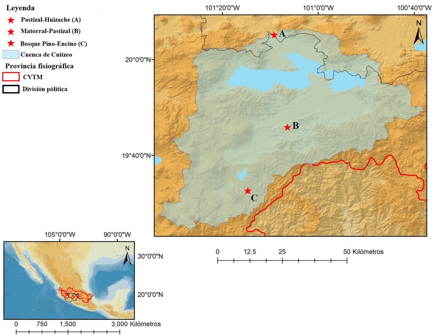
La caracterización de la vegetación se hizo en el estrato herbáceo mediante 5 cuadrantes de 5 m², cada cuadrante con 5 unidades de muestreo de 1 m² (25 unidades en total, por cada sitio y para cada estación), distribuidas en arreglo “5 de oros”, una en el centro y las demás en las esquinas (Senasica, 2024). Se identificaron familias y géneros, y se registró su abundancia y cobertura horizontal en porcentaje. La determinación taxonómica de las plantas se limitó a género debido al estado fenológico de las plantas en algunas estaciones, se utilizó el término morfotipo para las plantas solo identificadas hasta familia.
Para la vegetación se describió la estructura general en los niveles taxonómicos de familia y género para cada sitio y época del año incluyendo composición y abundancias.
Para los roedores se analizó la riqueza y abundancia para cada localidad, época de recolecta y para todo el año. Para evaluar la relación entre la riqueza de especies en función del esfuerzo de muestreo, se elaboraron curvas de rarefacción para cada sitio que permitieron estimar la eficiencia del muestreo utilizando el acumulado por individuos (Chao et al., 2014, 2016). Posteriormente, se estimó la completitud del muestreo a través de las estimaciones no paramétricas de riqueza de Chao 2 y bootstrap. Se elaboraron curvas de rango-abundancia para describir las relaciones de abundancia entre las especies y determinar las dominancias para cada localidad y época del año.
Se calcularon los índices de diversidad de Shannon-Wiener (H´) y dominancia Simpson (D), tanto por sitio de estudio como por temporada. Se utilizó la prueba de t modificada por Hutchenson (1970) para probar las diferencias estadísticas, se incluyó además el cálculo de los límites de confianza (LC) a 95% por el método de percentiles. Para calcular la equitatividad de las especies se usó el índice de equitatividad de Pielou (J). Para conocer el grado de semejanza entre comunidades se usó el índice de similitud de Jaccard para composición de especies y el índice de Bray-Curtis para considerar la abundancia en la comparación (Magurran, 2004).
Con el fin de evaluar posibles diferencias en la composición de especies en relación con los hábitats, se aplicó un análisis de las similitudes entre comunidades (Anosim), con 10,000 permutaciones y disimilitud de Bray-Curtis. Todos los análisis antes mencionados se hicieron con el Software Past 4.12 (Hamer et al., 2001).
Resultados
La comunidad vegetal durante un ciclo anual se caracterizó por presentar 31 familias y 105 géneros de plantas en una muestra de 15,060 individuos del estrato herbáceo, de los que 51% correspondió a la asociación pastizal-huizache. El 39% se registró para matorral-pastizal y 10% en pino-encino.
En la asociación pastizal-huizache predominó la familia Poaceae, con abundancia relativa (AR) de 80% y cobertura horizontal relativa (CH) de 86%. Destacan los géneros Chloris (AR = 44%; CH = 51%), Paspalum (AR = 12%; CH = 3%) y Distichlis (AR = 9%; CH = 22%), esas proporciones fueron constantes durante todo el año. En el estrato arbóreo destaca el huizache (Vachellia sp.).
Tabla 1
Especies registradas y sus abundancias (absoluta y relativa = tasas de captura) en 3 asociaciones vegetales de la cuenca de Cuitzeo en un ciclo de muestreo anual. S = Secas; H = húmedas; PLL = posterior a lluvias; SF = secas frías.
| Especie | Pastizal-huizache (1,838 m snm) | Matorral-pastizal (1,896 m snm) | Pino-encino (2,132 m snm) | Subtotales (tasa de captura) | |||||||||
| Heteromys irroratus | 0 | 2 | 0 | 0 | 0 | 1 | 0 | 7 | 0 | 0 | 0 | 0 | 10 (0.31) |
| Baiomys taylori | 0 | 1 | 0 | 3 | 1 | 1 | 3 | 28 | 0 | 0 | 0 | 0 | 37 (1.16) |
| Baiomys musculus | 1 | 0 | 0 | 0 | 1 | 0 | 0 | 0 | 0 | 0 | 0 | 0 | 2 (0.063) |
| Sigmodon hispidus | 0 | 0 | 0 | 2 | 0 | 0 | 0 | 0 | 0 | 0 | 0 | 0 | 2 (0.063) |
| Sigmodon mascotensis | 0 | 0 | 0 | 1 | 0 | 0 | 0 | 0 | 0 | 0 | 0 | 0 | 1(0.031) |
| Oligoryzomys fulvescens | 0 | 1 | 0 | 0 | 0 | 0 | 0 | 0 | 1 | 0 | 0 | 0 | 2 (0.063) |
| Peromyscus labecula | 0 | 0 | 0 | 0 | 0 | 0 | 0 | 0 | 0 | 0 | 1 | 0 | 1(0.031) |
| Peromyscus melanotis | 0 | 0 | 0 | 0 | 0 | 0 | 0 | 0 | 0 | 0 | 0 | 1 | 1(0.031) |
| Peromyscus difficilis | 0 | 1 | 0 | 0 | 0 | 0 | 0 | 1 | 0 | 1 | 4 | 5 | 12 (0.37) |
| Peromyscus hylocetes | 0 | 0 | 0 | 1 | 0 | 0 | 0 | 0 | 0 | 0 | 0 | 1 | 2 (0.063) |
| Peromyscus kilpatricki | 0 | 0 | 0 | 1 | 0 | 0 | 0 | 0 | 0 | 0 | 0 | 3 | 4 (0.12) |
| Peromyscus pectoralis | 0 | 2 | 0 | 0 | 0 | 0 | 0 | 0 | 0 | 0 | 0 | 0 | 2 (0.063) |
| Peromyscus gratus | 0 | 0 | 0 | 0 | 0 | 0 | 0 | 0 | 0 | 0 | 3 | 1 | 4 (0.12) |
| Peromyscus zamorae | 0 | 0 | 0 | 0 | 0 | 0 | 0 | 0 | 0 | 0 | 2 | 0 | 2 (0.063) |
| Reithrodontomys sumichrasti | 0 | 0 | 0 | 0 | 0 | 0 | 0 | 0 | 1 | 0 | 0 | 5 | 6 (0.18) |
| Reithrodontomys fulvescens | 0 | 0 | 0 | 0 | 0 | 0 | 0 | 1 | 0 | 0 | 1 | 0 | 2 (0.063) |
| Mus musculus | 0 | 3 | 1 | 1 | 2 | 0 | 1 | 0 | 0 | 0 | 0 | 0 | 8 (0.25) |
| Submuestra por sitio (%) | 21 (21.4) | 47 (47.9) | 30 (30.6) | 98 (100%) | |||||||||
| Riqueza de especies por sitio | 11 | 6 | 10 | 17 | |||||||||
| Tasa de captura/área | 1.98 | 4.45 | 2.84 | 3.09 | |||||||||
| Especies exclusivas por sitio | 3 | 0 | 5 | 8 |
Tabla 2
Parámetros de riqueza, abundancia (en paréntesis) y tasa de captura de la comunidad de roedores en 3 asociaciones vegetales en función a la época.
| Secas | Húmedas | Posterior a lluvias | Secas frías | |
| Pastizal-huizache | 1-(1)-0.56 | 6-(10)-4.1 | 1-(1)-0.3 | 6-(9)-2.5 |
| Matorral-pastizal | 3-(4)-2.2 | 2-(2)-0.83 | 2-(4)-1.4 | 4-(37)-10.4 |
| Pino-encino | 2-(2)-1.1 | 1-(1)-0.42 | 5-(11)-3.9 | 6-(16)-4.5 |
| Esfuerzo de muestreo/trampas-noche | 540 | 720 | 840 | 1,068 |
| Especies | 5 | 6 | 7 | 12 |
| Especies exclusivas | 1 | 1 | 2 | 6 |
| Sub muestra estacional (%) | 7 (7.1) | 13 (13.2) | 16 (16.3) | 62 (63.2) |
| Tasas de captura general/estación | 1.30 | 1.81 | 1.90 | 5.81 |
El matorral-pastizal está integrado proporcionalmente por las familias Asteraceae (18%), Poaceae (16%), Fabaceae (14%) y Euphorbiaceae (11%). Difiere del pastizal al presentar variación estacional en la estructura y composición de las plantas en el año. Por ejemplo, en secas Lolium presentó la mayor abundancia y cobertura horizontal (AR = 43%; CH = 32%); en temporada húmeda Marina (AR = 29%; CH = 21%), Euphorbia (AR = 22%; CH = 13%) y Adenophyllum (AR = 20%; CH = 19%); en la temporada posterior a lluvias Simsia (AR = 20%; CH = 20%) y Eragrostis (AR = 16%; CH = 16%), y en secas frías, una especie de gramínea (AR = 42%; CH = 55%), que por su fenología no pudo ser identificada. También se presentaron elementos aislados de Opuntia.
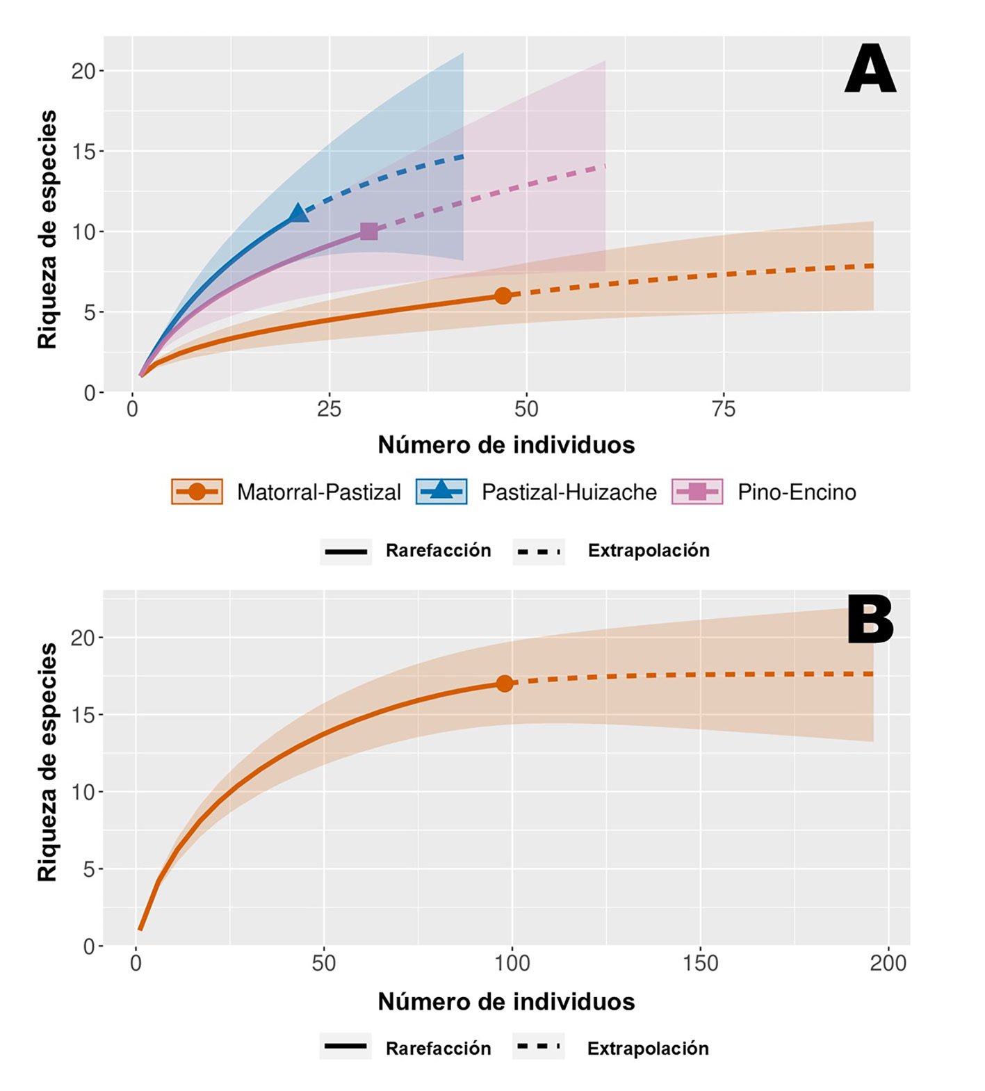
Figura 2. A, Curvas de rarefacción de riqueza de especies en función de las abundancias de roedores en sitios de colecta; B, curva de rarefacción con riqueza de especies en función abundancias de roedores colectadas durante el ciclo anual en los 3 sitios.
La vegetación en el área de pino-encino se caracterizó en el estrato arbóreo por la presencia de Pinus y Quercus. El estrato herbáceo se caracterizó por el predominio de las familias Poaceae, Rosaceae, Asteraceae, Oxiladaceae, Fabaceae, Anacardiaceae, Pteridaceae y Cyperaceae con 78% de la muestra total. El género Rubus (AR = 29%; CH = 13%) predominó en secas, mientras que en húmedas fue Oxalis (AR = 31%; CH = 9%) y Centella (AR = 19%; CH = 17%); en la temporada post-lluvias (AR = 19%; CH = 11%) y secas frías (AR = 27%; CH = 13%) fueron macollos de gramíneas que carecían de espiga por lo que no se identificaron, posiblemente del género Microstegium (apéndice 1).
La muestra de roedores capturados incluyó 98 individuos. Los ejemplares se identificaron como 16 especies nativas y Mus musculus (introducida), pertenecientes a 7 géneros en las familias Cricetidae (15), Heteromyidae (1) y Muridae (1) (tabla 1).
Con base en la curva de rarefacción, se interpreta el esfuerzo de muestreo como suficiente en registrar la riqueza esperada de los 3 sitios; con una cobertura de la muestra de 93% en matorral-pastizal, 83% en el bosque de pino-encino y 72% en pastizal-huizache (fig. 2A). A nivel regional, según los estimadores Chao 2 y bootstrap, la riqueza se espera entre 18-19 especies, solo 2 por encima de la riqueza observada, lo que permite asumir un muestreo de inventario de especies de roedores para la zona suficientemente completo, y que se corrobora con una cobertura de muestra total de 97% en la curva de rarefacción (fig. 2B). Siendo en el pastizal-huizache y en el bosque de pino-encino donde existe mayor oportunidad de registrar otras especies.
La mayor riqueza de especies se observó en el pastizal-huizache, seguido de la asociación de pino-encino y la asociación matorral-pastizal, y en este mismo orden las abundancias se comportaron de menor a mayor (tabla 1; fig. 3A). En relación con la temporada de recolecta, la riqueza y abundancia en secas es en la que se obtuvo la menor cantidad de ejemplares. Posteriormente, se incrementó el éxito de captura para las temporadas siguientes hasta llegar a secas frías (tabla 2); sumando los datos de riqueza y abundancia de las 3 comunidades se observa un incremento en la complejidad (fig. 3B). En las temporadas invernales (secas frías) se destaca la mayor abundancia y tasas de captura de todo el estudio, particularmente en el matorral-pastizal. También se registró la mayor riqueza de especies (n = 12), la mayor abundancia absoluta (62 individuos) y la mayor tasa de captura de 5.8/100 trampas-noche (tabla 2).
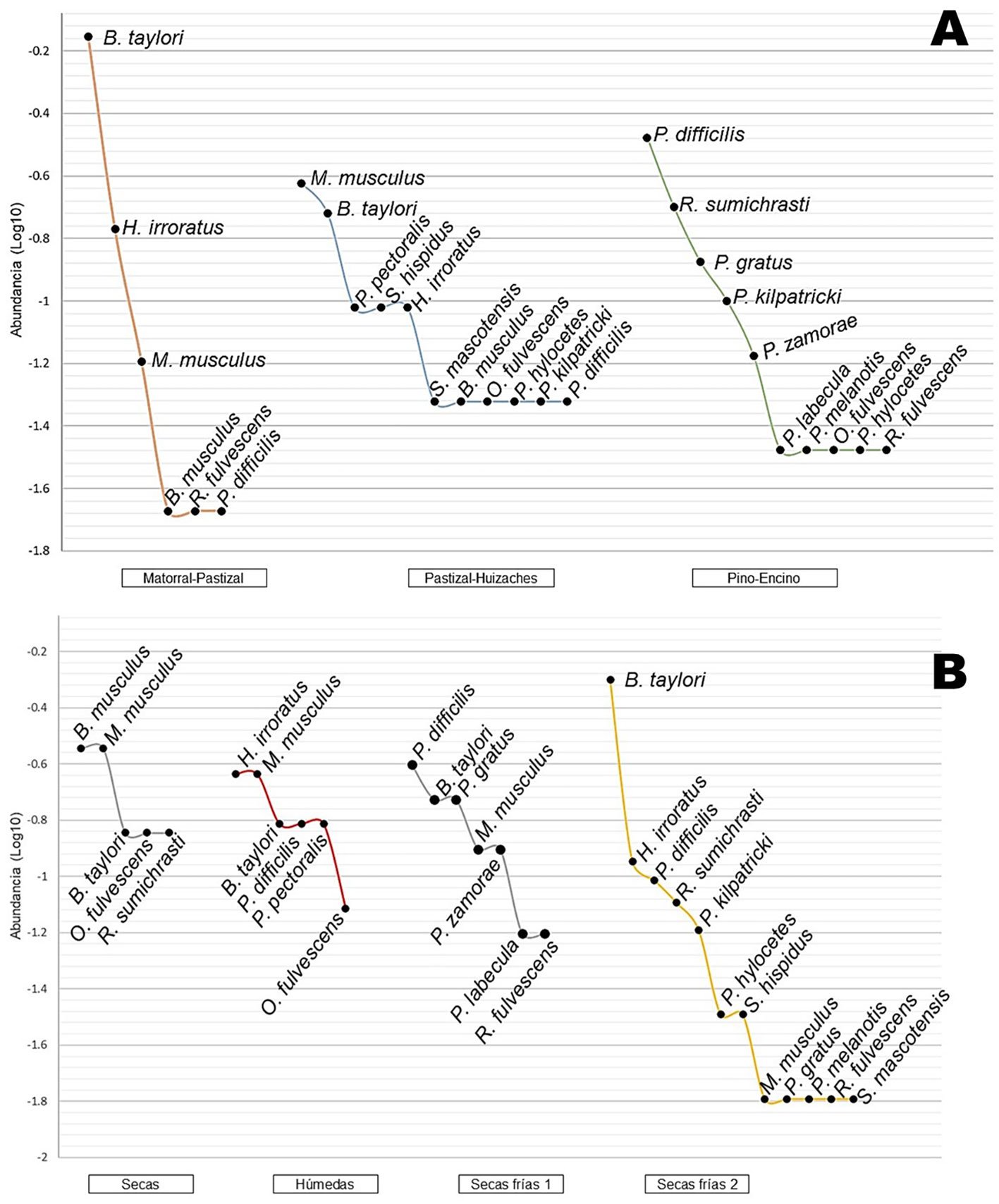
Figura 3. A, Curvas de rango-abundancia entre los sitios de estudio; B, curvas de rango-abundancia entre las temporadas del año de estudio sumando los 3 hábitats.
Baiomys taylori fue la especie más abundante, representó 33% del total de individuos recolectados, con los valores más altos en la temporada de secas frías, se presentó durante todo el año principalmente en matorral-pastizal (n = 33), seguido de pastizal-huizache (n = 4). La especie que resultó con mayor abundancia en el hábitat de pastizal-huizache fue Mus musculus, que también se registró en matorral-pastizal y presente durante todo el año. Para el bosque de pino-encino las especies con más individuos fueron Peromyscus difficilis y Reithrodontomys sumichrasti, la primera se encontró todo el año exceptuando en secas, además destaca por ser la única registrada para las 3 localidades. Por el contrario, las especies Peromyscus labecula, Peromyscus melanotis, y Sigmodon mascotensis, estuvieron representadas por solo 1 individuo; mientras que Baiomys musculus, Oligoryzomys fulvescens, Peromyscus hylocetes, Peromyscus zamorae, Peromyscus pectoralis, Reithrodontomys fulvescens y Sigmodon hispidus contaron con 2 ejemplares, estas especies en conjunto representan 59% de la riqueza total del estudio (fig. 3; tabla 1).
Tabla 3
Valores con el índice de diversidad de Shannon-Wiener (H´), índice dominancia de Simpson (D) e índice de equidad de Pielou (J) para la comunidad de roedores de la cuenca de Cuitzeo. Prueba de t modificada por Hutchenson H´/D para diferencias significativas (*).
| Prueba de t modificada por Hutchenson | ||||||
| H´ | D | J | Matorral-pastizal | Pastizal-huizache | Pino-encino | |
| Matorral-pastizal | 0.97 | 0.52 | 0.54 | D = 3.8822E-05* | D = 0.00042* | |
| Pastizal-huizache | 2.19 | 0.13 | 0.91 | H´ = 3.035E-06* | D = 0.3657 | |
| Pino-encino | 1.93 | 0.18 | 0.84 | H´ = 6.886E-05* | H´ = 0.276 |
Mediante el índice de diversidad de Shannon-Wiener (H´) y la equitatividad de Pielou (J), con límites de confianza (LC) de 95%, se concluye que el hábitat que presentó mayor diversidad y equitatividad en la comunidad de pequeños roedores fue el pastizal-huizache con H´ = 2.19 (LC = 1.69-2.29) y J = 0.91 (LC = 0.81-0.96), en cambio matorral-pastizal fue poco diverso con H´ = 0.97 (LC = 0.66-1.22) y su equitatividad fue las más baja con J = 0.54 (LC = 0.42-0.70); el bosque de pino-encino presento una diversidad de H´ = 1.93 (LC = 1.68-2.13) y J = 0.84 (LC = 0.74-0.92). La prueba de t modificada por Hutchenson no muestra diferencias significativas entre pastizal-huizache y pino-encino, pero sí entre matorral-pastizal con respecto a las otras 2 comunidades. Este efecto también se observa con el cálculo de los límites de confianza en donde solamente en pastizal-huizache y pino-encino existe traslape tanto en H´ como en J. En relación con la temporada de recolecta y como se observa en la tabla 1, en algunos casos solo se capturaron 1 o 2 ejemplares por sitio y temporada, por tanto, conocer la diversidad de los sitios en función de las temporadas no es posible. Aun así, si se toma la sumatoria de los 3 hábitats por época de recolecta se observa poca variación de la diversidad: secas, H´ = 1.55 (LC = 0.79-1.55); húmedas H´ = 1.73 (LC = 1.26-1.73); post lluvias, H´ = 1.84 (LC = 1.35-1.87) y finalmente secas frías, H´ = 1.75 (LC = 1.41-1.99), sin diferencias significativas entre temporadas del año y traslape de los intervalos de confianza en todos los casos.
Por su parte, con el índice de dominancia de Simpson (D) el valor más alto se registró en matorral-pastizal con D = 0.52 y su dominancia con la especie B. taylori es diferente a los otros 2 sitios, en donde no se observaron especies dominantes (tabla 3).
De acuerdo con el índice de similitud de Jaccard para la composición de la comunidad de roedores, el matorral-pastizal y pastizal-huizaches presentan mayor similitud, a diferencia de la comparación entre matorral-pastizal y bosque pino-encino con menor similitud; considerando las abundancias, este patrón se repite según el índice de Bray-Curtis (tabla 4). Con el análisis de similitud entre comunidades (Anosim) se estima diferencias significativas (R = 0.35; p = 0.008) en la composición y abundancia entre los hábitats matorral-pastizal y bosque de pino-encino (p = 0.030) (fig. 4).
Tabla 4
Índice de similitud de Jaccard (ISJ) y Bray-Curtis (BC) para la comunidad de roedores en las 3 asociaciones vegetales examinadas de la cuenca de Cuitzeo.
| Matorral-pastizal | Pastizal-huizache | Pino-encino | |
| Matorral-pastizal | 1 | BC = 0.32 | BC = 0.05 |
| Pastizal-huizache | ISJ = 0.41 | 1 | BC = 0.15 |
| Pino-encino | ISJ = 0.14 | ISJ = 0.23 | 1 |
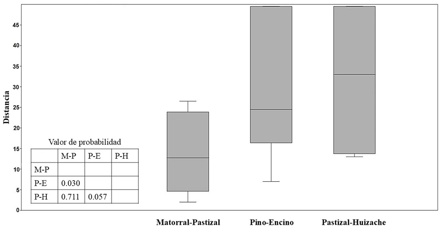
Figura 4. Boxplot y valores de probabilidad del análisis de similitudes (Anosim) entre las 3 asociaciones vegetales para la comunidad de roedores en de la cuenca de Cuitzeo (R = 0.35; p = 0.008). M-P = Matorral-pastizal, P-E = bosque de pino-encino y P-H = pastizal-huizache.
Discusión
Los resultados obtenidos ofrecen 4 aspectos emergentes: riqueza de especies, baja abundancia general, mayores abundancias invernales y baja similitud relativa entre los ambientes muestreados. Recientemente, se evaluó la mastofauna que habita en la cuenca de Cuitzeo. En total se registraron 68 especies de mamíferos, con 28 del orden Rodentia, que representaron 54% de las especies registradas en Michoacán (Monterrubio et al., 2019). Con el presente trabajo se suman al registro de Rodentia para la región a B. musculus, P. pectoralis y O. fulvescens, especies que están presentes en otras áreas del eje Neovolcánico y el bajío (Sánchez et al., 2005), pero que no habían sido registradas para la cuenca. Al incluir estos nuevos registros para la cuenca, en esta zona se presenta 60% de las especies de roedores documentadas para Michoacán (Monterrubio et al., 2014). Otro aspecto notable, es que el esfuerzo de muestreo desarrollado proporcionó el registro del mayor número de especies (16) en cualquier estudio efectuado para la cuenca (Apéndice 2). Esta riqueza sobresale también en el contexto nacional, ya que los intervalos de riqueza específica reportados suelen estar entre 5 y 18 especies (Apéndice 3), generalmente se observan valores bajos en áreas pequeñas y aumentan cuando el estudio es a escala regional.
En contraste, fue sorpresiva la baja abundancia general, con solo 98 registros, en comparación con otros estudios de diferentes regiones del país, en los que con esfuerzos entre 455 y 28,242 noches/trampa se obtienen capturas superiores a 100 individuos (Apéndice 3). Una razón probable de la baja abundancia para la mayoría de especies puede ser la disminución de las precipitaciones en la región. Con base en los datos históricos y comparando con los últimos años, se ha experimentado sequía en algunas partes de la cuenca (Hernández et al., 2023), para lo que probablemente hayan respondido las poblaciones de roedores con menor reproducción o migración. Otra evidencia es la cifra de capturas del muestreo de la temporada de secas frías (fig. 3B) y posterior a la época de lluvia de la cuenca, dado que se registró un incremento notable en el número de capturas, tanto en riqueza específica como en abundancia. Este fenómeno es similar al observado en otros estudios (Flores y Vázquez, 2016; Zaragoza et al., 2022). El aumento poblacional en esta época ocurrió para B. taylori, P. difficilis y H. irroratus; en las primeras 2 especies ya se ha registrado aumento en densidades poblacionales en temporadas frías del año (Eshelman y Cameron, 1987; Fernández et al., 2010), mientras que el aumento de H. irroratus, según antecedentes, se reporta de agosto a noviembre (Dowler y Genoways, 1978).
El índice de diversidad no muestra variación significativa entre épocas del año, esto podría indicar que la diversidad es explicada en mayor medida por el hábitat y que genera niveles importantes de estabilidad reflejada en los valores de equitatividad obtenidos (entre 0.57 y 1), lo cual también sugieren Luévano et al. (2008), particularmente en zonas de matorrales.
Las 3 comunidades de roedores examinadas muestran en general baja similitud, y parece observarse una posible influencia de la estratificación de la vegetación. En general, a mayor complejidad estructural de la vegetación con presencia del estrato arbóreo, se observa mayor riqueza de especies. Este patrón se presentó para el pastizal-huizache y el bosque de pino-encino en donde no existió diferencia significativa de diversidad y tampoco hubo traslape de intervalos de confianza. En cambio, la abundancia de roedores fue mayor en el matorral-pastizal y en el pino-encino, en ambos hábitats se observa mayor riqueza de la vegetación a nivel herbáceo. El patrón de aumento en las abundancias para ambientes de mayor heterogeneidad también lo encontraron Morales et al. (2019) y contrasta con la homogeneidad del estrato herbáceo y baja densidad de roedores registrada para el pastizal-huizache de este estudio. Todavía no es clara la relación entre la estructura de la comunidad de roedores y la conectividad de los hábitats. La dinámica de la cuenca de Cuitzeo implica un aumento de la colonización humana y más actividades agropecuarias en las últimas décadas (Escamilla y Aguilar, 2010). Dicha expansión ha degradado y fragmentado los hábitats originarios, hasta llegar a tener 6% con asentamientos humanos y 50% de la cuenca destinado a zonas de cultivo y pastoreo (INEGI, 2023). Con este panorama, es posible que la estructura y composición de las comunidades de pequeños roedores observada puede deberse al grado de aislamiento diferenciado entre los distintos hábitats. Los pastizales presentan conectividad con los extensos cultivos, permitiendo la cohesión espacial de algunas especies, mientras que las zonas de matorral y arbóreas presentan índices muy bajos de conectividad (Correa et al., 2014). El aislamiento en estos hábitats, principalmente matorrales, puede disminuir a los depredadores, lo que se ve reflejado en el aumento de poblaciones de roedores más generalistas y menor riqueza especifica (Young et al., 2015); este proceso puede estar presente en el sitio de matorral-pastizal. Aunque en el caso de las zonas montañosas de la cuenca con bosques, todavía parece existir mayor conectividad y esta se ve reflejada en la riqueza de la mastofauna (Monterrubio et al., 2019).
El pastizal-huizache se extendía originalmente en forma extensa (López et al., 2010), ahora es un ambiente con elevada fragmentación y es quizás uno de los hábitats más amenazados por el elevado establecimiento de asentamientos humanos y campos de cultivo. Sin embargo, la diversidad de roedores observada en este hábitat parece todavía estar explicada por la vegetación más que por la antropización vecina. Los 3 géneros de plantas herbáceas más representativos de la zona (Chloris, Distichlis y Panicum) son gramíneas no invasivas y componentes de la vegetación original (Herrera y Pámanes, 2010). Peromyscus pectoralis, Sigmodon hispidus y S. mascotensis resultaron exclusivas a esta localidad entre los 3 hábitats estudiados, y parecen coincidir con ambientes en que se han registrado regularmente, que incluyen aridez relativa, pastizales y ambientes rocosos (Baccus et al., 2009; Fleharty y Olson, 1969; Martínez et al., 2017). En hábitats similares la exclusividad reportada suele ser de 1 a 2 especies (Cimé et al., 2010; Elizalde et al., 2014; Hernández et al., 2012), lo cual coincide con lo registrado en este trabajo. Además, la cercanía con sembradíos parece proveer de alimento, lo que facilita la coexistencia entre especies, ya que los roedores también consumen materiales de los cultivos, como se ha documentado en plantaciones de caña (Peña et al., 2009).
Para el matorral-pastizal, la baja diversidad de roedores podría explicarse en parte por la poca conectividad y por la biología de la comunidad vegetal, ya que los géneros más abundantes están asociados con ambientes alterados. En temporada seca el género herbáceo Lolium (Poaceae), especie introducida en México (Herrera y Pámanes, 2010), fue la más abundante y fue en esta temporada cuando se recolectaron pocos roedores (n = 4), 2 de los cuales fueron M. musculus, especie que puede considerarse indicadora de deterioro del hábitat. En relación con las plantas de temporadas restantes del año, son géneros nativos con distribución principalmente en matorrales como Marina (M. cf. nutans) y Adenophyllum, y junto con Euphorbia (E. cf. dentata), Simsia (S. cf. foetida) y Eragrostis (E. cf. intermedia), pero crecen en afinidad a lugares ruderales con tendencia a disturbios (Rzedowski y Rzedowski, 2005). En los recorridos de campo se observaron asentamientos humanos e infraestructura inconclusa, indicativa de la expansión de la mancha urbana, así como fauna doméstica, perros principalmente, caminando en búsqueda de alimento entre la vegetación.
El registro de B. taylori, especie que se conoce con una mayor densidad de individuos distribuyéndose en matorrales y zonas áridas (Packard, 1960), coincidió con el hábitat de recolecta. Este cricétido junto con H. irroratus podrían ilustrar su resiliencia a los ambientes perturbados, tendencia que se ha reportado para mamíferos de tallas pequeñas, particularmente en roedores y murciélagos (Dirzo et al., 2014), aunque también pudiesen ser evidencia de que el hábitat de matorral-pastizal en la región experimenta un proceso de homogeneización de la comunidad de roedores.
Por su parte, el bosque de pino-encino (La Planta) solo se diferencia con el pastizal-huizache por tener una especie menos (la invasora M. musculus); pero en índices cuantitativos la similitud fue baja. Este hábitat, donde cobertura y dominancia de biomasa vegetal corresponden a Pinus y Quercus (Gómez-Tagle et al., 2015), no se recolectaron especies de roedores introducidas. O. fulvescens, R. sumichrasti y las especies del género Peromyscus se reportan en bosques conservados y áreas con corrientes de agua cercanas (Fernández et al., 2010; Spencer y Cameron, 1982), lo cual coincide en lo general con este estudio. Sin embargo, aunque parece un espacio conservado por la estructura de su comunidad de roedores y su flora, también presenta cambio en el uso de suelo en los alrededores, principalmente por expansión del cultivo del aguacate y arándano. Aquí se presentaron 5 especies exclusivas, y coincide con lo registrado en otros estudios en ambientes semejantes en los que la exclusividad de especies va de 1-4 (Flores y Vázquez, 2016; Mendoza y Horváth, 2013; Villanueva, et al., 2017; Zalapa et al., 2012).
Es importante continuar con muestreos con el fin de conocer mejor la dinámica estacional y espacial de las poblaciones de roedores en los distintos ambientes, ya que cada hábitat difiere de nivel de fragmentación y extensión en la cuenca, sobre todo en esta región considerada de importancia para la conservación de la biodiversidad en todos los niveles (Aguilar et al., 2010). Finalmente, en el centro de México desaparecen rápidamente los hábitats naturales, es urgente utilizar la información generada por múltiples inventarios para la priorización y establecimiento de áreas a restaurar y para conservar espacios representativos de todos los hábitats, especialmente donde habitan especies endémicas como lo es Peromyscus ensinki (Bradley et al., 2021). En la cuenca debe estudiarse el grado de tolerancia que especies listadas en categorías de riesgo tienen a la perturbación y como coexisten con especies introducidas, anticipando y examinando los riesgos potenciales de enfermedades zoonóticas, sin olvidar que el bienestar económico no puede lograrse en un entorno sin servicios ambientales y biodiversidad (Villafán et al., 2021; Young et al., 2014).
Referencias
Aguilar, V., Kolb, M., Koleff, P. y Urquiza-Haas, T. (2010). Las cuencas de México y su biodiversidad: una visión integral de las prioridades de conservación. En H. Cotler, A. Garrido, N. Luna, C. Enríquez y M. L. Cuevas (Eds.), Las cuencas hidrográficas de México. Diagnóstico y priorización (pp. 142–151). Ciudad de México: Instituto Nacional de Ecología.
Aragón, E. E., Garza, A. y Cervantes, F. A. (2009). Estructura y organización de los ensambles de roedores de un bosque de la Sierra Madre Occidental, Durango, México. Revista Chilena de Historia Natural, 82, 523–542. http://dx.doi.org/10.4067/S0716-078X2009000400007
Baccus, J. T., Hardwick, J. M., Huffman, D. G. y Kainer, M. A. (2009). Seasonal trophic ecology of the white-ankled mouse, Peromyscus pectoralis (Rodentia: Muridae) in central Texas. Texas Journal of Science, 61, 97–118.
Barragán, F., Lorenzo, C., Morón, A., Briones, M. A. y López, S. (2010). Bat and rodent diversity in a fragmented landscape on the Isthmus of Tehuantepec, Oaxaca, México. Tropical Conservation Science, 3, 1–16. https://doi.org/10.
1177/194008291000300101
Bradley, R. D., Francis, J. Q., Platt, R. N., Soniat, T. J., Álvarez, D. y Lindsey, L. L. (2019). Mitochondrial DNA sequence data indicate evidence for multiple species within Peromyscus maniculatus. Lubbock, TX: Museum of Texas Tech University.
Bradley, R. D., Ordóñez, N., Ceballos, G., Rogers, D. S. y Schmidly, D. J. (2017). A new species in the Peromyscus boylii species group (Cricetidae: Neotominae) from Michoacán, México. Journal of Mammalogy, 98, 154–165. https://doi.org/10.1093/jmammal/gyw160
Bradley, R. D., Ordóñez, N., Thompson, C. W., Wright, E. A., Ceballos, G., Kilpatrick, C. W. et al. (2021). Two new species of Peromyscus (Cricetidae: Neotominae) from the Transverse Volcanic Belt of México. Journal of Mammalogy, 103, 255–274. https://doi.org/10.1093/jmammal/gyab128
Bravo-Espinosa, M., García-Oliva, F., Ríos-Patrón, E., Mendoza-Cantú, M. E., Barrera-Camacho, G., López-Granados, E. et al. (2008). La cuenca del lago de Cuitzeo: problemática, perspectivas y retos hacia su desarrollo sostenible. Morelia Michoacán, México: Consejo Estatal de Ciencia y Tecnología de Michoacán (COECYT). https://doi.org/10.22201/ciga.9789707035782p.2008
Carlón, T. y Mendoza, M. (2007). Análisis hidrometeorológico de las estaciones de la cuenca del lago de Cuitzeo. Investigaciones Geográficas, Boletín del Instituto de Geografía, UNAM, 63, 56–76. https://doi.org/10.14350/rig.29910
Castro, A., Salame, A., Vergara, J., Castillo, A. y Ramírez, J. (2008). Fluctuaciones de micromamíferos terrestres en bosques templados aledaños a la Ciudad de México, Distrito Federal. En C. Lorenzo, E. Espinoza y J. Ortega (Eds.), Avances en el estudio de los mamíferos de México II (pp. 391–410). San Cristóbal de las Casas, Chiapas: Asociación Mexicana de Mastozoología.
Ceballos, G. y Oliva, G. (2005). Los mamíferos silvestres de México. México D.F.: Conabio/ Fondo de Cultura Económica.
Chao, A., Gotelli, N. J., Hsieh, T. C., Sander, E. L., Ma, K. H., Colwell, R. K. et al. (2014). Rarefaction and extrapolation with Hill numbers: a framework for sampling and estimation in species diversity studies. Ecological Monographs, 84, 45–67. https://doi.org/10.1890/13-0133.1al/gyw160
Chao, A., Ma, K. H. y Hsieh, T. C. (2016) iNEXT (iNterpolation and EXTrapolation) Online: Software for interpolation and extrapolation of species diversity. Program and user’s guide. http://chao.stat.nthu.edu.tw/wordpress/software_download/inext-online/
Cimé, J. A., Hernández, S. F., Barrientos, R. C. y Castro, A. A. (2010). Diversidad de pequeños roedores en una selva baja caducifolia del noreste de Yucatán, México. Therya, 1, 23–39. https://doi.org/10.12933/therya-10-2
Correa, C. A., Mendoza, M. E. y López, E. (2014). Análisis del cambio en la conectividad estructural del paisaje (1975-2008) de la cuenca de Cuitzeo, Michoacán, México. Revista de Geografía Norte Grande, 59, 7–23. http://dx.doi.org/10.4067/S0718-34022014000300002
Dirzo, R., Young, H. S., Galetti, M., Ceballos, G., Isaac, N. J. B. y Collen, B. (2014). Defaunation in the Anthropocene. Science, 345, 401–406. https://www.science.org/doi/10.1126/science.1251817
Dowler, R. C. y Genoways, H. H. (1978). Liomys irroratus. Mammalian Species, 82, 1–6. https://doi.org/10.2307/3503813
Elizalde, C., López, J. C., Hernández, L., Laundré, J. W., Cervantes, F. A., Morales-Mejía, F. M. et al. (2014). Registro de presencia y actividades de algunos mamíferos en el Desierto Chihuahuense, México. Therya, 5, 793–816. https://doi.org/10.12933/therya-14-252
Escamilla, I. y Aguilar, G. (2010). Urbanización. En S. Cram, L. Galicia, I. Israde, C. López y B. Ávila (Eds.), Atlas de la cuenca del lago de Cuitzeo: análisis de su geografía y entorno socioambiental (pp. 160–163). México D.F.: UNAM/ UMSNH.
Eshelman, B. D. y Cameron, G. N. (1987). Baiomys taylori. Mammalian Species, 285, 1–7. https://doi.org/10.2307/3503776
Fernández, J. A., García-Campusano, F. y Hafner, M. S. (2010). Peromyscus difficilis (Rodentia: Cricetidae). Mammalian Species, 42, 220–229. https://doi.org/10.1644/867.1
Fleharty, E. D. y Olson, L. E. (1969). Summer food habits of Microtus ochrogaster and Sigmodon hispidus. Journal of Mammalogy, 50, 475–486. https://doi.org/10.2307/1378774
Flores, R. y Vázquez, G. (2016). Influence of vegetation type and season on rodent assemblage in a mexican temperate forest mosaic. Therya, 7, 357–369. https://doi.org/10.12933/therya-16-390
García, U. O. y Flores, O. A. (2010). Biodiversidad: anfibios y reptiles. En S. Cram, L. Galicia, I. Israde, C. López y B. Ávila (Eds.), Atlas de la cuenca del lago de Cuitzeo: análisis de su geografía y entorno socioambiental (pp. 94–95). México D.F.: UNAM/ UMSNH.
García, C., Romero, M. L. y Sánchez C. (2002). Comparison of rodent communities in sites with different degrees of disturbance in deciduous forest of southeastern Morelos, México. Acta Zoológica Mexicana, 85, 153–168. https://doi.org/10.21829/azm.2002.85851819
Gloria-Tapia, G., López, C., González, A. y Hernández, S. F. (2012). Diversidad de roedores y su relación con la heterogeneidad ambiental en la cuenca del río Nazas, Durango, México. En F. A. Cervantes y C. Ballesteros (Eds.), Estudio sobre la biología de roedores silvestres mexicanos (pp. 59–70). México D.F.: Instituto de Biología, UNAM.
Godinez, E. y Guerrero, S. (2014). Los roedores de Jalisco, México: clave de determinación. Therya, 5, 633–678. https://doi.org/10.12933/therya-14-212
Gómez-Tagle, A., Gómez-Tagle, A. F., Ávila, J. A. y Bruijnzeel, L. (2015). Partición de la precipitación en un bosque tropical montano de pino-encino en el centro de México. Bosque, 36, 505–518. https://doi.org/10.4067/S0717-92002015000300017
González, A., Rodríguez, N. V. y Marín, G. (2012). Composición del ensamble de pequeños mamíferos del borde de un bosque mesófilo de montaña en Veracruz, México. En F. A. Cervantes y C. Ballesteros (Eds.), Estudio sobre la biología de roedores silvestres mexicanos (pp. 85–96). México D.F.: Instituto de Biología, UNAM.
Hamer, Q., Harper, D. A. T. y Ryan, P. D. (2001). PasT: Paleontological Statistics Software Package for Education and Data Analysis. Paleontologia Electronica, 4, 1–9.
Hernández, S. F., Cimé, J. A., Medina, S. y Durán C. M. (2012). Parámetros poblacionales del ratón yucateco Peromyscus yucatanicus de una selva baja caducifolia del norte de Yucatán, México. En F. A. Cervantes y C. Ballesteros. (Eds.), Estudio sobre la biología de roedores silvestres mexicanos (pp. 151–164). México D.F.: Instituto de Biología, UNAM
Hernández, L., Laundré, J. W., González, A., López, J. y Grajales, K. M. (2011). Tale of two metrics: density and biomass in a desert rodent community. Journal of Mammalogy, 94, 840–851. https://doi.org/10.1644/10-MAMM-A-175.1
Hernández, A., Ortiz, C. F. y Alcaraz, J. V. (2023). El riesgo agrícola ante el cambio climático en la región de Cuitzeo del estado de Michoacán, México. Acta Universitaria Multidisciplinary Scientific Journal, 33, 1–19. https://doi.org/10.15174/au.2023.3763
Herrera, Y. y Pámanes, D. S. (2010). Guía de pastos de Zacatecas. Durango, Durango, México: IPN/ Conabio.
Hutchenson, K. (1970). A test for comparing diversities base on the Shannon formula. Journal of Theoretical Biology, 29, 151–154.
INEGI (Instituto Nacional de Estadística, Geografía e Informática). (2023). Anuario de estadística por entidad federativa. https://www.inegi.org.mx/contenidos/productos/prod_serv/contenidos/espanol/bvinegi/productos/nueva_estruc/889463906353.pdf
López, C., García, D. F., López, J. C. y Elizalde, C. (2019). Multiple lines of evidence reveal a composite of species in the plateau mouse, Peromyscus melanophrys (Rodentia Cricetidae). Journal of Mammalogy, 100, 1583–1598. https://doi.org/10.1093/jmammal/gyz106
López, E., Mendoza, M. E. y Bocco, G. (2010). Cobertura vegetal y uso del terreno. En S. Cram, L. Galicia, I. Israde, C. López y B. Ávila (Eds.), Atlas de la cuenca del lago de Cuitzeo: análisis de su geografía y entorno socioambiental (pp. 52–57). México D.F.: UNAM/ UMSNH.
Luévano, J., Mellink, E., Riojas, M. E. y Flores, J. L. (2008). Comunidades de roedores nocturnos en un ecotono de matorrales micrófilos y zacatal gipsófilo en San Luis Potosí, México. Revista Mexicana de Biodiversidad, 79, 197–203. https://doi.org/10.22201/ib.20078706e.2008.001.528
Madrigal, X. y Guridi, L. L. (2009). Especies arbóreas en riesgo de la cuenca de Cuitzeo, Michoacán y Guanajuato, México. Morelia: Universidad Michoacana de San Nicolás de Hidalgo.
Magurran, A. E. (2004). Measuring biological diversity. Reino Unido: Blackwell Science Ltd.
Mammal Diversity Database. (2024). Explore current mammalian taxonomy. Recuperado el 16 de junio, 2024 de: https://www.mammaldiversity.org/taxa.html
Martínez, S. T., Schnell, G. D., Sánchez, C. y Romero, M L. (2017). Sigmodon mascotensis (Rodentia: Cricetidae). Mammalian Species, 49, 109–118. https://doi.org/10.1093/mspecies/sex013
Medina, M. y Ortega, J. M. (2010). Biodiversidad: peces. En S. Cram, L. Galicia, I. Israde, C. López y B. Ávila (Eds.),
Atlas de la cuenca del lago de Cuitzeo: análisis de su geografía y entorno socioambiental (pp. 90–93). México D.F.: UNAM/ UMSNH.
Mendoza, V. H. y Horváth, A. (2013). Roedores y murciélagos en la zona cafetalera del volcán Tacaná, Chiapas, México. Therya, 4, 409–423. https://doi.org/10.12933/therya-13-116
Monroy, O., Zarco, M. M., Ramírez, J. y Ulises Aguilera, U. (2011). Diversidad de mamíferos de la Reserva Natural Sierra Nanchititla, México. Revista Mexicana de Biodiversidad, 82, 237–248. https://doi.org/10.22201/ib.20078706e.2011.1.377
Monterrubio, T. C., Charre, J. F., Colín, C. Z. y León, L. (2014). Los mamíferos del estado de Michoacán. Revista Mexicana de Mastozoología Nueva Época, 4, 1–17. https://doi.org/10.22201/ie.20074484e.2014.4.2.193
Monterrubio, T. C., Guido, D., Alanís, L., León, L. y Medellín, J. F. (2019). Mamíferos silvestres de la cuenca de Cuitzeo, México. Acta Universitaria Multidisciplinary Scientific Journal, 29, 1–15. https://doi.org/10.15174/au.2019.1892
Morales, S. P., Álvarez, M. Y., Zamora, M. E., Dirzo, R., Oyama, K. y Ávila, L. D. (2019). Rodent community responses to vegetation and landscape changes in early successional stages of tropical dry forest. Forest Ecology and Management,
433, 633–644. https://doi.org/10.1016/j.foreco.2018.11.037
Núñez, A. y Pastrana, G. (1990). Los roedores michoacanos: manual de identificación. Morelia, Michoacán: Coordinación de la investigación científica, Universidad Michoacana de San Nicolás de Hidalgo.
Packard, R. L. (1960). Speciation an evolution of pygmy mice, genus Baiomys. University of Kansas Publications, Museum of Natural History, 9, 579–670. https://doi.org/10.5962/bhl.part.6498
Peña, J. L., López, J., Alarcón, B., Vargas, M., Vázquez, I. y Landeros, C. (2009). Composición de la dieta de Sigmodon hispidus (Rodentia: Cricetidae) en caña de azúcar. Mastozoología Neotropical, 16, 365–378.
Pérez-Arteaga, A., Gaston, K. J. y Kershaw, M. (2002). Undesignated sites in Mexico qualifying as wetlands of international importance. Biological Conservation, 107, 47–57. https://doi.org/10.1016/S0006-3207(02)00043-5
Pérez, M. y Santos, A. (2010). Movements and capture-recapture data analysis of the vesper rat (Nyctomys sumichrasti: Rodentia, Muridae) in a tropical forest in northeastern Oaxaca, México. Acta Zoológica Mexicana, 26, 627–638. https://doi.org/10.21829/azm.2010.263804
Ponce, J. y Quijano, A. F. (2010). Biodiversidad: insectos y arácnidos. En S. Cram, L. Galicia, I. Israde, C. López y B. Ávila (Eds.), Atlas de la cuenca del lago de Cuitzeo: análisis de su geografía y entorno socioambiental (pp. 82–84). México D.F.: UNAM/ UMSNH.
Ramírez, J., González, N., Gardner, A. L. y Arroyo, J. (2014). List of recent land mammals of México. Lubbock, TX: Museum of Texas Tech University.
Rojas, A., Aguilar, M., Sánchez, C. y Noguera, O. (2012). Uso del espacio y dinámica poblacional del ratón de los volcanes (Neotomodon alstoni) en el Cerro del Ajusco, Distrito Federal, México. En F. A. Cervantes y C. Ballesteros (Eds.), Estudio sobre la biología de roedores silvestres mexicanos (pp. 211–224). México D.F.: Instituto de Biología, UNAM.
Romero, M. L., Sánchez, C., García, C. y Owen, R. (2007). Mamíferos pequeños. Manual de técnicas de captura, preparación preservación y estudio. México D.F.: UNAM.
Ruán, I., Manson, R. H. e Íñiguez, L. I. (2008). Respuesta al borde en poblaciones de pequeños mamíferos en remanentes de bosque mesófilo de montaña del centro de Veracruz. En C. Lorenzo, E. Espinoza y J. Ortega (Eds.), Avances en el estudio de los mamíferos de México II (pp. 511–530). San Cristóbal de las Casas, Chiapas: Asociación Mexicana de Mastozoología.
Rzedowski, G. y Rzedowski, J. (2005). Flora fanerogámica del valle de México. Pátzcuaro, Michoacán: Instituto de Ecología, A.C./ Conabio.
Sánchez, C., García, C. y Romero, M. L. (2005). Distribución y diversidad de roedores del estado de Michoacán, y su asociación con las provincias fisiográficas. En V. Sánchez y R. A. Medellín (Eds). Contribuciones mastozoológicas en homenaje a Bernardo Villa (pp. 451–460). México D.F.: Instituto de Biología; Instituto de Ecología, UNAM/ Conabio.
Semarnat (Secretaría del Medio Ambiente y Recursos Naturales). (2010). Norma Oficial Mexicana NOM-059-SEMARNAT-2010. Protección ambiental – Especies nativas de México de flora y fauna silvestres – Categorías de riesgo y especificaciones para su inclusión, exclusión o cambio – Lista de especies en riesgo. Diario Oficial de la Federación. 30 de diciembre de 2010, Segunda Sección, México.
Senasica (Servicio Nacional de Sanidad, Inocuidad y Calidad Agroalimentaria). (2024). Manual de muestreo programa de vigilancia epidemiológica fitosanitaria. https://www.gob.mx/cms/uploads/attachment/file/895962/MANUAL_DE_MUESTREO_2024.pdf
Sikes, R. S. (2016). 2016 Guidelines of the American Society of Mammalogists for the use of wild mammals in research and education. Journal of Mammalogy, 97, 663–688. https://doi.org/10.1093/jmammal/gyw078
Spencer, S. R. y Cameron, G. N. (1982). Reithrodontomys fulvescens. Mammalian Species, 174, 1–7. https://doi.org/10.2307/3503795
Vázquez, L. B., Medellín, R. A. y Camerón, G. N. (2000). Population and community ecology of small rodents in montane forest of western México. Journal of Mammalogy, 81, 77–85. https://doi.org/10.1644/1545-1542(2000)081<0077:PACEOS>2.0.CO;2
Villafán, K. B., Arellanes, Y., López, R. y Ayala, D. A. (2021). Situación socioambiental en el lago de Cuitzeo, Michoacán (México), desde la responsabilidad social. Economía, Sociedad y Territorio, 21, 599–629. https://doi.org/10.22136/est20211694
Villanueva, A. I., Delgado, D. A., Heynes, S. A., Ruacho, L. y López, C. (2017). Habitat selection by rodents at the transition between the Sierra Madre Occidental and the Mexican Plateau, México. Journal of Mammalogy, 98, 293–301. https://doi.org/10.1093/jmammal/gyw173
Villaseñor-Gómez, L. E. y Villaseñor-Gómez, F. J. (2010). Biodiversidad: avifauna. En S. Cram, L. Galicia, I. Israde, C. López y B. Ávila (Eds.), Atlas de la cuenca del lago de Cuitzeo: análisis de su geografía y entorno socioambiental (pp. 96–99). México D.F.: UNAM/ UMSNH.
Young, H. S., Dirzo, R., Helgen, K. M., McCauley, D. J., Billeter, S. A., Kosoy, M. Y. et al. (2014). Declines in large wildlife increase landscape-level prevalence of rodent-borne disease in Africa. Proceedings of the National Academy of Sciences, 111, 7036–7041. https://doi.org/10.1073/pnas.1404958111
Young, H. S., McCauley, D. J., Dirzo, R., Goheen, J. R., Agwanda, B., Brook, C. et al. (2015). Context-dependent effects of large-wildlife declines on small-mammal communities in central Kenya. Ecological Applications, 25, 348–360. https://doi.org/10.1890/14-0995.1
Zalapa, S. S, Guerrero, S., Badii, M. H. y Cervantes F. A. (2012). Variación espacial del ensamble de pequeños mamíferos de tres áreas de bosque tropical subcaducifolio en la costa norte de Jalisco, México. En F. A. Cervantes y C. Ballesteros (Eds.), Estudio sobre la biología de roedores silvestres mexicanos (pp. 117–126). México D.F.: Instituto de Biología, UNAM.
Zaragoza, E. P., Rodríguez, N. V., Hernández, S. F., León, L. S. y González, M. C. (2022). Abundance, microhabitat and feeding of Peromyscus yucatanicus and Peromyscus mexicanus in the Mexican tropics. Therya, 12, 129–142. https://doi.org/10.12933/therya-22-1189

Distributional patterns of longhorn beetles (Coleoptera: Cerambycidae) in Mexico
Patrones de distribución de cerambícidos (Coleoptera: Cerambycidae) en México
Miguel Ortega-Huerta a, *, Felipe Noguera a, Arcelia Claudina Herrera-Solís b
a Universidad Nacional Autónoma de México, Instituto de Biología, Estación de Biología Chamela, Sede Colima, Carlos de la Madrid Béjar, s/n, Km 1.5, Colonia Centro, 28090 Colima, Colima, Mexico
b Secretaría de Educación Pública, Programa de Telesecundaria, La Selva, 47750 Atotonilco el Alto, Jalisco, Mexico
*Corresponding author: maoh@ib.unam.mx (M. Ortega-Huerta)
Received: 31 December 2025; accepted: 20 August 2025
Abstract
This study constructed a georeferenced database of Cerambycidae species collected in Mexico to document their distributional patterns in the country. A sample of 24 species with a significant number of records was modeled to generate their potential distributions, applying a consensus approach. Four prediction algorithms were used: Maxent, Support Vector Machine, Generalized Linear Model, and Artificial Neural Networks. A total of 1,699 locations were obtained after applying cleaning and georeferencing procedures, resulting in 414 total number of species georeferenced. Species with ≥ 20 records included 9 genera and 24 species with 779 records; species with 5-20 records included 41 genera and 124 species with 1,072 records; species with < 5 records included 94 genera and 266 species with 512 records. Only species with ≥ 20 records were modeled. According to the Maxent algorithm, there were variables with high contribution percentages in predictions. Even though the most frequent values of the environmental (response) variables indicate which areas dominated the species distribution, the range of such values provides an estimate of the span of environmental values where species can occur. Too much taxonomic field work is needed to document the species diversity of Cerambycidae in Mexico.
Keywords: Collection records; Cerambycidae; Species distribution model; Response variable
Resumen
Para este estudio se elaboró una base de datos georreferenciados de especies de Cerambycidae rcolectadas en México para documentar sus patrones de distribución. Una muestra de 24 especies fue modelada para generar sus distribuciones potenciales mediante la aplicación de un enfoque de consenso. Se usaron 4 algoritmos de predicción: Maxent, Support Vector Machine, Generalized Linear Model y Artificial Neural Networks. Un total de 1,699 localidades fueron obtenidas después de aplicar procedimientos de limpiado y georreferenciación, lo que resultó en un total de 414 especies georreferenciadas. Especies con ≥ 20 registros incluyeron 9 géneros y 24 especies con 779 registros; especies con 5-20 registros incluyeron 41 géneros y 124 especies con 1,072 registros; especies con ˂ 5 registros incluyeron 94 géneros y 266 especies con 512 registros. Solamente las especies con ≥ 20 registros fueron modeladas. De acuerdo con el algoritmo Maxent, existieron variables con altos porcentajes de contribución en las predicciones. Los valores más frecuentes de las variables ambientales (respuesta) indicaron cuáles dominaron la distribución de especies y el rango de tales variables provee un estimado de la amplitud de valores ambientales, donde las especies pueden estar presentes. Hace falta mucho trabajo taxonómico de campo para documentar la diversidad de especies de Cerambycidae en México.
Palabras clave: Registros de colectas; Cerambycidae; Modelo de distribución; Variable de repuesta
Introduction
The family Cerambycidae (longhorn beetles) is one of the largest groups of the order Coleoptera, with approximately 35,000 described species, most of which are tropical or equatorial (Monné, 2005; Nearns et al., 2017). About 9,000 species have been described from Alaska to Argentina, and 1,621 species are recorded in Mexico (Bezark & Monné, 2023; Noguera, 2014). The species diversity in Mexico represents 18% of the American fauna and 4.6% of the global fauna (Noguera, 2014). Climate, host plant availability and food resources are the main factors determining Cerambycidae species’ occurrence. Species distribution and biogeographic information is limited, focused mainly on describing these fauna’s origin and lineage (Toledo & Corona, 2006). The main habitat types for Cerambycidae species in Mexico include tropical dry forest, pine, pine-oak, and oak forests, as well as tropical evergreen forest.
The diversity of Cerambycidae is reflected in their color, body shape, and morphology of adults; these have a body size between ± 2.5 mm (Cyrtinus sp.) to over 17 cm (Titanus giganteus). Some species mimic ants (tribes Clytini and Tillomorphini), bees, wasps (Rhinotragini), and beetles (Lycid, Pteroplatini). Larvae are xylophagous and phytophagous, so they play an important role in helping decompose dead and nearly dead trees (Linsley, 1961).
When the 3 dimensions (identity, space, and time) included in biological inventories are integrated with spatial environmental data, it is possible to study a wide range of themes, such as ecology, evolution, and applications in agriculture and human health (Graham et al., 2004). Moreover, the use of information contained in scientific collections is considered fundamental in biogeographic research (Anderson & Martínez-Meyer, 2004).
Advances in statistical techniques, numerical analysis, machine learning algorithms, and geographic information systems (GIS) have been responsible for a significant increase in the elaboration and application of predicted species distribution models over the last few decades (Guisan & Zimmermann, 2000). The application of prediction algorithms and GIS makes it possible to obtain the probability of species presence in locations where there is a lack of species distribution information. This has been particularly useful in domains of ecosystem conservation and management, where it has been possible to identify and protect areas with high biological diversity, notwithstanding the lack or limited data for groups of species (Lobo et al., 2002; Zaniewski et al., 2002). Species distribution modeling is considered an interface between ecological theory and statistical modeling (Austin, 2002).
Many species distribution algorithms have been developed, which aim to improve the prediction of such models (Franklin, 2010). Considering the wide variety of prediction algorithms (Elith & Graham, 2009), a consensus of models has been adopted as an approach to generate more robust species distribution predictions (Araújo & New, 2007). Species distribution algorithms differ in various ways: selection of relevant prediction variables and their response behavior, definition of a fitted function for each variable, weighting of each variable contribution, possibility of prediction variables interaction, and prediction of geographic species occurrence patterns (Elith et al., 2006).
However, one of the main problems in obtaining species distribution predictions is that taxonomic studies of species are incomplete and lack uniformity across different regions. In fact, new species are discovered and recorded frequently (Lobo et al., 2002). Models have been developed that relate species distributions to climate variables for a wide range of taxonomic groups, including plants, insects, mammals, birds, reptiles, and amphibians, allowing for their comparative performance (Huntley et al., 2004). Even though there are many examples of modeling insect species distribution (e.g., Buse et al., 2007; Ballesteros-Mejia et al., 2013, 2017; Barredo et al., 2015; Crawford & Hoagland, 2010; D’Amen et al., 2015; Eickermann et al., 2023; Hassall, 2012; Jung et al., 2016; Lobo, 2016; Ma & Ma, 2023; Senay & Womer, 2019; Silva et al., 2016; Ulrichs & Hopper, 2008; Urbani et al., 2017; Watts & Worner, 2008), other taxonomic groups are preferred nevertheless the higher species diversity of the former.
This study’s main objective is to assemble a database of Cerambycidae species occurrence in the different natural regions of Mexico, based on the information included in biological inventories. Moreover, the study will generate potential habitat distribution models of Cerambycidae species with a significant number of occurrence data.
Materials and methods
The database of sites where Cerambycidae species occur was constructed by retrieving information from recent taxonomic studies. The database also included the results of surveys carried out since 1995, as part of the project Insecta of Tropical Dry Forest in Mexico. Priority information for building the database consisted of species’ taxonomic identity and location data. Biota v2.02 (Colwell, 1996) was the database management system used to store and organize the species information retrieved from both scientific literature and surveys conducted in Mexico’s various natural regions.
Species and locality information were retrieved from taxonomic studies by a group of 5 biology students. Due to logistical constraints, the database was divided into 2 subsets. Subset 1 comprised 5,473 records representing 170 species, which were located in 882 localities (190 locations were georeferenced). Subset 2 contained 5,052 records belonging to 268 species located in 1,093 localities (222 locations were geo-referenced).
The retrieved records included a species taxonomic hierarchy, which was scrubbed to eliminate duplicate records. In total, 1,945 localities were recorded with only 412 geo-referenced. Therefore, georeferencing location information was conducted using: ArcView (v3.2) and ArcMap (v10.0) geographic information systems; geographic data such as roads, localities, and political regionalization provided by INEGI and Conabio, Mexican government agencies; Gazetteers such as GEOLocate, JRC Fuzzy Gazetteer, Biogeomancer, INEGI’s geographic names; MaNIS/HerpNet/ORNIS Coordinate Calculator; Google Map and Geogle Earth.
Species distribution models were generated from those species with ≥ 20 records, which was only a small percentage (6%) of the total species georeferenced (414 species). Species presence records were imported into ArcMap, ensuring that no duplicates or misplaced sites, such as those located in the sea, were included.
Nineteen bioclimatic variables (Supplementary material: A1) were obtained from the WorldClim project (Fick & Hijmans, 2017; https://www.worldclim.org/data/worldclim21.html) while topographic variables (Supplementary material: A1) were obtained from the Hydro 1k dataset (https://www.usgs.gov/centers/eros/science/usgs-eros-archive-digital-elevation-hydro1k).
The bioclimatic variables were generated by interpolating monthly climate data obtained from meteorological stations between 1950 and 2000 (Hijmans et al., 2005). Based on the existing correlation among bioclimatic variables, a subset of variables was selected, avoiding correlations greater than 0.800 between variable pairs. Both the bioclimatic and topographic variables had a 1 × 1 km spatial resolution.
This study generated distribution models based on the application of a consensus approach throughout obtaining the median of 4 algorithms: Maximum Entropy (Maxent), Support Vector Machine (SVM), Generalized Linear Model (GLM), and Artificial Neural Networks (ANN). Maxent was applied independently (Phillips & Dudik, 2008) while the other 3 algorithms were applied by using the Modeco software (Guo & Liu, 2010).
Maxent is a general-purpose machine learning method with a simple and precise mathematical formulation (Phillips et al., 2006). Maxent estimates the distribution (geographic range) of a species by finding the distribution that has maximum entropy (i.e., it is closest to the geographically uniform or most spread out) subject to constraints derived from environmental conditions at recorded occurrence locations (Phillips et al., 2017). Maxent is a general approach for presence-only modeling of species distributions (Phillips et al., 2006). Main parameters applied to generate Maxent models included: hinge, linear, and quadratic were the feature types used; 30% of samples were used for model validation; 3.0 was the regularization multiplier.
The SVM are statistically based models rather than loose analogies with natural learning systems (Guo et al., 2005). SVM are not based on characteristics of statistical distributions so there is no theoretical requirement for observed data to be independent, overcoming the problem of autocorrelated observations. However, model performance will be affected by how well the observed data represent the range of environmental variables (Drake et al., 2006). Even though SVM are designed for positive and negative objects, normally negative data is not available and therefore we have a one-class dataset, which requires the separation of a target class from the rest of the feature space (Guo et al., 2005). Schölkopf (2001) developed an SVM of one class.
SVM uses a functional relationship named kernel to map data onto a new hyperspace in which complicated patterns can be more simply represented (Müller et al., 2001). SVM consists of projecting vectors into a high-dimensional feature space by means of a kernel, which makes possible the fitting of the optimal hyperplane that separates classes using an optimization function (Pouteau et al., 2012). The main SVM parameters are: SVM type = C-SVC; Kernel = radial basis function; degree = 3; gamma = 0.5; cost = 1.
The variants of GLM are widely applied to generate species distribution models (Norberg et at., 2019). GLM is a linear regression method where a predictor is selected to be included or dropped from the considered set of predictors based on a predefined simplification method to minimize overfitting (Catalano et al., 2023). GLM use parametric functions such as linear or higher-degree polynomials to model the relationship between the response and predictive variables (Valavi et al., 2022). A link function transforms the scale of the dependent variable, then a GLM is able to relax the distribution and constancy of variances assumptions that are commonly required by traditional linear models (Guo & Liu, 2010). The GLM is commonly used to model dependent variables that are discrete distributions and are nonlinearly related to independent variables (Guisan et al., 2002). Logit was the link function to run the GLM.
ANNs extract linear combinations of the input variables as derived features and model the output as a nonlinear function of these derived features (Hastie et al., 2001). ANN utilizes intermediate nodes in what is referred to as a “hidden layer”, where each node contributes differentially with respect to the variables included in the model (Williams et al., 2009). ANN provides a flexible generalization of GLM and performs better than the latter when modelling nonlinear relationships (Lek et al., 1966). The BP-ANN parameters were, momentum = 0.3 and learning rate = 0.1
Compounded models were validated by applying the partial ROC test (Peterson et al., 2008). Partial ROC calculation has been proposed because of several advantages: it removes the emphasis on absence data, emphasizes the role of omission error when evaluating niche model predictivity and analyzes limited sector of the ROC space which are not directly relevant (Peterson et al., 2008). The NicheToolBox application (https://luismurao.github.io/GSoC/ntb_tutorial.html) was used to calculate the partial ROC statistics.
A portion of 30% of the total species presence samples was separated to be used as independent samples for model validation. The partial ROC test was run through 500 iterations to calculate the average of ROC statistics. After obtaining consensus distribution models, these were converted to binary models using a threshold of 0.50 across species for cross tabulating the response variables and to generate a richness model. The presence (≥ 0.5)/ absence (< 0.50) for the 24 species were summed to obtain a version of the richness model.
Results
A total of 1,699 locations with complete data were obtained after applying cleaning and georeferencing procedures; however, 246 locations lacked complete geographic information. The total number of species georeferenced was 414 (Supplementary material: A2). Most of data consisted of species with < 20 records (see Supplementary material: A2): species with ≥ 20 records included 9 genus and 24 species with 779 total records; species with 5-20 records included 41 genus and 124 species with 1,072 total records; species with < 5 records included 94 genus and 266 species with 512 total records (Fig. 1).
The groups of species with ≥ 20 and 5-19 records are distributed mostly on the Pacific slope within the states of Oaxaca and Jalisco (Table 1). On the other hand, states like Aguascalientes, Coahuila, México City, and Tabasco included only 1 species. In relation to the country’s natural regions, most records with the highest species presence were found in the tropical dry forest ecoregions (Fig. 2).
In the case of the ≥ 20 group, the tropical forests included twice as many records (348) than the temperate forests (140 records). Despite such a difference, temperate forests showed only 2 fewer species (21 species) than the tropical dry forests (23 species). In the group 5-19 records per species, the differences in record numbers were more accentuated: tropical dry forests included 3 times records (543 for 114 species) than the temperate forests (174 for 63 species). Three natural regions for this group (5-19 records) included a similar number of records: semi-desert (170 records), temperate forests (174 records), and tropical rainforests (172 records). Finally, in this group (5-19 records), the mangrove biome included almost one record per species, 27 and 22, respectively.
Based on the correlation matrix among the prediction variables, the number of variables was reduced from 19 bioclimatic and 3 topographic to 9 and 3, respectively. All selected variables (Table 2) had correlation indexes < 0.80. Figure 3 and Table 3 show the contribution of each variable to the generation of distribution models by the Maxent algorithm.
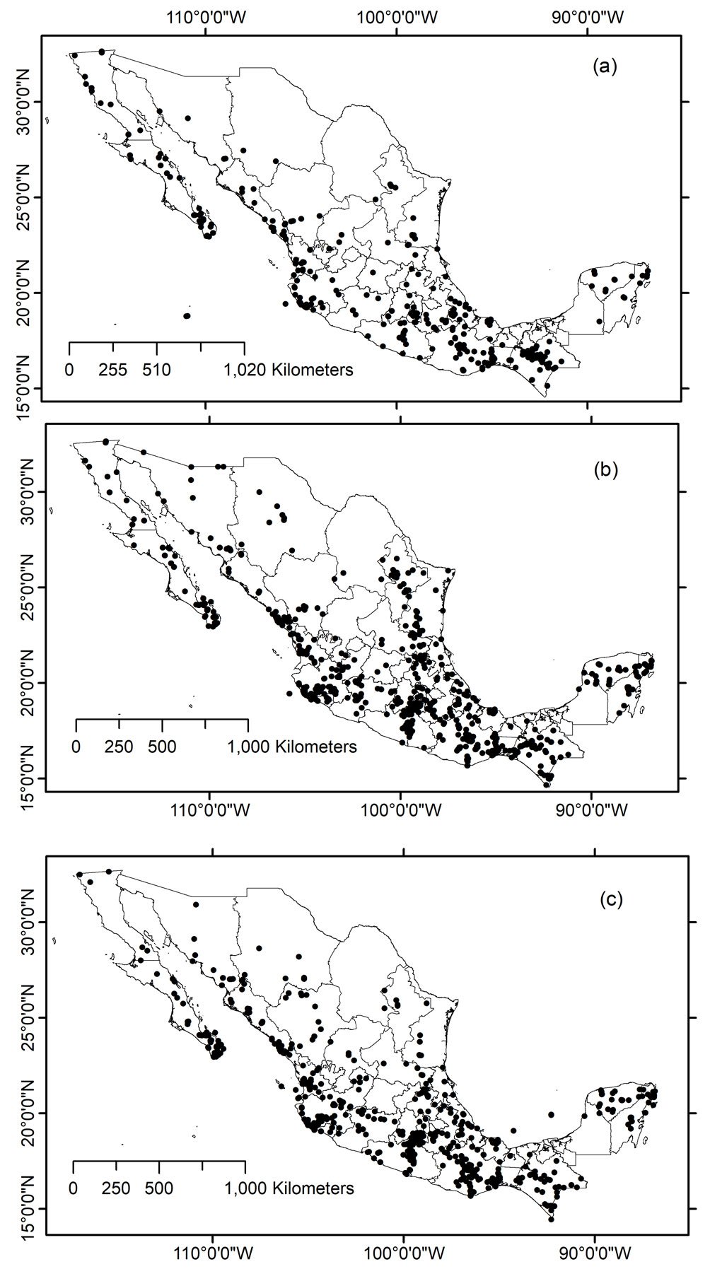
Table 1
Number of Cerambycidae species by state in Mexico.
| State | Species |
| Baja California | 38 |
| Baja California Sur | 62 |
| Campeche | 8 |
| Chiapas | 92 |
| Chihuahua | 8 |
| Coahuila | 4 |
| Colima | 22 |
| Mexico City | 3 |
| Durango | 15 |
| Guanajuato | 2 |
| Guerrero | 67 |
| Hidalgo | 14 |
| Jalisco | 96 |
| Estado de México | 25 |
| Michoacan | 27 |
| Morelos | 45 |
| Nayarit | 49 |
| Nuevo Leon | 17 |
| Oaxaca | 104 |
| Puebla | 36 |
| Queretaro | 3 |
| Quintana Roo | 30 |
| San Luis Potosi | 24 |
| Sinaloa | 47 |
| Sonora | 16 |
| Tabasco | 3 |
| Tamaulipas | 22 |
| Tlaxcala | 1 |
| Veracruz | 66 |
| Yucatan | 33 |
| Zacatecas | 7 |
According to the maxent modelling, some variables showed almost the total contribution percentage in model prediction: For instance, the precipitation of driest month (wc_bio14) had 94% contribution in predicting Phaea acromela and 87% contribution in predicting Eburia brevispinis potential distributions. Similarly, precipitation seasonality (wc_bio15) contributed 79% and 76% for modeling Neocompsa puncticollis asperula and Psyrassa cylindricollis potential distributions, respectively. Other high contribution percentages included: precipitation of wettest month (wc_bio13) had 73% contribution predicting Lagocheirus binumeratus; wc_bio15 had 71% contribution predicting Neocompsa alacris; temperature annual range (wc_bio7) had 71% contribution predicting Lagocheirus araneiformis ypsilon; isothermality (wc_bio3) had 70% contribution predicting Tetraopes umbonatus; wc_bio14 had 61% contribution predicting Lagocheirus procerus; and elevation had 60% contribution predicting Tetraopes femoratus.

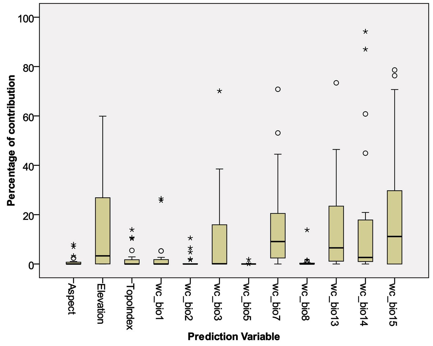
Table 2
Selected prediction variables.
| Bioclimatic variables | |
| wc_bio1 = Annual Mean Temperature | |
| wc_bio2 = Mean Diurnal Range (Mean of monthly [max temp – min temp]) | |
| wc_bio3 = Isothermality (BIO2/BIO7) (×100) | |
| wc_bio5 = Max Temperature of Warmest Month | |
| wc_bio7 = Temperature Annual Range (BIO5-BIO6) | |
| wc_bio8 = Mean Temperature of Wettest Quarter | |
| wc_bio13 = Precipitation of Wettest Month | |
| wc_bio14 = Precipitation of Driest Month | |
| wc_bio15 = Precipitation Seasonality (Coefficient of Variation) | |
| Topographic variables | |
| Elevation | |
| Aspect | |
| Topographic Index |
Considering prediction variables with high contribution percentages for multiple species models, Figure 3 and Table 3 show the most important variables: wc_bio15 (mean = 19%), wc_bio14 (mean = 17%), wc_bio7 (mean = 16%), wc_bio13 (mean = 15%), elevation (mean = 14%), and wc_bio3 (mean = 10%). On the other hand, those prediction variables that had low contribution percentages for fewer species included: Max temperature of warmest month (wc_bio5, mean = 0.09%), mean temperature of wettest quarter (wc_bio8, mean = 0.80%), aspect (mean = 1.06%), mean diurnal range (wc_bio2, mean = 1.07%), topoindex (mean = 2.3%), annual mean temperature (wc_bio1, mean=2.9).
The 4 prediction algorithms, Maximum Entropy (Maxent), Support Vector Machine (SVM), Generalized Linear Model (GLM), and Artificial Neural Networks (ANN) were applied to each of the 24 species that have ≥ 20 records. The models obtained consisted of probability approximations generated by both Modeco and Maxent (ClogLog). The different models for each species were combined by calculating the median value. Then, model accuracy was obtained by calculating the partial ROC test with 500 simulations. These results are shown in Table 4.
In general, the modeled species exhibited high mean AUC ratios and high mean partial AUC values, indicating good model performance, as values of 2.0 and 1.0, respectively, represent a perfect model fit. Mean AUC ratios varied between 1.51 and 1.97, and partial AUC values varied between 0.75 and 0.98. Species with very high mean AUC ratios (> 1.9) included Lagocheirus binumeratus, Psyrassa cylindricollis, Psyrassa sthenias, Neocompsa alacris, Eburia nigrovittata, Euderces batesi. On the other hand, the species with the lowest mean AUC ratios (> 1.5 and < 1.7) were Susuacanga ulkei, Dylobolus rotundicollis, and Tetraopes discoideus.
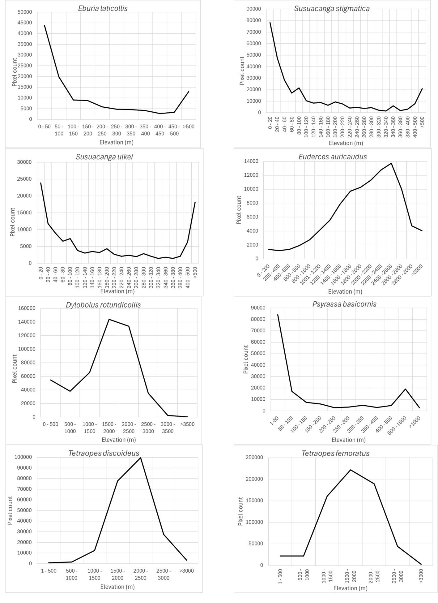
Based on the most important prediction variables identified by the Maxent algorithm, the response variables corresponding to each species model are shown in figures 4-9. For the elevation variable, there were species that preferred elevations between 0 and 50 m: Eburia laticollis, Susuacanga stigmatica, Psyrassa basicornis, and Susuacanga ulkei, which also showed significant predicted areas with elevations above 500 m. On the other hand, there were species selecting distribution areas at much higher elevations: Dylobolus rotundicollis and Tetraopes femoratus at 1,500-2,000 m, Tetraopes discoideus at 2,000-2,500 m, and Euderces auricaudus at 2,400-2,600 m (Fig. 4).
Isothermality (wc_bio3), which is an indicator of daily temperature variation with respect to annual temperature variation, had preferred values < 100 for species models built with this variable as important (35-70%): Highest preferred isothermality values were similar for different species models: Phaea tenuata (65), Euderces batesi (69), Tetraopes umbonatus (70), and Psyrassa sthenias (71) (Fig. 5).
According to Maxent, temperature annual ranges (wc_bio7) were also an important prediction variable for species with different preferring values: 3 species models (Susuacanga stigmatica, Lagocheirus araneiformis, and Psyrassa basicornis) showed temperature annual ranges preferred at 170-180 mm, while Psyrassa sthenias preferred the 18-19ᵒC range. Other species models showed preference for higher temperature annual ranges (Fig. 6): Euderces auricaudus (21-22 ᵒC), Sphaenothecus trilineatus (23-24 ᵒC) and Dylobolus rotundicollis (24-25 ᵒC).
Precipitation of the wettest month (wc_bio13) was another important prediction variable whose highest preferred values varied according to different species: Lagocheirus araneiformis, Dylobolus rotundicollis, Sphaenothecus trilineatus, and Tetraopes discoideus at 150-200 mm; Lagocheirus obsoletus, Mecas obereoides, Phaea tenuata at 200-250 mm; and Lagocheirus binumeratus at 300-350 mm (Fig. 7).
Table 3
Percentage of contribution of each variable in the elaboration of distribution models by the Maxtent algorithm.
| Species | aspect | elevation | topoindex | wc_bio1 | wc_bio2 | wc_bio3 | wc_bio5 | wc_bio7 | wc_bio8 | wc_bio13 | wc_bio14 | wc_bio15 |
| Eburia brevispinis | 0.5 | 0 | 0 | 0 | 4.8 | 0 | 0 | 7.8 | 0 | 0 | 87 | 0 |
| E. laticollis | 0 | 27.4 | 0 | 25.7 | 0 | 0 | 0 | 1.9 | 0 | 0.3 | 11.3 | 33.4 |
| E. nigrovittata | 0 | 0 | 0 | 26.5 | 0 | 0 | 0 | 10.4 | 0 | 2 | 13.5 | 47.6 |
| Susuacanga stigmatica | 0 | 50.2 | 0 | 2.7 | 0 | 0 | 0 | 35.9 | 1.5 | 9.8 | 0 | 0 |
| S. ulkei | 0.1 | 25.8 | 0 | 0 | 0.1 | 2.2 | 0 | 0 | 13.8 | 0 | 44.9 | 13.2 |
| Euderces auricaudus | 0 | 30.7 | 0 | 0 | 0 | 15.3 | 0 | 53.1 | 0.5 | 0 | 0.4 | 0 |
| E. batesi | 0.5 | 24.2 | 0 | 0 | 0 | 35.1 | 1.8 | 19.8 | 0.3 | 15.4 | 3 | 0 |
| Lagocheirus araneiformis ypsilon | 0.3 | 0.1 | 5.5 | 0 | 1.7 | 0 | 0.1 | 70.8 | 0 | 21.1 | 0 | 0.4 |
| L. binumeratus | 7.9 | 0.7 | 0 | 0 | 0 | 0.3 | 0.1 | 17.5 | 0 | 73.4 | 0 | 0 |
| L. obsoletus | 0 | 1.2 | 2.9 | 1 | 0 | 6.1 | 0 | 15.3 | 0 | 46.4 | 16.2 | 10.9 |
| L. procerus | 0 | 4.7 | 0 | 1.4 | 6.5 | 0 | 0 | 1.8 | 0.4 | 13.1 | 60.8 | 11.4 |
| Mecas obereoides | 0 | 0 | 0 | 2.2 | 0 | 0 | 0 | 15.3 | 0 | 37.3 | 1.6 | 43.5 |
| Dylobolus rotundicollis | 0 | 27.1 | 10.3 | 0 | 0 | 0 | 0 | 20.3 | 1.1 | 22.6 | 18.5 | 0 |
| Neocompsa alacris | 0 | 1.9 | 10.7 | 5.3 | 0 | 0 | 0 | 5.6 | 0 | 3.6 | 2.1 | 70.7 |
| N. puncticollis asperula | 7 | 0 | 0 | 0 | 2 | 0 | 0 | 4.7 | 0 | 3.3 | 4.4 | 78.6 |
| Phaea acromela | 3.3 | 0 | 0 | 0 | 0 | 0.2 | 0 | 0 | 0 | 2.4 | 94.2 | 0 |
| P. tenuata | 2.4 | 6.3 | 0.5 | 0 | 0 | 38.5 | 0 | 3.4 | 0 | 43.4 | 2 | 3.5 |
| Psyrassa basicornis | 0 | 26.6 | 0 | 5.3 | 0.1 | 16.5 | 0 | 44.5 | 1.6 | 5.3 | 0.1 | 0 |
| P. cylindricollis | 1 | 9 | 0.6 | 0 | 0 | 0 | 0.1 | 3 | 0 | 7.8 | 2.1 | 76.3 |
| P. sthenias | 2.4 | 0.6 | 0 | 0 | 0 | 35.5 | 0 | 20.7 | 0 | 4.5 | 17.2 | 19.1 |
| Sphaenothecus trilineatus | 0 | 0 | 0.4 | 0.2 | 0 | 14.4 | 0 | 27 | 0 | 25.1 | 20.9 | 12 |
| Tetraopes discoideus | 0 | 41.2 | 10.5 | 0 | 0 | 16.5 | 0 | 1.2 | 0 | 24.3 | 2.3 | 4.1 |
| T. femoratus | 0 | 59.9 | 13.9 | 0 | 10.5 | 0 | 0 | 0 | 0 | 0 | 2.3 | 13.4 |
| T. umbonatus | 0 | 0.4 | 0 | 0 | 0 | 70.1 | 0 | 3.5 | 0 | 0 | 0 | 26 |
| Mean | 1.06 | 14.08 | 2.30 | 2.93 | 1.07 | 10.45 | 0.09 | 15.98 | 0.80 | 15.05 | 16.87 | 19.34 |
| Median | 0.00 | 3.30 | 0.00 | 0.00 | 0.00 | 0.10 | 0.00 | 9.10 | 0.00 | 6.55 | 2.65 | 11.15 |
| Standard deviation | 2.17 | 18.15 | 4.35 | 7.31 | 2.60 | 17.81 | 0.37 | 18.62 | 2.81 | 18.89 | 27.21 | 25.63 |
Table 4
Partial ROC results for modeled species.
| Species | Mean AUC ratio | Mean partial AUC |
| Eburia brevispinis | 1.884237 | 0.9420767 |
| E. laticollis | 1.857125 | 0.9285514 |
| E. nigrovittata | 1.939383 | 0.9696851 |
| Susuacanga stigmatica | 1.738087 | 0.869013 |
| S. ulkei | 1.512725 | 0.7563525 |
| Euderces auricaudus | 1.822893 | 0.9114264 |
| E. batesi | 1.972096 | 0.9860455 |
| Lagocheirus araneiformis ypsilon | 1.789459 | 0.8944192 |
| L. binumeratus | 1.909858 | 0.9549165 |
| L. obsoletus | 1.772241 | 0.886116 |
| L. procerus | 1.749532 | 0.8747619 |
| Mecas obereoides | 1.767577 | 0.8837588 |
| Dylobolus rotundicollis | 1.664294 | 0.8320284 |
| Neocompsa alacris | 1.938096 | 0.9690422 |
| N. puncticollis asperula | 1.883306 | 0.9416244 |
| Phaea acromela | 1.866931 | 0.9334454 |
| P. tenuata | 1.776351 | 0.888124 |
| Psyrassa basicornis | 1.871859 | 0.9359075 |
| P. cylindricollis | 1.919474 | 0.9597301 |
| P. sthenias | 1.921234 | 0.9606008 |
| Sphaenothecus trilineatus | 1.876181 | 0.9380483 |
| Tetraopes discoideus | 1.680489 | 0.8401879 |
| T. femoratus | 1.815506 | 0.907635 |
| T. umbonatus | 1.707098 | 0.8535488 |
The precipitation of the driest month (wc_bio14) was also an important prediction variable for which its response variable took the highest preferred values between 0 and 25-50 mm: Susuacanga ulkei and Lagocheirus procerus showed the highest preferred values of 0 mm, Dylobolus rotundicollis and Sphaenothecus trilineatus at 3 mm, and Eburia brevispinis and Phaea acromela at 25-50 mm (Fig. 8).
Finally, the precipitation seasonality (wc_bio15), which is the coefficient of variation of precipitation, was an important prediction variable whose preferred highest values (110) seem similar for this group of species (Fig. 9): Eburia laticollis, Eburia nigrovittata, Mecas obereoides, Neocompsa alacris, Neocompsa puncticollis asperula, and Psyrassa cylindricollis.
A composite map was generated by adding each of 24 binary species distribution models (Fig. 10). In general, species that highly concurred (16-21 spp.) in only 2 very confined areas, located in southern Sinaloa and southern Oaxaca. On the other hand, large areas with no species concurring were in northern Mexico (Fig. 10). This richness map was cross-tabulated with the ecoregion map to show the biomes associated with the different concurring intervals (Fig. 11). Each richness interval was tabulated for different ecoregions, showing that the highest range (16-21 spp.) corresponded to the tropical dry forest in 75% and the tropical humid forest in 24%. The second highest interval (11-15 spp.) corresponded again to the tropical dry forest (69%), but this time, the temperate mountains were in the second place with 17%, and the tropical humid forest with 14%. On the other hand, the areas with no species concurrence corresponded to the North American Desert (45%), followed by the Great Plains (21%), temperate mountains (12%), and semi-desert (11%). The tropical dry forest occupied 8% of such areas with no species concurrence, while the tropical humid forest occupied only 0.2%.
Discussion
Considering the original number of records included in the databases (> 10,000) along with the localities, both georeferenced and without geographic coordinates, and the number of species, there was the expectation to obtain a database with a significant number of species and records. However, there existed a very limited number of species (24) with enough records (≥ 20) to be used in modeling species potential distribution. In fact, the species with ≥ 5 and < 20 records were also limited (124), and the bulk of species (266) had < 5 records (Supplementary material: A2). It is evident that extensive taxonomic fieldwork is necessary to document the species diversity of Cerambycidae in Mexico. In this regard, and apparently supporting this pattern of records, 7.4% of the species recorded in Mexico have no locality records in the country, 45.5% have been recorded in only one state, and 16% in 2 states. This means that nearly 69% of the species have either a restricted distribution or are poorly studied in terms of their distribution (F. A. Noguera, unpublished data).
By mapping the geographic location of Cerambycidae species records in Mexico, it is noteworthy that the sampling intensity does not necessarily reflect the intensity of sampling, as the information included primarily corresponds to taxonomically studied groups rather than studies aimed at documenting the diversity of the different regions of the country, and sampling gaps are revealed by state and ecoregion across the country. In fact, the map somewhat confirms the current knowledge about the diversity of this group in the various states of the republic (Martínez-Hernández et al., 2024; Noguera, 2014; Noguera unpublished data). For example, in fact, 565 species have been recorded in Oaxaca, 485 in Veracruz, 435 in Chiapas, 397 in Jalisco, 283 in Guerrero, and 216 in Morelos —states with the highest number of records included in the study. In contrast, states such as Tlaxcala (10 species), Campeche (11), Aguascalientes (12), Tabasco (21), Zacatecas (26), Guanajuato (33), Coahuila (35), Mexico City (36), Nuevo León (69), and Chihuahua (73) recorded the fewest species in this study.
In the ≥ 20 records per species group, the most sampled biome was the tropical dry forest (348 records and 23 species), while the temperate forests included 21 species with 140 records.
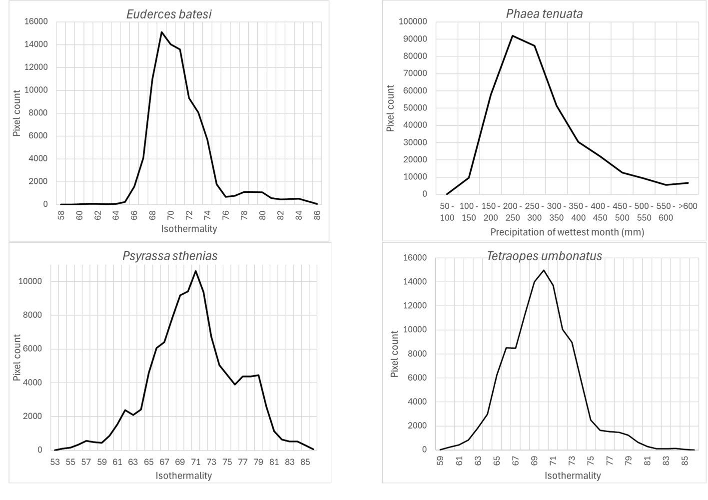
The 24 species distribution models primarily represent examples of this family’s species that are better sampled in the country. Different from relying on a single prediction algorithm, this study presents consensus models, generated from combining probability versions of 4 algorithms: Maxent, Artificial Neural Networks, Generalized Linear Model, and Support Vector Machine. The median was the statistic chosen for combining the 4 algorithms because of its characteristic of being a location parameter in contrast with the mean, which combines in-depth partial values, and is affected by outliers. Although the variations among models for the same species were evident, all 24 species distribution models showed good performance, as indicated by the AUC ratios and partial AUC values.
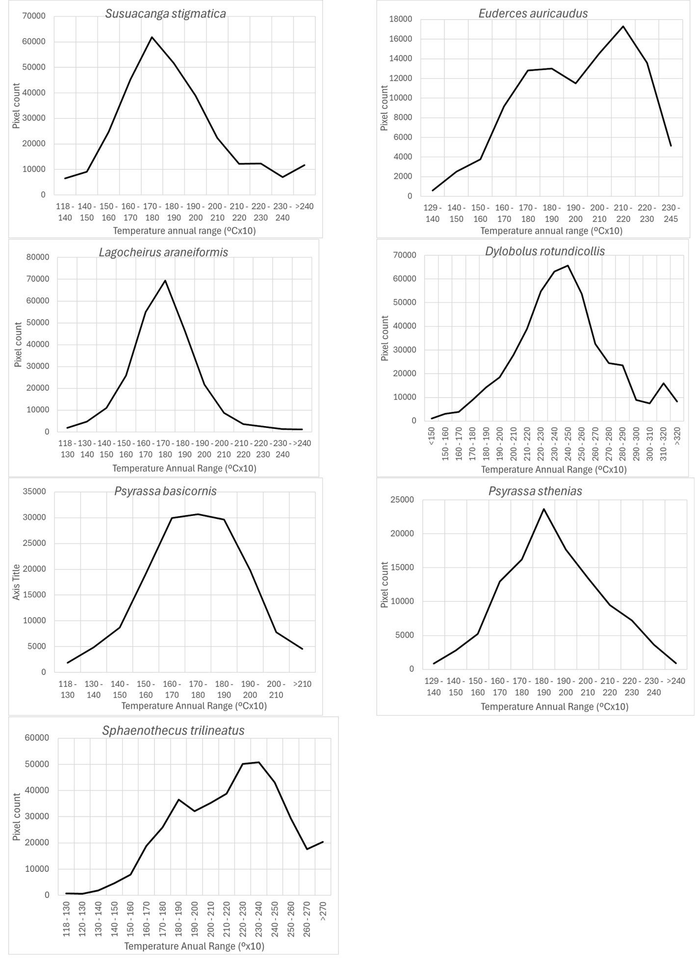
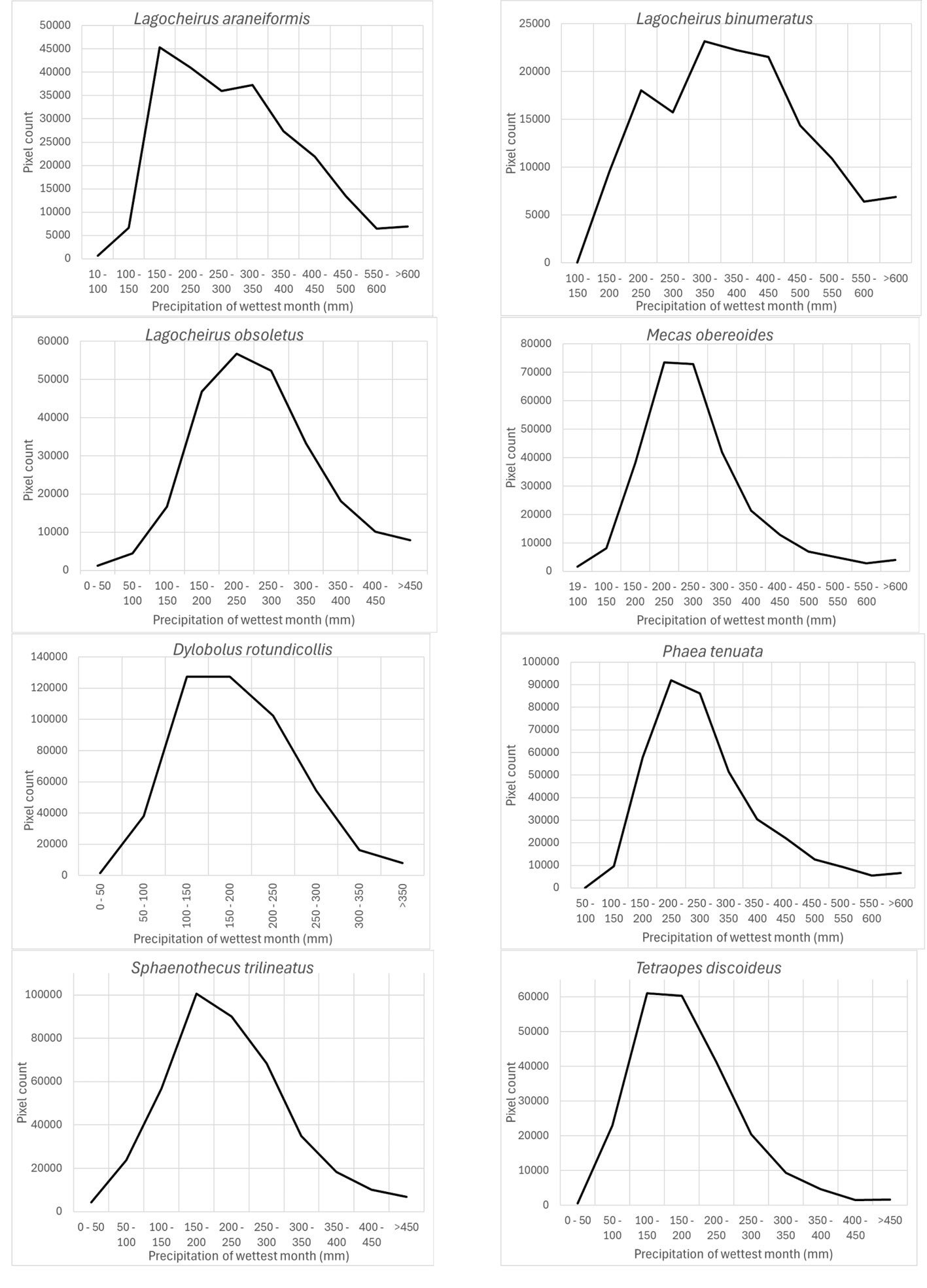
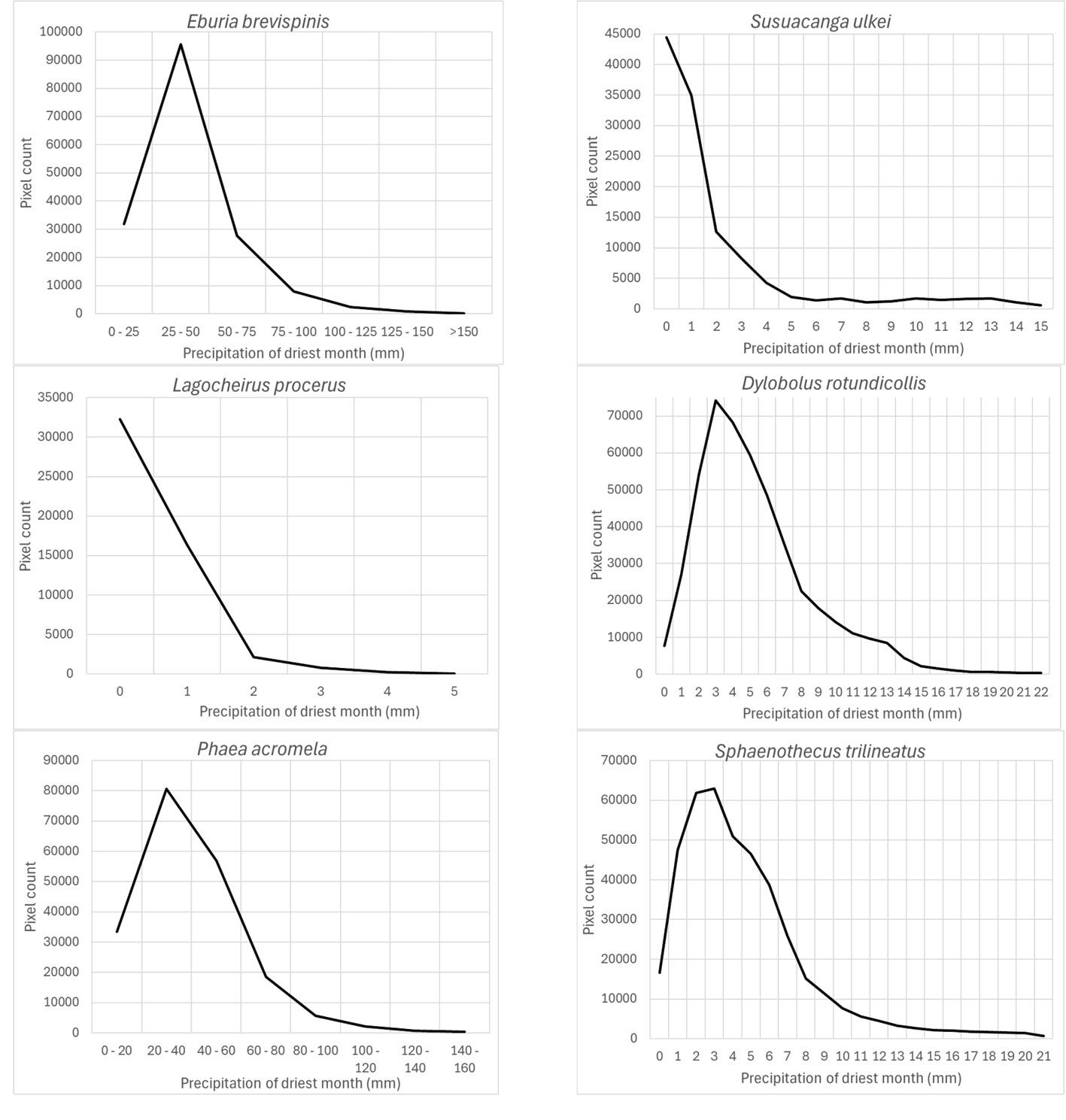
According to Maxent, prediction variables differed in importance for predicting species potential distribution models. The variables that had higher mean importance among species included precipitation seasonality (wc_bio15), precipitation of driest month (wc_bio14), temperature annual range (wc_bio7), precipitation of wettest month (wc_bio13), elevation, and isothermality (wc_bio3). As in this case, other studies on Cerambycidae, where the potential distribution of some species in this group was modeled, also showed that the predictive bioclimatic variables were diverse and contributed to the models to varying degrees. For example, for Psacothea hilaris, the predictive variables were precipitation of the warmest quarter (wc_bio18) and isothermality (wc_bio3) (Ruzzier et al., 2024); for Rosalia alpina, they were elevation and mean temperature of the driest quarter (wc_bio9) (Bosso et al., 2018); for Morimus asper, they were the maximum temperature during the warmest month (wc_bio5) and altitude (Kostova et al., 2023); for Batocera lineolata, they were maximum temperature in January, precipitation in July, and temperature seasonality (wc_bio4) (Li et al., 2020); for Xylotrechus arvicola, they were precipitation in October, mean maximum temperature in January, mean minimum temperature in July, mean maximum temperature, and mean minimum temperature in August (Felicísimo et al., 2021); for Monochamus carolinensis, they were precipitation of the warmest quarter (wc_bio18), precipitation seasonality (wc_bio15), precipitation of the coldest quarter (wc_bio19), mean diurnal range (wc_bio2), and minimum temperature of the coldest month (wc_bio5) (Zhao et al., 2023). This recorded variety in predictive environmental variables corresponds to the region where each of these studies was conducted. For P. hilaris, the main areas were Italy and the Mediterranean region; for R. alpina, it was Europe; for M. asper, it was Bulgaria; for B. lineolata, it was China; for X. arvicola, it was Spain; and for M. carolinensis, it was on a global scale.
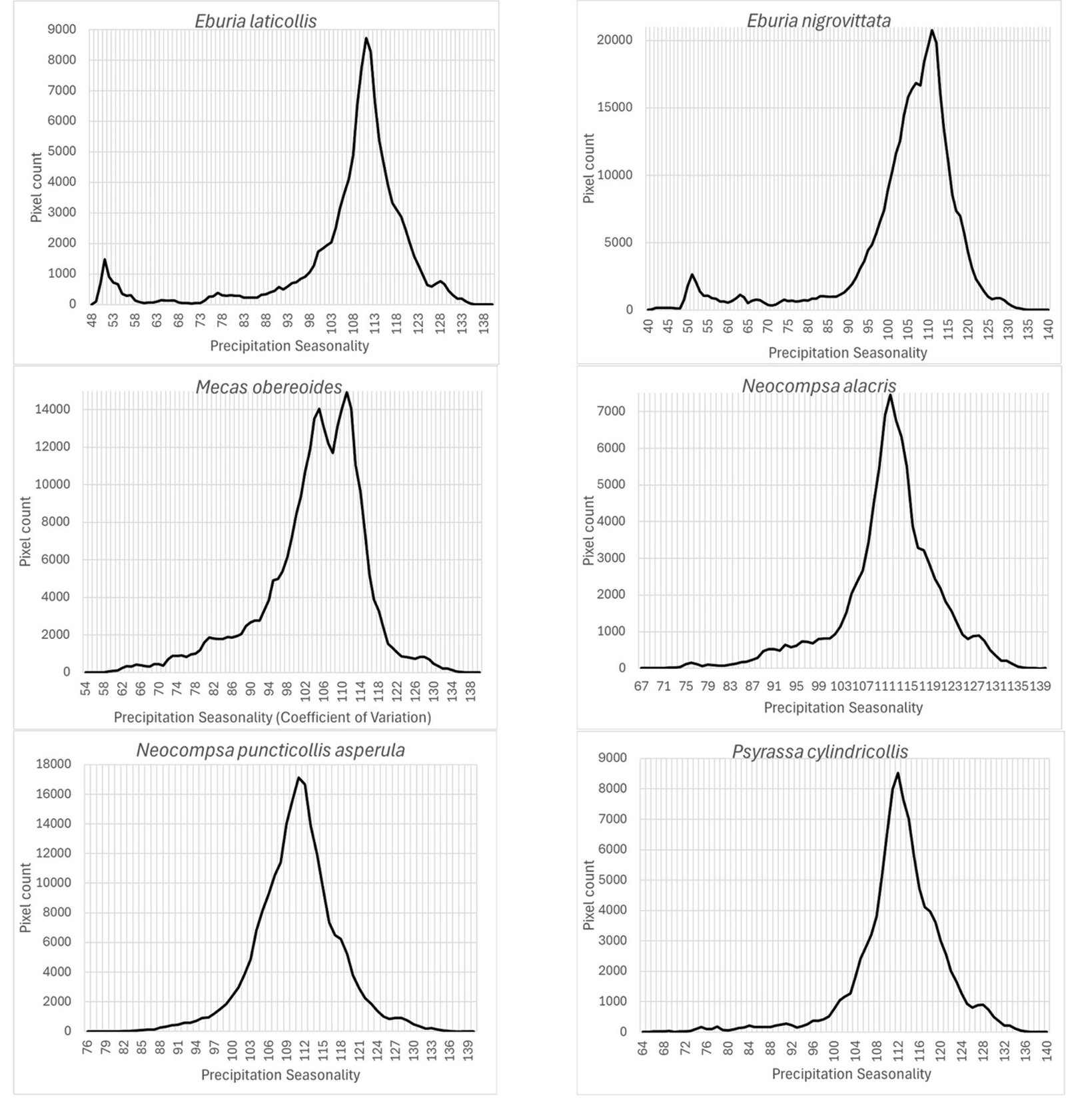
The response variables obtained by cross-tabulating the species presence models with the environmental (prediction) variables identify the most favorable habitat conditions, according to the predicted distribution models. Even though the most frequent values of the environmental variables indicate which areas dominated the species distribution, the range of such values provides an estimate of the span of environmental values where species can occur.
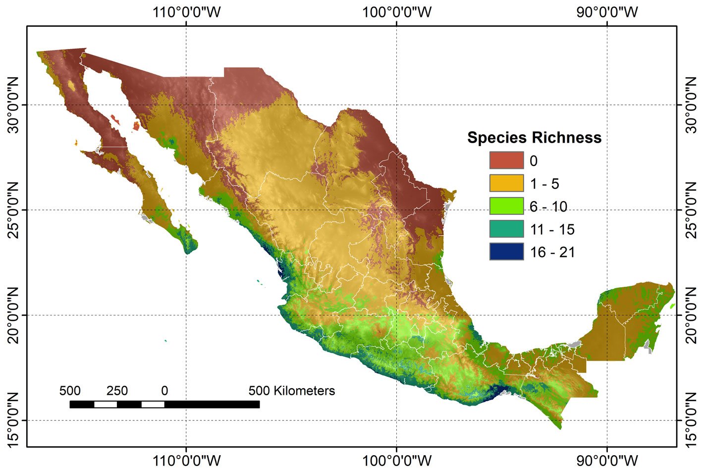
The 24 modeled species showed spatial correspondence, where the highest interval (16-21 species) is confined to restricted areas with tropical and humid tropical forests in the country. Larger species spatial correspondence areas corresponded to the lowest intervals (1-5 and 6-10 species), which were distributed in the tropical dry forest and temperate forests. It is worth mentioning that biomes such as the North American deserts and the Great Plains showed the highest proportion of areas with the absence of species.
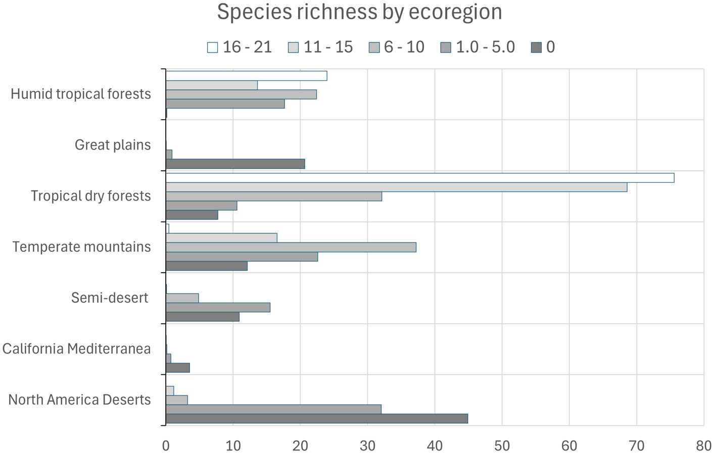
References
Anderson, R. P., & Martı́nez-Meyer, E. (2004). Modeling species’ geographic distributions for preliminary conservation assessments: an implementation with the spiny pocket mice (Heteromys) of Ecuador. Biological Conservation, 116, 167–179. https://doi-org.pbidi.unam.mx:2443/10.1016/S0006-3207(03)00187-3
Araújo, M. B., & New, M. (2007). Ensemble forecasting of species distributions. Trends in Ecology & Evolution, 22, 42–47. https://doi.org/10.1016/j.tree.2006.09.010
Austin, M. P. (2002). Spatial prediction of species distribution: an interface between ecological theory and statistical modelling. Ecological Modelling, 157, 101–118. https://doi.org/10.1016/S0304-3800(02)00205-3
Ballesteros-Mejia, L., Kitching, I. J., Jetz, W., Nagel, P., & Beck, J. (2013). Mapping the biodiversity of tropical insects: species richness and inventory completeness of African sphingid moths. Global Ecology and Biogeography, 22, 586–595. https://doi.org/10.1111/geb.12039
Ballesteros-Mejia, L., Kitching, I. J., Jetz, W., & Beck, J. (2017). Putting insects on the map: near-global variation in sphingid moth richness along spatial and environmental gradients. Ecography, 40, 698–708. https://doi.org/10.1111/ecog.02438
Barredo, J. I., Strona, G., De Rigo, D., Caudullo, G., Stancanelli, G., & San-Miguel-Ayanz, J. (2015). Assessing the potential distribution of insect pests: case studies on large pine weevil (Hylobius abietis L) and horse-chestnut leaf miner (Cameraria ohridella) under present and future climate conditions in European forests. EPPO Bulletin, 45, 273–281. https://doi.org/10.1111/epp.12208
Bezark, L. G., & Monné, M. A. (2013). Checklist of the Oxypeltidae, Vesperidae, Disteniidae and Cerambycidae, (Coleoptera) of the Western Hemisphere. Retrieved from: http://bezbycids.com/byciddb/checklists/WestHemiCerambycidae2024.pdf
Bosso, L., Smeraldo, S., Rapuzzi, P., Sama, G., & Garonna, A. P. (2018). Nature protection areas of Europe are insufficient to preserve the threatened beetle Rosalia alpina (Coleoptera: Cerambycidae): evidence from species distribution models and conservation gap analysis. Ecological Entomology, 43, 192–203. https://doi.org/10.1111/een.12485
Buse, J., Schröder, B., & Assmann, T. (2007). Modelling habitat and spatial distribution of an endangered longhorn beetle-A case study for saproxylic insect conservation. Biological Conservation, 137, 372–381. https://doi.org/10.1016/j.biocon.2007.02.025
Catalano, G. A., D’Urso, P. R., Maci, F., & Arcidiacono, C. (2023). Influence of parameters in SDM application on citrus presence in mediterranean area. Sustainability, 15, 7656. https://doi.org/10.3390/su15097656
Crawford, P. H. C., & Hoagland, B. W. (2010). Using species distribution models to guide conservation at the state level: the endangered American burying beetle (Nicrophorus americanus) in Oklahoma. Journal of Insect Conservation, 14, 511–521. https://doi.org/10.1007/s10841-010-9280-8
Colwell, R. K. (1996). Biota: the biodiversity database manager. Sinauer Associates, Sunderland, Massachusetts. Systematic Biology, 46, 574–575.
D’Amen, M., Pradervand, J. N., & Guisan, A. (2015). Predicting richness and composition in mountain insect communities at high resolution: a new test of the SESAM framework. Global Ecology and Biogeography, 24, 1443–1453. https://doi.org/10.1111/geb.12357
Drake, J. M., Randin, C., & Guisan, A. (2006). Modelling ecological niches with support vector machines. Journal of Applied Ecology, 43, 424–432. https://doi.org/10.1111/
j.1365-2664.2006.01141.x
Elith, J., Graham, C. H., Anderson, R. P., Dudík, M., Ferrier, S., Guisan, A. et al. (2006). Novel methods improve prediction of species’ distributions from occurrence data. Ecography,
29, 129–151. https://doi.org/10.1111/j.2006.0906-7590.04596.x
Eickermann, M., Junk, J., & Rapisarda, C. (2023). Climate change and insects. Insects, 14, 678. https://doi.org/10.3390/insects14080678
Elith, J., & Graham, C. H. (2009). Do they? How do they? Why do they differ? On finding reasons for differing performances of species distribution models. Ecography, 32, 66–77. https://doi.org/10.1111/j.1600-0587.2008.05505.x
Felicísimo, A. M., Armendáriz, I., & Alberdi, V. (2021). Modelling the potential effects of climate change in the distribution of Xylotrechus arvicola in Spain. Horticultural Science (Prague), 48, 38–46. https://doi.org/10.17221/85/2019-HORTSCI
Fick, S. E., & Hijmans, R. J. (2017). WorldClim 2: new 1-km spatial resolution climate surfaces for global land areas. International Journal of Climatology, 37, 4302–4315. https://doi.org/10.1002/joc.5086
Franklin, J. (2010). Mapping species distributions. Spatial inference and prediction. Cambridge UK: Cambridge University Press. https://doi.org/10.1017/CBO9780511810602
Graham, C. H., Ferrier, S., Huettman, F., Moritz, C., & Peterson, A. T. (2004). New developments in museum-based informatics and applications in biodiversity analysis. Trends in Ecology & Evolution, 19, 497–503. https://doi.org/10.1016/j.tree.2004.07.006
Guisan, A., & Zimmermann, N. E. (2000). Predictive habitat distribution models in ecology. Ecological Modelling, 135, 147–186. https://doi.org/10.1016/S0304-3800(00)00354-9
Guisan, A., Edwards, T. C., & Hastie, T. (2002). Generalized linear and generalized additive models in studies of species distributions: setting the scene. Ecological Modelling, 157, 89–100. https://doi.org/10.1016/S0304-3800(02)00204-1
Guo, Q., Kelly, M., & Graham, C. H. (2005). Support vector machines for predicting distribution of Sudden Oak Death in California. Ecological Modelling, 182, 75–90. https://doi.org/10.1016/j.ecolmodel.2004.07.012
Guo, Q., & Liu, Y. (2010). ModEco: an integrated software package for ecological niche modeling. Ecography, 33, 637–642. https://doi.org/10.1111/j.1600-0587.2010.06416.x
Hassall, C. (2012). Predicting the distributions of under-recorded Odonata using species distribution models. Insect Conservation and Diversity, 5, 192–201. https://doi.org/10.1111/j.1752-4598.2011.00150.x
Hastie, T., Tibshirani, R., & Friedman, J. (2001). The elements of statistical learning: data mining, inference, and prediction.
New York: Springer. https://doi.org/10.1007/978-0-387-21606-5
Hijmans, R. J., Cameron, S. E., Parra, J. L., Jones, P. G., & Jarvis, A. (2005). Very high resolution interpolated climate surfaces for global land areas. International Journal of Climatology: A Journal of the Royal Meteorological Society, 25, 1965–1978. https://doi.org/10.1002/joc.1276
Huntley, B., Green, R. E., Collingham, Y. C., Hill, J. K., Willis, S. G., Bartlein, P. J. et al. (2004). The performance of models relating species geographical distributions to climate is independent of trophic level. Ecology Letters, 7, 417–426. https://doi.org/10.1111/j.1461-0248.2004.00598.x
Jung, J. M., Lee, W. H., & Jung, S. (2016). Insect distribution in response to climate change based on a model: Review of function and use of CLIMEX. Entomological Research, 46, 223–235. https://doi.org/10.1111/1748-5967.12171
Kostova, R., Bekchiev, R., Popgeorgiev, G., & Kornilev, Y. V. (2023). First exhaustive distribution and habitat modelling of Morimus asper (Sulzer, 1776) sensu lato (Coleoptera, Cerambycidae) in Bulgaria. Nature Conservation, 53, 39–59. https://doi.org/10.3897/natureconservation.53.104243
Lek, S., Delacoste, M., Baran, P., Dimopoulos, I., Lauga, J., & Aulagnier, S. (1996). Application of neural networks to modelling nonlinear relationships in ecology. Ecological Modelling,90, 39–52. https://doi.org/10.1016/0304-3800(95)00142-5
Li, A., Wang, J., Wang, R., Yang, H., Yang, W., Yang, C. et al. (2020). MaxEnt modeling to predict current and future distributions of Batocera lineolata (Coleoptera: Cerambycidae) under climate change in China. Écoscience, 27, 23–31. https://doi.org/10.1080/11956860.2019.1673604
Linsley, E. G. (1961). The Cerambycidae of North America. Part I. Introduction. University of California Publications in Entomology, 18, 1–135.
Lobo, J. M. (2016). The use of occurrence data to predict the effects of climate change on insects. Current Opinion in Insect Science, 17, 62–68. https://doi.org/10.1016/j.cois.
2016.07.003
Lobo, J. M., Lumaret, J. P., & Jay-Robert, P. (2002). Modelling the species richness distribution of French dung beetles (Coleoptera, Scarabaeidae) and delimiting the predictive capacity of different groups of explanatory variables. Global Ecology and Biogeography, 11, 265–277. https://doi.org/10.1046/j.1466-822X.2002.00291.x
Ma, G., & Ma, C. S. (2022). Potential distribution of invasive crop pests under climate change: incorporating mitigation responses of insects into prediction models. Current
Opinion in Insect Science, 49, 15–21. https://doi.org/10.1016/j.cois.2021.10.006
Martínez-Hernández, J. G., Rös, M., Pérez-Flores, O., & Toledo-Hernández, V. H. (2024). Checklist of the Cerambycidae (Coleoptera: Chrysomeloidea) of Oaxaca, Mexico. Zootaxa, 5405, 185–208. https://doi.org/10.11646/zootaxa.5405.2.2
Monné, M. A. (2005). Catalogue of the Cerambycidae (Coleoptera) of the Neotropical region. Part I. Subfamily Cerambycinae. Zootaxa, 946, 17–65. https://doi.org/10.11646/zootaxa.946.1.1
Müller, K. R., Mika, S., Tsuda, K., & Schölkopf, K. (2002). An introduction to Kernel-based learning algorithms. In Yu Hen Hu, & Jenq-Neng Hwang (Eds.), Handbook of neural network signal processing. Boca-Raton: CRC Press. https://doi.org/10.1201/9781315220413
Nearns, E. H., Lord, N. P., Lingafelter, S. W., Santos, A., Miller, K. B., & Zaspel, J. M. (2017). LONGICORN ID. Retrieved from: https://cerambycids.com
Noguera, F. A. (2014). Biodiversidad de Cerambycidae (Coleoptera) en México. Revista Mexicana de Biodiversidad, 85 (Supl.), S290–S297. https://doi.org/10.7550/rmb.32966
Norberg, A., Abrego, N., Blanchet F. G., Adler, F. R., Anderson, B. J., Anttila, J. et al. (2019). A comprehensive evaluation of predictive performance of 33 species distribution models at species and community levels. Ecological Monographs, 89, e01370. https://doi.org/10.1002/ecm.1370
Peterson, A. T., Papeş, M., & Soberón, J. (2008). Rethinking receiver operating characteristic analysis applications in ecological niche modeling. Ecological Modelling, 213, 63–72. https://doi.org/10.1016/j.ecolmodel.2007.11.008
Phillips, S. J., Anderson, R. P., & Schapire, R. E. (2006). Maximum entropy modeling of species geographic distributions. Ecological Modelling, 190, 231–259. https://doi.org/10.1016/j.ecolmodel.2005.03.026
Phillips, S. J., Anderson, R. P., Dudík, M., Schapire, R. E., & Blair, M. E. (2017). Opening the black box: an open-source release of Maxent. Ecography, 40, 887–893. https://doi.org/10.1111/ecog.03049
Phillips, S. J., & Dudík, M. (2008). Modeling of species distributions with Maxent: new extensions and a comprehensive evaluation. Ecography, 31, 161–175. https://doi.org/10.1111/j.0906-7590.2008.5203.x
Pouteau, R., Meyer, J. Y., Taputuarai, R., & Stoll, B. (2012). Support vector machines to map rare and endangered
native plants in Pacific islands forests. Ecological Informatics, 9, 37–46. https://doi.org/10.1016/j.ecoinf.2012.03.003
Ruzzier, E., Lupi, D., Tirozzi, P., Dondina, O., Orioli V., Jucker, C. et al. (2024). A two‑step species distribution modeling to disentangle the effect of habitat and bioclimatic covariates on Psacothea hilaris, a potentially invasive species. Bio Invasions, 26, 1861–1881. https://doi.org/10.1007/s10530-024-03283-9
Schölkopf, B., Platt, J. C., Shawe-Taylor, J., Smola, A. J., & Williamson, R. C. (2001). Estimating the support of a high-dimensional distribution. Neural Computation, 13, 1443–1471. https://doi.org/10.1162/089976601750264965
Senay, S. D., & Worner, S. P. (2019). Multi-scenario species distribution modeling. Insects, 10, 65. https://doi.org/10.3390/insects10030065
Silva, D. P., Aguiar, A. G., & Simião-Ferreira, J. (2016). Assessing the distribution and conservation status of a long-horned beetle with species distribution models. Journal of Insect Conservation, 20, 611–620. https://doi.org/10.1007/s10841-016-9892-8
Toledo, V. H., & Corona, A. M. (2006). Patrones de distribución de la familia Cerambycidae (coleóptera). In J. J. Morrone, & J. Llorente Bosques (Eds.), Componentes bióticos principales de la entomofauna mexicana, México (pp. 425–474). México D.F.: Las Prensas de Ciencias, UNAM.
Ulrichs, C., & Hopper, K. R. (2008). Predicting insect distributions from climate and habitat data. BioControl, 53, 881–894. https://doi.org/10.1007/s10526-007-9143-8
Urbani, F., D’alessandro, P., & Biondi, M. (2017). Using Maximum Entropy Modeling (MaxEnt) to predict future trends in the distribution of high altitude endemic insects in response to climate change. Bulletin of Insectology, 70, 189–200.
Valavi, R., Guillera-Arroita, G., Lahoz-Monfort, J. J., & Elith, J. (2022). Predictive performance of presence-only species distribution models: a benchmark study with reproducible code. Ecological Monographs, 92, e01486. https://doi.org/10.1002/ecm.1486
Watts, M. J., & Worner, S. P. (2008). Comparing ensemble and cascaded neural networks that combine biotic and abiotic variables to predict insect species distribution. Ecological Informatics, 3, 354–366. https://doi.org/10.1016/j.ecoinf.2008.08.003
Williams, J. N., Seo, C., Thorne, J., Nelson, J. K., Erwin, S., O’Brien, J. M. et al. (2009). Using species distribution models to predict new occurrences for rare plants. Diversity and Distributions, 15, 565–576. https://doi.org/10.1111/j.1472-4642.2009.00567.x
Zaniewski, A. E., Lehmann, A., & Overton, J. M. (2002). Predicting species spatial distributions using presence-only data: a case study of native New Zealand ferns. Ecological Modelling, 157, 261–280. https://doi.org/10.1016/S0304-3800(02)00199-0
Zhao, J., Zou, X., Yuan, F., Luo, Y., & Shi, J. (2023). Predicting the current and future distribution of Monochamus carolinensis (Coleoptera: Cerambycidae) based on the maximum entropy model. Pest Management Science, 79, 5393–5404. https://doi.org/10.1002/ps.7753

Macroalgae assemblages in different reef zones of a tropical urban beach in Brazil
Ensambles de macroalgas en diferentes zonas arrecifales de una playa urbana tropical en Brasil
Caio Ceza da Silva-Nunes a, c, d, e, *, Edilene Maria dos Santos Pestana b, c, Cibele Conceição dos Santos b, c, Lorena Pedreira Conceição a, c, José Marcos de Castro Nunes a, c
a Universidade Estadual de Feira de Santana, Departamento de Ciências Biológicas, Programa de Pós-Graduação em Botânica, Av. Transnordestina s/n, Novo Horizonte, CEP 44036-900, Feira de Santana, Bahia, Brazil
b Universidade Federal da Bahia, Instituto de Biologia, Programa de Pós-Graduação em Biodiversidade e Evolução, Rua Barão de Jeremoabo, 668 – Campus de Ondina, CEP: 40170-115, Salvador, Bahia, Brazil
c Universidade Federal da Bahia, Instituto de Biologia, Laboratório de Algas marinhas, Rua Barão de Jeremoabo, 668 – Campus de Ondina, CEP: 40170-115, Salvador, Bahia, Brazil
d Universidade Estadual do Sudoeste da Bahia, Departamento de Ciências Exatas e Naturais, Programa de Pós-Graduação em Ciências Ambientais, Campus Universitário “Juvino Oliveira”, BR 415, Km 04 CEP: 45.700-000 Itapetinga, Bahia, Brazil
e Colégio Estadual de Tempo Integral Antônio Batista, Rua Presidente Vargas, 83 CEP: 46380-076 Candiba, Bahia, Brazil
*Corresponding author: caiobio08@gmail.com (C.C. da Silva-Nunes)
Received: 26 February 2025; accepted: 01 August 2025
Abstract
Marine macroalgae are commonly used as bioindicators because they are sensitive to environmental changes. This study aims to verify the composition of macroalgae in the intertidal region in 3 reef zones on Itapuã beach, located in Salvador-Bahia, Brazil and which presents high tourist activity. The samples were obtained in July 2017, in the intertidal zone, in 3 reef regions: Protected Region (PR), Tide Pool Region (TP) and Frontal Region (FR). In each zone, 3 transects (20 m each) were placed, in which 5 squares measuring 20 x 20 cm were arranged at random points. Additionally, individuals were collected around each transect for qualitative analysis. Dry biomass was measured, and statistical tests were carried out to obtain diversity, equitability and similarity data. Fifty-two taxa were identified, 27 Rhodophyta, 16 Chlorophyta and 9 Phaeophyceae. TP had the highest species richness (34) and diversity; however, no significant differences were found in macroalgal biomass between the 3 reef zones analyzed. This study contributes to the understanding of the composition and structure of phytobenthic communities in intertidal regions of the Bahian coast.
Keywords: Bahia; Bioindicator; Brazil; Phytobenthos
Resumen
Las macroalgas marinas se utilizan comúnmente como bioindicadores porque son sensibles a los cambios ambientales. Este estudio tiene como objetivo verificar la composición de macroalgas en la zona intermareal en 3 regiones arrecifales de la playa de Itapuã, ubicada en Salvador-Bahía, Brasil y que tiene alta actividad turística. Las muestras fueron obtenidas en julio de 2017, en la zona intermareal, en 3 regiones arrecifales: región posterior (PR), pozas de marea (TP) y región frontal (FR). En cada región, se colocaron 3 transectos (de 20 m cada uno), donde se distribuyeron aleatoriamente 5 cuadrantes de 20 x 20cm. Además, se recolectaron individuos alrededor de cada transecto para análisis cualitativo. Se midió la biomasa seca y se realizaron pruebas estadísticas para obtener datos de diversidad, equitabilidad y similitud. Se identificaron 52 taxones: 27 Rhodophyta, 16 Chlorophyta y 9 Phaeophyceae. La TP presentó la mayor riqueza de especies (34) y diversidad; sin embargo, no se encontraron diferencias significativas en la biomasa de macroalgas entre las 3 regiones arrecifales. Este estudio contribuye a la comprensión de la composición y estructura de las comunidades fitobentónicas en zonas intermareales del litoral bahiano.
Palabras clave: Bahia; Bioindicador; Brasil; Fitobentos
Introduction
The State of Bahia has the longest coastline in Brazil, 1,103 km showing a great diversity of environments: sandy beaches, coral reefs, sandstone formations, rocky shores and mangroves (Nunes & Paula, 2004a). Furthermore, it is a region that presents a great diversity of substrates and geographical features, which is reflected in the diversity of marine flora (Nunes, 2005b). Nunes and Paula (2002) divided reef formations into 3 zones: Frontal Region (FR), Protected Region (PR) and Tide Pool Region (TP). The FR is a very hydrodynamic region, where direct collision of waves occurs. The PR is the region before the lagoon and after the reef top, it may have pools and is a region protected from direct wave collision. The TP is deep and may suffer greater wave action, forming pools on the reef top, or may suffer less or no wave action, forming pools on the reef plateau.
In recent decades, coastal areas have been undergoing an intense process of urban development, which has caused significant environmental pressures and impacts, especially in benthic communities in reef formations (Costa et al., 2012; Nascimento, 2013). In Salvador, these impacts come from urban expansion, real estate speculation, tourism, human activities, such as fishing and trampling, causing the degradation of the flora and a reduction in the richness and diversity of species, especially in the composition and structure of algal communities.
Marine macroalgal communities have a great ecological role, being, together with microalgae, at the base of the food chain as primary producers, being a source of food for a large part of the marine fauna. The presence of macroalgae along the coast is responsible for softening the impact of waves on the sea coast, and also plays the role of habitat for other organisms, such as animals or as a substrate for algae (Nunes, 2010; Pedrine, 2013).
When these organisms are exposed to some human interference, they are sensitive to changes in their habitat, such as the increase in the concentration of organic matter in the water, which leads to an increase in the biomass of some algal groups, or even the depletion of some nutrient that causes the disappearance of a certain species, working as bioindicators of environmental quality. In addition, the degradation of this community’s structure favors the emergence and persistence of more resistant and opportunistic species, as well as the exclusion of more fragile species (Nascimento, 2013; Nunes, 2010).
Functional groups of algae are based on similarities in their morphological and anatomical characteristics, in addition to their ecological characteristics. Steneck and Dethier (1994) grouped algae into 7 categories, these being microalgae, filamentous, foliaceous, cylindrical-corticate, coriaceous, articulated calcareous and encrusting. In the model proposed by Steneck and Dethier (1994), it is highlighted that environments of high productivity and low disturbance present high biomass and diversity of morphofunctional groups, providing an abundance of coriaceous and cylindrical-cortical algae, as they have a relatively large size and a longer life cycle.
Knowledge about macroalgae on the coast of Bahia has been expanded through taxonomic studies, with the metropolitan area of Salvador being one of the main regions of the State’s coast studied, for example: Altamirano and Nunes (1997), Amorin et al. (2006), Barreto et al. (2004), Macedo et al. (2009), Marins et al. (2008), Nunes (1998a, b, 1999, 2005a, b), Nunes and Guimarães (2008, 2009, 2010), Nunes and Paula (2000, 2001, 2002, 2004a, b, 2006), Nunes et al. (2005).
Studies regarding the community structure of marine macroalgae have been carried out on the Brazilian coast. The majority are concentrated in the subtidal zone, namely, Amado Filho et al. (2003), Figueiredo et al. (2004), Villaça et al. (2010) in Rio de Janeiro, Oliveira-Carvalho et al. (2003) in Pernambuco, and Horta et al. (2008) in Santa Catarina. And in the intertidal zone, Barbosa et al. (2008) in Espírito Santo, and Muñoz and Pereira (1997) in Pernambuco. In Bahia, there are studies by Caires et al. (2013), Costa et al. (2012), and Ferreira et al. (2022), who carried out studies in the intertidal zone, and Costa Jr. et al. (2002) and Marins et al. (2008) in the subtidal zone. Although the coast of Bahia is the longest in Brazil, studies aimed to understand the structure of phytobenthic communities are scarce, creating a gap in the knowledge of these communities.
The present study analyzes the intertidal phytobenthic community in 3 reef zones of Itapuã beach, aiming to identify and compare differences in the composition and structure of the species between the studied areas, using the Feldmann and Cheney indices as bioindicators of local environmental characteristics.
Materials and methods
Itapuã beach is located in Salvador, Bahia in Brazil (Fig. 1), and corresponds to 2 large rocky bodies, and has coarse sand beaches, many reefs and rocky bollards (Nunes, 1998b). The collection was carried out on July 11, 2017, in the intertidal region, during low spring tide. The intertidal region was compartmentalized into the 3 regions proposed by Nunes and Paula (2002). Nunes (2010) was followed for the collection protocol.
Three 20 m transects were placed in each zone and arranged parallel to the coastline. In each transect, 5 squares measuring 20 x 20 cm were previously drawn. All material contained in the square was removed using a spatula. For qualitative analysis, specimens were collected around each transect. The collected material was placed in plastic bags or polyethylene bottles, fixed with 4% formalin. All material from the collections was taken to the Marine Algae Laboratory (LAMAR), at the Biology Institute of the Federal University of Bahia, where it was analyzed using a stereomicroscope (Leica© – Zoom 2000) to separate and identify the epiphytic algae.
Taxon identification was done using an Olympus© – CX 22 microscope. Blades were assembled from freehand cuts, made with the aid of razor blades and box cutters. Calcareous algae were analyzed based on prior decalcification by immersing the samples in 0.6 M nitric acid. For specific identification, references commonly used in phycology were used (Dawes & Mathieson, 2008; Littler & Littler, 2000; Nunes, 2005b; Nunes & Guimarães, 2008; Nunes & Paula, 2000, 2001, 2002). For the arrangement of taxa, the taxonomic arrangement of Guiry and Guiry (2025) was mainly followed.
For the analysis of dry biomass, the infrageneric taxa were previously identified, separated and dried in an oven at 60 ºC for 48 hours and weighed until constant biomass was obtained. The results are presented in grams/m² of dry weight. The results for each reef zone were compared regarding the total number of taxa, and dry biomass using Shannon-Wiener diversity (H’) and Pielou equitability (J) indexes.
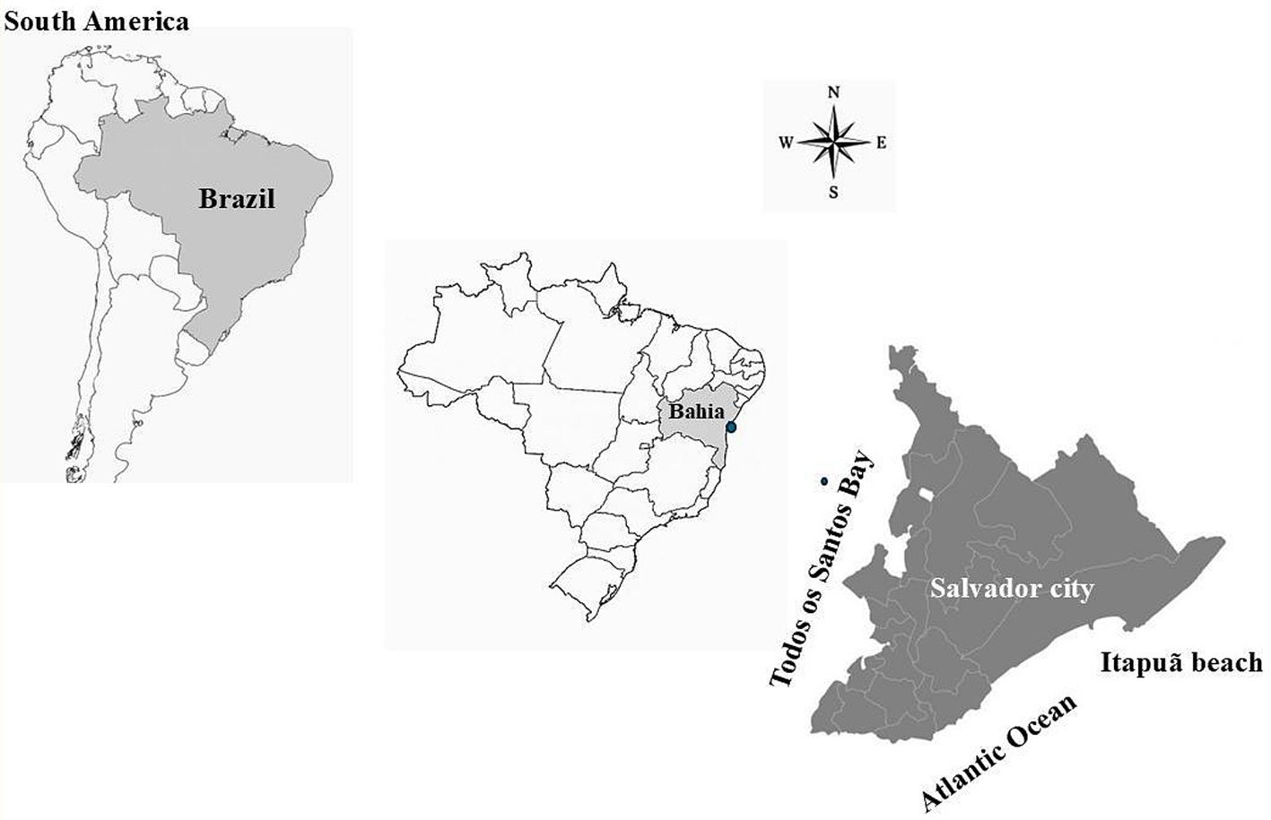
Using the macroalgae biomass data found in each reef zone, the Kruskal-Wallis test was performed to check whether there was a significant difference between the biomass recorded in the different zones. The Bray-Curtis similarity index was also calculated with the biomass data and Non-metric Multidimensional Scaling (nMDS) was performed using the transformed data. ANOSIM was performed for values in which there was a significant difference between the similarity results. The analyses were carried out using SigmaPlot 12 and Primer V6 software.
The species dominance index is used to assess how much one or a few species stand out in relation to the others within a biological community. It considers the proportion of individuals or the biomass of each species, allowing us to identify which of them exert the greatest influence on the structure and functioning of the ecosystem. The higher the value of the index, the greater the dominance, which indicates that a few species concentrate the majority of the individuals present. On the other hand, lower values reflect a more balanced and diverse community, with a lower concentration of individuals in a few species (Melo, 2008).
Simpson’s dominance index was used, calculated as D = ∑ (ni/N) 2, where ni is the number of individuals of a species and N is the total number of individuals of all species in the community. The value of D varies between 0 and 1, with values close to 1 indicating high dominance, that is, few species dominate the environment, while values close to 0 indicate greater diversity and balanced distribution among species.
The Feldmann index (obtained by dividing the number of species of Rhodophyta by that of Phaeophyceae [R/P]) and the Cheney index (adding the number of species of Rhodophyta to that of Chlorophyta, and dividing this value by the number of browns [R + C/ P]) (Figueiredo et al., 2008).
Results
Fifty-two taxa were identified, 27 (52) belonging to the Rhodophyta, 16 (31) Chlorophyta, and 9 (17) Phaeophyceae (Heterokontophyta). Table 1 presents the taxa, their distribution throughout the 3 zones of the reef and their respective morphotypes.
Among the zones, TP presented the greatest species richness (34) with Rhodophyta as the most representative group, 17 taxa, followed by Chlorophyta (11) and Phaeophyceae (6). Chaetomorpha minima, Gayliella dawsonii, Gracilaria ferox, Lejolisia mediterranea, Ptilothamnion speluncarum, and Stylonema alsidii were unique to this environment. PR was second in terms of species richness, such as Caulerpa chemnitzia, Caulerpa sertularioides, Cladophora corallinicola, Hypnea pseudomusciformis, Hypnea sp. 1, and Melanothamnus gorgoniae only occurred in this region. FR presented the lowest richness among the environments, such as Ceramium corniculatum, Codium taylori, Dictyopteris jamaicensis, Dictyopteris polypodioides, Sphacelaria tribuloides, and Wrangelia argus, all exclusive for the region. However, it is worth highlighting a greater representation of rhodophytes for the protected and FR.
Among the species found, 16 occurred in all regions such as Amansia multifida, Amphiroa anastomosans, Anadyomene stellata, Bryopsis pennata, Colpomenia sinuosa, Crouania attenuata, Dictyopteris delicatula, Dictyosphaeria versluysii, Dictyota mertensii, Gelidiella acerosa, Halimeda opuntia, Jania pedunculata var. adhaerens, Palisada perforata, Phyllodictyon anastomosans, Ulva flexuosa, and Ulva rigida.
Regarding the morphotypes, among the 52 taxa found, 19 were filamentous, 17 cylindrical-corticates, 9 foliaceous, 3 articulated calcareous, 3 encrusting and 1 coriaceous. Cylindrical-corticate algae were well represented in the 3 regions, predominating in the PR, followed by foliaceous algae; in the TP, the filamentous morphotype was the one with the highest representation, followed by cylindrical-corticated and foliaceous ones, the same pattern was observed in the FR.
The diversity of analysis based on the Shannon-Wiener index, showed that the TP is more diverse than the others, followed by the PR, and finally by the FR. Dominance values are inversely proportional to diversity values, which shows that in the FR, there is dominance of one or a few species over the others (Table 2).
In table 3, biomass data and the percentage of contribution of each macroalgae in the zone biomass are presented. The average total biomass of each zone was 108.01 g.m-2 in the FR, 48.83 g.m-2 in tide pool and 474.59 g.m-2 in the PR. The Kruskal-Wallis test showed that no significant differences were found in macroalgal biomass between the three reef zones analyzed (Kruskal-Wallis p = 0.869). However, the ordering of the sampling points according to the presence/absence of macroalgae (Fig. 2) shows the dispersion of samples in the 3 zones, mainly samples from the PR. The ANOSIM analysis (Table 4) shows that there was a significant difference between the FR and the TP, and between the FR and the PR, but there was no significant difference between the PR and the TP. The Feldmann and Cheney indices (Fig. 3) for the 3 reef regions studied were consistent with the flora of tropical and warm temperate regions.
Table 1
List of taxa found in the reef zones on Itapuã beach and their respective morphotypes: PR = Protected Region; TP = Tide Pool; FR = Frontal Region. Morphotypes: FT = filamentous; FC = foliaceous; CC = cylindrical corticates; CR = coriaceous; AC = articulated calcareous; E = encrusting. Presence (+) and absence (–).
| Taxa | PR | TP | FR | Morphotype |
| Chlorophyta | ||||
| Ulvophyceae | ||||
| Bryopsidales | ||||
| Bryopsidaceae | ||||
| Bryopsis pennata J.V. Lamouroux | + | + | + | FT |
| Caulerpaceae | ||||
| Caulerpa chemnitzia (Esper) J.V. Lamouroux | + | – | – | CC |
| C. racemosa (Forsskål) J. Agardh | + | + | + | CC |
| C. sertularioides (S.G. Gmelin) M. Howe | + | – | – | CC |
| Codiaceae | ||||
| Codium taylorii P.C. Silva | – | – | + | CC |
| Halimedaceae | ||||
| Halimeda opuntia (Linnaeus) J.V. Lamouroux | + | + | + | AC |
| Ulva flexuosa Wulfen | + | + | + | FC |
| U. rigida C. Agardh | + | + | + | FC |
| Cladophorales | ||||
| Anadyomenaceae | ||||
| Anadyomene stellata (Wulfen) C. Agardh | + | + | + | FC |
| Boodleaceae | ||||
| Phyllodictyon anastomosans (Harvey) Kraft & M.J. Wynne | + | + | + | FT |
| Cladophoraceae | ||||
| Chaetomorpha minima Collins & Hervey | – | + | – | FT |
| Cladophora corallinicola Sonder | + | – | – | FT |
| C. laetevirens (Dillwyn) Kützing | – | + | + | FT |
| C. vagabunda (Linnaeus) Hoek | + | – | + | FT |
| Siphonocladaceae | ||||
| Dictyosphaeria versluysii Weber Bosse | + | + | + | E |
| Valoniaceae | ||||
| Valonia aegagropila C.Agardh | + | + | – | CC |
| Heterokontophyta | ||||
| Phaeophyceae | ||||
| Dictyotales | ||||
| Dictyotaceae | ||||
| Dictyopteris delicatula J.V. Lamouroux | + | + | + | FC |
| D. jamaicensis W.R. Taylor | – | – | + | FC |
| D. polypodioides (De Candolle) J.V. Lamouroux | – | – | + | FC |
| Dictyota mertensii (C.Martius) Kützing | + | + | + | FC |
| Table 1. Continued | ||||
| Taxa | PR | TP | FR | Morphotype |
| Padina antillarum (Kützing) Piccone | + | + | – | FC |
| Spatoglossum schroederi (C. Agardh) Kützing | – | + | + | FC |
| Ectocarpales | ||||
| Scytosiphonaceae | ||||
| Colpomenia sinuosa (Mertens ex Roth) Derbès & Solier | + | + | + | E |
| Fucales | ||||
| Sargassaceae | ||||
| Sargassum polyceratium Montagne | – | + | + | CR |
| Sphacelariales | ||||
| Sphacelariaceae | ||||
| Sphacelaria tribuloides Meneghini | – | – | + | FT |
| Rhodophyta | ||||
| Florideophyceae | ||||
| Ceramiales | ||||
| Callithamniaceae | ||||
| Crouania attenuata (C. Agardh) J. Agardh | + | + | + | FT |
| Ceramiaceae | ||||
| Ceramium corniculatum Montagne | – | – | + | FT |
| Centroceras clavulatum (C. Agardh) Montagne | + | – | – | FT |
| Gayliella dawsonii (A.B. Joly) Barros-Barreto & F.P. Gomes | – | + | – | FT |
| Ceramothamnion brasiliensis (A.B. Joly) M.J. Wynne & C.W. Schneider | + | – | + | FT |
| Rhodomelaceae | ||||
| Alsidium triquetrum (S.G. Gmelin) Trevisan | – | + | – | CC |
| Amansia multifida J.V. Lamouroux | + | + | + | CC |
| Digenea simplex (Wulfen) C. Agardh | + | + | – | CC |
| Herposiphonia bipinnata M. Howe | – | + | – | FT |
| H. tenella (C. Agardh) Ambronn | – | + | – | FT |
| Melanothamnus gorgoniae (Harvey) Díaz-Tapia & Maggs | + | – | – | FT |
| Palisada perforata (Bory) K.W. Nam | + | + | + | CC |
| Wrangeliaceae | ||||
| Lejolisia mediterranea Bornet | – | + | – | FT |
| Ptilothamnion speluncarum (Collins & Hervey) D.L. Ballantine & M.J. Wynne | – | + | – | FT |
| Wrangelia argus (Montagne) Montagne | – | – | + | FT |
| Corallinales | ||||
| Corallinaceae incrustante | ||||
| Jania pedunculata var. adhaerens (J.V. Lamouroux) A.S. Harvey, Woelkerling & Reviers | + | + | + | AC |
| Corallinaceae incrustante | + | – | + | E |
| Lithophyllaceae | ||||
| Table 1. Continued | ||||
| Taxa | PR | TP | FR | Morphotype |
| Amphiroa anastomosans Weber-van Bosse | + | + | + | AC |
| Gelidiales | ||||
| Gelidiaceae | ||||
| Gelidium capense (S.G. Gmelin) P.C. Silva | + | – | + | CC |
| Gelidiellaceae | ||||
| Gelidiella acerosa (Forsskål) Feldmann & Hamel | + | + | + | CC |
| G. ligulata E.Y. Dawson | + | – | + | CC |
| Gigartinales | ||||
| Cystocloniaceae | ||||
| Hypnea pseudomusciformis Nauer, Cassano & M.C. Oliveira | + | – | – | CC |
| Hypnea sp.1 | + | – | – | CC |
| Gigartinaceae | ||||
| Chondracanthus acicularis (Roth) Fredericq | + | + | – | CC |
| Gracilariales | ||||
| Gracilariaceae | ||||
| Gracilaria ferox J. Agardh | – | + | – | CC |
| Nemaliales | ||||
| Galaxauraceae | ||||
| Galaxaura rugosa (J. Ellis & Solander) J.V. Lamouroux | – | + | + | CC |
| Stylonematophyceae | ||||
| Stylonematales | ||||
| Stylonemataceae | ||||
| Stylonema alsidii (Zanardini) K.M. Drew | – | + | – | FT |
| Total | 33 | 34 | 32 |
Discussion
Rhodophyta was the most representative group in the present study, followed by Chlorophyta and Phaeophyceae. This pattern has been observed in other studies on phytobenthic macroalgal communities as typical on the Brazilian coast (Braga et al., 2014; Costa et al., 2012; Ferreira et al., 2022). It should be noted that rhodophytes tend to dominate the environment in the absence of large brown algae in tropical environments, suggesting that there is competition between algae that use different strata in the phytobenthic community (Figueiredo et al., 2004). Furthermore, studies have confirmed the decline of Phaeophyceae at the same rate that Chlorophyta species have been increasing, which can be attributed to the negative effects of anthropogenic impact on the coastal environment (Oliveira & Qi, 2003; Scherner et al., 2013). Representatives of Phaeophyceae are more sensitive to pollutants (heavy metals and excess organic matter produced by sewage), which can even negatively affect the germination and cell division of these organisms (Kevekordes, 2001). Representatives of Chlorophyta, such as species of Ulva Linnaeus, have the capacity of benefit from contamination by pollutants, being considered opportunistic species (Scherner et al., 2012).
Table 2
Shannon-Wiener Diversity index, dominance and equitability of macroalgae in the intertidal region of Itapuã beach.
| Region | Shannon-Wiener | Dominance | Equability (J’) |
| Frontal Region | 3.466 | 0.0312 | 1 |
| Tide Pool | 3.526 | 0.0294 | 1 |
| Protected Region | 3.497 | 0.0303 | 1 |
The taxa that contributed most to the average biomass of macroalgae found on Itapuã beach were Amphiroa anastomosans, Digenea simplex, Gelidiella acerosa, and Sargassum polyceratium. It has been previously reported that algae with greater structural complexity, such as corticate algae, are better adapted to environments with greater hydrodynamics and luminosity, as this morphotype confers greater resistance to desiccation (Costa et al., 2012; Villaça et al., 2008).
Table 3
Biomass and percentage of contribution of macroalgae species in the constitution of biomass in each of the zones studied: FR = Frontal Region, TP = Tide Pool, and PR = Protected Region. Pi = Percentage of importance.
| Taxa | FR (g.m-2) | Pi | TP (g.m-2) | Pi (%) | PR (g.m-2) | Pi (%) |
| Amphyroa anastomosans | 70.07 | 64.87 | 15.76 | 32.28 | 31.59 | 6.66 |
| Anadyomene stellata | 1.41 | 1.31 | 1.76 | 3.61 | 0.00 | 0.00 |
| Bryopsis pennata | 0.00 | 0.00 | 0.20 | 0.42 | 0.00 | 0.00 |
| Caulerpa racemosa | 1.42 | 1.32 | 0.00 | 0.00 | 0.00 | 0.00 |
| C. sertularioides | 0.00 | 0.00 | 0.00 | 0.00 | 1.11 | 0.23 |
| Centroceras clavulatum | 0.00 | 0.00 | 0.00 | 0.00 | 0.25 | 0.05 |
| Chondracanthus acicularis | 0.00 | 0.00 | 0.00 | 0.00 | 0.00 | 0.00 |
| Cladophora vagabunda | 0.00 | 0.00 | 0.00 | 0.00 | 0.15 | 0.03 |
| Colpomenia sinuosa | 0.16 | 0.15 | 0.08 | 0.15 | 0.00 | 0.00 |
| Dictyopteris delicatula | 5.42 | 5.01 | 5.48 | 11.22 | 0.00 | 0.00 |
| D. jamaicensis | 0.00 | 0.00 | 0.00 | 0.00 | 0.00 | 0.00 |
| Dictyosphaeria versluysii | 0.67 | 0.62 | 0.25 | 0.51 | 0.09 | 0.02 |
| Dictyota mertensii | 0.00 | 0.00 | 0.00 | 0.00 | 1.13 | 0.24 |
| Digenea simplex | 0.00 | 0.00 | 0.97 | 1.98 | 430.92 | 90.80 |
| Gelidiellaceae | 0.00 | 0.00 | 2.00 | 4.09 | 0.00 | 0.00 |
| Gelidium sp. 1 | 0.00 | 0.00 | 0.94 | 1.92 | 0.19 | 0.04 |
| Gelidium sp. 2 | 0.00 | 0.00 | 0.00 | 0.00 | 0.09 | 0.02 |
| Gelidiella acerosa | 14.27 | 13.21 | 5.97 | 12.24 | 2.69 | 0.57 |
| G. ligulata | 0.71 | 0.66 | 0.00 | 0.00 | 0.00 | 0.00 |
| Halimeda opuntia | 0.31 | 0.29 | 2.14 | 4.38 | 0.48 | 0.10 |
| Hypnea sp. 1 | 0.40 | 0.37 | 0.00 | 0.00 | 0.00 | 0.00 |
| Hypnea sp. 2 | 0.00 | 0.00 | 0.00 | 0.00 | 0.00 | 0.00 |
| Jania pedunculata var. adhaerens | 7.60 | 7.03 | 0.00 | 0.00 | 0.27 | 0.06 |
| Lobophora variegata | 0.00 | 0.00 | 0.39 | 0.80 | 0.00 | 0.00 |
| Padina antillarum | 0.00 | 0.00 | 2.26 | 4.64 | 1.15 | 0.24 |
| Palisada perforata | 4.86 | 4.50 | 0.00 | 0.00 | 0.05 | 0.01 |
| Phyllodictyon anastomosans | 0.00 | 0.00 | 0.00 | 0.00 | 0.00 | 0.00 |
| Sargassum polyceratium | 0.00 | 0.00 | 9.69 | 19.85 | 0.00 | 0.00 |
| Spatoglossum schroederi | 0.10 | 0.09 | 0.00 | 0.00 | 0.00 | 0.00 |
| Ulva rigida | 0.63 | 0.58 | 0.83 | 1.69 | 3.55 | 0.75 |
| Valonia aegagropila | 0.00 | 0.00 | 0.11 | 0.22 | 0.86 | 0.18 |
| Total | 108.01 | 48.83 | 474.59 |
The difference found in macroalgae biomass between reef zones can be explained by the hydrodynamics to which they are exposed on the reef, being wave action the main responsible for the spatial distribution of the community on the reef. The movement of waves helps to obtain nutrients, favoring the productivity of macroalgae and thus increasing biomass, however this only applies to those algae that have adaptations to resist the impact of waves, as they are also responsible for removing macroalgae from the substrate (Diez et al., 2003; Hurd et al., 1996; Leigh et al., 1987).
The highest biomasses were found in FR and PR. The FR is constantly submerged and this favors the establishment of algae, as they are submerged for longer, suffer less desiccation and are less exposed to direct sunlight. The lowest biomass values were recorded in the TP, a region that retains water during low tide, however the algae are subjected to intense solar radiation, high salinity and water temperature. The negative effects of these stressors result in lower biomass and also there is less hard substrate for fixation (Costa et al., 2012; Villaça et al., 2010).
Table 4
Results of ANOSIM tests for significance of differences between sample groups based on observed macroalgal species distribution data.
| Reef regions | (Global R= 0.613; significance level = 0.4%) | |
| Region pairs | Statistical R | Level |
| FR, TP | 0.815 | 10 |
| FR, PR | 0.667 | 10 |
| TP, PR | 0.481 | 20 |


The dominance of filamentous, cylindrical-corticate and foliaceous morphotypes was observed, corroborating the model by Orfanidis et al. (2001), which proposes that impacted environments should have a greater abundance of algae with intensely branched (corticated), laminar (foliaceous) and filamentous thallus, characterized by high growth rates and a short life cycle (annual). However, conserved environments would have an abundance of algae with thick thallus (coriaceous), articulated calcareous and encrusting, cacterized by low growth rates and a long life cycle (perennial), which reflected in the low representation of articulated, encrusting and coriaceous calcareous morphotypes. In a study carried out by Nascimento (2013) in Salvador and the North Coast of Bahia, the foliaceous and cylindrical-corticate morphotypes were more representative in both impacted and preserved environments, highlighting the predominance of these morphotypes.
The distribution of algae according to morphofunctional groups reflects the conditions of reef zones, since each taxa has its adaptive characteristics. Cylindrical-cortical algae were well represented in the 3 reef zones, with a predominance in the PR, as this morphology confers greater resistance to desiccation, helping these algae to establish themselves in different environments (Costa et al., 2012; Villaça et al., 2008). Tide pool region was dominated by filamentous algae, morphotype usually associated with benthic communities in early successional stages as they show rapid growth (Braga et al., 2014).
Regarding phytogeography, the Feldmann (F) and Cheney (C) indices found for the different regions of the Itapuã reef characterized the PR and the TP as tropical and the FR as warm temperate, according to the classification proposed by Horta et al. (2001). Factors such as the greater hydrodynamism in the FR may justify this classification in relation to its algal community, since the increase in the number of species of brown algae is noticeable as one approaches the FR. Bouzon et al. (2006), studying floristic and phytogeographic aspects of marine macroalgae in the Bays of Santa Catarina, attributed the variations in the Feldmann and Cheney indices to the exclusion of species of brown algae and the favoring of opportunistic species of red and green algae; in this study, lower values of these indices were recorded in the frontal zones and in the pool zone, where the richness of species of brown algae was greater.
Understanding the composition and structure of phytobenthic communities on the Brazilian coast, as well as on the coast of Bahia is extremely important. Despite the vast coastal extension, there are few studies referring to the algal community structure in intertidal zone as most studies focus on the subtidal zone. Also, most studies on the composition and structure of phytobenthic communities are restricted to the state of Rio de Janeiro. More studies should be carried out along the coast of Bahia to fill the gaps and alternating dry and rainy periods and/or comparing the reef zones of different beaches in the intertidal zone. The results suggest that the Itapuã reefs are in a good state of conservation.
Acknowledgements
CCSN, acknowledges the post-doctoral scholarship to the State University of Southwest Bahia (UESB) – Notice 266/2023.; CCSN, LPC, EMSP, to the Coordination for the Improvement of Higher Education Personnel – Brazil (CAPES), finance code 001; CCS, to the Bahia Research Support Foundation (FAPESB – T.O. B., No. BOL0416/2017) for a scholarship.; JMCN, to the National Council for Scientific and Technological Development (CNPq), Brazil for the research productivity fellowship (308261/2022-4).
References
Altamirano, M., & Nunes, J. M. C. (1997). Contribuciones al macrofitobentos del Município de Camaçari (Bahia, Brasil). Acta Botanica Malacitana, 22, 211–215. https://doi.org/10.24310/abm.v22i0.8639
Amado Filho, G. M., Barreto, M. B. B., Marins, B. V., Felix, C., & Reis, R. P. (2003). Estrutura das comunidades fitobentônicas do infralitoral da Baía de Sepetiba, RJ, Brasil. Revista Brasileira de Botânica, 26, 329–342. https://doi.org/10.1590/s0100-84042003000300006
Amorin, P. R. R., Moura, C. W. N., & Moniz-Brito, K. L. (2008). Estudo morfotaxonômico das espécies de Halimeda, Penicillus e Udotea (Bryopsidales, Chlorophyta) do Recife de Franja da Ilha de Itaparica, Bahia. Anais do XI Congresso Brasileiro de Ficologia & Simpósio Latino-Americano sobre Algas Nocivas. Rio de Janeiro: Museu Nacional. Série Livros.
Barbosa, S. O., Figueiredo, M. A. O., & Testa, V. (2008). Structure and dynamic of benthic communities dominated by macrophytes in praia de Jacaraípe, Espírito Santo, Brazil. Hoehnea, 35, 563–575. https://doi.org/10.1590/S2236-89062008000400008
Barreto, M. B. B., Brasileiro, P. S., Nunes, J. M. C., & Amado-Filho, G. M. (2008). Algas marinhas bentônicas do sublitoral das formações recifais da Baía de Todos os Santos, BA – 1. Novas ocorrências. Hoehnea, 31, 321–330.
Braga, A. C. S., Tâmega, F. T. S., Pedrini, A. G., & Muniz, R. A. (2014). Composição e estrutura da comunidade fitobentônica do infralitoral da praia de Itaipu, Niterói, Brasil: Subsídios para monitoramento e conservação. Iheringia. Série Botânica, 69, 267–276. https://isb.emnuvens.com.br/iheringia/article/view/90
Bouzon, J. L., Salles, J. P., Bouzon, Z., & Horta, P. A. (2006). Aspectos florísticos e fitogeográficos das macroalgas marinhas das baías da ilha de Santa Catarina, SC,Brasil. Insular, 35, 69–84.
Caires, T. A., Costa, I. O., Jesus, P. B. D., Matos, M. R. B. D., Pereira-Filho, G. H., & Nunes, J. M. D. C. (2013). Evaluation of the stocks of Hypnea musciformis (Rhodophyta: Gigartinales) on two beaches in Bahia, Brazil. Brazilian Journal of Oceanography, 61, 65–71. https://doi.org/10.1590/S1679-87592013000100007
Costa-Júnior, O. S., Attrill, M. J., Pedrini, A. G., & De Paula, J. C. (2002). Spatial and seasonal distribution of seaweeds on coral reefs from Southern Bahia, Brazil. Botanica Marina, 45, 346–355. https://doi.org/10.1515/BOT.2002.035
Costa, I. O., Caires, T. A., Pereira-Filho, G. H., & Nunes, J. M. C. (2012). Macroalgas bentônicas associadas a bancos de Hypnea musciformis (Wulfen) J.V. Lamour. (Rhodophyta-Gigartinales) em duas praias do litoral baiano. Acta Botanica Brasilica, 26, 493–507. https://doi.org/10.1590/S0102-33062012000200025
Dawes, C., & Mathieson, A. (2008). The seaweeds of Florida. Gainesville: University of Florida Press.
Diez, I., Santolaria, A., & Gorostiaga, J. M. (2003). The relationship of environmental factors to the structure and distribution of subtidal seaweed vegetation of the western Basque coast (N Spain). Estuarine, Coastal and Shelf Science, 56, 1041–1054. https://doi.org/10.1016/S0272-7714(02)00301-3
Ferreira, S. M. C., Lolis, L. A., Noga, P. M., Affe, H. M. J., & Nunes, J. M. C. (2022). A highly diverse phytobenthic community along a short coastal reef gradient in northeastern Brazil. Universitas Scientiarum, 27, 34–56. https://doi.org/10.11144/Javeriana.SC271.ahdp
Figueiredo, M. A. O., Barreto, M. B. B., & Reis, R. P. (2004). Caracterização das macroalgas nas comunidades marinhas da área de Proteção Ambiental de Cairuçú, Parati, RJ – Subsídios para futuros monitoramentos. Revista Brasileira de Botânica, 27, 11–17. https://doi.org/10.1590/S0100-84042004000100002
Figueiredo, M. A. O., Horta, P.A., Pedrini, A. G., & Nunes, J. M. C. (2008). Benthic marine algae of the coral reefs of Brazil: a literature review. Oecologia Brasiliensis, 12, 259–270. https://doi.org/10.4257/oeco.2008.1202.07
Guiry, M. D., & Guiry, G. M. (2025). AlgaeBase. World-wide electronic publication, University of Galway. Retrieved on February 21, 2025 from: https://www.algaebase.org
Horta, P. A., Amancio, E., Coimbra, C. S., & Oliveira, E. C. (2001). Considerações sobre a distribuição e origem da flora de macroalgas marinhas brasileiras. Hoehnea, 28, 243–265.
Horta, P. A., Salles, J. P., Bouzon, J., Scherner, F., Cabral, D., Bouzon, Z. L. et al. (2008). Composição e estrutura dos fitobentos do infralitoral da Reserva Biológica Marinha do Arvoredo, Santa Catarina, Brasil —implicações para a conservação. Oecologia Brasiliensis, 12, 51–57. https://doi.org/10.4257/oeco.2008.1202.06
Hurd, C. L., Harrison, P. J., & Druehl, L. D. (1996). Effect of seawater velocity on inorganic nitrogen uptake by morphologically distinct forms of Macrocystis integrifolia from wave-sheltered and exposed sites. Marine Biology, 126, 205–214. https://doi.org/10.1007/BF00347445
Kevekordes, K. (2001). Toxicity tests using developmental stages of Hormosira banksii (Phaeophyta) identify ammonium as a damaging component of secondary treated sewage effluent discharged into Bass Strait, Victoria, Australia. Marine Ecology Progress Series, 219, 139–148. https://doi.org/10.3354/meps219139
Leigh, E. G., Paine, R. T., Quinn, J. F., & Suchanek, T. H. (1987). Wave energy and intertidal productivity. Proceedings of the National Academy of Sciences, 84, 1314–1318. https://doi.org/10.1073/pnas.84.5.1314
Littler, D. S., & Littler, M. M. (2000). Caribbean reef plants. An identification guide to the reef plants of the Caribbean, Bahamas, Florida and Gulf of Mexico. Washington D.C.: OffShore Graphics.
Macedo, T. S., Varjão, A. S., Fernandes, L. L., Silva, D. F., Almeida, J. S., Messias, J. C. et al. (2009). Levantamento taxonômico e diversidade das macroalgas marinhas bentônicas da praia da Pituba, Salvador, Bahia. Revista Eletrônica de Biologia, 2, 29–39.
Marins, B. V., Brasileiro, P. A., Barreto, M. B. B., Nunes, J. M. C., Yoneshigue-Valentin, Y., & Amado-Filho, G. M. (2008). Subtidal benthic marine algae of the Todos os Santos Bay, Bahia State, Brazil. Oecologia Brasiliensis, 12, 229–242. https://doi.org/10.4257/oeco.2008.1202.05
Melo, A. S. (2008). O que ganhamos “confundindo” riqueza de espécies e equabilidade em um índice de diversidade? Biota Neotropica, 8, 21–27. https://doi.org/10.1590/s1676-06032008000300001
Muñoz, A. O. M., & Pereira, S. M. B. (1997). Caracterização quali-quantitativa das comunidades de macroalgas nas formações recifais da praia do Cupe Pernambuco, Brasil. Trabalhos Oceanográficos da Universidade Federal do Pernambuco, 25, 93–109. https://doi.org/10.5914/tropocean.v25i1.2731
Nascimento, O. S. (2013). Impactos da urbanização sobre a estrutura, cobertura de morfotipos funcionais e heterogeneidade química das comunidades de algas
recifais (M.Sc. Thesis). Instituto de Biologia, Universidade Federal da Bahia, Salvador.
Nunes, J. M. C. (1998a). Catálogo de algas marinhas bentônicas do Estado da Bahia. Acta Botanica Malacitana, 23, 5–21. https://doi.org/10.24310/abm.v23i0.8547
Nunes, J. M. C. (1998b). Rodofíceas marinhas bentônicas da orla oceânica de Salvador, Estado da Bahia, Brasil. Insula, 49, 27–37.
Nunes, J. M. C. (1999). Phaeophyta da Região Metropolitana de Salvador, Bahia, Brasil (M.Sc. Thesis). Instituto de Biociências, Universidade de São Paulo, São Paulo.
Nunes, J. M. C. (2005a). A família Liagoraceae (Rhodophyta, Nemaliales) no Estado da Bahia, Brasil. Hoehnea, 32, 429–444.
Nunes, J. M. C. (2005b). Rodofíceas marinhas bentônicas do Estado da Bahia, Brasil (Ph.D. Thesis). Instituto de Biociências, Universidade de São Paulo, São Paulo.
Nunes, J. M. C. (2010). Taxonomia morfológica: metodologia de trabalho. In A. G. Pedrini (Org.), Macroalgas: uma introdução à Taxonomia (pp. 53–70). Rio de Janeiro, Rio de Janeiro: Technical Books.
Nunes, J. M. C., & Guimarães, S. M. P. B. (2008). Novas referências de rodofíceas marinhas bentônicas para o litoral brasileiro. Biota Neotrópica, 8, 89–100. https://doi.org/10.1590/S1676-06032008000400008
Nunes, J. M. C., & Guimarães, S. M. P. B. (2009). Primeira referência de plantas gametofíticas em Spermothamnion nonatoi (Ceramiales, Rhodophyta). Rodriguésia, 60, 259–264. https://www.jstor.org/stable/23499987
Nunes, J. M. C., & Guimarães, S. M. P. B. (2010). Morfologia y toxonomía de Scinaia halliae (Scinaiaceae, Rhodophyta) em el litoral de Bahia y Espírito Santo, Brasil. Revista
de Biología Marina y Oceonografía, 45, 159–164. http://dx.doi.org/10.4067/S0718-19572010000100017
Nunes, J. M. C., & Paula, E. J. (2000). Estudos taxonômicos do gênero Padina Adanson (Dictyotaceae – Phaeophyta) no litoral do Estado da Bahia, Brasil. Acta Botanica Malaci-
tana, 26, 21–43. https://doi.org/10.24310/abm.v25i0.8470
Nunes, J. M. C., & Paula, E. J. (2001). O gênero Dictyota Laumouroux (Dictyotaceae – Phaeophyta) no litoral do Estado da Bahia, Brasil. Acta Botanica Malacitana, 26, 5–18. https://doi.org/10.24310/abm.v26i0.7375
Nunes, J. M. C., & Paula, E. J. (2002). Composição e distribuição das Phaeophyta nos Recifes da Região Metropolitana de Salvador, Bahia, Brasil. Iheringia, 57, 113–130.
Nunes, J. M. C., & Paula, E. J. (2004a). Chnoosporaceae, Scytosiphonaceae, Sporochnaceae e Sphacelariaceae (Phaeophyta) no Estado da Bahia, Brasil. Biotemas, 17, 7–28.
Nunes, J. M. C., & Paula, E. J. (2004b). Estudos taxonômicos de Ectocarpaceae e Ralfsiaceae (Phaeophyta) da Região Metropolitana de Salvador, Ba, Brasil. Acta Biologica Leopoldensia, 26, 37–50.
Nunes, J. M. C., & Paula, E. J. (2006). O gênero Dictyopteris J.V.Lamour. (Dictyotaceae – Phaeophyta) no estado da Bahia, Brasil. Hidrobiológica, 16, 251–258. https://hidro
biologica.izt.uam.mx/index.php/revHidro/article/view/1036
Nunes, J. M. C., Santos, A. C. C., & Santana, L. C. (2005). Novas ocorrências de algas marinhas bentônicas para o Estado da Bahia, Brasil. Iheringia Série Botânica,60,
99–106. https://isb.emnuvens.com.br/iheringia/article/view/209
Oliveira, E. C., & Qi, Y. (2003). Decadal changes in a polluted bay as seen from its seaweed flora: the case of Santos Bay in Brazil. AMBIO: A Journal of the Human Environment, 32, 403–405. https://doi.org/10.1579/0044-7447-32.6.403
Orfanidis, S., Panayotidis, P., & Stamatis, N. (2001). Ecological evaluation of transitional and coastal waters: a marine benthic macrophytes-based model. Mediterranean Marine Science, 2, 45–65. https://doi.org/10.12681/mms.266
Pedrini, A. G. (2013). Macroalgas (ocrófitas multicelulares) marinhas do Brasil. Rio de Janeiro, Rio de Janeiro: Technical Books.
Scherner, F., Barufi, J. B., & Horta, P. A. (2012). Photosynthetic response of two seaweed species along an urban pollution gradient: evidence of selection of pollution-tolerant species. Marine Pollution Bulletin, 64, 2380–2390. https://doi.org/10.1016/j.marpolbul.2012.08.012
Scherner, F., Horta, P. A., De Oliveira, E. C., Simonassi, J. C., Hall-Spencer, J. M., Chow, F. et al. (2013). Coastal urbanization leads to remarkable seaweed species loss and community shifts along the SW Atlantic. Marine Pollution Bulletin, 76, 106–115. https://doi.org/10.1016/j.marpolbul.2013.09.019
Steneck, R. S., & Dethier, M. N. (1994). A functional group approach to the structure of algal-dominated communities. Oikos, 69, 476-498. http://dx.doi.org/10.2307/3545860
Villaça, R., Yoneshigue-Valentin, Y., & Boudouresque, C. F. (2008). Estrutura da comunidade de macroalgas do infralitoral do lado exposto da ilha de Cabo Frio (Arraial do Cabo, RJ). Oecologia Brasiliensis, 12, 206–221. https://doi.org/10.4257/oeco.2008.1202.03
Villaça, R., Carvalhal-Fonseca, A., Jensen, V. K., & Knoppers, B. (2010). Species composition and distribution of macroalgae on Atol das Rocas, Brazil, SW Atlantic. Botanica Marina, 53, 113–122. https://doi.org/10.1515/BOT.2010.013
Zar, J. H. (2010). Biostatistical analysis. Upper Saddle River, New Jersey: Prentice Hall International.

Panmictic population of the pollinating moth Tegeticula baja(Lepidoptera: Prodoxidae), across the distribution of its plant hosts
Población panmíctica de la polilla polinizadora Tegeticula baja (Lepidoptera: Prodoxidae) a lo largo de la distribución de sus plantas hospederas
Maria Clara Arteaga a, *, C. Rocio Alamo-Herrera a, Anna Darlene van der Heiden a, b, Nicole Sicaeros-Samaniego a
a Centro de Investigación Científica y de Educación Superior de Ensenada, Departamento de Biología de la Conservación,
Carr. Tijuana-Ensenada 3918, Zona Playitas, 22860 Ensenada, Baja California, Mexico
b Uppsala University, Department of Medical Biochemistry and Microbiology, Hursagatan 3, 752 37, Uppsala, Sweden
*Corresponding author: arteaga@cicese.mx (M.C. Arteaga)
Received: 14 March 2025; accepted: 24 July 2025
Abstract
Ecological interactions and demographic history shape the genetic diversity of populations. Tegeticula baja is the specialist pollinator of different Yucca hosts in the Baja California Peninsula, a region that experienced changes in habitat distribution during the Pleistocene. To assess the effects of host specificity and historical changes in habitat configuration, we i) analyzed the genetic structure of moth populations associated with 3 different Yucca plant species, ii) identified signatures of historical demographic changes, and iii) reconstructed the past potential distribution of T. baja at different periods. We genotyped the COI of 128 moths from 39 locations and estimated genetic diversity, population structure, and demographic history. We found an overall haplotype diversity of 0.708 and a nucleotide diversity of 0.0015. Moth populations associated with the 3 hosts exhibited similar diversity levels, with no evidence of genetic structure. These findings suggest that ecological associations with different host plants do not drive T. baja diversification. Instead, its demographic history has played a more significant role in shaping the levels and the distribution of the genetic diversity.
Keywords: Ecological interaction; Genetic diversity; Historical demography; Insect-plant association; Population structure; Yucca
Resumen
Las interacciones ecológicas y la historia demográfica moldean la diversidad genética de las poblaciones. Tegeticula baja es una polinizadora especialista de diferentes yuccas hospederas en la península de Baja California, una región que experimentó cambios en la distribución de los hábitats durante el Pleistoceno. Para evaluar los efectos de la especificidad del huésped y los cambios históricos en la configuración de los hábitats, i) analizamos la estructura genética de las poblaciones de polillas asociadas a distintos hospederos, ii) identificamos señales de cambios demográficos históricos y iii) reconstruimos su distribución potencial en el pasado. Genotipificamos el COI de 128 polillas de 39 localidades y estimamos la diversidad genética, la estructura poblacional y la historia demográfica. Encontramos una diversidad haplotípica global de 0.708 y una diversidad nucleotídica de 0.0015. Las poblaciones de polillas asociadas a las 3 especies de plantas mostraron niveles de diversidad similares, sin evidencia de estructura genética. Estos hallazgos sugieren que la asociación ecológica con diferentes plantas huésped no impulsa la diversificación de T. baja. En cambio, su historia demográfica ha desempeñado un papel más importante en la configuración de su diversidad genética.
Palabras clave: Interacciones ecológicas; Diversidad genética; Historia demográfica; Asociación planta-insecto; Estructura poblacional; Yucca
Introduction
The ecological interaction between pollinator insects and their host plants plays a crucial role in shaping the distribution and genetic diversity of the species involved, influencing processes such as natural selection, genetic drift, and gene flow among populations (Futuyma, 2000; Gloss et al., 2013, 2016). Additionally, other factors, such as geographic distance (e.g., Driscoe et al., 2019) and demographic history shaped by past climatic changes (e.g., Liu et al., 2016; Smith et al., 2011), can influence the amount of genetic variation within populations and its spatial distribution.
Moths of the genus Tegeticula Zeller are specialist pollinators of the genus Yucca Linnaeus, maintaining an obligate mutualism (Engelmann, 1872; Pellmyr, 2003). Generally, each Tegeticula species pollinates a single Yucca species. However, few moth species pollinate multiple Yucca species (Althoff et al., 2006, 2012). During the flowering period, adult moths emerge and mate within Yucca flowers. The female uses specialized mouthparts to collect pollen and transfer it to other flowers. Upon arrival, she inserts her ovipositor into the ovary to lay her eggs. After, she deposits the pollen onto the flower’s stigma, ensuring fertilization and fruit development, from which the larvae will feed on a small portion of the seeds (Engelmann, 1872; Pellmyr, 2003). This obligate interaction between yucca and yucca moths influences the gene flow, facilitating differentiation and diversification processes in both pollinators and host plants (Arteaga et al., 2020; Leebens-Mack & Pellmyr, 2004; Leebens-Mack et al., 1998)
Yucca plants and yucca moths are distributed across North America (Pellmyr et al., 2008). This region has experienced changes in habitat distribution due to Pleistocene climatic fluctuations, which have impacted the genetic diversity and structure of both Yucca populations and their pollinators (Alemán et al., 2024; Arteaga et al., 2020; De la Rosa et al., 2020; Smith et al., 2011). In the Baja California Peninsula (BCP), Mexico, Tegeticula baja Pellmyr is an endemic moth species distributed from the central to the southern part of the peninsula. This moth pollinates 2 endemic Yucca species and their hybrid populations, which exhibit an allopatric distribution: Yucca valida Brandegee occurs in the arid ecosystems of the Central Desert and the northern Magdalena Plains, hybrid populations are found in the southern Magdalena Plains (Arteaga et al., 2020), and Y. capensis Lenz is located in the tropical dry forest of southern BCP (Lenz, 1998; Pellmyr et al., 2008; Turner et al., 1995).
The flowering phenology of these endemic Yucca species and their hybrid populations is asynchronous and influenced by water availability. Yucca valida blooms from April to July (Turner et al., 1995), hybrid populations flower in August and September, and Y. capensis blooms from September to October (Arteaga et al., 2015; Lenz, 1998). The asynchronous flowering limits the temporal coexistence of moths from different populations, as each group responds to the floral signals of its host plant. Additionally, these moths exhibit short-distance dispersal (Álamo-Herrera et al., 2022). Consequently, the temporal availability of floral resources and the limited dispersal of these pollinators may contribute to genetic structuring among populations across their distribution.
Given the obligate interaction between pollinators and plants, we hypothesize that distinct genetic lineages of T. baja are associated with each host Yucca species, influenced by geographic distances and asynchronous flowering. Additionally, considering historical habitat changes in the BCP (Dolby et al., 2015), we expect an impact on the species’ demographic history. Specifically, we i) examined the genetic structure among moth populations associated with each Yucca species and their hybrids, ii) identified signals of historical population changes, and iii) determined how the distribution of suitable conditions for the species has changed over time. This study will contribute to a better understanding of how ecological interactions and historical environmental changes shape the genetic diversity of pollinating moths in the Yucca-Tegeticula mutualism.
Materials and methods
We visited 75 localities where the endemic yuccas and their hybrids were found (Fig. 1A). We collected 3 to 5 fruits from at least 5 plants per locality. We dissected the fruits and examined them for the presence of T. baja larvae, which are typically found among the seeds. We stored the larvae in 96% ethanol and preserved them at -80 °C. We collected a total of 128 moth larvae from 39 of the 75 localities (Fig. 1A), including 16 sites of Yucca valida (N = 49), 8 of Y. capensis (N = 39), and 15 of hybrid plants (N = 40).
We used 20 mg of larval tissue for DNA extraction following the commercial kit “Qiagen DNeasy Blood & Tissue Kit” protocol. We amplified a fragment of the Cytochrome Oxidase subunit I (COI) marker using primers S1461 (5’-ACAATTTATCGCCTAAACTTCAGCC-3’) and A2302 (5’-CTACAAATCCTAATAATCCATTG-3’; Smith et al., 2009). The PCR mixture consisted of 5 μl of buffer (1X), 2 μl of MgCl (2 mM), 0.4 μl of dNTPs (0.6 mM), 0.2 μl of Taq polymerase (1U), 1 μl of each primer (0.4 mM each), 3 μl of DNA, and 12.4 μl of molecular-grade water, for a total reaction volume of 25 μl. Thermocycler conditions were: initial denaturation at 95 °C for 3 min, 35 cycles of denaturation at 94 °C for 30 s, annealing at 48 °C for 45 s, extension at 72 °C for 1 min, and a final elongation at 72 °C for 1 min. We verified the amplification quality using 1% agarose gels. PCR products were sequenced by SeqXcel (www.seqxcel.com). We also tested protocols for amplifying the nuclear EF1α gene and 9 nuclear microsatellites previously used in other species of the same genus (Drummond et al., 2010; Smith et al., 2008); however, amplifications were unsuccessful.
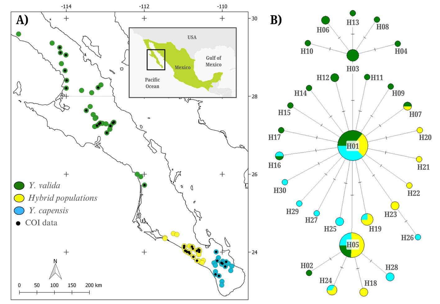
We visualized and edited COI sequences using MEGA X 4.0 and aligned them with MUSCLE (Tamura et al., 2007). We estimated the genetic diversity for the complete dataset and separately for individuals collected in locations from Y. valida, Y. capensis, and the hybrid Y. valida × Y. capensis using DNAsp (Rozas et al., 2003). We calculated the number of polymorphic sites (PS), number of haplotypes (H), haplotype diversity (h), and nucleotide diversity (π). To explore genealogical relationships, we constructed a haplotype network using the Median-Joining method in NETWORK 5.0 (Bandelt et al., 1999). Finally, to assess genetic structure among moths associated with different host plants, we implemented an analysis of molecular variance (AMOVA) using Arlequin (Excoffier et al., 2005).
We assessed the demographic history of T. baja using 3 methods. First, we conducted Tajima’s D test using DNAsp (Rozas et al., 2003). Negative values indicate population expansion, while positive values suggest population reduction (Nakamura et al., 2018). Second, we performed a mismatch distribution analysis in Arlequin, where an unimodal distribution suggests population expansion, while a multimodal distribution indicates a stable population size (Rogers & Harpending, 1992). Finally, we conducted a Bayesian Skyline Plot (BSP) analysis (Drummond et al., 2005) using BEAST 2.6.0 (Bouckaert et al., 2014). As input data, we used the commonly reported nucleotide substitution rate for COI in arthropods (1.77% divergence per lineage per million years; Papadopoulou et al., 2010), a strict molecular clock, and the HKY substitution model defined in JmodelTest2 (Darriba et al., 2012). We ran 100 million steps, sampling every 10,000 generations in the MCMC method. We calculated the effective sample size (ESS) value and constructed the BSP using TRACER 1.7 (Rambaut et al., 2018).
Table 1
Genetic diversity of Tegeticula baja based on the mitochondrial COI marker. The table includes the host plant, sample size (N), number of polymorphic sites (PS), number of haplotypes (H), haplotype diversity (h), and nucleotide diversity (π).
| Host yucca plant | N | PS | H | h | π |
| Yucca valida | 49 | 14 | 17 | 0.733 | 0.0016 |
| Hybrid populations | 40 | 9 | 10 | 0.750 | 0.0015 |
| Yucca capensis | 39 | 11 | 11 | 0.617 | 0.0012 |
We built species distribution models to assess changes in the geographic distribution of suitable conditions for Tegeticula baja and to support the interpretation of its genetic diversity and demographic history estimates. We considered 4 time periods: present (years 1970-2000), mid-Holocene (6,000 years ago), Last Glacial Maximum (22,000 years ago), and Last Interglacial (120,000 – 140,000 years ago). We constructed the models using the 75 sampling points obtained in this study, the 19 bioclimatic variables from the WorldClim 2.1 database (Fick & Hijmans, 2017), and the MAXENT software (Phillips et al., 2006), with 80% of the data used for training and 20% for validation. We configured 2,000 iterations and 10 replicates. The model evaluation included the area under the curve (AUC) and binomial probabilities, where an AUC > 0.9 reflects excellent predictive capacity.

Results
The alignment of 128 sequences resulted in 767 bp with 27 polymorphic sites, defining 30 haplotypes (NCBI ID: PX127684-PX127713; Fig. 1B). The overall haplotype diversity was moderate (h = 0.708), and nucleotide diversity was low (π = 0.0015). Moth populations associated with the 3 host plants exhibited similar diversity levels (Table 1). The haplotype network indicated that haplotypes were closely related, and that the most abundant haplotype was widely distributed among the 3 moth populations pollinating different host plants (Fig. 1B). The AMOVA revealed that the variance among moths associated with different host plants was low and not significant (Fst = 0.011, p = 0.13). In contrast, most variation was found within populations.
Since no signs of genetic structure were detected, demographic analyses and niche modeling were conducted considering all individuals as a panmictic population. Demographic analyses provided evidence of a historical population expansion. Tajima’s D test showed significant negative values (D = -2.27970, p < 0.01), and the mismatch analysis distribution was unimodal (Fig. 2A). Consistently, the BSP analysis suggested a population expansion beginning approximately 25,000 years ago (Fig. 2B).
The species distribution models, with high predictive power (AUC > 0.9), revealed historical changes in the extent and distribution of environmentally suitable areas for T. baja (Fig. 3). During the Last Interglacial (120 ka), the distribution was limited to 2 areas, one in the central and other in the southern regions of the peninsula. During the Last Glacial Maximum (22 ka) and the mid-Holocene (6 ka), an expansion occurred in both regions. Finally, in the present period (1970-2000), the potential distribution of suitable conditions for these moths is observed to be continuously present along the western portion of the peninsula, connecting the central and southern regions.
Discussion
In the obligate mutualism between Yucca plants and Tegeticula moths, the distribution of feeding and oviposition resources provided by host plants determines the presence of moths in the landscape. In this study, we evaluated the genetic structure of Tegeticula baja populations associated with different Yucca species with allopatric distributions. Contrary to our expectations, we found a single panmictic population of pollinator moths throughout its geographic range. Additionally, we detected signals of historical demographic expansion. This suggests that the ecological association with different hosts is not driving the diversification of this species and that its historical demography has played a more relevant role in the distribution of its genetic diversity.
The genetic structure of a species is influenced by multiple factors, such as dispersal capacity, the intensity of ecological interactions, and the climatic history of the areas it inhabits (Driscoe et al., 2019; Futuyma, 2000; Smith et al., 2011). Specifically, T. baja has a limited dispersal distance per generation, and only 1 generation per year (~ 42 m; Álamo-Herrera et al., 2022); its host plants have a discontinuous distribution in the current landscape, and they also exhibit asynchronous flowering (Arteaga et al., 2020; Lenz, 1998; Turner et al., 1995). Together, these factors suggested that we could find genetic structure among moth populations associated with different Yucca species. However, we did not observe significant genetic differentiation. It is possible that the age of origin of its host plants and changes in the distribution of suitable habitat conditions could partially explain this pattern.

The divergence between the 2 endemic Yucca species of the BCP is estimated to have occurred approximately 500,000 years ago (Alemán et al., 2024). The formation of hybrid populations is even a more recent event, proposed to have occurred during the Pleistocene, around 21,000 years ago, when favorable climatic conditions allowed the co-occurrence of Y. valida and Y. capensis in the same region (Arteaga et al., 2020). This period of change in host plant distribution likely also influenced the distribution of the moth Tegeticula baja. Species distribution models and demographic analyses support this, indicating a population expansion beginning around 25,000 years ago, followed by a stabilization phase approximately 3,000 years ago. These historical changes in habitat configuration likely shaped the demographic history of the moth, reducing the potential for genetic divergence across its range due to alternating periods of population isolation and secondary contact. Although the current distribution of host plants is fragmented, the slow generational turnover of T. baja, with 1 generation per year, suggests that insufficient time has passed for genetic drift to produce detectable genetic structure.
The phylogeographic pattern of Tegeticula baja does not exhibit genetic structuring associated with host plant identity, which contrasts with that of other Tegeticula species, where genetic differentiation is correlated with either geographic distance or Yucca host species. For example, T. yucasella exhibits high genetic differentiation associated with geographic distance and interactions with different Yucca species (Leebens-Mack & Pellmyr, 2004). Similarly, T. maculata, the pollinator of Hesperoyucca Engelmann, exhibits genetic clades associated with the biogeographic history of its region (Althoff et al., 2007; Segraves & Pellmyr, 2001). Although all these studies, including ours, used the same mitochondrial marker (COI subunit), we did not detect genetic differentiation in our samples. These differences between our findings and previous reports may be related to the spatial scale, which is much larger in the study of T. yucasella, and to the time of origin and biogeographic history of the host plants in the case of T. maculata (Segraves & Pellmyr, 2001).
The levels of genetic diversity detected in the panmictic population of T. baja were moderate. In particular, moths associated with Y. valida exhibited a higher number of haplotypes, possibly due to their larger geographic range (Fig. 1A). The overall nucleotide diversity was low (π = 0.0015), falling below values reported for other species in the genus, such as T. antithetica and T. synthetica (π = 0.004 and 0.005, respectively; Smith et al., 2008). This pattern of low genetic diversity observed in T. baja may be related to the historical demographic growth detected in this species. A similar pattern was reported in the panmictic population of the parasitoid wasp Digonogastra sp., which interacts with 2 Tegeticula species in the BCP (π = 0.002; Álamo-Herrera et al., 2024). This supports the idea that the levels and distribution of genetic variation in these moths are more related to their historical demography than to their ecological interactions.
In conclusion, integrating genetic data with species distribution models allows us to understand how the climatic history of the BCP has influenced the distribution of genetic diversity and demographic changes in this species. Since the moths’ life cycle depends on Yucca flowering, which in turn responds to precipitation, climate change is likely to affect the population dynamics of these insects. Periods of extreme drought, such as those occurring in recent decades in the peninsula, may impact moth demography and exacerbate a population decline. Future studies focusing on the ecology and evolution of Prodoxus species associated with Yucca and Hesperoyucca in this region could enhance our understanding of the hidden diversity within this group and complement existing information on the northern species (Smith & Leebens-Mack, 2024).
Acknowledgements
The authors are grateful to Lita Castañeda and Mario Salazar for their help with laboratory analysis, technical support, and assistance in the fieldwork. They also thank Alberto López Alemán for his valuable assistance in improving the English language of the manuscript. This study was supported financially by Secretaría de Ciencia, Humanidades, Tecnología e Innovación (Secihti) (CB-2014-01-238843, infra-2014-1-226339). The Rufford Foundation also provided financial support for a part of this study (RSG 13704-1) and the Jiji Foundation. The authors thank the Associate Editor and the anonymous reviewers for their valuable comments. The authors declare no conflicts of interest.
References
Álamo-Herrera, C. R., Arteaga, M. C., Bello-Bedoy, R., & Rosas-Pacheco, F. (2022). Pollen dispersal and genetic diversity of Yucca valida (Asparagaceae), a plant involved in an obligate pollination mutualism. Biological Journal of the Linnean Society, 136, 364–374. https://doi.org/10.1093/biolinnean/blac031
Álamo-Herrera, C. R., Arteaga, M. C., & Bello-Bedoy, R. (2024). Genetic diversity and phenotypic variation in a parasitoid wasp involved in the yucca – yucca moth interaction. Revista Mexicana de Biodiversidad, 95, e955461. https://doi.org/10.22201/ib.20078706e.2024.95.5461
Alemán, A., Arteaga, M. C., Gasca-Pineda, J., & Bello-Bedoy, R. (2024). Divergent lineages in a young species: the case of Datilillo (Yucca valida), a broadly distributed plant from the Baja California Peninsula. American Journal of Botany, 111, e16385. https://doi.org/10.1002/ajb2.16385
Althoff, D. M., Segraves, K. A., Leebens-Mack, J., & Pellmyr, O. (2006). Patterns of speciation in the yucca moths: parallel species radiations within the Tegeticula yuccasella species complex. Systematic Biology, 55, 398–410. https://doi.org/10.1080/10635150600697325
Althoff, D. M., Svensson, G. P., & Pellmyr, O. (2007). The influence of interaction type and feeding location on the phylogeographic structure of the yucca moth community associated with Hesperoyucca whipplei. Molecular Phylogenetics and Evolution, 43, 398–406. https://doi.org/10.1016/j.ympev.2006.10.015
Althoff, D. M., Segraves, K. A., Smith, C. I., Leebens-Mack, J., & Pellmyr, O. (2012). Geographic isolation trumps coevolution as a driver of yucca and yucca moth diversification. Molecular Phylogenetics and Evolution, 62, 898–906. https://doi.org/10.1016/j.ympev.2011.11.024
Arteaga, M. C., Bello-Bedoy, R., León-de la Luz, J. L., Delgadillo, J., & Domínguez, R. (2015). Phenotypic variation of flowering and vegetative morphological traits along the distribution for the endemic species Yucca capensis (Agavaceae). Botanical Sciences, 93, 765–770. https://doi.org/10.17129/botsci.214
Arteaga, M. C., Bello-Bedoy, R., & Gasca-Pineda, J. (2020). Hybridization between yuccas from Baja California: Genomic and environmental patterns. Frontiers in Plant Science, 11, 685. https://doi.org/10.3389/fpls.2020.00685
Bandelt, H. J., Forster, P., & Röhl, A. (1999). Median-joining networks for inferring intraspecific phylogenies. Molecular Biology and Evolution, 16, 37–48. https://doi.org/10.1093/oxfordjournals.molbev.a026036
Bouckaert, R., Heled, J., Kühnert, D., Vaughan, T., Wu, C. H., Xie, D. et al. (2014). BEAST 2: a software platform for Bayesian evolutionary analysis. Plos Computational Biology, 10, e1003537. https://doi.org/10.1371/journal.pcbi.1003537
Darriba, D., Taboada, G. L., Doallo, R., & Posada, D. (2012). jModelTest 2: more models, new heuristics and high-performance computing. Nature Methods, 9, 772. https://doi.org/10.1038/nmeth.2109
De la Rosa-Conroy, L., Gasca-Pineda, J., Bello-Bedoy, R., Eguiarte, L. E., & Arteaga, M. C. (2020). Genetic patterns and changes in availability of suitable habitat support a colonisation history of a North American perennial plant. Plant Biology, 22, 233–242. https://doi.org/10.1111/plb.13053
Dolby, G. A., Bennett, S. E. K., Lira-Noriega, A., Wilder, B. T., & Munguia-Vega, A. (2015). Assessing the geological and climatic forcing of biodiversity and evolution surrounding the Gulf of California. Journal of the Southwest, 57, 391–455.
Driscoe, A. L., Nice, C. C., Busbee, R. W., Hood, G. R., Egan, S. P., & Ott, J. R. (2019). Host plant associations and geography interact to shape diversification in a specialist insect herbivore. Molecular Ecology, 28, 4197–4211. https://doi.org/10.1111/mec.15220
Drummond, A. J., Rambaut, A., Shapiro, B. E. T. H., & Pybus, O. G. (2005). Bayesian coalescent inference of past population dynamics from molecular sequences. Molecular Biology and Evolution, 22, 1185–1192. https://doi.org/10.1093/molbev/msi103
Drummond, C. S., Xue, H. J., Yoder, J. B., & Pellmyr, O. (2010). Host-associated divergence and incipient speciation in the yucca moth Prodoxus coloradensis (Lepidoptera: Prodoxidae) on three species of host plants. Heredity, 105, 183–196. https://doi.org/10.1038/hdy.2009.154
Engelmann, G. (1872). The flower of yucca and its fertilization. Bulletin of the Torrey Botanical Club, 3, 33.
Excoffier, L., Laval, G., & Schneider, S. (2005). Arlequin (version 3.0): an integrated software package for population genetics data analysis. Evolutionary Bioinformatics Online, 2005, 47–50. https://doi.org/10.1177/117693430500100003
Fick, S. E., & Hijmans, R. J. (2017). WorldClim 2: new 1-km spatial resolution climate surfaces for global land areas. International Journal of Climatology, 37, 4302–4315. https://doi.org/10.1002/joc.5086
Futuyma, D. J. (2000). Some current approaches to the evolution of plant–herbivore interactions. Plant Species Biology, 15, 1–9. https://doi.org/10.1046/j.1442-1984.2000.00029.x
Gloss, A. D., Dittrich, A. C. N., Goldman-Huertas, B., & Whiteman, N. K. (2013). Maintenance of genetic diversity through plant–herbivore interactions. Current Opinion in Plant Biology, 16, 443–450. https://doi.org/10.1016/j.pbi.2013.06.002
Gloss, A. D., Groen, S. C., & Whiteman, N. K. (2016). A genomic perspective on the generation and maintenance of genetic diversity in herbivorous insects. Annual Review of Ecology, Evolution, and Systematics, 47, 165–187. https://doi.org/10.1146/annurev-ecolsys-121415-032220
Leebens-Mack, J., Pellmyr, O., & Brock, M. (1998). Host specificity and the genetic structure of two yucca moth species in a yucca hybrid zone. Evolution, 52, 1376–1382. https://doi.org/10.1111/j.1558-5646.1998.tb02019.x
Leebens-Mack, J., & Pellmyr, O. (2004). Patterns of genetic structure among populations of an oligophagous pollinating Yucca moth (Tegeticula yuccasella). Journal of Heredity, 95, 127–135. https://doi.org/10.1093/jhered/esh025
Lenz, L. W. (1998). Yucca capensis (Agavaceae, Yuccoideae), a new species from Baja California Sur, Mexico. Cactus and Succulent Journal, 70, 289–296.
Liu, S., Jiang, N., Xue, D., Cheng, R., Qu, Y., Li, X. et al. (2016). Evolutionary history of Apocheima cinerarius (Lepidoptera: Geometridae), a female flightless moth in northern China. Zoologica Scripta, 45, 160–174. https://doi.org/10.1111/zsc.12147
Nakamura, H., Teshima, K., & Tachida, H. (2018). Effects of cyclic changes in population size on neutral genetic diversity. Ecology and evolution, 8, 9362–9371. https://doi.org/10.1002/ece3.4436
Papadopoulou, A., Anastasiou, I., & Vogler, A. P. (2010). Revisiting the insect mitochondrial molecular clock: the mid-Aegean trench calibration. Molecular Biology and Evolution, 27, 1659–1672. https://doi.org/10.1093/molbev/msq051
Pellmyr, O. (2003). Yuccas, yucca moths, and coevolution: a review. Annals of the Missouri Botanical Garden, 90, 35–55.
Pellmyr, O., Balcazar-Lara, M., Segraves, K. A., Althoff, D. M., & Littlefield, R. J. (2008). Phylogeny of the pollinating yucca moths, with revision of Mexican species (Tegeticula and Parategeticula; Lepidoptera, Prodoxidae). Zoological Journal of the Linnean Society, 152, 297–314. https://doi.org/10.1111/j.1096-3642.2007.00361.x
Phillips, S. J., Anderson, R. P., & Schapire, R. E. (2006). Maximum entropy modeling of species geographic distributions. Ecological Modelling, 190, 231–259. https://doi.org/10.1016/j.ecolmodel.2005.03.026
Rambaut, A., Drummond, A. J., Xie, D., Baele, G., & Suchard, M. A. (2018). Posterior summarization in Bayesian phylogenetics using Tracer 1.7. Systematic Biology, 67, 901–904. https://doi.org/10.1093/sysbio/syy032
Rogers, A. R., & Harpending, H. (1992). Population growth makes waves in the distribution of pairwise genetic differences. Molecular Biology and Evolution, 9, 552–569. https://doi.org/10.1093/oxfordjournals.molbev.a040727
Rozas, J., Sánchez-Del Barrio, J. C., Messeguer, X., & Rozas, R. (2003). DnaSP, DNA polymorphism analyses by the coalescent and other methods. Bioinformatics, 19, 2496–2497. https://doi.org/10.1093/bioinformatics/btg359
Segraves, K. A., & Pellmyr, O. (2001). Phylogeography of the yucca moth Tegeticula maculata: the role of historical biogeography in reconciling high genetic structure with limited speciation. Molecular Ecology, 10, 1247–1253. https://doi.org/10.1046/j.1365-294X.2001.01275.x
Smith, C. I., Godsoe, W. K., Tank, S., Yoder, J. B., & Pellmyr, O. (2008). Distinguishing coevolution from covicariance in an obligate pollination mutualism: asynchronous divergence in Joshua tree and its pollinators. Evolution, 62, 2676–2687. https://doi.org/10.1111/j.1558-5646.2008.00500.x
Smith, C. I., Drummond, C. S., Godsoe, W., Yoder, J. B., & Pellmyr, O. (2009). Host specificity and reproductive success of yucca moths (Tegeticula spp. Lepidoptera: Prodoxidae) mirror patterns of gene flow between host plant varieties of the Joshua tree (Yucca brevifolia: Agavaceae). Molecular Ecology, 18, 5218–5229. https://doi.org/10.1111/j.1365-294X.2009.04428.x
Smith, C. I., Tank, S., Godsoe, W., Levenick, J., Strand, E., Esque, T. et al. (2011). Comparative phylogeography of a coevolved community: concerted population expansions in Joshua trees and four yucca moths. Plos One, 6, e25628. https://doi.org/10.1371/journal.pone.0025628
Smith, C. I., & Leebens-Mack, J. H. (2024). 150 Years of coevolution research: evolution and ecology of yucca moths (Prodoxidae) and their hosts. Annual Review of Entomology, 69, 375–391. https://doi.org/10.1146/annurev-ento-022723-104346
Tamura, K., Dudley, J., Nei, M., & Kumar, S. (2007). MEGA4: molecular evolutionary genetics analysis (MEGA) software version 4.0. Molecular Biology and Evolution, 24, 1596–1599. https://doi.org/10.1093/molbev/msm092
Turner, R. M., Bowers, J. E., & Burgess, T. L. (1995). Sonoran Desert plants: an ecological atlas. Tucson: University of Arizona Press.

Prorocentrum lima complex associated with macrophytes at two eastern boundary upwelling sites: Estero de Urías Lagoon (Mexico) and Paracas Bay (Peru)
Complejo Prorocentrum lima asociado a macrofitas en dos sitios de afloramiento de borde oriental: laguna Estero de Urías (México) y bahía de Paracas (Perú)
Tomasa Cuellar-Martinez a, *, Ana Carolina Ruiz-Fernández a, Joan Albert Sanchez-Cabeza a, Arturo Aguirre-Velarde b, Haydeé Felícita López-Cabanillas b, Jorge Tam c,
Sonia Sánchez c, François Colas d
a Universidad Nacional Autónoma de México, Instituto de Ciencias del Mar y Limnología, Unidad Académica Mazatlán, Capitán Joel Montes Camarena s/n, Cerro del Vigía, 82040 Mazatlán, Sinaloa, Mexico
b Universidad Nacional Agraria La Molina, Facultad de Pesquería, Av. La Molina s/n, La Molina, Lima, Peru
c Instituto del Mar del Perú, Esquina Gamarra y General Valle s/n, Chucuito Callao, Lima, Peru
d Institut de Recherche pour le Développement (IRD), Laboratoire LOPS, Institut Universitaire Européen de la Mer (IUEM), 29280 Plouzané, France
*Corresponding author: tcuellar@ola.icmyl.unam.mx (T. Cuellar-Martinez)
Received: 20 November 2024; accepted: 17 September 2025
Abstract
Benthic or epibenthic dinoflagellates (EDs) are a potential risk to the environment and human health due to the production of toxins by some species. This study explored for the first time the presence of EDs mainly associated with macrophytes (macroalgae and seagrass) at 2 sites influenced by upwellings: Estero de Urías Lagoon (EUL), at the entrance of the Gulf of California, and Paracas Bay (PB), on the southern Peruvian coast. Prorocentrum lima complex was present at low abundances: ≤ 25 cells g-1 wet weight in EUL and ≤ 867 cells g-1 wet weight in PB. It was recorded in a wide range of temperatures from 22.2 to 31.6 °C in EUL and from 18.0 to 22.2 °C in PB. Despite its low abundance, monitoring the EDs community is essential to detect changes in the distribution patterns of harmful species in the context of climate change.
Keywords: Macroalgae; Caulerpa; Artificial substrate; California Current; Humboldt Current
Resumen
Los dinoflagelados epibentónicos (DE) representan un riesgo potencial al ambiente y a la salud del ser humano debido a la producción de toxinas por parte de algunas especies. En este estudio, se exploró por primera vez la presencia de DE principalmente asociados a macrofitas (macroalgas y pastos marinos) en 2 sitios con influencia de afloramientos: laguna Estero de Urías (LEU), localizado en la entrada del golfo de California y la bahía de Paracas (BP) en la costa sur de Perú. El complejo Prorocentrum lima estuvo presente con bajas abundancias: ≤ 25 células g-1 peso húmedo en LEU y ≤ 867 células g-1 peso húmedo en BP. La especie se registró en un amplio intervalo de temperatura de 22.2 a 31.6 °C en LEU y de 18.0 a 22.2 °C en BP. A pesar de las bajas abundancias encontradas, el monitoreo de la comunidad de DE es importante para detectar cambios en los patrones de distribución de las especies nocivas en un contexto de cambio climático.
Palabras clave: Macroalgas; Caulerpa; Sustrato artificial; Corriente de California; Corriente de Humboldt
Introduction
Benthic or epibenthic dinoflagellates (EDs) are common in shallow waters. They are frequently attached to many substrate types, such as algal turf, macroalgae, rocks, coral rubble, sand, or seagrasses (Honsell et al., 2013; Yong et al., 2018). Although they prefer substrate attachment, the vegetative cells of free-living species are flagellated and are fully capable of detachment and motility (Durán-Riveroll et al., 2019). The excessive growth of these species, particularly the toxigenic ones, can produce benthic harmful algal blooms, and toxins can be transferred along the food web; in humans, consumption of contaminated seafood with these toxins can cause diarrhetic shellfish poisoning (DSP) or ciguatera fish poisoning (Berdalet et al., 2016).
Although EDs have a high relative cell abundance and diversity in subtropical and tropical waters, they are found globally, including in temperate, sub-arctic, and polar environments (Álvarez et al., 2022; Tester et al., 2010). In recent decades, evidence suggests a shift in biogeographical distribution patterns for some species (Gobler et al., 2017; Tester et al., 2020), such as Gambierdiscus,previously considered tropical or sub-tropical. Recent studies have shown that it is well established in temperate areas such as Korea, Japan, New Zealand, Australia, the northern Gulf of Mexico, and the Mediterranean Sea (Chinain et al., 2021). Furthermore, there is concern that floating plastics in the ocean can act as global vectors for transporting algal cells and transferring toxins along marine food webs (do Prado-Leite et al., 2022).
In Mexico, about 60 species from 18 EDs genera have been identified. The species that form dense benthic blooms with potentially harmful consequences are Prorocentrum rhathymum, Blixaea quinquecornis, and Amphidinium cf. carterae (Okolodkov et al., 2022). In South America, 31 EDs taxa have been reported (Mafra et al., 2023). The most frequent and widespread species was the P. lima complex (Mafra et al., 2023). On the Peruvian coast, the cold coastal waters of the Humboldt Current System could restrict the presence of these species (Durán-Riveroll et al., 2019). The P. lima complex has been frequently observed over the past ~ 50 years, though studies have primarily focused on the planktonic community (Mafra et al., 2023).
Benthic microalgae are expected to benefit from climate change conditions, such as warmer waters and changes in marine current patterns, which could promote their invasive colonization and range of expansion (Tester et al., 2010). Estero de Urías Lagoon (EUL) and Paracas Bay (PB) host harbors with high levels of activity (i.e., the harbors of Mazatlán and San Martín, respectively), which may represent a potential risk since ballast waters remain a vector for the introduction of non-native and potentially harmful aquatic species (Lee et al., 2021). This study aimed to explore the EDs associated with macrophytes in Estero de Urías Lagoon, Mazatlán (Mexico), and Paracas Bay, Pisco (Peru), and the environmental variables associated with the presence of these species.
Materials and methods
Estero de Urías Lagoon (EUL; 23.2° N) is located at the entrance to the Gulf of California (Fig. 1) and covers an area of 18 km2 with water depths of 1-3 m except in the navigation channel where it is up to 13 m (Montaño-Ley et al., 2008). It is surrounded by the industrialized city and harbor of Mazatlán (Raygoza-Viera et al., 2014). It is influenced by seasonal coastal upwelling events (Herrera-Becerril et al., 2022). EUL does not receive continuous freshwater, for which it exhibits an inverse estuarine circulation, and during the warmest months high salinity occurs in the upper lagoon (Cardoso-Mohedano et al., 2018).
The climate in the area is warm and humid, with a mean annual temperature of 21.4-29.6 °C (1951-2017) and a mean annual precipitation of 372 mm (SMN, 2024). EUL is an anthropized coastal lagoon affected by urban development, shrimp farming, and discharges of domestic, industrial, and wastewater (Hernández-Cornejo & Ruiz-Luna, 2000; Méndez, 2002). The Mazatlán harbor is the second largest on the Mexican Pacific coast, and in 2023 it received almost 500,000 cruise ship passengers from the largest cruise ships navigating the globe (API, 2024).
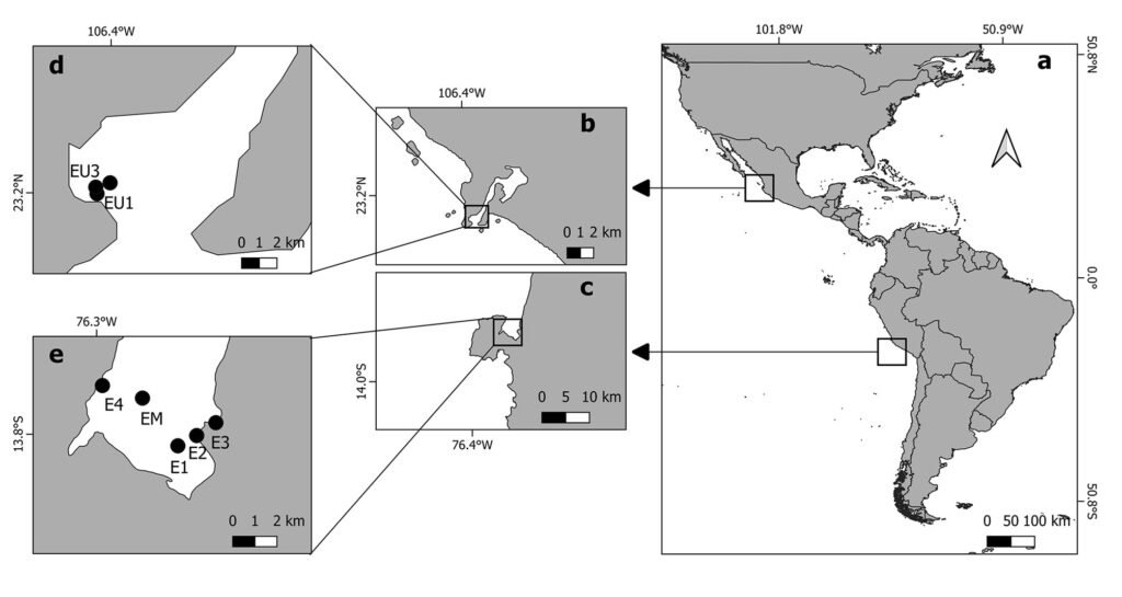
Figure 1. a, Map of the study sites; b, d, sampling sites in Estero de Urías (EU1, EU2, EU3), Mexico; c, e, Paracas Bay (E1, E2, E3, E4, EM), Peru.
Paracas Bay (PB; 13.8° S) is located in Pisco, off South-Central Peru (Fig. 1), with an area of 30 km2 and < 15 m of depth (Merma-Mora et al., 2024). The southern part of the bay is included in the Paracas National Reserve (Sernanp, 2019). It is influenced by one of the main upwelling cells of the highly productive Peruvian Upwelling System (Chávez et al., 2008). PB is seasonally influenced by river discharge, and monthly averages range from 0.7 to 282 m3 s−1, with the higher values in austral summer (Cuellar-Martinez et al., 2023).
The climate in the region is arid, with an average annual rainfall of 1.83 mm and air temperatures ranging from 15 to 22 °C (Reyes, 2009). Anthropogenic activities around the bay include artisanal and industrial fishing, tourism, bay scallop Argopecten purpuratus aquaculture, fish processing industries, non-metallic minerals, and guano extraction (Reyes, 2009). The Terminal Portuario General San Martín, the country’s third most important port for cargo traffic (APN, 2018), is in the surroundings.
The most abundant macrophytes were collected manually or by diving and placed in polypropylene bags; the macrophyte masses ranged from 5 to 342.2 g in wet weight. The 3 sampling sites at EUL were close to the lagoon mouth, where a greater diversity of macroalgae species is found (Ochoa-Izaguirre et al., 2002). The sites were located in a total area of 0.01 km2 with fish cage cultures (~ 8 m depth). The most abundant macroalgae attached to the floating cage frames were collected monthly between August and November 2018 and in January, February, April, and June 2019. A total of 25 samples were collected, including species of Gracilaria sp., Hynea sp., Sargassum sp., Padina sp., Grateloupia sp., and Gelidium sp. In general, 1 to 4 samples were collected per sampling station. In addition, between August and October 2018, artificial substrates consisting of rectangular pieces (3 x 33 cm) of fiberglass screen fixed on a rigid frame were used (Jauzein et al., 2016). The artificial substrates were collected using scissors. For retrieval, 24 hours after installation, the substrate was cut on one side and carefully placed into a plastic bottle filled with 250 ml of ambient seawater. Then, the other side of the substrate was cut and placed inside the bottle, which was capped underwater (Jauzein et al., 2016).
In PB, the most abundant macrophytes, such as Caulerpa filiformis, Chondracanthus chamissoi, and Ruppia maritima were collected at 5 sites during June and November 2021, and April 2022. The sites were shallow (~ 1 m depth), whereas E1 and EM were 5 m and 10 m deep, respectively. A total of 24 samples were obtained. Additionally, surface water was sampled daily in E1 to evaluate the presence of EDs in the water (cells L-1), and HOBO data loggers (Onset UA-001-64) recorded surface and bottom temperatures every 20 minutes.
Environmental parameters (temperature, salinity, dissolved oxygen, and chlorophyll a) were measured in both PB and EUL using EXO (YSI) multiparameter sondes. In EUL, the chlorophyll a sensor was calibrated using rhodamine standards according to the manufacture’s guidelines (YSI Inc., 2014), allowing chlorophyll a concentrations to be expressed in absolute units (μg L⁻¹). In contrast, no calibration was performed in PB; thus, chlorophyll a values are reported in RFU (relative fluorescence units), reflecting the raw sensor response. Although not directly comparable to absolute concentrations, RFU values are widely used to identify temporal patterns in relative chlorophyll a concentrations (Foster et al., 2022). In the EUL, measurements were taken near the sampling sites (1-2 km) at stations 3 and 4 for the coastal observatory of global change in Mazatlán (Fig. 1 in Sanchez-Cabeza et al., 2019) and at station E1 for PB.
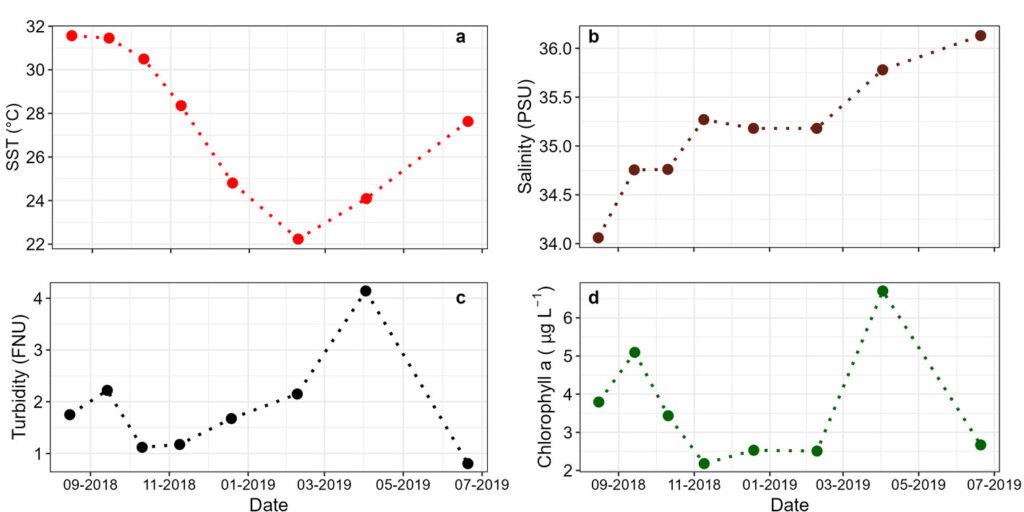
Figure 2. Mean values of the sea surface temperature (SST in °C). a) Salinity (PSU; b), turbidity (in nephelometric turbidity units, NTU); c) chlorophyll a concentration (in µg L-1; d) in the Estero de Urías Lagoon, at the entrance of the Gulf of California.
In the laboratory, the bags with macrophytes and bottles with artificial substrates were vigorously agitated for 2 minutes. The suspension was filtered through sieves with 250 µm, 150 µm, and 20 µm mesh to remove larger particles. The fraction retained in the 20 µm sieve was concentrated and transferred to a vial of 50 ml filled with seawater filtered through Whatman GF/F filters (nominal pore size ~ 0.7 µm), and preserved with 1% acidic Lugol’s iodine fixative. The EDs counting was performed on 3 replicate subsamples from the same macrophyte sample, using a Sedgwick-Rafter chamber in an optical microscope (LM Leica DMR, Wetzlar, Germany) with 200× magnification. Cell abundances were reported as cells per g w.w. of macrophyte (Reguera et al., 2011). The reported uncertainty is the standard deviation of the mean of 3 replicate counts.
The Shapiro test confirmed that species densities were not normally distributed. Therefore, Kruskal-Wallis one-way ANOVA and Dunn’s multiple comparison post hoc tests were used to assess whether abundances and environmental variables exhibited significant variations during the study period. The significance level (α) was set at < 0.05. All analyses and plots were performed with R version 2024.04.2 (R Core Team, 2024).
Results
Estero de Urías Lagoon
During the study period, the sea surface temperature (SST) varied from 22.2 to 31.6 °C, salinity from 34.0 to 36.1, turbidity from 0.8 to 4.1 NTU, and chlorophyll a from 2.2 to 6.7 mg L-1. The highest SST was observed in August-September, 2018 (Fig. 2).
No EDs were observed attached to the artificial substrates in the EUL. Macroalgae were not found in EU2 in November 2018 and June 2019. Dinoflagellates on the EUL macroalgae belonged to the genus Prorocentrum; the highest abundances corresponded to P. micans (Supplementary material; Fig. S1). Prorocentrum lima complex was frequently observed in the samples, with abundances ranging from 0 to 78±45 cells g-1. No significant differences in the abundances were observed between seasons or among stations (Fig. 3a, b). Spearman’s correlation between the abundances of EDs and environmental variables was not significant.
Paracas Bay
During the study period, temperatures were from 14.1 to 22.2 °C. The sea surface and bottom temperatures were significantly higher in autumn (surface temperatures: 18.0-22.2 °C; bottom temperatures: 17.5-21.6 °C) than in summer and spring (surface temperatures: 14.5-22.1 °C; bottom temperatures: 14.1-19.7 °C; Fig. 4a). In the 3 seasons, the surface temperatures were significantly higher than the bottom temperatures. When the P. lima complex was observed in the water column and associated with macrophytes (May 14-Jun 04), SST ranged from 18.0 to 22.2 °C. Chlorophyll a ranged from 0.45 to 7.12 RFU. The highest values were observed in autumn, while spring and summer values were similar. The salinity varied between 34.4 and 35.2, with higher values in autumn than in spring and summer (4b).
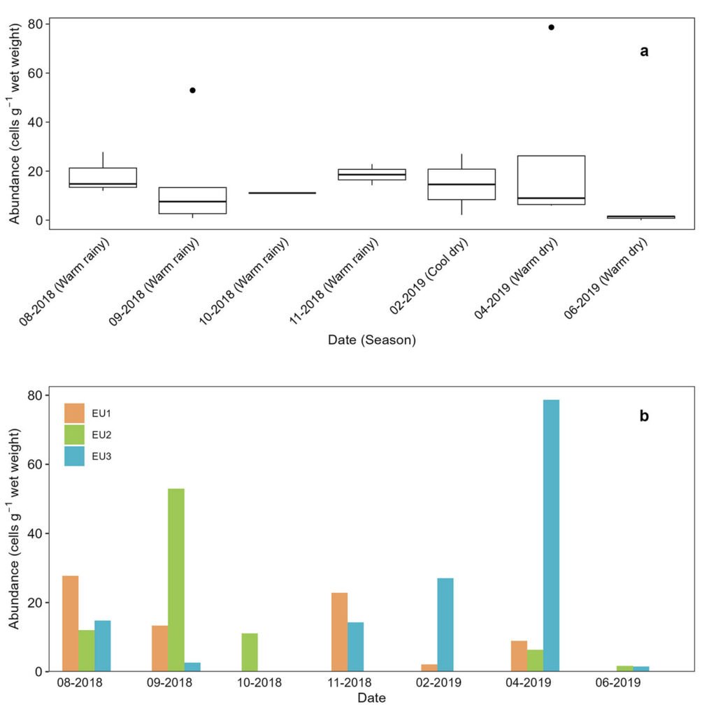
Figure 3. a) Abundance of the Prorocentrum lima complex, with seasons indicated in parentheses. Boxplots show the median (horizontal line), the interquartile range (the difference between the third and first quartile; box). Whiskers extend to values within 1.5 times the interquartile range, and data beyond this range are shown as outliers (dots); b, total abundance by station sites in the Estero de Urías Lagoon, located at the entrance of the Gulf of California.
In Paracas Bay, EDs were absent during most of the study period, and the P. lima complex was detected only in the austral autumn (June 2-4, 2021; Fig. 5, Table 1) with the highest abundances (867±172 cells g-1 in station E3). The P. lima complex was attached mostly to C. filiformis (Table 1).
According to the high-frequency monitoring of Prorocentrum species in surface water, P. micans was a common dinoflagellate in austral autumn and summer, and its abundances were from 40 to 1,840 cells L-1 (Supplementary material; Fig. S2). The P. lima complex was observed only in the austral autumn with a maximum abundance (1,360 cell L-1) on May 14, and between May 17 and June 01, its abundances were ≤ 280 cells L-1 (Fig. 4c).
Discussion
Artificial substrates have been successfully used for quantifying and monitoring EDs, particularly in sheltered, shallow, and subtidal sites (Tester et al., 2022). The lack of EDs attached to the artificial substrates in EUL is likely related to the low abundance of these organisms and the lagoon’s turbulent hydrodynamics. Low abundances of EDs were also observed associated with macroalgae. These results agree with observations from the coast of Tonga in an area exposed to high wave action, where Argyle (2018) detected low abundances of Gambierdiscus cells in association with macrophytes, but the artificial substrate failed to collect them. In contrast, Gambierdiscus concentrations were high on natural and artificial substrates deployed at sheltered, shallow, and subtidal sites. Despite EUL mouth having the highest macroalgae diversity (Ochoa-Izaguirre et al., 2002), it is not a sheltered zone. It is influenced by the tidal regime since the energy available for water circulation is primarily provided by tidal pumping, with tidal velocities of up to 0.60 m s-1 at the main channel (Montaño-Ley et al., 2008). The EDs can be attached by coating mucus or can live freely within the macroalgae interstices, so the turbulence and currents make them vulnerable to cell dispersal. They are mainly found in areas with low to moderately low energy environments (Foden et al., 2005).
Table 1
Abundance of Prorocentrum species in Paracas Bay in the austral autumn.
| Species | Date | Season | Station | Macrophyte species | Abundance (cells g wet weight)* |
| Prorocentrum lima complex | 2021-06-02 | Autumn | E3 | Caulerpa filiformis | 861±172 |
| Prorocentrum lima complex | 2021-06-02 | Autumn | E3 | Caulerpa filiformis | 250±17 |
| Prorocentrum lima complex | 2021-06-02 | Autumn | E3 | Caulerpa filiformis | 13±3 |
| Prorocentrum micans | 2021-06-02 | Autumn | E3 | Caulerpa filiformis | 6±5 |
| Prorocentrum lima complex | 2021-06-04 | Autumn | E3 | Chondracanthus chamissoi +Ulva sp. | 0 |
| Prorocentrum lima complex | 2021-06-04 | Autumn | E3 | Red algae | 0 |
| Prorocentrum lima complex | 2021-06-04 | Autumn | E3 | Red algae | 0 |
| Prorocentrum lima complex | 2021-06-04 | Autumn | E4 | Chondracanthus chamissoi | 1±1 |
| Prorocentrum lima complex | 2021-06-04 | Autumn | E4 | Ruppia marítima | 5±5 |
| Prorocentrum lima complex | 2021-06-04 | Autumn | E4 | Ruppia maritima | 5±2 |
* Abundances represent the average of 3 independent counts performed on the same sample. Values are reported as the mean ± standard deviation.
Among the Prorocentrum species associated with macrophytes in this study, only P. lima complex is recognized as a benthic species (Okolodkov et al., 2022), and it is the first time that P. lima complexis reportedattached to macrophytes in EUL and PB. This cosmopolitan taxon is widely distributed in South America (Mafra et al., 2023). Although low abundances were observed in PB, P. lima has been recorded in the water column with abundances of up to 4.5×10⁴ cells L-1 (Cuellar-Martinez et al., 2023). Caulerpa filiformis is the most representative species in the macroalgae assemblage of PB (Olivas-Valverde, 2013), and the highest abundances of P. lima complex were observed on this species. Although information about the toxicity of P. lima complex is not available in strains from PB or EUL, reports worldwide reveal that all studied P. lima strains produce toxins related to DSP, such as okadaic acid, and several strains produce dinophysistoxins-1 (DTX1; Nishimura et al., 2020). Thus, monitoring this species on different substrates is relevant.
The presence of P. lima complex in both the water column and on macroalgae in Paracas Bay coincided with the highest temperatures recorded during the study period. Aissaoui et al. (2014) mentioned that this species appears to be eurythermal and euryhaline, as it grows over a wide interval of temperatures and salinities. In this work, P. lima complex was observed over a wide range of temperatures (18.0-31.6 °C), suggesting a remarkable ecological plasticity and ability to colonize diverse niches. Although P. lima complex was previously observed in PB at temperatures ranging from 15 to 25 °C (Mafra et al., 2023), in this study it was detected during autumn, when the highest temperatures reached 17.5-22.2 °C. Aquino-Cruz et al. (2018) highlighted the importance of temperature on cell growth rates, toxin levels, and photosynthetic efficiency. They determined that the optimum growth of P. lima strains from the United Kingdom occurred at 15-25 °C, with an increment in the production of okadaic acid at 15 °C.
Temperatures also affect the range of species distribution. It is expected that warmer temperatures associated with climate change could benefit harmful benthic dinoflagellate species, expanding their geographical distribution range (Tester et al., 2020). Another factor associated with distribution expansion is the artificial introduction of discharged ballast ship water (Park et al., 2021). The sampling period of this study limits the potential for making strong extrapolations regarding the temporal dynamics of the DEs and their ecological dynamics. Nevertheless, the detection of DEs with potential toxin production is a relevant finding that highlights the need for longer-term monitoring to better understand their ecological dynamics and potential harmful implications for environmental health and human activities.
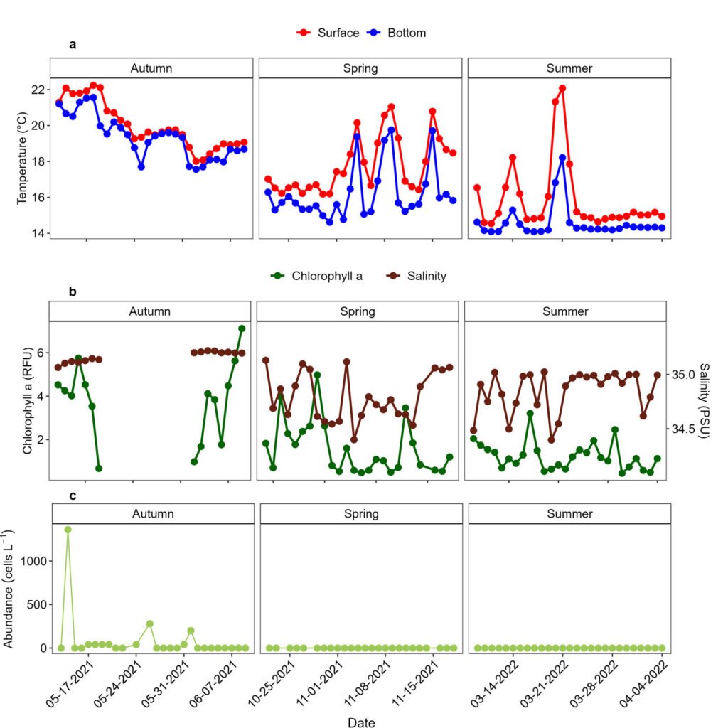
Figure 4. Surface and bottom temperatures (in °C). a) Surface salinity (PSU) and chlorophyll a (in relative fluorescence units, RFU; b), and seasonal abundances of Prorocentrum lima complex in surface waters (c) at the E1 station in Paracas Bay, Peru.
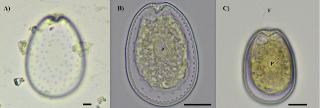
Figure 5. Vegetative cells of Prorocentrum lima complex collected from Paracas Bay, Peru, observed under light microscopy. A) Surface focus on a vegetative cell showing the pore pattern, B) cell showing pyrenoid (P), C) cell showing pyrenoid and flagellu. Scale bar: 10 µm.
The epibenthic dinoflagellate community was explored at 2 sites influenced by upwellings: Estero de Urías Lagoon, at the entrance to the Gulf of California, and Paracas Bay, off south-central Peru. The Prorocentrum lima complex was commonly found with low abundances, mainly associated with macrophytes in Estero de Urías Lagoon and sporadically detected in Paracas Bay (mainly on Caulerpa filiformis). In the water column of Paracas Bay, the P. lima complex was observed during the period with the highest recorded temperature in the study, suggesting potential environmental influences. These initial findings highlight the need for long-term studies with higher temporal resolution and increased detection frequency to better understand the environmental relationships of the benthic dinoflagellate at the studied sites. Given the known production of diarrhetic shellfish toxins by P. lima, its possible sensitivity to climate-related changes, and the anthropogenic pressures present in both study areas —such as intense marine traffic— further monitoring and multidisciplinary research, including toxicological, physiological, and molecular studies, are strongly recommended to assess the potential risks posed by P. lima to marine ecosystems and public health.
Acknowledgments
This work was supported by UNAM ICML (#347), IAEA-RLA/7014 and 7028, Project Concytec – World Bank 05-2019-FONDECYT-BM. This is a contribution to the Marine-Coastal Research Stressors Network for Latin America and the Caribbean (REMARCO) www.remarco.org and to the IRN DEXICOTROP of the Institut de Recherche pour le Développement (IRD). The authors thank M. Rangel, O. López Ramos, M. Fregoso-López, B. Yáñez-Chávez, H. Bojórquez-Leyva, and F. Rioual for the help provided in the fieldwork; R. Alonso-Rodríguez, J. A. Cabello Coral, B. Yáñez-Rivera, for microscopy facilities. F. Ramos-Huamaní and L. H. Pérez-Bernal for the laboratory analyses, and M. Ochoa-Izaguirre for the identification of macroalgae from the Estero de Urías Lagoon.
References
Aissaoui, A., Armi, Z., Akrout, F., & Ben-Hassine, O. K. (2014). Environmental factors and seasonal dynamics of Prorocentrum lima population in coastal waters of the Gulf of Tunis, South Mediterranean. Water Environment Research, 86, 2256–2270. https://doi-org/2443/10.2175/106143014X13975035526266
Álvarez, E. A., Klemm, K., Hoppenrath, M., Cembella, A., John, U., & Karlson, B. (2022). Temporal and spatial distribution of epibenthic dinoflagellates in the Kattegat-Skagerrak, NE Atlantic-Focus on Prorocentrum lima and Coolia monotis. Harmful Algae, 118, 102318. https://doi.org/10.1016/j.hal.2022.102318
API (Administración Portuaria Integral). (2024). Puerto de Mazatlán: plataforma logística integral. Available at https://www.puertomazatlan.com.mx/APIWEB/PRESENTA
TION_APIMAZ.PDF (Accessed May 20 2024).
APN (Autoridad Portuaria Nacional). (2018). Plan Maestro del Terminal Portuario General San Martin. Lima, Peru. Available at: http://webaplicacion.apn.gob.pe/proyecto/wp-
content/uploads/2020/10/Plan-Maestro-Portuario-TP-GENERAL-SAN-MARTIN.pdf (Accessed: March 11, 2024).
Aquino-Cruz, A., Purdie, D. A., & Morris, S. (2018). Effect of increasing sea water temperature on the growth and toxin production of the benthic dinoflagellate Prorocentrum lima. Hydrobiologia, 813, 103–122. https://doi.org/10.1007/s10750-018-3512-4
Argyle, P. A. (2018). The ecology and toxin production of Gambierdiscus and Fukuyoa species from the Pacific (Ph.D. Thesis). University of Canterbury, New Zealand.
Berdalet, E., Fleming, L. E., Gowen, R., Davidson, K., Hess, P., Backer et al. (2016). Marine harmful algal blooms, human health and wellbeing: challenges and opportunities in the 21st century. Journal of the Marine Biological Association of the United Kingdom, 96, 61–91. https://doi.org/10.1017/S0025315415001733
Cardoso-Mohedano, J. G., Lima-Rego, J., Sanchez-Cabeza, J. A., Ruiz-Fernández, A. C., Canales-Delgadillo, J., Sánchez-Flores, E. I. et al. (2018). Sub-tropical coastal lagoon salinization associated to shrimp ponds effluents. Estuarine, Coastal and Shelf Science, 203, 72–79. https://doi.org/10.1016/j.ecss.2018.01.022
Chávez, F. P., Bertrand, A., Guevara-Carrasco, R., Soler, P., & Csirke, J. (2008). The northern Humboldt Current System: Brief history, present status and a view towards
the future. Progress in Oceanography, 79, 95–105. https://doi.org/10.1016/j.pocean.2008.10.012
Chinain, M., Gatti, C. M. I., Darius, H. T., Quod, J. P., & Tester, P. A. (2021). Ciguatera poisonings: A global review of occurrences and trends. Harmful Algae, 102, 101873. https://doi.org/10.1016/j.hal.2020.101873
Cuellar-Martinez, T., Ochoa, A. D. R. H., Sánchez, S., Aguirre-Velarde, A., Ocas, E. O. M., Velasquez, A. M. R. et al. (2023). Abundance and distribution of potentially toxic phytoplankton in aquaculture sites along the Peruvian coast. Journal of Marine Systems, 240, 103865. https://doi.org/10.1016/j.jmarsys.2023.103865
do Prado-Leite, I., Menegotto, A., da Cunha-Lana, P., & Júnior, L. L. M. (2022). A new look at the potential role of marine plastic debris as a global vector of toxic benthic algae. Science of the Total Environment, 838, 156262. https://doi.org/10.1016/j.scitotenv.2022.156262
Durán-Riveroll, L. M., Cembella, A. D., & Okolodkov, Y. B. (2019). A review on the biodiversity and biogeography of toxigenic benthic marine dinoflagellates of the coasts of Latin America. Frontiers in Marine Science, 6, 148. https://doi.org/10.3389/fmars.2019.00148
Foden, J., Purdie, D. A., Morris, S., & Nascimento, S. (2005). Epiphytic abundance and toxicity of Prorocentrum lima populations in the Fleet Lagoon, UK. Harmful Algae, 4, 1063–1074. https://doi.org/10.1016/j.hal.2005.03.004
Foster, G. M., Graham, J. L., Bergamaschi, B. A., Carpenter, K. D., Downing, B. D., Pellerin, B. A. et al. (2022). Field techniques for the determination of algal pigment fluorescence in environmental waters. Principles and guidelines for instrument and sensor selection, operation, quality assurance, and data reporting (No. 1-D10). Virginia: US Geological Survey. https://doi.org/10.3133/tm1D10
Gobler, C. J., Doherty, O. M., Hattenrath-Lehmann, T. K., Griffith, A. W., Kang, Y., & Litaker, R. W. (2017). Ocean warming since 1982 has expanded the niche of toxic algal blooms in the North Atlantic and North Pacific oceans. Proceedings of the National Academy of Sciences, 114, 4975–4980. https://doi.org/10.1073/pnas.1619575114
Hernández-Cornejo, R., & Ruiz-Luna, A. (2000). Development of shrimp farming in the coastal zone of southern Sinaloa (Mexico): operating characteristics, environmental issues, and perspectives. Ocean & Coastal Management, 43, 597–607. https://doi.org/10.1016/S0964-5691(00)00049-1
Herrera-Becerril, C. A., Sanchez-Cabeza, J. A., Sánchez, L. F. Á., Lara-Cera, A. R., Ruiz-Fernández, A. C., Cardoso-Mohedano, J. G. et al. (2022). Statistical identification of coastal hypoxia events controlled by wind-induced upwelling. Continental Shelf Research, 233, 104634. https://doi.org/10.1016/j.csr.2021.104634
Honsell, G., Bonifacio, A., De Bortoli, M., Penna, A., Battocchi, C., Ciminiello, P. et al. (2013). New insights on cytological and metabolic features of Ostreopsis cf. ovata Fukuyo (Dinophyceae): A multidisciplinary approach. Plos One, 8, e57291. https://doi.org/10.1371/journal.pone.0057291
Jauzein, C., Fricke, A., Mangialajo, L., & Lemée, R. (2016). Sampling of Ostreopsis cf. ovata using artificial substrates: optimization of methods for the monitoring of benthic harmful algal blooms. Marine Pollution Bulletin, 107, 300–304. https://doi.org/10.1016/j.marpolbul.2016.03.047
Lee, E. S., Hwang, J., Hyung, J. H., & Park, J. (2021). Detection of the benthic dinoflagellates, Ostreopsis cf. ovata and Amphidinium massartii (Dinophyceae), Using Loop-Mediated Isothermal Amplification. Journal of Marine Science and Engineering, 9, 885. https://doi.org/10.3390/jmse9080885
Mafra, Jr., L. L., Sunesen, I., Pires, E., Nascimento, S. M., Álvarez, G., Mancera-Pineda, J. E. et al. (2023). Benthic harmful microalgae and their impacts in South America. Harmful Algae, 127, 102478. https://doi.org/10.1016/j.hal.2023.102478
Méndez, N. (2002). Annelid assemblages in soft bottoms subjected to human impact in the Urías Estuary (Sinaloa, Mexico). Oceanologica Acta, 25, 139–147. https://doi.org/
10.1016/S0399-1784(02)01193-3
Merma-Mora, L., Colas, F., Cardich, J., Sánchez, S., Flores, E., Lorenzo, A. et al. (2024). Bottom-water hypoxia in the Paracas Bay (Peru, 13.8° S) associated with seasonal and synoptic time scale variability of winds and water stratification. Journal of Marine Systems, 241, 103918. https://doi.org/10.1016/j.jmarsys.2023.103918
Montaño-Ley, Y., Peraza-Vizcarra, R., & Páez-Osuna, F. (2008). Tidal hydrodynamics and their implications for the dispersion of effluents in Mazatlán Harbor: An urbanized shallow coastal lagoon. Water, Air, and Soil Pollution, 194, 343–357. http://dx.doi.org/10.1007/s11270-008-9721-0
Nishimura, T., Uchida, H., Noguchi, R., Oikawa, H., Suzuki, T., Funaki, H. et al. (2020). Abundance of the benthic dinoflagellate Prorocentrum and the diversity, distribution, and diarrhetic shellfish toxin production of Prorocentrum lima complex and P. caipirignum in Japan. Harmful Algae, 96, 101687. https://doi.org/10.1016/j.hal.2019.101687
Ochoa-Izaguirre, M. J., Carballo, J. L., & Páez-Osuna, F. (2002). Qualitative changes in macroalgal assemblages under two contrasting climatic conditions in a subtropical estuary. Botanica Marina, 45, 130–138. https://doi.org/10.1515/BOT.2002.014
Okolodkov, Y. B., Durán-Riveroll, L. M., Band-Schmidt, C. J., Leyva-Valencia, I., Gárate-Lizárraga, I., & Cembella, A. D. (2022). A review on marine benthic dinoflagellates in Mexico. Hidrobiológica, 32, 183–210. https://doi.org/10.24275/uam/izt/dcbs/hidro/2022v32n3/okolodkov
Olivas-Valverde, J. A. (2013). Informe de evaluación e identificación de potenciales riesgos ambientales en flora y fauna en la Bahía de Paracas, provincia de Pisco, departamento de Ica. Organismo de Evaluación y Fiscalización Ambiental. Gobierno de Perú. Available at https://repositorio.oefa.gob.pe/handle/20.500.12788/1214 (Accessed May 28, 2024).
Park, J. S., Li, Z., Kim, H. J., Kim, K. H., Lee, K. W., Youn, J. Y. et al. (2021). First report of the marine benthic dinoflagellate Bysmatrum subsalsum from Korean tidal pools. Journal of Marine Science and Engineering, 9, 649. https://doi.org/10.3390/jmse9060649
Raygoza-Viera, J. R., Ruiz-Fernández, A. C., Ruelas-Inzunza, J., Alonso-Hernández, C., Pérez-Bernal, L. H., & Páez-Osuna, F. (2014). Accumulation and distribution of Hg and 210Pb in superficial sediments from a coastal lagoon in the SE Gulf of California associated with urban-industrial and port activities. Environmental Earth Sciences, 72, 2729–2739. https://doi.org/10.1007/s12665-014-3178-9
R Core Team. (2024). R: a language and environment for statistical computing. R Foundation for Statistical Computing, Vienna, Austria. https://www.R-project.org/
Reguera, B., Alonso, R., Moreira, A., & Méndez, S. (2011). Guía para el diseño y puesta en marcha de un plan de seguimiento de microalgas productoras de toxinas. Proyecto ARCAL RLA 7/014. París, Viena: UNESCO/ OIEA.
Reyes, J. (2009). Paracas, nuestra Reserva. Información básica sobre la Reserva Nacional de Paracas (2ª ed.). Áreas Costeras y Recursos Marinos, [ACOREMA]. http://humboldt.iwlearn.org/es/sitios-piloto/-1/paracas.pdf
Sanchez-Cabeza, J. A., Álvarez Sánchez, L. F., Cardoso-Mohedano, J. G., Escalante-Mancera, E., Díaz-Asencio, M., López-Rosas, H. et al. (2019). A low-cost long-term model of coastal observatories of global change. Journal of Operational Oceanography, 12, 34–46. https://doi.org/10.1080/1755876X.2018.1533723
Sernanp (Servicio Nacional de Áreas Naturales Protegidas). (2019). Reserva Nacional de Paracas. Servicio Nacional de Áreas Naturales Protegidas por el Estado. Available at: https://www.gob.pe/institucion/sernanp/informes-publicaciones/1718991-reserva-nacional-de-paracas (Accessed October 23, 2024).
SMN (Servicio Meteorológico Nacional). (2024). Normales climatológicas Mazatlán 1951-2017. Available at https://smn.cna.gob.mx/tools/RESOURCES/Diarios/25062.txt
Tester, P. A., Feldman, R. L., Nau, A. W., Kibler, S. R., & Litaker, R. W. (2010). Ciguatera fish poisoning and sea surface temperatures in the Caribbean Sea and the West Indies. Toxicon, 56, 698–710. https://doi.org/10.1016/j.toxicon.2010.02.026
Tester, P. A., Litaker, R. W., & Berdalet, E. (2020). Climate change and harmful benthic microalgae. Harmful Algae, 91, 101655. https://doi.org/10.1016/j.hal.2019.101655
Tester, P. A., Litaker, R. W., Soler-Onís, E., Fernández-Zabala, J., & Berdalet, E. (2022). Using artificial substrates to quantify Gambierdiscus and other toxic benthic dinoflagellates for monitoring purposes. Harmful Algae, 120, 102351. https://doi.org/10.1016/j.hal.2022.102351
Yong, H. L., Mustapa, N. I., Lee, L. K., Lim, Z. F., Tan, T. H., Usup, G. et al. (2018). Habitat complexity affects benthic harmful dinoflagellate assemblages in the fringing reef of Rawa Island, Malaysia. Harmful Algae, 78, 56–68. https://doi.org/10.1016/j.hal.2018.07.009
YSI Inc. (2014). EXO Rhodamine WT Smart Sensor Calibration Guide. Available at: https://www.fondriest.com/pdf/ysi_exo_rhodamine_cal.pdf

Vascular epiphyte community of an inland mangrove of Tabasco: composition and similarity with coastal mangroves and adjacent tropical vegetation
Vascular epiphyte community of an inland mangrove of Tabasco: composition and similarity with coastal mangroves and adjacent tropical vegetation
Comunidad epífita vascular de un manglar interior de Tabasco: composición y similitud con manglares costeros y vegetación tropical adyacente
Neil Ebeth Meled Morales-Rodríguez a, *, Carlos Manuel Burelo-Ramos a, José G. García-Franco b, Octavio Aburto-Oropeza c y María Eugenia Molina-Paniagua a
a Universidad Juárez Autónoma de Tabasco, Laboratorio de Manglares Interiores, Carretera Villahermosa-Cárdenas Km. 0.5 s/n, Entronque a Bosques de Saloya, 86150 Villahermosa, Tabasco, Mexico
b Instituto de Ecología, Carretera antigua a Coatepec #351, Col. El Haya, 91073 Xalapa, Veracruz, Mexico
c Scripps Institution of Oceanography, 9500 Gilman Drive, La Jolla, California 92093, USA
*Corresponding author: nemmr@hotmail.com (N.E.M. Morales-Rodríguez)
Received: 13 December 2024; accepted: 23 October 2025
Abstract
El Cacahuate Lagoon, Tabasco, Mexico, is located 170 km from the current coastline and contains an inland mangrove ecosystem, surrounded by remnants of tropical forest. This inland mangrove is the habitat of an epiphyte community whose species composition and relationship with other epiphyte communities are unknown. This study describes the composition of vascular epiphytes associated with this inland mangrove, evaluates their similarity to epiphyte communities in coastal mangroves and adjacent vegetation within a 220 km radius of the study site, using the Jaccard Index and floristic turnover with β-diversity. We hypothesize that the similarity in the composition of the epiphytes of the inland mangrove should be greater with that of nearby forests than with coastal mangroves, since the seeds of forest epiphytes can easily reach the inland mangrove. The epiphyte community of the Cacahuate mangrove comprises 27 species and is more similar to the epiphyte communities of the coastal mangroves of Tabasco. This affinity could be related to the Pleistocene isolation of this mangrove, or to the long-distance dispersal of epiphytes from coastal mangroves.
Keywords: Biodiversity; Floristics; Red mangrove; Rhizophora mangle; Wanha’ Biosphere Reserve
Resumen
La laguna El Cacahuate, Tabasco, México, se localiza a 170 km de la línea costera actual y contiene un ecosistema de manglar interior, rodeado de remanentes de bosque tropical. Este manglar interior es el hábitat de una comunidad epífita cuya composición de especies y su relación con otras comunidades epífitas se desconocen. El presente estudio describe la composición de epífitas vasculares asociadas con este manglar interior, evalúa su similitud con las comunidades epífitas de los manglares costeros y vegetación adyacente en un radio de 220 km del lugar de estudio, utilizando el índice de Jaccard y su recambio florístico con la diversidad ß. Hipotetizamos que la similitud en la composición de las epífitas del manglar interior debería ser mayor con la de los bosques cercanos que con los manglares costeros, ya que las semillas de las epífitas de los bosques pueden llegar fácilmente al manglar interior. La comunidad epífita del manglar del Cacahuate comprende 27 especies y presenta una mayor similitud con las comunidades epífitas de los manglares costeros de Tabasco. Esta afinidad podría estar relacionada con el aislamiento pleistocénico de este manglar, o con la dispersión a larga distancia de las epífitas provenientes de los manglares costeros.
Palabras clave: Biodiversidad; Florística; Mangle rojo; Rhizophora mangle; Reserva de la Biosfera Wanha’
Introduction
Vascular epiphytic plants (henceforth epiphytes) constitute a functional group that develops on woody species. Unlike parasitic plants, epiphytes obtain water and nutrients from the atmosphere, precipitation, and decomposing organic material, rather than relying physiologically on the host (Krömer & Gradstein, 2016). Within epiphytes, 2 main categories are recognized: true epiphytes, which complete their entire life cycle on the host without producing roots that reach the soil, and hemiepiphytes, which in contrast, exhibit a mixed life cycle, since some germinate on the host and later develop roots that reach the ground (primary hemiepiphytes), whereas others begin their growth in the soil and, as they ascend, establish themselves on the host (secondary hemiepiphytes) (Granados-Sánchez et al., 2003; Zotz, 2016). Epiphytes comprise about 10% of the known plant species worldwide (Zotz et al., 2021). In the Neotropics, epiphytes significantly contribute to the overall diversity of the vegetation, as they can represent up to 50% of the vascular flora in some forests (Carmona-Higuita et al., 2025; Kelly et al., 2004; Taylor et al., 1986). Tree species in the low and mountain forests have different structural characteristics (e.g., greater height, dense canopy, and great diversity of bark textures), which combined with particular environmental conditions (e.g., high humidity), allow the presence of a high number of epiphytic species (Ceja-Romero et al., 2008; Flores-Palacios & García-Franco, 2006; Hietz & Hietz, 1995; Krömer et al., 2007, 2014; Martínez-Meléndez et al., 2011; Rzedowski, 1996). In contrast, mangrove forests generally show a low richness of epiphytes (Benzing, 1990; Carmona-Díaz et al., 2014; Zotz & Reuter, 2009; Zimmerman & Olmsted, 1992), which can be attributed to reduced tree diversity and consequently to low structural complexity of the habitat, but mainly due to environmental stress conditions such as the strong winds, waves, and high salinity present in coastal zones (Gómez & Winker, 1991; Jiménez-López et al., 2017; Zotz & Reuter, 2009). However, epiphytes are frequent in mangrove ecosystems, as several species have been recorded in different studies even though the objectives and sampling efforts are directed toward tree species, which are the dominant physiognomic elements (Aksornkoae, 1993; Cach-Pérez et al., 2013; Carmona-Díaz et al., 2014; De Sousa & Colpo, 2017; García-Luna et al 2024; Jiménez-López et al., 2018; Kupec, 2018; Noguera-Savelli et al., 2021; Rahman et al., 2015; Rohani et al., 2020).
Mangrove ecosystems are primarily distributed in tropical and subtropical regions, generally associated with the coast and brackish water bodies (Leal & Spalding, 2021). However, mangrove ecosystems also have been recorded in freshwater wetlands, away from marine influence, known as inland mangroves. The inland mangroves have been reported in many countries worldwide, such as in Australia, Antigua and Barbuda, the Bahamas, Indonesia, and Pakistan, located 15 to 50 km from the coast, and between 6 and 37 m above sea level (Lugo, 1981; Patel, 2014; Patel & Agoramoorthy, 2012; Stoddart et al., 1973; Taylor, 1986; Tripathi et al., 2013; Woodroffe, 1988).
Recently, in Mexico, individuals of Rhizophora mangle, along with another 112 coastal affinity species were reported along the banks of the San Pedro Mártir River and El Cacahuate Lagoon in Tabasco, the latter located almost on the border with Guatemala (Aburto-Oropeza et al., 2021). The presence of this inland mangrove is attributed to the global climatic phenomenon that occurred about 120,000 years ago when an increase in global temperatures caused a rise in sea levels, displacing the coastline inland (Aburto-Oropeza et al., 2021). As the planet cooled, the sea retreated to its current position, leaving mangrove trees dispersed along the riverbanks and creating an isolated mangrove ecosystem in the El Cacahuate Lagoon, 170 km from the Tabasco coast (Aburto-Oropeza et al., 2021).
Currently, the El Cacahuate Lagoon is surrounded by a matrix composed of remnants of evergreen tropical forest belonging to the “Cañón del Usumacinta” Flora and Fauna Protection Zone (Conanp, 2015), fragments of several types of tropical forest, and large areas of land used for livestock and agriculture activities. However, despite this mixed landscape, the hydrophytic vegetation surrounding the water body restricts access to the mangrove, which has resulted in minimal human impact. El Cacahuate mangrove is considered a relict area from the Pleistocene and a refuge for biodiversity due to its high degree of conservation (Aburto-Oropeza et al., 2021). This area together with the adjacent forest areas forms part of a core area of the recently designated Wanha’ Biosphere Reserve (Conanp, 2023a; Semarnat, 2023).
Preliminary surveys indicate the presence of several species of epiphytes along the upper San Pedro River (Aburto-Oropeza et al., 2021). However, in El Cacahuate mangrove the epiphyte species composition and its species similarities to the epiphytic communities of the surrounding vegetation or to the coastal mangroves of Gulf of Mexico are unknown. High epiphyte composition similarity with tropical forest would indicate processes of colonization after the sea retired, while high epiphyte composition with coastal mangroves communities should indicate that species arrived together with the mangrove during the interglacial period.
The aims of this study were to determine the richness and composition of the epiphyte community present in the inland mangrove of El Cacahuate Lagoon, and to assess the floristic similarity of the epiphytes of El Cacahuate with coastal mangroves and adjacent tropical forests. We expect that, given the inland Cacahuate mangrove’s location in a freshwater environment and its proximity to tropical forest areas, the similarity of the epiphyte community should be greater than that of the nearest terrestrial vegetation because the seeds of the epiphytes can likely reach the mangrove trees easily.
Materials and methods
The study was conducted in the El Cacahuate Lagoon, located in the “Sueños de Oro” rural community of the Tenosique Municipality, Tabasco State, Mexico (Fig. 1). It is a lentic water body associated with the sub-basin of the San Pedro Mártir River, situated 170 km in a straight line to the coast and over 300 km following the river’s course (17°17’58.949” N, 91°5’13.09” W, elevation 45 m asl). The region has a warm-humid climate with abundant rainfall in the summer (Aceves-Navarro & Rivera-Hernández, 2019). The average temperature is 27 °C, and the average annual precipitation is 2,264 mm, with September being the rainiest month (391 mm) and March the driest (54 mm) (Conanp, 2023a). The lagoon area is approximately 13.7 ha and reaches a depth of up to 24 m. The soils surrounding the lagoon are clayey loam and gleysol (Conanp, 2023a; Palma-López et al., 2017). In the mangrove, there is a surface layer of leaf litter 15 to 40 cm deep, followed by the mineralization of organic matter.
The vegetation present in the lagoon and around it consists of floodable grassland (60%), aquatic vegetation (15%), and mangrove (25%) (Conanp, 2023a). The floodable grasslands are primarily composed of Hydrocotyle umbellata L. (Araliaceae), Eleocharis interstincta (Vahl) Roem. & Schult. (Cyperaceae), Cladium jamaicense Crantz (Cyperaceae), Acrostichum danaeifolium Langsd. & Fisch. (Pteridaceae), and Bletia purpurea (Lam.) DC (Orchidaceae). The aquatic vegetation includes rooted hydrophytes with floating leaves such as H. umbellata and Nymphaea ampla (Salisb.) DC. (Nymphaeaceae), free-floating hydrophytes like Salvinia auriculata Aubl. (Salvinaceae), and submerged free-floating hydrophytes like Cabomba palaeformis Fassett (Cabombaceae), Utricularia foliosa L., and U. purpurea Walter (Lentibulariaceae). The mangrove is in the southwest part of the lagoon, comprising 7 ha of continuous vegetation. In the mangrove vegetation, R. mangle is the most abundant tree species, with rare occurrences of Bucida buceras L. (Combretaceae), Chrysobalanus icaco L. (Chrysobalanaceae), Haematoxylum campechianum L. (Fabaceae), and Pachira aquatica Aubl. (Malvaceae). Additionally, other species are rarely present such as Vanilla insignis (Orchidaceae), Acoelorraphe wrightii (Griseb. & H.Wendl.) H.Wendl. ex Becc. (Arecaceae), Anthurium schlechtendalii Kunth subsp. schlechtendalii (Araceae), Monstera tuberculata Lundell, and Philodendron radiatum Schott. (Araceae).
Fieldwork was conducted from April 2022 to February 2023. The recording of epiphytes in mangrove vegetation was carried out in 10 rectangular plots of 75 m long by 20 m wide. Plots were oriented perpendicular from the edge of the lagoon to inland spaced 40 m from each other (1,500 m² per plot, 15,000 m² in total; Fig. 1). This design aimed to include as much as possible of the total epiphytic composition present in the mangrove. As R. mangle is the dominant tree species in this mangrove, the recording of epiphyte species focused exclusively on it. Within the sampling plots, we recorded all epiphyte species present on each individual R. mangle tree, excluding hemiepiphytes and parasitic plants. Voucher specimens were collected following standardized methods by Lot and Chiang (1986) and Krömer and Gradstein (2016). For less abundant species, photographic records were obtained instead. All herbarium specimens were deposited in the UJAT herbarium (acronym following Thiers, 2021), and the photographs were stored in the photo archive of the Biological Sciences Division-UJAT.
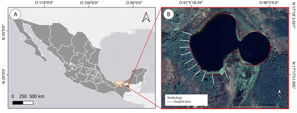
Figure 1. Location of the study area. A) Mexico, highlighting the state of Tabasco (orange) and the municipality of Tenosique (blue). B) El Cacahuate Lagoon (red outline) showing sampling transects (white lines) established in the mangrove vegetation.
The identification of the species was carried out with the support of taxonomic keys and specialized literature for the families Bromeliaceae, Cactaceae, and Orchidaceae (Alderete-Chávez & Capello-García, 1988; Ames & Correll, 1985; Beutelspacher, 2011; Campos-Díaz et al., 2020; Conap, 2010; Davidse et al., 1994; Espejo-Serna et al., 2004; Hágsater et al., 2005; Hietz & Hietz-Seifert, 1994; Martínez-Meléndez et al., 2011; Mondragón-Chaparro et al., 2011; Noguera-Savelli & Cetzal-Ix, 2014), as well as Aspleniaceae, Polypodiaceae, and Pteridaceae (Mickel & Smith, 2004). For species identification, original descriptions were reviewed in the Biodiversity Heritage Library (BHL, 2022). Additionally, to determine the conservation status of the recorded epiphyte species in the study area, we consulted the official Mexican environmental protection and species legislation NOM-059-Semarnat-2010 (Semarnat, 2010) and the Red List of Threatened Species by the International Union for Conservation of Nature (IUCN, 2021).
To determine similarities between the epiphyte species composition of the inland mangrove of El Cacahuate (IM-Cacahuate) and other epiphyte communities, available epiphyte floristic lists from various vegetation types were compiled within a 220 km radius starting from the study area, including sites in Mexico and Guatemala (Fig. 2). Radius length corresponds to the straight-lined distance between El Cacahuate Lagoon and the nearest coastal mangroves of Tabasco, Mexico. It is important to note that most of the studies reviewed were conducted with objectives and sampling efforts not specific to epiphytes, so only the epiphyte species reported were considered (excluding hemiepiphytes).
For the Mexican portion, the compiled lists correspond to coastal mangroves (CM-Paraíso: including localities of Cárdenas, Centla, Comalcalco, Paraíso, Tabasco; Díaz-Jiménez, 2007. CM-Centla: Centla, Tabasco; Jiménez-López et al., 2017, 2018. CM-Nohan: UMA Nohan, Cd. del Carmen, Campeche; Noguera-Savelli et al., 2021); high evergreen tropical forest (HETF-Tenosique: Tenosique, Tabasco, Hernández-Sastré et al., 2014); medium evergreen tropical forest (METF-Macuspana: Macuspana, Tabasco; López-Gómez, 2014; METF-Tenosique: Tenosique, Tabasco; Morales-Damián, 2012); medium subevergreen tropical forest (MSTF-Catazaja: Catazajá, Chiapas; Gutiérrez-Báez, 2004); and tropical dry forest (TDF-Tenosique: Tenosique, Tabasco; Morales-Damián, 2012). Additionally, the riparian flora list of the San Pedro Mártir River was included, which comprises epiphyte records in high, medium, and low evergreen tropical forests with the presence of R. mangle individuals in the riparian vegetation (TF&IM-San Pedro Mártir, Aburto-Oropeza et al., 2021). There are floristic lists that report the presence of epiphyte species for the Calakmul Biosphere Reserve, Campeche, (Conanp, 2023b; Martínez et al., 2001), which were not integrated into the database because this site belongs to the biotic province Yucatán Peninsula (Conanp, 2023b; García-Gil et al., 2002), which reports greater floristic affinity with the districts within the Yucatán Peninsula, Guatemala, and Belize (Duno-de Stefano et al., 2012) and the states of Chiapas, Oaxaca, and Veracruz (Ibarra-Manríquez et al., 2002; Morrone, 2019).
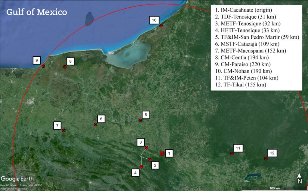
Figure 2. Location of El Cacahuate inland mangrove, the tropical forests, and coastal mangroves within a 220 km radius that include epiphytic floristic lists. The straight-line distance from each site to El Cacahuate is indicated in parentheses. Site acronyms are defined in the Materials and methods section.
In Guatemalan territory, only 2 floristic lists within the established distance for the analysis were obtained: one from a disturbed high evergreen tropical forest (TF-Tikal, Hellmuth & D’Angelo-Jerez, 2022), and the second from a high evergreen tropical forest combined with R. mangle from the El Petén area (TF&IM-Peten, Conap, 2010). Appendix presents the list of the recorded species in the present study and the species compiled from the reviewed studies. The classification of the types of vegetation is based on the proposal of Conabio (2013, 2019) for Chiapas and Tabasco, Mexico, and by Melgar (2003) and Conap (2010) for Tikal and El Petén, Guatemala.
A presence-absence data base was constructed, based on the epiphyte species recorded in our study area and the epiphyte species documented from the surrounding sites obtained of literature. The nomenclature was updated and standardized using the electronic database Tropicos (Tropicos, 2023). Subsequently, the similarity between epiphyte communities of the different vegetation types and locations was explored using the data matrix in a hierarchical clustering analysis (UPGMA) based on the Jaccard similarity index (JSI). This index was selected as it uses species presence-absence data, which was the type of data obtained from the reviewed studies. The measure of similarity ranges from 0% (not similar) to 100% (the most similar). Finally, a beta diversity analysis was performed using Cody’s index (Ci) to assess species turnover between communities. If a high index is obtained, it means that the sites are very different, while a low index means that they share most of their species. Both analyses were conducted using the program Past 4.12b (Hammer et al., 2001).
Results
A total of 6 families, 18 genera, and 27 species of epiphytes were recorded (Table 1)in El Cacahuate mangrove, with Orchidaceae and Bromeliaceae being the families with the highest number of species (11 and 10, respectively), followed by Cactaceae and Polypodiaceae (2 species each) and Aspleniaceae and Pteridaceae (1 species each; Fig. 3). The genera with the most species were Tillandsia (Bromeliaceae) with 8 species, and Epidendrum (Orchidaceae) with 3. Among the epiphyte species recorded in El Cacahuate, Asplenium serratum L. is listed as a threatened species under Mexican legislation (Semarnat, 2010), while Tillandsia fasciculata Sw. and Selenicereus grandiflorus (L.) Briton & Rose are cited on the Red List of Threatened Species by IUCN (2021) as species of least concern.
Table 1
List of epiphyte species associated with the mangrove of El Cacahuate Lagoon, Tenosique, Tabasco, Mexico. *New records for the Wanha’ Biosphere Reserve.
| Family | Species |
| Aspleniaceae | Asplenium serratum L.* |
| Bromeliaceae | Aechmea bracteata (Sw.) Griseb. |
| Catopsis morreniana Mez | |
| Tillandsia balbisiana Schult. & Schult.f. | |
| T. brachycaulos Schltdl. | |
| T. bulbosa Hook. | |
| T. dasyliriifolia Baker* | |
| T. fasciculata Sw. | |
| T. juncea (Ruiz & Pav.) Poir. | |
| T. schiedeana Steud. | |
| T. streptophylla Scheidw. Ex E.Morren | |
| Cactaceae | Deamia testudo (Karw. Ex Zucc.) Britton & Rose |
| Selenicereus grandiflorus (L.) Briton & Rose | |
| Orchidaceae | Catasetum integerrimum Hook. |
| Cohniella ascendens (Lindl.) Christenson | |
| Encyclia bractescens (Lindl.) Hoehne | |
| Epidendrum cardiophorum Schltr. | |
| E. diffusum Sw.* | |
| E. nocturnum Jacq. | |
| Myrmecophila tibicinis (Bateman) Rolfe | |
| Nidema boothi (Lindl.) Schltr.* | |
| Notylia barkerii Lindl.* | |
| Oncidium sphacelatum Lindl. | |
| Specklinia grobyi (Bateman ex Lindl.) F.Barros | |
| Polypodiaceae | Microgramma nítida (J. Sm.) A.R. Sm.* |
| Polypodium polypodioides (L.) Watt* | |
| Pteridaceae | Vittaria lineata (L.) Sm. |
Similarities between epiphyte communities. The present study and the review of published studies within the selected surrounding area allowed for the compilation of a total of 119 epiphyte species from sites with coastal mangrove, inland mangrove, tropical forests, and disturbed forests (Appendix). The sites with the highest number of epiphyte species were the high evergreen tropical forest of Tenosique (HETF-Teno, 53 species), the riparian vegetation of the San Pedro River (TF&IM-SPMR, 52 species), the medium evergreen tropical forest of Macuspana (METF-Macus, 45 species), the inland mangrove of El Cacahuate Lagoon (IM-Cac, 27 species), and the coastal mangrove of Centla (CM-Centla, 25 species). In the remaining sites, the number of epiphyte species ranged from 4 to 16, with 14 species recorded in the coastal mangroves of Nohan and Paraíso (CM-Nohan, CM-Paraíso; Appendix).
The clustering analysis (Fig. 4) clearly separated 4 groups (at a similarity level of 0.14). Two groups consisted of a single location: the first being the disturbed evergreen tropical forest of Tikal (TF-Tikal) and the second, the medium subevergreen tropical forest of Catazaja, Chiapas (MSTF-Catazaja). The other 2 groups contained several locations. The first group was made up of different forest types in Tabasco (HETF-Tenosique, METF-Macuspana, TDF-Tenosique, METF-Tenosique), while the second group included sites with coastal mangroves (CM-Nohan, CM-Paraíso, CM-Centla) and tropical forest and inland mangrove vegetation (TF&IM-San Pedro Mártir, TF&IM-Peten, IM-Cacahuate). In this latter group, the inland mangrove of El Cacahuate showed greater similarity in the epiphyte species with the coastal mangroves of Centla (JSI = 0.45, 16 shared species) and Paraíso (JSI = 0.38, 11 shared species), despite being 194 and 220 km away from El Cacahuate, respectively. The tropical forest and mangrove vegetation of the San Pedro River shared a greater number of species (19) with the El Cacahuate mangrove, but the similarity was slightly lower (JSI = 0.23), although the distance between these sites is lower, 59 km. The next ecosystem is the forest with inland mangrove of El Petén, sharing 8 species with El Cacahuate and showing a lower similarity than the previous groups (JSI = 0.18). At last, the coastal mangrove of Nohan, Campeche shared 7 species with El Cacahuate, with the lower similarity inner this group (JSI = 0.15).
Among all groups, the lowest similarity of the epiphyte community of El Cacahuate was with the medium subevergreen tropical forest of Catazaja (JSI = 0.05) and the disturbed evergreen tropical forest of Tikal (JSI = 0.03), with 2 and 1 species in common, respectively; both located over 100 km from El Cacahuate Lagoon. Among sites with mangrove vegetation, beta diversity analysis (Table 2) shows that the inland mangrove of El Cacahuate presents low species turnover with the coastal mangroves (Centla and Paraíso; Ci= 10 and 9.5, respectively). In contrast, species turnover is higher with the riparian forest and mangrove vegetation of the San Pedro Mártir River (Ci= 19).
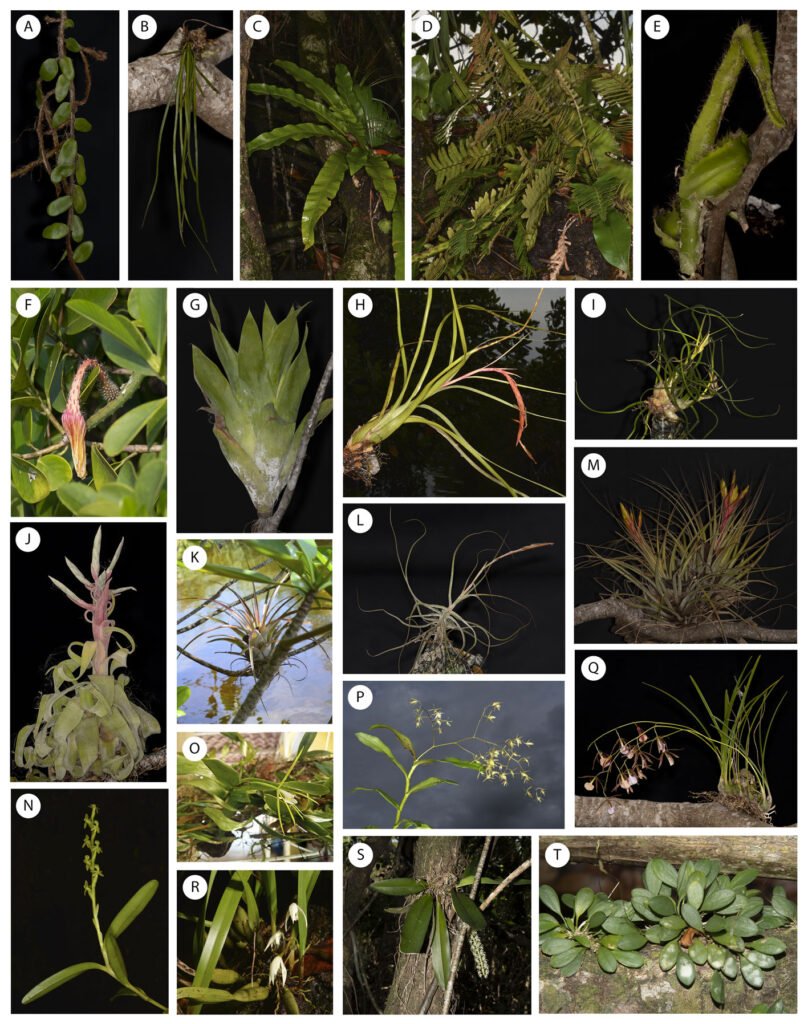
Figure 3. Representative epiphyte species recorded in the inland mangrove of El Cacahuate Lagoon, Tenosique, Tabasco, Mexico. A) Microgramma nitida, B) Vittaria lineata, C) Asplenium serratum, D) Polypodium polypodioides, E) Deamia testudo, F) Selenicereus grandiflorus, G) Catopsis morreniana, H) Tillandsia balbisiana, I) T. bulbosa, J) T. streptophylla, K) T. dasyliriifolia, L) T. schiedeana, M) T. fasciculata, N) Epidendrum cardiophorum, O) E. nocturnum, P) E. diffusum, Q) Encyclia bractescens, R) Nidema boothi, S) Notylia barkerii, and T) Specklinia grobyi. Photographs by Jesús Rodríguez and Neil Morales.
Discussion
As far as we know, our study is the first to be conducted on epiphytic species of inland mangroves in El Cacahuate Lagoon. The epiphyte community of El Cacahuate Lagoon, with 27 records species, is among the richest ever reported in a mangrove ecosystem. Previous studies have reported the presence of fewer species in coastal mangroves (De Sousa & Colpo, 2017; Díaz-Jiménez, 2007; Jiménez-López et al., 2017, 2018; Menéndez-Liguori, 1976; Noguera-Savelli et al., 2021; Rohani et al., 2020). However, it is true that many of these studies did not involve extensive sampling, or they were not specifically focused on epiphyte species. Jiménez-López et al. (2017, 2018), in the mangrove of El Cometa Lagoon, Centla, Tabasco, were specifically focused on epiphytes, recording 25 species. In contrast, the tropical forest sites of Tenosique and Macuspana (Hernández-Sastré et al., 2014; López-Gómez, 2014; Morales-Damián, 2012), and the riparian forest and mangrove of San Pedro Mártir, Tabasco (Aburto-Oropeza et al., 2021), have a higher reported number of epiphyte species than the mangrove of El Cacahuate. However, these differences in the number of species reported are because the forests of Tenosique, Macuspana, and the San Pedro Mártir River were collected in larger areas of vegetation, a greater number of phorophyte species were sampled, and different sampling methods were used. For example: A) in the forests of Tenosique (Morales-Damián, 2012; Hernández-Sastré et al., 2014) sampled 25 × 25 m plots, recording the epiphytes associated with 9 species of phorophytes; B) in the Macuspana forest (López-Gómez, 2014), a representative sampling method of 1 ha was used, sampling epiphytes in 8 plots of 20 × 20 m (400 m²), considering both trees and shrubs present; and finally C) on the San Pedro Mártir River (Aburto-Oropeza et al., 2021), targeted sampling was carried out between 2014 and 2015 with sporadic collections until 2019, covering more than 25 linear km of river and sampling more than 30 species of phorophytes (Burelo-Ramos pers. com.). This shows that floristic lists targeting forests tend to have higher reports of epiphytes than mangrove ecosystems.
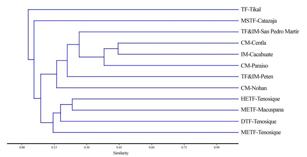
Figure 4. Dendrogram showing the similarity of epiphyte communities among the El Cacahuate Lagoon mangrove, coastal mangroves, and adjacent forest vegetation sites. Site acronyms are defined in the Materials and Methods section.
Table 2
Beta-diversity of epiphytes between the inland mangrove of El Cacahuate Lagoon and epiphyte floristic lists of surrounding tropical forest and coastal mangroves. Values above the diagonal represent Cody’s index for each pairwise comparison. Values below the diagonal indicate the number of shared species between sites. The top row displays the total species richness for each location. The first column lists the number of species unique to each site. Site acronyms are defined in the Materials and methods section.
| Total | 27 | 11 | 9 | 47 | 51 | 4 | 43 | 25 | 14 | 14 | 16 | 5 | |
| Unique | sites | IM-Cacahuate | TDF-Tenosique | METF-Tenosique | HETF-Tenosique | TF&IM-San Pedro | MSTF-Catazaja | METF-Macuspana | CM-Centla | CM-Paraíso | CM-Nohan | TF&IM-Peten | TF-Tikal |
| 0 | IM-Cacahuate | 12 | 15 | 23 | 19 | 13.5 | 29 | 10 | 9.5 | 13.5 | 13.5 | 15 | |
| 0 | TDF-Tenosique | 7 | 8 | 19 | 25 | 6.5 | 20 | 15 | 10.5 | 11.5 | 13.5 | 8 | |
| 0 | METF-Tenosique | 3 | 2 | 19 | 27 | 6.5 | 20 | 16 | 9.5 | 10.5 | 12.5 | 7 | |
| 11 | HETF-Tenosique | 14 | 10 | 9 | 32 | 24.5 | 28 | 29 | 24.5 | 26.5 | 28.5 | 24 | |
| 14 | TF&IM-SPMR | 20 | 6 | 3 | 17 | 24.5 | 32 | 23 | 21.5 | 26.5 | 24.5 | 25 | |
| 1 | MSTF-Catazaja | 2 | 1 | 0 | 1 | 3 | 21.5 | 11.5 | 8 | 7 | 10 | 4.5 | |
| 15 | METF-Macuspana | 5 | 6 | 6 | 17 | 15 | 2 | 28 | 26.5 | 26.5 | 29.5 | 24 | |
| 3 | CM-Cent | 16 | 3 | 1 | 7 | 15 | 3 | 6 | 8.5 | 11.5 | 13.5 | 14 | |
| 1 | CM-Para | 11 | 2 | 2 | 6 | 11 | 1 | 2 | 11 | 10 | 9 | 8.5 | |
| 5 | CM-Nohan | 7 | 1 | 1 | 4 | 6 | 2 | 2 | 7 | 4 | 13 | 9.5 | |
| 4 | TF&IM-Peten | 8 | 0 | 0 | 3 | 9 | 0 | 0 | 7 | 6 | 2 | 8.5 | |
| 1 | TF-Tikal | 1 | 0 | 0 | 2 | 3 | 0 | 0 | 1 | 1 | 0 | 2 |
The low richness of epiphytes in coastal mangroves has been associated with the adverse environmental conditions present, such as high temperatures, low precipitation, and excess salinity (Benzing, 1990; Carmona-Díaz et al., 2014; García-Luna et al., 2024; Gómez & Winker, 1991; Zimmerman & Olmsted, 1992; Zotz & Reuter, 2009). Mangrove trees eliminate excess salt through their leaves (Mikolaev et al., 2016; Zotz & Reuter, 2009), so large amounts of salt could be accumulating in some epiphytes (e.g., orchids and bromeliads) due to leaf litter and rainwater falling from the canopy, which is captured in the roots and the rosette leaves of these plants. Salt decreases the osmotic potential of epiphyte cells, reducing their survival by promoting tissue necrosis and leaf loss, especially for species that do not have adaptations to survive under extreme water stress conditions, v.gr., xerophytic habits (Benzing, 2000; Du & Hesp, 2020; Zotz & Reuter, 2009). However, Gómez and Winkler (1991) have pointed out a contrary position suggesting that the high precipitation in some coastal areas may dilute the high salinity that falls from the mangrove’s canopy, allowing for the existence of non-xerophytic epiphytes. Nevertheless, the low presence of epiphyte species in mangrove ecosystems suggests that the physiological limitations in many of these plants may be significant (Cach-Pérez et al., 2018). Considering the distribution of mangroves worldwide, more floristic studies are needed in this ecosystem to identify patterns in other epiphytes species numbers, physiological traits, and functional groups.
The mangrove of El Cacahuate Lagoon presents a less stressful environment compared to coastal mangroves, as it is in a freshwater body with high precipitation (annual average of 2,300 mm) and warm temperatures (annual average of 26 °C) (Aceves-Navarro & Rivera-Hernández, 2019). In coastal mangroves, which are characterized as saline ecosystems (Feller et al., 2010), R. mangle eliminates the excess of salt absorbed by its roots through lenticels on its leaves (Bento et al., 2024). However, although El Cacahuate Lagoon is a freshwater aquatic system (0.4 psu) compared to nearby coastal sites (22 psu), calcium carbonate from mountain runoff has been reported in the area (Aburto-Oropeza et al., 2021; Conanp, 2023a) and the sap salinity of the plants is like that of trees in coastal areas (J. López-Portillo pers. com.). This suggests that the R. mangle trees in El Cacahuate Lagoon still exude salt through the leaves. However, atmospheric humidity and high precipitation could dilute the concentration of salts reaching the epiphytes (J. López-Portillo pers. com.). These conditions seem to favor the presence of orchid, bromeliad, and fern species recorded at this site; it also suggests that the species shared between the inland mangrove and coastal mangroves have adapted to both environmental conditions. Specific ecophysiological studies of the shared and not shared epiphyte species between this inland mangrove and the coastal mangroves will provide a better understanding of the characteristics that limit and promote the distribution of epiphytes in these ecosystems.
Similarities between epiphyte communities. Given the proximity of the Tenosique mountain (ca. 2-32 km), we expected that the species composition of the study area showed greater similarity in epiphyte composition with the surrounding forests (HETF, METF, DTF). It has been recorded that the structure, anatomy, and seed dispersal mechanisms of many epiphytes permit frequent colonization and recolonization processes between nearby tropical sites (Chilpa-Galván et al., 2018; Toledo-Aceves et al., 2012). Nevertheless, we found the highest similarity of El Cacahuate mangrove’s epiphyte species with the epiphyte communities of the coastal mangroves of Centla and Paraíso, located 194-200 km away. These facts suggest 2 possible hypotheses which can help to explain these similarities: the first suggests that when the sea encroached 120,000 years ago, not only R. mangle individuals and other terrestrial coastal species established along the banks of the San Pedro River and El Cacahuate Lagoon, but this process was accompanied by the coastal-affinity epiphytes recorded in the study area; the second one points to contemporary dispersal processes as the reason for the presence of these epiphytes with a coastal distribution. It has been documented that after ca. 30 years, 30% of the original epiphyte species recorded in mangrove trees in the natural part of a canal, colonized juvenile mangroves planted for reforestation in the artificial part of the canal (Kupec, 2018). This suggests that the epiphyte species with coastal affinity may have arrived at the inland mangrove of El Cacahuate Lagoon by seed step-dispersal and colonization events throughout the mangrove established along the San Pedro River, or by long-distance dispersal events of minute seed from the coastal mangroves (Schurr et al., 2009). The other epiphyte species with extensive tropical forest distribution surely have arrived by both dispersal ways.
These 2 processes do not exclude each other, and their success can be highly dependent on the number of viables seeds and habitat availability (Rodríguez-Romero et al., 2011). However, successful establishment also depends on the morphological and anatomical characteristics of the seeds (Arditti & Ghani, 2000; Chilpa-Galván et al., 2018). For instance, some ferns families (e.g., Aspleniaceae, Polypodiaceae, and Pteridaceae) produce many very small spores that are easily dispersed by wind over long distances (Martínez-Salas & Ramos, 2014; Perrie et al., 2010; Shepherd et al., 2009). Similarly, orchid fruits (Orchidaceae) produce millions of tiny seeds, often just a few microns in size and weighing no more than 22 mcg (Arditti & Ghani, 2000; Menchaca-García & Moreno-Martínez, 2011), which are also adapted for long-distance wind dispersal. Many bromeliad species (Bromeliaceae, subfamily Tillandsoideae) have plumose seed appendages that facilitate their movement through the air and their attachment to rough bark surfaces (Einzmann & Zotz, 2017; Mondragón-Chaparro et al., 2011). Meanwhile, some species such as A. bracteata, which produce berry-like fruits, and cacti such as S. grandiflorus and D. testudo, which have pulpy fruits, are dispersed by birds. This suggests that short- or long-distance seed dispersal has contributed to structuring the epiphyte community in the inland mangrove of El Cacahuate Lagoon. Future genetic studies will reveal how closely related the populations of shared epiphyte species are between the inland mangroves of El Cacahuate Lagoon and the coastal mangroves of Tabasco, particularly for those species with a wide distribution range.
Our study clearly shows that the epiphyte community in the inland mangroves of El Cacahuate Lagoon is species-rich. The humid environmental conditions present apparently reduce the salinity concentration exuded by the mangrove trees, allowing the great epiphyte species richness recorded. Also, we have demonstrated that this epiphyte community has a high similarity in composition to the epiphyte communities of the coastal mangroves of Tabasco, suggesting a close genetic relationship between these populations. Future genetic studies will help elucidate the dispersal routes followed by the epiphytes to colonize this mangrove. These and other biological characteristics make this inland mangrove ecosystem one of great biodiversity and conservation value.
Acknowledgments
Special thanks to the UJAT herbarium for access to its facilities and the support provided during the cabinet phase. We are grateful to M. Ferrer, J. Rodríguez, and E. López for their help with the fieldwork. Special thanks to W. Miss and his family for their hospitality and for facilitating access to the study site. Thanks to S. Morales, C. Rodríguez, and I. Morales for providing transportation to the study site. We extend our gratitude to F. Jiménez H. and R. Adams for reviewing early drafts of this manuscript. This study is part of the requirements for obtaining a master’s degree for NEM. The work was supported by the Universidad Juárez Autónoma de Tabasco through the project “Biodiversity and conservation of the inland mangroves of the San Pedro Mártir River as elements for sustainable development in Balancán and Tenosique, Tabasco, Mexico” (No. 20220327), and the Centro para la Biodiversidad Marina y la Conservación, A.C. and Mares Mexicanos. The Consejo Nacional de Humanidades, Ciencia y Tecnología (Conahcyt) granted a scholarship to the first author for his master’s program.
Appendix. Checklist of vascular epiphytes recorded in the inland mangrove of El Cacahuate Lagoon, and compiled data from the floristic studies completed in a radius of 220 km from El Cacahuate Lagoon. Acronyms: IM-Cacahuate, inland mangrove of El Cacahuate, Tenosique, Tabasco; CM-Paraíso, coastal mangrove of Cárdenas, Centla, Comalcalco, Paraíso, Tabasco (Díaz-Jiménez, 2007); CM-Centla, coastal mangrove of Centla, Tabasco (Jiménez-López et al., 2017, 2018); CM-Nohan, coastal mangrove of the UMA Nohan, Cd. del Carmen, Campeche (Noguera-Savelli et al., 2021); HETF-Tenosique, high evergreen tropical forest of Tenosique, Tabasco (Hernández-Sastré et al., 2014); METF-Tenosique, medium evergreen tropical forest of Tenosique, Tabasco (Morales-Damián, 2012); METF-Macuspana: Macuspana, Tabasco; López-Gómez 2014); MSTF-Catazaja: medium subevergreen tropical forest of Catazajá, Chiapas (Gutiérrez-Báez, 2004); TDF-Tenosique: tropical dry forest of Tenosique, Tabasco (Morales-Damián, 2012); TF&IM-San Pedro Mártir: tropical forests with the presence of R. mangle individuals in the riparian vegetation of the San Pedro Mártir River (Aburto-Oropeza et al., 2021); TF-Tikal: disturbed high evergreen tropical forest (Hellmuth and D’Angelo-Jerez, 2022); TF&IM-Peten: high evergreen tropical forest combined with R. mangle from the El Petén area (Conap, 2010).
| Families | Species /sites | IM-Cacahuate | TDF-Tenosique | METF-Tenosique | HETF-Tenosique | TF&IM-San Pedro Mártir | MSTF-Catazaja | METF-Macuspana | CM-Centla | CM-Paraíso | CM-Nohan | TF&IM-Petén | TF-Tikal |
| Aspleniaceae | Asplenium auritum Sw. | x | |||||||||||
| Asplenium serratum L. | x | x | |||||||||||
| Bromeliaceae | Aechmea bracteata (Sw.) Griseb. | x | x | x | x | x | x | ||||||
| Aechmea mexicana Baker | x | ||||||||||||
| Aechmea tillandsoides (Mart. ex Schult. & Schult.f.) Baker | x | ||||||||||||
| Billbergia viridiflora H.Wendl. | x | ||||||||||||
| Catopsis morreniana Mez | x | x | |||||||||||
| Catopsis nutans (Sw.) Griseb. | x | ||||||||||||
| Tillandsia anceps G. Lodd. | x | ||||||||||||
| Tillandsia balbisiana Schult. & Schult.f. | x | x | x | x | x | x | |||||||
| Tillandsia brachycaulos Schltdl. | x | x | x | x | x | ||||||||
| Tillandsia bulbosa Hook. | x | x | x | x | x | ||||||||
| Tillandsia chlorophylla L. B. Smith | x | ||||||||||||
| Tillandsia dasyliriifolia Baker | x | x | x | x | |||||||||
| Tillandsia fasciculata Sw. | x | x | x | x | |||||||||
| Tillandsia festucoides Brongn. Ex Mez | x | x | |||||||||||
| Tillandsia filifolia Schldtl. & Cham. | x | x | |||||||||||
| Tillandsia ionantha Planch | x | ||||||||||||
| Tillandsia juncea (Ruiz & Pav.) Poir. | x | x | x | x | |||||||||
| Tillandsia recurvata (L.) L. | x | ||||||||||||
| Tillandsia polystachia (L.) L. | x | ||||||||||||
| Tillandsia pseudobaileyi C.S. Gardner | x | ||||||||||||
| Tillandsia pruinosa Sw. | x | ||||||||||||
| Tillandsia schiedeana Steud. | x | x | x | x | x | ||||||||
| Tillandsia streptophylla Scheidw. Ex E.Morren | x | x | x | x | x | x | |||||||
| Tillandsia usneoides (L.) L. | x | x | x | x | x | ||||||||
| Tillandsia valenzuelana A. Rich | x | ||||||||||||
| Cactaceae | Deamia testudo (Karw. Ex Zucc.) Britton & Rose | x | x | x | x | x | x | ||||||
| Pseudorhipsalis ramulosa (Salm-Dyck) Barthlott | x | ||||||||||||
| Epiphyllum crenatum (Lindl.) G.Don | x | ||||||||||||
| Epiphyllum hookeri Haw. | x | x | |||||||||||
| Epiphyllum phyllanthus (L.) Haw. | x | x | x | ||||||||||
| Rhipsalis baccifera (J.S. Muell.) Stearn | x | x | |||||||||||
| Selenicereus donkelaarii (Salm-Dick) Britton & Rose | x | ||||||||||||
| Selenicereus grandiflorus (L.) Briton & Rose | x | x | x | x | |||||||||
| Selenicereus undatus (Haw.) D.R. Hunt | x | ||||||||||||
| Gesneriaceae | Columnea schiedeana Schltdl. | x | |||||||||||
| Orchidaceae | Acianthera hondurensis (Ames) Pridgeon & M. W. Chase | x | x | ||||||||||
| Brassavola nodosa (L.) Lindl. | x | x | |||||||||||
| Brassia caudata (L.) Lindl. | x | x | |||||||||||
| Brassia maculata R. Br. | x | x | |||||||||||
| Camaridium pulchrum Schltr. | x | x | |||||||||||
| Campylocentrum micranthum (Lindl.) Maury | x | x | |||||||||||
| Catasetum integerrimum Hook. | x | x | x | x | x | x | x | x | |||||
| Chysis bractescens Lindl. | x | x | x | ||||||||||
| Coelia triptera (Sm.) G. Don ex Steud. | x | x | x | ||||||||||
| Cohniella ascendens (Lindl.) Christenson | x | x | x | x | x | x | x | ||||||
| Cohniella cosymbephorum (C. Morren) R. Jiménez & Carnevali | x | ||||||||||||
| Cohniella lindenii (Brongn.) M.W.Chase & N.H.Williams | x | x | |||||||||||
| Cohniella luridum (Lindl.) M.W. Chase & N.H. Williams | x | x | x | ||||||||||
| Cohniella Yucatánensis Cetzal & Carnevali | x | ||||||||||||
| Coryanthes picturata Rchb.f. | x | x | |||||||||||
| Cycnoches ventricosum Bateman | x | ||||||||||||
| Dichaea muricatoides Hamer & Garay | x | ||||||||||||
| Dichaea panamensis Lindl. | x | ||||||||||||
| Encyclia alata (Bateman) Schltr. | x | x | x | ||||||||||
| Encyclia bractescens (Lindl.) Hoehne | x | x | x | x | |||||||||
| Encyclia guatemalensis (Klotzsh) Dressler & G.E. Pollard | x | ||||||||||||
| Epidendrum anceps Jacq. | x | ||||||||||||
| Epidendrum cardiophorum Schltr. | x | x | x | ||||||||||
| Epidendrum difforme Jacq. | x | x | |||||||||||
| Epidendrum diffusum Sw. | x | x | x | ||||||||||
| Epidendrum flexuosum G. Mey. | x | x | |||||||||||
| Epidendrum nocturnum Jacq. | x | x | x | x | x | ||||||||
| Epidendrum stamfordianum Bateman | x | x | x | ||||||||||
| Gongora leucochila Lem. | x | x | |||||||||||
| Gongora unicolor Rolfe | x | ||||||||||||
| Isochilus carnosiflorus Lindl. | x | x | x | ||||||||||
| Lophiaris lindenii (Brongn.) Braem | x | x | |||||||||||
| Lophiaris oerstedii (Rchb. f.) R. Jiménez Carnevali & Dressler | x | x | x | x | x | ||||||||
| Lophiaris teaboana R. Jiménez, Carnevali & Tapia Muñoz | x | ||||||||||||
| Lycaste aromatica (Graham) Lindl. | x | ||||||||||||
| Maxillaria aciantha Rchb. f. | x | ||||||||||||
| Maxillaria crassifolia (Lindl.) Rchb. f. | x | x | x | x | |||||||||
| Maxillaria elatior (Rchb. f.) Rchb. f. | x | x | |||||||||||
| Maxillaria hedwigiae Hamer & Dodson | x | ||||||||||||
| Maxillaria tenuifolia Lindl. | x | x | |||||||||||
| Maxillaria uncata Lind. | x | ||||||||||||
| Maxillaria variabilis Bateman ex Lindl. | x | x | |||||||||||
| Myrmecophila christinae var. christinae Carnevali & Gómez-Juárez | x | ||||||||||||
| Myrmecophila tibicinis (Bateman) Rolfe | x | x | x | x | x | x | |||||||
| Nemaconia striata (Lindl.) Van den Berg, Salazar & Soto Arenas | x | x | |||||||||||
| Nidema boothi (Lindl.) Schltr. | x | x | x | x | x | x | |||||||
| Notylia barkeri Lindl. | x | x | x | x | x | x | |||||||
| Notylia orbicularis A.Rich. | x | ||||||||||||
| Oncidium sphacelatum Lindl. | x | x | x | x | x | ||||||||
| Ornithocephalus inflexus Lindl. | x | x | |||||||||||
| Platystele minimiflora (Schltr.) Garay | x | ||||||||||||
| Platythelys querceticola (Lindl.) Garay | x | ||||||||||||
| Platystele stenostachya (Rchb.f.) Garay | x | ||||||||||||
| Polystachya caracasana Rchb.f. | x | ||||||||||||
| Prosthechea cochleata (L.) W.E.Higgins | x | x | x | ||||||||||
| Prosthechea boothiana (Lindl.) W.E.Higgins | x | ||||||||||||
| Prosthechea livida (Lindl.) W.E.Higgins | x | ||||||||||||
| Prosthechea pygmaea (Hook.) W. E. Higgins | x | ||||||||||||
| Prosthechea radiata (Lindl.) W. E. Higgins | x | ||||||||||||
| Restrepiella ophiocephala (Lindl.) Garay & Dunst. | x | ||||||||||||
| Sarcinula brighamii (S. Watson) Luer | x | ||||||||||||
| Scaphyglottis confusa (Schltr.) Ames & Correll | x | x | |||||||||||
| Specklinia grobyi (Bateman ex Lindl.) F.Barros | x | x | |||||||||||
| Specklinia picta (Lindl.) Pridgeon & M.W. Chase | x | ||||||||||||
| Specklinia pisinna (Luer) Solano y Soto Arenas | x | ||||||||||||
| Stelis gracilis Ames | x | ||||||||||||
| Tribulago tribuloides (Sw.) Luer | x | ||||||||||||
| Trichosalpinx ciliaris (Lindl.) Luer | x | ||||||||||||
| Trigonidium egertonianum Bateman ex Lindl. | x | x | x | x | |||||||||
| Piperaceae | Peperomia angustata Kunth | x | |||||||||||
| Peperomia cobana C.DC. | x | ||||||||||||
| Peperomia glutinosa Millsp. | x | ||||||||||||
| Peperomia obtusifolia (L.) A.Dietr. | x | ||||||||||||
| Peperomia quadrifolia (L.) Kunth | x | ||||||||||||
| Peperomia rotundifolia (L.) Kunth | x | ||||||||||||
| Polypodiaceae | Campyloneurum angustifolium (Sw.) Fée | x | |||||||||||
| Neurodium lanceolatum (L.) Fée | x | ||||||||||||
| Microgramma nitida (J. Sm.) A.R. Sm. | x | x | |||||||||||
| Phlebodium decumanum (Willd.) J. Sm. | x | ||||||||||||
| Polypodium polypodioides (L.) Watt | x | x | x | ||||||||||
| Pteridaceae | Antrophyum ensiforme Hook. | x | |||||||||||
| Vittaria lineata (L.) Sm. | x | x | x |
References
Aburto-Oropeza, O., Burelo-Ramos, C. M., Ezcurra, E., Ezcurra, P., Henriquez, C. L., Vanderplank, S. et al. (2021). Relict inland mangrove ecosystem reveals Last Interglacial sea levels. Proceedings of the National Academy of Sciences, 118, 1–8. https://doi.org/10.1073/pnas.2024518118
Aceves-Navarro, L. A., & Rivera-Hernández, B. (2019). Clima. In A. Cruz Angón (Ed.), La biodiversidad del estado de Tabasco. Estudio de estado (pp. 123–132). México, D.F.: Comisión Nacional para el Conocimiento y Uso de la Biodiversidad.
Aksornkoae, S. (1993). Ecology and management of mangroves. Bangkok, Thailand: International Union for Conservation of Nature (IUCN). https://portals.iucn.org/library/sites/library/files/documents/WTL-024.pdf
Alderete-Chávez, A., & Capello-García, S. (1988). Orquídeas de Tabasco. Villahermosa: Instituto Nacional de Investigaciones sobre Recursos Bióticos/ Instituto de Cultura de Tabasco.
Ames, O., & Correll, D. S. (1985). Orchids of Guatemala and Belize. New York: Dover Publications.
Arditti, J., & Ghani, A. K. A. (2000). Numerical and physical properties of orchid seeds and their biological implications. New Phytologist, 145, 367–421. https://doi.org/10.1046/j.1469-8137.2000.00587.x
Bento, J. P. S. P., Victório, C. P., Plaça, L. F., Arruda, R. C. O. (2024). Salt extrusion, a new function of lenticels in red mangrove leaves. Environmental and Experimental Botany, 223, 05798. https://doi.org/10.1016/j.envexpbot.2024.105798
Benzing, D. H. (1990). Vascular epiphytes: general biology and related biota. Cambridge, UK: Cambridge University Press.
Benzing, D. H. (2000). Bromeliaceae: profile of an adaptative radiation. Cambridge, UK: Cambridge University Press.
Beutelspacher, C. R. (2011). Guía de orquídeas de Chiapas. Tuxtla Gutiérrez, Chiapas: Universidad de Ciencias y Artes de Chiapas. Chiapas
BHL (Biodiversity Heritage Library) (2022). Available at: https://www.biodiversitylibrary.org
Cach-Pérez, M. J., Andrade, J. L., Chilpa-Galván, N., Tamayo-Chim, M., Orellana, R., & Reyes-García, C. (2013). Climatic and structural factors influencing epiphytic bromeliad community assemblage along a gradient of water-limited environments in the Yucatán Peninsula, Mexico. Tropical Conservation Science, 6, 283–302. https://doi.org/10.1177/194008291300600209
Campos-Díaz, M. J., Burelo-Ramos, C. M., & Arias, S. (2020). La familia Cactaceae en Tabasco, México. Acta Botanica Mexicana, 127, e1635. https://doi.org/10.21829/abm127.2020.1635
Carmona-Díaz, G., Hernández-Carmona, S., Morales-Mávil, J. E., Hernández-Salazar, L. T., & García-Orduña, F. (2014). Contribución al conocimiento ecológico de la epífita vascular Aechmea bracteata (Bromeliaceae) en el manglar de Sontecomapan, Catemaco, Veracruz, México. Revista Científica Biológico Agropecuario, Tuxpan, 2, 816–821.
Carmona-Higuita, M. J., Mendieta-Leiva, G., Gómez-Díaz, J. A., Villalobos, F., Ramos, F. N., Elias, J. P. C. et al. (2025). Endemism centres of the five richest vascular epiphyte families in the Neotropics. Journal of Biogeography, 52, 80–91. https://doi.org/10.1111/jbi.15016
Ceja-Romero, J., Espejo-Serna, A., López-Ferrari, A. R., García-Cruz, J., Mendoza-Ruiz, A., & Pérez-García, B. (2008). Las plantas epífitas, su diversidad e importancia. Ciencias, 1, 34–41.
Chilpa-Galván, N., Márquez-Guzmán, J., Zotz, G., Echevarría-Machado, I., Andrade, J. L., Espadas-Manrique, C. et al. (2018). Seed traits favouring dispersal and establishment of six epiphytic Tillandsia (Bromeliaceae) species. Seed Science Research, 28, 349–359. https://doi.org/10.1017/S0960258518000247
Conabio (Comisión Nacional para el Conocimiento y Uso de la Biodiversidad) (2013). La biodiversidad en Chiapas: Estudio de Estado. México: Conabio/ Gobierno del Estado de Chiapas.
Conabio (Comisión Nacional para el Conocimiento y Uso de la Biodiversidad) (2019). La biodiversidad en Tabasco. Estudio de Estado. México: Conabio. https://bioteca.biodiversidad.gob.mx/janium/Documentos/14868.pdf
Conap (Consejo Nacional de Áreas Protegidas) (2010). Guía de reconocimiento del género Tillandsiade Guatemala. Guatemala. https://www.caftadr-environment.org/wp-cont
ent/uploads/2016/04/guia-de-Reconocimiento-de-Tillandsia-2.pdf
Conanp (Comisión Nacional de Áreas Naturales Protegidas) (2015). Área de protección de flora y fauna Cañon del Usumacinta. México: Semarnat/ Conanp. https://www.
conanp.gob.mx/que_hacemos/pdf/programas_manejo/2015/Canon_del_Usumacinta.pdf
Conanp (Comisión Nacional de Áreas Naturales Protegidas) (2023a). Estudio previo justificativo para el establecimiento del Área Natural Protegida Reserva de la Biósfera Wanha’.Tabasco, México. https://www.conanp.gob.mx/pdf/separata/EPJ-RB-Wanha.pdf
Conanp (Comisión Nacional de Áreas Naturales Protegidas) (2023b). Estudio previo justificativo para la modificación de la declaratoria del Área Natural Protegida Reserva de la Biosfera Calakmul, Campeche, México. https://www.conanp.gob.mx/pdf/separata/EPJ-Modificacion-RB-Calakmul.pdf
Davidse, G., Sousa-Sánchez, M., & Chater, A. O. (1994). Alismataceae a Cyperaceae. In G. Davidse (Ed.), Flora mesoamericana (pp. 1–543). México D.F.: Universidad Nacional Autónoma de México.
De Sousa, M. M., & Colpo, K. D. (2017). Diversity and distribution of epiphytic bromeliads in a Brazilian subtropical mangrove. Anais da Academia Brasileira de Ciências, 89, 1085–1093. https://doi.org/10.1590/0001-3765201720160702
Díaz-Jiménez, P. (2007). Flora epífita de los manglares de Tabasco, México. Kuxulkab, 13, 11–17.
Du, J., & Hesp, P. A. (2020). Salt spray distribution and its impact on vegetation zonation on coastal dunes: a review. Estuaries and Coasts, 43, 1885–1907. https://doi.org/10.1007/s12237-020-00820-2
Duno-de Stefano, R., Can-Itza, L. L., Rivera-Ruiz, A., & Calvo-Irabién, L. M. (2012). Regionalización y relaciones biogeográficas de la península de Yucatán con base en los patrones de distribución de la familia Leguminosae. Revista Mexicana de Biodiversidad, 83, 1053–1072. https://doi.org/10.7550/rmb.27824
Einzmann, H. J., & Zotz, G. (2017). Dispersal and establishment of vascular epiphytes in human-modified landscapes. AoB Plants, 9. https://doi.org/10.1093/aobpla/plx052
Espejo-Serna, A., López-Ferrari, A. R., Ramírez-Morillo, I., Holst, B., Luther, H., & Till, W. (2004). Checklist of Mexican Bromeliaceae with notes on species distribution and levels of endemism. Selbyana, 25, 33–86. https://doi.org/10.2307/41760147
Feller, I. C., Lovelock, C. E., Berger, U., McKee, K. L., Joye, S. B., & Ball, M. C. (2010). Biocomplexity in Mangrove Ecosystems. Annual Review of Marine Science, 2, 395–417. https://doi.org/10.1146/annurev.marine.010908.163809
Flores-Palacios, A., & García-Franco, J. G. (2006). The relationship between tree size and epiphyte richness: testing four different hypotheses. Journal of Biogeography, 33, 323–330. https://doi.org/10.1111/j.1365-2699.2005.01382.x
García-Gil, G., Palacio-Prieto, J. L., & Ortiz-Pérez, M. A. (2002). Reconocimiento geomorfológico e hidrográfico de la Reserva de la Biosfera Calakmul, México. Investigaciones Geográficas, 48, 7–23. https://doi.org/10.14350/rig.59170
García-Luna, C., Carrillo-Bastos, A., Cutz-Pool, L. Q., & González-Salvatierra, C. (2024). Composición de las epífitas vasculares asociadas al manglar ribereño en la comunidad de Ramonal, Quintana Roo, México. Madera y Bosques, 30, e3042616. https://doi.org/10.21829/myb.2024.3042616
Gutiérrez-Baéz, C., & Zamora-Crescencio, P. (2022). Listado florístico de la zona arqueológica de Calakmul, Campeche, México. Foresta Veracruzana, 24, 1–6.
Gómez, M. A., & Winkler, S. (1991). Bromelias en manglares del Pacífico de Guatemala. Revista de Biología Tropical, 39, 207–214.
Granados-Sánchez, D., López-Ríos, G. F., Hernández-García, M. Á., & Sánchez-González, A. (2003). Ecología de las plantas epífitas. Revista Chapingo. Serie Ciencias Forestales y del Ambiente, 9, 101–111.
Gutiérrez-Báez, C. (2004). Listado florístico del norte de Chiapas: Catazajá y límites con Palenque. Polibotánica, 17, 107–124.
Hágsater, E., Soto-Arenas, G. A., Salazar, G. A., Jiménez-Machorro, R., López-Rosas, M. A., & Dressler, R. L. (2005). Orchids of Mexico. México: Instituto Chinoin.
Hammer, O., Harper, D. A. T., & Ryan, P. D. (2001). PAST: Paleontological statistics software package for education and data analysis. Paleontología Electrónica, 4, 9.
Hellmuth, N., & D’Angelo-Jerez, S. (2022). Epífitas en una de las ceibas gigantes más populares de Tikal Plantas que crecen en las ramas y extremidades de los árboles. Guatemala: Flaar Mesoamérica. https://flaar-mesoamerica.org/wp-content/uploads/2023/01/PANAT-epiphytes-giant-Ceiba-Jul-20-2022-SJ-Sep-2022-espanol-PM-Nov-2022.pdf
Hernández-Sastré, J., Jiménez-Pérez, N. C., & Guadarrama-Olivera, M. A. (2014). Diversidad y estructura vertical de la comunidad de epífitas vasculares del Ejido Niños Héroes de Chapultepec, Tenosique, Tabasco (Bachelor´s Thesis). México. Universidad Juárez Autónoma de Tabasco.
Hietz, P., & Hietz-Seifert, U. (1994). Epífitas de Veracruz: guía ilustrada para las regiones de Xalapa y Los Tuxtlas. México: Instituto de Ecología A. C.
Hietz, P., & Hietz-Seifert, U. (1995). Composition and ecology of vascular epiphyte communities along an altitudinal gradient in central Veracruz, Mexico. Journal of Vegetation Science, 6, 487–498. https://doi.org/10.2307/3236347
Ibarra-Manríquez, G., Villaseñor, J. L., Durán, R., & Meave, J. (2002). Biogeographical analysis of the tree flora of the Yucatán Peninsula. Journal of Biogeography, 29, 17–29. https://doi.org/10.1046/j.1365-2699.2002.00648.x
IUCN (International Union for Conservation of Nature) (2021). The IUCN Red List of Threatened Species. Version 2021-3. Available at: https://www.iucnredlist.org.
Jiménez-López D. A., Roblero-Velasco R. de J., Martínez-Meléndez N., Ocampo G., & Gallardo-Cruz J.A. (2017). Relación entre variables del forófito y la riqueza de epífitas vasculares en los Pantanos de Centla, Tabasco, México. Acta Botanica Mexicana, 121, 125–137. https://doi.org/10.21829/abm121.2017.1179
Jiménez-López, D. A., Peralta-Carreta, C., Solórzano, J. V., Cervantes-Jiménez, G. L., & Domínguez-Vázquez, M. A. (2018). A checklist of vascular epiphytes of El Cometa Lagoon, Pantanos de Centla Biosphere Reserve, México. Journal of Threatened Taxa, 10, 12589–12597. https://doi.org/10.11609/jot.3794.10.11.12589-12597
Kelly, D. L., O’Donovan, G., Feehan, J., Murphy, S., Drangeid, S. O., & Marcano-Berti, L. (2004). The epiphyte communities of a montane rain forest in the Andes of Venezuela: patterns in the distribution of the flora. Journal of Tropical Ecology, 20, 643–666. https://doi.org/10.1017/S0266467404001671
Krömer, T., García-Franco, J. G., & Toledo-Aceves, T. (2014). Epífitas vasculares como bioindicadores de la calidad forestal: impacto antrópico sobre su diversidad y composición. In: C. A González Zuarth, A. Vallarino, JC Pérez Jiménez & AM Low (Eds.), Bioindicadores: guardianes de nuestro futuro ambiental (pp. 605–624). México: Ecosur/ Inecc.
Krömer, T., Gradstein, S. R., & Acebey, A. (2007). Diversidad y ecología de epífitas vasculares en bosques montanos primarios y secundarios de Bolivia. Ecología en Bolivia, 42, 23–33.
Krömer, T., & Gradstein, S. R. (2016). Vascular epiphytes. In T. H. Larsen (Ed.), Core standardized methods for rapid biological field assessment (pp. 25–36). USA: Conservation International.
Kupec, A. (2018). The comparison of vascular epiphytes diversity related to their occurrence in natural and artificial mangrove channels, Greenfields, eastern coast of Nicaragua. In S. Sharma (Ed.), Mangrove Ecosystem Ecology and Function (pp. 41–52). Malaysia: IntechOpen. https://doi.org/10.5772/intechopen.79133
Leal, M., & Spalding, M. D. (2021). The state of the World’s Mangroves 2021. Global Mangrove Alliance. https://www.mangrovealliance.org/wp-content/uploads/2022/09/The-State-of-the-Worlds-Mangroves-Report_2022.pdf
López-Gómez, D. (2014). Efecto de borde sobre la biodiversidad de orquídeas epifitas en el Parque Estatal de Agua Blanca, Macuspana, Tabasco, México (Bachelor’s Thesis). Universidad Juárez Autónoma de Tabasco. Tabasco, México.
Lot, A., & Chiang, F. (1986). Manual de Herbario, administración y manejo de colecciones, técnicas de recolección y preparación de ejemplares botánicos. México D.F.: Consejo Nacional de la Flora de México.
Lugo, A. E. (1981). The inland mangroves of Inagua. Journal of Natural History, 15, 845–852. https://doi.org/10.1080/00222938100770611
Martínez, E., Sousa, M., & Ramos-Álvarez, C. H. (2001). Listados florísticos de México XXII. Región de Calakmul, Campeche. México D.F.: Instituto de Biología, Universidad Nacional Autónoma de México.
Martínez-Meléndez, N., Martínez-Camilo, R., Pérez-Farrera, M. A., & Martínez-Meléndez, J. (2011). Las epífitas de la Reserva El Triunfo, Chiapas. Guía ilustrada de las especies más notables. Tuxtla Gutiérrez, Chiapas: UNICACH.
Martínez-Salas, E., & Ramos, C. H. (2014). Biodiversidad de Pteridophyta en México. Revista Mexicana de Biodiversidad, 85 (Suppl.), S110-S113. https://doi.org/10.7550/rmb.31827
Melgar, W. (2003). Estado de la diversidad biológica de los árboles y bosques de Guatemala. Documentos de Trabajo: Recursos Genéticos Forestales. Roma, Italia: Dirección de Recursos Forestales, FAO.
Menchaca-García, R. A., & Morano-Martínez, D. (2011). Manual para la propagación de orquídeas. Jalisco, México: Comisión Nacional Forestal/ Semarnat. http://www.conafor.gob.mx:8080/biblioteca/ver.aspx?articulo=462
Menéndez-Liguori, F. (1976). Los manglares de la laguna de Sontecomapan los Tuxltas, Veracruz: estudio florístico-ecológico (Bachelor’s Thesis). Universidad Nacional Autónoma de México. México.
Mickel J. T., & Smith A. R. (2004). The Pteridophytes of Mexico. New York: Botanical Garden Press.
Mikolaev, Y. O., Bernal, E. S., Baños, J. B., Escobar, M. O., & Hernández, J. G. (2016). Saline year-gradients in the lagoon “La Salina,” Tonameca, Oaxaca, Mexico: Effects on growth of mangrove biotope. Water, Air, & Soil Pollution, 227, 426. https://doi.org/10.1007/s11270-016-3133-3
Mondragón-Chaparro, D. M., Ramírez, I. M., Flores, M. M., & García, J. G. (2011). La Familia Bromeliaceae en México. Texcoco, Estado de México: Universidad Autónoma de Chapingo.
Morales-Damián, A. (2012). Inventario de orquídeas del ejido Niños Héroes de Chapultepec, Tenosique, Tabasco (Bachelor’s Thesis). Villahermosa: Universidad Juárez Autónoma de Tabasco.
Morrone, J. J. (2019). Regionalización biogeográfica y evolución biótica de México: encrucijada de la biodiversidad del Nuevo Mundo. Revista Mexicana de Biodiversidad, 90, e902980. https://doi.org/10.22201/ib.20078706e.2019.90.2980
Noguera-Savelli, E., Pacheco-Pizano, J., & Cetzal-Ix, W. (2021). Epífitas del fragmento de manglar de la UMA Nohan, Carmen, Campeche, México. Desde el Herbario CICY 13, 136–142.
Noguera-Savelli, E., & Cetzal-Ix, W. (2014). Revisión e integración del conocimiento de las Orchidaceae de Tabasco, México. Botanical Sciences, 92, 519–540. https://doi.org/10.17129/botsci.117
Palma-López, D. J., Jiménez Ramírez, R., Zavala-Cruz, J., Bautista-Zúñiga, F., Gavi-Reyes, F., & Palma-Cancino, D. Y. (2017). Actualización de la clasificación de suelos de Tabasco, México. Agroproductividad, 10, 29–35.
Patel, P. (2014). Inland mangroves of the world. Current Science, 107, 1094.
Patel, P., & Agoramoorthy, G. (2012). India’s rare inland mangroves deserve protection. Environmental Science & Technology, 46, 4261–4262. https://doi.org/10.1021/es301062v
Perrie, L. R., Ohlsen, D. J., Shepherd, L. D., Garrett, M., Brownsey, P. J., & Bayly, M. J. (2010). Tasmanian and Victorian populations of the fern Asplenium hookerianum result from independent dispersals from New Zealand. Australian Systematic Botany, 23, 387–392. https://doi.org/10.1071/SB10028
Rahman, M. S., Hossain, G. M., Khan, S. A., & Uddin, S. N. (2015). An annotated checklist of the vascular plants of Sundarban Mangrove Forest of Bangladesh. Bangladesh Journal Plant Taxon, 22, 17–41. https://doi.org/10.3329/bjpt.v22i1.23862
Rodríguez-Romero, M. L., Zavala-Hurtado, J. A., & Pacheco, L. (2011). Presencia, abundancia y estrategias reproductivas de helechos en áreas alteradas de la Sierra Nevada, México. Revista de Biología Tropical, 59, 417–433.
Rohani, S., Lee, F. L., & Yusoff, A. S. (2020). Diversity and vertical distribution of vascular epiphytes on a Malaysian mangrove island. Biotropia, 27, 134–142. https://doi.org/10.11598/btb.2020.27.2.1182
Rzedowski, J. (1996). Análisis preliminar de la flora vascular de los bosques mesófilos de montaña de México. Acta Botanica Mexicana, 35, 25–44. https://doi.org/10.21829/abm35.1996.955
Schurr, F. M., Spiegel, O., Steinitz, O., Trakhtenbrot, A., Tsoar, A., & Nathan, R. (2009). Long-distance seed dispersal. Annual Plant Reviews, 38, 204–237. https://doi.org/10.1002/9781444314557.ch6
Semarnat (Secretaría del Medio Ambiente y Recursos Naturales) (2010). Norma Oficial Mexicana NOM-059-Semarnat-2010, Protección ambiental – Especies nativas de México de flora y fauna silvestres – Categorías de riesgo y especificaciones para su inclusión, exclusión o cambio – Lista de especies en riesgo. Diario Oficial de la Federación. 2da Sección, 30 de diciembre de 2010.
Semarnat (Secretaría del Medio Ambiente y Recursos Naturales) (2023). Edicto: Reserva de la Biosfera la región denominada Wanha’, ubicada en los municipios de Balancán y Tenosique, en el estado de Tabasco, México. Diario Oficial de la Federación. 9 de agosto de 2023. https://dof.gob.mx/nota_detalle.php?codigo=5698495&fecha=15/08/2023#gsc.tab=0
Shepherd, L. D., De Lange, P. J., & Perrie, L. R. (2009). Multiple colonizations of a remote oceanic archipelago by one species: how common is long-distance dispersal? Journal of Biogeography, 36, 1972–1977. https://doi.org/10.1111/j.1365-2699.2009.02120.x
Sousa, M. M. D., & Colpo, K. D. (2017). Diversity and distri-
bution of epiphytic bromeliads in a Brazilian subtropical mangrove. Anais da Academia Brasileira de Ciências, 89, 1085–1093. https://doi.org/10.1590/0001-3765201720160702
Stoddart, D. R., Bryan, G. W., & Gibbs, P. E. (1973). Inland mangroves and water chemistry, Barbuda, West Indies. Journal of Natural History, 7, 33–46. https://doi.org/10.1080/00222937300770031
Taylor, F. J. (1986). Mangroves in freshwater. Blumea: Biodiversity, Evolution and Biogeography of Plants, 31, 271–272.
Thiers. B. (2021). Index Herbariorum: a global directory of public herbaria and associated staff. New York Botanical Garden’s Virtual Herbarium. Retrieved March 2024, from http://sweetgum.nybg.org/ih
Toledo-Aceves, T., García-Franco, J. G., Hernández-Rojas, A., & MacMillan, K. (2012). Recolonization of vascular epiphytes in a shaded coffee agroecosystem. Applied Vegetation Science, 15, 99–107. https://doi.org/10.1111/j.1654-109X.2011.01140.x
Tripathi, N., Singh, R. S., Bakhori, B., Dalal, C., Parmar, D. & Mishra, B. (2013). The World’s only inland mangrove in sacred grove of Kachchh, India, is at risk. Current Science, 105, 1053–1055.
Tropicos.org. (2023) Available at: https://tropicos.org
Woodroffe, C. D. (1988). Relict mangrove stand on last interglacial terrace, Christmas Island, Indian Ocean. Journal of Tropical Ecology, 4, 1–17. https://doi.org/10.1017/S0266467400002431
Zimmerman, J. K., & Olmsted, I. C. (1992). Host tree utilization by vascular epiphytes in a seasonally inundated forest (Tintal) in Mexico. Biotropica, 24, 402–407. https://doi.org/10.2307/2388610
Zotz, G. (2016). Physiological ecology. In G. Zotz (Ed.), Plants on plants: the biology of vascular epiphytes (pp. 95–137). Switzerland: Springer Cham. https://doi.org/10.1007/978-3-319-39237-0
Zotz, G., & Reuter, N. (2009). The effect of exposure to sea water on germination and vegetative growth of an
epiphytic bromeliad. Journal of Tropical Ecology, 25, 311–319. https://doi.org/10.1017/S0266467409006014
Zotz, G., Weigelt, P., Kessler, M., Kreft, H., & Taylor, A. (2021). EpiList 1.0: a global checklist of vascular
epiphytes. Ecology, 102, e03326. https://doi.org/10.1002/ecy.3326

Abundance and diversity of seeds dispersed by the Eastern cottontail (Sylvilagus floridanus) in an urban reserve in Mexico City
Abundancia y diversidad de semillas dispersadas por el conejo castellano (Sylvilagus floridanus) en una reserva urbana de la Ciudad de México
Yury Glebskiy a, b, *, Zenón Cano-Santana a
a Universidad Nacional Autónoma de México, Facultad de Ciencias, Departamento de Ecología y Recursos Naturales, Laboratorio de Interacciones y Procesos Ecológicos, Circuito Exterior s/n, Ciudad Universitaria, 04510 Ciudad de México, Mexico
b Universidad Nacional Autónoma de México, Posgrado en Ciencias Biológicas, Facultad de Ciencias, Circuito Exterior s/n, Ciudad Universitaria, 04510 Ciudad de México, Mexico
*Corresponding author: agloti@ciencias.unam.mx (Y. Glebskiy)
Received: 05 February 2025; accepted: 07 October 2025
Abstract
Lagomorphs are potentially important but understudied seed dispersers. In particular, there are no studies about the role of the Eastern Cottontail as a seed disperser. Therefore, the aim of this article is to evaluate the abundance and diversity of seeds dispersed by Sylvilagus floridanus in a conservation reserve within Mexico City. We collected fecal pellets during 2 periods, the highest seed production and the start of seed germination in the Reserva Ecológica del Pedregal de San Ángel. Pellets were subjected to different treatments to end seed dormancy (left in the field, stored in laboratory, and no treatment) and put to germinate in germination chambers and the field. We found that pellets left in the field had the most seeds germinating. Cottontails dispersed up to 0.77 seeds/g of excrete. A total of 15 species were observed, but the Chao estimator suggested that there were 29.8 species. Many of the dispersed seeds belong to rare species, most noticeable Jaegeria hirta. We conclude that cottontails are important dispersers due to the amount of excretes produced and the identity of the plants they disperse.
Keywords: Dormancy; Germination; Jaegeria hirta; Opuntia tomentosa;REPSA
Resumen
Los lagomorfos son dispersores de semillas potencialmente importantes, pero subestudiados. En particular, no existen estudios sobre el papel del conejo castellano como dispersor de semillas; por tanto, el objetivo de este artículo fue evaluar la abundancia y diversidad de semillas dispersadas por Sylvilagus floridanus en una reserva dentro de la Ciudad de México. Colectamos pastillas fecales durante 2 periodos, la temporada de mayor producción de semillas y el inicio de la germinación en la Reserva Ecológica del Pedregal de San Ángel. Las pastillas se sometieron a distintos tratamientos para terminar la dormancia (almacenar en el campo, en laboratorio y sin tratamiento) y fueron puestas a germinar en cámaras y en el campo. Encontramos que las excretas almacenadas en el campo tuvieron más semillas germinadas. Los conejos dispersaron hasta 0.77 semillas/g de excreta. Observamos 15 especies, pero el estimador de Chao sugirió que hubo 29.8 especies dispersadas. Muchas especies dispersadas son raras, en particular Jaegeria hirta. Concluimos que los conejos son importantes dispersores por la cantidad de excretas que producen y la identidad de las plantas diseminadas.
Palabras clave: Dormancia; Germinación; Jaegeria hirta; Opuntia tomentosa; REPSA
Introduction
There is a general consensus among ecologists that seed dispersal by animals is a very important service and that many plant species and even ecosystems could be dependent on this process (Gelmi-Candusso & Hämäläinen, 2019; Godó et al., 2022; Iluz, 2011). And there is an important amount of information on seed dispersal by birds, primates, and ungulates, among other groups (Albert et al., 2015; Beaune et al., 2013; Iluz, 2011); however, information on some other potentially important dispersers, particularly the lagomorphs, is scarce (Godó et al., 2022).
Lagomorphs are a widely distributed and abundant group of mammals that can be found across many ecosystems in all continents, except Antarctica (Chapman & Flux, 2008). Previous studies have shown that lagomorphs are not particularly important seed dispersers when compared to other animals by the number of seeds per gram of excrete (Borchert & Tyler, 2023; Malo & Suárez, 1995). However, they do disperse seeds, and given their abundance and the high amount of fecal matter they produce, they still have the potential to be important seed dispersers. Despite that, there are few studies that evaluate the role of lagomorphs as seed dispersers, and most of them used Oryctolagus cuniculus as the study model (Godó et al., 2022). Therefore, the aim of this study is to describe the diversity and abundance of seeds dispersed by endozoochory by the Eastern cottontail (Sylvilagus floridanus) in an urban reserve in Mexico City.
There are several studies about seed dispersal by the genus Sylvilagus, and they have found that species of this genus can be important seed dispersers of Opuntia (Borchert & Tyler, 2023) and Juniperus (Lezama-Delgado et al., 2016). At the same time, S. floridanus has a diverse diet (Chapman et al., 1980; Hudson et al., 2005). Therefore, our prediction was that Opuntia seeds would be common in excretes, and that the Eastern cottontail will disperse more species than previously reported for the genus. However, to our knowledge, this is the first publication that studies endozoochory by S. floridanus, which is quite surprising given that this is one of the most studied rabbits in North America.
Materials and methods
The Eastern cottontail inhabits a wide variety of environments ranging from deserts to rain forests from southern Canada to Venezuela (Chapman et al., 1980) and has been introduced to other territories like Italy (Rosin et al., 2008). This rabbit produces around 350 fecal pellets/day (Cochran & Stains, 1961), making it a potentially important seed disperser. Its diet consists mainly of grasses and herbaceous plants (Hudson et al., 2005), but it can switch to trees if its preferred food is scarce, for example, during the winter (Chapman et al., 1980). There are also reports of Eastern cottontails consuming fruits and seeds (Lorenzo & Cervantes, 2005); thus, it is a generalist herbivore.
We performed this study in the Reserva Ecológica del Pedregal de San Ángel located in Mexico City (19°18’55” N, 99°11’32” W). The reserve is dominated by a xerophytic scrub with a mean precipitation of 752 mm and an average annual temperature of 18.2 °C (Rzedowski, 1954; SMN, 2025). The reserve has 2 seasons, the wet (from May to October) and the dry (from November to April), and most seeds are only able to germinate during the wet period (Rzedowski, 1954). There is only 1 species of rabbit, S. floridanus, found in this reserve (Hortelano-Moncada et al., 2009).
We collected excretes of S. floridanus twice, the first collection between October 28 and 30, 2016 in 4 locations separated by at least 100 m (we used different locations to capture the variability of the reserve, and it is not the purpose of this study to compare between locations, and after collection, pellets from different locations were mixed together). The second collection was made between May 17 and 22, 2017. We chose those dates because the October collection represents the point of highest seed production in the ecosystem (Cesar-García, 2002) and therefore probably the greatest amount of seeds per excrete, and the second because it’s the beginning of the rainy season and thus germination. After collection, we cleaned the pellets from possible additions of seeds by sieving. The method resulted effective since we observed seeds of Muhlenbergia robusta (Poaceae) fall on the collected pellets, but that plant did not appear in our experiment suggesting, that we were able to get rid of seeds added after defecation.
We performed 2 germination experiments, and the purpose of the first was to determine how many seeds can germinate immediately after the October collection and to compare methods of germination. In the field we observed that fecal pellets could be found entire or disintegrated and could be laying on soil or on rock; therefore, we used 4 treatments: 1) entire pellets in sterilized soil (we sterilized the soil to kill all possible seeds by microwaving before adding the pellets); 2) disintegrated pellets in sterilized soil; 3) entire pellets with no soil, and 4) disintegrated pellets with no soil. This also allowed us to determine the best germination method for the second phase of the experiment. For each treatment we used 1,000 fecal pellets divided among 10 trays. All treatments were put in germination chambers with 12/12 light/dark periods at 25 °C during 3 months. We used the Kruskal-Wallis and post hoc Dunn tests to compare the number of germinated seeds between treatments (using trays as replicas) and calculated the number of seeds per gram of excrete to facilitate comparison with other species.
The purpose of the second germination period was to determine how many seeds can germinate from the October pellets after being stored in different conditions and the pellets collected in May with no storage, in germination chambers, and in the field. In our study location, seeds that are dropped in October cannot germinate in normal field conditions because there is almost no rain, and most seeds in xerophytic shrubs have some type of dormancy to avoid germinating before the rainy season (85% of the seeds have dormancy, according to Baskin and Baskin [2014]). Therefore, we tested 2 methods of pellet storage: laboratory conditions, pellets were dried and stored at room temperature with no exposure to sun. And in the field, pellets were dropped in the field in a location with no rabbits and recollected in May. At the same time, we wanted to test if seeds germinate the same in laboratory and in field conditions; therefore, we put disintegrated pellets in sterilized soil (based on the result of the first experiment) using pellets collected in October and kept in the laboratory, pellets collected in October and kept in the field, and pellets collected in May with no storage in germination chambers (with the same conditions as the previous experiment, we inspected and watered those treatments 3 times a week during 3 months) and in the field (Table 1). The field experiment used the same sterilized soil, but the trays were higher to allow plants to grow and were covered by fabric with 0.04 mm openings to prevent seed addition from the exterior. In this case, the trays were left in the field, and no watering or other treatment was performed. For these experiments we only considered vascular plants. We inspected the field treatments once every week for 3 months. We used Kruskal-Wallis and Dunn tests to compare between treatments (including the disintegrated pellets in the soil treatment from the first experiment) and the Chao estimator for the species richness to estimate the number of species that are dispersed but did not appear in our study.
Results
In the first experiment, we observed the germination of 1.4 ± s.d. 1.3 seeds/100 pellets in the disintegrated pellets in soil treatment, 1.0 ± 0.8 seeds/100 pellets in the entire pellets in soil treatment, and 0.1 ± 0.3 seeds in both treatments with no soil. The Kruskal-Wallis test showed that there are differences between the treatments (p < 0.05), and according to the Dunn test, there are differences between treatments with and without soil but no differences between disintegrated and entire pellets. During this stage we observed 4 morphologically distinctive plants, but they all died early and could not be identified. The main reason plants could not develop was that all pellets were being actively degraded by fungi, which ultimately killed all emerging plants. We also observed that in the treatments with no soil, it was hard to maintain the adequate humidity of the substrate.
In the second experiment, the Kruskal-Wallis test also showed differences between groups (p < 0.05), and according to the Dunn test, the pellets collected in October and left in the field (both the germination cameras and the field) had significantly more seeds germinating from them (Fig. 1, Table 1). Cottontail excretes contained between 1.4 and 8.8 seeds/100 pellets, which equals to 0.12 and 0.77 seeds/g of excrete (considering that the weight of an excrete is 0.115, according to Glebskiy [2016]). We observed 15 species of dispersed seeds, and according to the Chao estimator, there are 29.8 species dispersed (with a 95% confidence interval of ± 13.4). The most common group of dispersed seeds was the Poaceae family (34.5% of all seeds), followed by Opuntia tomentosa (25.9%), Physalis glutinosa (16.4%), and Jaegeria hirta (12.7%). The Poaceae family was composed of Aegopogon tenellus, Eragrostis Mexicana, and Chloris gayana; however, due to their similarities in the initial stages and that some of the plants died, we were unable to determine the exact number of plants for each species (Table 1).
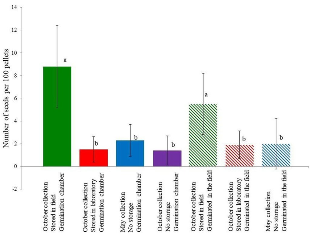
Figure 1. Number of seeds germinated per 100 cottontail fecal pellets ± standard deviation. Letters represent significant differences between treatments according to the Dunn test. Full bars represent treatments in germination chambers.
Discussion
The first experiment showed that seeds from both entire and disintegrated pellets can germinate equally well. We used disintegrated pellets in the following experiments because they are easier to homogeneously disperse in the experiment tray. However, germination was very low in the experiments with no soil. This suggests that if the pellets are placed on soil, the seeds inside are able to germinate, but if the cottontail forms a latrine on a rock or some other hard object (as it is commonly observed in our study location; pers. obs.), the pellets are not a good substrate for the plants to develop (at least in the fresh state). An interesting observation that we made was that in the October germination experiment, fungi were an important problem for plant development, but the same did not happen in the following experiment. This could be due to the fact that July-October are the months when most fungi expel their spores and infect the pellets (Valenzuela et al., 2009), but they apparently (at least partially) die before the germination period and by May do not represent an important threat for seeds or seedlings. Therefore, fungi are unlikely to strongly affect the process of seed dispersion by cottontails, since our October germination experiment would never happen in field conditions because of the dry season.
Baskin and Baskin (2014) mention that in xerophitic scrubs, 85% of seeds have some sort of dormancy; this is close to the results of our experiment. If we compare the number of seeds germinated from pellets stored in laboratory and field conditions, we can see that pellets exposed to the field yielded 5.9 (in germination chambers) and 2.9 (in the field) times more plants (Fig. 1). This suggests that most seeds have some sort of dormancy that is broken by the conditions in the field, most likely by heat, as it was shown for Opuntia tomentosa (Olvera-Carrillo et al., 2003). Notice that the Opuntia seeds almost never germinate after being stored in laboratory conditions (Table 1).
Table 1
Number and identity of the seeds germinated per 1,000 fecal pellets in each treatment. Chao estimator ± 95% confidence interval.
| Germinated in chambers | Germinated in the field | Total | |||||
| Collection | October collection | May collection | October collection | May collection | |||
| Storage | Field | Lab. | None | Field | Lab. | None | |
| Poaceae1 | 29 | 9 | 5 | 25 | 7 | 1 | 76 |
| Opuntia tomentosa | 13 | 1 | 14 | 12 | 0 | 17 | 57 |
| Physalis glutinosa | 15 | 2 | 2 | 8 | 7 | 2 | 36 |
| Jaegeria hirta | 17 | 1 | 0 | 8 | 2 | 0 | 28 |
| Drymaria laxiflora | 6 | 0 | 1 | 1 | 0 | 0 | 8 |
| Crusea longiflora | 5 | 0 | 0 | 0 | 0 | 0 | 5 |
| Jaltomata procumbens | 1 | 1 | 0 | 1 | 1 | 0 | 4 |
| Galinsoga parviflora | 1 | 0 | 0 | 0 | 0 | 0 | 1 |
| Evolvulus alsinoides | 1 | 0 | 0 | 0 | 0 | 0 | 1 |
| Bidens bigelovii | 0 | 0 | 0 | 0 | 1 | 0 | 1 |
| Solanum bulbocastanum | 0 | 1 | 0 | 0 | 0 | 0 | 1 |
| Buddleja cordata | 0 | 0 | 1 | 0 | 0 | 0 | 1 |
| Unidentified | 0 | 0 | 0 | 0 | 1 | 0 | 1 |
| Total seeds | 88 | 15 | 23 | 55 | 19 | 20 | 220 |
| Pellets used | 1,000 | 1,000 | 1,000 | 1,000 | 1,000 | 1,000 | 6,000 |
| Observed richness | 9 | 6 | 5 | 6 | 6 | 3 | 15 |
| Chao2 richness | 11.7 ± 4.1 | 10.6 ± 4.8 | 10.1 ± 6.5 | 7.9 ± 2.0 | 11.1 ± 6.5 | 3.5 ± 1.2 | 29.8 ± 13.4 |
1Includes: Aegopogon tenellus, Eragrostis Mexicana, and Chloris gayana (the last one is the only exotic species).
The Eastern cottontails showed to be poor seed dispersers if considering the amount of seeds per gram of excretes, 0.77 under the best conditions, compared with the 7.13 seeds/g of excrete dispersed by ringtails in the same location (Peña-Herrera et al., 2024). However, cottontails produce around 350 pellets/day (Cochran & Stains, 1961), which at a weight of 0.115 g/pellet (Glebskiy, 2016) which equals 40 g of excretes and thus up to 31 seeds dispersed per day per cottontail (and their population can rise up to 14 individuals/ha (Glebskiy, 2016). Another important consideration is the identity of the seeds, from the 14 species that we were able to identify; only 2 (Opuntia tomentosa and Buddleja cordata) could be considered dominant in the region (according to the list provided by Cano-Santana [1994]), and the other species are less common or even rare. Most noticeable Jaegeria hirta, which composes 12.7% of all seeds found and is a native but rare species for the location. It has to be noted that of the dispersed species (Table 1), only Chloris gayana is exotic to the location. When comparing to the seeds dispersed by ringtails in the same location (Peña-Herrera et al., 2024), we can see that only 3 species are shared (Opuntia tomentosa, Drymaria laxiflora, and Bidens sp.) and cottontails tend to disperse more Poaceae plants. This suggests that ringtails and rabbits have a complementary role as seed dispersers.
Therefore, we conclude that while being poor dispersers of seeds/g of excrete (the most commonly used estimator to measure dispersion efficiency), cottontails compensate for this by the sheer amount of excretes produced, their high population density, and the fact that they disperse mostly uncommon or even rare plants, and most are native to the region. Thus, cottontails are important seed dispersers and can have a great effect on some rare plants, especially Jaegeria hirta.
Acknowledgements
We are thankful to Díaz Rico A. and Zúñiga Ruíz B. for allowing us to use their germination chambers, Martínez Orea Y. for the plant identification, SEREPSA working team for the permits to collect pellets, List Sánches R. and Godínez Álvarez H. for their useful comments on this project, and Castellanos Vargas I. for technical support. This project was financially supported by PAPIIT grant IV200117 “Análisis ecosocial de una reserva urbana para la sustentabilidad en el campus de Ciudad Universitaria” to ZCS and a scholarship by Conacyt 817316 to YG.
References
Albert, A., Auffret, A. G., Cosyns, E., Cousins, S. A., D’hondt, B., Eichberg, C. et al. (2015). Seed dispersal by ungulates as an ecological filter: A trait-based meta-analysis. Oikos, 124, 1109–1120. https://doi.org/10.1111/oik.02512
Baskin, C. C., & Baskin, J. M. (2014). Seeds ecology, biogeography, and evolution of dormancy and germination. 2nd. Edition. San Diego: Elsevier.
Beaune, D., Bretagnolle, F., Bollache, L., Bourson, C., Hohmann, G., & Fruth, B. (2013). Ecological services performed by the bonobo (Pan paniscus): seed dispersal effectiveness in tropical forest. Journal of Tropical Ecology, 29, 367–380. https://doi.org/10.1017/S0266467413000515
Borchert, M., & Tyler, C. (2023). Fruit production and seed dispersal of Opuntia phaeacantha (Cactaceae) in the southwest Mojave Desert. Haseltonia, 29, 49–56. https://doi.org/10.2985/026.029.0108
Cano-Santana, Z. (1994). Flujo de energía a través de Sphenarium purpuracens(Orthoptera: Acrididae) y productividad primaria neta aérea en una comunidad xerófila. (Ph.D. Thesis). Mexico City: Universidad Nacional Autónoma de México.
César-García, S. F. (2002). Análisis de algunos factores que afectan la fenología reproductiva de la comunidad vegetal de la Reserva del Pedregal de San Ángel, D.F. (México) (Bachelor´s Thesis). Mexico City: Universidad Nacional Autónoma de México.
Chapman, J. A., & Flux, J. E. (2008). Introduction to the Lagomorpha. In P. C. Alves, N. Ferrand, & K. Hackländer (Eds.), Lagomorph Biology: evolution, ecology, and conservation (pp. 1–9). Berlin: Springer. https://doi.org/10.1007/978-3-540-72446-9
Chapman, J. A., Hockman, J. G., & Ojeda, C. M. M. (1980). Sylvilagus floridanus. Mammalian Species, 136, 1–8.
Cochran, G. A., & Stains, H. J. (1961). Deposition and decomposition of fecal pellets by cottontails. The Journal of Wildlife Management, 25, 432–435. https://doi.org/10.2307/3798835
Gelmi-Candusso, T. A., & Hämäläinen, A. M. (2019). Seeds and the city: the interdependence of zoochory and ecosystem dynamics in urban environments. Frontiers in Ecology and Evolution, 7, 41. https://doi.org/10.3389/fevo.2019.00041
Glebskiy, Y. (2016). Factores que afectan la distribución y abundancia del conejo castellano (Sylvilagus floridanus) en la Reserva del Pedregal de San Ángel, D.F. (México) (Bachekor’s Thesis). Mexico City: Universidad Nacional Autónoma de México.
Godó, L., Valkó, O., Borza, S., & Deák, B. (2022). A global review on the role of small rodents and lagomorphs (clade Glires) in seed dispersal and plant establishment. Global Ecology and Conservation, 33, e01982. https://doi.org/10.1016/j.gecco.2021.e01982
Hortelano-Moncada, Y., Cervantes, F. A., & Trejo-Ortiz, A. (2009). Mamíferos silvestres de la Reserva Ecológica del Pedregal de San Ángel en Ciudad Universitaria, Universidad Nacional Autónoma de México, México, D. F. Revista Mexicana de Biodiversidad, 80, 507–520. https://doi.org/10.22201/ib.20078706e.2009.002.614
Hudson, R., Rodríguez-Martínez, L., Distel, H., Cordero, C., Altbäcker, V., & Martínez-Gómez, M. (2005). A comparison between vegetation and diet records from the wet and dry season in the cottontail rabbit Sylvilagus floridanus at Ixtacuixtla, central Mexico. Acta Theriologica, 50, 377–389. https://doi.org/10.1007/BF03192633
Iluz, D. (2011). Zoochory: the dispersal of plants by animals. In Z. Dubinsky, & J. Seckbach (Eds.), All flesh is grass: plant-animal interrelationships (pp. 199–214). Dordrecht: Springer. https://doi.org/10.1007/978-90-481-9316-5_9
Lezama-Delgado, E., Sainos-Paredes, P., López-Portillo, J., Ángeles, G., Golubov, J., & Martínez, A. J. (2016). Association of Juniperus deppeana (Cupressaceae: Pinales) seeds with Mexican cottontail rabbit (Sylvilagus cunicularius; Leporidae: Lagomorpha) latrines. Journal of Natural History, 50, 2547–2555. https://doi.org/10.1080/
00222933.2016.1200685
Lorenzo, C., & Cervantes, F. (2005). Silvialgus floridanus. In G. C. G. Oliva, & G. Ceballos (Eds.), Los mamíferos silvestres de México. Mexico City: Comisión Nacional para el Conocimiento y Uso de la Biodiversidad/ Fondo de Cultura Económica.
Malo, J. E., & Suárez, F. (1995). Herbivorous mammals as seed dispersers in a Mediterranean dehesa. Oecologia, 104, 246–255. https://doi.org/10.1007/bf00328589
Olvera-Carrillo, Y., Márquez-Guzmán, J., Barradas, V. L., Sánchez-Coronado, M. E., & Orozco-Segovia, A. (2003). Germination of the hard seed coated Opuntia tomentosa
SD, cacti from the México valley. Journal of Arid Environments, 55, 29–42. https://doi.org/10.1016/s0140-1963(02)00268-9
Peña-Herrera, J. J., Glebskiy, Y., Hernández-Trejo, T., & Cano-Santana, Z. (2024). Ringtails (Bassariscus astutus) as seed dispersers in an urban gradient under conditions of low human activity due to COVID-19. Revista Mexicana de Biodiversidad, 95, e955351. https://doi.org/10.22201/ib.20078706e.2024.95.5351
Rosin, A. V., Gilio, N., & Meriggi, A. (2008). Introduced lagomorphs as a threat to “native” lagomorphs: the case of the Eastern cottontail (Sylvilagus floridanus) in northern Italy. In P. C. Alves, N. Ferrand, & K. Hackländer (Eds.), Lagomorph Biology: evolution, ecology, and conservation (pp. 153–164). Berlin: Springer. https://doi.org/10.1007/978-3-540-72446-9_11
Rzedowski, J. (1954). Vegetación del Pedregal de San Ángel. Anales de la Escuela Nacional de Ciencias Biológicas, Instituto Politécnico Nacional, 8, 59–129.
SMN (Servicio Meteorológico Nacional). (2025). Normales climatológicas 1991-2020, estación 9071 Colonia Educación. https://smn.conagua.gob.mx/tools/RESOURCES/Nor
males_Climatologicas/Normales9120/df/nor9120_09071.txt
Valenzuela, V. H., Herrera, T., & Pérez-Silva, E. (2009). Macromicetos. In A. Lot, & Z. Cano-Santana (Eds.), Biodiversidad del ecosistema del Pedregal de San Ángel (pp. 95–100). Mexico City: Universidad Nacional Autónoma de México.

Crecimiento, edad y tasa de mortalidad de la estrella de mar corona de espinas Acanthaster plancien el sur del golfo de California, México, durante un evento de explosión poblacional (2017-2018)
Growth, age and mortality rate of the crown-of-thorns starfish, Acanthaster planci, in the southern gulf of California, Mexico, during an outbreak event (2017-2018)
Héctor Reyes-Bonilla a, Frida J. Sánchez-Luna b, c, Luis E. Calderón-Aguilera d, *, Jenny Carolina Rodríguez-Villalobos e, f y María Dinorah Herrero-Pérezrul e
a Universidad Autónoma de Baja California Sur, Departamento Académico de Biología Marina, Carretera al sur Km 5.5, Col. El Mezquitito, 23090 La Paz, Baja California Sur, México
b Ghent University, Faculty of Sciences, Krijgslaan 281/N60, 9000 Gent, Bélgica
c Università Politecnica delle Marche, Via, Dipartimento di Scienze della Vita e dell’Ambiente, Brecce Bianche, 60131 Ancona, Italia
d Centro de Investigación Científica y de Educación Superior de Ensenada, Baja California, Carretera Tijuana – Ensenada 3918, 22860 Ensenada, Baja California, México
e Centro Interdisciplinario de Ciencias Marinas, Instituto Politécnico Nacional, Av. Instituto Politécnico Nacional s/n, Col. Playa Palo de Santa Rita, 23096 La Paz, Baja California Sur, México
f Ecosistemas y Conservación (Proazul Terrestre, A.C.), calle Héroes de Independencia 2440, 23000 La Paz, Baja California Sur, México
*Autor de correspondencia: leca@cicese.mx (L.E. Calderón-Aguilera)
Recibido: 18 febrero 2025; aceptado: 22 octubre 2025
Resumen
El asteroideo Acanthaster planci es un importante coralívoro y se requiere investigar en detalle aspectos de su ecología poblacional. El objetivo del estudio fue estimar parámetros demográficos de A. planci en el archipiélago Espíritu Santo, golfo de California. Entre julio 2017 y octubre 2018 se midió el diámetro del disco de 356 especímenes y con base en análisis de frecuencia de tallas, se calculó el diámetro de disco máximo teórico, la tasa de crecimiento y mortalidad, y la longevidad de la población. El tamaño máximo del disco fue de 30.8 cm, la tasa de crecimiento de 0.429/año, la longevidad de 6 años y la tasa de mortalidad fue de 1.039/año. La edad de los individuos revisados en 2017 fluctuó entre 1.0 y 1.25 años, y en 2018 fue de 1.75 a 2.25 años, lo que sugiere que la cohorte de 2016 causó el notable aumento poblacional registrado para A. planci en 2017. Este evento pudo haber resultado de la combinación del alto reclutamiento larval favorecido por el agua cálida aportada por el evento de El Niño de 2015 y una alta sobrevivencia de juveniles debido a la presencia de abundante alimento algal como consecuencia de La Niña en 2016.
Palabras clave: Frecuencia de tallas; FISAT; Mortalidad; Crecimiento; Reclutamiento; Brote poblacional
Abstract
The asteroid Acanthaster planci is an important corallivore, and the investigation of some aspects of its population ecology are required. The objective of this study was to estimate demographic parameters of A. planci at Espíritu Santo Archipelago, Gulf of California. Between July 2017 and October 2018, the disk diameter of 356 specimens was measured, and with these data the theoretical maximum diameter, growth and mortality rates, and longevity of the population were estimated on the basis of size frequency analyses. The maximum disk size was 30.8 cm, growth rate was 0.429 yr-1, longevity was 6 years, and mortality rate was 1.039 yr-1. Age of the individuals assessed in 2017 fluctuated between 1.0 and 1.25 years, and in 2018 was from 1.75 to 2.25 years, which suggests that the 2016 cohort caused a noteworthy population to increase recorded for A. planci in 2017. This event may have resulted from the combination of high larval recruitment favored by the warm water brought by the 2015 El Niño, and high juvenile survival due to abundant algal food as consequence of La Niña in 2016.
Keywords: Length frequency; FISAT; Mortality; Growth; Recruitment; Outbreak
Introducción
La estrella corona de espinas (Acanthaster spp.) es uno de los equinodermos que ha sido más estudiado en arrecifes del Indo-Pacífico debido al interés que genera el incremento excesivo en la densidad de sus poblaciones. Cuando ésto ocurre, la intensidad de la depredación de la estrella sobre los corales supera las tasas de crecimiento de las colonias y el asteroideo se convierte en una de las mayores amenazas para los arrecifes coralinos (De’ath et al., 2012; Kayal et al., 2012; Pratchett et al., 2014). Hasta la fecha (septiembre 2025), de acuerdo con el Registro Mundial de Especies Marinas (World Register of Marine Species; WoRMS: https://www.marinespecies.org/aphia.php?p=taxdetailsyid=205212), se reconocen 4 especies pertenecientes al género Acanthaster: A. planci (Linneo, 1758), A. mauritiensis de Loriol, 1885, A. brevispinus, Fisher, 1917 y A. benziei Worheide, Kaltenbaher, Cowan y Hazprunar, 2022, aunque estudios genéticos apuntan a que A. planci en realidad es un complejo de posiblemente 5 taxones (Hazprunar y Spies, 2014), y refieren que la especie presente en la costa del Pacífico de América podría ser Acanthaster sp. cf. solaris Schreber, 1793. Aunque este último nombre se ha usado en publicaciones recientes relativas a la ecología de Acanthaster en el Pacífico oriental (Martínez-Sarabia y Reyes-Bonilla, 2021; Rodríguez-Villalobos y Ayala-Bocos, 2018, 2021), la discusión sigue activa y por motivos de estabilidad taxonómica, en el presente trabajo se decidió utilizar el nombre de A. planci para referirse a la especie de interés.
A pesar de su presencia en los arrecifes rocosos y coralinos de la región del Pacífico oriental tropical, la estrella no ha recibido demasiada atención quizás debido a sus densidades relativamente bajas (Enochs y Glynn, 2017; Reyes-Bonilla y Calderón-Aguilera, 1999; Rodríguez-Villalobos et al., 2016), así como a la poca evidencia de daño masivo sobre los corales (Rodríguez-Villalobos et al., 2015). Sin embargo, Rodríguez-Villalobos y Ayala-Bocos (2018, 2021) señalaron que en 2017 hubo un incremento abrupto en la densidad de los individuos de esta especie en el Parque Nacional Zona Marina del Archipiélago Espíritu Santo (PNZMAES) acompañado por la mortalidad masiva de colonias de coral de los géneros Pocillopora, Porites y Pavona. Este evento tuvo efectos importantes sobre las comunidades coralinas e incluso afectó esfuerzos de restauración que se estaban llevando a cabo en la misma región (Martínez-Sarabia y Reyes-Bonilla, 2021).
Las causas del incremento de A. planci en el sur del golfo de California son desconocidas. En el Indo-Pacífico las fluctuaciones del tamaño de la población de la estrella se han relacionado con condiciones ambientales como aumentos de temperatura, alta concentración de clorofila y baja salinidad (Fabricius et al., 2010; Hoegh-Guldberg y Pearse, 1995; Lamare et al.,2014). Aunque hasta el momento no hay una explicación universal para la formación de brotes poblacionales (Babcock et al., 2016), el fenómeno debe estar relacionado con las características biológicas de la estrella, tales como alto potencial reproductivo y fecundidad, buena sobrevivencia larval y reclutamiento de individuos, sistemas defensivos en su fase adulta (que incluyen espinas, saponinas y compuestos alelopáticos), y alta capacidad competitiva; además, existen pocos depredadores naturales que controlen el crecimiento de sus poblaciones (Pratchett et al., 2014).
A partir de la observación del aumento anómalo de su abundancia en la región sur del golfo de California y para tener mejores herramientas para el manejo del problema, surgió la interrogante de conocer la estructura de edades de A. planci en la región para elucidar la posible relación del incremento de abundancia con un pulso previo de alto reclutamiento. Así, el objetivo de este trabajo fue obtener los parámetros de la ecuación de crecimiento para una población de A. planci en fase explosiva y calcular la edad relativa de los organismos, además de la tasa de mortalidad natural.
Materiales y métodos
El archipiélago Espíritu Santo se encuentra al oriente de la bahía de La Paz (24º28’17” N, 110º19’57” O; fig. 1). Topográficamente, el litoral oriental de la isla es rocoso y homogéneo, mientras que la costa occidental cuenta con entrantes y salientes que forman zonas protegidas. Las zonas someras en el lado oeste de Espíritu Santo permiten la formación de arrecifes rocosos con la presencia de parches coralinos distribuidos de manera discontinua (Reyes-Bonilla y López-Pérez, 2009). Se registran temperaturas mínimas de 20 ºC a finales del invierno (febrero) y máximas de 30 ºC a mediados del verano (agosto). Adicionalmente, se observan corrientes de menor intensidad en la parte norte y de mayor intensidad en la parte sur (canal de San Lorenzo) (Conanp, 2018).
Se visitaron 10 localidades en el archipiélago (fig. 1) en julio y agosto de 2017, y en septiembre y octubre de 2018 para determinar la abundancia y el diámetro del disco (en cm) de todos los ejemplares de la estrella que se encontraban dentro de transectos de banda de 25 x 3 m, desplegados en paralelo a la línea de costa a una profundidad de 2 a 10 m. Para estimar la tasa de crecimiento y de mortalidad, se empleó el paquete FISAT II (FAO-ICLARM Fish Stock Assessment Tools versión 1.2.2). Se decidió aplicar la curva de crecimiento de von Bertalanffy (Haddon, 2011), ya que Pratchet et al. (2014), después de un análisis de los diversos trabajos al respecto, indican que este es el modelo que mejor expresa el crecimiento de Acanthaster a partir del segundo año de vida.
Para la aplicación del modelo, la talla máxima teórica L∞ fue calculada empleando la técnica de Powell-Wetherall (Haddon, 2011), la cual parte de la suposición que la población está en estado estable (tasa de mortalidad proporcional a la tasa de reclutamiento), y se fundamenta en las siguientes ecuaciones:
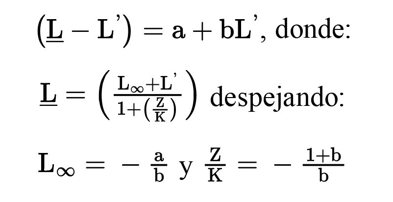
Por otra parte, la tasa de crecimiento K se obtuvo con el método de Shepherd (Haddon, 2011), el cual busca maximizar una función no paramétrica S, que se define como
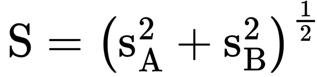
donde SAy SB son los valores de bondad de ajuste (“scores”) obtenidos en tiempo calendario (stz) para SA = 0 y SB = 0.25 años a partir del origen de la curva de crecimiento de VB. Las ecuaciones aplicadas son:
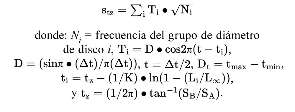
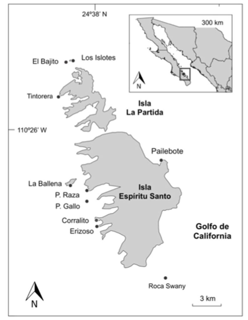
Figura 1. Localización de los puntos de muestreo para la determinación de tallas de Acanthaster planci en el Parque Nacional Zona Marina del Archipiélago Espíritu Santo (PNZMAES).
Una vez con los parámetros L∞ y K, se procedió a trazar la curva teórica de crecimiento de la especie (expresando el diámetro en cm en relación con la edad del organismo en intervalos de 0.25 años) a construir la tabla diámetro de disco-edad, con lo cual se determinó la edad de los individuos muestreados en 2017 y 2018. Tomando en cuenta que los estudios previos sobre crecimiento de la estrella corona de espinas han sido hechos con base en el diámetro total de los individuos (Zann et al., 1987), se trazó una curva teórica para evaluar el crecimiento en esta dimensión, considerando que Glynn (1982) determinó que el diámetro total de Acanthaster en Panamá podría ser aproximado a partir del diámetro del disco ya que este representa 56% del total.
Finalmente, para calcular la tasa de mortalidad de la población (M) de especies a las que no se les puede asignar directamente la edad con base en estructuras óseas u otros procedimientos, se emplean ecuaciones empíricas o basadas en aspectos teóricos del crecimiento de organismos marinos (Sparre y Venema, 1995). La bibliografía cita el uso de diversas metodologías para evaluar este parámetro en equinodermos comerciales (Herrero-Pérezrul y Chávez, 2005; Reyes-Bonilla y Herrero-Pérezrul, 2003), pero para el caso de Acanthaster no todas son aplicables ya que su uso requiere información no disponible; por ejemplo, la ecuación de Rikhter y Efanov utilizada por Penchaszadeh y Molinet (2020), necesita la edad de primera madurez (la cual es desconocida para Acanthaster en el Pacífico americano), mientras que métodos como el de Beverton y Holt (Sparre y Venema, 1995) solo son aplicables a especies de consumo humano porque requieren datos de talla de primera captura. Por lo anterior, se decidió estimar valores de M usando 3 métodos: la ecuación de Pauly (1984) basada en la temperatura promedio local (25 °C) y el valor de L∞ y K; la de Jensen (1997), fundamentada en el valor de K; y la curva de captura de Ricker (1975), obtenida de la frecuencia de individuos y sus respectivas edades estimadas.
Resultados
Se midieron 356 individuos de A. planci en 2017 y 2018. Los especímenes de 2017 fueron en promedio 5.5 cm más pequeños que los de 2018 (tabla 1, fig. 2; t de Student para varianzas desiguales t318 = 13.413, p < 0.001). La distribución de tallas de los individuos se presenta en las figuras 2 y 3, y puede observarse que en 2017 solamente un individuo alcanzó un diámetro de disco superior a 20 cm, mientras que en el año siguiente 21 de 227 organismos (9.3%) superan ese umbral. En 2017, 9% de las estrellas fueron menores a 8 cm de diámetro.
A partir de los análisis de tallas, el diámetro máximo de disco estimado para la población de Acanthaster estudiada (L∞) fue de 30.8 cm mientras que su tasa anual de crecimiento (K) fue de 0.429∙año-1. La ecuación de crecimiento toma entonces la siguiente forma:
Lt = 30.8 * (1 – e [-0.429* (t – 0.01)]),
donde: Lt = diámetro de disco (en cm) a la edad t y t = edad (años).
Los organismos crecen rápidamente de tal modo que al final del año 1 cuentan con 10.7 cm de diámetro de disco, para el año 2 alcanzan 17.7 cm, y para el 3 llegan a 22.2 cm. El modelo teórico junto con la edad estimada de los individuos se presenta en la figura 4. Para facilitar comparaciones con otras publicaciones donde se hace referencia a la talla de A. planci en el Pacífico americano y donde la medida de los organismos se hizo tomando en cuenta el diámetro total, en la figura 5 se presenta la curva teórica de crecimiento aquí generada y la esperada para el diámetro total, considerando que el diámetro del disco representa 55% del diámetro total de la estrella según Glynn (1982).
La estructura esperada de edades para los años 2017 y 2018 a partir de la ecuación de von Bertalanffy y calculada con el diámetro del disco, se presenta en la figura 6. Se observa que la edad predominante en el primer año de muestreo fue entre 1 y 1.5 años (a partir de julio), indicando que los individuos posiblemente se reclutaron a finales de 2015. Esto es corroborado en la figura 6, ya que para 2018 hubo una alta frecuencia de animales con edades de 1.75 a 2.25 años.
Tabla 1
Estadísticos descriptivos (en cm) del diámetro del disco de la población de Acanthaster planci estudiada en el Parque Nacional Zona Marina del Archipiélago Espíritu Santo (PNZMAES) en 2017 y 2018.
| Estadístico | 2017 | 2018 | Ambos años |
| Promedio | 11.43 | 16.96 | 14.96 |
| Desviación típica | 5.44 | 4.28 | 4.78 |
| Error típico | 0.29 | 0.23 | 0.25 |
| Moda | 11 | 16 | 16.0 |
| Mediana | 10.9 | 16.5 | 15.0 |
| Máximo | 23.3 | 28.0 | 28.0 |
| Mínimo | 3.8 | 5.2 | 3.8 |
| N | 129 | 227 | 356 |
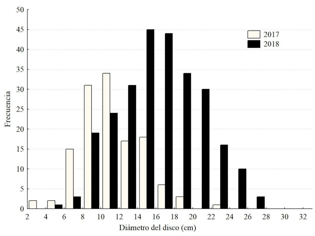
Figura 2. Histogramas del diámetro del disco (en cm) para la población de Acanthaster planci en el Parque Nacional Zona Marina del Archipiélago Espíritu Santo (PNZMAES) durante los años 2017 y 2018.
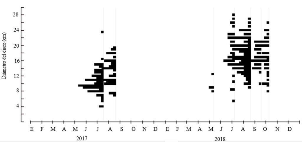
Figura 3. Frecuencia de diámetro del disco de Acanthaster planci en el Parque Nacional Zona Marina del Archipiélago Espíritu Santo (PNZMAES) durante los años 2017 y 2018.
Por último, la tasa anual de mortalidad esperada para la población de A. planci analizada, dependiendo del método indirecto aplicado, fue de 1.0392 (ecuación de Pauly), 0.3983 (curva de captura) y 0.6433 (ecuación de Jensen), con un promedio de 0.6936∙año-1. La mortalidad en el año 1 es alta, ya que el método que arrojó los valores más conservadores (Ricker) indica pérdidas de 33% de la cohorte teórica, mientras que el método de Pauly indica que apenas sobrevive 35%. Al tomar en cuenta el valor promedio de las 3 estimaciones del parámetro M, para el año 1 sobrevive 49.9% de la cohorte, para el año 3 apenas 12.5% de los individuos originales permanece y solo 3.1% alcanza la edad de 5 años. Estos valores se reflejan en los histogramas de edad (fig. 6) donde la edad máxima observada (5.75 años) fue de un individuo de 28 cm.
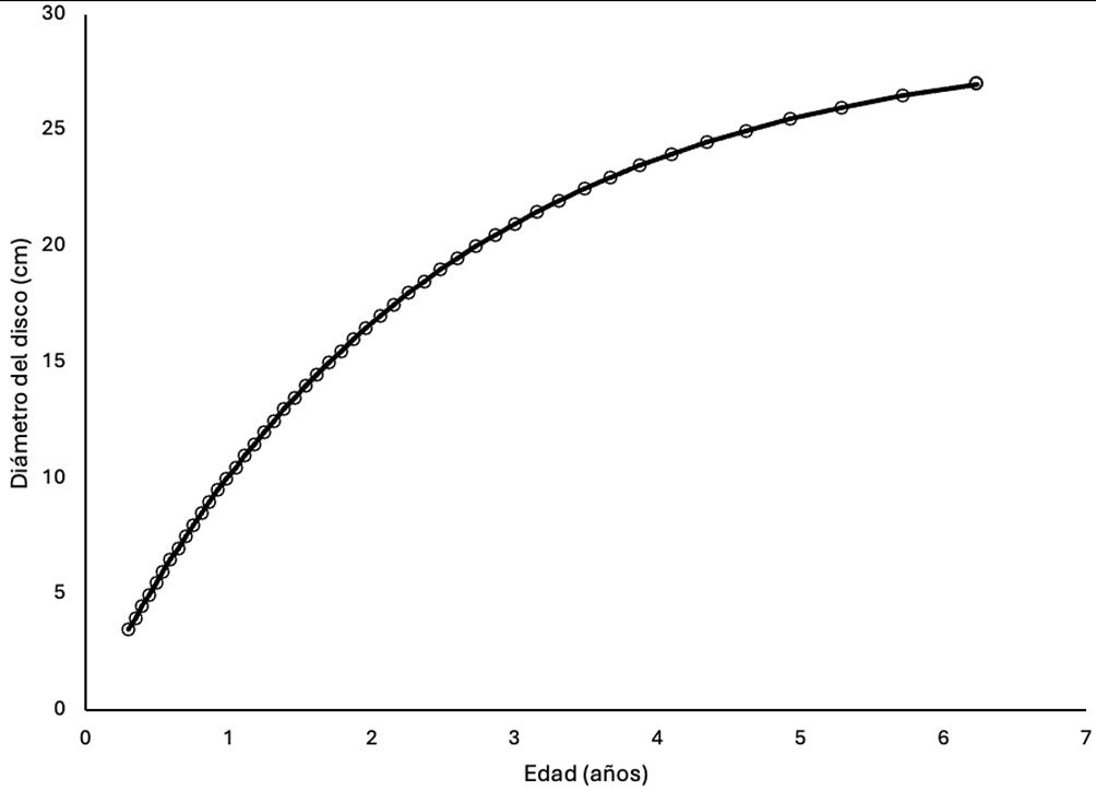
Figura 4. Curva talla-edad de Acanthaster planci en el Parque Nacional Zona Marina del Archipiélago Espíritu Santo (PNZMAES, n = 356).
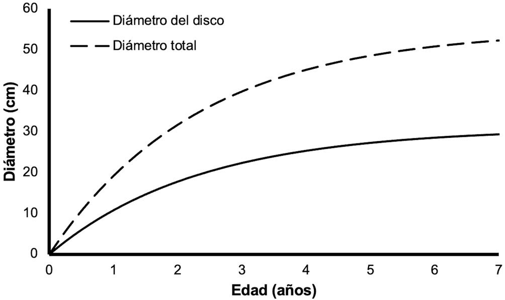
Figura 5. Curvas de crecimiento individual de Acanthaster planci en el Parque Nacional Zona Marina del Archipiélago Espíritu Santo (PNZMAES). La línea puntuada representa la curva extrapolada a partir de la ecuación de Glynn (1982).
Discusión
Este es el primer estudio de crecimiento de Acanthaster planci en el Pacífico oriental y uno de los pocos a escala mundial (MacNeil et al., 2017; Pratchett et al., 2014; Zann et al., 1987). El cálculo de los parámetros de crecimiento de esta especie ha sido difícil de realizar especialmente porque los marcajes en campo para hacer seguimiento de tallas a lo largo del tiempo no han sido exitosos, ya que los individuos eliminan los colorantes o autotomizan la espina o incluso el brazo donde se coloca la marca (Chim y Tan, 2013; MacNeil et al., 2016; Pratchett et al., 2014). Además, en el caso del continente americano, otro motivo que hace complicado conducir estudios demográficos es que las poblaciones son relativamente pequeñas (menos de 70 ind/ha, equivalente a encontrar 1 individuo cada 142.8 m2, según Rodríguez-Villalobos et al. [2021]), lo cual hace complejo tener tamaños de muestra adecuados para realizar análisis en detalle.
Para solucionar ésto, la mayor parte de los trabajos sobre crecimiento de Acanthaster se han basado en especímenes mantenidos en confinamiento (Lucas, 1984; Yamaguchi, 1974; Zann et al., 1987), pero por las dificultades logísticas que implica mantener ejemplares a largo plazo, los experimentos no han durado más de 1 o 2 años. Otra opción para estimar la edad de Acanthaster ha sido la relación entre el número de anillos de las espinas (tomado como indicador indirecto de la edad) y el diámetro total medido en el campo (MacNeil et al., 2017; Stump, 1996), pero la debilidad de estos estudios radica en que no se ha logrado demostrar que los anillos sean anuales. Finalmente, Kenchington (1977) empleó información de 10 años de mediciones de organismos en la Gran Barrera Arrecifal y a partir de cambios en las modas estimó que a la edad de 3 años un individuo podrá superar los 30 cm de diámetro máximo; es decir, el autor empleó un método indirecto similar al utilizado en el presente trabajo. En resumen, los métodos empleados en esta investigación permiten alcanzar estimaciones de crecimiento con una precisión muy semejante a las que se han obtenido en otras partes del mundo, por lo que los resultados obtenidos son confiables.
La talla promedio que se observó tomando en cuenta los años 2017 y 2018 (14.96 + 0.25 cm; tabla 1) frecuentemente se observa en individuos residentes de los arrecifes del Pacífico oriental tropical (Glynn, 1982; Narváez y Zapata, 2010), pero muy inferior a la que se alcanza en el Indo-Pacífico (MacNeil et al., 2016; Mendonça et al., 2010). Esta diferencia se puede explicar con base en los argumentos de Kettle y Lucas (1987) y Hernández-Morales et al. (2021), quienes anotan que la talla de Acanthaster es proporcional a la calidad del alimento consumido, por lo que el pequeño tamaño de los individuos en la zona de estudio y a lo largo del Pacífico oriental tropical se puede deber a que las poblaciones de la estrella corona de espinas tienen una dieta pobre, probablemente debido a que la cobertura y diversidad de corales para alimentarse es mucho menor que en el resto del Pacífico.
Aunque existen diferencias notables tanto en las tallas alcanzadas por Acanthaster en distintas regiones como en las metodologías aplicadas para determinar su curva de crecimiento, los estudios llevados a cabo en Australia muestran que en el primer año de vida esta especie normalmente no alcanza los 5 cm de diámetro total, pero su crecimiento es muy rápido durante el segundo año, alcanzando entre 12.5 y 25 cm, y para el año 3 puede llegar a los 35 cm de diámetro máximo (MacNeil et al., 2017; Pratchett et al., 2014; Zann et al., 1987). Estos hallazgos presentan cierta discrepancia en relación con la talla esperada en el archipiélago Espíritu Santo a un año (fig. 5), la cual es de más de 19 cm de diámetro total, de acuerdo con la corrección sugerida por Glynn (1982). Kenchington (1977), empleando un método de progresión modal, también sugirió que Acanthaster puede alcanzar hasta 12 cm de diámetro máximo para el año 1, pero esa cifra sigue siendo baja comparada con la aquí presentada. Considerando lo anterior, es posible que, como sugieren Pratchett et al. (2014), aunque el modelo de crecimiento de von Bertalanffy es robusto en general y aplicable para describir la relación entre talla y edad de organismos adultos de Acanthaster, no es muy apropiado para determinar la edad de individuos pequeños. Esto se debe a que durante su primer año, la estrella corona de espinas tiene tasas lentas de desarrollo debido a que se alimenta principalmente de algas (Kamya et al., 2017); posteriormente, pasando los 10 cm de diámetro (año 2), los ejemplares comienzan a alimentarse de coral y aceleran notablemente su crecimiento, de acuerdo con Kettle y Lucas (1987).
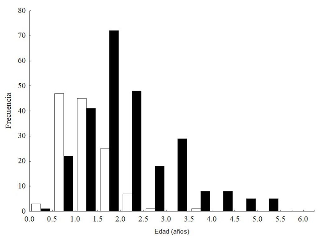
Figura 6. Estructura de edades calculada para los individuos de Acanthaster planci muestreados en 2017 y 2018 en el Parque Nacional Zona Marina de la Isla Espíritu Santo (PNZMAES).
La tasa anual de crecimiento encontrada (K) en este estudio fue de 0.429 año-1, muy similar a la reportada por MacNeil et al. (2017) de 0.54. Los valores en sí no son comparables dado que se emplearon distintas metodologías, por lo que la discusión no puede extenderse más allá de denotar la similitud. Por otra parte, la talla máxima teórica (L∞) del disco de Acanthaster en el PNZMAES fue de 30.8 cm, cercana a la presentada por MacNeil et al. (2017) de 34.9 cm a partir de un modelo bayesiano de Bertalanffy y ambas son mucho más altas que la de 20.2 cm reportada por Zann et al. (1987) en condiciones experimentales y con individuos a los que se les proporcionaron dietas de baja calidad. Usando el factor de corrección propuesto por Glynn (1982), el disco de 30.8 cm se traduce a un diámetro total de 56 cm y ello indica que teóricamente los ejemplares del golfo de California pueden alcanzar los tamaños registrados por Stump (1996) y Pan et al. (2010) en Australia y Japón (58 y 47.4 cm, respectivamente) y por Byrne et al. (2017) en la Gran Barrera Arrecifal (40 cm pero hasta 70 cm de diámetro máximo).
Además de generar el modelo de crecimiento, otro objetivo de este trabajo fue generar insumos para tratar de explicar la causa del fenómeno de explosión poblacional observado para Acanthaster en el PNZMAES durante 2017 y 2018. A este respecto y con base en la relación talla-edad, los histogramas (fig. 6) muestran que el reclutamiento de los individuos debió haber ocurrido en 2015, año durante el cual la zona se vio impactada por uno de los eventos de oscilación sureña de El Niño más fuertes en lo que va del siglo XXI y el cual afectó a los arrecifes de coral del Pacífico oriental y a las especies asociadas (Cruz-García et al., 2020; Riegl et al., 2019). La anomalía térmica alcanzada en la región de la bahía de La Paz fue superior a 2 °C (Coria-Monter et al., 2018) y alteró la ecología de todo tipo de organismos, desde mamíferos marinos hasta elementos del plancton (Elorriaga-Verplancken et al., 2016; Portner et al., 2022). Por el contrario, al año siguiente (2016-2017) la región del golfo de California estuvo influenciada por un evento de La Niña que favoreció la alta concentración de clorofila a en la columna de agua, la presencia de surgencias y aumentó la productividad (Farach-Espinosa et al., 2021).
Considerando lo anterior, es posible hipotetizar las causas del evento de explosión poblacional. Dado que las altas temperaturas aumentan la sobrevivencia larval y de los juveniles de Acanthaster (Hughes et al., 2014; Lamare et al., 2014, Pratchett et al., 2017), las anomalías térmicas de la región sur del golfo de California en 2015, combinadas con la enorme fecundidad de la estrella (más de 50 millones de huevos por individuo; Conand, 1984; Hughes et al., 2014), debieron favorecer un reclutamiento masivo. Posteriormente, las condiciones frías y productivas en el año 2016 pudieron aumentar la sobrevivencia de los juveniles al impulsar un mejor crecimiento algal en el fondo arrecifal (Wolfe et al., 2017). Así, para el año 2017 los organismos ya tenían tallas fácilmente detectables en el campo y comenzaron a realizar sus actividades de depredación, las cuales causaron notables daños a las comunidades de coral de la zona de estudio ese año (Rodríguez-Villalobos y Ayala-Bocos, 2018).
La hipótesis anterior se sustenta por los datos del modelo de edad y también por las tallas observadas en el campo. Los diámetros de disco esperados para los ejemplares (promedios de 11.43 ± 0.29 cm en 2017 y 16.96 ± 0.23 cm en 2018; tabla 1) coinciden con los reportados por Rodríguez-Villalobos y Ayala-Bocos (2021) para la zona de El Corralito en la isla Espíritu Santo (fig. 1) en 2017 (14.72 ± 2.85 cm de diámetro), lo que indica que para ese año la población de Acanthaster en la zona de estudio estaba compuesta fundamentalmente de individuos menores a 3 años, nacidos en 2015-2016 (fig. 6).
Finalmente, el modelo de sobrevivencia indica que un porcentaje muy elevado de los reclutas desaparece en el primer año de vida. Varios estudios han indicado que la tasa de mortalidad de los juveniles de Acanthaster es muy elevada (Fabricius et al., 2010; Nakamura et al., 2014; Zann et al., 1987), aunque la estimación en campo de este parámetro es notablemente difícil de obtener ya que los individuos recién reclutados de la estrella son crípticos (Fabricius, 2013). La longevidad esperada en el archipiélago Espíritu Santo fue de aproximadamente 6 años, lo cual corresponde bien a lo reportado por otros autores en Australia que indican entre 4 y 9 años de vida (Lucas, 1984; Pratchett et al., 2014). Tomando en cuenta este dato clave, es probable que la mayor parte de la cohorte de 2015 que causó el evento de mortalidad coralina masiva ya no estuviera presente en los arrecifes de la zona de estudio después del año 2021, lo cual fue confirmado a partir de datos de censos (densidades de 0.27 ind/50m2 en 2017-2018 bajó a 0.19 ind/50m2 en 2023-24). Esto implica que la población de la estrella de mar corona de espinas en el sur del golfo de California se comportó siguiendo el modelo de “aumento-caída”, típico de la especie en el Indo-Pacífico y de otros equinodermos con larvas planctotróficas (Uthicke et al., 2009).
Agradecimientos
A las autoridades y el personal del PNZMAES por las facilidades logísticas. A los miembros del staff y estudiantes asociados a la Sociedad de Historia Natural Niparajá, A.C., al personal del Laboratorio de Sistemas Arrecifales (UABCS) y a Arturo Ayala Bocos que apoyaron en las labores de campo. Las observaciones y comentarios de un revisor anónimo y del editor de la Revista Mexicana de Biodiversidad fueron clave para mejorar la presentación de las ideas y fortalecer la calidad del manuscrito.
Referencias
Babcock, R. C., Dambacher, J. M., Morello, E. B., Plagányi, É. E., Hayes, K. R., Sweatman, H. P. A. et al. (2016). Assessing different causes of Crown-of-Thorns starfish outbreaks and appropriate responses for management on the Great Barrier Reef. Plos One, 11, e0169048. https://doi.org/10.1371/journal.pone.0169048
Barham, E. G., Gowdy, R. W. y Wolfson, F. H. (1973). Acanthaster (Echinodermata, Asteroidea) in the Gulf of California. Fishery Bulletin, 71, 927–942.
Byrne, M., Rowe, F. W., Marsh, M. L. y Mah, L. C. (2017). Class Asteroidea. En: O’Hara, T. y Byrne, M. (Eds.), Australian echinoderms: biology, ecology and evolution (pp. 231–294). Melbourne: CSIRO publishing, Clayton South, Australia.
Chim, C. K. y Tan, K. S. (2013). A method for the external attachment of acoustic tags on sea stars. Journal of the Marine Biology Association of the United Kingdom, 93, 267–272. https://doi.org/10.1017/S0025315411002128
Conanp (Comisión Nacional de Áreas Naturales Protegidas). (2018). Programa de Manejo Parque Nacional exclusivamente la zona marina del Archipiélago de Espíritu Santo. Disponible en: https://www.gob.mx/publicaciones/es/articulos/parque-nacional-exclusivamente-la-zona-marina-del-archipielago-de-espiritu-santo?idiom=es
Conand, C. (1984). Distribution, reproductive cycle and morphometric relationships of Acanthaster planci (Echinodermata: Asteroidea) in New Caledonia, western tropical Pacific. Proceedings of the 5th International Echinoderm Conference, Galway, 1, 499–506.
Coria-Monter, E., Monreal-Gómez, M. A., de León, D. A. S. y Durán-Campos, E. (2018). Impact of the “Godzilla El Niño” Event of 2015-2016 on sea-surface temperature and chlorophyll-a in the southern Gulf of California, Mexico, as evidenced by satellite and in situ data. Pacific Science, 72, 411–422. https://doi.org/10.2984/72.4.2
Cruz-García, R., Rodríguez-Troncoso, A. P., Rodríguez-Zaragoza, F. A., Mayfield, A. y Cupul-Magaña, A. L. (2020). Ephemeral effects of El Niño southern oscillation events on an eastern tropical Pacific coral community. Marine Freshwater Research, 71, 1259–1268. https://doi.org/10.1071/MF18481
Dana, T. y Wolfson, A. (1970). Eastern Pacific Crown-of-thorns starfish populations in the lower Gulf of California. San Diego Society of Natural History, 16, 83–90. https://doi.org/10.5962/bhl.part.15455
De’ath G., Fabricius, K. E., Sweatman, H. y Puotinen, M. (2012). The 27-year decline of coral cover on the Great Barrier Reef and its causes. Proceedings of the National Academy of Sciences of the Unites States of America, 109, 17995–17999. https://doi.org/10.1073/pnas.1208909109
Elorriaga-Verplancken, F. R., Rosales-Nanduca, H. y Robles-Hernández, R. (2016). Unprecedented records of Guadalupe fur seals in La Paz Bay, Southern Gulf of California, Mexico, as a possible result of warming conditions in the northeastern Pacific. Aquatic Mammals, 42, 261–267. https://doi.org/10.1578/AM.42.3.2016.261
Enochs, I. C. y Glynn, P. W. (2016). Corallivory in the eastern Pacific. En Glynn, P. W., Manzello, D. y Enochs, I. C. (Eds.), Coral reefs of the Eastern Tropical Pacific: persistence and loss in a dynamic environment (pp. 315–337). Dordrecht: Springer Netherlands. https://doi.org/10.1007/978-94-017-7499-4_10
Fabricius, K. (2013). Acanthaster planci. En J. M. Lawrence (Eds.), Starfish: Biology and ecology of the Asteroidea (pp. 132–141). Baltimore: The Johns Hopkins University Press.
Fabricius, K. E., Okaji, K. y De’ath, G. (2010) Three lines of evidence to link outbreaks of the crown-of-thorns sea star Acanthaster planci to the release of larval food limitation. Coral Reefs, 29, 593–605. https://doi.org/10.1007/s00338-010-0628-z
Farach-Espinoza, E. B., López-Martínez, J., García-Morales, R., Nevárez-Martínez, M. O., Lluch-Cota, D. B. y Ortega-García, S. (2021). Temporal variability of oceanic mesoscale events in the Gulf of California. Remote Sensing, 13, 1774. https://doi.org/10.3390/rs13091774
Fisheries and aquaculture software. FISAT II – FAO-ICLARM Stock Assessment Tool. En FAO Fisheries and Aquaculture Department (online). Rome. Recuperado 20 agosto, 2025 de: https://www.fao.org/fishery
Glynn, P. W. (1982). Individual recognition and phenotypic variability in Acanthaster planci (Echinodermata: Asteroidea). Coral Reefs, 1, 89–94. https://doi.org/10.1007/BF00301690
Haddon, M. (2011). Modelling and quantitative methods in fisheries, 2° Ed. San Francisco: Chapman y Hall.
Haszprunar, G. y Spies, M. (2014). An integrative approach to the taxonomy of the crown-of-thorns starfish species group (Asteroidea: Acanthaster): a review of names and comparison to recent molecular data. Zootaxa, 3841, 271–284. https://doi.org/10.11646/zootaxa.3841.2.6
Hernández-Morales, A., Herrero-Pérezrul, M. D. y Vázquez-Arce, D. I. (2021). Variability of size and food type of Acanthaster planci (Echinodermata: Asteroidea) in the southern Gulf of California, Mexico. Revista de Biología Tropical, 69, 185–201. https://doi.org/10.15517/rbt.v69iSuppl.1.46352
Herrero-Pérezrul, M. D. y Chávez, E. A. (2005). Optimum fishing strategies for Isostichopus fuscus (Echinodermata: Holothuroidea) in the Gulf of California, México. Revista de Biología Tropical, 53 (Suppl. 3), 357–366.
Hoegh-Guldberg, O. y Pearse, J. S. (1995). Temperature, food availability, and the development of marine invertebrate larvae. American Zoologist, 35, 415–425.
Hughes, R. N., Hughes, D. J. y Smith, I. P. (2014). Limits to understanding and managing outbreaks of crown-of-thorns starfish (Acanthaster spp.). Oceanography and Marine Biology Annual Review, 52, 133–200. https://doi.org/10.1201/b17143-4
Jensen, A. L. (1997). Origin of the relation between K and Linf and synthesis of relations among life history parameters. Canadian Journal of Fisheries and Aquatic Sciences, 54,987–989. https://doi.org/10.1139/f97-007
Kamya, P. Z., Byrne, M., Mos, B., Hall, L. y Dworjanyn, S. A. (2017). Indirect effects of ocean acidification drive feeding and growth of juvenile crown-of-thorns starfish, Acanthaster planci. Proceedings of the Royal Society of Biology, 284, 20170778. https://doi.org/10.1098/rspb.2017.0778
Kayal, M., Vercelloni, J., Lison de Loma, T., Bosserelle, P., Chancerelle, Y., Geoffroy, S. et al. (2012). Predator Crown-of-Thorns starfish (Acanthaster planci) outbreak, mass mortality of corals, and cascading effects on reef fish and benthic communities. Plos One, 7, e47363. https://doi.org/10.1371/journal.pone.0047363
Kenchington, R. A. (1977). Growth and recruitment of Acanthaster planci (L.) on the Great Barrier Reef. Biological Conservation, 11, 103–118. https://doi.org/10.1016/0006-3207(77)90032-5
Kettle, B. T. y Lucas, J. S. (1987). Biometric relationships between organ indices, fecundity, oxygen consumption and body size in Acanthaster planci (L.) (Echinodermata; Asteroidea). Bulletin of Marine Science, 41, 541–551.
Lamare, M., Pecorino, D., Hardy, N., Liddy, M., Byrne, M. y Uthicke, S. (2014). The thermal tolerance of crown-of-thorns (Acanthaster planci) embryos and bipinnaria larvae: implications for spatial and temporal variation in adult populations. Coral Reefs, 33, 207–219. https://doi.org/10.1007/s00338-013-1112-3
Lucas, J. S. (1984). Growth and maturation of Acanthaster planci (L.) (Asteroidea) and hybrids in the laboratory. Journal of Experimental Marine Biology and Ecology, 79, 129–147. https://doi.org/10.1016/0022-0981(84)90214-4
MacNeil, M. A., Chong-Seng, K. M., Pratchett, D. J., Thompson, C. A., Messmer, V. y Pratchett, M. S. (2017). Age and growth of an outbreaking Acanthaster cf. solaris population within the Great Barrier Reef. Diversity, 9, 18. https://doi.org/10.3390/d9010018
MacNeil, M. A., Mellin, C., Pratchett, M. S., Hoey, J., Anthony, K. R., Cheal, A. J. et al. (2016). Joint estimation of crown of thorns (Acanthaster planci) densities on the Great Barrier Reef. PeerJ, 4, e2310. https://doi.org/10.7717/peerj.2310
Martínez-Sarabia, P. y Reyes-Bonilla, H. (2021). Damage caused by crown-of-thorns starfish (Acanthaster cf. solaris) outbreak to restored corals in the southern Gulf of California, Mexico. Bulletin of Marine Science, 97, 329–336. https://doi.org/10.5343/bms.2020.0034
Mendonça, V. M., Al Jabri, M. M., Al Ajmi, I., Al Muharrami, M., Al Areimi, M. y Al Aghbari, H. A. (2010). Persistent and expanding population outbreaks of the corallivorous starfish Acanthaster planci in the northwestern Indian Ocean: are they really a consequence of unsustainable starfish predator removal through overfishing in coral reefs, or a response to a changing environment. Zoological Studies, 49, 108–123.
Nakamura, M., Okaji, K., Higa, Y., Yamakawa, E. y Mitarai, S. (2014). Spatial and temporal population dynamics of the crown-of-thorns starfish, Acanthaster planci, over a 24-year period along the central west coast of Okinawa Island, Japan. Marine Biology, 161, 2521–2530. https://doi.org/10.1007/s00227-014-2524-5
Narváez, K. y Zapata, F. A. (2010). First record and impact of the crown-of-thorns starfish, Acanthaster planci (Spinulosida: Acanthasteridae) on corals of Malpelo Island, Colombian Pacific. Revista de Biología Tropical, 58, 139–143.
Pan, M., Hilomen, V. y Palomares, M. L. D. (2010). Size structure of Acanthaster planci populations in Tubbataha Reefs Natural Parks, Sulu Sea, Philippines. En M. L. D. Palomares y D. Pauly (Eds.), Marine biodiversity of Southeast Asian and adjacent seas (pp.70–77). Vancouver: University of British Columbia Fisheries Centre Research Reports.
Penchaszadeh, P. E. y Molinet, R. (2020). Population ecology of the sand dollar Mellita quinquiesperforata latiambulacra Clark, 1940 on the west-central coast of Venezuela. En B. David, A. Guille y J. P. Feral (Eds.), Echinoderms through time (pp. 827–834). Londres: CRC Press.
Pratchett, M. S., Caballes, C. F., Rivera-Posada, J. A. y Sweatman, H. P. A. (2014). Causes and consequences of outbreaks of crown-of-thorns starfishes (Acanthaster spp.). Oceanography and Marine Biology Annual Review, 52, 133–200. https://doi.org/10.1201/b17143-4
Pratchett, M. S., Dworjanyn, S., Mos, B., Caballes, C. F., Thompson, C. A. y Blowes, S. (2017). Larval survivorship and settlement of crown-of-thorns starfish (Acanthaster cf. solaris) at varying algal cell densities. Diversity, 9, 1–11. https://doi.org/10.3390/d9010002
Pauly, D. (1984). Length-converted catch curves: a powerful tool for fisheries research in the tropics (Part III). Fishbyte, Newsletter of the Network of Tropical Fisheries Scientists, 2, 17–19.
Portner, E. J., Benoit-Bird, K. J., Hazen, E. L., Waluk, C. M., Robinson, C. J., Gómez-Gutiérrez, J. et al. (2022). Decline and recovery of pelagic acoustic backscatter following El Niño events in the Gulf of California, Mexico. Progress in Oceanography, 206, 102823. https://doi.org/10.1016/j.pocean.2022.102823
Reyes-Bonilla, H. y Calderón-Aguilera, L. E. (1999). Population density, distribution and consumption rates of three corallivores at Cabo Pulmo Reef, Gulf of California, Mexico. Marine Ecology, 20, 344–357. https://doi.org/10.1046/j.1439-0485.1999.2034080.x
Reyes-Bonilla, H. y Herrero-Pérezrul, M. D. (2003). Population parameters of an exploited population of Isostichopus
fuscus (Holothuroidea) in the southern Gulf of California, Mexico. Fisheries Research, 59, 423–430. https://doi.org/10.1016/S0165-7836(02)00023-1
Reyes-Bonilla, H. y López-Pérez, R. A. (2009). Corals and coral-reef communities in the Gulf of California. En M. E. Johnson y J. Ledezma-Vásquez (Eds.). Atlas of coastal ecosystems in the Western Gulf of California (pp. 45–57). Tucson: University of Arizona Press.
Ricker, W. C. (1975). Computation and interpretation of biological statistics of fish populations. Bulletin of the Fisheries Research Board of Canada, 191, 1–382.
Riegl, B., Glynn, P. W., Banks, S., Keith, I., Rivera, F., Vera-Zambrano, M. et al. (2019). Heat attenuation and nutrient delivery by localized upwelling avoided coral bleaching mortality in northern Galapagos during 2015/2016 ENSO. Coral Reefs, 38, 773–785. https://doi.org/10.1007/s00338-019-01787-8
Rodríguez-Villalobos, J. C., Work, T. M., Calderón-Aguilera, L. E., Reyes-Bonilla, H. y Hernández, L. (2015). Explained and unexplained tissue loss in corals from the tropical Eastern Pacific. Diseases of Aquatic Organisms, 116, 121–131. https://doi.org/10.3354/dao02914
Rodríguez-Villalobos, J. C. y Ayala-Bocos A. (2018). Coral colonies in the eastern tropical Pacific: predation by Acanthaster cf. solaris. Pacific Conservation Biology, 24, 419–420. https://doi.org/10.1071/PC18040
Rodríguez-Villalobos, J. C. y Ayala-Bocos, A. (2021). Massive predation by Acanthaster planci in El Corralito, Gulf of California: a short-term threat. Revista de Biología Tropical, 69, 272–286. https://doi.org/10.15517/rbt.v69i
Suppl.1.46359
Rodríguez-Villalobos, J. C., Hernández-Carreón, C., Reyes-Bonilla, H., Rojas-Montiel, B. y Weaver, A. H. (2021). Temporal and spatial abundance of Acanthaster cf. solaris (Echinodermata: Asteroidea) in a national park in the Gulf of California, Mexico: 2005-2016. Pacific Science, 74, 269–282. https://doi.org/10.2984/74.3.5
Sparre, P. y Venema, S. C. (1995). Introducción a la evaluación de recursos pesqueros. FAO Documento técnico Pesca 306/1. DANIDA-FAO, Rome.
Stump, R. J. W. (1996). An investigation of the methods to describe the population dynamics of Acanthaster planci(L.) around Lizard Island, northern Cairns Section, GBR. Documento técnico No. 10. Townsville, Australia: CRC Reef Research and Great Barrier Reef Marine Park Authority.
Uthicke, S., Schaffelke, B. y Byrne, M. (2009). A boom-bust Phylum? Ecological and evolutionary consequences of density variations in echinoderms. Ecological Monographs, 79, 3–24. https://doi.org/10.1890/07-2136.1
Wolfe, K., Graba-Landry, A., Dworjanyn, S. A. y Byrne, M. (2017). Superstars: assessing nutrient thresholds for enhanced larval success of Acanthaster planci, a review of the evidence. Marine Pollution Bulletin, 116, 307–314. https://doi.org/10.1016/j.marpolbul.2016.12.079
Yamaguchi, M. (1974). Growth of juvenile Acanthaster planci (L.) in the laboratory. Pacific Science, 28, 123–138.
Zann, L., Brodie, J., Berryman, C. y Naqasima, M. (1987). Recruitment, ecology, growth and behavior of juvenile Acanthaster planci (L.) (Echinodermata: Asteroidea). Bulletin of Marine Science, 41, 561–575.

Influencia de la variación climática en el crecimiento radial de Pinus montezumae en el Parque Nacional Iztaccíhuatl – Popocatépetl
Influence of climatic variation on the radial growth of Pinus montezumae in Iztaccíhuatl – Popocatépetl National Park
Miguel Ángel Ortega-Cervantes, Liliana Cuapio-Hernández, Alejandro Ismael Monterroso-Rivas y Alejandro Corona-Ambriz *
Universidad Autónoma Chapingo, División de Ciencias Forestales, Km. 38.5 Carretera México-Texcoco, 56230 Chapingo, Texcoco, Estado de México, México
*Autor para correspondencia: acoronaa@chapingo.mx (A. Corona-Ambriz)
Recibido: 27 febrero 2025; aceptado: 1 agosto 2025
Resumen
La variabilidad climática, intensificada por el cambio climático, influye en los patrones de crecimiento de los árboles, afecta su desarrollo y respuesta a condiciones ambientales extremas, el objetivo fue identificar patrones asociados al cambio climático en la región. Se recolectaron y fecharon núcleos de crecimiento. A partir de ésto, se generaron las cronologías de crecimiento radial. Asimismo, se emplearon datos climáticos de reanálisis para identificar los periodos de respuesta clima-crecimiento y calcular las correlaciones entre las cronologías y las variables climáticas. Los resultados mostraron un potencial dendrocronológico de intermedio a alto de Pinus montezumae e indican que la especie responde a la precipitación de primavera y verano, ya que favorecen el incremento anual del crecimiento radial. La temperatura máxima de otoño contribuye al desarrollo de madera temprana al final del ciclo de crecimiento, mientras que la temperatura media y mínima de invierno propicia la generación de madera tardía. Además, se observó que la especie es sensible a eventos de sequía al disminuir el crecimiento radial como se observó en la última década. Estos hallazgos resaltan la importancia de P. montezumae como un indicador del impacto de la variabilidad climática en los bosques de la región.
Palabras clave: Anillos de crecimiento; Anillos de árbol; Bosque de coníferas; Dendrocronología; Respuesta climática
Abstract
Climate variability, intensified by climate change, influences tree growth patterns, affecting their development and response to extreme environmental conditions. This study aimed to identify patterns associated with climate change in the region. From this, radial growth chronologies were generated. Cross-dating was also used to verify the dates and generate chronologies. Reanalysis climate-radial growth response periods and calculate correlations between the chronologies and climate variables. The results showed a moderate to high dendrochronological potential for Pinus montezumae and indicated that the species responds to spring and summer precipitation, which favors annual radial growth. Maximum autumn temperatures contribute to the development of earlywood at the end of the growth cycle, while mean and minimum winter temperatures promote latewood formation. Additionally, the species was sensitive to drought events, as evidenced by reduced radial growth over the past decade. These findings highlight the importance of P. montezumae as an indicator of the impact of climate variability on regional forests.
Keywords: Growth rings; Tree ring; Conifer Forest; Dendrochronology; Climate response
Introducción
El cambio climático es el resultado de las alteraciones de la variabilidad climática natural, atribuida principalmente a actividades humanas, y tiene importantes repercusiones en los ecosistemas terrestres (Cassman y Wood, 2005). De acuerdo con el Panel Intergubernamental sobre Cambio Climático (IPCC), desde aproximadamente 1950 se han registrado cambios significativos en diversos eventos climáticos extremos (IPCC, 2014). Entre estos cambios se incluyen la reducción de temperaturas frías extremas, el aumento de temperaturas cálidas extremas, el incremento de los niveles extremos del mar y el aumento en la frecuencia de precipitaciones intensas en varias regiones, fenómenos que han sido vinculados con la influencia humana.
El cambio climático afecta a los árboles de múltiples maneras, impacta en su crecimiento, reproducción y supervivencia. El aumento de la temperatura y la alteración de los patrones generan estrés hídrico, reduciendo la disponibilidad de agua y afectando la capacidad fotosintética de los árboles. Además, la mayor frecuencia de fenómenos extremos, como sequías e incendios forestales, incrementa la mortalidad de los bosques. Estos cambios también influyen en los ciclos fenológicos, como el inicio del crecimiento anual, y disminuyen la resiliencia de los árboles frente a plagas y enfermedades (Aber et al., 2001; IPCC, 2021).
Ante estos desafíos, surge la necesidad de comprender la influencia de la variabilidad climática en los ecosistemas. La dendrocronología, disciplina que estudia los anillos de crecimiento de los árboles, permite reconstruir eventos climáticos pasados y analizar sus efectos en los bosques (Benito, 2014; Stokes y Smiley, 1996). En particular, una estrategia clave en el estudio del crecimiento estacional de las coníferas es el análisis de los cambios interanuales en el crecimiento radial, centrado en la producción de madera temprana y madera tardía (Meko y Baisan, 2001). La formación de madera temprana está asociada con las condiciones climáticas de invierno y primavera, reflejando el período de mayor tasa de crecimiento (Vaganov et al., 2006), mientras que la producción de madera tardía está influenciada por la disponibilidad de humedad durante el verano y el otoño en regiones con estaciones secas (Howard et al., 2021). La combinación de ambas fases determina el ancho total del anillo de crecimiento.
El crecimiento radial y la formación de anillos han sido ampliamente estudiados en el género Pinus mediante técnicas dendrocronológicas para comprender la respuesta de los bosques a las variaciones climáticas. A nivel mundial, los pinos son reconocidos por formar anillos anuales bien definidos, lo que los convierte en modelos ideales para la reconstrucción climática y el análisis de eventos históricos, como sequías prolongadas y fluctuaciones de temperatura (Fritts, 1976; Osorio-Osorio et al., 2020; Schweingruber, 1988). En este contexto, Pinus montezumae Lamb. es una especie de gran importancia ecológica, ya que forma parte de los bosques templados que actúan como reservorios de biodiversidad y reguladores del ciclo hidrológico (Farjon et al., 1997). Sin embargo, a pesar de su relevancia, su estudio en la región central de México, particularmente en el Estado de México, ha sido limitado. Esta falta de información destaca la necesidad de profundizar en su análisis, lo que permitirá una mejor comprensión de sus respuestas.
El objetivo principal de esta investigación fue analizar la relación entre la variabilidad de precipitación y temperatura, incluyendo eventos climáticos extremos, y el crecimiento de P. montezumae en la Estación Forestal Experimental Zoquiapan mediante métodos dendrocronológicos, con el fin de evidenciar patrones asociados al cambio climático en la región. Este análisis no solo contribuye a un mejor entendimiento de la biología de P. montezumae, sino que también aporta información valiosa sobre la respuesta de esta especie a cambios climáticos en su entorno.
Materiales y métodos
El sitio de estudio se localiza en la Estación Forestal Experimental Zoquiapan (EFEZ), ubicada en la porción norte del Parque Nacional Iztaccíhuatl Popocatépetl, en los límites de Puebla y el Estado de México (19°12’30” – 19°20’00” N, 98°30’00” – 98°42’30” O) (fig. 1). Esta área forma parte del sistema orográfico de la sierra Nevada, en la región centro-oriental de la Faja Volcánica Transmexicana; la altitud varía entre 3,080 a 3,690 m. El clima predominante en la región es templado subhúmedo C (w’’2) (w) (b’) ig con lluvias en verano, la temperatura promedio anual oscila entre 12 y 18 °C, en los meses cálidos puede superar los 20 °C y en invierno desciende a menos de 5 °C (Conanp, 2013). La vegetación está constituida por comunidades de pinos (Pinus hartwegii Lindl., P. montezumae Lamb., P. leiophylla Schltdl. et Cham., P. pseudostrobus Lindl., P. rudis Endl., P. teocote Cham et Schltdl.), Abies (Abies religiosa (Kunth) Schltdl. et Cham.), Alnus (Alnus firmifolia Fernald, A. jorullensis Kunth) y encinos (Quercus laurina Bonpl., Q. rugosa Née., Q. peduncularis Née., Q. crassipes Bonpl.). El sotobosque está compuesto, principalmente, por especies de pasto tipo zacatal de los géneros Festuca L., Muhlenbergia Schreb. y Agrostis L. (Rzedowski, 2006).
La colecta de muestras se realizó en los sitios Chicamula y El Charco, seleccionados por la dominancia de Pinus montezumae. Se eligieron 26 pinos longevos, con fuste recto y sin evidencia visibles de disturbio. A una altura de 1.30 m se extrajeron núcleos de crecimiento utilizando un taladro pressler con un diámetro interno de broca de 5.1 mm; en total se obtuvieron 51 muestras.
Los núcleos de crecimiento fueron colocados en pajillas de plástico perforadas, estas se dejaron secar a temperatura ambiente durante 8 días; después se fijaron con pegamento en molduras de madera acanaladas y se pulieron con lijas de grano grueso (240) a fino (1,200) para facilitar la visibilidad de anillos de crecimiento.
Los análisis se llevaron a cabo en el Laboratorio de Anatomía y Tecnología de la Madera de la División de Ciencias Forestales. El fechado de los anillos de crecimiento se realizó siguiendo técnicas de dendrocronología convencionales (Stokes y Smiley, 1996). El conteo de los anillos se efectuó desde la corteza hacia la médula utilizando un estereoscopio Leica Zoom 2000; durante este proceso se identificaron microanillos y anillos falsos. Posteriormente, se procedió a la medición del ancho total del anillo, así como de la madera temprana y tardía, empleando un medidor de incrementos Carl Zeiss.
Concluida la medición de los anillos de crecimiento, se verificó la calidad del fechado utilizando la librería dplR (dendrochronology program library in R) (Bunn, 2008) del software RStudio versión 2024.04.2 Build 764 (Posit team, 2024). El análisis consistió en correlacionar las series individuales obtenidas de las muestras con la cronología maestra, utilizando segmentos de 50 años con traslapes de 25 años. Este procedimiento permitió identificar y corregir errores en el fechado (Bunn, 2010). Una vez verificado el fechado utilizando las librerías dplR y tidyverse, se generaron las cronologías estándar y residual de anillo total, madera temprana y tardía. A éstas se les aplicó una curva de ajuste (Spline a 10 años) para descartar la varianza a causa de factores asociados a edad y condiciones del sitio (Cook y Kairiukstis, 1990). También se estimaron los parámetros estadísticos de las cronologías —correlación entre series, desviación estándar, autocorrelación de primer orden, sensibilidad media, señal ruido y señal poblacional expresada— (Fritts, 1976).
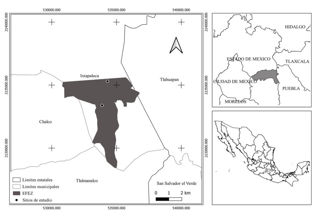
Figura 1. Localización del área de estudio Estación Forestal Experimental Zoquiapan (EFEZ).
En la región cercana a la zona de estudio se ubicaron 6 estaciones meteorológicas; sin embargo, los registros comprenden el periodo de 1961 al 2010, insuficientes para analizar el periodo de interés que se extiende hasta el 2023. Por tanto, se obtuvieron datos de precipitación y temperatura de la base de reanálisis NASA Prediction Of Worldwide Energy Resources (NASA POWER) (NASA POWER, 2023). Estos datos fueron sometidos a un análisis de correlación mediante el coeficiente de Pearson, con el propósito de compararlos con los registros de estaciones meteorológicas y confirmar la similitud y confiabilidad de la información proporcionada por NASA POWER (fig. 2). La vinculación de los eventos de sequía en el Estado de México con el índice de ancho de anillo total de P. montezumae se realizó con indicadores del Tzolkin Monitor de Sequía de Mesoamérica, desarrollado por el Instituto Mexicano de Tecnología del Agua (IMTA, 2020).
Para evaluar la influencia climática en el crecimiento radial de Pinus montezumae, se aplicó un análisis de función de respuesta, el cual consistió en obtener el coeficiente de correlación de Pearson, si los datos tienen una distribución normal en otro caso se obtuvo el coeficiente de Spearman entre las variables climáticas (precipitación total mensual, temperatura máxima, media y mínima) con los índices de las cronologías estandarizadas y residuales correspondientes al ancho de anillo total, madera temprana y madera tardía. Este análisis se hizo para el periodo 1982-2023 utilizando el coeficiente adecuado tras verificar la normalidad de los datos mediante la prueba de Shapiro-Wilk. Esto permitió determinar si el efecto de la variabilidad climática influye en el incremento radial del árbol.
Resultados
Se evaluó la relación entre la variabilidad climática y el crecimiento radial de Pinus montezumae en la Estación Forestal Experimental Zoquiapan. Para ello, se analizaron las correlaciones entre las cronologías estandarizadas y residuales del anillo total, madera temprana y tardía, con las variables climáticas de temperatura (promedio, máxima y mínima) y precipitación mensual. Los 26 árboles de Pinus montezumae presentaron diámetros que oscilaron entre 14 y 120 cm, y edades entre 34 y 123 años. De los 51 núcleos de crecimiento colectados, 45 (88%) fueron fechados con éxito; los restantes se excluyeron debido a la presencia de anillos falsos y ausentes.
Las cronologías del ancho de anillo total (AT), madera temprana (MTe) y madera tardía (MTa) abarcan un periodo común de 123 años, comprendido entre 1901 y 2023. La muestra más longeva data de 1901, mientras que la más reciente corresponde a 1981. El análisis de correlación entre las series de anillos de crecimiento, por segmentos de 50 años con traslapes de 25 años, indican que la calidad de fechado y la datación cruzada es correcta (p ˂ 0.01), superando la correlación mínima r = 0.3281 (tabla 1) establecida por Holmes (1983). Asimismo, los parámetros estadísticos de las series de anillos de crecimiento (tabla 1) respaldan el buen potencial dendroclimático de P. montezumae para estudios del crecimiento radial frente a la variabilidad climática.
Para identificar la función de respuesta del crecimiento radial a las variaciones climáticas, se generaron 2 cronologías: estándar y residual, a partir del índice de ancho de anillo total, madera temprana y madera tardía. Estas cronologías indican que el crecimiento promedio anual del ancho de anillo fue de 1.03 mm (tabla 2) y reflejan tendencias asociadas con periodos húmedos y de sequía. La cronología estándar fue la que determinó mejor la respuesta de P. montezumae a las fluctuaciones del clima, de acuerdo con la media del ancho de anillo (AT= 1.03, MTe = 1.0, MTa = 0.991), sensibilidad media (AT = 0.279, MTe = 0.138, MTa = 0.135), señal ruido (AT = 21.308, MTe = 15.353, MTa = 26.199). Las cronologías del índice de ancho de anillo total (IAA), madera temprana y madera tardía, tanto en su forma estándar (St) como residual (Rs), para P. montezumae comprenden un periodo de 123 años. Ambas series destacaron intervalos en los que el crecimiento radial fue superior a la media (fig. 3A), específicamente en los años 1901-1910, 1913-1917, 1942-1946, 1970-1972. En contraste, se observaron periodos de crecimiento por debajo del promedio durante 1923-1931, 1947-1950, 1961-1965, 1968-1976, 1998-2001 y 2021-2023.
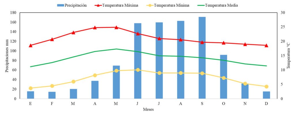
Figura 2. Climograma de la región EFEZ.
Las cronologías estándar y residual de la madera temprana presentaron una marcada variabilidad interanual en el crecimiento radial (fig. 3B). Los periodos con mayor desarrollo de madera temprana corresponden a los años 1901-1910, 1913-1916, 1931-1935, 1943-1947, 1978-1990 y 2002-2012. En contraste, se registró una menor formación de madera temprana durante los periodos 1923-1930, 1936-1942, 1961-1965, 1973-1977 y 1998-2001. Con respecto a las cronologías estándar y residual de la madera tardía también exhibieron una alta fluctuación interanual. Los periodos con mayor formación de madera tardía corresponden a los años 1903- 1904, 1907, 1909-1910, 1912, 1914-1915, 1917, 1923-1926, 1928-1930, 1935, 1937-1939, 1941- 1944, 1949-1951, 1954-1956, 1958-1962, 1969-1971, 1974-1977, 1983-1985, 1992 1995, 1996, 1998, 2003-2006, 2009-2010, 2014-2016 y 2018-2021 (fig. 3C).
Los eventos de sequía descritos por Domínguez (2016) y registrados en el Tzolkin Monitor de Sequía de Mesoamérica se asociaron a la cronología de ancho de anillo (fig. 4) y se observó que aquellos periodos de tiempo donde el crecimiento radial del árbol fue menor a la media anual corresponden a años con eventos de sequía, como son: la sequía de 1908 a 1910, las sequías de 1925, 1935, la de 1948 a 1954 que fue muy severa, 1957, 1960 a 1964, 1969, 1977. También se puede identificar que en el periodo de 1980 al 2023, el crecimiento radial estuvo influenciado por la presencia de sequías anuales de intensidad moderada, destacando el registro en la cronología de sequías severas en 2001, 2006-2012 y de 2018-2023.
Tabla 1
Estadísticos descriptivos de las series de anillos de crecimiento de P. montezumae.
| Parámetro estadístico | Anillo total | Madera temprana | Madera tardía |
| Intercorrelación entre series | 0.657 | 0.601 | 0.673 |
| Sensibilidad media | 0.281 | 0.324 | 0.278 |
| Desviación estándar | 0.875 | 0.758 | 0.223 |
| Autocorrelación de primer orden | 0.529 | 0.518 | 0.520 |
| Relación señal-ruido | 14.621 | 11.159 | 19.533 |
La función de respuesta del crecimiento radial de P. montezumae y la variabilidad del clima se analizó en el periodo común de 1981-2023. El análisis de correlación (coeficiente de Pearson), entre la cronología estandarizada de anillo total y la precipitación mensual, mostró correlaciones tanto positivas como negativas a lo largo del ciclo de crecimiento. La correlación entre el IAA estándar y precipitación mensual fue significativa en julio (r = 0.329, p = 0.033); mientras que, en el índice de madera temprana fue para septiembre del año anterior (r = -0.35, p = 0.049) y julio (r = 0.331, p = 0.032), para madera tardía fue en marzo (r = 0.373, p = 0.015) (fig. 5A). En los análisis de las cronologías residuales y la precipitación, la relación fue similar a la estándar, en el caso del índice de ancho de anillo fue significativa para septiembre del año anterior (r = -0.308, p = 0.046) y julio (r = 0.306, p = 0.048). Con respecto a la madera temprana, en septiembre del año anterior (r = -0.341, p = 0.027) y en madera tardía, en noviembre (r = 0.333, p = 0.031) y marzo (r = 0.373, p = 0.015) (fig. 5B).
La reciprocidad entre los índices de ancho de anillo AT, MTe, MTa y la temperatura (máxima, media y mínima) en el periodo común entre los años 1981 a 2023, reveló correlaciones negativas y positivas. Las asociaciones de los índices de ancho de anillo y la temperatura máxima, media y mínima con valores de coeficientes de correlación estadísticamente significativos (tabla 3), indican que las temperaturas máximas de septiembre y octubre del año anterior favorecieron el crecimiento del anillo total y la formación de madera temprana; sin embargo, en la cronología residual la temperatura máxima de enero afectó de forma negativa el desarrollo de madera tardía (fig. 6A, B).
Tabla 2
Estadísticas descriptivas de las cronologías estandarizada y residual de P. montezumae.
| Parámetros estadísticos | Cronologías | |||||
| Estándar | Residual | |||||
| Anillo total | Madera temprana | Madera tardía | Anillo total | Madera temprana | Madera tardía | |
| Ancho de anillo mm (media) | 1.03 | 1.00 | 0.991 | 0.992 | 0.987 | 0.991 |
| Sensibilidad media | 0.279 | 0.138 | 0.135 | 0.166 | 0.179 | 0.179 |
| Desviación estándar | 0.196 | 0.212 | 0.220 | 0.183 | 0.199 | 0.226 |
| Coeficiente de Gini | 0.110 | 0.120 | 0.124 | 0.104 | 0.113 | 0.124 |
| Autocorrelación de 1er orden | 0.125 | 0.092 | 0.196 | -0.162 | -0.180 | -0.100 |
| Relación señal-ruido | 21.308 | 15.353 | 26.199 | 27.802 | 20.144 | 34.543 |
| Señal expresada de la población (eps) | 0.950 | 0.934 | 0.958 | 0.965 | 0.953 | 0.972 |
Las correlaciones entre la temperatura mínima de octubre, noviembre, diciembre del año anterior con el índice de ancho de anillo de MTa y en diciembre con AT (fig. 6C, D), en la cronología estándar, fueron estadísticamente significativas; mientras que en la cronología residual solo fue significativa para noviembre; lo cual significa que las temperaturas mínimas de invierno favorecen la formación de madera tardía y puede deberse a que los árboles inician su etapa de letargo. Finalmente, la correlación entre la temperatura media de septiembre y octubre del año anterior fue estadísticamente significativa con el índice de madera tardía en la cronología estándar; en la cronología residual, únicamente la temperatura de octubre mostró una relación significativa (fig. 6E, F). Estos resultados reafirman la influencia de las temperaturas de otoño en la formación de madera tardía.
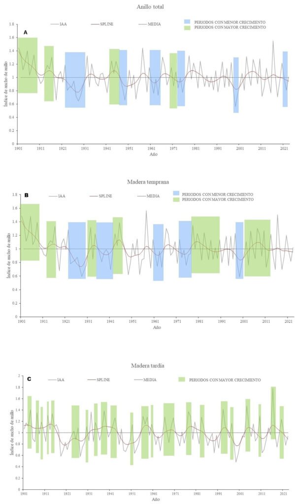
Figura 3. Cronología de índices de ancho de anillo de P. montezumae.
Discusión
Los resultados obtenidos aportan evidencia sobre la respuesta de Pinus montezumae a las condiciones ambientales, ya que se lograron identificar patrones de crecimiento mediante el fechado en 88% de las muestras. El porcentaje es considerado alto, puesto que en estudios dendrocronológicos es común excluir hasta 40% de las muestras debido a irregularidades en los anillos de crecimiento (Cerano-Paredes et al., 2014). La baja presencia de anillos falsos (menos de 5%) encontrada en P. montezumae coincide con lo registrado por Gutiérrez-García y Ricker (2019) y Villanueva-Díaz et al. (2016) para especies que habitan en la alta montaña.
Tabla 3
Coeficientes de correlación de Pearson de la relación entre índices de ancho de anillo y temperatura. * Mes del año anterior al inicio de la temporada de crecimiento.
| Temperatura | Mes | Índices de ancho de anillo de las Cronologías | |||||
| Estándar | Residual | ||||||
| Anillo total | Madera Temprana | Madera Tardía | Anillo total | Madera Temprana | Madera Tardía | ||
| Máxima | Septiembre* | r = 0.365 p = 0.017 | r = 0.353 p = 0.021 | – | r = 0.361 p = 0.018 | r = 0.356 p = 0.020 | – |
| Octubre* | r = 0.326 p = 0.034 | – | – | – | – | – | |
| Enero | – | – | – | – | – | r = -0.318 p = 0.039 | |
| Media | Septiembre* | – | – | r = 0.316 p = 0.041 | – | – | – |
| Octubre* | – | – | r = 0.362 p = 0.018 | – | – | r = 0.310 p = 0.045 | |
| Mínima | Octubre* | – | – | r = 0.323 p = 0.036 | – | – | – |
| Noviembre* | – | – | r = 0.365 p = 0.017 | – | – | r = 0.342 p = 0.026 | |
| Diciembre* | r = 0.318 p = 0.039 | – | r = 0.317 p = 0.040 | – | – | – |
Los valores de intercorrelación entre series fueron de 0.657 (anillo total), 0.601 (madera temprana) y 0.673 (madera tardía), similar a lo obtenido por Cortés-Cortés (2020) para P. montezumae en Coyuca de Catalán, Guerrero (r = 0.57), mayor al valor mínimo de 0 establecido por Holmes (1983), lo cual muestra que las intercorrelaciones de P. montezumae son estadísticamente significativas (p < 0.05). De acuerdo con Grissino-Mayer (2001), los valores de sensibilidad media del ancho total del anillo (0.281), madera temprana (0.324) y madera tardía (0.278) de P. montezumae representan una sensibilidad baja (0.135 – 0.179) e intermedia (0.279) en el ancho total del anillo. Estos valores son menores a los reportados para pináceas del norte de México, donde se obtuvieron valores mayores a 0.5 (Constante-García et al., 2010; Santillán-Hernández et al., 2016) y menores a los obtenidos para P. montezumae en Guerrero (0.31), según lo reportado por Cortés-Cortés (2020).
La autocorrelación de primer orden en los 3 índices de ancho de anillo muestra valores entre 0.092 y 0.196, lo cual es un criterio fundamental en estudios dendrocronológicos, debido a que una baja autocorrelación indica que el crecimiento radial no está significativamente influenciado por las condiciones climáticas del año anterior (Constante-García et al., 2010; Fritts, 1976). Estos resultados muestran que la especie es particularmente adecuada para estudios de reconstrucción climática porque permite registrar con mayor precisión las variaciones climáticas interanuales. De acuerdo con Briffa (1995), una cronología de sitio con un valor de señal expresada de la población (EPS) superior a 0.85, indica que el número de muestras es adecuado; en este estudio, se alcanzaron valores superiores, es decir, valores entre 0.934 y 0.972 para los 3 índices de crecimiento (AT, madera temprana y madera tardía), lo cual confirma la robustez de los datos analizados.
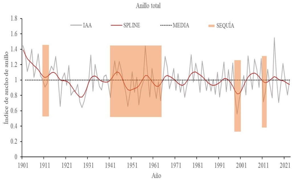
Figura 4. Vinculación de índice de ancho de anillo con eventos de sequía.
Los parámetros dendrocronológicos obtenidos para P. montezumae en este estudio, junto con los resultados reportados para la misma especie (Cortés-Cortés, 2020) y estudios de otras especies del centro del país, reconocidas por su buen potencial en este campo (Cerano-Paredes et al., 2014; Villanueva-Díaz et al., 2015, 2016), respaldan su utilidad en estudios dendrocronológicos. En consecuencia, se concluye que P. montezumae presenta un potencial dendrocronológico de moderado a alto, lo que la hace idónea para investigaciones orientadas a evaluar el impacto del clima y el cambio climático sobre el crecimiento radial. La relación entre el clima y el crecimiento radial indica que la disponibilidad de humedad, particularmente durante el invierno y la primavera, influye positivamente en el crecimiento de la especie. Este comportamiento coincide con un patrón que se presenta desde el sureste de los EUA hasta el centro de México, como lo han señalado diversos estudios (Allende et al., 2016; Cerano-Paredes et al., 2013; St. George et al., 2010; Villanueva-Díaz et al., 2016, 2017). Por lo tanto, las lluvias de baja intensidad, pero de larga duración junto con tasas moderadas de evaporación, permiten la retención de humedad en el suelo, favoreciendo el desarrollo durante los primeros meses de la temporada de crecimiento (Cerano-Paredes et al., 2009, 2011; Cleaveland et al., 2003; Constante-García et al., 2009; Díaz et al., 2002).
Por otra parte, las precipitaciones de verano y otoño del año de crecimiento actual presentan una variabilidad en su relación con las cronologías de P. montezumae; mientras que, los meses de otoño del año previo muestran correlaciones negativas y algunas estadísticamente significativas. Este patrón ha sido documentado también en investigaciones sobre otras especies del género Pinus (Cerano-Paredes et al., 2011, 2013; Chávez-Gándara et al., 2017; López-Hernández et al., 2018). Dicho comportamiento podría explicarse por la abundancia de lluvia durante estos periodos, que supera la capacidad de infiltración del suelo, provoca saturación de sus partículas, genera escurrimientos superficiales y limita así su disponibilidad para el desarrollo del árbol, así como por el hecho de que la mayor parte de los fotosintatos producidos en la temporada de lluvias se asignan al desarrollo de la copa, y se deja en segundo plano el incremento en el diámetro del tronco (Fritts, 1976). No obstante, esta lluvia es de gran importancia, pues parte de ella se almacena en el suelo y puede ser utilizada en la siguiente etapa de crecimiento (Meko et al., 1995).
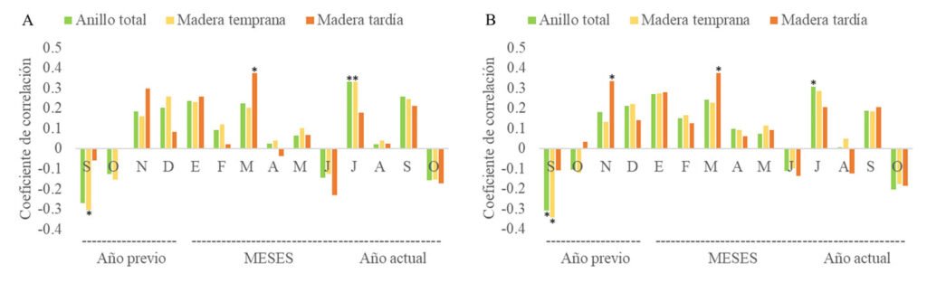
Figura 5. Coeficientes de correlación de precipitación e índices de ancho de anillo: A, estándar; B, residual.
El crecimiento de P. montezumae está principalmente influenciado y regulado por la disponibilidad de humedad durante el otoño del año previo y la primavera del año en curso. Al igual que otras especies estudiadas en investigaciones dendrocronológicas en el norte y centro de México, P. montezumae mostró una respuesta significativamente mayor a la precipitación que a la temperatura (Cerano-Paredes et al., 2013; Constante-García et al., 2010; Villanueva-Díaz et al., 2015, 2017). Los análisis de la temperatura máxima, mínima y media han identificado relaciones positivas entre estos factores y el crecimiento radial de los árboles en diversas partes del mundo, demostrando que la temperatura es un factor determinante en el desarrollo de los bosques, reflejándose en procesos clave, como la reactivación del cambium vascular, la diferenciación celular del xilema y la fotosíntesis, basándose en análisis de índices de ancho de anillo (Antonucci et al., 2017; Li et al., 2017, 2018; Zhu et al., 2016). Este estudio confirma la importancia de la temperatura en el crecimiento del P. montezumae debido a que se logra evidenciar, en algunos meses, el impacto de esta variable. De manera similar a lo observado en el estudio de P. montezumae realizado por Cortés-Cortés (2020), se identificaron principalmente relaciones positivas entre la temperatura máxima y la cronología estandarizada; además, en ambos estudios se observó una disminución en los valores estadísticamente significativos al correlacionarse con la cronología residual.
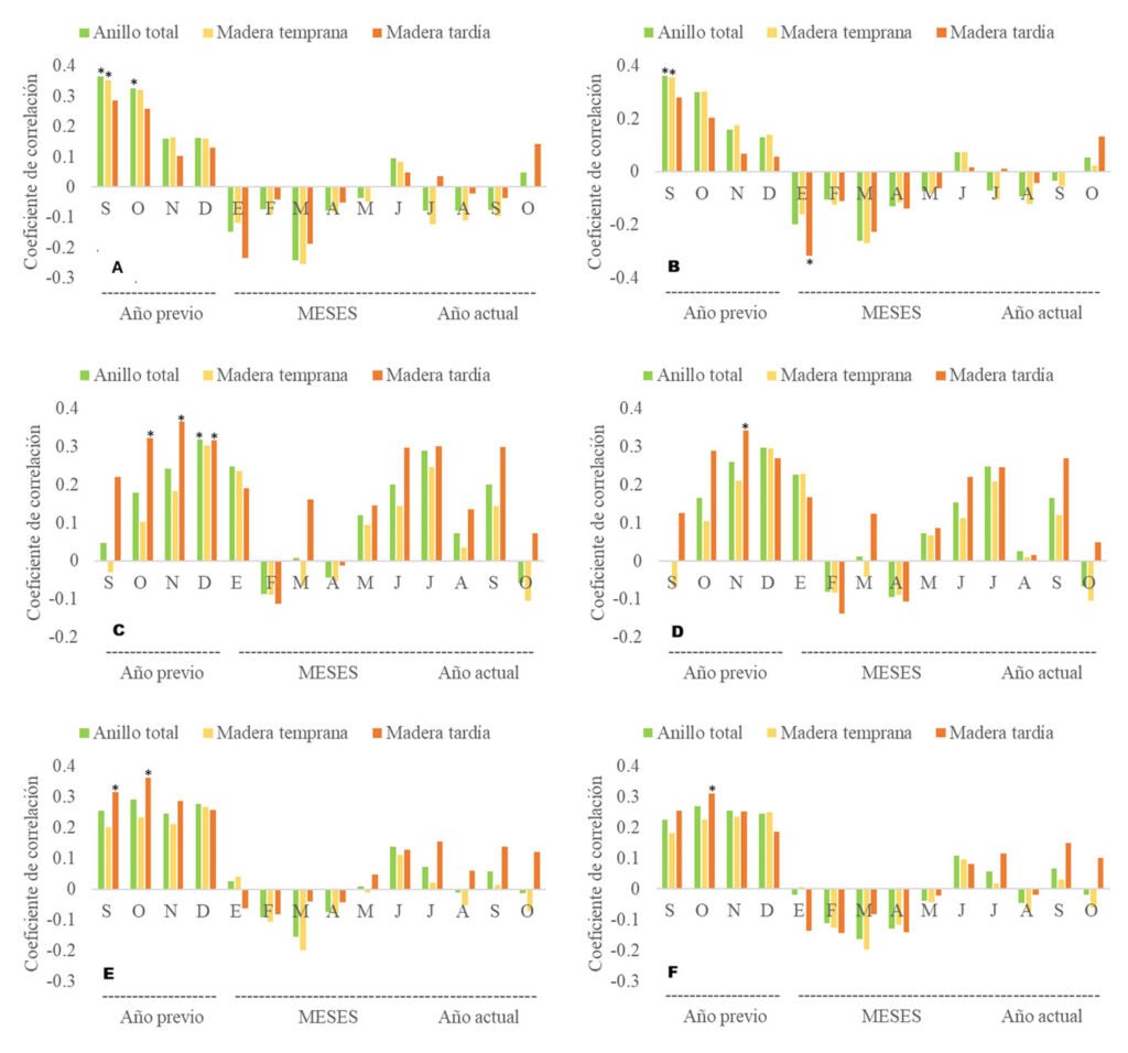
Figura 6. Coeficientes de correlación de temperatura e índices de ancho de anillo: A, relación temperatura máxima-cronología estándar; B, relación temperatura máxima-cronología residual; C, relación temperatura mínima – cronología estándar; D, relación temperatura mínima-cronología residual; E, relación temperatura media-cronología estándar; F, relación temperatura media-cronología residual.
En otros estudios de dendrocronología como el de Pinus hartwegii en el monte Tláloc ubicado también en la Faja Volcánica Transmexicana (Astudillo-Sánchez et al., 2017, 2019) y de Pinus oocarpa Schiede ex Schltdl del ejido Ojo de Agua, La Independencia en Chiapas, se han identificado correlaciones positivas entre las cronologías de ancho de anillo total y la temperatura máxima, éstas sugieren que la temperatura máxima incide en el crecimiento y desarrollo de madera tardía, tanto en la región central del país como en el sur, aunque se trate de especies con diferente rango de distribución (Astudillo-Sánchez et al., 2017, 2019; López-Hernández et al., 2018). La temperatura mínima mostró una influencia positiva en la mayoría de los meses analizados y destacó su efecto sobre la cronología de madera tardía, la cual presentó el mayor número de correlaciones positivas estadísticamente significativas. Estos hallazgos son consistentes con lo reportado en otros estudios dendrocronológicos realizados en México, que han encontrado correlaciones positivas significativas entre las temperaturas invernales y el crecimiento de diversas coníferas (Cerano-Paredes et al., 2012, 2014; Correa-Díaz et al., 2019; Chávez-Gándara et al., 2017; Huante et al., 1991; López-Hernández et al., 2018).
El crecimiento de las especies en respuesta a las temperaturas mínimas se debe, en gran medida, a que estas condiciones favorecen una menor evaporación del suelo y las plantas tienen una mayor disponibilidad de agua para el crecimiento (Cerano-Paredes et al., 2011; Chávez-Gándara et al., 2017). Con relación a la temperatura media, diversos estudios reportan que esta influye de manera negativa en el crecimiento radial (Cortés-Cortés et al., 2020; Manzanilla-Quiñones et al., 2020; Villanueva-Díaz et al., 2016). Sin embargo, en la presente investigación se identificó la presencia de correlaciones positivas, coincidiendo con lo reportado para otras especies de coníferas (Cerano-Paredes et al., 2014; Correa-Díaz et al., 2019). En la cronología residual se observaron correlaciones negativas de enero y mayo, un patrón que también se presentó al correlacionarse con la temperatura máxima. Este comportamiento puede atribuirse tanto al déficit hídrico como a que las temperaturas en la zona de estudio, en ciertos meses, se sitúan fuera del rango óptimo para la fotosíntesis en algunas coníferas, el cual oscila entre 15 y 25 °C, reduciéndose gradualmente en ambos extremos (Huxman et al., 2003; McCullough et al., 2017; Williams et al., 2013).
El crecimiento radial de P. montezumae responde a una interacción entre la temperatura y la precipitación. La disponibilidad de humedad en meses clave, como julio y marzo, junto con las temperaturas máximas en septiembre y octubre del año anterior, regulan conjuntamente la formación del crecimiento anual. Esto sugiere que el aumento en la temperatura puede favorecer el crecimiento solo cuando la precipitación es suficiente para mantener los procesos fisiológicos del árbol. Asimismo, las temperaturas mínimas durante el invierno parecen favorecer la formación de la madera tardía, lo que resalta la importancia de las condiciones térmicas en diferentes fases del ciclo anual. Los resultados coinciden con lo reportado por Harvey et al. (2020), quienes documentaron que el crecimiento radial en bosques templados está influenciado positivamente por inviernos cálidos, pero el efecto favorable del aumento temperatura puede verse limitado si no existe suficiente precipitación durante el verano. Por lo tanto, el impacto del cambio climático en el crecimiento de P. montezumae dependerá de la variación simultánea de la precipitación y la temperatura, por lo que es importante considerar ambas variables para predecir la respuesta de la especie en escenarios futuros.
Agradecimientos
A la Secretaría de Ciencia, Humanidades, Tecnología e Innovación (Secihti) por el otorgamiento de una beca para estudios de maestría al primer autor. A la División de Ciencias Forestales de la Universidad Autónoma Chapingo y al personal responsable de la Estación Forestal Experimental Zoquiapan, por el acceso y apoyo para la realización de esta investigación.
Referencias
Aber, J., Neilson, R. P., McNulty, S., Lenihan, J. M., Bachelet, D. y Drapek, R. J. (2001). Forest processes and global environmental change: predicting the effects of individual and multiple stressors. BioScience, 51, 735. https://doi.org/10.1641/0006-3568(2001)051
Allende, T. C., Mendoza, M. E., Pérez-Salicrup, D. R., Villanueva-Díaz, J. y Lara, A. (2016). Climatic responses of Pinus pseudostrobus and Abies religiosa in the Monarch Butterfly Biosphere Reserve, Central Mexico. Dendrochronologia, 38, 103–116. https://doi.org/10.1016/j.dendro.2016.04.002
Antonucci, S., Rossi, S., Deslauriers, A., Morin, H., Lombardi, F., Marchetti, M. et al. (2017). Large scale estimation of xylem phenology in black spruce through remote sensing. Agricultural and Forest Meteorology, 233, 92–100. https://doi.org/10.1016/j.agrformet.2016.11.011
Astudillo-Sánchez, C. C., Fowler, M. S., Villanueva-Díaz, J., Endara-Agramont, A. R. y Soria-Díaz, L. (2019). Recruitment and facilitation in Pinus hartwegii, a Mexican alpine treeline ecotone, with potential responses to climate warming. Trees, 33, 1087–1100. https://doi.org/10.1007/s00468-019-01844-3
Astudillo-Sánchez, C. C., Villanueva-Díaz, J., Endara-Agramont, A. R., Nava-Bernal, G. E. y Gómez-Albores, M. A. (2017). Climatic variability at the treeline of Monte Tlaloc, Mexico: a dendrochronological approach. Trees, 31, 441–453. https://doi.org/10.1007/s00468-016-1460-z
Benito, F. G. (2014). Archivos climáticos y paleohidrológicos. Introducción a datos proxy y su análisis. Madrid: CSIC- Museo Nacional de Ciencias Naturales.
Briffa, K. R. (1995). Interpreting high-resolution proxy climate data. The example of dendroclimatology. En H. von Storch y A. Navarra (Eds.), Analysis of climate variability, applications of statistical techniques (pp. 77–94). Berlin, Heidelberg: Springer. https://doi.org/10.1007/978-3-662-03167-4_5
Bunn, A. G. (2010). Statistical and visual crossdating in R using the dplR library. Dendrochronologia, 28, 251–258. https://doi.org/10.1016/j.dendro.2009.12.001
Bunn, A.G. (2008). A dendrochronology program library in R (dplR). Dendrochronologia, 26, 115–124. https://doi.org/10.1016/j.dendro.2008.01.002
Cassman, K. G. y Wood, S. (2005) Cultivated systems. En R. Hassan, R. Scholes y N. Ash (Eds.), Ecosystems and human well-being: current state and trends (pp. 745–794). Washington, DC; Millennium Ecosystem Assessment – Island Press.
Cerano-Paredes, J., Villanueva-Díaz J., Cervantes-Martínez, R., Vázquez-Selem, L., Trucios-Caciano, R. y Guerra-de la Cruz, V. (2014). Reconstrucción de precipitación invierno-primavera para el Parque Nacional Pico de Tancítaro, Michoacán. Investigaciones Geográficas, 83, 41–54. https://doi.org/10.14350/rig.35190
Cerano-Paredes, J., Villanueva-Díaz, J., Fulé, P. Z., Arreola-Ávila, J. G., Sánchez-Cohen, I. y Valdez-Cepeda, R. D. (2009). Reconstrucción de 350 años de precipitación para el suroeste de Chihuahua, México. Madera y Bosques, 15, 27–44. https://doi.org/10.21829/myb.2009.1521189
Cerano-Paredes, J., Villanueva-Díaz, J., Valdez-Cepeda, R. D., Méndez-González, J. y Constante-García, V. (2011). Sequías reconstruidas en los últimos 600 años para el noreste de México. Revista Mexicana de Ciencias Agrícolas, 2, 235–249. https://doi.org/10.21829/myb.2009.1521189
Cerano-Paredes, J., Rivera-González, M., Estrada-Ávalos, J., Trucios-Caciano, R. y Ríos-Saucedo, J. C. (2012). Análisis dendrocronológico de Pinus cooperi en Durango, México. Agrofaz, 12, 81–88.
Cerano-Paredes, J., Villanueva-Díaz, J., Cervantes-Martínez, R., Trucios-Caciano, R. y Guerrero-Soto, J. L. (2013). Reconstrucción de sequías fuertes en el Parque Nacional “Pico de Tancítaro”, Michoacán. Revista Chapingo, Serie Zonas Áridas, 2, 57–62. https://doi.org/10.5154/r.rchsza.2012.06.026
Chávez-Gándara, M. P., Cerano-Paredes, J., Nájera-Luna, J. A., Pereda-Breceda, V., Esquivel-Arriaga, G., Cervantes-Martínez, R. et al. (2017). Reconstrucción de la precipitación invierno-primavera con base en anillos de crecimiento de árboles para la región de San Dimas, Durango, México. Bosque, 38, 387–399. https://dx.doi.org/10.4067/S0717-92002017000200016
Cleaveland, M. K., Stahle, D. W., Therrell, M. D., Villanueva-Díaz, J. y Burns, B. T. (2003). Tree-ring reconstructed winter precipitation and tropical teleconnections in Durango, Mexico. Climatic Change, 59, 369–388. https://doi.org/10.1023/A:1024835630188
Conanp (Comisión Nacional de Áreas Naturales Protegidas). (2013). Programa de manejo del Parque Nacional Iztaccíhuatl-Popocatépetl. México. Recuperado el 15 agosto, 2024 de: https://conanp.gob.mx/conanp/dominios/iztapopo/documentos/programa_demanejo_izta_popo.pdf
Constante-García, V., Villanueva-Díaz, J., Cerano-Paredes, J., Cornejo-Oviedo, E. H. y Valencia-Manzo, S. (2009). Dendrocronología de Pinus cembroides Zucc. y reconstrucción de precipitación estacional para el Sureste de Coahuila. Ciencia Forestal en México, 34, 17–39.
Constante-García, V., Villanueva-Díaz, J., Cerano-Paredes, J. y Estrada-Ávalos, J. (2010). Parámetros para definir el potencial dendrocronológico. Folleto técnico número 19. Gómez Palacio, Durango: Instituto Nacional de Investigaciones Forestales, Agrícolas y Pecuarias.
Cook, E. R. y Kairiukstis, L. A. (1990) Methods of dendrochronology. Applications in the environmental sciences. Dordrecht, Holanda: International Institute for Applied Systems Analysis. Kluwer Academic Publishers.
Correa-Díaz, A., Silva, L. C. R., Horwath, W. R., Gómez-Guerrero, A., Vargas-Hernández, J., Villanueva-Díaz, J. et al. (2019). Linking remote sensing and dendrochronology to quantify climate-induced shifts in high-elevation forests over space and time. Journal of Geophysical Research: Biogeosciences, 124, 166–183. https://doi.org/10.1029/2018JG004687
Cortés-Cortés, O., Cornejo-Oviedo, E. H., Cerano-Paredes, J., Cervantes-Martínez, R., Flores-López, C. y Valencia-Manzo, S. (2020). Relationship between climate variability and radial growth of Pinus montezumae Lamb. in Coyuca de Catalán, Guerrero. Revista Chapingo, Serie Ciencias Forestales y del Ambiente, 27, 109–126. https://doi.org/10.5154/r.rchscfa.2020.03.012
Díaz, S. C., Therrell, M. D., Stahle, D. W. y Cleaveland, M. K. (2002). Chihuahua (México) winter-spring precipitation reconstructed from tree rings, 1647-1992. Climate Research, 22, 237–244. https://doi.org/10.3354/cr022237
Domínguez, J. (2016). Revisión histórica de las sequías en México: de la explicación divina a la incorporación de la ciencia. Tecnología y Ciencias del Agua, 7, 77–93.
Farjon, A., Pérez-de la Rosa, J. A. y Styles, B. T. (1997). Guía de campo de los pinos de México y América Central. Oxford, UK: The Royal Botanic Gardens, Kew/ Instituto Forestal de Oxford, Universidad de Oxford.
Fritts, H. C. (1976). Tree rings and climate. New York: Academic Press Inc.
Grissino-Mayer, H. D. (2001). Evaluating crossdating accuracy: a manual and tutorial for the computer program COFECHA. Tree-Ring Research, 57, 205–221.
Gutiérrez-García, G. y Ricker, M. (2019). Influencia del clima en el crecimiento radial en cuatro especies de coníferas en la sierra de San Antonio Peña Nevada (Nuevo León, México). Revista Mexicana de Biodiversidad, 90, e902676. https://doi.org/10.22201/ib.20078706e.2019.90.2676
Harvey, J. E., Smiljanić, M., Scharnweber, T., Buras, A., Cedro, A. Cruz-García, R. et al. (2020). Tree growth influenced by warming winter climate and summer moisture availability in northern temperate forests. Global Change Biology, 26, 2505–2518. https://doi.org/10.1111/gcb.14966
Holmes, R. L. (1983). Computer-assisted quality control in tree-ring dating and measurement. Tree-Ring Bulletin, 43, 69–78.
Howard, I. M., Stahle D. W., Torbenson, M. C. A. y Griffin, D. (2021). The summer precipitation response of latewood tree-ring chronologies in the southwestern United States. International Journal of Climatology, 41, 2913–2933. https://doi.org/10.1002/joc.6997
Huante, P., Rincón, E. y Swetnam, T. W. (1991). Dendrochronology of Abies religiosa in Michoacán, Mexico. Tree-Ring Bulletin, 51, 15–28.
Huxman, T. E., Turnipseed, A. A., Sparks, J. P., Harley, P. C. y Monson, R. K. (2003). Temperature as a control over ecosystem CO2 fluxes in a high-elevation, subalpine forest. Oecologia, 134, 537–546. https://doi.org/10.1007/s00442-002-1131-1
IMTA (Instituto Mexicano de la Tecnología del Agua). (2020). Tzolkin Monitor de Sequía de Mesoamérica. Instituto Mexicano de la Tecnología del Agua, Secretaría de Medio Ambiente Recursos Naturales, México. Recuperado el 18 agosto, 2024 de: http://galileo.imta.mx/Sequias/moseq/index.html
IPCC (Intergovernmental Panel on Climate Change). (2014). Climate Change 2014. Synthesis report. Contribution of working groups I, II and III to the fifth assessment report of the Intergovernmental Panel on Climate Change. Génova, Suiza: IPCC. Disponible: https://archive.ipcc.ch/pdf/assessment-report/ar5/syr/SYR_AR5_FINAL_full_wcover.pdf
IPCC (Intergovernmental Panel on Climate Change). (2021). Climate change 2021. A summary for all. IPCC. Disponible: https://www.ipcc.ch/report/ar6/wg1/downloads/outreach/IPCC_AR6_WGI_SummaryForAll.pdf
Li, M., Duan, J., Wang, L. y Zhu, H. (2018). Late summer temperature reconstruction based on tree-ring density for Sygera Mountain, southeastern Tibetan Plateau. Global and Planetary Change, 163, 10–17. https://doi.org/10.1016/j.gloplacha.2018.02.005
Li, X., Liang, E., Gricar, J., Rossi, S., Čufar, K. y Ellison, A. M. (2017). Critical minimum temperature limits xylogenesis and maintains treelines on the southeastern Tibetan Plateau. Science Bulletin, 62, 804–812. https://doi.org/10.1016/).scib.2017.04.025
López-Hernández, M. I., Cerano-Paredes, J., Valencia-Manzo, S., Cornejo-Oviedo, E. H., Villanueva-Díaz, J., Cervantes-Martínez, R. et al. (2018). Respuesta del crecimiento de Pinus oocarpa a variables climáticas en Chiapas, México. Biología Tropical, 66, 1580–1596. http://dx.doi.org/10.15517/rbt.v66i4.32663
Manzanilla-Quiñones, U., Aguirre-Calderón, O. A., Jiménez-Pérez, J. y Villanueva-Díaz, J. (2020). Sensibilidad climática en anchuras de anillos de crecimiento de Pinus hartwegii: una especie alpina mexicana con potencial dendroclimático. Revista Mexicana de Biodiversidad, 91, e913117. https://doi.org/10.22201/ib.20078706e.2020.91.3117
McCullough, I. M., Davis, F. W. y Williams, A. P. (2017). A range of possibilities: assessing geographic variation in climate sensitivity of ponderosa pine using tree rings. Forest Ecology and Management, 402, 223–233. https://doi.org/10.1016/j.foreco.2017.07.025
Meko, D., Stockton, C. W. y Boggess, W. R. (1995). The tree-ring record of severe sustained drought. JAWRA Journal of the American Water Resources Association, 31, 789–801. https://doi.org/10.1111/j.1752-1688.1995.tb03401.x
Meko, D. M. y Baisan, C. H. (2001). Pilot study of latewood-width of conifers as an indicator of variability of summer rainfall in the North American monsoon region. International Journal of Climatology, 21, 697–708. https://doi.org/10.1002/joc.646
NASA POWER. (2023). Prediction Of Worldwide Energy Resources. National Aeronautics and Space Administration (NASA), Washington D. C. Recuperado el 31 junio, 2024 de: https://power.larc.nasa.gov
Osorio-Osorio, J. A., Astudillo-Sánchez, C. C., Villanueva-Díaz, J., Soria-Díaz, L. y Vargas-Tristán, V. (2020). Reconstrucción histórica de la precipitación en la Reserva de la Biosfera El Cielo, México, mediante anillos de crecimiento en Taxodium mucronatum (Cupressaceae). Revista de Biología Tropical, 8, 818–832. https://doi.org/10.15517/rbt.v68i3.39624
Posit team (2024). RStudio. Integrated development environment for R. Posit Software, PBC, Boston, MA. https://www.posit.co/
Rzedowski, J. (2006). Vegetación de México. Comisión Nacional para el Conocimiento y Uso de la Biodiversidad. http://www.conabio.gob.mx/institucion/centrodoc/doctos/librosdigitales/VegetaciondeMexico/Portadaypaglegales.pdf
Santillán-Hernández, M., Cornejo-Oviedo, E. H., Villanueva-Díaz, J., Cerano-Paredes, J., Valencia-Manzo, S. y Capó-Arteaga, M. Á. (2016). Potencial dendroclimático de Pinus pinceana Gordon en la Sierra Madre Oriental. Madera y Bosques, 16, 17–30. https://doi.org/10.21829/myb.2010.1611177
Schweingruber, F. H. (1988). Tree rings: basics and applications of dendrochronology. Holanda: Dordrecht, Holanda: Kluwer Academic Publishers Group.
St. George, S., Meko, D. M. y Cook, E. R. (2010). The seasonality of precipitation signals embedded within the North American Drought Atlas. The Holocene, 20, 983–988. https://doi.org/10.1177/0959683610365937
Stokes, M. A. y Smiley, T. L. (1996). An introduction to tree-ring dating. Tucson: The University of Arizona Press.
Vaganov, E. A., Hughes, M. K. y Shashkin, A. V. (2006). Growth dynamics of conifer tree rings: images of past and future environments. Berlín, Heidelberg: Springer-Verlag.
Villanueva-Díaz, J., Rubio-Camacho, E. A., Chávez-Durán, A. A., Zavala-Aguirre, J. L., Cerano-Paredes, J. y Martínez-Sifuentes, A. R. (2017). Respuesta climática de Pinus oocarpa Schiede Ex Schetol en el Bosque La Primavera, Jalisco. Madera y Bosques, 24, 1–14. https://doi.org/10.21829/myb.2018.2411464
Villanueva-Díaz, J., Cerano-Paredes, J., Vázquez-Selem, L., Stahle, D. W., Fulé, P. Z., Yocom, L. L. et al. (2015). Red dendrocronológica del pino de altura (Pinus hartwegii Lindl.) para estudios dendroclimáticos en el noreste y centro de México. Investigaciones Geográficas, 86, 5–14. https://doi.org/10.14350/rig.42003
Villanueva-Díaz, J., Vázquez-Selem, L., Gómez-Guerrero, A., Cerano-Paredes, J., Aguirre-González, N. A. y Franco-Ramos, O. (2016). Potencial dendrocronológico de Juniperus monticola Martínez en el Monte Tláloc, México. Revista Fitotecnia Mexicana, 39, 175–185. https://doi.org/10.35196/rfm.2016.2.175-185
Williams, A. P., Allen, C. D., Macalady, A. K., Griffin, D., Woodhouse, C. A., Meko, D. M. et al. (2013). Temperature as a potent driver of regional forest drought stress and tree mortality. Nature Climate Change, 3, 292–297. https://doi.org/10.1038/nclimate1693
Zhu, L., Zhang, Y., Li. Z., Guo, B. y Wang, X. (2016). A 368-year maximum temperature reconstruction based on tree-ring data in the northwestern Sichuan Plateau (NWSP), China. Climate of the Past, 12, 1485–1498. https://doi.org/10.5194/cp-12-1485-2016

Population density and sexual maturity of Ambystoma lermaense, an endangered species in central Mexico
Densidad poblacional y madurez sexual de Ambystoma lermaense, una especie amenazada en el centro de México
Gerardo Legorreta-Balbuena a, Carlos Omar Becerra-Soria b, Susana Hernández-Monasterio b, Gabriela Parra-Olea b, *
a Universidad Nacional Autónoma de México, Instituto de Investigaciones Biomédicas, Laboratorio de Biología Integrativa, Tercer Circuito s/n, Ciudad Universitaria, Col. Copilco Universidad, 04510 Ciudad de México, Mexico
b Universidad Nacional Autónoma de México, Instituto de Biología, Departamento de Zoología, Tercer Circuito s/n, Ciudad Universitaria, Col. Copilco Universidad, 04510 Ciudad de México, Mexico
*Corresponding author: gparra@ib.unam.mx (G. Parra-Olea)
Received: 21 January 2025; accepted: 14 November 2025
Abstract
Ambystoma lermaense, an endangered salamander species endemic to central Mexico, faces significant threats from habitat degradation, pollution, and human activities. This study evaluates the population density, structure, and sexual maturity of A. lermaense in Capilla Vieja, Estado de México, over 3 time periods: 2009, 2010, and 2020. Using visual encounter surveys along a 730-m stream transect, we recorded population densities of 0.021 individuals/m² in 2009, 0.070 individuals/m² in 2010, and 0.075 individuals/m² in 2020, reflecting relative stability despite anthropogenic pressures. Juveniles accounted for 87% of the population, with sexual maturity observed at a snout-vent length of 60 mm, supported by histological evidence of vitellogenic oocytes in females and mature sperm in males. Our study provides important insights into the population dynamics and sexual maturity of A. lermaense in the sampling locality, where this species had not been previously studied.
Keywords: Ambystomatidae; Population structure; Paedomorphosis; Vitellogenic oocytes; Mature sperm; Decline
Resumen
Ambystoma lermaense, una especie de salamandra en peligro de extinción endémica del centro de México, enfrenta amenazas significativas debido a la degradación del hábitat, la contaminación y las actividades humanas. Este estudio evalúa la densidad poblacional, estructura y madurez sexual de A. lermaense en Capilla Vieja, Estado de México, durante 3 períodos: 2009, 2010 y 2020. Utilizando muestreos visuales a lo largo de un transecto de 730 m en un arroyo, registramos densidades poblacionales de 0.021 individuos/m² en 2009, 0.070 individuos/m² en 2010 y 0.075 individuos/m² en 2020, lo cual refleja una estabilidad relativa a pesar de las presiones antropogénicas. Los juveniles representaron 87% de la población y se observó madurez sexual a un tamaño de 60 mm de longitud hocico-cloaca, sustentado por evidencia histológica de ovocitos vitelogénicos en hembras y espermatozoides maduros en machos. Nuestro estudio proporciona información importante sobre la dinámica poblacional y la madurez sexual de A. lermaense en la localidad de muestreo, donde esta especie no había sido estudiada previamente.
Palabras clave: Ambystomatidae; Estructura poblacional; Paedomorfosis; Ovocitos vitelogénicos; Espermatozoides maduros; Declive
Introduction
Amphibians worldwide are experiencing unprecedented declines, driven by a combination of habitat loss, pollution, climate change, invasive species, and disease (Grant et al., 2016; Stuart et al., 2004). These declines are particularly concerning for high-altitude amphibians, which often have restricted ranges and specialized habitat requirements (Green, 2003; Pounds, 2001; Stuart et al., 2004). As indicators of ecosystem health, amphibians play critical roles in maintaining ecological balance, yet they are disproportionately affected by anthropogenic pressures (Blaustein & Wake, 1990). Among these, Ambystoma lermaense, an endangered salamander species endemic to central Mexico, exemplifies the challenges faced by amphibians in fragmented and degraded habitats (IUCN SSC Amphibian Specialist Group, 2015).
Ambystoma lermaense, inhabits high-altitude streams at elevations ranging from 2,500 to 3,000 m asl (IUCN SSC Amphibian Specialist Group, 2015). This facultatively paedomorphic species is found in aquatic habitats such as lakes, ponds, marshes, and occasionally streams (Everson et al., 2021; IUCN SSC Amphibian Specialist Group, 2015), which are increasingly impacted by human activities (Reilly & Brandon, 1994). Agricultural expansion, livestock grazing, pollution, and urban development threaten the quality and connectivity of these aquatic habitats (Egea-Serrano et al., 2012; Robles-Mendoza et al., 2009). These pressures, combined with seasonal hydrological fluctuations and climate variability, pose significant risks to the long-term viability of A. lermaense populations (Dirzo et al., 2022; Huacuz-Elías, 2003).
Understanding population dynamics is a cornerstone of effective conservation planning. Accurate data on population density, structure, and trends are essential for identifying populations at risk and prioritizing interventions (Pechmann et al., 1991). Previous studies on species of the genus Ambystoma have revealed a wide spectrum of population densities, ranging from critically low levels in urbanized environments to exceptionally high densities in protected areas. For instance, the Mexican axolotl (A. mexicanum) exhibits densities as low as 0.001 individuals per square meter in the urban canals of Xochimilco (Contreras et al., 2009), while A. rivulare densities reach 2.3 individuals per square meter in the protected natural area Reserva de la Biósfera Mariposa Monarca (Huacuz-Elías, 2003). These disparities underscore the profound impact of habitat quality and protection on amphibian populations.
Despite its resilience in suboptimal conditions, A. lermaense remains highly vulnerable to habitat degradation and fragmentation (Jacinto-Maldonado et al., 2023). In the Capilla Vieja region of Estado de México, semi-intensive livestock activities and seasonal stream drying compound the challenges faced by this species (previously recognized in this locality as A. granulosum; Everson et al., 2021). As part of a natural protected area, Capilla Vieja offers a unique opportunity to study how A. lermaense populations persist in a landscape that combines elements of protection and human impact. The site’s connectivity to a broader watercourse system also provides insights into the role of habitat corridors in sustaining population viability.
This study examines the population density, structure, and sexual maturity of A. lermaense in Capilla Vieja over 3 time periods: 2009, 2010, and 2020. By situating these findings within the broader context of Ambystoma conservation, we aim to draw comparisons with other populations and species to better understand the factors driving population trends. The research also highlights the critical role of protected areas and localized conservation actions in addressing the multifaceted threats to amphibians. This work contributes to the growing body of knowledge needed to inform strategies for safeguarding A. lermaense and other endangered amphibians in Mexico’s diverse ecosystems.
Materials and methods
The study was conducted in a section of a stream located in Capilla Vieja, municipality of Amanalco de Becerra, Estado de México, at coordinates 19º13’22” N, 99º59’12” W, with an elevation ranging from 2,790 to 2,870 m asl (Fig. 1). The predominant vegetation in this area is pine-oak-fir forest. The climate is temperate subhumid, with summer rains, an average annual temperature of 12 °C, and temperature extremes ranging from 0.5 °C to 29.7 °C (Rentería et al., 2005). Capilla Vieja is part of the sustainable ecosystem management subzone for agricultural areas within the Natural Protected Area known as Área de Protección de Recursos Naturales de las Cuencas de los Ríos Valle de Bravo, Malacatepec, Tilostoc y Temascaltepec (Semarnat, 2018).
The study stream crosses an extensive grassland plain that is used for semi-intensive livestock activities, including sheep, cattle, and horses. The stream during the rainy season features shallow areas with nearly stagnant water. In certain sections, the bottom is extremely soft, with mud depths ranging from 15 to 25 cm and exceeding 50 cm in some points. The stream width varies between 2 and 5 m, expanding during the rainy season and shrinking or disappearing during the dry season. This stream is part of a connected watercourse system that flows in a northeast-southwest direction, contributing to the water supply of the Capilla Vieja lagoon (Comisión Nacional de Áreas Naturales Protegidas, 2018).
Samplings were conducted once a month from July to October during 3 periods corresponding to the years 2009, 2010 and 2020. Each month, a 730 m transect with a width of 3 m along the stream was surveyed (starting coordinates: 19°13’10.81” N, 99°59’4.95” W; ending coordinates: 19°13’3.73” N, 99°59’15.13” W). Sampling was carried out using the visual encounter survey method between 09:00 and 14:00 hours (Heyer et al., 1994; Lips et al., 1999), recording the total number of individuals. Each individual was captured using hand nets and placed in 20-liter plastic containers filled with water from the stream.
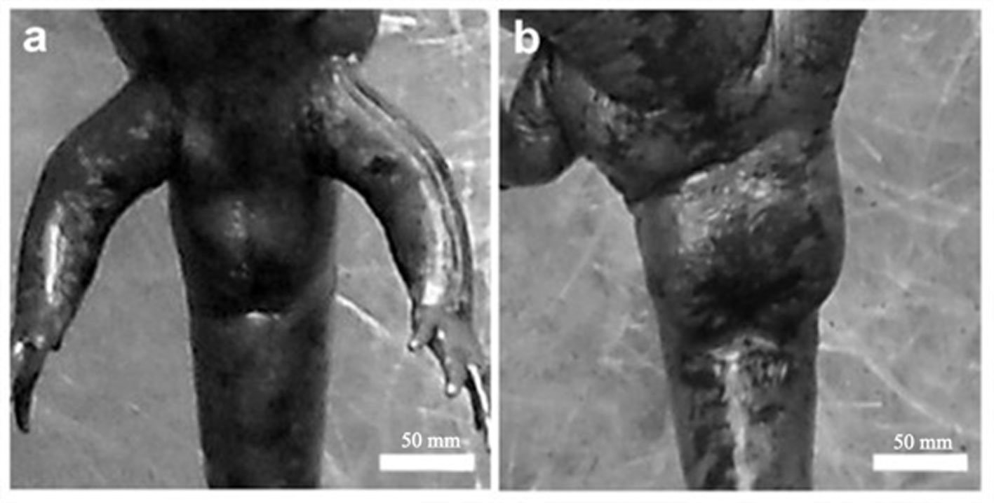
Morphometric measurements were recorded for each specimen: snout-vent length (SVL), total length (TL), and weight (W). Individuals were classified into 2 categories: adult metamorphic (males and females) and larvae (juveniles), a category that included individuals with gills for whose sex could not be determined. Population density was calculated by dividing the total number of individuals (N) by the sampled area of the stream (N/m²) (Williams et al., 2002), and it was estimated for each sampling period. Males and females were identified based on the size and shape of the cloaca (Aguilar-Miguel et al., 2009; Taylor, 1940). In females, the cloaca is flat and smaller (Fig. 2a), whereas in males it is enlarged due to high glandular activity (Fig. 2b).
To estimate the size at sexual maturity, a sample of 52 individuals was collected from random points along the stream during the 2009 and 2010 sampling periods. The sample included individuals ranging in size from 50 to 115 mm in SVL. An ANOVA was used to assess the relationship between body size and sexual maturity.
To euthanize the specimens, they were anesthetized using a 0.1% solution of MS-222 (tricaine methanesulfonate) for 20 min (Mitchell, 2009; Rubio-Limonta & Silveira-Coffigny, 2009). A longitudinal ventral incision was made to expose the ovaries and testes. The gonads were fixed in 4% paraformaldehyde for 24 h at 4 °C. Standard histological techniques for light microscopy were applied: dehydration in graded alcohols, clearing with xylene, embedding in paraplast, sectioning at 5 µm, and Hematoxylin-Eosin staining (Aguilar-Miguel et al., 2009). Digital images of spermatogenesis and oogenesis stages were captured using a Nikon Coolpix 4300 (4 MP) digital camera mounted on a Nikon Optiphot-2 upright microscope and calibrated with ImageJ software.
Results
A total of 366 individuals were recorded across the 2,190 m² of the sampled stream during the 3 periods (Table 1). The period with the lowest abundance was 2009, with 46 individuals, while the highest was 2020, with 165 individuals. The population density of A. lermaense increased over the sampling periods. In 2009, the density was 0.021 ind/m², in 2010, it increased to 0.070 ind/m², and finally, in 2020, it reached 0.075 ind/m².
Table 1
Total number of individuals recorded during the sampling periods.
| Period | July | August | September | October | Total |
| 2009 | 4 | 23 | 14 | 5 | 46 |
| 2010 | 4 | 56 | 70 | 25 | 155 |
| 2020 | 7 | 130 | 23 | 5 | 165 |
| Total | 15 | 209 | 107 | 35 | 366 |
Population structure. Of the total number of individuals found across the 3 periods, 87% were juveniles, 6% were metamorphic females, and 7% were metamorphic males. Throughout the 3 sampling periods, the months with the highest number of larvae were August and September, for metamorphic females, July and September, and for metamorphic males, August and September (Fig. 3).
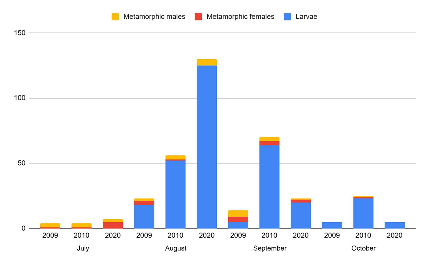
Table 2
Morphometric data (average, minimum, and maximum) of individuals analyzed histologically to determine sexual maturity. SVL = Snout-vent length, TL = total length (mm), and weight (g).
| Category | Metamorphic females | Metamorphic males | Larvae |
| Avg. SVL | 81.4 | 90.8 | 62.5 |
| Min. SVL | 60 | 60 | 50 |
| Max. SVL | 100 | 115 | 85 |
| Avg. TL | 156.1 | 167.9 | 114.6 |
| Min. TL | 130 | 110 | 85 |
| Max. TL | 180 | 220 | 155 |
| Avg. weight | 23.53 | 20.13 | 9.57 |
| Min. weight | 10 | 8 | 4 |
| Max. weight | 42 | 36 | 20 |
| Gonadal development (Yes/No) | Yes | Yes | No |
| Number of individuals | 14 | 24 | 14 |
Sexual maturity. Of the 52 dissected individuals, 24 were males, 14 females and 14 larvae. Males had an SVL ranging from 60 to 115 mm, females from 60 to 100 mm, and larvae from 50 to 85 mm (Table 2). According to the ANOVA, a significant association was found between size and the different age categories (p < 0.05). Through histological analysis, 38 individuals exhibited sexual development (Table 2). We determined that sexual maturity occurs at an SVL of 60 mm, as vitellogenic oocytes in females and mature sperm in males were observed at this size (Fig. 4).
Discussion
Our study on Ambystoma lermaense in Capilla Vieja provides critical insights into its population dynamics, sexual maturity, and conservation status. By situating these findings within a broader ecological and conservation context, we can deepen our understanding of the factors influencing the persistence of this species and its relatives. The gradual increase in population density from 0.021 individuals/m² in 2009 to 0.075 individuals/m² in 2020 is a positive indicator of stability. However, these densities remain substantially lower than those reported by Huacuz (2003) in the Reserva de la Biosfera Mariposa Monarca (2.3 individuals/m²). This stark contrast underscores the influence of habitat quality and protection on population viability. The Capilla Vieja site, despite being part of a protected natural area, is exposed to semi-intensive livestock activities and seasonal hydrological fluctuations, both of which could limit carrying capacity for A. lermaense.
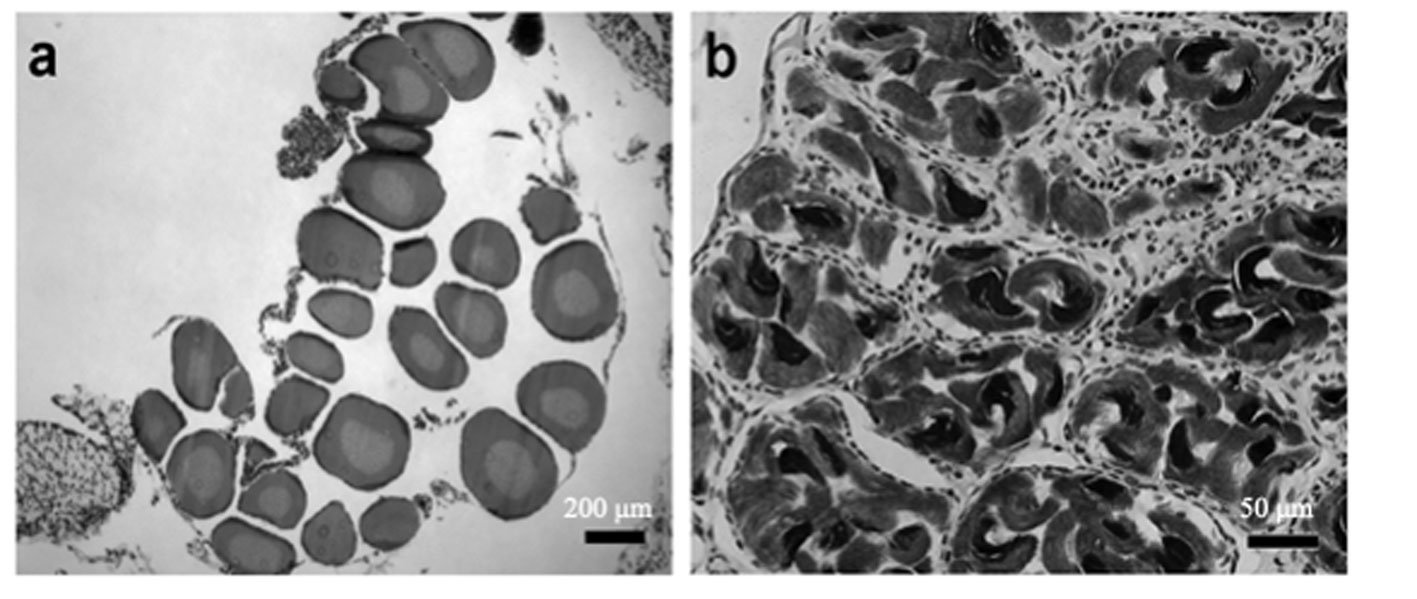
Examining densities and threats across 3 Ambystoma species provides valuable comparative insights: Ambystoma mexicanum, critically low densities in Xochimilco lake (0.001 individuals/m²) highlight severe impacts from urbanization and habitat degradation (Contreras et al., 2009). Ambystoma altamirani, densities ranging from 0.016 to 0.027 individuals/m² in trout-free streams in Estado de México suggest that invasive species exacerbate population declines (Lemos-Espinal et al., 1999). Ambystoma ordinarium, densities of 0.030-0.050 individuals/m² in Michoacán State highlight the challenges posed by deforestation and agricultural expansion (Aguilar-Miguel, 2005). These comparisons reinforce the role of protected areas in supporting higher population densities and the importance of mitigating threats in unprotected habitats.
The discovery that sexual maturity in A. lermaense occurs at a SVL of 60 mm aligns with findings for other facultatively paedomorphic Ambystoma species. Paedomorphosis, the retention of larval traits in adults, allows these salamanders to reproduce in aquatic habitats, potentially enhancing resilience in fragmented or fluctuating environments. However, the high proportion of juveniles (87%) in Capilla Vieja suggests a reliance on consistent recruitment, which could be disrupted by environmental changes.
The Capilla Vieja site is part of a connected watercourse system, but its fragmentation due to agricultural activities and seasonal stream drying limits habitat availability. Maintaining connectivity between breeding and non-breeding habitats is critical for sustaining gene flow and reducing local extinction risks. Lessons from the Reserva de la Biosfera Mariposa Monarca, where robust habitat connectivity supports high densities of this species, should guide management strategies for fragmented landscapes.
High-altitude amphibians like A. lermaense are particularly vulnerable to climate change. Rising temperatures and altered precipitation patterns could shrink suitable habitat ranges and exacerbate seasonal drying of streams. Proactive measures, such as restoring vegetation cover and monitoring hydrological changes, are necessary to mitigate these effects. While protected areas like the Reserva de la Biosfera Mariposa Monarca demonstrate the effectiveness of large-scale conservation, localized efforts are equally vital. Capilla Vieja’s inclusion in a protected area offers an opportunity to implement targeted interventions, such as: enhancing water quality through pollution control; reducing the impact of livestock on stream habitats; and introducing community-based conservation programs to engage local stakeholders.
The findings on A. lermaense reflect broader trends in amphibian conservation. Amphibians worldwide face similar threats of habitat degradation, invasive species, and climate change. This study contributes to the growing body of evidence that localized conservation actions, combined with broader protections, can stabilize and even enhance populations of threatened species. Future studies could explore: genetic diversity, assessing genetic variation in A. lermaense populations to evaluate the effects of fragmentation on genetic health. Behavioral ecology, investigating breeding behavior, dispersal patterns, and predator-prey dynamics to inform conservation strategies. Impact of invasive species, examining whether invasive species, such as trout, are encroaching on nearby A. lermaense habitats.
The relatively stable population density of Ambystoma lermaense in Capilla Vieja reflects its resilience but highlights the challenges posed by habitat degradation and fragmentation. Comparisons with other Ambystoma species and populations in protected areas underscore the importance of habitat quality and connectivity. To ensure the long-term survival of A. lermaense and its relatives, conservation efforts must integrate habitat restoration, community engagement, and climate adaptation strategies. As amphibians are critical indicators of ecosystem health, their protection benefits biodiversity and ecological integrity on a broader scale.
Acknowledgments
We gratefully acknowledge Conahcyt for the scholarship awarded to GL-B during his PhD studies in Biological Sciences at UNAM (2009–2011; registration number 161331). We also thank Gabriel Gutiérrez-Ospina for funding provided through GlaxoSmithKline, as well as the annual budget allocated to the Integrative Biology Laboratory by the Administrative Secretariat of the Institute of Biomedical Research, UNAM, which partially supported this project. Additional support was provided by DGAPA-UNAM (PAPIIT-UNAM, IN208024) and Secihti(CBF-2025-G-418) to GP-O. We are grateful to Fernando Arana Magallón, coordinator of the Biological and Aquaculture Research Center of Cuemanco (CIBAC-UAM-X), for his assistance with fieldwork, laboratory work, and specimen collection. We also thank Miguel Tapia-Rodríguez, head of the Microscopy Unit at IIB-UNAM, for his support in figure design. We acknowledge Semarnat for the permits granted for this study (Nos. SGPA/DGVS/00417/09, SGPA/DGVS/02729/10, and SGPA/DGVS/03197/20). Finally, we thank the two anonymous reviewers and the section editor for their valuable comments, which improved the manuscript.
References
Aguilar-Miguel, X. (2005). Ambystoma ordinarium. Algunas especies de anfibios y reptiles contenidos en el Proyecto de Norma Oficial Mexicana PROY-NOM-059-ECOL-2000. Facultad de Ciencias, Centro de Investigación en Recursos Bióticos, Universidad Autónoma del Estado de México.
Aguilar-Miguel, X., Legorreta-Balbuena, G., & Casas-Andreu, G. (2009). Reproducción ex situ en Ambystoma granulosum y Ambystoma lermaense (Amphibia: Ambystomatidae). Acta Zoológica Mexicana, 25, 443–454. https://doi.org/10.21829/azm.2009.253652
Blaustein, A. R., & Wake, D. B. (1990). Declining amphibian populations: a global phenomenon? Trends in Ecology & Evolution, 5, 203–204. https://doi.org/10.1016/0169-5347(90)90129-2
Semarnat (Secretaría de Medio Ambiente y Recursos Naturales). (2018). Acuerdo por el que se da a conocer el resumen del Programa de Manejo del Área Natural Protegida con la categoría de área de protección de recursos naturales cuencas de los ríos Valle de Bravo, Malacatepec, Tilostoc y Temascaltepec, Estado de México. Diario Oficial de la Federación. Normateca Ambiental. https://normatecambiental.org/2018/12/05/acuerdo-por-el-que-se-da-a-conocer-el-programa-de-manejo-del-area-natural-protegida-de-cuencas-de-los-rios-valle-de-bravo-malacatepec-tilostoc-y-temascaltepec-estado-de-mexico/
Contreras, V., Martínez-Meyer, E., Valiente, E., & Zambrano, L. (2009). Recent decline and potential distribution in the last known wild populations of the critically endangered Mexican Axolotl. Biological Conservation, 142, 2881–2885. https://doi.org/10.1016/j.biocon.2009.07.008
Dirzo, R., Ceballos, G., & Ehrlich, P. R. (2022). Circling the drain: the extinction crisis and the future of humanity. Philosophical Transactions of the Royal Society B, 377, 20210378. https://doi.org/10.1098/rstb.2021.0378
Egea-Serrano, A., Relyea, R. A., Tejedo, M., & Torralva, M. (2012). Understanding the impact of chemicals on amphibians: a meta-analytic review. Ecology and Evolution, 2, 1382–1397. https://doi.org/10.1002/ece3.249
Everson, K. M., Gray, L. N., Jones, A. G., Lawrence, N. M., Foley, M. E., Sovacool, K. L. et al. (2021). Geography is more important than life history in the recent diversification of the tiger salamander complex. Proceedings of the National Academy of Sciences, 118, e2014719118. https://doi.org/10.1073/pnas.2014719118
Grant, E. H. C., Miller, D. A. W., Schmidt, B. R., Adams, M. J., Amburgey, S. M., Chambert, T. et al. (2016). Quantitative evidence for the effects of multiple drivers on continental-scale amphibian declines. Scientific Reports, 6, 25625. https://doi.org/10.1038/srep25625
Green, D. M. (2003). The ecology of extinction: population fluctuation and decline in amphibians. Biological Conservation, 111, 331–343. https://doi.org/10.1016/S0006-3207(02)00302-6
Heyer, W. R., Donnelly, M. A., McDiarmid, R. W., Hayek, A. C., & Foster, M. S. (1994). Measuring and monitoring biological diversity: standard methods for amphibians. Washington D.C.: Smithsonian Institution Press.
Huacuz-Elías, D. C. (2003). Estado de conservación de Ambystoma lermaense Taylor, (1940) en el Santuario Sierra Chincua de la Reserva de la Biosfera “Mariposa Monarca”. Revista de la Facultad de Biología de la UMSNH, 5, 51–63.
IUCN SSC Amphibian Specialist Group. (2015). Ambystoma lermaense (errata version published in 2020). The IUCN Red List of Threatened Species 2015: e.T1093A176771946. https://dx.doi.org/10.2305/IUCN.UK.2015-4.RLTS.T1093A176771946.en
Jacinto-Maldonado, M., González-Salazar, C., Basanta, M. D., García-Peña, G. E., Saucedo, B., Lesbarrères, D. et al. (2023). Water pollution increases the risk of chytridiomycosis in Mexican amphibians. EcoHealth, 20, 74–83. https://doi.org/10.1007/s10393-023-01631-0
Lemos-Espinal, J. A., Smith, G. R., Ballinger, R. E., & Ramírez-Bautista, A. (1999). Status of protected endemic salamanders (Ambystoma: Ambystomatidae: Caudata) in the transvolcanic belt of Mexico. British Herpetological Society Bulletin, 68, 1–4.
Lips, K. R., Reaser., J. K., & Young, B. (1999). Monitoreo de anfibios en América Latina: manual de protocolos. Herpetological Circular No. 30. https://amphibiaweb.org/resources/Anfibios.pdf
Mitchell, M. A. (2009). Anesthetic considerations for amphibians. Journal of Exotic Pet Medicine, 18, 40–49. https://doi.org/10.1053/j.jepm.2008.11.006
Pechmann, J. H., Scott, D. E., Semlitsch, R. D., Caldwell, J. P., Vitt, L. J., & Gibbons, J. W. (1991). Declining amphibian populations: the problem of separating human impacts from natural fluctuations. Science, 253, 892–895. https://doi.org/10.1126/science.253.5022.892
Pounds, J. (2001). Climate and amphibian declines. Nature, 410, 639–640. https://doi.org/10.1038/35070683
Reilly, S. M., & Brandon, R. A. (1994). Partial paedomorphosis in the Mexican stream ambystomatids and the taxonomic status of the genus Rhyacosiredon Dunn. Copeia, 1994, 656–662. https://doi.org/10.2307/1447181
Rentería, G., Cota, R. G., & Ortega, E. (2005). Descripción del medio natural de la cuenca del Valle de Bravo, Estado de México. Jiutepec, Morelos: Instituto Mexicano de Tecnología del Agua.
Robles-Mendoza, C., García-Basilio, C., Cram-Heydrich, S., Hernández-Quiroz, M., & Vanegas-Pérez, C. (2009). Organophosphorus pesticides effect on early stages of the axolotl Ambystoma mexicanum (Amphibia: Caudata). Chemosphere, 74, 703–710. https://doi.org/10.1016/j.chemosphere.2008.09.087
Rubio-Limonta, M., & Silveira-Coffigny, R. (2009). Bienestar de los animales acuáticos, con fines de control sanitario. REDVET. Revista Electrónica de Veterinaria, 10. https://www.redalyc.org/pdf/636/63617143009.pdf
Stuart, S. N., Chanson, J. S., Cox, N. A., Young, B. E., Rodrigues, A. S., Fischman, D. L. et al. (2004). Status and trends of amphibian declines and extinctions worldwide. Science, 306, 1783–1786. https://doi.org/10.1126/science.1103538
Taylor, E. H. (1940). A new Rhyacosiredon (Caudata) from western México. Herpetologica, 1, 171–176.
Williams, L. R., Crosswhite, D. L., & William, M. G. (2002). Short-term effect of riparian disturbance on Desmog-
nathus brimleyorum (Plethodontidae) at natural spring in Oklahoma, U.S.A. The Southwestern Naturalist, 47,
611–613. https://doi.org/10.2307/3672667

A contribution to the diversity and distribution of the genus Scleroderma (Boletales: Sclerodermataceae) in Mexico
Contribución a la diversidad y distribución del género Scleroderma (Boletales: Sclerodermataceae) en México
Erika Cecilia Pérez-Ovando a, Bernardo Águila b, Wilfredo A. Matamoros a, Olivia Ayala-Vásquez c, d, Roberto Garibay-Orijel b, *
a Universidad Autónoma de Ciencias y Artes de Chiapas, Instituto de Ciencias Biológicas, Programa de Doctorado en Ciencias en Biodiversidad y Conservación de Ecosistemas Tropicales, Libramiento Norte Poniente, Col. Lajas Maciel, 29039 Tuxtla Gutiérrez, Chiapas, Mexico
b Universidad Nacional Autónoma de México, Instituto de Biología, Departamento de Botánica, Tercer Circuito s/n, Ciudad Universitaria, Coyoacán, 04510 Ciudad de México, Mexico
c Secretaría de Ciencia, Humanidades, Tecnología e Innovación, Av. Insurgentes Sur 1582, Col. Crédito Constructor, Benito Juárez, 03940 Ciudad de México, Mexico
d Colegio de Postgraduados, Campus Montecillo, Departamento de Edafología, Laboratorio de Micorrizas, 56230 Montecillo, Estado de México, Mexico
* Corresponding author: rgaribay@ib.unam.mx (R. Garibay-Orijel)
Received: 14 March 2025; accepted: 04 November 2025
Abstract
The order Boletales is one of the most diverse and widespread groups of macromycetes globally, with the genus Scleroderma being a significant representative. Despite the ecological, medical, and biocultural importance of this genus, studies on its systematics and genetic diversity in Mexico are scarce. Here, we studied the diversity and distribution of Scleroderma in Mexico using all available information (voucher registers, voucher DNA, and environmental DNA). A total of 120 nrITS DNA sequences from different species were analyzed, including 27 from environmental samples, while the remaining sequences were obtained from public databases. In Mexico, 15 Scleroderma species have been cited by morphological taxonomy, while molecular evidence suggest around 24 taxa. Phylogenetic analyses divided the genus into 4 main clades. Clade A corresponds to section Scleroderma and includes S. albidum s.l., S. areolatum, and S. cepa/laeve; clade B includes species of section Sclerangium and S. anomalosporum; clade C includes only S. dictyosporum; and clade D corresponds to section Reticulatae and includes S. bovista, S. citrinum s.l., and S. meridionale. The presence of S. capeverdeanum s.l. and S. venenatum is reported for the first time in Mexico.
Keywords: Environmental DNA; Soil; Macromycetes; Biogeography
Resumen
El orden Boletales constituye uno de los grupos de macromicetos más diversos y ampliamente distribuidos, con el género Scleroderma como un representante significativo. A pesar de su relevancia, los estudios sobre su sistemática y diversidad en México son escasos. En este trabajo analizamos la diversidad y distribución de Scleroderma en México a partir de toda la información disponible (registros de especímenes, DNA de esporomas y DNA ambiental). Se evaluaron 120 secuencias de DNA nrITS, de las cuales 27 corresponden a muestras ambientales; las restantes se obtuvieron de bases de datos públicas. Mientras que por taxonomía morfológica se han citado 15 especies de Scleroderma en el país, nuestros resultados sugieren aproximadamente 24 especies. Los análisis filogenéticos revelaron 4 clados principales: el clado A corresponde a la sección Scleroderma e incluye a S. albidum s.l., S. areolatum y S. cepa/laeve; el clado B incluye las especies de la sección Sclerangium y a S. anomalosporum; el clado C integra únicamente a S. dictyosporum; y el D corresponde a la sección Reticulatae, e incluye a S. bovista, S. citrinum s.l. y S. meridionale. Asimismo, se reporta por primera vez en México la presencia de S. capeverdeanum y S. venenatum.
Palabras clave: DNA ambiental; Suelo; Macromicetos; Biogeografía
Introduction
The estimation of the global diversity of fungi is still under debate, conservative authors propose a range between 1.5 and 3.8 million species (Hawksworth, 1991; Hawksworth & Lücking, 2017). However, current knowledge about fungal diversity is still insufficient, as many of the species have not been described or detected through their sporomes (Tedersoo et al., 2014). Furthermore, in Mexico the complex topography, strong habitat variability, and convergence of Nearctic and Neotropical biota contribute to a high fungal diversity characterized by many cryptic lineages (Cifuentes-Blanco et al., 1997; Sánchez-Ramírez, 2015). Consequently, morphological traits of fungi are insufficient in many taxa to detect hidden diversity.
In recent decades, tools such as metabarcoding have been used to improve species detection, particularly from environmental samples such as air, water, and soil (Heeger et al., 2018; Korpelainen et al., 2017; Tedersoo et al., 2014, 2022). Regarding macromycetes, these techniques have enhanced our understanding of the diversity of genera with medical, edible, economic, or cultural importance, such as Suillus and Tuber (Bonito et al., 2010; Tao et al., 2024) and have clarified ecological relationships between Boletus and the soil microbiota (Santolamazza-Carbone et al., 2023). However, the diversity of other groups such as Scleroderma remains underestimated.
The genus Scleroderma described by Persoon (1801) belongs to the family Sclerodermataceae within the Boletales (Binder & Bresinsky, 2002; Kirk et al., 2008). Species in this genus develop ectomycorrhizal associations with temperate and tropical plants such as Coccoloba, Eucalyptus, Fagus, Pinus, and Quercus, among others (Guzmán et al., 2013; Lu et al., 1998; Rincón et al., 2001; Sims et al., 1995). It has been estimated that the Sclerodermatineae originated 66 million years ago, at the end of the Cretaceous, while its main genera diversified around the middle Cenozoic. Consequently, Scleroderma is presumed to have originated approximately 38.37 million years ago, at the end of the Eocene (Wilson et al., 2012).
Several species of Scleroderma are considered edible, toxic, or medicinal. For instance, S. citrinum, S. flavidum,and S. yunnanense stand out as edible mushrooms in China (Wang et al., 2004; Zhang et al., 2013), while S. citrinum, S. dictyosporum,and S. polyrhizum are consumed in India (Karun et al., 2022). The edibility of S. laeve and S. texense has been documented for Mexico (Cortés-Pérez et al., 2021; De Ávila et al., 1980). Moreover, toxicity assays using Artemia franciscana larvae confirmed that Mexican specimens of S. texense do not exhibit toxic effects, supporting their local use as edible fungi (Ruiz-González et al., 2017). On the other hand, S. areolatum, S. bovista, S. cepa, S. citrinum, S. flavidum, S. polyrhizum,and S. verrucosum are considered medicinal in China (Dai & Yang, 2008). In Mexico, S. areolatum, S. nitidum, and S. verrucosum are used to stop bleeding from wounds (Guzmán et al., 2013). Conversely, some authors have classified species like S. albidum, S. areolatum, S. cepa, and S. venenatum as toxic (Guzmán, 1970; Sato et al., 2020; Yao et al., 2023; Zhang et al., 2020; Zhong et al., 2021).
In soil restoration projects, Scleroderma plays a significant role in maintaining and establishing ectomycorrhizal hosts. Its species improve the establishment, growth, and functional traits of their hosts (Bullaín-Galardis et al., 2024). For this reason, species such as S. citrinum, S. polyrhizum, S. texense, and S. verrucosum have been used to inoculate native trees during revegetation efforts in abandoned agricultural lands or arid soils (Pera & Parladé, 2005; Valdés-Ramírez et al., 2010). Even tropical species such as S. bermudense has been inoculated in Coccoloba uvifera to alleviate salinity stress and restore coastal dunes (Bandou et al., 2006; Bullaín-Galardis et al., 2024).
From a morphological perspective, Scleroderma was divided into 3 sections by Guzmán (1967, 1970) based on microscopic diagnostic characters such as basidiospore ornamentation and the structure of generative hyphae: section Aculeatispora characterized by the presence of echinulate basidiospores and the absence of clamp connections; section Sclerangium with subreticulate, subechinulate or echinulate basidiospores and abundant clamp connections; finally, section Scleroderma with reticulate basidiospores and few clamp connections. However, a change in the name of the sections Aculeatispora and Scleroderma to sections Scleroderma and Reticulatae, respectively, was later proposed (Guzmán et al., 2013). Some molecular studies partially agreed with this classification and reported new species based on some DNA regions such as nrITS (Nouhra et al., 2012; Phosri et al., 2009; Rusevska et al., 2014; Wu et al., 2023).
Scleroderma has around 100 species names registered in Index Fungorum (https://www.indexfungorum.org) and MycoBank (https://www.mycobank.org/). In Scleroderma, species complexes are not exclusively composed of cryptic taxa, while some species are morphologically indistinguishable and can only be separated using molecular data, many others can be reliably distinguished based on macroscopic and microscopic characters. However, some species such as S. meridionale, S. polyrhizum, and S. septentrionale represent species complexes that are being delimited through phylogenetic studies (Ortíz-Rivero et al., 2021). This highlights the importance of integrating morphological and molecular evidence to achieve accurate species delimitation within the genus.
Although phylogenetic and molecular studies for the genus exist worldwide (Nouhra et al., 2012; Phosri et al., 2009; Rusevska et al., 2014; Yang et al., 2025), only morphological studies have been carried out in Mexico, where 15 morphospecies have been reported: S. albidum, S. areolatum, S. bermudense, S. bovista, S. cepa, S. citrinum, S. hypogaeum, S. mexicana, S. michiganense, S. nitidum, S. polyrhizum, S. pseudostipitatum, S. texense, and S. verrucosum (Guzmán, 1970; Guzmán et al., 2013; Guzmán-Dávalos & Guzmán, 1985). Additionally, S. guzmanii was described by Ortíz-Rivero et al. (2021), and S. cepa s.l. was recently reported through phylogenetic analysis associated with Carya illinoinensis (Sánchez-Ledesma et al., 2023).
Due to the uncertainty regarding the diversity of Scleroderma species in Mexico, we conducted a comprehensive study integrating all genetic and geographic information available for the genus in the country. This approach is key to obtaining a more complete view of Scleroderma diversity in Mexico.
Materials and methods
Soil environmental DNA (eDNA) sampling was carried out in the northeast, center, south, and southeast of Mexico (Fig. 1C) from 2019 to 2021, as part of the Global Soil Mycobiome Consortium Project (Tedersoo et al., 2021). A total of 73 locations in the states of Aguascalientes, Campeche, Chiapas, Coahuila, Hidalgo, Jalisco, Mexico City, Michoacán, Morelos, Nuevo León, Oaxaca, Puebla, Quintana Roo, Estado de Mexico, Tabasco, Tlaxcala, Veracruz, and Yucatán, were sampled. In each locality, we collected 40 soil cores around an area of 2,500 m2. Each soil core was retrieved with a polyvinyl tube (5 cm diameter and 10 cm depth) to take the organic horizon and the first part of the mineral horizon, avoiding litter. Afterwards, these were combined and homogenized to form a composite sample (~ 1 kg). Composite samples were placed in Ziploc bags (~ 250 g), dried and stored at 5 °C.
DNA extraction was performed as described in Tedersoo et al. (2021). Polymerase chain reactions (PCR) were performed to amplify the internal transcribed spacer region of the nuclear ribosomal DNA (nrITS) with the universal eukaryotic primers ITS9mun and ITS4ngsUni, according to the methods and conditions in Tedersoo and Anslan (2019). PCR libraries were constructed and sequenced in the PacBio Sequel II platform at the University of Oslo. The resulting sequences were demultiplexed, quality filtered chimeric sequences were removed, OTUs clustered at 98% similarity, and taxonomically annotated as described in Tedersoo et al. (2021). The most abundant sequence of each OTU was selected as its representative sequence and used for further analysis.
The resulting Scleroderma DNA sequences from soil were complemented with sequences retrieved from GenBank (Sayers et al., 2024) derived from voucher specimens and ectomycorrhizae. Our final dataset contained 120 nrITS sequences of which 27 correspond to eDNA and voucher specimens and 93 were retrieved from GenBank (Table 1). We used 2 sequences of Tremellogaster surinamensis (Wilson et al., 2011) as an outgroup to root the Scleroderma phylogeny. We aligned the DNA sequences with MAFFT with the FFT-NS-i algorithm with 1,000 repetitions implemented in Geneious Prime. The resulting alignment was manually edited and trimmed. The final alignment had 768 sites, including gaps.
The best nucleotide substitution model for our alignment (HKY + I + Gama) was selected based on the corrected Akaike information criterion (AICc; Burnham & Anderson, 2002) inferred in jModelTest (Darriba et al., 2012). We inferred phylogenetic relationships based on Bayesian and Maximum likelihood approaches. Both analyses were performed in MrBayes 6.1 and PHYML implemented in Geneious Prime. Maximum likelihood support was estimated with 1,000 bootstrap pseudo-replicates (MLB) (Felsenstein, 1985), leaving the rest of parameters as default. For the Bayesian inference, we ran 4 simultaneous Monte Carlo Markov Chains (MCMC) for 10 M generations, sampling every 1,000 trees.
Table 1
nrITS DNA sequences obtained from environmental soil samples and GenBank used for phylogenetic analysis.
| Species | GenBank access code | Country | Reference |
| Scleroderma albidum | PP582969 | India | Unpublished** |
| Scleroderma albidum | OR656734 | Spain | Unpublished** |
| Scleroderma albidum | KJ676532 | Brazil | Montagner et al., 2015 |
| Scleroderma albidum s.l.* | PV232154 | Mexico | This study |
| Scleroderma albidum s.l.* | PV232155 | Mexico | This study |
| Scleroderma albidum s.l.* | PV232156 | Mexico | This study |
| Scleroderma anomalosporum Type | NR147662 | Brazil | Baseia et al., 2016 |
| Scleroderma areolatum | FM213352 | USA | Phosri et al., 2009 |
| Scleroderma areolatum | EU784407 | Brock et al., 2009 | |
| Scleroderma areolatum | HF933231 | Macedonia | Rusevska et al., 2014 |
| Scleroderma areolatum | KC152224 | Mexico | Unpublished** |
| Scleroderma areolatum | KY574379 | Mexico | Unpublished** |
| Scleroderma areolatum | PV211138 | Mexico | Unpublished** |
| Scleroderma areolatum* | PV232141 | Mexico | This study |
| Scleroderma bermudense* | PV232132 | Mexico | This study |
| Scleroderma bermudense* | PV232133 | Mexico | This study |
| Scleroderma bermudense* | PV232142 | Mexico | This study |
| Scleroderma bermudense* | PV232143 | Mexico | This study |
| Scleroderma bermudense* | PV232144 | Mexico | This study |
| Scleroderma bermudense | OQ351731 | Cuba | Unpublished** |
| Scleroderma bermudense | OQ351725 | Cuba | Unpublished** |
| Scleroderma bermudense | OQ351721 | Cuba | Unpublished** |
| Scleroderma bermudense | KJ209672 | Senegal | Unpublished** |
| Scleroderma bermudense | KJ209674 | France | Unpublished** |
| Scleroderma aff. bermudense sp. 8* | PV232136 | Mexico | This study |
| Scleroderma aff. bermudense sp. 8* | PV232137 | Mexico | This study |
| Scleroderma aff. bermudense sp. 8* | PV232138 | Mexico | This study |
| Scleroderma aff. bermudense sp. 9* | PV232134 | Mexico | This study |
| Scleroderma aff. bermudense sp. 10* | PV232135 | Mexico | This study |
| Table 1. Continued | |||
| Species | GenBank access code | Country | Reference |
| Scleroderma bovista | KU739419 | Spain | Fernández-Miranda, 2014 |
| Scleroderma bovista | FM213340 | Spain | Phosri et al., 2009 |
| Scleroderma bovista | HF933235 | Macedonia | Rusevska et al., 2014 |
| Scleroderma bovista | HF933242 | Serbia | Rusevska et al., 2014 |
| Scleroderma cf. bovista | FM213339 | USA | Phosri et al., 2009 |
| Scleroderma camassuense Type | NR147663 | Brazil | Baseia et al., 2016 |
| Scleroderma capeverdeanum Type | NR164545 | Cape verde | Crous et al., 2016 |
| Scleroderma capeverdeanum | KU747111 | Cape verde | Crous et al., 2016 |
| Scleroderma capeverdeanum s.l.* | PV232145 | Mexico | This study |
| Scleroderma capeverdeanum s.l.* | PV232157 | Mexico | This study |
| Scleroderma cepa | OR882638 | USA | Unpublished** |
| Scleroderma cepa | EU784411 | Brock et al., 2009 | |
| Scleroderma cepa | OP743680 | USA | Unpublished** |
| Scleroderma cepa s.l. | MZ092921 | Mexico | Sánchez-Ledesma et al., 2023 |
| Scleroderma citrinum | FM213344 | USA | Phosri et al., 2009 |
| Scleroderma citrinum | KJ679575 | Brazil | Montagner et al., 2015 |
| Scleroderma citrinum | KJ679576 | Brazil | Montagner et al., 2015 |
| Scleroderma aff. citrinum* | PV232139 | Mexico | This study |
| Scleroderma columnare | AB459519 | Thailand | Ruankaew-Disyatat et al., 2016 |
| Scleroderma columnare | AB459512 | Thailand | Ruankaew-Disyatat et al., 2016 |
| Scleroderma dictyosporum | FJ840444 | Burkina Faso | Sanon et al., 2009 |
| Scleroderma dictyosporum | FJ840442 | Burkina Faso | Sanon et al., 2009 |
| Scleroderma dictyosporum | FJ840443 | Burkina Faso | Sanon et al., 2009 |
| Scleroderma dictyosporum | FJ840449 | Burkina Faso | Sanon et al., 2009 |
| Scleroderma duckei | KX792086 | Brazil | Baseia et al., 2016 |
| Scleroderma duckei Type | NR147664 | Brazil | Baseia et al., 2016 |
| Scleroderma dunensis Type | NR147646 | Brazil | Crous et al., 2016 |
| Scleroderma dunensis | KU747112 | Brazil | Crous et al., 2016 |
| Scleroderma dunensis | KU747114 | Brazil | Crous et al., 2016 |
| Scleroderma erubescens Type | OQ554978 | China | Wu et al., 2023 |
| Scleroderma erubescens | OQ554976 | China | Wu et al., 2023 |
| Scleroderma geaster | MT270642 | Spain | Ortiz-Rivero et al., 2021 |
| Scleroderma geaster | MT270640 | Portugal | Ortiz-Rivero et al., 2021 |
| Scleroderma guzmanii | MT270647 | Mexico | Ortiz-Rivero et al., 2021 |
| Scleroderma guzmanii Type | NR176725 | USA | Ortiz-Rivero et al., 2021 |
| Scleroderma furfuraceum Type | NR186993 | Russia | Rebriev & Zvyagina, 2022 |
| Scleroderma laeve | EU718117 | Wilson et al., 2011 | |
| Scleroderma laeve | ON212388 | South Korea | Cho et al., 2022 |
| Scleroderma meridionale | HF933238 | Macedonia | Rusevska et al., 2014 |
| Table 1. Continued | |||
| Species | GenBank access code | Country | Reference |
| Scleroderma meridionale | MG367369 | Italy | Leonardi et al., 2018 |
| Scleroderma meridionale | MG264160 | Italy | Leonardi et al., 2018 |
| Scleroderma meridionale | EU718121 | USA | Unpublished** |
| Scleroderma michiganense | FM213348 | USA | Phosri et al., 2009 |
| Scleroderma michiganense | FM213347 | USA | Phosri et al., 2009 |
| Scleroderma michiganense | FM213346 | USA | Phosri et al., 2009 |
| Scleroderma nastii | ON212391 | South Korea | Cho et al., 2022 |
| Scleroderma nitidum | KU759906 | Brazil | Baseia et al., 2016 |
| Scleroderma nitidum | KU759908 | Brazil | Baseia et al., 2016 |
| Scleroderma patagonicum | KY462453 | Argentina | Truong et al., 2017 |
| Scleroderma patagonicum | HQ688789 | Argentina | Noura et al., 2012 |
| Scleroderma polyrhizum | MT270661 | USA | Ortiz-Rivero et al., 2021 |
| Scleroderma polyrhizum | MT270662 | Spain | Ortiz-Rivero et al., 2021 |
| Scleroderma separatum | OQ554975 | China | Wu et al., 2023 |
| Scleroderma separatum | OQ554973 | China | Wu et al., 2023 |
| Scleroderma septentrionale | FM213338 | USA | Phosri et al., 2009 |
| Scleroderma septentrionale | FM213336 | Sweden | Phosri et al., 2009 |
| Scleroderma cf. septentrionale | FM213337 | USA | Phosri et al., 2009 |
| Scleroderma sinnamariense | FM213358 | Thailand | Phosri et al., 2009 |
| Scleroderma sinnamariense | AB908177 | India | Unpublished** |
| Scleroderma sinnamariense | HQ687222 | Thailand | Unpublished** |
| Scleroderma squamulosum | OQ554980 | China | Wu et al., 2023 |
| Scleroderma squamulosum Type | OQ554979 | China | Wu et al., 2023 |
| Scleroderma suthepense Type | NR132871 | Thailand | Kumla et al., 2013 |
| Scleroderma texense | MT270650 | USA | Ortiz-Rivero et al., 2021 |
| Scleroderma texense | MT270649 | USA | Ortiz-Rivero et al., 2021 |
| Scleroderma texense* | PV232140 | Mexico | This study |
| Scleroderma venenatum | OQ750238 | China | Unpublished** |
| Scleroderma venenatum | JF273540 | China | Zhang et al., 2020 |
| Scleroderma venenatum | KC52225 | Mexico | Unpublished** |
| Scleroderma venenatum | MH513631 | China | Zhang et al., 2020 |
| Scleroderma venenatum | OM874611 | Russia | Rebriev & Zvyagina, 2022 |
| Scleroderma venenatum | OM874613 | Russia | Rebriev & Zvyagina, 2022 |
| Scleroderma venenatum | MH513632 | China | Zhang et al., 2020 |
| Scleroderma verrucosum | EU784415 | England | Brock et al., 2009 |
| Scleroderma verrucosum | HF933241 | Macedonia | Rusevska et al., 2014 |
| Scleroderma vinaceum | OQ554986 | China | Wu et al., 2023 |
| Scleroderma vinaceum Type | OQ554987 | China | Wu et al., 2023 |
| Scleroderma yunnanense | JQ639046 | China | Wu et al., 2023 |
| Table 1. Continued | |||
| Species | GenBank access code | Country | Reference |
| Scleroderma yunnanense | JQ639045 | China | Wu et al., 2023 |
| Scleroderma yunnanense | JQ639041 | China | Wu et al., 2023 |
| Scleroderma sp. 1* | PV232153 | Mexico | This study |
| Scleroderma sp. 2 | PV211140 | Mexico | Unpublished ** |
| Scleroderma sp. 3* | PV232158 | Mexico | This study |
| Scleroderma sp. 4* | PV232149 | Mexico | This study |
| Scleroderma sp. 4* | PV232150 | Mexico | This study |
| Scleroderma sp. 4* | PV232151 | Mexico | This study |
| Scleroderma sp. 4* | PV232152 | Mexico | This study |
| Scleroderma sp. 5* | PV232146 | Mexico | This study |
| Scleroderma sp. 6* | PV232147 | Mexico | This study |
| Scleroderma sp. 7* | PV232148 | Mexico | This study |
| Tremellogaster surinamensis | KT724170 | Colombia | Unpublished ** |
| Tremellogaster surinamensis | EU718127 | Wilson et al., 2011 |
* Sequences obtained from environmental soil samples. ** Unpublished GenBank sequences.
We visually assessed sampling stationarity in Tracer ver. 1.7 (Rambaut et al., 2018) and by the observed average standard deviation of split frequencies (< 0.01). Finally, we discarded 20% of the sampled trees as burn-in, resulting in a collection of 7,510 trees. A majority rule consensus tree and Bayesian posterior probabilities (BPP) were calculated with the post-burn-in trees. We visually compared topological congruence between replicates and inference methods and edited the final tree in FigTree ver 1.4.4 (Rambaut, 2018).
To determine the distribution and species richness of Scleroderma in Mexico, we used the occurrence of the clades in the 73 sampling sites (Fig. 1C). This information was complemented with the 2,349 records of Scleroderma for Mexico in the GBIF public database (GBIF.org, August 27, 2024) (Fig. 1B). Records at the genus level were excluded. Since the political division of the country is not suitable for understanding patterns and processes of biodiversity, a distribution map of the genus was created using the level IV ecoregions of Mexico (Conabio, 2008).
Results
The consensus tree shows that Scleroderma is divided into 4 main clades (A, B, C, and D) with medium to high MLB and BPP support values. The topology of the inferred phylogenetic trees was similar in both analyses. The Mexican species were distributed in clades A, B, and D (Fig. 2). Morphologically, 15 species reported in the literature are recognized for Mexico, 9 from GBIF records only. Scleroderma capeverdeanum s.l.and S. venenatum complex are recorded for the first time along with several unnamed clades from soil samples. Of the total number of species, the clades corresponding to S. areolatum, the S. bermudense complex and the S. capeverdeanum s.l. are recognized from specimen vouchers and eDNA sampling, which leads us to consider that the number of species for Mexico is around 24.
Clade A (MLB: 92% and BPP: 1) contains species such as S. areolatum, S. cepa/laeve, and S. verrucosum. Several species from soil samples are also grouped together. Among the species sequenced from specimen vouchers, mycorrhizae, and eDNA from Mexico is S. areolatum. The grouping of Mexican sequences within the S. capeverdeanum s.l. clade (MLB: 75% and BPP:0.70) stands out, as well as sequences within S. venenatum (MLB: 100% and BPP: 1). Clade B (MLB: 62%, BPP: 0.99) includes species such as S. guzmanii and S. polyrhizum. Its most diverse subclade comprises the S. bermudense complex (MLB: 56%, BPP: 0.8), which is sister to S. aff. bermudense (MLB: 80%, BPP: 0.99), along with numerous soil DNA sequences associated with these 2 taxa. Clade C (MLB: 100% and BPP: 1) only contains S. dictyosporum, a species distributed in Africa and Southeast Asia. Clade D (MLB: 81%, BPP: 1) includes the Mexican taxon S. aff. citrinum from soil DNA, which is sister to S. citrinum s.l.
Species of Scleroderma occur throughout Mexico (Fig. 1A, Table 2); however, there are no records for the states of Baja California Sur and Zacatecas (Fig. 1B). The records obtained from soil eDNA are mainly concentrated in the central states of the country such as Estado de México, Hidalgo, and Michoacán; as well as the Yucatán Peninsula (Fig. 1C).
Regarding the clades obtained by eDNA, we found that they are distributed in 3 main vegetation types that correspond to tropical broadleaf forest, subtropical broadleaf forest, and tropical coniferous forest (Table 3). The clades of S. aff. bermudense and S. bermudense complex are mainly distributed in tropical broadleaf forest and subtropical broadleaf forest, while S. capeverdeanum distributes in tropical coniferous forest and subtropical coniferous forest. In the case of S. areolatum, it was only sequenced tropical broadleaf forests soil. The Transmexican Volcanic Belt is the physiographic province with the highest diversity of Scleroderma, being S. areolatum, S. cepa, and S. citrinum the most common species (Fig. 1D, E, F). Meanwhile, the largest number of records corresponds to S. bermudense complex from the Yucatán Peninsula.
There are clades of Neotropical distribution that include basidiomes and eDNA sequences such as those found within the S. bermudense complex; both, its basidiomes and soil DNA come mainly from the Yucatán Peninsula. Some OTUs of S. bermudense complex were found abundantly in the soil, such as S. aff. bermudense sp. 8 with 3,877 sequences. However, S. aff. bermudense sp. 9 and S. aff. bermudense sp. 10, have small distribution areas, apparently restricted to Mexico (Table 2).
Regarding the distribution of Scleroderma in Mexican ecoregions, there are more reports in the temperate sierras and less in the warm-dry forests. The ecoregions corresponding to the great deserts of Mexico remain among the least explored (Fig. 1G). In the southeast there are more records of S. bermudense found in the warm-humid forests of the Yucatán Peninsula, and in smaller numbers in warm-humid forests of Chiapas, Tabasco, and Veracruz.
Discussion
Our phylogenetic analysis matches partially with the results obtained in former molecular studies reporting that Scleroderma is divided into 2 main clades (Phosri et al., 2009; Rusevska et al., 2014). However, it is more consistent with current phylogenies including a larger number of species such as those of Wu et al. (2023) and Yang et al. (2025), who also found 4 main clades. It also does not fully correspond with the sections proposed by Guzmán (1967, 1970).
Our phylogeny and that of Yang et al. (2025) are similar across all major clades; even while our study includes only ITS sequences. Clade A corresponds to section Scleroderma and includes S. albidum s.l., S. areolatum, and S. cepa/laeve. Guzmán (2013) proposed S. laeve as a synonym of S. albidum; however, our results suggest that, instead, it may be a synonym of S. cepa. This section also comprises S. erubescens, S. separatum, S. squamulosum, and S. vinaceum, which cluster with species assigned to section Scleroderma, traditionally characterized by echinulate basidiospores and the absence of clamp connections. Nevertheless, Wu et al. (2023) reported that both S. erubescens and S. separatum possess clamp connections. This suggests that section Scleroderma may not be exclusively composed of species without clamp connections.
Clade B includes species in Section Sclerangium and S. anomalosporum, a species with smooth basidiospores (Baseia et al., 2016). Clade C remains the same, including only S. dictyosporum. This species was formerly placed in section Scleroderma, now recognized as section Reticulatae; however, in our analysis it forms an independent clade. Clade D corresponds to section Reticulatae.
Similarly, Yang et al. (2025) concluded that basidiospore ornamentation is not a reliable character for distinguishing section Scleroderma from section Sclerangium. Many species in section Scleroderma may also produce subreticulate basidiospores (e.g., S. areolatum, S. cepa, and S. nastii), whereas several new species in section Sclerangium can produce echinulate basidiospores (e.g., S. navigatum, S. xanthochroum, and S. zengchengense). The authors further proposed that peridium thickness may serve as an additional distinguishing feature.
Our results suggest that the number of Scleroderma species in Mexico is greater than the 15 previously reported (Guzmán et al., 2013; Ortíz-Rivero et al., 2021; Sánchez-Ledesma et al., 2023). We reported for the first time S. capeverdeanum s.l.and S. venenatum, as well as 10 clades that do not match with species previously sequenced. Conservatively the diversity of Scleroderma for Mexico is around 24 taxa. The discrepancy between species richness in voucher specimens versus DNA sequences may be explained due to scarce formation of basidiomes or because most of the described species have not been sequenced (Tedersoo et al., 2014).
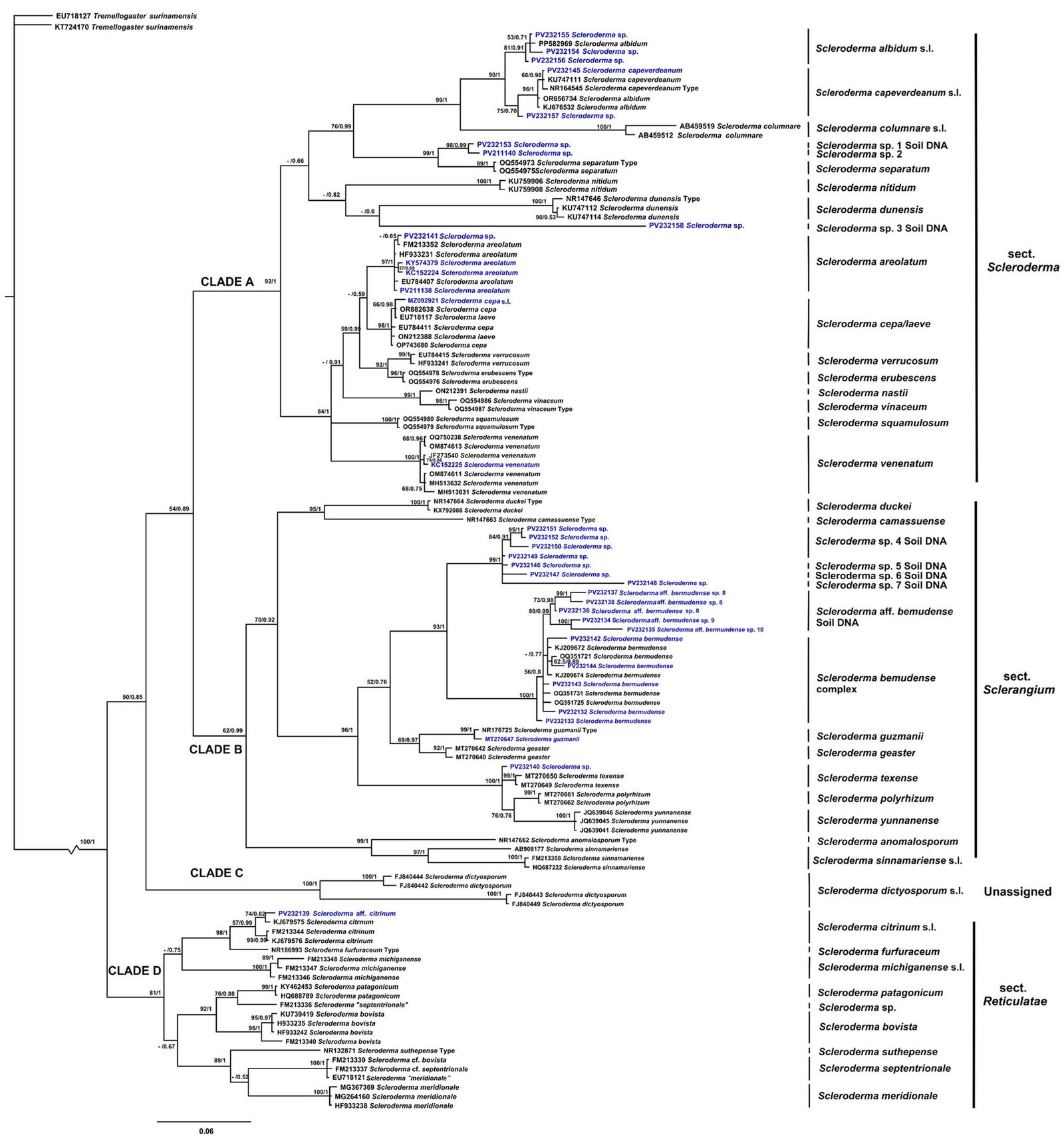
Table 2
Distribution and abundance of Scleroderma species obtained from soil samples.
| Species | Distribution | Abundance (Number of sequences) | Number of sites in Mexico |
| Scleroderma albidum s.l. | Estado de México | 5 | 1 |
| Scleroderma areolatum | Michoacán | 5 | 1 |
| Scleroderma bermudense | Quintana Roo and Yucatán | 164 | 2 |
| Scleroderma aff. bermudense sp. 8 | Morelos, Estado de México, Quintana Roo, and Yucatán | 3,877 | 5 |
| Scleroderma aff. bermudense sp. 9 | Yucatán | 1 | 1 |
| Scleroderma aff. bermudense sp. 10 | Yucatán | 10 | 1 |
| Scleroderma capeverdeanum s.l. | Hidalgo and Estado de México | 74 | 2 |
| Scleroderma aff. citrinum | Hidalgo | 1 | 1 |
| Scleroderma texense | Veracruz | 35 | 2 |
| Scleroderma sp. 1 | Veracruz | 3 | 1 |
| Scleroderma sp. 3 | Campeche and Quintana Roo | 3 | 2 |
| Scleroderma sp. 4 | Campeche, Michoacán and Yucatán | 33 | 8 |
| Scleroderma sp. 5 | Campeche and Yucatán | 33 | 5 |
| Scleroderma sp. 6 | Yucatán | 1 | 1 |
| Scleroderma sp. 7 | Campeche and Yucatán | 5 | 3 |
Table 3
Distribution of Scleroderma species in different types of vegetation.
| Species | Type of vegetation |
| Scleroderma albidum s.l. | Tropical coniferous forest |
| Scleroderma areolatum | Tropical broadleaf forest |
| Scleroderma bermudense | Subtropical broadleaf forest |
| Scleroderma aff. bermudense sp. 8 | Tropical broadleaf forest, subtropical broadleaf forest and tropical coniferous forest |
| Scleroderma aff. bermudense sp. 9 | Subtropical broadleaf forest |
| Scleroderma aff. bermudense sp. 10 | Subtropical broadleaf forest |
| Scleroderma capeverdeanum s.l. | Tropical coniferous forest and subtropical coniferous forest |
| Scleroderma aff. citrinum | Subtropical broadleaf forest |
| Scleroderma texense | Tropical coniferous forest |
| Scleroderma sp. 1 | Tropical coniferous forest |
| Scleroderma sp. 3 | Tropical broadleaf forest and subtropical broadleaf forest |
| Scleroderma sp. 4 | Tropical broadleaf forest, subtropical broadleaf forest, and tropical coniferous forest |
| Scleroderma sp. 5 | Tropical broadleaf forest and subtropical broadleaf forest |
| Scleroderma sp. 6 | Subtropical broadleaf forest |
| Scleroderma sp. 7 | Tropical broadleaf forest and subtropical broadleaf forest |
In the case of some OTUs of the S. bermudense complex, they could be considered endemic to Mexico, as they were only recorded at 1 sampling site. Other studies have reported that S. bermudense represents one of the most abundant endemic taxa in the Caribbean, mainly associated with Coccoloba uvifera (Bâ et al., 2024; Põlme et al., 2017). This association is mediated by the environmental stress of the coastal dunes where they develop, which causes a high specificity of the symbiosis (Bâ et al., 2024; Põlme et al., 2017). We found several clades of S. bermudense s.l.with high genetic differentiation not associated with Coccoloba species. Thus, there is a species complex associated with S. bermudense with an unsolved taxonomy and ecology in the Yucatán Peninsula.
Species such as S. areolatum and S. cepa have been recorded throughout the country through their basidiomes (Guzmán & Herrera, 1973; Guzmán et al., 2013). Scleroderma areolatum was reported from Durango, Guerrero, Hidalgo, Jalisco, México City, Michoacán, Nuevo León, Oaxaca, Puebla, and Veracruz (Guzmán & Herrera, 1973). Through ITS analysis it has been confirmed that S. cepa s.l. is an ectomycorrhizal symbiont of pecan trees in Chihuahua and Coahuila and that it is possibly a species complex (Sánchez-Ledesma et al., 2023). However, the type specimens of both species have not been sequenced, so it is important to carry out their type studies given the importance they can have in agroecosystems. In fact, species complexes indicating cryptic lineages in fungi are common (Sánchez-Ramírez, 2015) and may include taxa that can be morphologically distinguished, as well as cryptic species that are only discernible through molecular data, as this study found for the S. albidum, S. bermudense, and S. cepa complexes.
We recorded for the first time S. venenatum in Mexico, a species considered toxic in China (Zhang et al., 2020). The presence of this species in the country is particularly relevant given that some Scleroderma species are traditionally consumed in Mexico. For example, the consumption of S. laeve has been reported in Morelos and S. texense in Oaxaca (Cortés-Pérez et al., 2021; De Ávila et al., 1980). In contrast, S. venenatum was recorded in Querétaro and can be distinguished from edible species by its sessile, brown to grayish brown basidiomes and well-developed rhizomorphs (Zhang et al., 2020). Regarding the identity of the species that have been reported as edible in Mexico, their identification was only carried out with morphology and given their importance in cultural contexts, it would be advisable to obtain molecular data from the basidiomes to corroborate their identity.
A higher diversity of Scleroderma in the Transmexican Volcanic Belt shows that, while for other organisms the system represents a barrier or a filter, fungi use it as a corridor (Gómez-Reyes et al., 2018). In this region, the complex topography, habitat variability, and the convergence between Nearctic and Neotropical biota contribute to a higher diversity of fungal species in general (Cifuentes-Blanco et al., 1997) and in particular for Scleroderma.
Acknowledgements
The first author thanks the Secretaría de Ciencia, Humanidades, Tecnología e Innovación (Secihti) for the scholarship granted (CVU 415474) and the Instituto de Ciencias Biológicas, Universidad Autónoma de Ciencias y Artes de Chiapas (UNICACH) for all the facilities provided. This article contains part of the results of the PhD thesis project for the Doctorado en Ciencias en Biodiversidad y Conservación de Ecosistemas Tropicales (UNICACH). This research was funded by UNAM-PAPIIT IV200223 grant awarded to RGO.
References
Bâ, A. M., Séne, S., Manokari, M., Galardis, M. B., Sylla, S. N., Selosse, M. A. et al. (2024). Coccoloba uvifera L. associated with Scleroderma bermudense Coker: a pantropical ectomycorrhizal symbiosis used in restoring of degraded coastal sand dunes. Mycorrhiza, 34, 375–389. https://doi.org/10.1007/s00572-024-01170-8
Bandou, E., Lebailly, F., Muller, F., Dulormne, M., Toribio, A., Chabrol, J. et al. (2006). The ectomycorrhizal fungus Scleroderma bermudense alleviates salt stress in seagrape (Coccoloba uvifera L.) seedlings. Mycorrhiza, 16, 559–565. https://doi.org/10.1007/s00572-006-0073-6
Baseia, I. G., Silva, B. D. B., Ishikawa, N. K., Soares, J. V. C., Franca, I. F., Ushijima, S. et al. (2016). Discovery or extinction of new Scleroderma species in Amazonia? Plos One, 11, 1–19. https://doi:10.1371/journal.pone.0167879
Binder, M., & Bresinsky, A. (2002). Derivation of a polymorphic lineage of Gasteromycetes from boletoid ancestors. Mycologia, 94, 85–98. https://doi.org/10.1080/15572536.2003.11833251
Bonito, G. M., Gryganskyi, A. P., Trappe, J. M., & Vilgalys, R. (2010). A global meta-analysis of Tuber ITS rDNA sequences: species diversity, host associations and long-distance dispersal. Molecular Ecology, 19, 4994–5008. https://doi.org/10.1111/j.1365294X.2010.04855.x
Brock, P. M., Doring, H., & Bidartondo, M. I. (2009). How to know unknown fungi: the role of a herbarium. New Phytologist, 181, 719–724. https://doi.org/10.1111/j.1469-8137.2008.02703.x
Bullaín-Galardis, M. M., López-Sánchez, R. C., Pruneau, L., Eichler-Lobermann, B., Fall, F., & Bâ, A. M. (2024). Using the ectomycorrhizal symbiosis between Coccoloba uvifera L. and Scleroderma bermudense Coker to restore a degraded coastal sand dune in Cuba. Trees, 38, 127–138. https://doi.org/10.1007/s00468-023-02470-w
Burnham, K., & Anderson, D. (2002). Model selection and multimodel inference: a practical information-theoretic approach. New York: Springer.
Cho, S., Kwag, Y., Han, S., Lee, D., & Kim, C. (2022). Two new records of Scleroderma species (Sclerodermataceae, Boletales) in South Korea. The Korean Journal of Mycology, 50, 115–123. https://doi.org/10.4489/KJM.20220011
Cifuentes-Blanco, J., Villegas-Ríos, M., Villarreal-Ordaz, J. L., & Sierra Galván, S. (1997). Diversity of macromycetes in pine-oak forests in the Neovolcanic Axis, Mexico. In M. E. Palm, & I. H. Chapela (Eds.), Mycology in sustainable development: expanding concepts, vanishing borders (pp. 111–121). Boone, North Carolina: Parkway Publishers, Inc.
Conabio (Comisión Nacional para el Conocimiento y Uso de la Biodiversidad). (2008). Ecorregiones terrestres de México. Escala 1:1000000. México. Digital cartographic dataset. Mexico. https://www.conabio.gob.mx/informacion/gis/
Cortés-Pérez, A., Pérez-Pacheco, C. K., Yescas-Arreola, E., & Ramírez-Cruz, V. (2021). Primer registro de Scleroderma texense (Boletales, Sclerodermatinae) como una especie comestible en la Sierra Sur de Oaxaca, México. Scientia Fungorum, 52, 1–8. https://doi.org/10.33885/sf.2021.52.1386
Crous, P. W., Wingfield, M. J., Richardson, D. M., Le Roux, J. J., Strasberg, D., Edwards, J. et al. (2016). Fungal planet description sheets. Persoonia, 36, 316–458. https://doi:10.3767/003158516X692185.
Dai, Y. C., & Yang, Z. L. (2008). A revised checklist of medicinal fungi in China. Mycosystema, 27, 801–824.
Darriba, D., Taboada, G. L., Doallo, R., & Posada, D. (2012). jModelTest 2: more models, new heuristics and parallel computing. Nature Methods, 9, 772. http://doi:0.1038/nmeth.2109
De Ávila, A. B., Welden, A. L., & Guzmán, G. (1980). Notes on the ethnomycology of Hueyapan, Morelos, México. Journal of Ethnopharmacology, 2, 311–321. https://doi.org/10.1016/S0378-8741(80)81013-0
Felsenstein, J. (1985). Confidence limits on phylogenies: an approach using the bootstrap. Evolution, 39, 783–791. http//doi:10.1111/j.1558-5646.1985.tb00420.x
Fernández-Miranda, C. E. (2014). Hongos ectomicorrícicos de plantas leñosas en terrenos degradados de Asturias por actividad minera e industrial (Ph.D. Thesis). Universidad de Oviedo. Oviedo, España.
GBIF.org (2024). 27 August 2024 GBIF Occurrence Download https://doi.org/10.15468/dl.bbmwbt
Gómez-Reyes, V. M., Vázquez-Marrufo, G., Ortega-Gómez, A. M., & Guevara-Guerrero, G. (2018). Ascomicetos hipogeos de la región occidental del Sistema Volcánico Transversal, México. Acta Botanica Mexicana, 125, 37–48. https://doi.org/10.21829/abm125.2018.1327
Guzmán, G. (1967). Taxonomía del género Scleroderma Pers. emend. Fr. Ciencia, 2, 195–208.
Guzmán, G. (1970). Monografía del género Scleroderma Pers. emend. Fr. (Fungi-Basidiomycetes). Darwiniana, 16, 233–407.
Guzmán, G., & Herrera, T. (1973). Especies de macromicetos citadas de México IV. Gasteromicetos. Boletín de la Sociedad Mexicana de Micología, 2, 105–119.
Guzmán, G., Cortés-Pérez, A., Guzmán-Dávalos, L., Ramírez-Guillén, F., & Sánchez-Jácome, M. R. (2013). An emendation of Scleroderma, new records, and review of the known species in Mexico. Revista Mexicana de Biodiversidad, 84, 173–191. https://doi.org/10.7550/rmb.31979
Guzmán-Dávalos, L., & Guzmán, G. (1985). Hongos del estado de Jalisco, V. El género Scleroderma. Revista Mexicana de Micología, 1, 109–128.
Hawksworth, D. L. (1991). The fungal dimension of biodiversity: magnitude, significance and conservation, Mycological Research, 95, 641–655
Hawksworth, D. L., & Lücking, R. (2017). Fungal diversity revisited: 2.2 to 3.8 million species. Microbiology Spectrum, 5, 10–1128. https://doi.org/10.1128/microbiolspec.funk-0052-20
Heeger, F., Bourne, E. C., Baschien, C., Yurkov, A., Bunk, B., Spröer, C. et al. (2018). Long-read DNA metabarcoding of ribosomal RNA in the analysis of fungi from aquatic environments. Molecular Ecology Resources, 18, 1500–1514. http://doi.org/10.1111/1755-0998.12937
Karun, N. C., Mahadevakumar, S., & Sridhar, K. R. (2022). On the Scleroderma in southwest India. Species, 23, 297–312.
Kirk, P. M., Cannon, P. F., Minter, D. W., & Stalpers, J. A. (2008). Ainsworth & Bisby’s Dictionary of the Fungi (10ª Ed.). Wallingford, UK: CAB International.
Korpelainen, H., & Pietiläinen, M. (2017). Diversity of indoor fungi as revealed by DNA metabarcoding. Genome, 60, 55–64. http//doi.org/10.1139/gen-2015-0191
Kumla, J., Suwannarach, N., Bussaban, B. & Lumyong, S. (2013). Scleroderma suthepense, a new ectomycorrhizal fungus from Thailand. Mycotaxon, 123, 1–7. http//doi.org/10.5248/123.1
Lu, X., Malajczuk, N., & Dell, B. (1998). Mycorrhiza formation and growth of Eucalyptus globulus seedlings inoculated with spores of various ectomycorrhizal fungi. Mycorrhiza, 8, 81–86. https://doi.org/10.1007/s005720050216
Montagner, D. F., Coelho, G., Silveira, A. O., Baldoni, D. B., & Antoniolli, Z. (2015). Morphological and molecular analyses in Scleroderma (Basidiomycota) associated with exotic forests in Pampa biome, southern Brazil. Mycosphere, 6, 337–344. https://doi.org/10.5943/mycosphere/6/3/9
Nouhra, E. R., Hernández, C. M. L., Pastor, N., & Crespo, E. M. (2012). The species of Scleroderma from Argentina, including a new species from the Nothofagus forest. Mycologia, 104, 488–495. https://doi.org/1 0.3852/11-082
Ortiz-Rivero, J., Watling, R., Guzmán-Dávalos, L., & Martín, M. P. (2021). The many-rooted earthball-Scleroderma geaster and S. polyrhizum revisited, with the description of a new species. Phytotaxa, 510, 1–17. https://doi.org/10.11646/phytotaxa.510.1.1
Pera, J., & Parladé, J. (2005). Inoculación controlada con hongos ectomicorrícicos en la producción de planta destinada a repoblaciones forestales: estado actual en España. Sistemas y Recursos Forestales, 14, 419–433.
Persoon, C. H. (1801). Synopsis methodica Fungorum. Göttingen: Henricus Dieterich.
Phosri, C., Martín, M. P., Watling, R., Jeppson, M., & Sihanonth, P. (2009). Molecular phylogeny and re-assessment of some Scleroderma spp. (Gasteromycetes). Anales del Jardín Botánico de Madrid, 66, 83–91.
Põlme, S., Bahram, M., Kõljalg, U., & Tedersoo, L. (2017). Biogeography and specificity of ectomycorrhizal Fungi of Coccoloba uvifera. In L. Tedersoo (Ed.), Biogeography of mycorrhizal symbiosis. Ecological studies (pp 345–360). Cham, Switzerland: Springer.345https://doi.org/10.1007/978-3-319-56363-3_16
Rambaut, A. (2018). FigTree v1.4.4. Institute of Evolutionary Biology, University of Edinburgh. http://tree.bio.ed.ac.uk/software/figtree/
Rambaut, A., Drummond, A. J., Xie, D., Baele, G., & Suchard, M. A. (2018). Posterior summarization in Bayesian phylogenetics using tracer 1.7. Systematic Biology, 67, 901–904. https://doi.org/10.1093/sysbio/syy032
Rebriev, Y. A., & Zvyagina, E. A. (2022). Scleroderma furfuraceum (Boletales, Agaricomycetes) a new species from the Russian Far East. Phytotaxa, 555, 169–177. https://doi.org/10.11646/phytotaxa.555.2.5
Rincón, A., Álvarez, I. F., & Pera, J. (2001). Inoculation of containerized Pinus pinea L. seedlings with seven ectomycorrhizal fungi. Mycorrhiza, 11, 265–271.
Ruankaew-Disyatat, N., Yomyart, S., Sihanonth, P., & Piapukiew, J. (2016). Community structure and dynamics of ectomycorrhizal fungi in a dipterocarp forest fragment and plantation in Thailand. Plant Ecology & Diversity, 9, 577–588. https://doi.org/10.1080/17550874.2016.1264018
Ruiz-González, L. E., Vázquez-Zea, J. A., Vega-Villasante, F., Guzmán-Davalos, L., & Guerrero-Galván, S. R. (2017). Evaluation of the toxicity of Basidiomycota fungi on the hatching of Artemia franciscana cysts. Revista Iberoamericana de Micologia, 34, 220–224. https://doi.org/10.1016/j.riam.2017.03.007
Rusevska, K., Karadelev, M., Phosri, C., Dueñas, M., Watling, R., & Martín, M. P. (2014). Rechecking of the genus Scleroderma (Gasteromycetes) from Macedonia using barcoding approach. Turkia Journal of Botany, 38, 375–385. http//doi.org/10.3906/bot-1301-36
Sánchez-Ledesma, J. A., Garibay-Orijel, R., Guevara-Guerrero, G., Ávila-Rodríguez, V., & Arreola-Ávila, J. G. (2023). Macromicetos asociados con Carya illinoinensis en la Comarca Lagunera, México. Revista Mexicana de Biodiversidad, 94, e944074. https://doi.org/10.22201/ib.20078706e.2023.94.4074
Sánchez-Ramírez, S. (2015). Scaling macro and micro evolutionary dynamics in the Caesar’s mushrooms (Amanitasect. Caesareae) (Ph.D. Thesis). University of Toronto, Canada.
Sanon, K. B., Bâ, A. M., Delaruelle, C., Duponnois, R., & Martin, F. (2009). Morphological and molecular analyses in Scleroderma species associated with some Caesalpinioid legumes, Dipterocarpaceae and Phyllanthaceae trees in southern Burkina Faso. Mycorrhiza, 19, 571–584. https://doi.org/10.1007/s00572-009-0272-z
Santolamazza-Carbone, S., Iglesias-Bernabé, L., Sinde-Stompel, E., & Gallego, P. P. (2023). Soil microbiota impact on Boletus edulis mycelium in chestnut orchards of different ages. Applied Soil Ecology, 185, 104790. https://doi.org/10.1016/j.apsoil.2022.104790
Sato, Y., Tomonari, H., Kaneko, Y., & Yo, K. (2020). Mushroom poisoning with Scleroderma albidum: a case report with review of the literature. Acute Medicine & Surgery, 7, e460. https://doi:10.1002/ams2.460
Sayers, E. W., Cavanaugh, M., Clark, K., Pruitt, K. D., Sherry, S. T., Yankie, L., & Karsch-Mizrachi, I. (2024). GenBank 2024 update. Nucleic Acids Research, 52, D134–D137. https://doi.org/10.1093/nar/gkad903
Sims, K. P., Watling, R., & Jeffries, P. (1995). A revised key to the genus Scleroderma. Mycotaxon, 56, 403–420. https://doi.org/10.5962/p.415939
Tao, J., Wang, X., Long, Y., Gao, Z., Zhang, G., Guo, Z. et al. (2024). Determining gene order patterns in the Suillus and Boletales through comparative analysis of their mitogenomes. International Journal of Molecular Sciences, 25, 9597. https://doi.org/10.3390/ijms25179597
Tedersoo, L., & Anslan, S. (2019). Towards PacBio-based pan-eukaryote metabarcoding using full-length ITS sequences. Environmental Microbiology Reports, 11, 659–668. https://doi.org/10.1111/1758-2229.12776
Tedersoo, L., Bahram, M., Põlme, S., Kõljalg, U., Yorou, N. S., Wijesundera, R. et al. (2014). Global diversity and geography of soil fungi. Science, 346, 1078–1089. https://doi.org/10.1126/science.1256688
Tedersoo, L., Bahram, M., Zinger, L., Nilsson, R. H., Kennedy, P. G., Yang, T. et al. (2022). Best practices in metabarcoding of fungi: from experimental design to results. Molecular Ecology, 31, 2769–2795. https://doi.org/10.1111/mec.16460
Tedersoo, L., Mikryukov, V., Anslan, S., Bahram, M., Khalid A. N., Corrales, A. et al. (2021). The Global Soil Mycobiome consortium dataset for boosting fungal diversity research. Fungal Diversity, 111, 573–588. https://doi.org/10.1007/s13225-021-00493-7
Truong, C., Mujic, A. B., Healy, R., Kuhar, F., Furci, G., Torres, D.et al.(2017). How to know the fungi: combining field inventories and DNA-barcoding to document fungal diversity. New Phytologist, 214, 913–919. https://doi.org/10.1111/nph.14509
Valdés-Ramírez, M., Ambriz-Parra, E., Camacho-Vera, A., & Fierros-González, A. M. (2010). Inoculación de plántulas de pinos con diferentes hongos e identificación visual de la ectomicorriza. Revista Mexicana de Ciencias Forestales, 1, 53–63.
Wang, X., Liu, P., & Yu, F. (2004). Color atlas of wild commercial mushrooms in Yunnan. Kunming: Yunnan Science and Technology Press.
Wilson, A. W., Binder, M., & Hibbett, D. S. (2012). Diversity and evolution of ectomycorrhizal host associations in the Sclerodermatineae (Boletales, Basidiomycota). New Phytologist, 194, 1079–1095. https://doi:10.1111/j.1469-8137.2012.04109.x
Wilson, A.W., Binder, M., & Hibbett, D. S. (2011). Effects of gasteroid fruiting body morphology on diversification rates in three independent clades of fungi estimated using binary state speciation and extinction analysis.
Evolution, 65, 1305–322. https://doi.org/10.1111/j.1558-5646.2010.01214.x.
Wu, R., Zhou, L., Qu, H., & Ge, Z. W. (2023). Updates on Scleroderma: four new species of section Scleroderma from Southwestern China. Diversity, 15, 775. https://doi.org/10.3390/d15060775
Yang, K. L., Lin, J. Y., Li, G. M., & Yang, Z. L. (2025). Updates of Scleroderma (Basidiomycota, Boletales): new data from 18 selected species in China. Phytotaxa, 706, 209–254. https://doi.org/10.11646/phytotaxa.706.3.3
Yao, Q., Wu, Z., Zhong, J., Yu, C., Li, H., Hu, Q. et al. (2023). A network system for the prevention and treatment of mushroom poisoning in Chuxiong Autonomous Prefecture, Yunnan Province, China: implementation and assessment. BMC Public Health, 23, 1979. https://doi.org/10.1186/s12889-023-16042-7
Zhang, C., Xu, X., & Liu, J. (2013). Scleroderma yunnanense, a new species from South China, in Mycotaxon, 125, 193–200. https://doi.10.5248/125.193
Zhang, Y. Z., Sun, C.Y., Sun, J., Zhang, K. P., Zhang, H. S., Guo, X. et al. (2020). Scleroderma venenatum sp. nov., S. venenatum var. macrosporum var. nov. and S. suthepense new to China. Phytotaxa, 438, 107–118. https://doi.org/10.11646/phytotaxa.438.2.4
Zhong, J., Li H., Zhang, Y., Yu C., Pu, Y., Peng, J. et al. (2021). An investigation of food poisoning by mistaken eating of Scleroderma cepa. Chinese Journal of Food Hygiene, 33, 616–619.

Caracterización y ordenación del matorral de Juniperus angosturana del Valle del Mezquital, Hidalgo
Characterization and ordination of the Juniperus angosturana scrub in the Mezquital Valley, Hidalgo
Sarahí Flores-Martínez a, Ro Linx Granados-Victorino b, Diódoro Granados-Sánchez a, *, Enrique Guízar-Nolazco a, Alejandro Corona-Ambriz a, Saúl Castañeda-Díaz b y Joaquín Parra-Álvarez c
a Universidad Autónoma Chapingo, División de Ciencias Forestales, Carretera México-Texcoco, Km 38.5, 56230 Chapingo, Texcoco, Estado de México, México
b Universidad Autónoma Chapingo, Área de Biología, Departamento de Preparatoria Agrícola, Carretera México-Texcoco Km 38.5, 56230 Chapingo, Texcoco, Estado de México, México
c Universidad Autónoma Chapingo, Área de Agronomía, Departamento de Preparatoria Agrícola, Carretera México-Texcoco, Km 38.5, 56230 Chapingo, Texcoco, Estado de México, México
*Autor para correspondencia: dgranadoss@chapingo.mx (D. Granados-Sánchez)
Recibido: 13 julio 2025; aceptado: 22 octubre 2025
Resumen
Juniperus angosturana R.P. Adams, es una especie endémica de México que ha sido escasamente estudiada desde una perspectiva ecológica. Su límite sur de distribución geográfica se ubica en el Valle del Mezquital, una región con fuerte presión antrópica. Bajo este contexto, en este estudio se analizó la composición y estructura de las comunidades dominadas por Juniperus angosturana, con el fin de comprender los factores ambientales que influyen en su fisonomía. Para describir la estructura de la vegetación de estas comunidades, se empleó el método de cuadrantes centrados en un punto, mediante el cual se calcularon los valores estructurales de especies arbustivas y arbóreas. La delimitación de asociaciones vegetales se realizó mediante un análisis de agrupamiento. Así mismo, se aplicó un análisis de correspondencias canónicas para evaluar la influencia de variables ambientales y edáficas en la estructura y la composición florística. Como resultados, se identificaron 4 asociaciones dominadas por Juniperus angosturana, cuya diferenciación estructural mostró una alta correlación con las características del suelo, en particular con la textura, concentraciones de calcio, potasio y fósforo, así como con el pH.
Palabras clave: Asociaciones vegetales; Zonas áridas; Sinecología; Enebro; Análisis estructural
Abstract
Juniperus angosturana R.P. Adams is a species endemic to Mexico that has been little studied from an ecological perspective. Its southern geographical distribution limit is located in the Mezquital Valley, a region subject to strong anthropogenic pressure. In this context, this study analyzed the composition and structure of communities dominated by J. angosturana in order to understand the environmental factors that influence their appearance. To describe the vegetation structure of these communities, the point-centered quadrant method was used to calculate the structural values of shrub and tree species. Plant associations were delimited using cluster analysis. Likewise, a Canonical Correspondence Analysis was applied to evaluate the influence of environmental and edaphic variables on the structure and floristic composition. As a result, 4 associations dominated by Juniperus angosturana were identified, whose structural differentiation showed a strong correlation with soil characteristics, particularly texture, calcium, potassium, and phosphorus concentrations, as well as pH.
Keywords: Plant associations; Arid zones; Synecology; Juniper; Structural analysis
Introducción
La vegetación asociada a climas áridos y semiáridos se distribuye en varias regiones que abarcan más de la mitad del territorio mexicano (Pérez-Aguilar et al., 2021). Estas regiones presentan una gran diversidad de matorrales cuya composición y estructura varían de una zona a otra, y son ecosistemas clave para la conservación de la biodiversidad. En todos los tipos de matorrales destacan las formas de vida arbustivas por su dominancia, biomasa y su efecto en el ambiente y otras especies (González-Medrano, 2012; Rzedowski, 2006).
En términos ecológicos las especies de Juniperus L. desempeñan un papel fundamental en las zonas áridas, ya que contribuyen a la formación, protección y retención del suelo (Allegrezza et al., 2016; Romo et al., 2012), así como a la conservación de la biodiversidad al funcionar como refugio o como alimento para la fauna silvestre (Fonseca, 2006). Además, dichas especies facilitan la germinación de semillas de otras plantas al formar sitios seguros de germinación o “islas de recursos” (Miwa y Reuter, 2010; Villanueva-Díaz et al., 2016). Su alta adaptabilidad a condiciones ambientales adversas —como la tolerancia a las sequías, al fuego, a temperaturas extremas o la capacidad de crecer en suelos pobres— las convierte en especies clave para la restauración ecológica (Herrerías y Nieto, 2020).
Juniperus angosturana R.P. Adams (sinónimo: Juniperus monosperma var. gracilis Mart) es una especie arbustiva endémica de México con copas irregulares o redondeadas, que puede alcanzar hasta 2 m de altura y en condiciones idóneas específicas, hasta 7 m. Se desarrolla en regiones de clima templado semiseco, donde forma parte de pastizales, matorrales y bosques bajos escuamifolios (Rzedowski, 2006). Su distribución altitudinal varía entre 1,300 y 2,000 m snm y abarca la fachada occidental de la sierra Madre Oriental desde Coahuila y Nuevo León y el altiplano mexicano en San Luis Potosí y Guanajuato —donde establece asociaciones vegetales con Pinus cembroides Zucc. subsp. cembroides Zucc., particularmente en zonas afectadas por disturbios ecológicos (Estrada-Castillón et al., 2014)— hasta Hidalgo, en el Valle del Mezquital, límite sur de su distribución.
El Valle del Mezquital se ha caracterizado por una intensa actividad humana y cambios en el uso de suelo, lo cual ha provocado una disminución significativa de la cobertura forestal. Entre las causas principales se encuentran el sobrepastoreo, la labranza postcosecha y el manejo inadecuado del suelo agrícola (Hernández-González et al., 2018). Dado que las zonas áridas y semiáridas son especialmente sensibles al disturbio antropogénico (González-Medrano, 2012), es importante conocer la dinámica ecológica de estos matorrales con la finalidad de evitar su degradación progresiva. La caracterización y ordenación de los matorrales dominados por J. angosturana constituye una necesidad para analizar los factores que determinan su estructura y composición florística, a su vez, desarrollar estrategias pertinentes de manejo, conservación y aprovechamiento racional de la especie y de los ecosistemas en los que se encuentra.
El objetivo del presente trabajo fue caracterizar las asociaciones vegetales dominadas por J. angosturana en el Valle del Mezquital, Hidalgo, y por medio de la técnica de ordenación, definir la relación entre la estructura y los factores ambientales y edáficos. El estudio también proporciona bases técnicas y ecológicas para orientar las acciones concretas de conservación y manejo sustentable de los matorrales donde esta especie actúa como elemento estructural dominante.
Materiales y métodos
La presente investigación se realizó en el límite sur de la distribución geográfica de J. angosturana (GBIF, 2023; Natusfera, s.f.; EncicloVida, s.f.). Las localidades de colecta fueron La Florida y San Cristóbal, pertenecientes al municipio Cardonal, ubicado en el Valle del Mezquital, al noreste de Hidalgo (fig. 1), dentro del altiplano central mexicano y de la provincia fisiográfica de la Meseta Neovolcánica, ahora Faja Volcánica Transmexicana (Hernández-Armas, 2016). La zona de estudio se localiza a una altitud promedio de 2,040 m snm, los climas presentes son el templado subhúmedo con lluvias en verano (Cw1), el semiseco templado (BS1kw), semiseco semicálido (BS0hw) y seco semicálido (BS0h). La vegetación de la zona se compone de bosques de pino y encino, matorral xerófilo, pastizales y áreas destinadas a la agricultura (INEGI, 2009, en Guzmán-Cornejo et al., 2015). La precipitación anual promedio es de 409 mm y la temperatura promedio es de 18 °C (Hernández-Armas, 2016).
Se realizaron recolectas botánicas generales estacionales durante los meses de octubre de 2023 y abril, junio, agosto y noviembre de 2024, con la finalidad de obtener muestras de especies perennes y anuales. Los ejemplares recolectados fueron herborizados para su determinación taxonómica mediante el uso de claves especializadas y consultas con expertos, para finalmente ser integrados a colecciones de herbario. En total se revisaron 143 ejemplares recolectados por Enrique Guízar Nolazco (núms. 7981-8123, excepto 7997 y 8022) y Rubén Herrera Flores, depositados en CHAP herbario de la Universidad Autónoma Chapingo, con duplicados de 7981, 7982, 7986, 7992, 7994, 7995, 8015, 8023, 8025, 8027, 8030, 8031, 8039, 8040, 8042, 8045, 8069, 8072, 8076, 8080, 8082, 8083, 8111, 8113, 8114, 8115a y 8119 en UAMIZ herbario de la Universidad Autónoma Metropolitana Unidad Iztapalapa. La nomenclatura de los nombres científicos se basó en la propuesta del International Plant Name Index (IPNI, 2025).
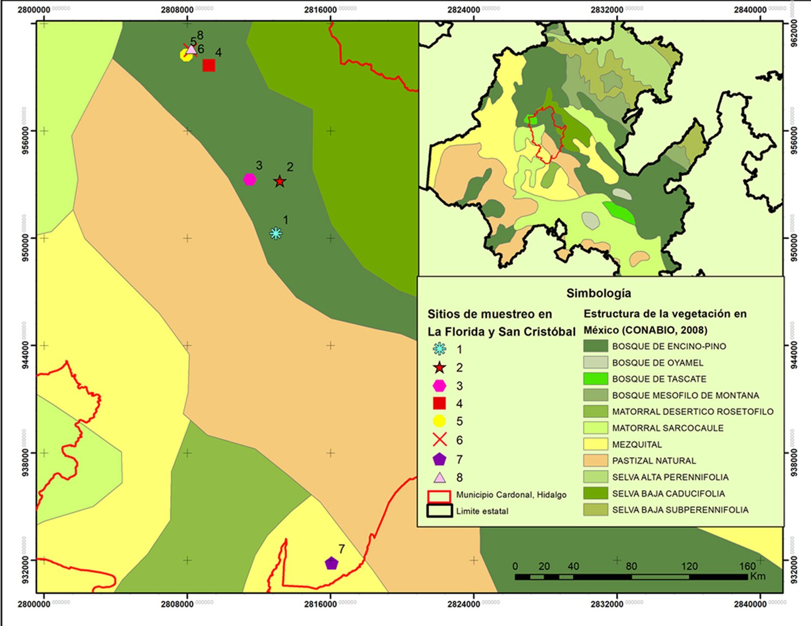
En total se tomaron muestras de 8 sitios, 4 en cada localidad. Para cada sitio se registraron las siguientes variables ambientales: exposición —determinada con una brújula —, pendiente del terreno —medida con un clinómetro Suunto— y altitud —registrada mediante una antena GPS Garmin eTrex 20x. Para determinar las condiciones edáficas, en cada sitio se recolectó una muestra de ~1 kg de suelo, previa remoción de la hojarasca superficial. Posteriormente, se realizaron las siguientes determinaciones: pH, materia orgánica (MO), nitrógeno inorgánico (N inorg.), fósforo asimilable (P), potasio (K), calcio (Ca), hierro (Fe), así como los porcentajes de limo, arena y arcilla, con los que se determinó la textura del suelo (TEX).
Para describir la estructura de la vegetación se utilizó el método de cuadrantes centrados en un punto utilizado por Granados-Victorino et al. (2015), método que no depende de un área delimitada y se basa en las distancias entre puntos fijos y los individuos más cercanos en cada cuadrante. En cada sitio se establecieron 10 puntos de muestreo, con una distancia de 20 m entre sí. En cada punto de muestreo se trazaron, de manera teórica, 4 cuadrantes a partir de ejes perpendiculares (en forma de plano cartesiano). En cada cuadrante se registró la distancia del punto central hasta el árbol o arbusto más cercano con una altura igual o mayor a un metro.
Los individuos registrados fueron identificados taxonómicamente, se midió su altura, con un flexómetro para aquellos individuos menores a 1.50 m y con un clinómetro para especies de porte mayor. Se estimó la cobertura de copa promediando 2 medidas de diámetro de la copa, tomadas en dirección norte-sur y este-oeste. Con los datos obtenidos y siguiendo la metodología propuesta por Cottam y Curtis (1956), modificada por Alanís-Rodríguez et al. (2020), se calcularon los valores relativos de abundancia, dominancia y frecuencia de las especies registradas. A partir de estos parámetros, se estimó el índice de valor de importancia relativa (VIR), el cual permite determinar la relevancia estructural de cada especie en la comunidad.
Con base en el VIR de cada especie, se realizó un análisis de agrupamiento utilizando el índice de disimilitud de Bray-Curtis como medida de distancia y el algoritmo de unión por promedio entre grupos (UPGMA). El índice de disimilitud de Bray-Curtis se utiliza para comparar la composición entre sitios e ignora los casos en los que las especies están ausentes, utiliza los valores del VIR (Rocha-Ramírez et al., 2013). A partir de un nivel de corte de 55% de la información retenida en el dendrograma, se identificaron los sitios con mayor semejanza estructural y se definieron las asociaciones vegetales dominantes.
La nomenclatura de las asociaciones vegetales se definió con base en las especies con mayor VIR en los grupos formados a partir del análisis de agrupamiento, así como la fisionomía general de las especies dominantes, de acuerdo con lo sugerido en González-Medrano (2004). Para representar gráficamente la estructura vertical y horizontal de estas asociaciones, se elaboró un perfil semirrealista de la vegetación del transecto de estudio, tomando como base los valores estructurales obtenidos. El análisis de ordenación se realizó mediante un análisis de correspondencias canónicas (ACC), que consiste en una regresión múltiple donde se relacionó el VIR de las especies con las variables ambientales y edáficas registradas. Ambos análisis se llevaron a cabo con el software Past v.4.03 (Hammer et al., 2001).
Resultados
Se identificaron 89 especies en las comunidades vegetales con presencia de Juniperus angosturana en el Valle del Mezquital, que pertenecen a 73 géneros y 41 familias. Las familias más representativas fueron Asteraceae con 10 especies, seguida de Cactaceae y Fabaceae con 8 especies cada una y Asparagaceae con 7. La localidad con mayor riqueza especifica fue La Florida con 72 especies.
Juniperus angosturana se desarrolla principalmente en matorrales, aunque también puede figurar como un elemento importante en los bosques de coníferas de las zonas semiáridas, en especial en aquellos dominados por pinos piñoneros y enebros (Juniperus spp.) (Romme et al., 2009). En las localidades del Valle del Mezquital se reconocieron 4 tipos de vegetación (tabla 1) y 4 asociaciones vegetales con presencia de J. angosturana, las cuales presentan diferencias estructurales y florísticas (figs. 2, 3). A continuación, se describen las características de cada una de dichas asociaciones: a) asociación Juniperus angosturana – Juniperus flaccida Scltdl. Esta asociación vegetal se encuentra en la localidad de San Cristóbal, en específico en los sitios 4 y 5, en altitudes que oscilan entre 1,970 y 2,070 m, con pendiente de 10 a 20% y exposición noroeste. Los suelos son pedregosos, con textura franco-arcillosa, moderadamente alcalinos, con bajo contenido de MO y altas concentraciones de Ca. La comunidad vegetal es codominada por Juniperus angosturana y Juniperus flaccida Schltdl., con VIR de 44% y 31%, respectivamente. Se trata de un bosque con baja densidad arbórea, en el que predominan los individuos de porte bajo que no sobrepasan 4 metros de altura, en cuyos claros es común la presencia de arbustos. Otras especies que se pueden encontrar son Agave lechuguilla Torr., Agave salmiana Otto ex Salm-Dyck var. salmiana, Berberis pallida Benth., Calliandra eriophylla Benth., Cercocarpus fothergilloides Kunth, Chrysactinia mexicana A. Gray, Cylindropuntia imbricata (Haw.) F.M. Knuth, Dalea bicolor Humb. et Bonpl. ex Willd., Dalea greggii A. Gray, Echinocactus platyacanthus Link et Otto, Ferocactus latispinus (Haw.) Britton et Rose, Flourensia resinosa (T. S. Brand.) Blake, Malacomeles denticulata (Kunth) Decne., Mammillaria sp., Milla biflora Cav., Opuntia rastrera F. A. C. Weber, Opuntia robusta H.L. Wendl. ex Pfeiff., Opuntia tomentosa Salm-Dyck, Perymenium mendezii DC., Sanvitalia procumbens Lam., Senna guatemalensis var. hidalgensis H. S. Irwin et Barneby, Thymophylla setifolia Lag., así como algunos individuos de Pinus cembroides Zucc, en las zonas más elevadas (fig. 4A). b) Asociación Juniperus angosturana – Pinus cembroides, se registró en los sitios 6 y 8 de San Cristóbal, entre 1,985 y 2,080 m snm, en pendientes de 10 a 30% y exposición noreste. Juniperus angosturana presentó el VIR más alto con 29%. El estrato arbóreo está compuesto por P. cembroides (21%), J. flaccida (5%) y Pinus pinceana Gordon et Glend (4.6%), conforman un dosel cuya altura varía entre 2 y 6 m. Además de J. angosturana, el estrato arbustivo incluye Ephedra compacta Rose, Rhus schiedeana Schltdl. y Rhus standleyi F.A. Barkley. Asimismo, se registraron especies como Agave lechuguilla, Agave salmiana var. salmiana, Chrysactinia mexicana, Electranthera mutica (DC.) Mesfin, D.J. Crawford et Pruski, Cylindropuntia imbricata, Dalea greggii, Flourensia resinosa, Milla biflora, Opuntia rastrera, Opuntia tomentosa, Perymenium mendezii, Sanvitalia procumbens, y Zinnia peruviana (L.) L. Este matorral se desarrolla sobre suelos pedregosos, con pH alcalino, de textura franco-arcillo-arenosa y con una elevada concentración de Ca y Fe (fig. 4B). c) Juniperus angosturana – Nolina parviflora. En esta asociación vegetal J. angosturana es la especie estructuralmente dominante, con un VIR de 57%. Coexiste con P. cembroides, Nolina parviflora (Kunth) Hemsl, J. flaccida, Dasylirion longissimum Lem., Agave salmiana Otto ex Salm-Dyck var. salmiana, Echinocactus platyacanthus Link et Otto, Ephedra compacta y diversas especies del género Opuntia. El estrato arbustivo no supera los 2 m de altura y en el estrato arbóreo los individuos más grandes llegan a medir hasta 5 m. Esta asociación, se distribuye en La Florida, específicamente en los sitios 1, 2 y 7, en altitudes que van de 1,800 a 2,050 m, en laderas con exposición sureste y pendientes de 7 a 30%. Los suelos son poco desarrollados, cuentan con una delgada capa de hojarasca y fragmentos sueltos de roca; presentan bajo contenido de materia orgánica (8%) y un pH de entre 7 y 8, y son ricos en Ca y K. Otras especies registradas fueron: Agave lechuguilla, Chrysactinia mexicana, Electranthera mutica, Cylindropuntia imbricata, Dahlia coccinea Cav., Dalea bicolor, Flourensia resinosa, Gochnatia hypoleuca (DC.) A. Gray, Lysiloma sp., Mammillaria sp., Milla biflora, Opuntia rastrera, Opuntia tomentosa, Perymenium mendezii DC., Sanvitalia procumbens, Sclerocarpus uniserialis, Thymophylla setifolia y Zinnia peruviana (fig. 4C). d) Juniperus angosturana – Neltuma laevigata, se registró únicamente en un sitio de muestreo, en La Florida, a una altitud promedio de 2,000 m, con una pendiente de 25% y exposición sureste. El suelo presenta una textura fina franco-arcillosa, y una alcalinidad ligera. Según los VIR, Juniperus angosturana es la especie dominante en el estrato arbustivo, con valor de 36% y alturas inferiores de 3 m. En el estrato arbóreo, con un dosel de entre 2 y 6 m de altura, destacan las especies Senegalia berlandieri Benth. y Neltuma laevigata (Humb. y Bonpl. ex Willd.) Britton y Rose,con un VIR conjunto de 25%. Asimismo, se registraron otras especies como Cylindropuntia imbricata, Cylindropuntia leptocaulis (DC.) F.M. Knuth, Milla biflora, Opuntia tomentosa, Jatropha dioica Sessé ex Cerv., Sclerocarpus uniserialis (Hook.) Benth. et Hook. f. ex Hemsl., Senna holwayana (Rose) I. et Barneby, Uncaria tomentosa (Willd. ex Schult.) DC. y Yucca filifera Chabaud (fig. 4D).
Tabla 1. Clasificación de la vegetación en las localidades La Florida y San Cristóbal en Cardonal, Hidalgo, basado en lo propuesto por González-Medrano (2004) para la vegetación de México.
| Categoría | Denominación |
| Tipo de vegetación | Bosque bajo de escuamifolios |
| Asociación | Juniperus angosturana – Juniperus flaccida |
| Tipo de vegetación | Bosque bajo de aciculifolios |
| Asociación | Juniperus angosturana – Pinus cembroides |
| Tipo de vegetación | Matorral mediano rosetófilo |
| Asociación | Juniperus – Nolina parviflora |
| Tipo de vegetación | Bosque bajo espinoso |
| Asociación | Juniperus angosturana – Neltuma laevigata |
Con base en los resultados obtenidos, las especies de mayor importancia ecológica en las asociaciones, además de J. angosturana, son P. cembroides, J. flaccida, Senegalia berlandieri,Neltuma laevigata y Nolina parviflora,las cuales presentaron los valores de importancia relativa más altos en las localidades muestreadas. La dominancia de Juniperus angosturana se atribuye principalmente a su mayor diámetro de copa, más que a su altura, en comparación con las demás especies representativas. La asociación más observada fue la de Pinus cembroides-Juniperus angosturana, seguida de J. angosturana-J. flaccida. Ambas asociaciones vegetales presentan acompañamiento de especies típicas de matorral xerófilo.
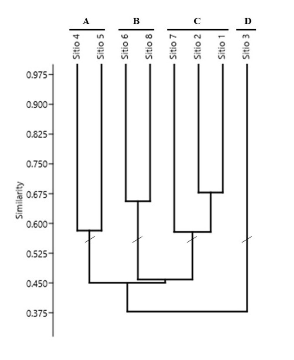
La diferenciación estructural de las asociaciones vegetales dominadas por Juniperus angosturana responde a un origen multifactorial y tiene una correlación, principalmente, con las variables edáficas (fig. 5). De acuerdo con el ACC, esta variación es explicada en 67.13% por los 3 primeros ejes (tablas 2, 3). Las variables edáficas más influyentes son la textura del suelo —en especial los porcentajes de arena y limo—, las concentraciones de Ca, K y P, así como el pH del suelo (tabla 2).
Discusión
Juniperus angosturana es una especie endémica de México, cuya distribución se extiende desde Coahuila hasta Hidalgo. A pesar de su relevancia estructural en las zonas áridas del país, ha sido escasamente estudiada desde una perspectiva ecológica. La mayoría de los trabajos publicados se han centrado en análisis filogenéticos (Adams, 1994; Adams y Schwarzbach, 2013; Uckele et al., 2021), en descripciones morfológicas y de distribución geográfica (Estrada-Castillón et al., 2014; Farjon, 2019; González-Elizondo et al., 2012), así como en modelos de distribución potencial o modelados de panbiología (Cartereau, et al., 2023; Morales-Garduño et al., 2021; Trájer, 2023).
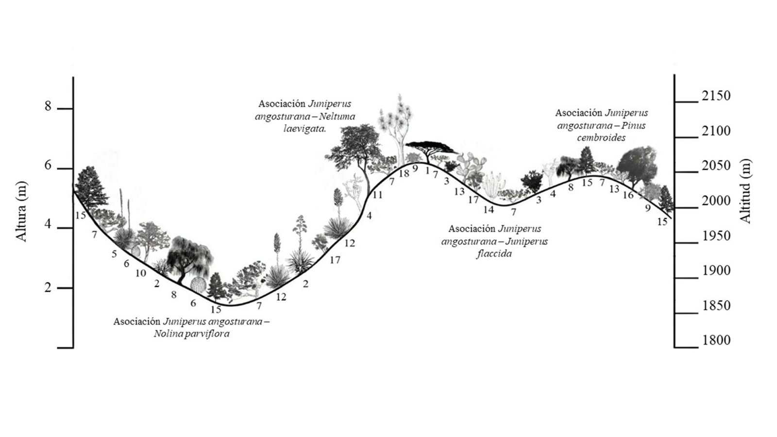
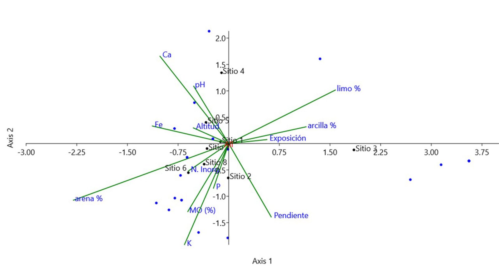
Tabla 2. Resultados de los primeros tres ejes de ordenación, de acuerdo con el análisis de correspondencias canónicas (ACC). Los valores en negritas señalan las variables con mayor peso en la definición de cada eje.
| Variable | Eje 1 | Eje 2 | Eje 3 |
| pH | -0.172893 | 0.36276 | 0.658303 |
| MO (%) | -0.202071 | -0.429806 | -0.215268 |
| N inorg. | -0.199503 | -0.173747 | 0.0472623 |
| P | -0.0753286 | -0.282118 | -0.700757 |
| K | -0.218424 | -0.638471 | -0.248518 |
| Ca | -0.339255 | 0.552029 | -0.00914643 |
| Fe | -0.377003 | 0.110919 | -0.443264 |
| arena (%) | -0.766368 | -0.357859 | 0.0899592 |
| limo (%) | 0.526614 | 0.338468 | 0.363971 |
| arcilla (%) | 0.381808 | 0.105922 | -0.377697 |
| Pendiente | 0.20969 | -0.463599 | 0.177899 |
| Exposición | 0.18856 | 0.0252954 | -0.295587 |
| Altitud | -0.174418 | 0.0991923 | -0.140028 |
| Distribución de la varianza | |||
| Valor propio | 0.521 | 0.364 | 0.318 |
| Varianza (%) | 29.07 | 20.3 | 17.76 |
| Varianza acumulada (%) | 29.07 | 49.37 | 67.13 |
Tabla 3. Matriz de correlación entre las variables ambientales y edáficas de los sitios de muestreo en Cardonal, Hidalgo. La parte superior derecha muestra los valores del coeficiente de correlación (r) y la diagonal inferior izquierda los valores de p (< 0.05)
| pH | MO (%) | N (inorgánico) | P | K | Ca | Fe | arena % | limo % | arcilla % | Pendiente | Exposición | |
| pH | -0.06 | -0.26 | -0.43 | -0.67 | -0.09 | -0.17 | -0.23 | -0.01 | 0.24 | -0.04 | -0.53 | |
| MO (%) | 0.85 | -0.56 | 0.75 | 0.56 | -0.06 | 0.57 | 0.3 | -0.69 | 0.24 | -0.07 | -0.58 | |
| N (Ing) | 0.39 | 0.05 | -0.55 | 0.11 | -0.12 | -0.12 | 0.27 | 0.37 | -0.56 | 0.04 | 0.22 | |
| P | 0.14 | 0.00 | 0.05 | 0.42 | -0.09 | 0.39 | 0.16 | -0.77 | 0.44 | 0.11 | -0.08 | |
| K | 0.01 | 0.05 | 0.72 | 0.15 | 0.21 | 0.48 | 0.63 | -0.22 | -0.48 | -0.14 | 0.01 | |
| Ca | 0.77 | 0.85 | 0.70 | 0.77 | 0.49 | 0.47 | 0.31 | 0.25 | -0.51 | -0.71 | 0.17 | |
| Fe | 0.58 | 0.04 | 0.70 | 0.19 | 0.10 | 0.11 | 0.21 | -0.24 | -0.04 | -0.77 | -0.40 | |
| arena % | 0.45 | 0.32 | 0.37 | 0.60 | 0.02 | 0.30 | 0.49 | -0.42 | -0.71 | -0.08 | -0.09 | |
| limo % | 0.97 | 0.01 | 0.21 | 0.00 | 0.47 | 0.41 | 0.43 | 0.15 | -0.34 | -0.29 | 0.31 | |
| arcilla % | 0.43 | 0.43 | 0.05 | 0.13 | 0.10 | 0.07 | 0.90 | 0.01 | 0.26 | 0.13 | -0.15 | |
| Pendiente | 0.90 | 0.82 | 0.90 | 0.72 | 0.65 | 0.01 | 0.002 | 0.80 | 0.34 | 0.67 | 0.08 | |
| Exposición | 0.06 | 0.04 | 0.47 | 0.80 | 0.97 | 0.58 | 0.18 | 0.77 | 0.30 | 0.62 | 0.80 | |
| Altitud | 0.23 | 0.21 | 0.00 | 0.07 | 0.32 | 0.80 | 0.82 | 0.70 | 0.02 | 0.02 | 0.60 | 0.95 |
En cuanto al hábitat de J. angosturana y las comunidades vegetales de las que forman parte, Estrada-Castillón et al. (2015) asocian la especie con ecotonos entre pastizales halófitos y bosques de pino piñonero en la región centro-sur de Nuevo León y el norte de Tamaulipas. De manera similar, Salinas-Rodríguez et al. (2013) reporta su presencia en el ecotono entre chaparrales de encino (Quercus spp.) y bosques de Pinus cembroides en el cañón de Iturbide, Nuevo León.
En Hidalgo, J. angosturana se desarrolla principalmente en la zona de transición entre el bosque de pino piñonero y el matorral rosetófilo. Lo anterior sugiere que es una especie ecotonal, con ventajas competitivas en los límites de la distribución de las asociaciones vegetales circundantes, es decir, en los márgenes de tolerancia física y competitiva de otras especies (Ortiz-Colín y Hulshof, 2024). Su relevancia estructural disminuye conforme se adentra en ecosistemas más homogéneos; sin embargo, se registraron matorrales dominados por J. angosturana, lo que indica una amplia tolerancia ecológica, tanto en términos edáficos como de humedad, temperatura y exposición solar. Esto refuerza su papel como especie clave en zonas de transición y como posible estabilizador ecológico en ambientes semiáridos.
Los matorrales dominados por J. angosturana forman un hábitat heterogéneo, que incluye microhábitats favorables bajo el dosel de los individuos, gracias a su amplia ramificación y extensión de copa. Esta estructura proporciona protección de la radiación solar y facilita la retención de suelo y humedad que beneficia a numerosas especies asociadas. No obstante, debido a los grandes volúmenes de enraizamiento de los arbustos, los espacios intermedios entre individuos suelen presentar escasa vegetación (Chambers et al., 1999; Rostamikia et al., 2024). Dicha configuración espacial da lugar a un mosaico ecológico conocido como islas de fertilidad o islas de recursos, que son esenciales para el mantenimiento de la biodiversidad en los ecosistemas áridos y semiáridos (Magaña et al., 2023).
En el Valle del Mezquital, la asociación más frecuente con presencia de Juniperus angosturana se presentó en los bosques de piñón-enebro, lo que evidencia una clara coexistencia con P. cembroides. No obstante, es necesario intensificar los estudios para confirmar si este patrón se mantiene en otras regiones. Romme et al. (2009) mencionan la presencia de 3 variantes para esta asociación: bosques persistentes de piñón-enebro, matorrales boscosos de piñón-enebro y sabanas de piñón-enebro, de los cuales solo los primeros 2 fueron registrados en el Valle del Mezquital, lo cual indica una alta variación estructural y ecológica.
En México, la asociación piñón-enebro se ha reportado en zonas de transición en regiones semiáridas. A pesar de su similitud estructural, existe una clara diferenciación florística regional y solo se había documentado la presencia de J. angosturana en Nuevo León, ahora se reporta también en Hidalgo. Por ejemplo, Parra-Álvarez et al. (2022) identificaron en la región central de San Luis Potosí, una asociación integrada por 5 especies de pinos piñoneros (Pinus cembroides, P. pinceana, P. nelsonii, P. discolor y P. johannis) y Juniperus flaccida. De forma similar, Granados-Victorino et al. (2015) reportaron esta asociación en la zona árida poblano-veracruzana, donde Pinus cembroides subsp. orizabensis D.K. Bailey codomina con J. flaccida o J. deppeana Steud; de la Fuente Solís et al. (2025) describen un bosque caracterizado por la asociación Pinus cembroides y Juniperus monosperma (Engelm.) Sarg. en Galeana, Nuevo León.
Baker y Shinneman (2004) señalan que estos bosques están aumentando en densidad y expandiéndose hacia los matorrales y pastizales adyacentes, los cuales frecuentemente se consideran ecosistemas en proceso de degradación. Se ha documentado que la remoción de individuos de Pinus o Juniperus puede favorecer el incremento de cobertura de gramíneas (Almalki et al., 2023), lo que representa un beneficio potencial para la ganadería. Sin embargo, esta práctica tiene efectos negativos en la biodiversidad debido a que los árboles y arbustos de las zonas áridas y semiáridas proporcionan sitios seguros de germinación, así como refugio y hábitat para numerosas especies (Allegrezza et al., 2016).
Por medio del ACC se determinó que la textura del suelo, en particular los porcentajes de arena y limo, constituye uno de los principales factores que explican la diferenciación estructural entre la vegetación de los sitios analizados. La proporción relativa de arena, limo y arcilla influye directamente en la fertilidad del suelo, pues regula la retención de humedad y la disponibilidad de nutrientes esenciales para las plantas. Los suelos con textura arenoso-limosa, al presentar baja capacidad de retención de agua y de intercambio catiónico, favorecen el desarrollo de especies adaptadas a ambientes con pulsos breves de humedad (Rostamikia et al., 2024). Por lo tanto, el gradiente de textura puede inducir un recambio en la composición vegetal, puesto que refleja la capacidad diferencial de las especies para tolerar condiciones edáficas restrictivas.
Las variaciones en la textura podrían deberse a la erosión eólica e hídrica provocadas por las diferencias en la exposición, la pendiente y la abundancia de las especies vegetales (Shukla et al., 2006). Por ejemplo, en el desierto chihuahuense, las diferencias estructurales en las asociaciones vegetales se presentan debido a los ligeros cambios en la orografía, la elevación, el ángulo de la pendiente, la rocosidad y las variables edáficas en la distribución de las plantas en ambientes áridos (Estrada-Castillón et al., 2015; Granados-Sánchez et al., 2011).
En el Valle del Mezquital, las asociaciones vegetales dominadas por especies del género Juniperus, como los bosques de enebro y los matorrales submontanos de Juniperus angosturana, se desarrollan sobre suelos de origen calcáreo, con pH alcalino y altos contenidos de Fe, características típicas de zonas áridas donde la escasez de agua limita los procesos de lixiviación, además de generar la formación de costras de carbonatos o de yesos (Hag Husein et al., 2021). Diversas especies del género Juniperus han sido reconocidas por su notable capacidad de adaptación a suelos pobres en nutrientes, poco profundos y con baja retención de humedad. Además, presentan una respuesta eficiente ante cambios ambientales, así como una alta tolerancia al fuego y a perturbaciones de origen antrópico (Cuevas-Guzmán et al., 2023; Rosas-Chavoya et al., 2016).
De forma general, las variantes estructurales de las comunidades dominadas por J. angosturana está influenciada por la textura del suelo, la disponibilidad de nutrientes y el pH, que suele ser alcalino y en menor medida, la pendiente del terreno. Por ejemplo, la asociación Juniperus angosturana-Pinus cembroides se desarrolla en suelos poco profundos con alto contenido de arena, pH ligeramente alcalino y mayor contenido de materia orgánica y, por ende, una mayor disponibilidad de nutrientes respecto a las demás asociaciones analizadas. En contraste, la asociación de matorral de Juniperus angosturana–Nolina parviflora se presentan en suelos con texturas más finas, que retienen mejor el agua superficial, sin embargo, muestran baja acumulación de materia orgánica y mayor exposición solar, lo que genera condiciones edáficas más restrictivas para el desarrollo arbóreo.
El presente estudio representa una contribución significativa al conocimiento ecológico de J. angosturana al proporcionar información básica sobre su hábitat y las asociaciones vegetales que conforma. Los resultados confirman que es una especie ecotonal, cuya plasticidad ambiental le permite establecerse y adaptarse a condiciones edáficas y climáticas variables en zonas de transición entre bosques de pino piñonero y matorral rosetófilo. La presencia de J. angosturana en Hidalgo, relativamente lejos de su distribución previamente conocida, amplía el conocimiento sobre su rango ecológico y florístico, y subraya la necesidad de llevar a cabo más estudios regionales, con un enfoque en la restauración de dichos ecotonos.
Además, su hábito de crecimiento y cobertura favorecen la generación de islas de fertilidad, promueven la biodiversidad y contribuyen a la conectividad del paisaje al conformar corredores biológicos, que facilitan el flujo de especies entre ecosistemas fragmentados. La identificación de su preferencia por suelos de textura arenoso-limosa y de origen calcáreo, así como de la coocurrencia con P. cembroides en el Valle del Mezquital, aporta elementos clave para comprender la dinámica y la diferenciación florística de los ecosistemas áridos y semiáridos donde se desarrolla J. angosturana.
En conjunto, los resultados obtenidos en este trabajo constituyen una base técnica y ecológica sólida para orientar estrategias de conservación y manejo de matorrales donde J. angosturana actúa como especie estructuralmente dominante. La identificación de los factores edáficos y ambientales que determinan su distribución, así como el reconocimiento de las especies vegetales que la acompaña, proporcionan información fundamental para el diseño de acciones de restauración ecológica y el manejo adaptativo de los ecosistemas semiáridos donde esta especie se desarrolla.
Agradecimientos
Los autores agradecen a la Universidad Autónoma Chapingo, en particular a la Dirección General de Investigación, Posgrado y Servicio y a la División de Ciencias Forestales, por las facilidades y el apoyo institucional brindados para la realización de esta investigación; a la Secretaría de Ciencia, Humanidades, Tecnología e Innovación (Secihti) por la beca de posgrado número 4008144 otorgada a la primera autora durante el desarrollo de estos estudios. A los compañeros, Diego Carrillo Martínez, Ruth del Cid, así como al técnico Rubén Herrera Flores por su apoyo en el trabajo de campo y a Ana Rosa López Ferrari por su apoyo en la identificación taxonómica de algunos ejemplares en el Herbario UAMIZ. Finalmente, se agradecen las valiosas sugerencias y observaciones de los revisores, que contribuyeron significativamente a mejorar el contenido de este escrito.
Referencias
Adams, R. P. (1994). Geographic variation and systematics of monospermous Juniperus (Cupressaceae) from the Chihuahua Desert based on RAPD’s and terpenes. Biochemical Systematics Ecology, 22, 699–710. https://doi.org/10.1016/03051978(94)90056-6
Adams, R. P. y Schwarzbach, A. E. (2013). Taxonomy of the serrate leaf Juniperus of North America: phylogenetic analyses using nrDNA and four cpDNA regions. Phytologia, 95, 172–178.
Alanis-Rodríguez, E., Mora-Olivo, A. y Marroquín-de la Fuente, J. (2020). Muestreo ecológico de la vegetación. Monterrey, México: Universidad Autónoma de Nuevo León.
Allegrezza, M., Corti, G., Cocco, S., Pesaresi, S., Chirico, G. B., Saracino, A. et al. (2016). Microclimate buffering and fertility island formation during Juniperus communis ontogenesis modulate competition-facilitation balance. Journal of Vegetation Science, 27, 616–627. https://doi.org/10.1111/jvs.12386
Almalki, Y. M., Fernald, A. G., Ochoa, C. G., Cibils, A. F., Faist, A. M., Cram, D. S. et al. (2023). Understory vegetation response to thinning pinyon-juniper woodlands. Rangeland Ecology & Management, 88, 152–158. https://doi.org/10.1016/j.rama.2023.02.012
Baker, W. L. y Shinneman, D. J. (2004). Fire and restoration of piñon-juniper woodlands in the western United States. Forest Ecology and Management, 189, 1–21. https://doi.org/10.1016/j.foreco.2003.09.006
Cartereau, M., Leriche, A., Médail, F. y Baumel, A. (2023). Tree biodiversity of warm drylands is likely to decline in a drier world. Global Change Biology, 29, 3707–3722. https://doi.org/10.1111/gcb.16722
Chambers, J. C., Vander Wall, S. B. y Schupp, E. W. (1999). Ecología de semillas y plántulas de especies de piñón y enebro en los bosques pigmeos del oeste de Norteamérica. Botanical Review, 65, 1–38. https://doi.org/10.1007/BF02856556
Cottam, G. y Curtis, J. T. (1956). The use of distance measurements in phytosociological sampling. Ecology, 37, 451–460. https://doi.org/10.2307/1930167
Cuevas-Guzmán, R., Canales-Piña, S., Sánchez-Rodríguez, E. V., Morales-Arias, J., Guzmán-Hernández, L. y Núñez-López, N. M. (2023). Atributos estructurales y hábitat de Juniperus jaliscana en Talpa de Allende, Jalisco, México. Botanical Sciences, 101, 670–684. https://doi.org/10.17129/botsci.3235
EncicloVida. (s. f.). Enebro chino. EncicloVida. Recuperado el 16 abril, 2024 de: https://enciclovida.mx/especies/155214
Estrada-Castillón E., Arévalo, J. R., Villarreal-Quintanilla, J. Á., Salinas-Rodríguez, M. M., Cantú-Ayala, C. M., González-Rodríguez, H. et al. (2014). Coníferas de Nuevo León, México. Nuevo León, México: Universidad Autónoma de Nuevo León.
Estrada-Castillón E., Arévalo, J. R., Villarreal-Quintanilla, J. Á., Salinas-Rodríguez, M. M., Encina-Domínguez, J. A., González-Rodríguez, H. et al. (2015). Classification and ordination of main plant communities along an altitudinal gradient in the arid and temperate climates of northeastern Mexico. The Science of Nature, 102, 9–10. https://doi.org/10.1007/s00114-015-1306-3
Farjon, A. (2019). Juniperus angosturana. Threatened Conifers of the World. https://threatenedconifers.rbge.org.uk/conifers/juniperus-angosturana
Fonseca, R. M. (2006). Juniperus, la ginebra, el incienso, los lápices y los repelentes. Ciencias, 81, 44–47.
Fuente-Solís, A. M., Alanís-Rodríguez, E., Yáñez-Díaz, M. I., Córdova-Silva, I., Himmelsbach, W. y Martínez del Campo-Delgado, Á. M. (2025). Analysis of the natural regeneration of a temperate arid forest in northeastern Mexico. Revista Forestal Mesoamericana Kurú, 22, 1–10. https://doi.org/10.18845/rfmk.v22i50.7755
GBIF Secretariat.(2023). Juniperus angosturana R. P. Adams. GBIF Backbone Taxonomy. https://doi.org/10.15468/39omei
González-Elizondo, M. S., González-Elizondo, M., Tena-Flores, J. A., Ruacho-González, L. y López-Enríquez, I. (2012). Vegetación de la sierra Madre Occidental, México: una síntesis. Acta Botanica Mexicana, 100, 351–403. https://doi.org/10.21829/abm100.2012.40
González-Medrano, F. (2004). Las comunidades vegetales de México. Propuesta para la unificación de la clasificación y nomenclatura de la vegetación de México, 2ª ed. México D.F.: Instituto Nacional de Ecología, Semarnat. https://www.academia.edu/16702033/Vegetacion_de_mexico_gonzalez
González-Medrano, F. (2012). Las zonas áridas y semiáridas de México y su vegetación. México D.F.: Instituto Nacional de Ecología, Semarnat. http://140.84.163.2:8080/xmlui/bitstream/handle/publicaciones/218/668_2012_Zonas_aridas_semiaridas_Mexico.pdf?sequence=1etisAllowed=y
Granados-Sánchez, D., Sánchez-González, A., Granados-Victorino, R. L. y Borja-de la Rosa, A. (2011). Ecología de la vegetación del desierto chihuahuense. Revista Chapingo Serie Ciencias Forestales y del Ambiente, 17, 111–130. https://doi.org/10.5154/r.rchscfa.2010.10.102
Granados-Victorino, R. L., Granados-Sánchez, D. y Sánchez-González, A. (2015). Caracterización y ordenación de los bosques de pino piñonero (Pinus cembroides subsp. orizabensis) de la cuenca oriental (Puebla, Tlaxcala y Veracruz). Madera y Bosques, 21, 23–42. https://doi.org/10.21829/myb.2015.212443
Guzmán-Cornejo, L., Sánchez Morales, A. y Pacheco, L. (2015). Helechos y licofitas del municipio de Cardonal, Hidalgo, México. Revista Mexicana de Biodiversidad, 86, 573–581. https://doi.org/10.1016/j.rmb.2015.06.004
Hag Husein, H., Lucke, B., Bäumler, R. y Sahwan, W. A. (2021). Contribution to soil fertility assessment for arid and semi-arid lands. Soil Systems, 5, 1–13. https://doi.org/10.3390/soilsystems5030042
Hammer, O., Harper, D. y Ryan, P. (2001). PAST: Paleontological Statistics Software Package for Education and Data Analysis. Paleontología Electrónica, 4, 1–9. https://www.researchgate.net/publication/259640226_PAST_Paleontological_Statistics_Software_Package_for_Education_and_Data_Analysis
Hernández-Armas, C. (2016). Otomíes del Valle del Mezquital: retos ante la preservación o la transformación de una cul-
tura. Divulgare. Boletín Científico de la Escuela Superior de Actopan, 3. https://doi.org/10.29057/esa.v3i5.1645
Hernández-González, D. E., Muñoz Iniestra, D. J., López Galindo, F. y Hernández Moreno, M. M. (2018). Impacto del uso de la tierra en la calidad del suelo en una zona semiárida del Valle del Mezquital, Hidalgo, México. BIOCYT Biología Ciencia y Tecnología, 11, 792–807. https://doi.org/10.22201/fesi.20072082.2018.11.65833
Herrerías, M. L. G. y Nieto, P. P. (2020). Características estructurales y demográficas de Juniperus deppeana Steud. en 2 localidades del estado de Tlaxcala. Revista Mexicana de Ciencias Forestales, 11, 124–151. https://doi.org/10.29298/rmcf.v11i61.618
IPNI (International Plant Names Index). (2025). The Royal Botanic Gardens, Kew, Harvard University Herbaria et Libraries y Australian National Herbarium. Recuperado el 24 Febrero, 2025 de: http://www.ipni.org
Natusfera. (s. f.). Enebro chino(Juniperus angosturana). Natusfera. Recuperado el 16 abril, 2024 de: https://spain.inaturalist.org/taxa/135936-Juniperus-angosturana
Magaña Ugarte, R., Gavilan, R. G. y Rubio, A. (2023). Assessing the occurrence of soil improvement and its relationship to the dominant life form in the high mountains of Central Spain. Geoderma Regional, 36, 1–11. https://doi.org/10.1016/j.geodrs.2023.e00744
Miwa, C. T. y Reuter, R. J. (2010). Persistence of western juniper (Juniperus occidentalis) resource islands following canopy removal. Northwest Science, 84, 361–368. https://doi.org/10.3955/046.084.0405
Morales-Garduño, L., Solano, E., Villaseñor, J. L. y Montaño-Arias, G. (2021). Panbiogeografía de los matorrales de la región xerofítica mexicana. Botanical Sciences, 99, 611–627. https://doi.org/10.17129/botsci.2773
Ortiz-Colin, P. y Hulshof, C. (2024). Ecotones as windows into organismal-to-biome scale responses across neotropical forests. Plants, 13, 2396. https://doi.org/10.3390/plants13172396
Parra-Álvarez, J., Granados-Sánchez, D., Granados-Victorino, R. L. y Villanueva-Morales, A. (2022). Caracterización estructural y clasificación de los bosques piñoneros de San Luis Potosí, México. Revista Chapingo Serie Ciencias Forestales y del Ambiente, 29, 61–98. https://doi.org/10.5154/r.rchscfa.2022.03.021
Pérez-Aguilar, L. Y., Plata-Rocha, W., Monjardín-Armenta, S. A., Franco-Ochoa, C. y Zambrano-Medina, Y. G. (2021). The identification and classification of arid zones through multicriteria evaluation and geographic information systems —case study: arid regions of northwest Mexico. ISPRS. International Journal of Geo-information, 10, 720. https://doi.org/10.3390/ijgi10110720
Portal de Geoinformación. (2023). Carta fisonómica-estructural de la vegetación de México. Comisión Nacional para el Conocimiento y Uso de la Biodiversidad Recuperado el 27 enero, 2025 de: http://www.conabio.gob.mx/informacion/gis/?vns=gis_root/usv/otras/vpotbt4mgw
Richards, P. (1952). The tropical rain forest an ecological study. Cambridge: Cambridge University Press.
Rocha-Ramírez, A., Chávez-López, R., Ramírez-Rojas, A. y Cházaro-Olvera, S. (2013). Comunidades. Métodos de estudios. México D.F.: Facultad de Estudios Superiores Iztacala, Universidad Nacional Autónoma de México.
Romme, W. H., Allen, C. D., Bailey, J. D., Baker, W. L., Bestelmeyer, B. T., Brown, P. M. et al. (2009). Historical and modern disturbance regimes, stand structures, and landscape dynamics in piñon-juniper vegetation of the western United States. Rangeland Ecology and Management, 62, 203–222. https://doi.org/10.2111/08-188R1
Romo, A., Salvá, C. M., Ouhammou, A. y Boratyński, A. (2012). Las formaciones de Sabina albar (Juniperus thurifera subsp. africana) en los macizos de Toubkal y Azourki del gran Atlas (Marruecos). VII Congreso Español de Biogeografía, 379-383. https://digital.csic.es/bitstream/10261/64701/1/formaciones_sabina_albar.pdf
Rosas-Chavoya, M., Granados-Sánchez, D., Granados-Victorino, R. L. y Esparza-Govea, S. (2016). Clasificación y ordenación de bosques de pino piñonero del estado de Querétaro. Revista Mexicana de Ciencias Forestales, 7, 52–73. https://doi.org/10.29298/rmcf.v7i33.90
Rostamikia, Y., Matinizadeh, M. y Anbaran S. M. (2024). Influence of scattered greek juniper trees on soil properties in semi-arid woodlands in the northwest of Iran. Journal of Forest Science, 70, 560–573. https://doi.org/10.17221/60/2024-jfs
Rzedowski, J. (2006). Vegetación de México. Comisión Nacional para el Conocimiento y Uso de la Biodiversidad. -https://www.biodiversidad.gob.mx/ecosistemas/vegetaciondeMexico
Salinas-Rodríguez, M. M., Estrada-Castillón, E. y Villarreal-Quintanilla, J. Á. (2013). Flora and phytogeography of the Cañón de Iturbide, Nuevo León, México. Journal of the Botanical Research Institute of Texas, 7, 803–819.
Shukla, M. K., Lal, R., Ebinger, M. y Meyer, C. (2006). Physical and chemical properties of soils under some piñon-juniper-oak canopies in a semi-arid ecosystem in New Mexico. Journal of Arid Environments, 66, 673–685. https://doi.org/10.1016/j.jaridenv.2005.12.002
Trájer, A. J. (2023). Clarification of the Lopingian palaeo climatic conditions of the northwestern coastal regions of Palaeotethys based on the transdanubian geological record. Review of Palaeobotany and Palynology, 316, 104917. https://doi.org/10.1016/j.revpalbo.2023.104917
Uckele, K. A., Adams, R. P., Schwarzbach, A. E. y Parchman, T. L. (2021). Genome-wide RAD sequencing resolves the evolutionary history of serrate leaf Juniperus and reveals discordance with chloroplast phylogeny. Molecular Phylogenetics and Evolution, 156, 107022. https://doi.org/10.1016/j.ympev.2020.107022
Villanueva-Díaz, J., Vázquez-Selem, L., Gómez-Guerrero, A., Cerano-Paredes, J., Aguirre-González, N. A. y Franco-Ramos, O. (2016). Potencial dendrocronológico de Juniperus monticola Martínez en el monte Tláloc, México. Revista Fitotecnia Mexicana, 39, 175–185. https://doi.org/10.35196/rfm.2016.2

Evolución

Biogeografía

Notas científicas
Notas científicas